Embed Size (px)
Citation preview
Genome Rearrangements, Synteny, and
Comparative Mapping
CSCI 4830: Algorithms for Molecular Biology
Debra S. Goldberg
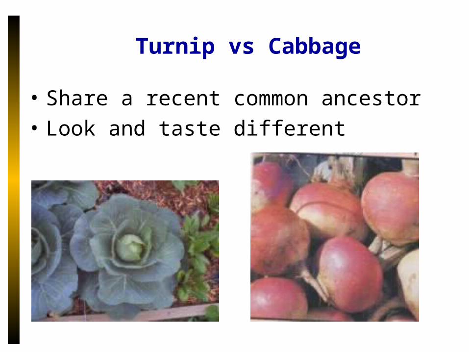
Turnip vs Cabbage
• Share a recent common ancestor
• Look and taste different
Turnip vs Cabbage
• Comparing mtDNA gene sequences yields no evolutionary information
• 99% similarity between genes
• These surprisingly identical gene sequences differed in gene order
• This study helped pave the way to analyzing genome rearrangements in molecular evolution
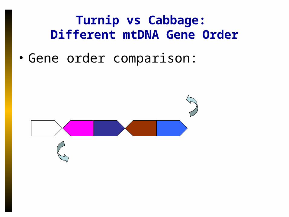
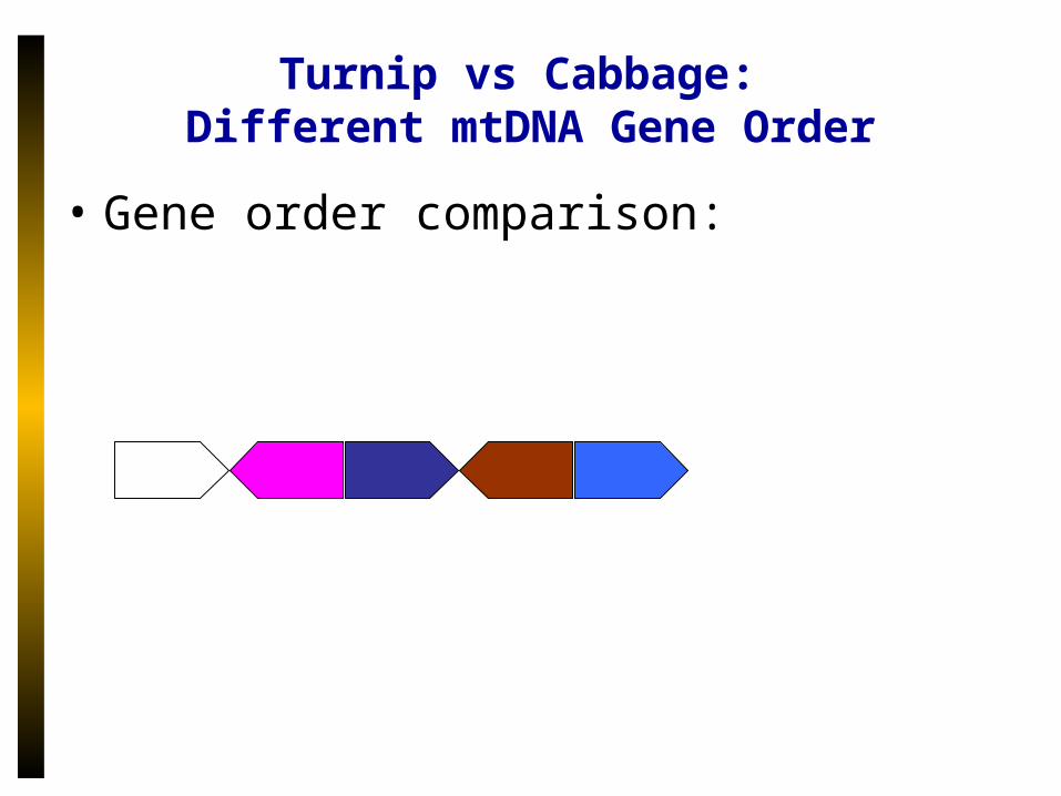
Turnip vs Cabbage: Different mtDNA Gene Order
• Gene order comparison:
Turnip vs Cabbage: Different mtDNA Gene Order
• Gene order comparison:
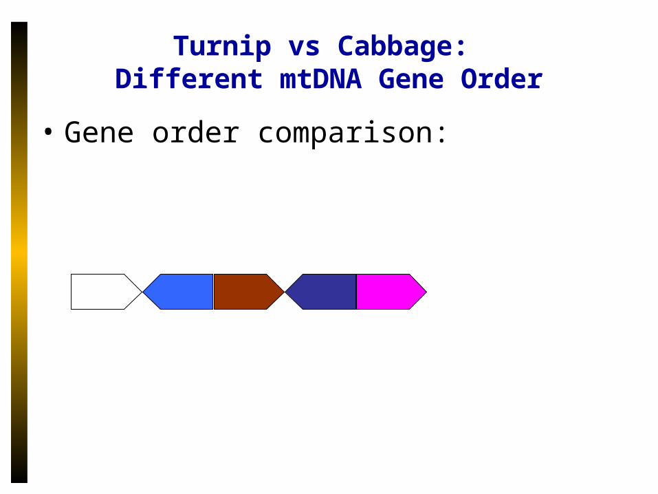
Turnip vs Cabbage: Different mtDNA Gene Order
• Gene order comparison:
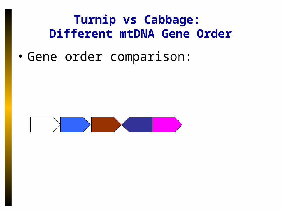
Turnip vs Cabbage: Different mtDNA Gene Order
• Gene order comparison:
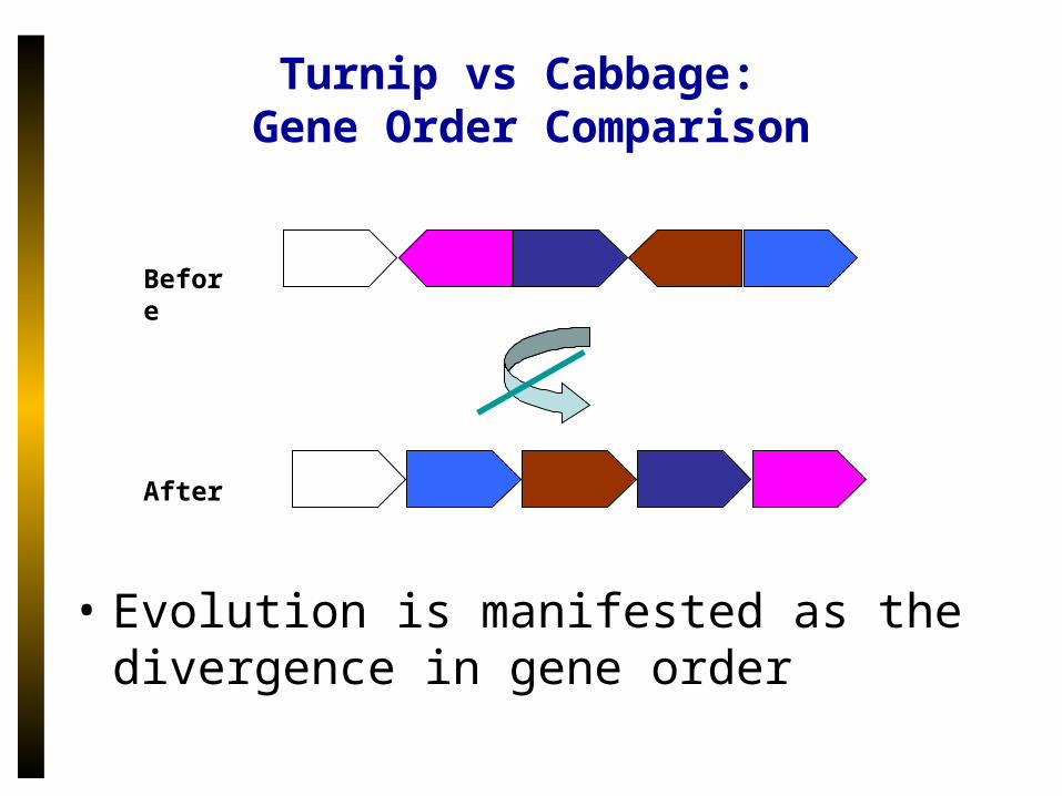
Turnip vs Cabbage: Gene Order Comparison
Before
After
• Evolution is manifested as the divergence in gene order
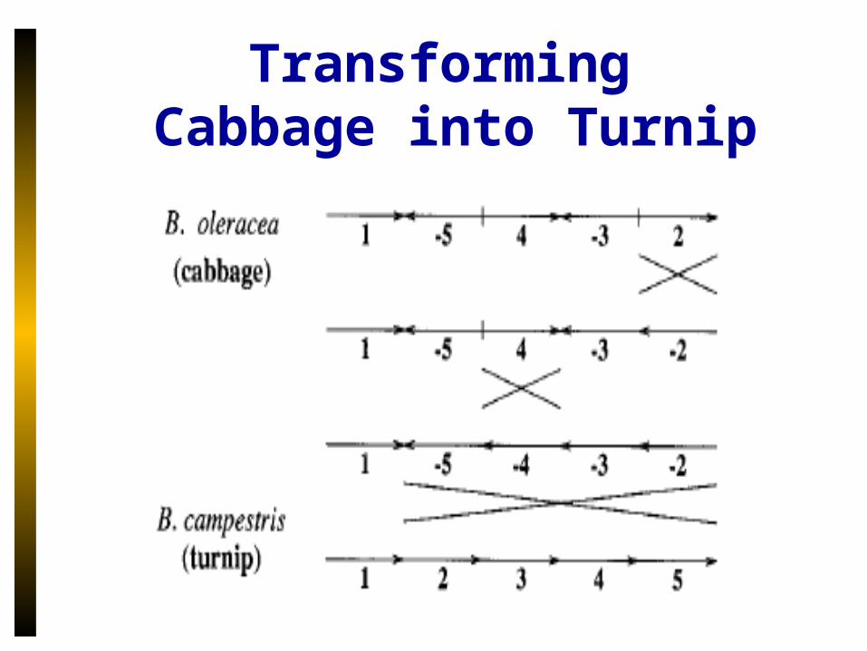
Transforming Cabbage into Turnip
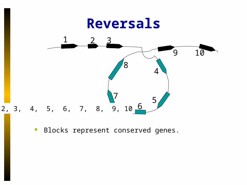
Reversals1 32
4
10
56
8
9
7
1, 2, 3, -8, -7, -6, -5, -4, 9, 10
Blocks represent conserved genes. In the course of evolution or in a clinical context, blocks
1,…,10 could be misread as 1, 2, 3, -8, -7, -6, -5, -4, 9, 10.
1, 2, 3, 4, 5, 6, 7, 8, 9, 10
Blocks represent conserved genes.
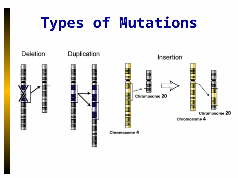
Types of Mutations
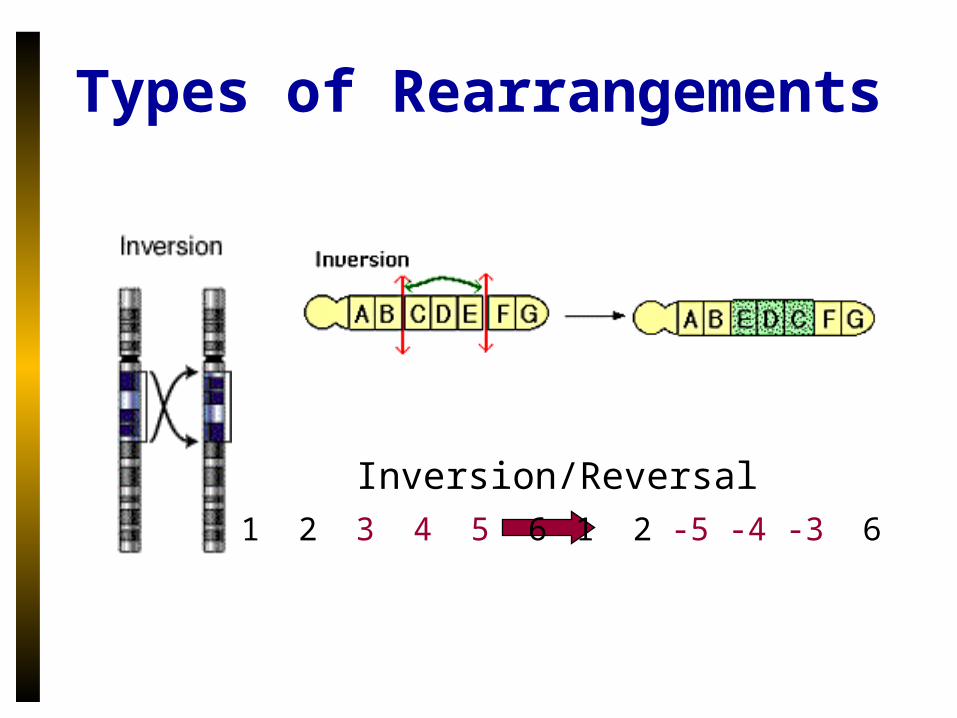
Types of Rearrangements
Inversion/Reversal1 2 3 4 5 6 1 2 -5 -4 -3 6
Types of Rearrangements
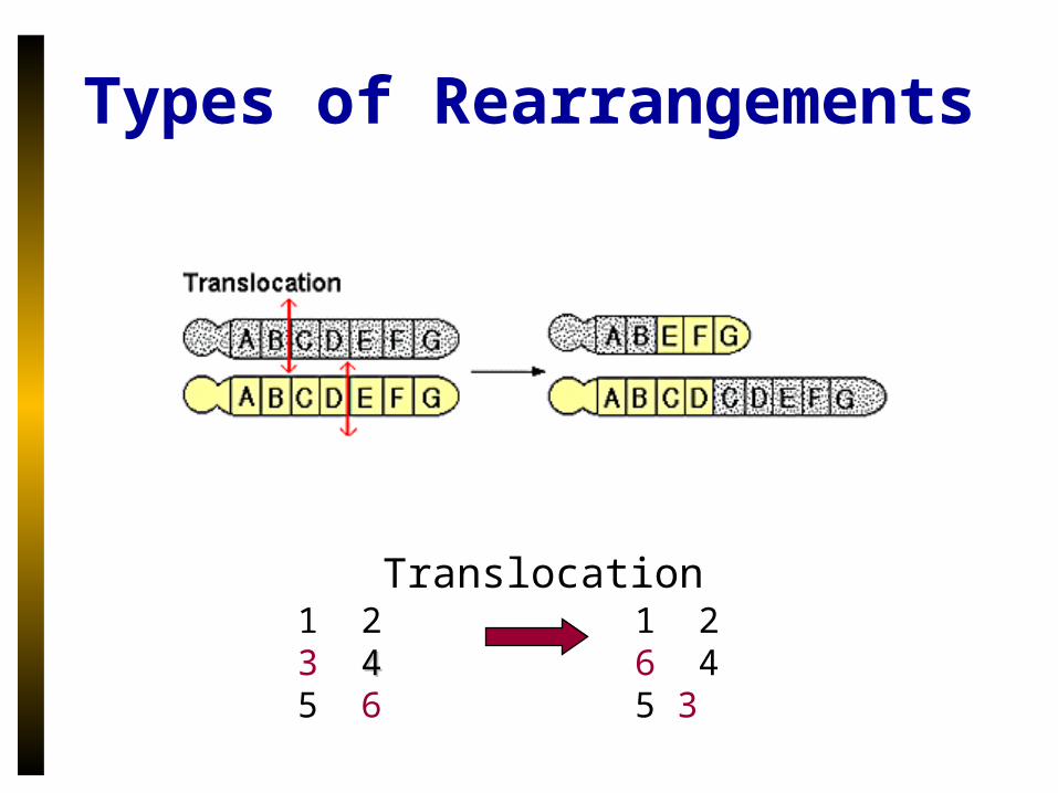
Translocation1 2 3 44 5 6
1 2 6 4 5 3
Types of Rearrangements
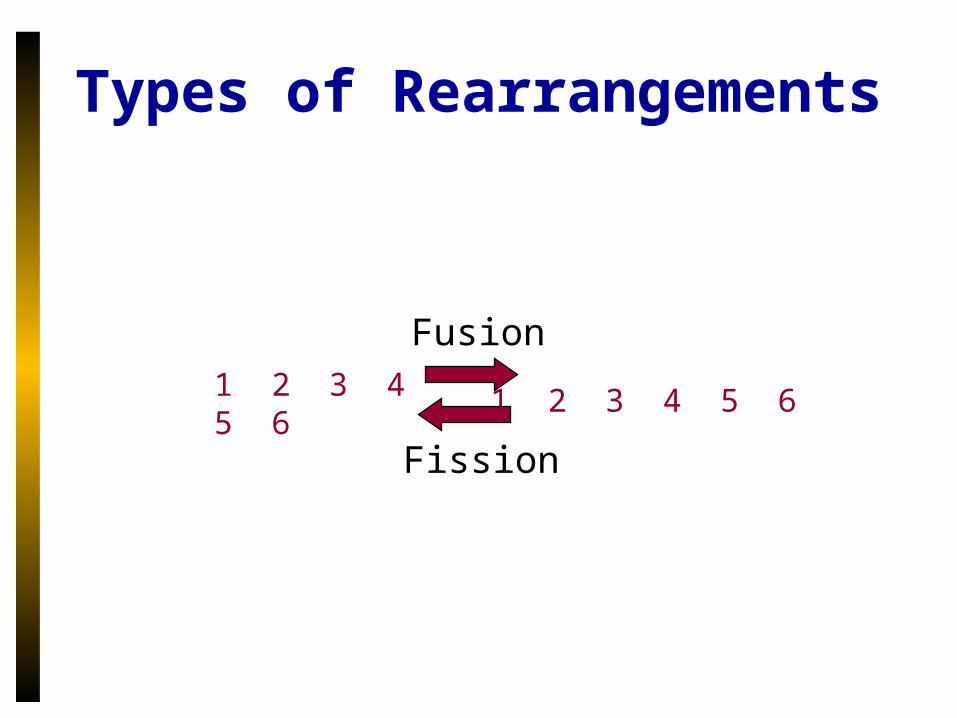
1 2 3 4 5 6
1 2 3 4 5 6
Fusion
Fission
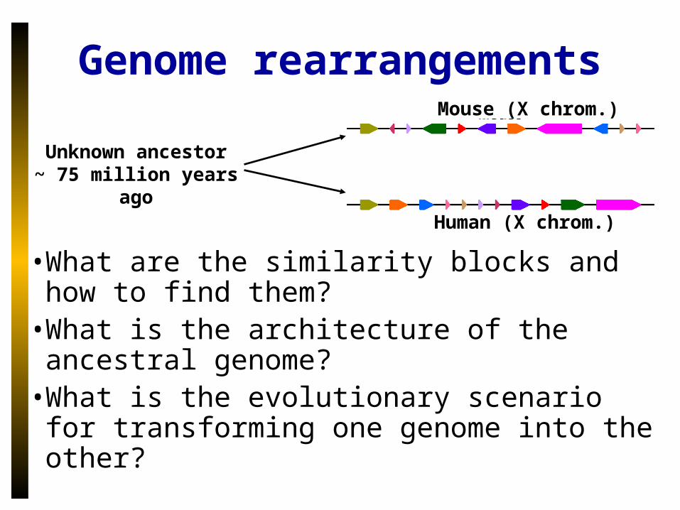
• What are the similarity blocks and how to find them?
• What is the architecture of the ancestral genome?
• What is the evolutionary scenario for transforming one genome into the other?
Unknown ancestor~ 75 million years ago
Mouse (X chrom.)
Human (X chrom.)
Genome rearrangements

Why do we care?
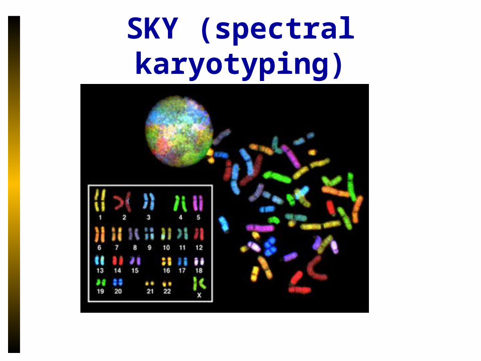
SKY (spectral karyotyping)
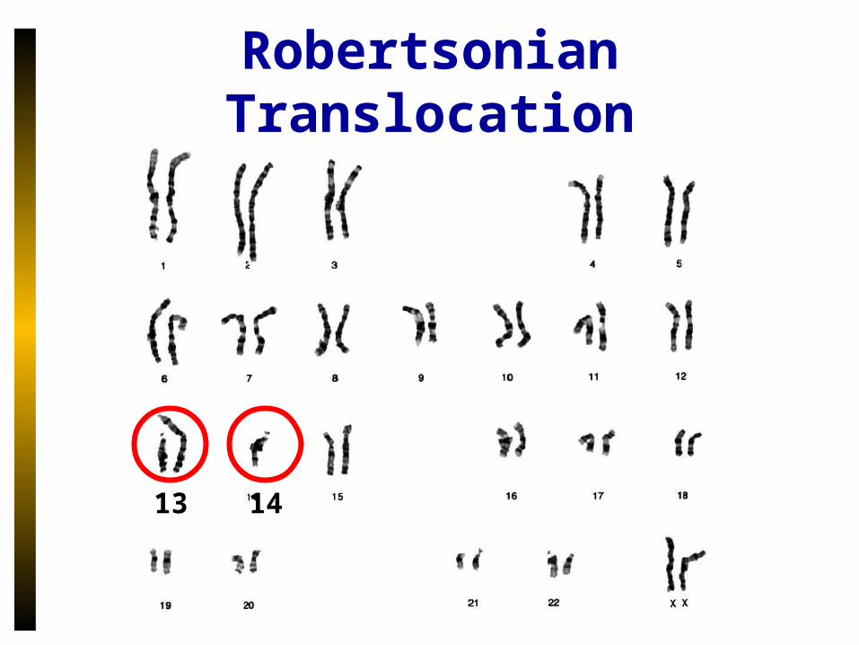
Robertsonian Translocation
13 14
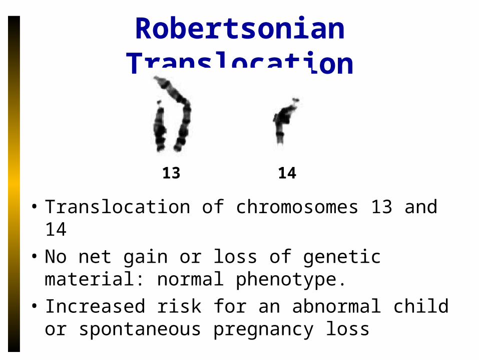
Robertsonian Translocation
• Translocation of chromosomes 13 and 14
• No net gain or loss of genetic material: normal phenotype.
• Increased risk for an abnormal child or spontaneous pregnancy loss
13 14
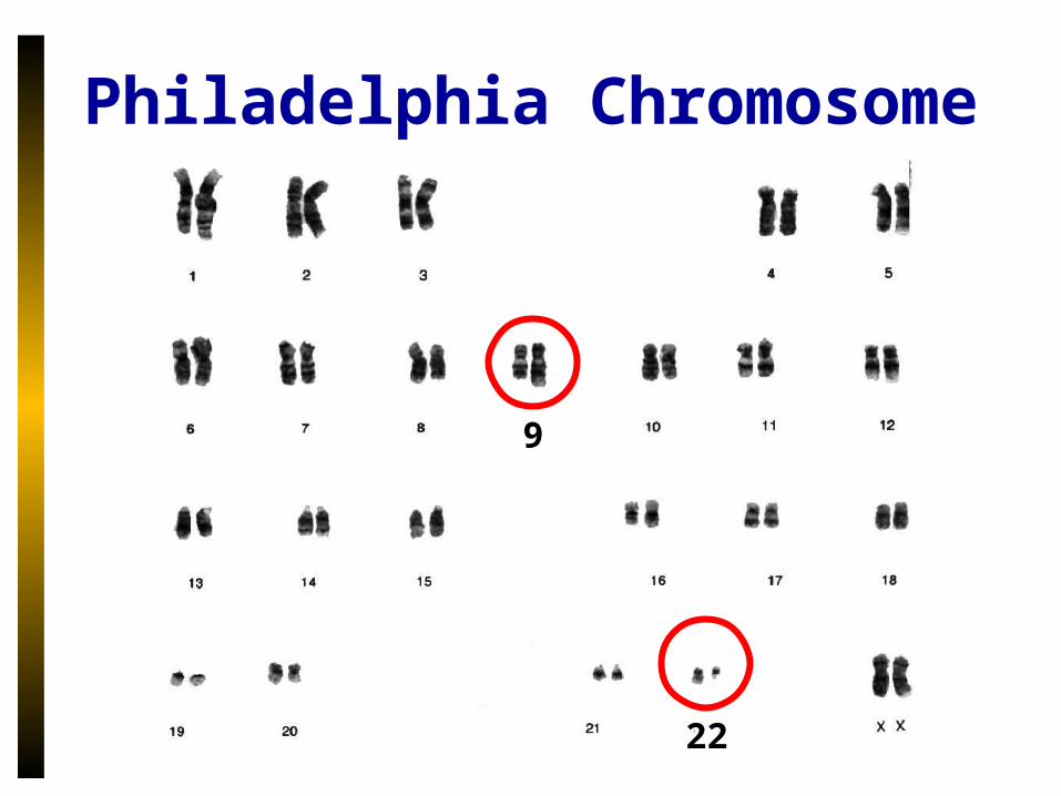
Philadelphia Chromosome
9
22
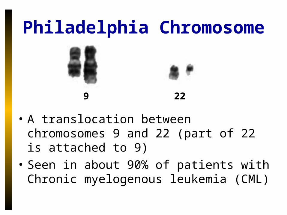
Philadelphia Chromosome
• A translocation between chromosomes 9 and 22 (part of 22 is attached to 9)
• Seen in about 90% of patients with Chronic myelogenous leukemia (CML)
9 22
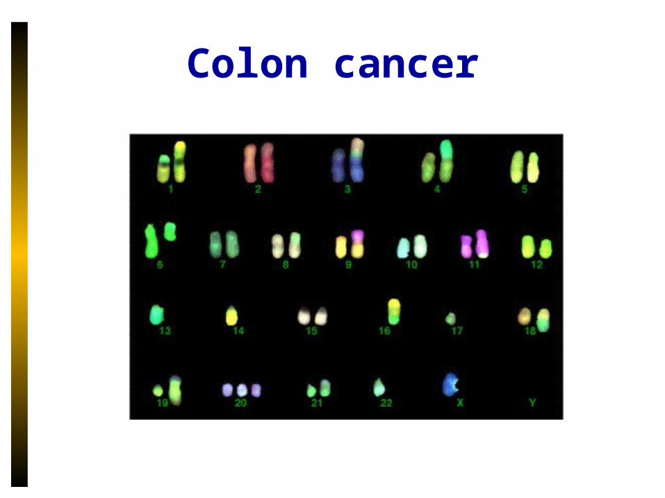
Colon cancer
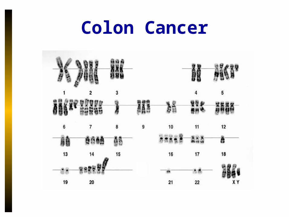
Colon Cancer

Comparative maps
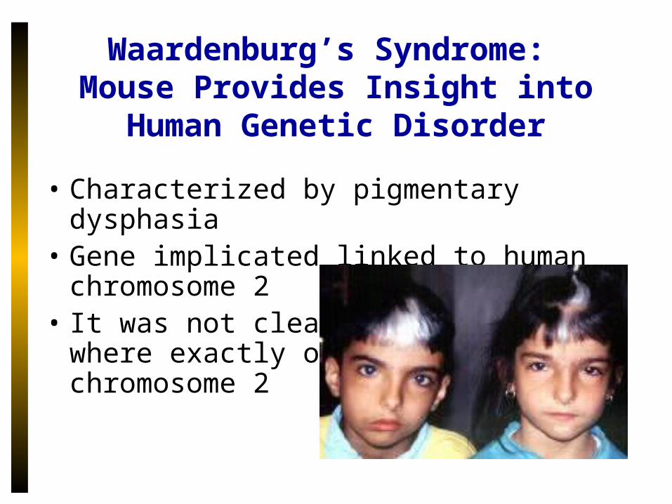
Waardenburg’s Syndrome: Mouse Provides Insight into Human
Genetic Disorder
• Characterized by pigmentary dysphasia• Gene implicated linked to human
chromosome 2 • It was not clear
where exactly on chromosome 2
Waardenburg’s syndrome and splotch mice
• A breed of mice (with splotch gene) had similar symptoms caused by the same type of gene as in humans
• Scientists identified location of gene responsible for disorder in mice
• Finding the gene in mice gives clues to where same gene is located in humans
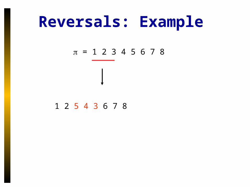
Reversals: Example
= 1 2 3 4 5 6 7 8
1 2 5 4 3 6 7 8
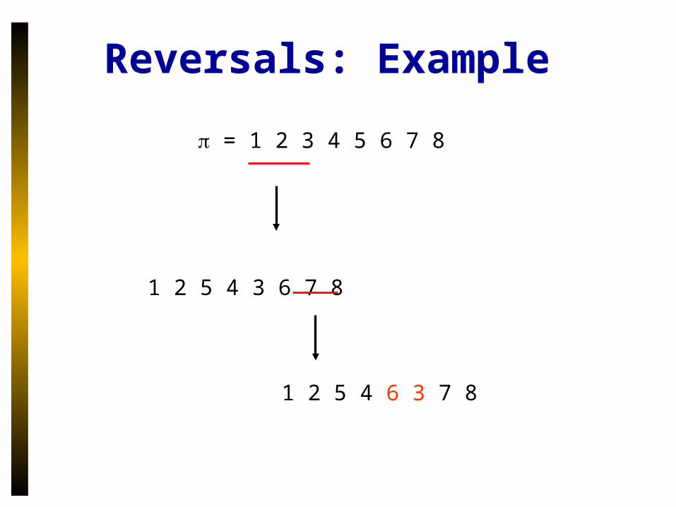
Reversals: Example
= 1 2 3 4 5 6 7 8
1 2 5 4 3 6 7 8
1 2 5 4 6 3 7 8
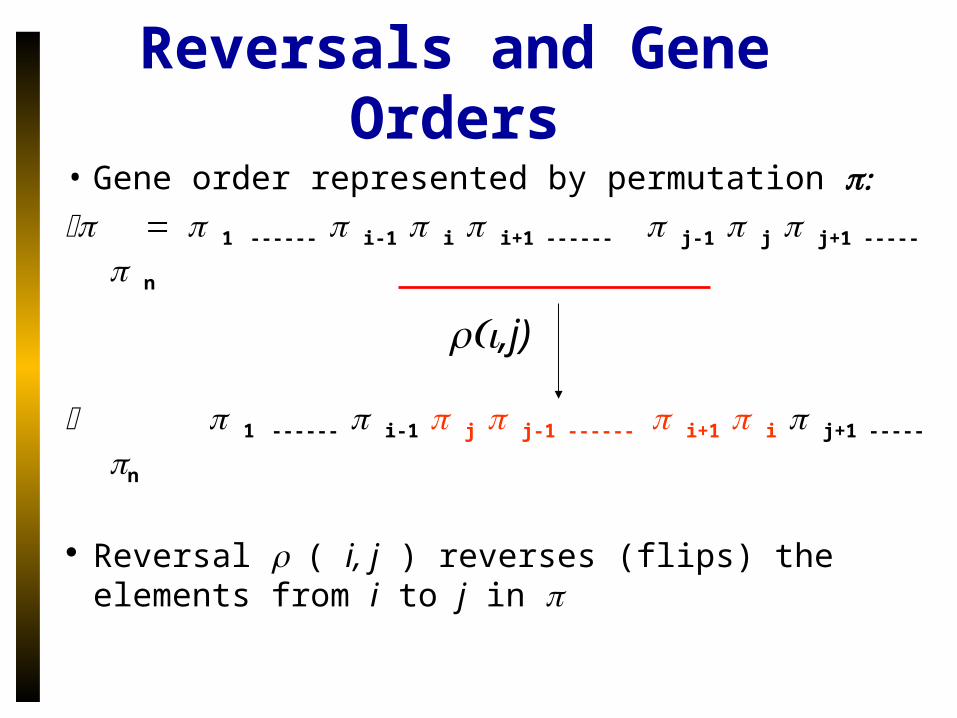
Reversals and Gene Orders
• Gene order represented by permutation 1------ i-1 i i+1 ------j-1 j j+1 -----n
1------ i-1 j j-1 ------i+1 i j+1 -----n
Reversal ( i, j ) reverses (flips) the elements from i to j in
,j)
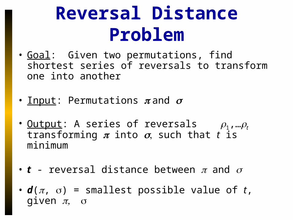
Reversal Distance Problem
• Goal: Given two permutations, find shortest series of reversals to transform one into another
• Input: Permutations and
• Output: A series of reversals 1,…t
transforming into such that t is minimum
• t - reversal distance between and
• d(, ) = smallest possible value of t, given
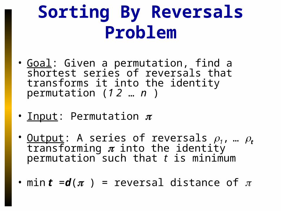
Sorting By Reversals Problem
• Goal: Given a permutation, find a shortest series of reversals that transforms it into the identity permutation (1 2 … n )
• Input: Permutation
• Output: A series of reversals 1, … t transforming into the identity permutation such that t is minimum
• min t =d( ) = reversal distance of
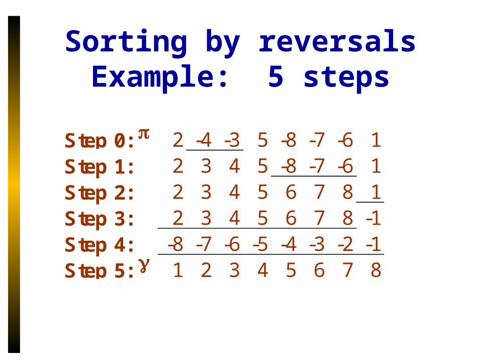
Sorting by reversalsExample: 5 steps
Step 0: 2 -4 -3 5 -8 -7 -6 1Step 1: 2 3 4 5 -8 -7 -6 1Step 2: 2 3 4 5 6 7 8 1Step 3: 2 3 4 5 6 7 8 -1Step 4: -8 -7 -6 -5 -4 -3 -2 -1Step 5: g 1 2 3 4 5 6 7 8
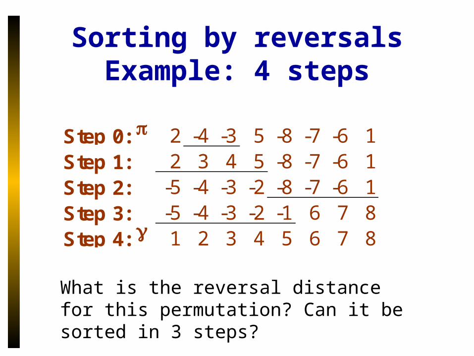
Sorting by reversalsExample: 4 steps
Step 0: 2 -4 -3 5 -8 -7 -6 1Step 1: 2 3 4 5 -8 -7 -6 1Step 2: -5 -4 -3 -2 -8 -7 -6 1Step 3: -5 -4 -3 -2 -1 6 7 8Step 4: g 1 2 3 4 5 6 7 8
What is the reversal distance for this permutation? Can it be sorted in 3 steps?

Pancake Flipping Problem• Chef prepares unordered
stack of pancakes of different sizes
• The waiter wants to sort (rearrange) them, smallest on top, largest at bottom
• He does it by flipping over several from the top, repeating this as many times as necessary
Christos Papadimitrou and Bill Gates flip pancakes
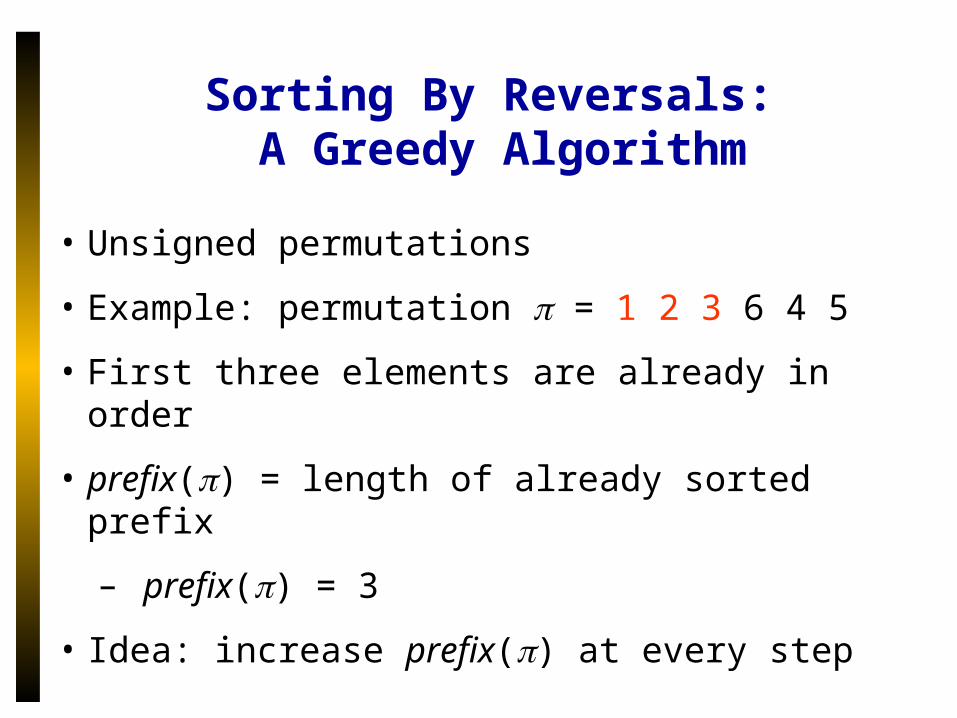
Sorting By Reversals: A Greedy Algorithm
• Unsigned permutations
• Example: permutation = 1 2 3 6 4 5
• First three elements are already in order
• prefix() = length of already sorted prefix
– prefix() = 3
• Idea: increase prefix() at every step
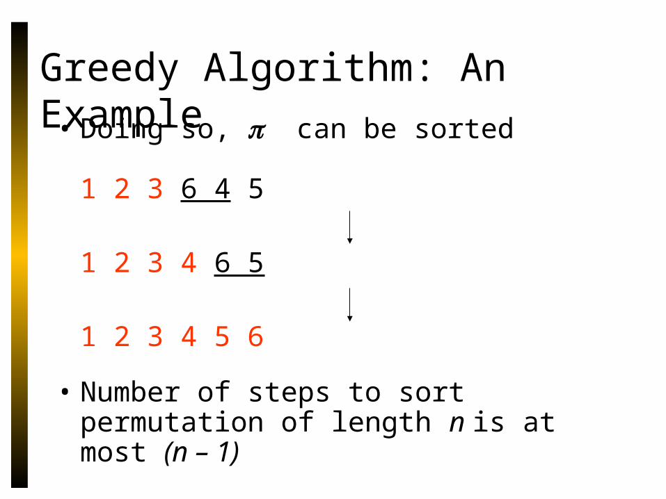
• Doing so, can be sorted
1 2 3 6 4 5
1 2 3 4 6 5
1 2 3 4 5 6
• Number of steps to sort permutation of length n is at most (n – 1)
Greedy Algorithm: An Example
Greedy Algorithm: Pseudocode
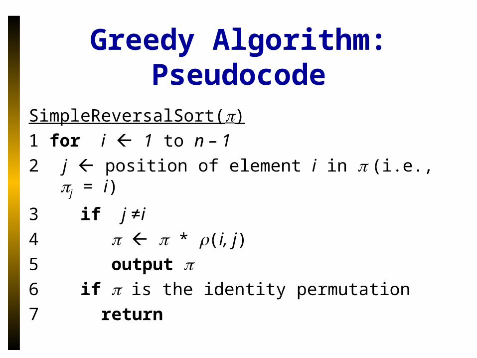
SimpleReversalSort()1 for i 1 to n – 12 j position of element i in (i.e., j = i)
3 if j ≠i4 * (i, j)5 output 6 if is the identity permutation 7 return
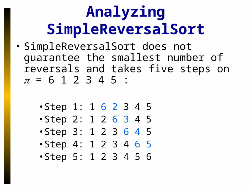
Analyzing SimpleReversalSort
• SimpleReversalSort does not guarantee the smallest number of reversals and takes five steps on = 6 1 2 3 4 5 :
•Step 1: 1 6 2 3 4 5•Step 2: 1 2 6 3 4 5 •Step 3: 1 2 3 6 4 5•Step 4: 1 2 3 4 6 5•Step 5: 1 2 3 4 5 6
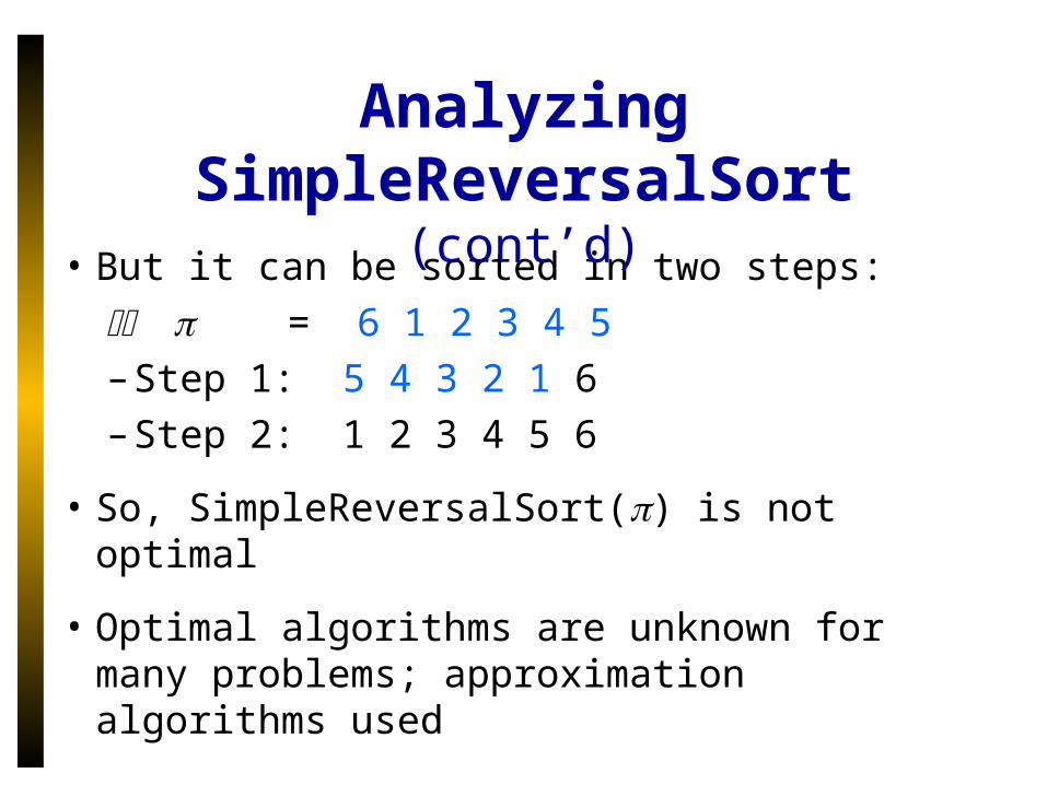
• But it can be sorted in two steps:
= 6 1 2 3 4 5 – Step 1: 5 4 3 2 1 6 – Step 2: 1 2 3 4 5 6
• So, SimpleReversalSort() is not optimal
• Optimal algorithms are unknown for many problems; approximation algorithms used
Analyzing SimpleReversalSort (cont’d)
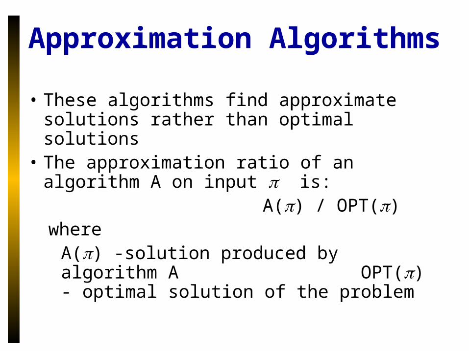
Approximation Algorithms
• These algorithms find approximate solutions rather than optimal solutions
• The approximation ratio of an algorithm A on input is: A() / OPT()where
A() -solution produced by algorithm A OPT() - optimal solution of the problem
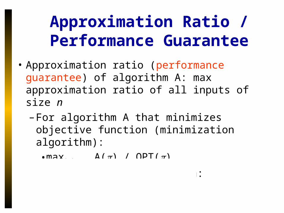
Approximation Ratio / Performance Guarantee
• Approximation ratio (performance guarantee) of algorithm A: max approximation ratio of all inputs of size n
– For algorithm A that minimizes objective function (minimization algorithm):
•max|| = n A() / OPT()
– For maximization algorithm:
•min|| = n A() / OPT()
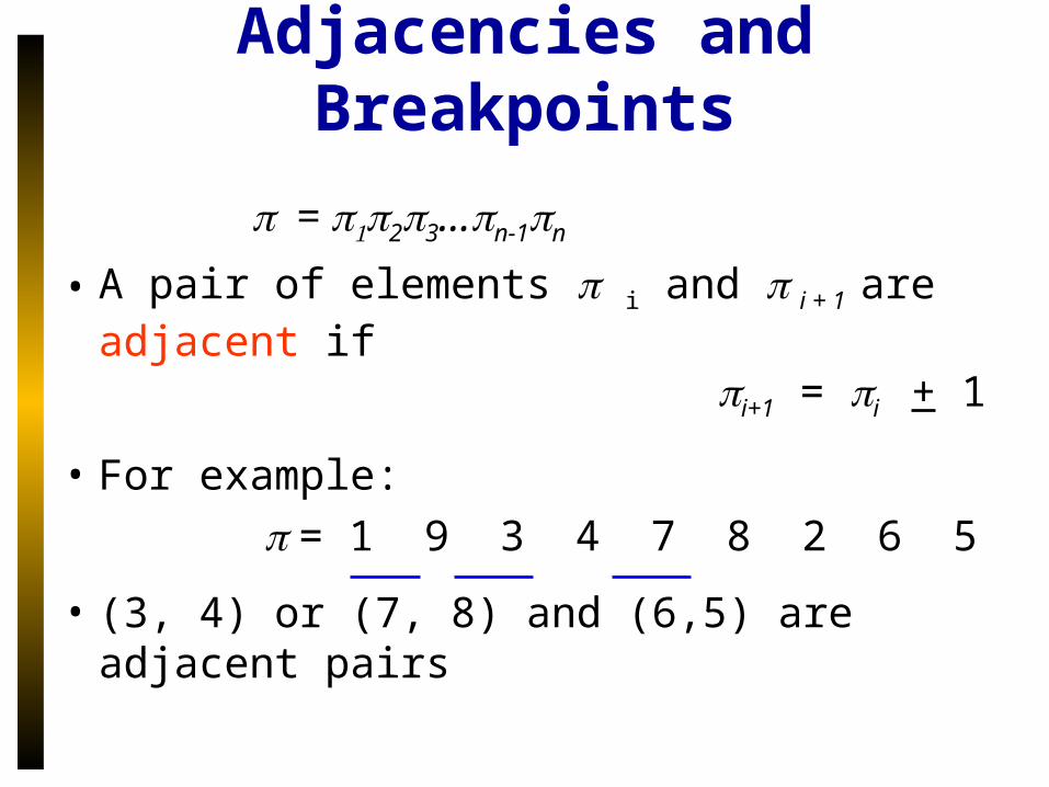
= 23…n-1n
• A pair of elements i and i + 1 are adjacent if
i+1 = i + 1
• For example:
= 1 9 3 4 7 8 2 6 5
• (3, 4) or (7, 8) and (6,5) are adjacent pairs
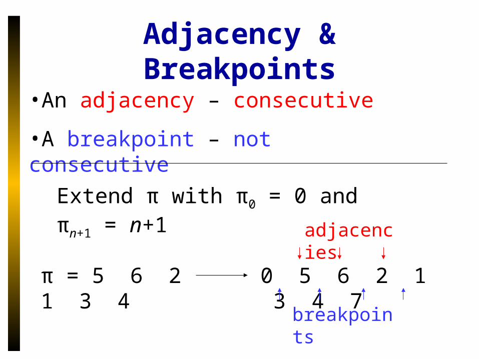
Adjacencies and Breakpoints
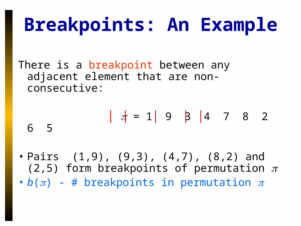
There is a breakpoint between any adjacent element that are non-consecutive:
= 1 9 3 4 7 8 2 6 5
• Pairs (1,9), (9,3), (4,7), (8,2) and (2,5) form breakpoints of permutation
• b() - # breakpoints in permutation
Breakpoints: An Example
Adjacency & Breakpoints
•An adjacency – consecutive
•A breakpoint – not consecutive
π = 5 6 2 1 3 4 0 5 6 2 1 3 4 7
adjacencies
breakpoints
Extend π with π0 = 0 and πn+1 = n+1
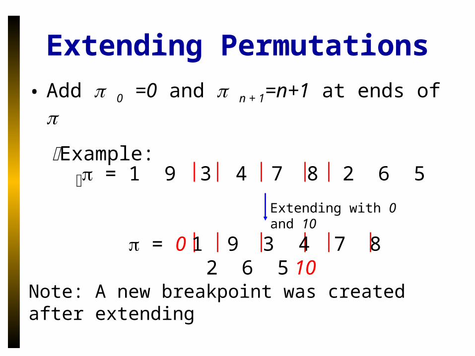
• Add 0 =0 and n + 1=n+1 at ends of
Example:
Extending with 0 and 10
Note: A new breakpoint was created after extending
Extending Permutations
= 1 9 3 4 7 8 2 6 5
= 0 1 9 3 4 7 8 2 6 5 10
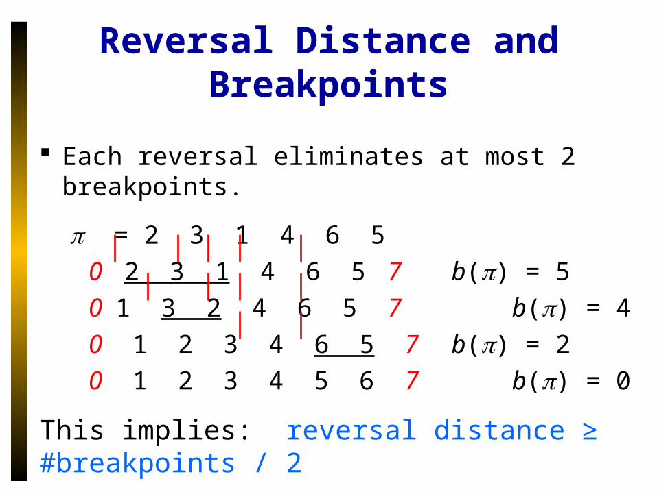
Each reversal eliminates at most 2 breakpoints.
= 2 3 1 4 6 5
0 2 3 1 4 6 5 7 b() = 5
0 1 3 2 4 6 5 7 b() = 4
0 1 2 3 4 6 5 7 b() = 2
0 1 2 3 4 5 6 7 b() = 0
Reversal Distance and Breakpoints
This implies: reversal distance ≥ #breakpoints / 2
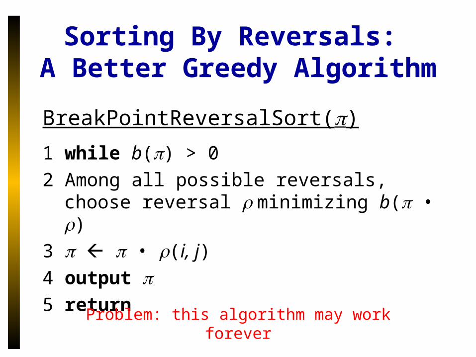
Sorting By Reversals: A Better Greedy Algorithm
BreakPointReversalSort()
1 while b() > 02 Among all possible reversals,
choose reversal minimizing b( • )3 • (i, j)4 output 5 return
Problem: this algorithm may work forever
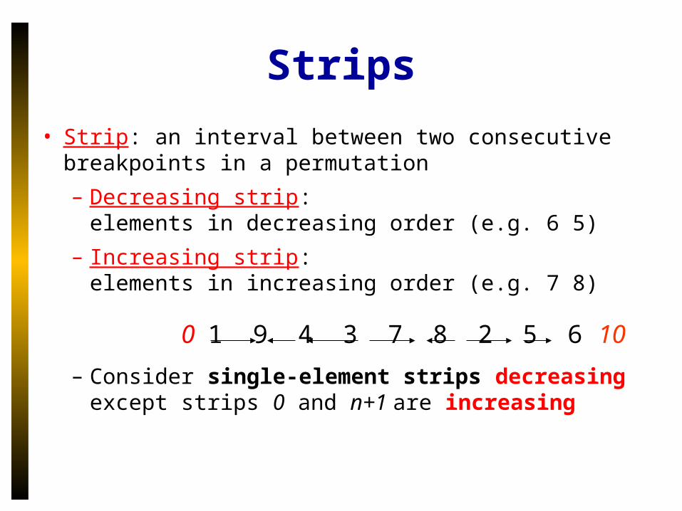
Strips
• Strip: an interval between two consecutive breakpoints in a permutation
– Decreasing strip: elements in decreasing order (e.g. 6 5)
– Increasing strip: elements in increasing order (e.g. 7 8)
0 1 9 4 3 7 8 2 5 6 10
– Consider single-element strips decreasing except strips 0 and n+1 are increasing
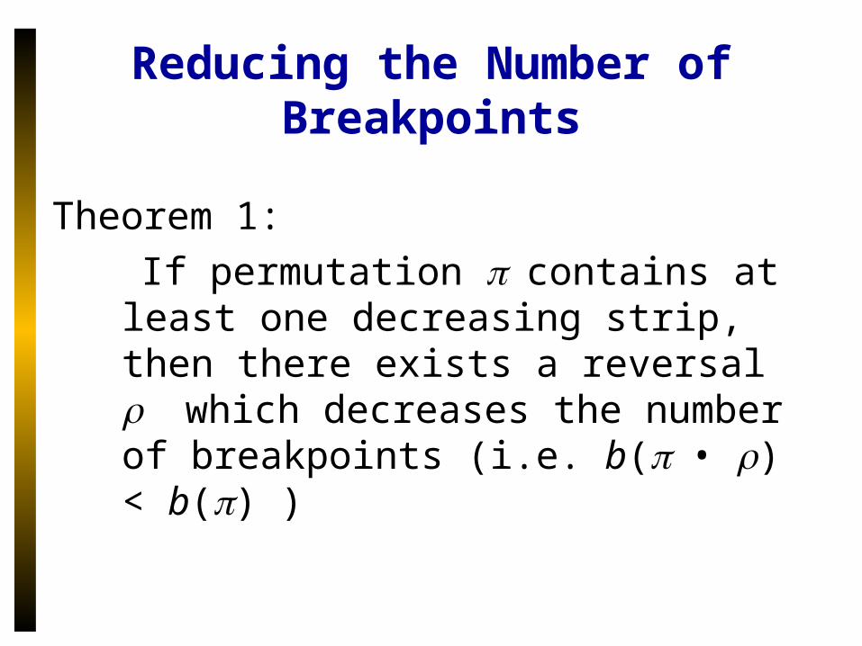
Reducing the Number of Breakpoints
Theorem 1:
If permutation contains at least one decreasing strip, then there exists a reversal which decreases the number of breakpoints (i.e. b(• ) < b() )
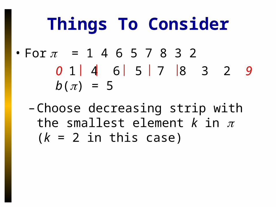
Things To Consider
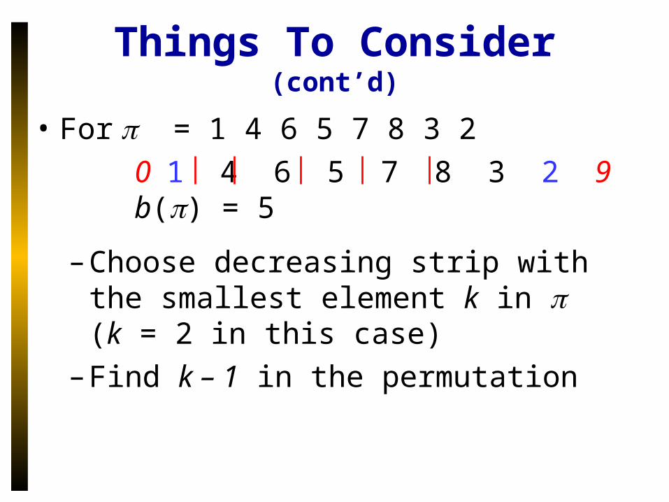
• For = 1 4 6 5 7 8 3 2
0 1 4 6 5 7 8 3 2 9 b() = 5
– Choose decreasing strip with the smallest element k in (k = 2 in this case)
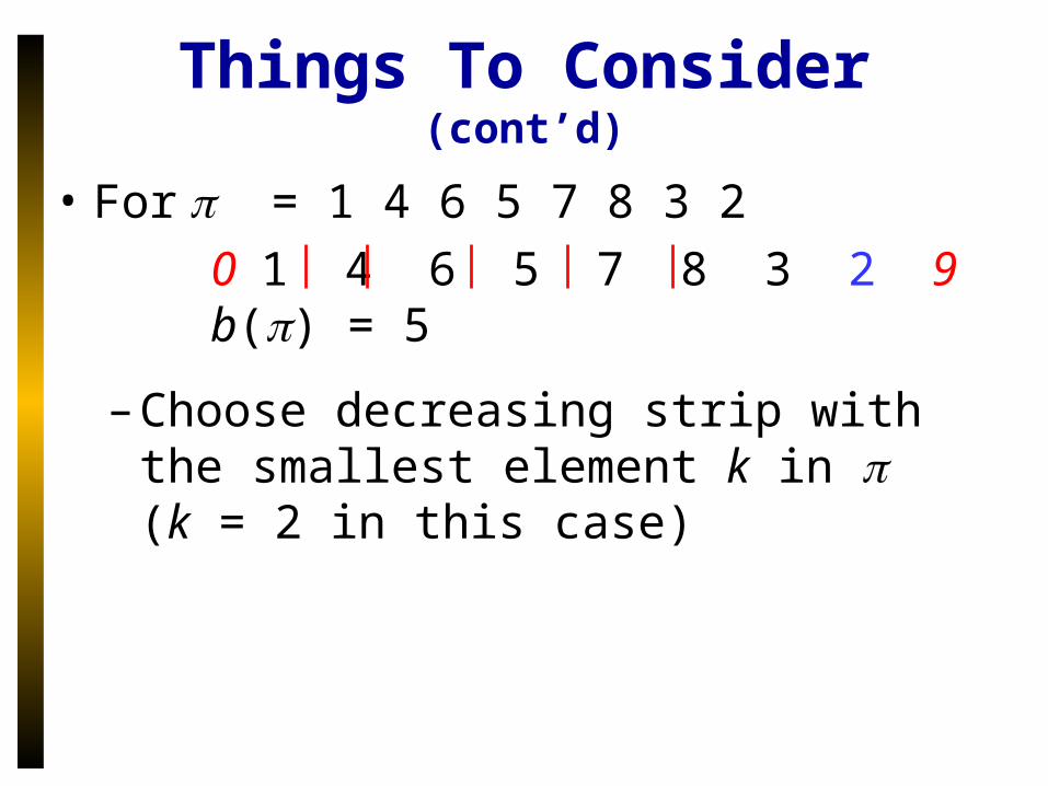
Things To Consider (cont’d)
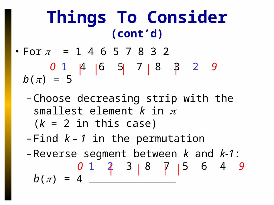
• For = 1 4 6 5 7 8 3 2
0 1 4 6 5 7 8 3 2 9 b() = 5
– Choose decreasing strip with the smallest element k in (k = 2 in this case)
Things To Consider (cont’d)
• For = 1 4 6 5 7 8 3 2
0 1 4 6 5 7 8 3 2 9 b() = 5
– Choose decreasing strip with the smallest element k in (k = 2 in this case)
– Find k – 1 in the permutation
Things To Consider (cont’d)
• For = 1 4 6 5 7 8 3 2
0 1 4 6 5 7 8 3 2 9 b() = 5
– Choose decreasing strip with the smallest element k in (k = 2 in this case)
– Find k – 1 in the permutation
– Reverse segment between k and k-1: 0 1 2 3 8 7 5 6 4 9 b() = 4
Reducing the Number of Breakpoints Again
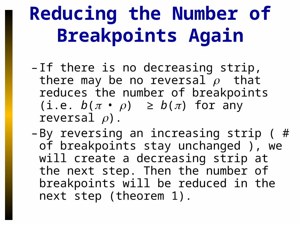
– If there is no decreasing strip, there may be no reversal that reduces the number of breakpoints (i.e. b(•) ≥ b() for any reversal ).
– By reversing an increasing strip ( # of breakpoints stay unchanged ), we will create a decreasing strip at the next step. Then the number of breakpoints will be reduced in the next step (theorem 1).
Things To Consider (cont’d)
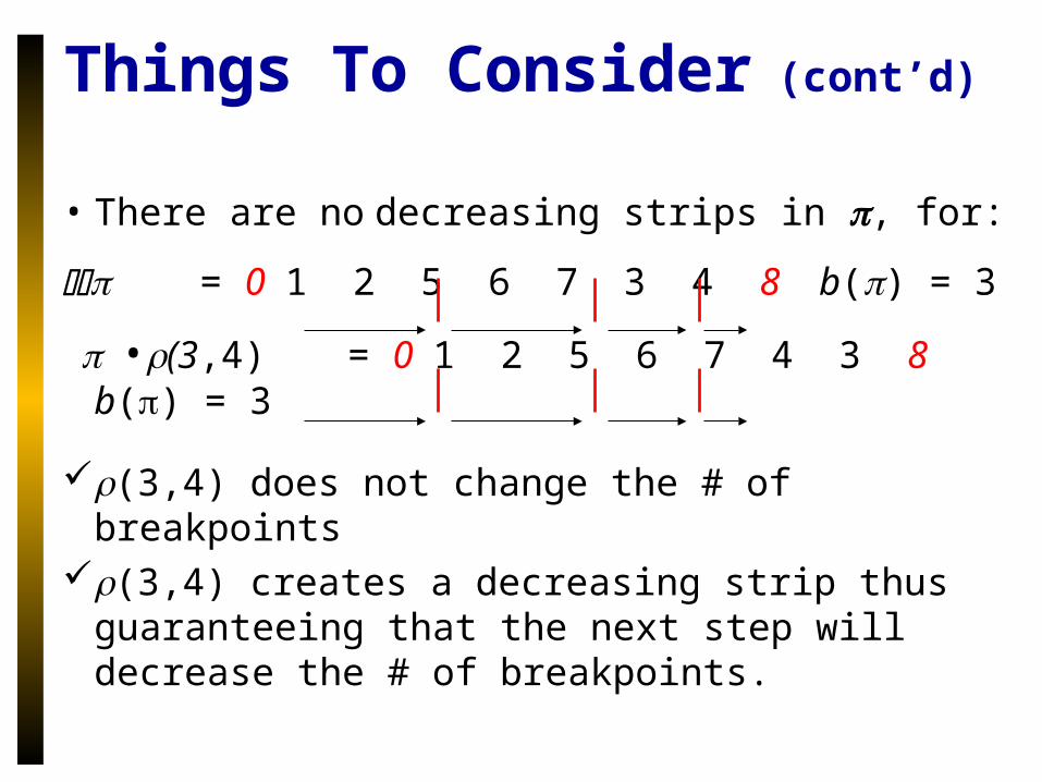
• There are no decreasing strips in , for:
= 0 1 2 5 6 7 3 4 8 b() = 3
•(3,4) = 0 1 2 5 6 7 4 3 8 b() = 3
(3,4) does not change the # of breakpoints(3,4) creates a decreasing strip thus
guaranteeing that the next step will decrease the # of breakpoints.
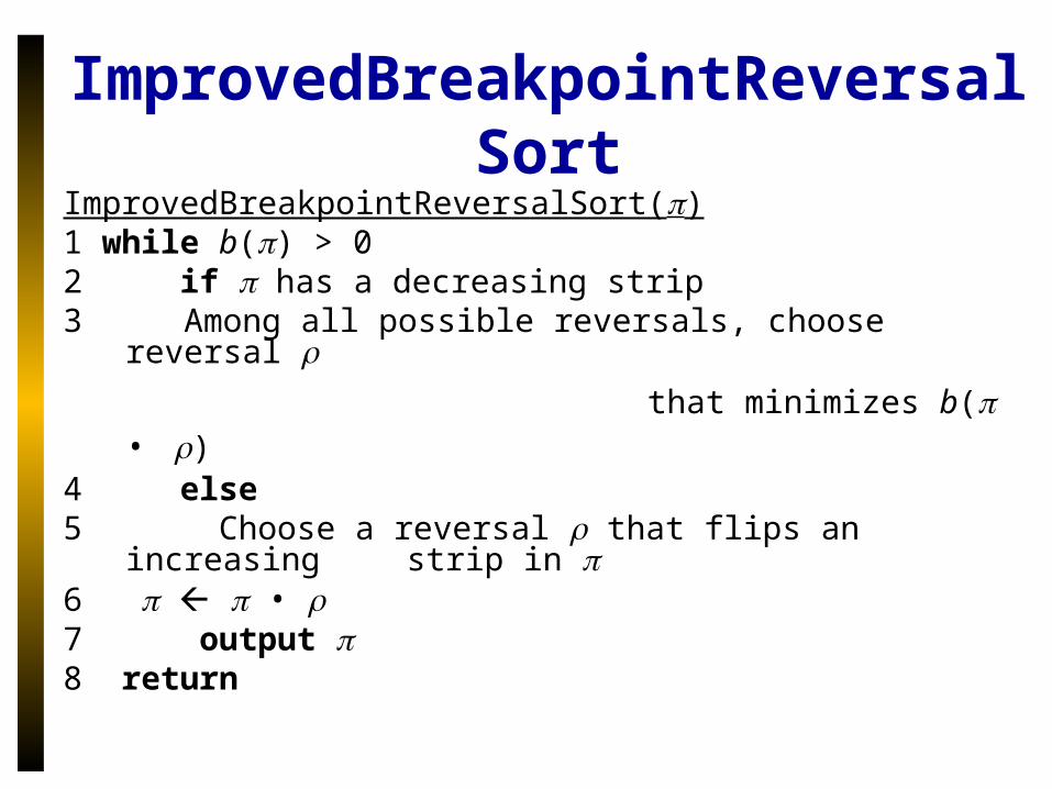
ImprovedBreakpointReversalSortImprovedBreakpointReversalSort()1 while b() > 02 if has a decreasing strip3 Among all possible reversals, choose reversal
that minimizes b( • )4 else5 Choose a reversal that flips an increasing
strip in 6 • 7 output 8 return
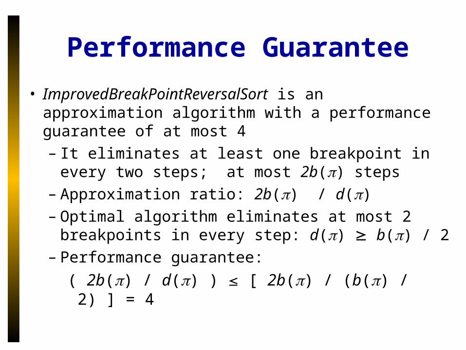
• ImprovedBreakPointReversalSort is an approximation algorithm with a performance guarantee of at most 4– It eliminates at least one breakpoint in every
two steps; at most 2b() steps– Approximation ratio: 2b() / d()– Optimal algorithm eliminates at most 2
breakpoints in every step: d() b() / 2– Performance guarantee:
( 2b() / d() ) [ 2b() / (b() / 2) ] = 4
Performance Guarantee
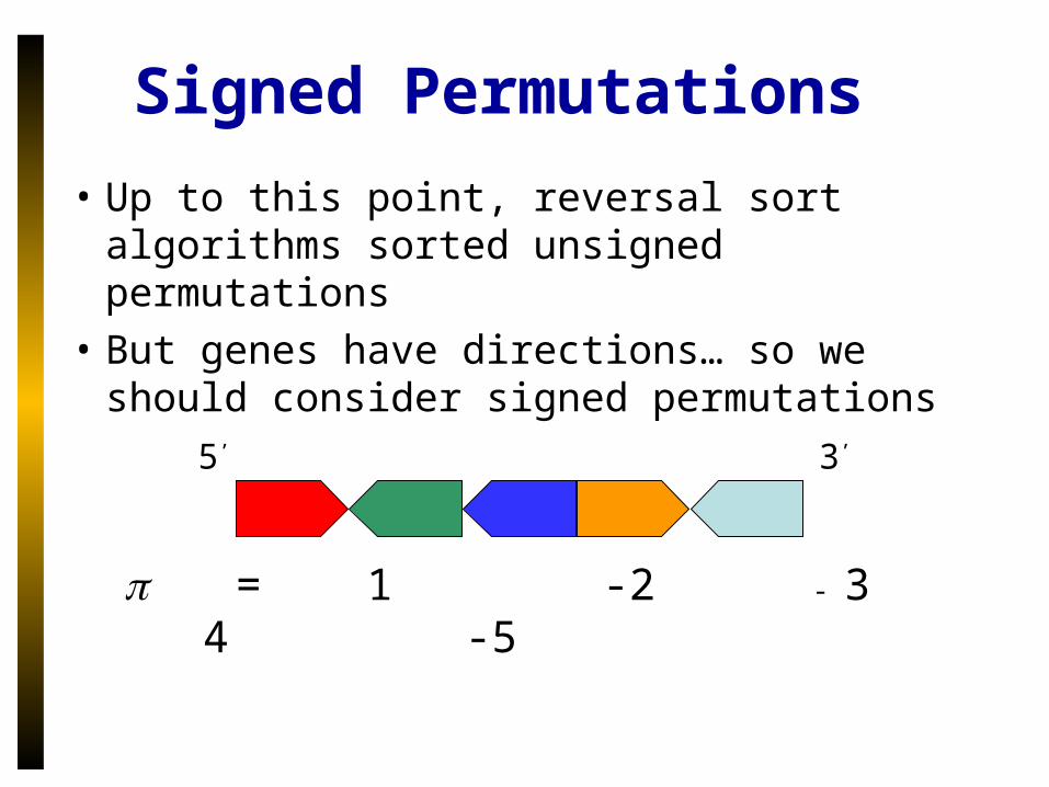
Signed Permutations
• Up to this point, reversal sort algorithms sorted unsigned permutations
• But genes have directions… so we should consider signed permutations
5’ 3’
= 1 -2 - 3 4 -5
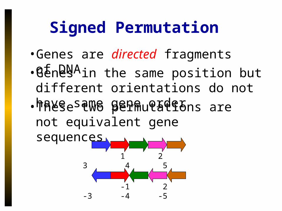
Signed Permutation
• Genes are directed fragments of DNA
• Genes in the same position but different orientations do not have same gene order
• These two permutations are not equivalent gene sequences
1 2 3 4 5
-1 2 -3 -4 -5
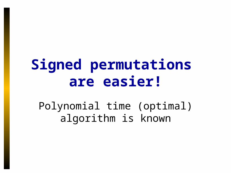
Signed permutations are easier!
Polynomial time (optimal) algorithm is known

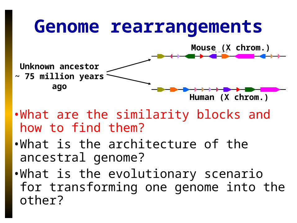
• What are the similarity blocks and how to find them?
• What is the architecture of the ancestral genome?
• What is the evolutionary scenario for transforming one genome into the other?
Unknown ancestor~ 75 million years ago
Mouse (X chrom.)
Human (X chrom.)
Genome rearrangements
• What are the similarity blocks and how to find them?
• What is the architecture of the ancestral genome?
• What is the evolutionary scenario for transforming one genome into the other?
Unknown ancestor~ 75 million years ago
Mouse (X chrom.)
Human (X chrom.)
Genome rearrangements
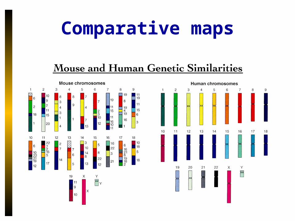
Comparative maps
A brief history
• Chromosome comparisons– no information about genes
• 1920’s: Sturtevant, Weinstein
• Today: many organisms, many uses
• Humans:– primates, mouse, cat, dog, zebrafish, ...– Alzheimer, cancers, diabetes, obesity, ...
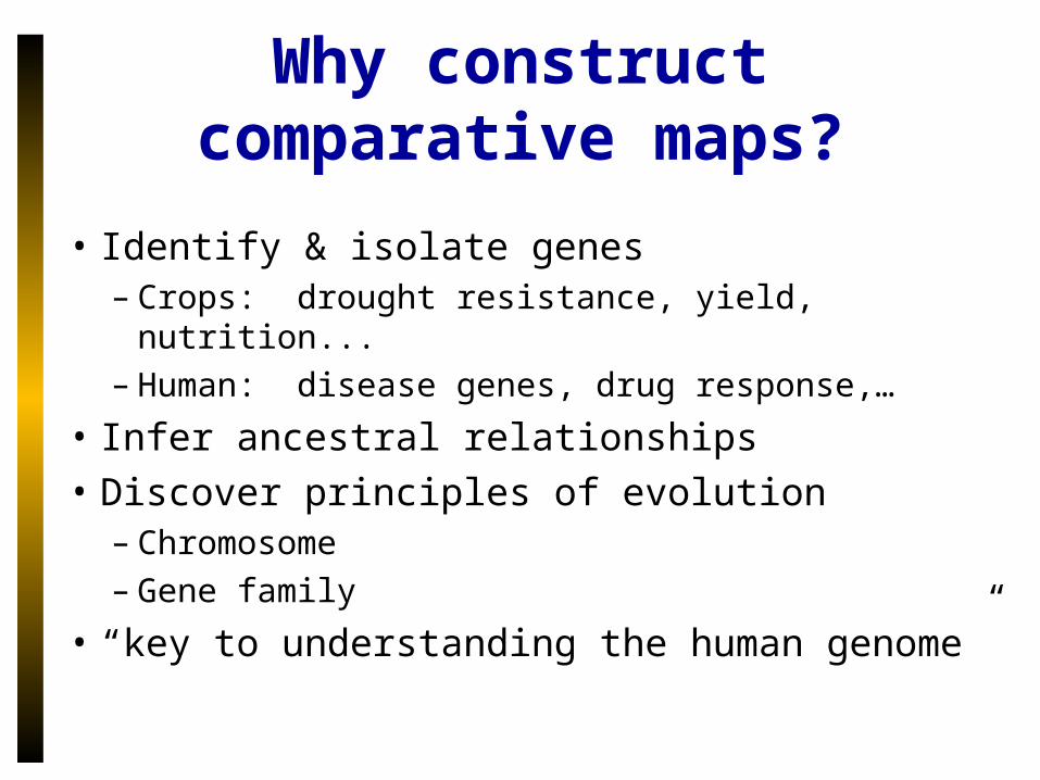
Why construct comparative maps?
• Identify & isolate genes– Crops: drought resistance, yield, nutrition...– Human: disease genes, drug response,…
• Infer ancestral relationships
• Discover principles of evolution– Chromosome– Gene family
• “key to understanding the human genome”
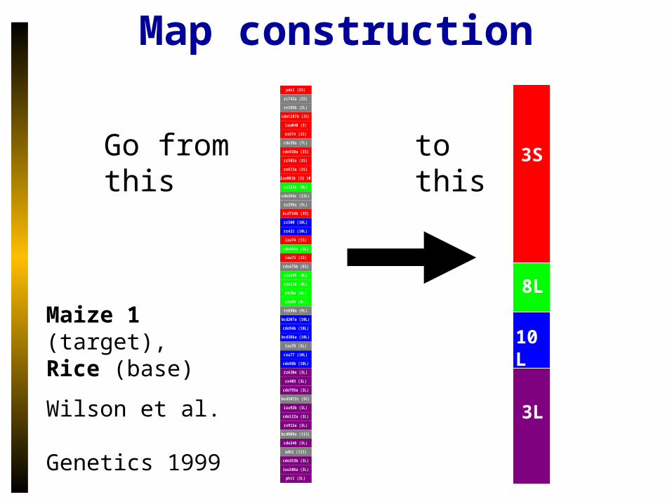
Map construction
3S
8L
10L
3L
Maize 1 (target), Rice (base)
Wilson et al. Genetics 1999
pds1 (3S)
rz742a (2S)
rz103b (2L)
cdo1387b (3S)
isu040 (3)
rz574 (3S)
cdo38a (7L)
cdo938a (3S)
rz585a (3S)
rz672a (3S)
isu081b (3S 10L)
rz323a (8L)
cdo344c (12L)
rz296a (5L)
bcd734b (3S)
rz500 (10L)
rz421 (10L)
isu74 (3S)
cdo464a (8L)
isu73 (3S)
cdo475b (6S)
cdo595 (8L)
cdo116 (8L)
rz28a (8L)
cdo99 (8L)
rz698a (9L)
bcd207a (10L)
cdo94b (10L)
bcd386a (10L)
isu78 (5L)
csu77 (10L)
cdo98b (10L)
rz630e (3L)
rz403 (3L)
cdo795a (3L)
bcd1072c (5C)
isu92b (3L)
cdo122a (3L)
rz912a (3L)
bcd808a (11S)
cdo246 (3L)
adh1 (11S)
cdo353b (3L)
isu106a (3L)
phi1 (3L)
Go from this to this

Why automate?
• Time consuming, laborious– Needs to be redone frequently
• Codify a common set of principles
• Nadeau and Sankoff: warn of “arbitrary nature of comparative map construction”
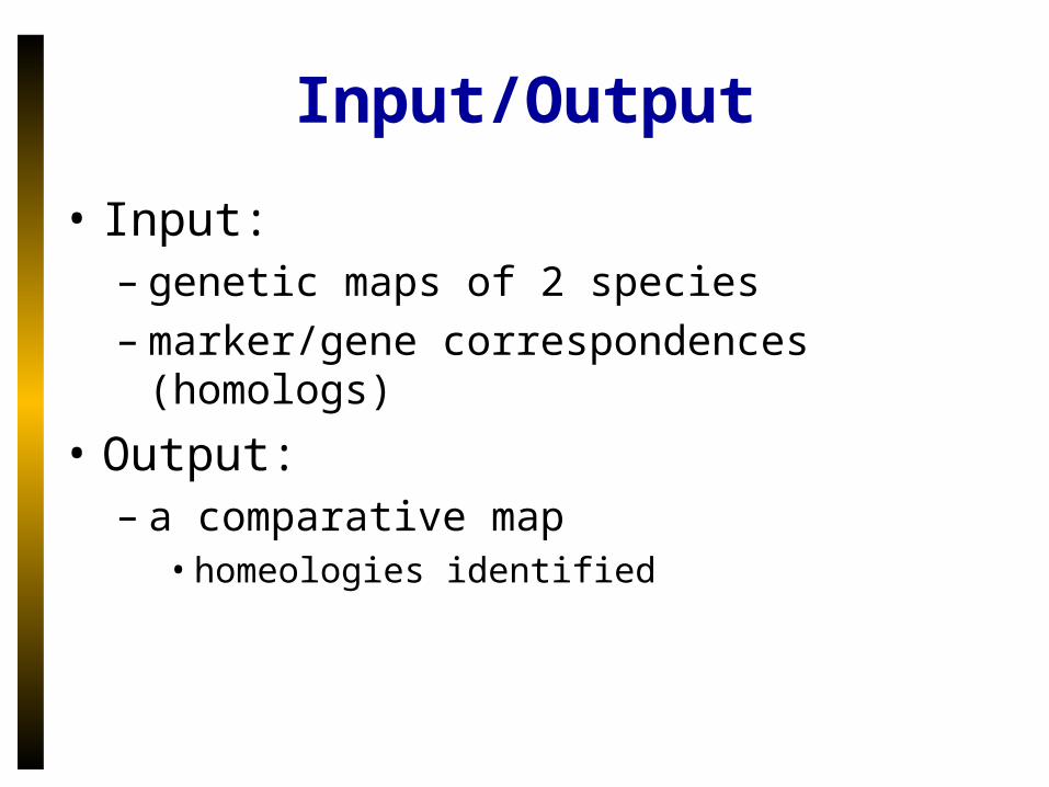
Input/Output
• Input: – genetic maps of 2 species– marker/gene correspondences (homologs)
• Output:– a comparative map
• homeologies identified
A natural model?
Maize 1 (target),
Rice (base)
Wilson et al. Genetics 1999
Maize 1
pds1 (3S)
rz742a (2S)
rz103b (2L)
cdo1387b (3S)
isu040 (3)
rz574 (3S)
cdo38a (7L)
cdo938a (3S)
rz585a (3S)
rz672a (3S)
isu081b (3S 10L)
rz323a (8L)
cdo344c (12L)
rz296a (5L)
bcd734b (3S)
rz500 (10L)
rz421 (10L)
isu74 (3S)
cdo464a (8L)
isu73 (3S)
cdo475b (6S)
cdo595 (8L)
cdo116 (8L)
rz28a (8L)
cdo99 (8L)
rz698a (9L)
bcd207a (10L)
cdo94b (10L)
bcd386a (10L)
isu78 (5L)
csu77 (10L)
cdo98b (10L)
rz630e (3L)
rz403 (3L)
cdo795a (3L)
bcd1072c (5C)
isu92b (3L)
cdo122a (3L)
rz912a (3L)
bcd808a (11S)
cdo246 (3L)
adh1 (11S)
cdo353b (3L)
isu106a (3L)
phi1 (3L)
Rice
3S
8L
10L
3L
Scoring
10L
3L
s
m
bcd207a (10L)cdo94b (10L)bcd386a (10L)isu78 (5L)csu77 (10L)cdo98b (10L)rz630e (3L)rz403 (3L)cdo795a (3L)isu92b (3L)
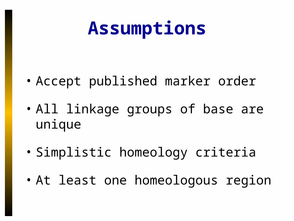
Assumptions
• Accept published marker order
• All linkage groups of base are unique
• Simplistic homeology criteria
• At least one homeologous region
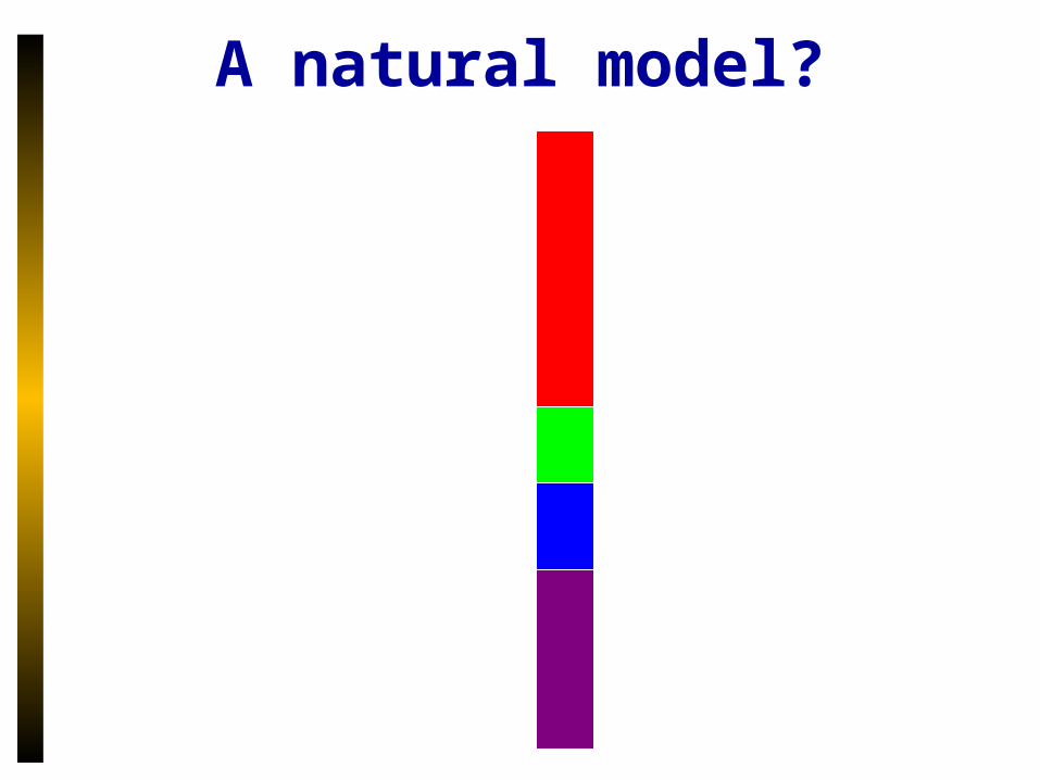
A natural model?
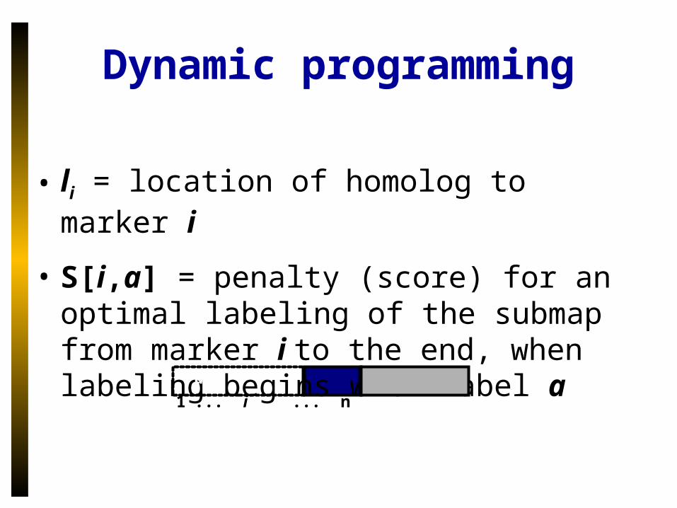
Dynamic programming
• li = location of homolog to marker i
• S[i,a] = penalty (score) for an optimal labeling of the submap from marker i to the end, when labeling begins with label a
a
1 ... i ... n
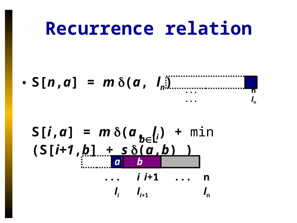
Recurrence relation
• S[n,a] = m (a, ln)
S[i,a] = m (a, li) + min (S[i+1,b] + s (a,b) )bL
a b
... i i+1 ... n
li li+1 ln
a ... n... ln
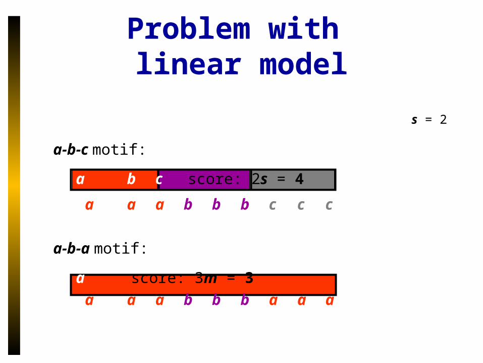
Problem with linear model
s = 2
a-b-c motif:
a b c score: 2s = 4
a a a b b b c c c
a-b-a motif:
a score: 3m = 3
a a a b b b a a a
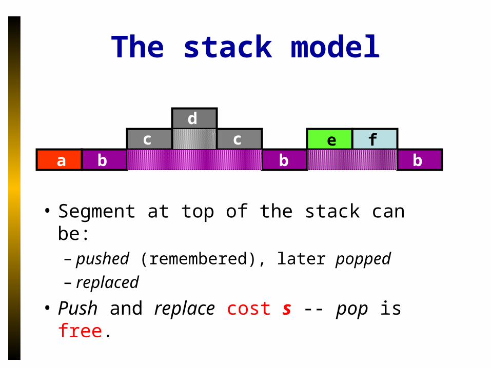
The stack model
• Segment at top of the stack can be:– pushed (remembered), later popped– replaced
• Push and replace cost s -- pop is free.
b b bfe
dc
ac
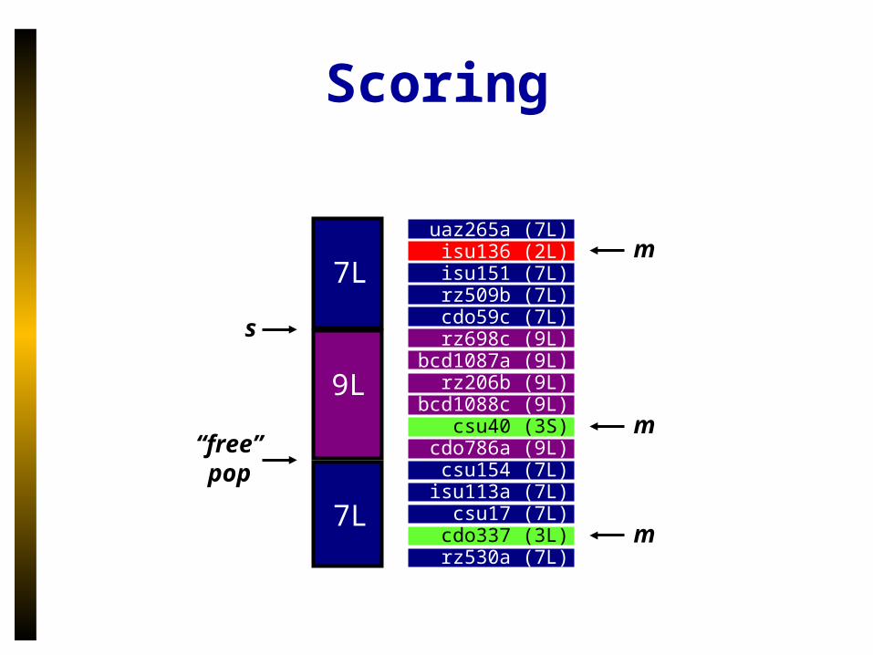
Scoring
s
9L
7L
7L
“free” pop
m
m
m
uaz265a (7L) isu136 (2L) isu151 (7L) rz509b (7L) cdo59c (7L) rz698c (9L) bcd1087a (9L) rz206b (9L) bcd1088c (9L) csu40 (3S) cdo786a (9L) csu154 (7L) isu113a (7L) csu17 (7L) cdo337 (3L) rz530a (7L)
Dynamic programming
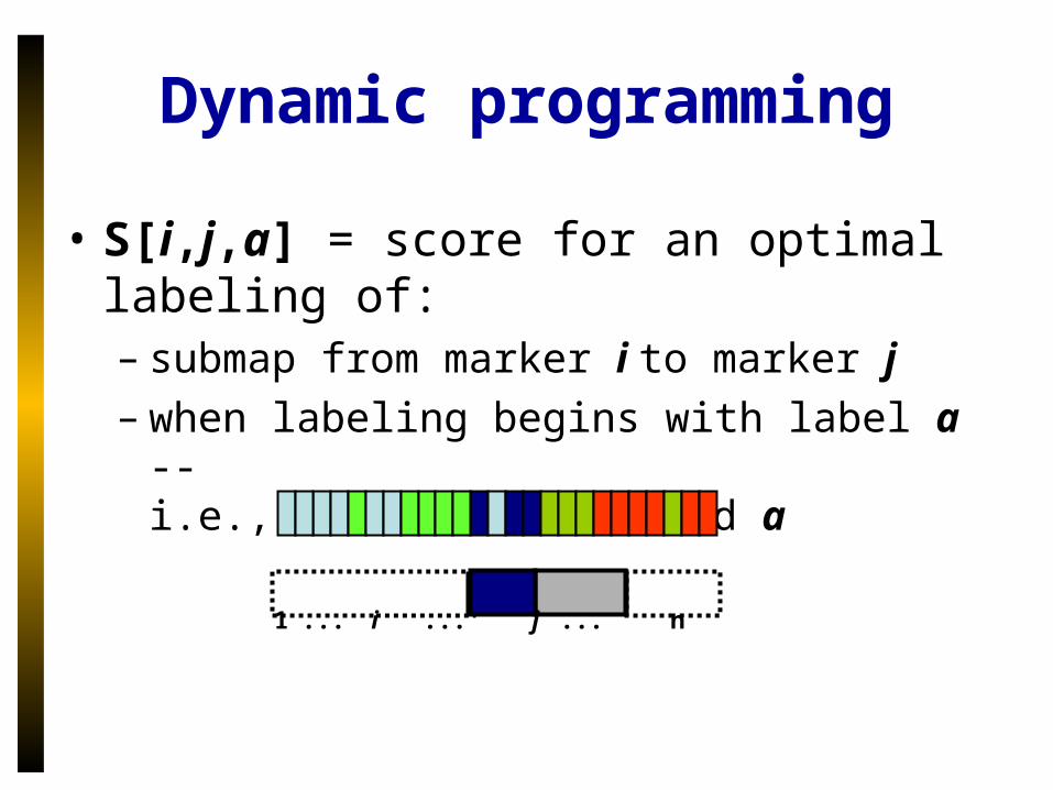
• S[i,j,a] = score for an optimal labeling of:– submap from marker i to marker j– when labeling begins with label a --
i.e., marker i is labeled a
a
1 ... i ... j ... n
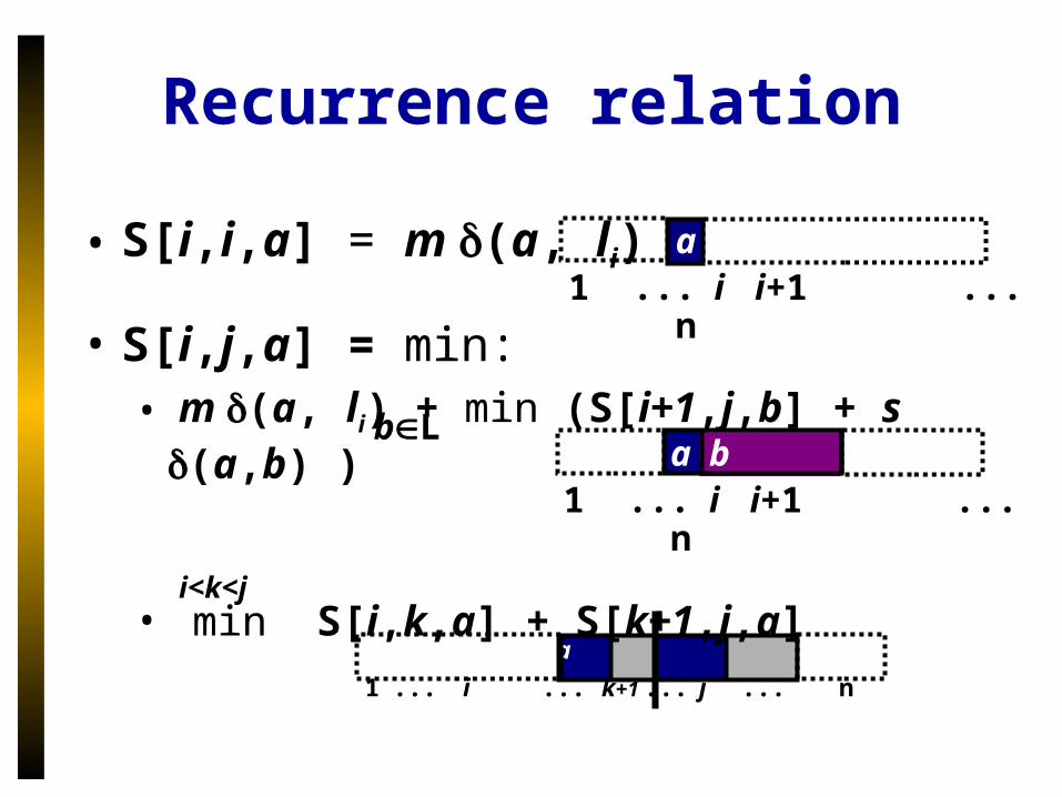
Recurrence relation
• S[i,i,a] = m (a, li)
• S[i,j,a] = min:• m (a, li) + min (S[i+1,j,b] + s (a,b) )
• min S[i,k,a] + S[k+1,j,a] i<k<j
bL
a a
1 ... i ... k+1 ... j ... n
a1 ... i i+1 ... n
a b1 ... i i+1 ... n
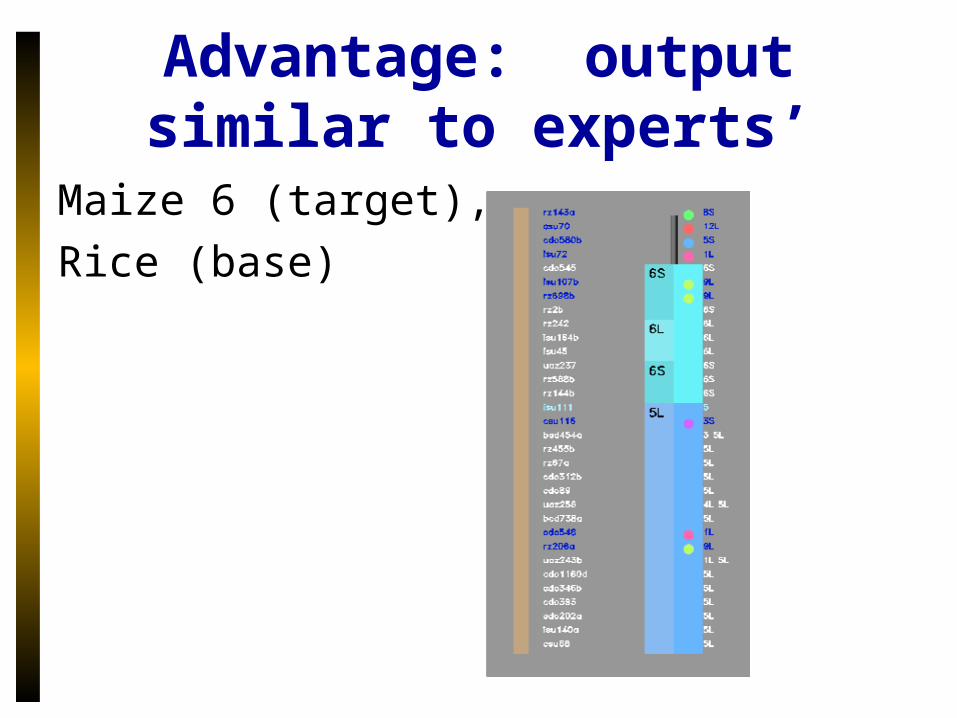
Advantage: output similar to experts’
Maize 6 (target),
Rice (base)
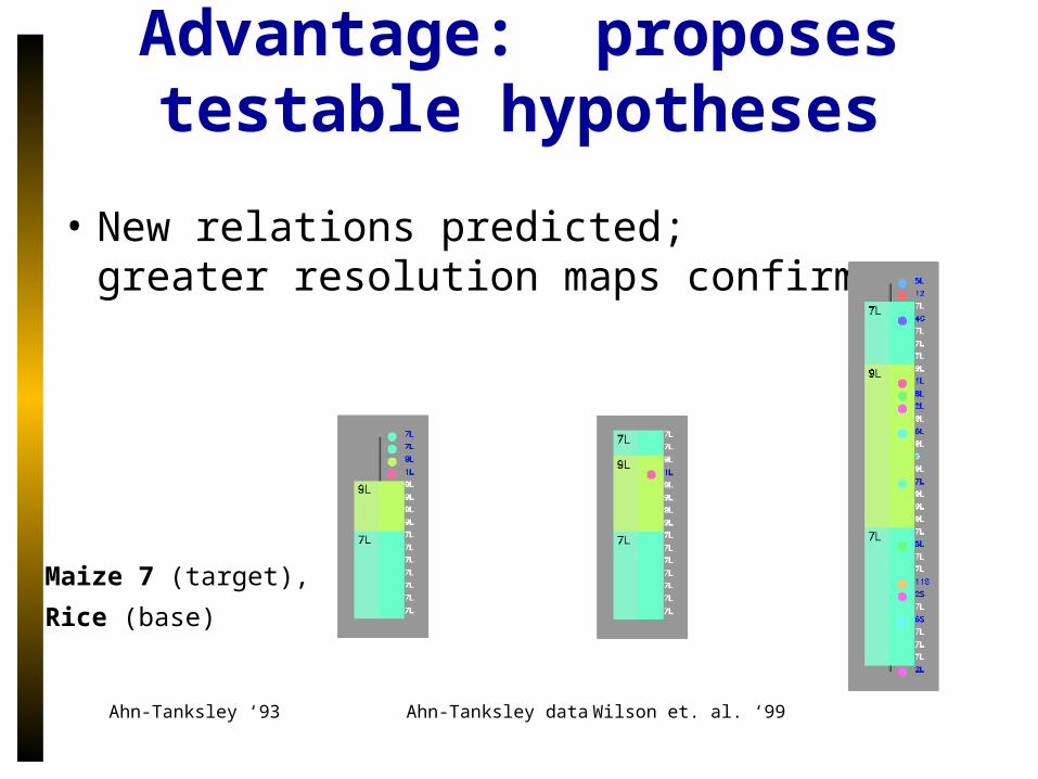
Advantage: proposes testable hypotheses
• New relations predicted;greater resolution maps confirm
Ahn-Tanksley ‘93 Ahn-Tanksley data Wilson et. al. ‘99
Maize 7 (target),
Rice (base)
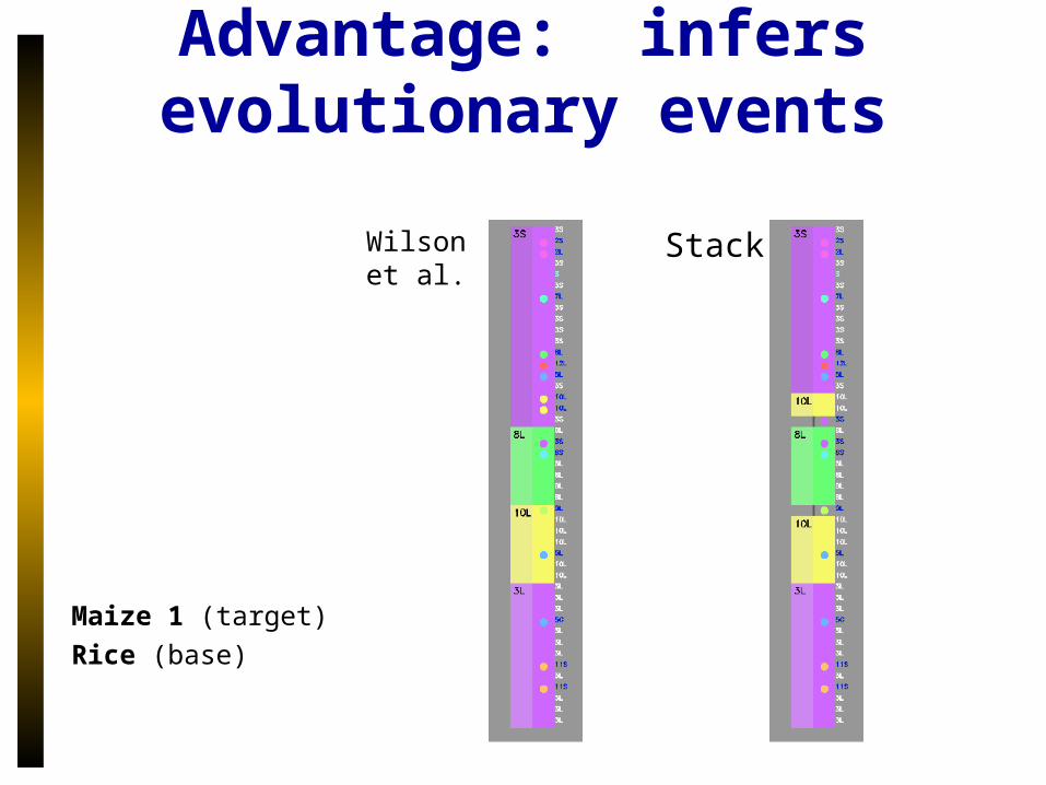
Advantage: infers evolutionary events
Maize 1 (target)
Rice (base)
Wilson et al.
Stack
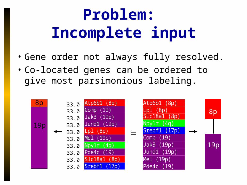
Problem: Incomplete input
• Gene order not always fully resolved.
• Co-located genes can be ordered to give most parsimonious labeling.
8p
19p
33.0 Atp6b1 (8p)33.0 Comp (19)33.0 Jak3 (19p)33.0 Jund1 (19p)33.0 Lpl (8p)33.0 Mel (19p)33.0 Npy1r (4q)33.0 Pde4c (19)33.033.0 Srebf1 (17p)
Slc18a1 (8p)
Atp6b1 (8p)Lpl (8p)
Npy1r (4q)Srebf1 (17p)Comp (19)Jak3 (19p)Jund1 (19p)Mel (19p)Pde4c (19)
Slc18a1 (8p)
=
8p
19p
33.033.033.033.033.033.033.033.033.033.0
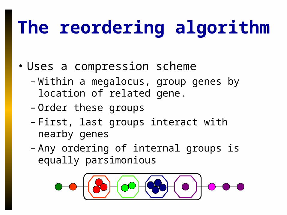
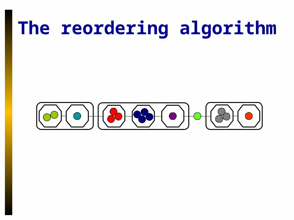
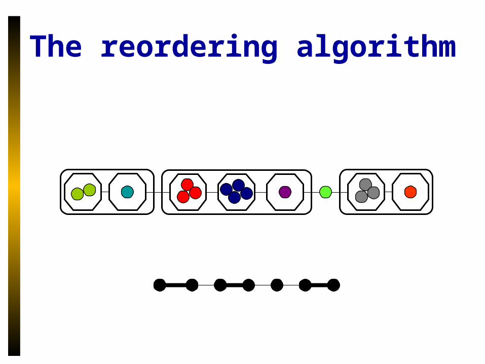
The reordering algorithm
• Uses a compression scheme– Within a megalocus, group genes by location
of related gene.– Order these groups– First, last groups interact with nearby genes– Any ordering of internal groups is equally
parsimonious
The reordering algorithm
The reordering algorithm
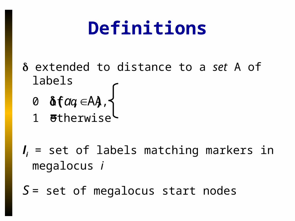
Definitions
extended to distance to a set A of labels
0 if a A,
1 otherwise
li = set of labels matching markers in megalocus i
S = set of megalocus start nodes
(a, A) =
Definitions
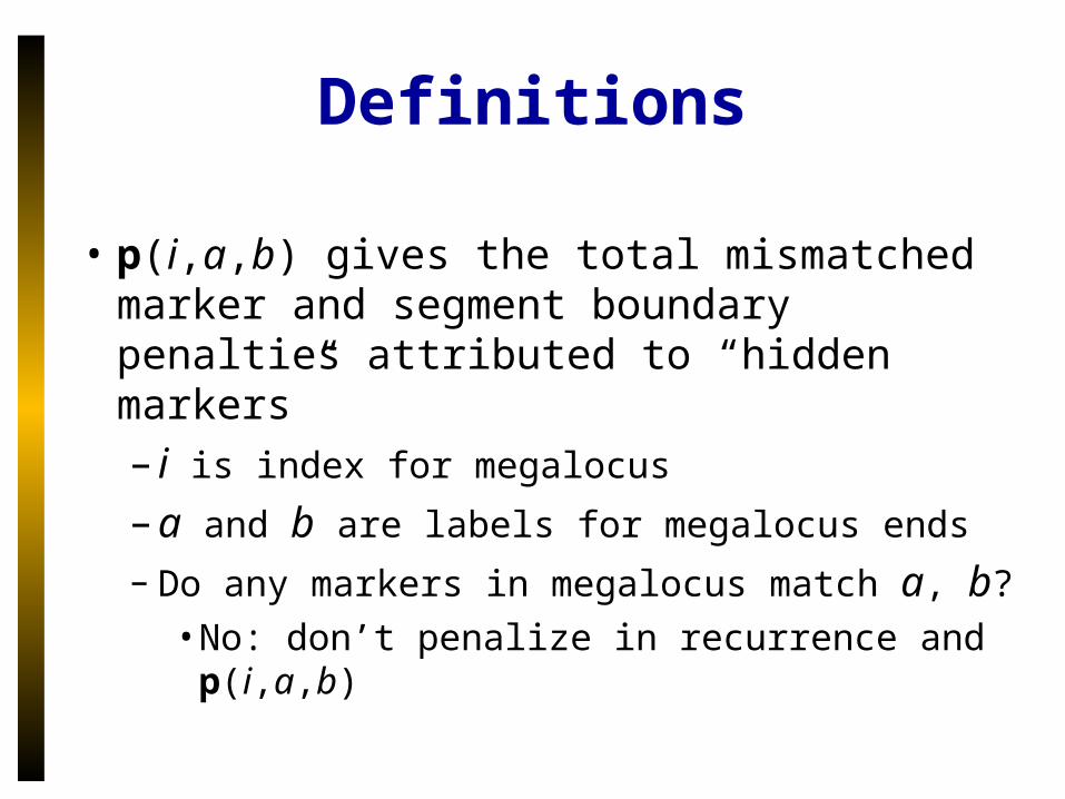
• p(i,a,b) gives the total mismatched marker and segment boundary penalties attributed to “hidden markers”– i is index for megalocus
– a and b are labels for megalocus ends
– Do any markers in megalocus match a, b?
• No: don’t penalize in recurrence and p(i,a,b)
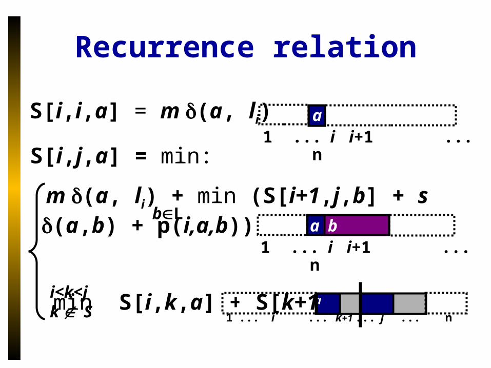
Recurrence relation
S[i,i,a] = m (a, li)
S[i,j,a] = min:
m (a, li) + min (S[i+1,j,b] + s (a,b) + p(i,a,b))
min S[i,k,a] + S[k+1,j,a] i<k<jk S
bL
a a
1 ... i ... k+1 ... j ... n
a1 ... i i+1 ... n
a b1 ... i i+1 ... n
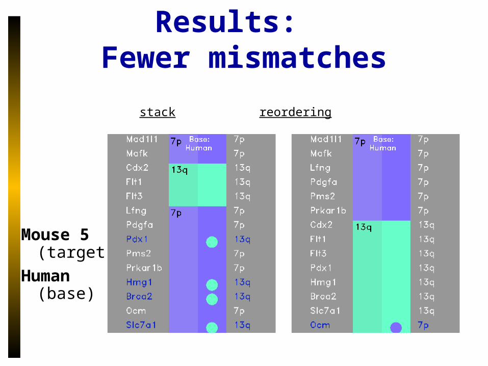
Results: Fewer mismatches
stack reordering
Mouse 5 (target)
Human (base)

Results: Mismatches placed between segments
stack reordering
Mouse 8 (target)
Human (base)
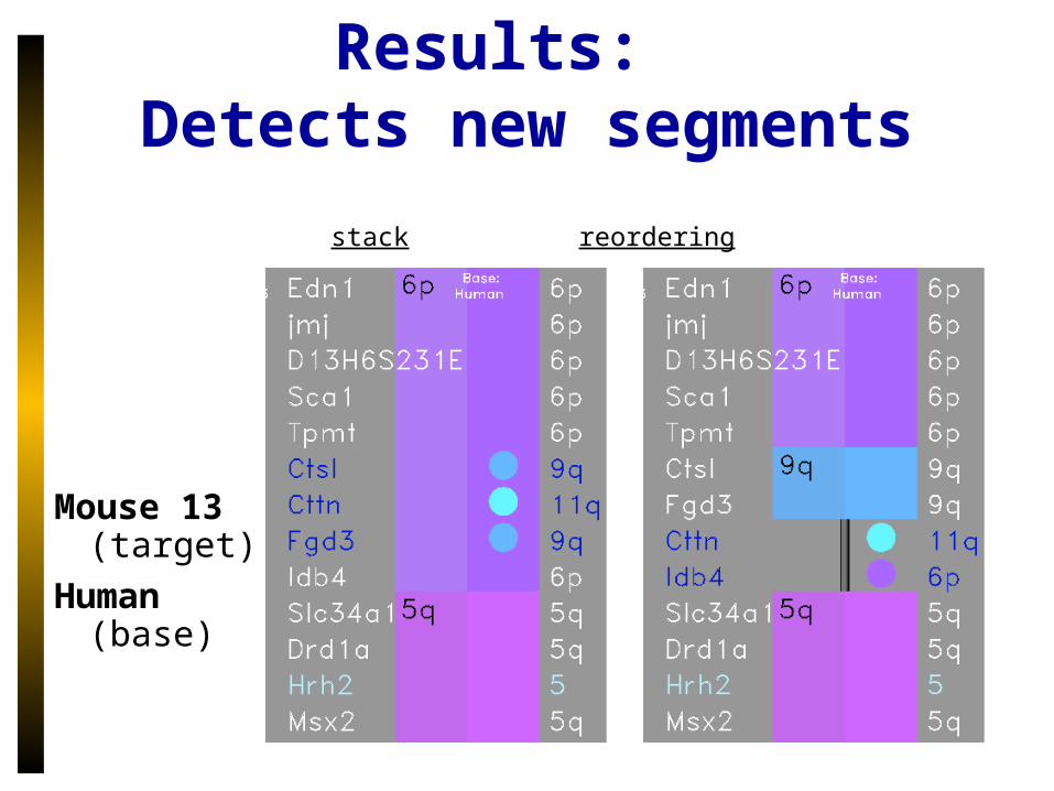
Results: Detects new segments
stack reordering
Mouse 13 (target)
Human (base)
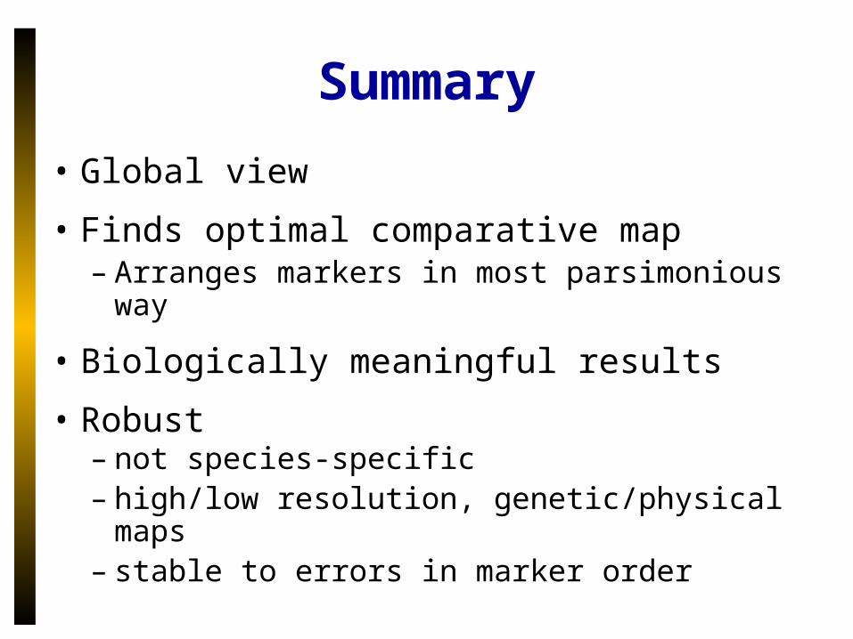
Summary
• Global view
• Finds optimal comparative map– Arranges markers in most parsimonious way
• Biologically meaningful results
• Robust– not species-specific– high/low resolution, genetic/physical maps– stable to errors in marker order


![35 [2,3]-sigmatropic rearrangements](https://img.dokumen.tips/doc/110x75/55504042b4c905b2788b48e9/35-23-sigmatropic-rearrangements.jpg)


![34 [3,3]-sigmatropic rearrangements](https://img.dokumen.tips/doc/110x75/55503fb4b4c9058f768b4911/34-33-sigmatropic-rearrangements.jpg)


