Genome characterization through a mathematical model of the genetic code

Scuola di Dottorato in Scienze Economiche e StatisticheDottorato di ricerca in

Metodologia Statistica per la Ricerca ScientificaXXV ciclo

Alm

aM

aterStudiorum

-Università

diBologna

Genome characterization through a mathematicalmodel of the genetic code: an analysis

of the whole chromosome 1 of A. thaliana

Enrico Properzi

Dipartimento di Scienze Statistiche “Paolo Fortunati”Gennaio 2013

Scuola di Dottorato in Scienze Economiche e StatisticheDottorato di ricerca in

Metodologia Statistica per la Ricerca ScientificaXXIV ciclo

Alm

aM

aterStudiorum

-Università

diBologna

Genome characterization through a mathematicalmodel of the genetic code: an analysis

of the whole chromosome 1 of A. thaliana

Enrico Properzi

Coordinatore:Prof.ssa Angela Montanari

Tutor:Prof.Rodolfo Rosa

Co-Tutor:Dott.Simone GianneriniDott.Diego L. Gonzalez

Settore Disciplinare: SECS-S/02Settore Concorsuale: 13/D1

Dipartimento di Scienze Statistiche “Paolo Fortunati”Gennaio 2013

Indice

1 Introduction 5

2 Genetic information 82.1 Central dogma of molecular biology . . . . . . . . . . . . . . . 122.2 The genetic code . . . . . . . . . . . . . . . . . . . . . . . . . 162.3 Gene structure . . . . . . . . . . . . . . . . . . . . . . . . . . 202.4 Arabidopsis thaliana as a model organism . . . . . . . . . . . . 21

3 A mathematical model for the genetic code 233.1 Mathematical structure of the code . . . . . . . . . . . . . . . 23

3.1.1 Degeneracy and redudancy . . . . . . . . . . . . . . . . 253.1.2 Non-power binary representation of the genetic code . 273.1.3 A hiearchy of symmetries . . . . . . . . . . . . . . . . . 313.1.4 Dichotomic classes for codons . . . . . . . . . . . . . . 35

4 Descriptive analysis 404.1 Base distribution . . . . . . . . . . . . . . . . . . . . . . . . . 444.2 Percentage of dichotomic classes . . . . . . . . . . . . . . . . . 46

4.2.1 Normal sequences . . . . . . . . . . . . . . . . . . . . . 464.2.2 Complementary sequences . . . . . . . . . . . . . . . . 504.2.3 Reverted sequences . . . . . . . . . . . . . . . . . . . . 514.2.4 Keto/Amino global transformation sequences . . . . . 514.2.5 Purine/Pyrimidine global transformation sequences . . 524.2.6 Comments . . . . . . . . . . . . . . . . . . . . . . . . . 53

4.3 Independence test . . . . . . . . . . . . . . . . . . . . . . . . . 544.3.1 Comments . . . . . . . . . . . . . . . . . . . . . . . . . 57

4.4 Conclusions . . . . . . . . . . . . . . . . . . . . . . . . . . . . 60

5 Discriminating different portions of the genome 625.1 Classification through Logistic Regression . . . . . . . . . . . . 625.2 Sequence classification of A.thaliana chromosome 1 . . . . . . 65

2

5.2.1 Exons vs Introns . . . . . . . . . . . . . . . . . . . . . 675.2.2 CDS vs. Long introns . . . . . . . . . . . . . . . . . . . 705.2.3 Exons vs. CDS . . . . . . . . . . . . . . . . . . . . . . 725.2.4 Genes vs. Intergenes . . . . . . . . . . . . . . . . . . . 745.2.5 Exons vs. UTRs . . . . . . . . . . . . . . . . . . . . . . 765.2.6 Introns vs. UTRs . . . . . . . . . . . . . . . . . . . . . 78

5.3 Comments . . . . . . . . . . . . . . . . . . . . . . . . . . . . . 80

6 Dependence analysis 816.1 Dependence measures . . . . . . . . . . . . . . . . . . . . . . . 82

6.1.1 Chi-squared test for independence . . . . . . . . . . . . 846.1.2 Mutual information . . . . . . . . . . . . . . . . . . . . 876.1.3 Sρ . . . . . . . . . . . . . . . . . . . . . . . . . . . . . 89

6.2 Sequence analysis . . . . . . . . . . . . . . . . . . . . . . . . . 926.2.1 Results . . . . . . . . . . . . . . . . . . . . . . . . . . . 956.2.2 Comparison between indexes . . . . . . . . . . . . . . . 1026.2.3 Comments . . . . . . . . . . . . . . . . . . . . . . . . . 102

6.3 Multiple testing problem . . . . . . . . . . . . . . . . . . . . . 1066.3.1 Statistical Solutions to the Multiple Testing Problem . 1086.3.2 Related problems . . . . . . . . . . . . . . . . . . . . . 110

7 Conclusions 112

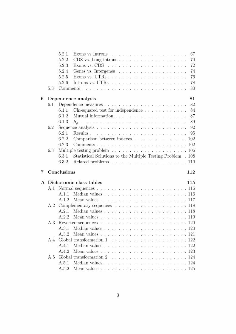
A Dichotomic class tables 115A.1 Normal sequences . . . . . . . . . . . . . . . . . . . . . . . . . 116

A.1.1 Median values . . . . . . . . . . . . . . . . . . . . . . . 116A.1.2 Mean values . . . . . . . . . . . . . . . . . . . . . . . . 117

A.2 Complementary sequences . . . . . . . . . . . . . . . . . . . . 118A.2.1 Median values . . . . . . . . . . . . . . . . . . . . . . . 118A.2.2 Mean values . . . . . . . . . . . . . . . . . . . . . . . . 119

A.3 Reverted sequences . . . . . . . . . . . . . . . . . . . . . . . . 120A.3.1 Median values . . . . . . . . . . . . . . . . . . . . . . . 120A.3.2 Mean values . . . . . . . . . . . . . . . . . . . . . . . . 121

A.4 Global transformation 1 . . . . . . . . . . . . . . . . . . . . . 122A.4.1 Median values . . . . . . . . . . . . . . . . . . . . . . . 122A.4.2 Mean values . . . . . . . . . . . . . . . . . . . . . . . . 123

A.5 Global transformation 2 . . . . . . . . . . . . . . . . . . . . . 124A.5.1 Median values . . . . . . . . . . . . . . . . . . . . . . . 124A.5.2 Mean values . . . . . . . . . . . . . . . . . . . . . . . . 125

3

B Distributions 126B.1 Dichotomic classes distributions . . . . . . . . . . . . . . . . . 127B.2 Base distribution . . . . . . . . . . . . . . . . . . . . . . . . . 143

4

Capitolo 1

Introduction

In this thesis work I would like to combine my different skills as a biotechno-logist and as a statistician. I decided to analyze, from a mathematical pointof view, the genome of the whole chromosome 1 of a simple plant organi-sm, Arabidopsis thaliana (A.thaliana), that represents a model for molecularbiology and genetic studies.

The discovery of the genetic code, a universal translation table that linksthe world of nucleic acids to the world of proteins, led scientists to focus onsequencing the entire genomes of different organisms. The Human GenomeProject succeeded in sequencing the whole human genome in 2001 [38, 54]and triggered a strong hype on the possibility of diagnosing and treating ma-ny serious diseases. However, after ten years, it looks like the expectationshave not been met. The recent article by S.S. Hall published on Scienti-fic American: “Revolution Postponed: Why the Human Genome Project HasBeen Disappointing” is emblematic: In fact its subtitle states: “The HumanGenome Project has failed so far to produce the medical miracles that scien-tists promised. Biologists are now divided over what, if anything, went wrong- and what needs to happen next”.

The whole genetic information is passed from a parent cell to two or moredaughter cells through the process of cell division. The main concern of celldivision is the maintenance of the genome of the original cell. Before divisioncan occur, the genetic information must be replicated and the duplicatedgenome is separated cleanly between cells. During DNA replication severalerrors may occur. Some of these errors have no effect on the life of the cell,while others can result in growth defects, cell death or cancer. A permanentchange in the DNA sequence of a gene is called mutation. [44, 45].

Mutations occasionally occur within cells as they divide and can affectthe behaviour of cells, sometimes causing them to grow and divide morefrequently. Several biological mechanisms can stop this process: biochemical

5

signals can cause inappropriately dividing cells to die. Sometimes additionalmutations make cells ignore these messages. Most dangerously, a mutationmay give a cell a selective advantage, allowing it to divide more vigorouslythan its neighbours and to become a founder of a growing mutant clone.Since mutations may occur because of errors during DNA replication, thestudy of error detection/correction mechanism in such process could be ofkey importance for understanding the onset of different serious pathologies,among with there is cancer.

In biology, a reading frame is a way of breaking a sequence of nucleo-tides in DNA or RNA into three letter codons which can be translated inamino acids. There are 3 possible reading frames in an DNA strand: eachreading frame corresponds to starting at a different alignment. Usually, thereis only one correct reading frame. Moreover, error detection and correctionmechanisms are strictly involved with frame recognition. [39]

In this work I study the features of different portions of the genome ofA.thaliana, by using a recently developed mathematical model for the ge-netic code [16, 18, 17]. I use the information of dichotomic classes, binaryvariables naturally derived from the above mentioned model, in order to as-sess different behaviours between coding and non coding sequences. In par-ticular I analyze the role of frame. So far, the mathematical model of thegenetic code has been used to investigate only some proteins of different ori-gin [19, 20, 21, 22, 23]. Now I apply it to a whole chromosome of a single(and well-known) organism: A.thaliana. It has many advantages for genomeanalysis: a small size, a short generation time and relatively small nuclear ge-nome. These advantages promoted the growth of a scientific community thathas investigated the biological processes of A.thaliana and has characterizedmany genes [50].

Finally, since the existence of a coding mechanism for error correctionand detection implies some kind of dependence inside data, I want finallyto study the presence of dependence structure, related to dichotomic classes,within different portion of the genome. It could be useful in order to developalternative methods to understand error detection and correction mechanismsinvolved in the translation process.

The thesis is organized as follows: in chapter 1 I introduce the basic conceptand terminology of genetics and the model organism A.thaliana. In chapter 2I describe the salient features of the mathematical model. In chapter 3 I per-form a descriptive statistical analysis on the data set; moreover, I implementand apply a test for independence based on dichotomic classes. In chapter 4

6

I describe logistic regression models built in order to discriminate betweendifferent portions of the genome. In chapter 5 I use three different measuresof dependence (χ2, Sρ and mutual information) in order to assess if there areshort-range dependence structure related to dichotomic class within differentportions of the genome. Finally I discuss the results.

7

Capitolo 2

Genetic information

Genetics is the science of genes, heredity, and variation in living organisms[27]. It deals with the molecular structure and function of genes. Since genesare universal to living organisms, genetics can be applied to the study ofall living systems, from viruses and bacteria, through plants and domesticanimals, to humans (as in medical genetics).

The genetic information is carried by genes segments of DNA (deoxy-ribonucleic acid) located on chromosomes. They exist in alternative formscalled alleles that determine distinct traits which can be passed on fromparents to offspring. The process by which genes are transmitted was disco-vered by Gregor Mendel and formulated in what is known as Mendel’s lawof segregation.

DNA is a self-replicating nucleic acid which is present in nearly all livingorganisms as the main constituent of chromosomes. It is the carrier of geneticinformation.

DNA The molecular basis of genes is DNA. Each molecule of DNA consistsof two strands coiled round each other to form a double helix, a structure likea spiral ladder. DNA is a polymer. The monomer units of DNA are nucleoti-des, and the polymer is known as a polynucleotide. Each nucleotide consistsof a 5-carbon sugar (deoxyribose), a nitrogen containing base attached to thesugar, and a phosphate group (see Figure 2). There are four different typesof nucleotides found in DNA, differing only in the nitrogenous base. The fournucleotides are given one letter abbreviations as shorthand for the four bases.

• A is for adenine

• G is for guanine

• C is for cytosine

8

• T is for thymine

Figura 2.1: DNA molecule structure(from http://commons.wikimedia.org, under Creative Commons)

Adenine and guanine are purines while cytosine and thymine are pyrimi-dines. Purines are the larger of the two types of bases found in DNA; theyhave two nitrogen-containing rings while pyrimidines have only one.

A nucleoside is one of the four DNA bases covalently attached to theC1’ position of a sugar. The sugar in deoxynucleosides is 2’-deoxyribose. Anucleotide is a nucleoside with one or more phosphate groups covalentlyattached to the 3’- and/or 5’-hydroxyl group (see Figure 2).

The DNA backbone is a polymer with an alternating sugar-phosphatesequence. The deoxyribose sugars are joined at both the 3’-hydroxyl and5’-hydroxyl groups to phosphate groups in ester links, also known as pho-sphodiester bonds. Chain has a direction (known as polarity), 5’- to 3’- fromtop to bottom and A, G, C, and T bases can extend away from chain, andstack atop each other.The bases combine in specific pairs (A/T and C/G)sothat the sequence on one strand of the double helix is complementary to thaton the other: it is the specific sequence of bases which constitutes the geneticinformation. [27]

9

Features of the DNA double helix:

• Two DNA strands form a helical spiral, winding around a helix axis ina right-handed spiral

• The two polynucleotide chains run in opposite directions

• The sugar-phosphate backbones of the two DNA strands wind aroundthe helix axis like the railing of a spiral staircase

• The bases of the individual nucleotides are on the inside of the helix,stacked on top of each other like the steps of a spiral staircase.

• Within the DNA double helix, A forms 2 hydrogen bonds with T on theopposite strand, and G forms 3 hydrogen bonds with C on the oppositestrand. For this reason and G are called Strong bases (S) while T andA are called Weak (W).

Genes are arranged linearly along long chains of DNA base-pair sequen-ces. In bacteria, each cell usually contains a single circular genophore, whileeukaryotic organisms (including plants and animals) have their DNA arran-ged in multiple linear chromosomes. These DNA strands are often extremelylong; the largest human chromosome (chromosome 1), for example, is about247 million base pairs in length.[26]

All living organisms can be sorted into one of two groups depending onthe fundamental structure of their cells. These two groups are the prokaryotesand the eukaryotes:

• Prokaryotes are organisms made up of cells that lack a cell nucleusor any membrane-encased organelles. This means the genetic materialDNA in prokaryotes is not bound within a nucleus. Additionally, theDNA is less structured in prokaryotes than in eukaryotes. In prokaryo-tes, DNA is a single loop. In eukaryotes, DNA is organized into chromo-somes. Most prokaryotes are made up of just a single cell (unicellular)but there are a few that are made of collections of cells (multicellular).Scientists have divided the prokaryotes into two groups, the Bacteriaand the Archaea.

• Eukaryotes are organisms made up of cells that possess a membrane-bound nucleus (that holds genetic material) as well as membrane-boundorganelles. Genetic material in eukaryotes is contained within a nucleuswithin the cell and DNA is organized into chromosomes. Eukaryoticorganisms may be multicellular or single-celled organisms. All animalsare eukaryotes. Other eukaryotes include plants, fungi, and protists.

10

Figura 2.2: Components of a DNA molecule(from: http://www.nature.com/scitable)

11

2.1 Central dogma of molecular biologyThe central dogma of molecular biology describes the flow of genetic infor-mation within a biological system. It was first stated by Francis Crick in 1958and re-stated in a Nature paper published in 1970. [7]

The central dogma of molecular biology deals with the detailed transferof sequential information. It states, as Marshall Nirenberg said, DNA makesRNA makes protein meaning that information is transferred from DNA toRNA and from RNA to proteins and not in the opposite sense.

The dogma is a framework for understanding the transfer of sequence in-formation between sequential information-carrying biopolymers, in the mostcommon or general case, in living organisms. There are 3 major classes ofsuch biopolymers: DNA and RNA and protein. DNA, deoxyribonucleic acid,and RNA, ribonucleic acid, are molecules that hold the genetic informationof each cell. The DNA strands store information, while the RNA moleculestake the information from the DNA, transfer it to different places in the cell,and decode or read the information. RNA molecules are similar to DNA onesexcept for:

• The sugar present in the backbone is ribose instead of deoxyribose

• The nucleobase thymine (T) is substituted by Uracil (U)

• RNA molecules are formed by a single strand

Proteins, instead, are large biological molecules consisting of one or morechains of amino acids. [42]

The flow of biological information is:

• DNA can be copied to DNA (DNA replication),

• DNA information can be copied into mRNA (transcription), and

• proteins can be synthesized using the information in mRNA as a tem-plate (translation).

Replication It is the process in which a cell makes an exact copy of its ownDNA (copy DNA → DNA). Replication occurs in the step of cell divisioncycle during which the genetic information is transferred from the mother-cell to the daughter-cell. Replication begins with local decondensation andseparation of the double DNA helices, so that the DNA molecule becomesaccessible for enzymes that make a complementary copy of each strand (seeFigure 2.1).During DNA replication, it takes place DNA errors control.

12

Figura 2.3: DNA replication(from http://commons.wikimedia.org, under Creative Commons)

13

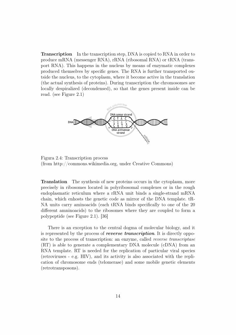
Transcription In the transcription step, DNA is copied to RNA in order toproduce mRNA (messenger RNA), rRNA (ribosomal RNA) or tRNA (trans-port RNA). This happens in the nucleus by means of enzymatic complexesproduced themselves by specific genes. The RNA is further transported ou-tside the nucleus, to the cytoplasm, where it become active in the translation(the actual synthesis of proteins). During transcription the chromosomes arelocally despiralized (decondensed), so that the genes present inside can beread. (see Figure 2.1)

Figura 2.4: Transcription process(from http://commons.wikimedia.org, under Creative Commons)

Translation The synthesis of new proteins occurs in the cytoplasm, moreprecisely in ribosomes located in polyribosomal complexes or in the roughendoplasmatic reticulum where a rRNA unit binds a single-strand mRNAchain, which enhosts the genetic code as mirror of the DNA template. tR-NA units carry aminoacids (each tRNA binds specifically to one of the 20different amninoacids) to the ribosomes where they are coupled to form apolypeptide (see Figure 2.1). [36]

There is an exception to the central dogma of molecular biology, and itis represented by the process of reverse transcription. It is directly oppo-site to the process of transcription: an enzyme, called reverse transcriptase(RT) is able to generate a complementary DNA molecule (cDNA) from anRNA template. RT is needed for the replication of particular viral species(retroviruses - e.g. HIV), and its activity is also associated with the repli-cation of chromosome ends (telomerase) and some mobile genetic elements(retrotransposons).

14

Figura 2.5: Translation processfrom: http://hyperphysics.phy-astr.gsu.edu/hbase/hframe.html

15

2.2 The genetic codeGenetic information, represented by genes, is used by organisms to create allthe proteins necessary for their metabolism. The genetic code is the dictio-nary used by the cell to translate a sequence of codons (triplets or bases) ofRNA in a sequence of amino acids during the translation process. Almost allliving organisms use the same genetic code, called the standard genetic code(see Table 3.1), but many slight variants have been discovered. There arevarious alternative mitochondrial codes, and small variants in some membersof bacteria and archaea.

Despite these differences, all known naturally-occurring codes are verysimilar to each other, and the coding mechanism is the same for all organisms:it implies three-base codons, tRNA, ribosomes, reading the code in the samedirection and translating the code three letters at a time into sequences ofamino acids.

The ribosome facilitates the decoding process by inducing the binding oftRNAs with complementary anticodon sequences to that of the mRNA. ThetRNAs carry specific amino acids that are chained together into a polypep-tide as the mRNA passes through and is read by the ribosome in a fashionreminiscent to that of a stock ticker and ticker tape. Each codon correspondsto a specific amino acid, then it is said that the codon encodes that specificaminoacid in the genetic code. [8] [43]

The RNA is made of four bases: adenine (A), guanine (G), cytosine (C)and uracil (U) (in DNA uracil is replaced by thymine (T)). There are the-refore 43 = 64 possible codons. 61 of them encode amino acids, while theremaining three (UAA, UAG, UGA) encode stop signals, that is, at whatpoint the assembly of the polypeptide chain should be stopped. Because theamino acids that contribute to the formation of proteins are 20, they generallyare encoded by more than one codon.

Therefore genetic code is said to be degenerate and different codons thatencode the same amino acid are synonymous. For example, the sequenceof RNA UUUACACAG consists of three codons, UUU, ACA, CAG, whichcorrespond to the amino acids Phenylalanine (Phe), Threonine (Thr) andGlutamine (Gln). Protein synthesis applied to this sequence would then ge-nerate the tripeptide Phe-Thr-Gln. Therefore, we can say that the geneticcode connects the language of nucleic acids and the language of proteins. InTable 3.1 codons are displayed into quartets: groups of codons sharing thefirst two bases.

Not all genetic information is stored using the genetic code. In all organi-sms, DNA contains regulatory sequences: intergenic segments, chromosomalstructural areas, and other non-coding DNA that can contribute greatly to

16

UUU Phe UCU Ser UAU Tyr UGU CysUUC Phe UCC Ser UAC Tyr UGC CysUUA Leu UCA Ser UAA Stp UGA StpUUG Leu UCG Ser UAG Stp UGG Trp

CUU Leu CCU Pro CAU His CGU ArgCUC Leu CCC Pro CAC His CGC ArgCUA Leu CCA Pro CAA Gln CGA ArgCUG Leu CCG Pro CAG Gln CGG Arg

AUU Ile ACU Thr AAU Asn AGU SerAUC Ile ACC Thr AAC Asn AGC SerAUA Ile ACA Thr AAA Lys AGA ArgAUG Met ACG Thr AAG Lys AGG Arg

GUU Val GCU Ala GAU Asp GGU GlyGUC Val GCC Ala GAC Asp GGC GlyGUA Val GCA Ala GAA Glu GGA GlyGUG Val GCG Ala GAG Glu GGG Gly

Tabella 2.1: Standard genetic code

17

Figura 2.6: RNA codons (from http://commons.wikimedia.org, underCreative Commons)

18

phenotype. Those elements operate under sets of rules that are distinct fromthe codon-to-amino acid paradigm underlying the genetic code.[?]

Sequence reading frame A codon is defined by the initial nucleotide fromwhich translation starts. For example, the previous sequence UUUACACAG,if read from the first position, contains the codons UUU, ACA, and CAG;and, if read from the second position, it contains the codons UUA and CAC;if read starting from the third position, UAC and ACA. Every sequencecan, thus, be read in three reading frames, each of which will produce adifferent amino acid sequence (in the given example, Phe-Thr-Gln, Leu-His,or Tyr-Thr, respectively). With double-stranded DNA, there are six possiblereading frames, three in the forward orientation on one strand and threereverse on the opposite strand. The actual frame in which a protein sequenceis translated is defined by a start codon, usually the first AUG codon in themRNA sequence. [43]

Start/stop codons Translation starts with a chain initiation codon (startcodon). Unlike stop codons, the codon alone is not sufficient to begin theprocess. Nearby sequences (such as the Shine-Dalgarno sequence in E.coli)and initiation factors are also required to start translation. The most commonstart codon is AUG, which is read as methionine (Met) or, in bacteria, asformylmethionine. The three stop codons are: UAG, UGA and UAA. Stopcodons are also called termination or nonsense codons. They signal releaseof the nascent polypeptide from the ribosome because there is no cognatetRNA that has anticodons complementary to these stop signals, and so arelease factor binds to the ribosome instead.[?]

Mutations During the process of DNA replication, errors occasionally oc-cur in the polymerization of the second strand. These errors, called muta-tions, can have an impact on the phenotype of an organism, especially ifthey occur within the protein coding sequence of a gene. Error rates areusually very low (1 error in every 10-100 million bases) due to the proofrea-ding ability of DNA polymerases.[27][?] Missense mutations and nonsensemutations are examples of point mutations. Clinically important missensemutations generally change the properties of the coded amino acid residuebetween being basic, acidic polar or non-polar, whereas nonsense mutationsresult in a stop codon. Mutations that disrupt the reading frame sequenceby indels (insertions or deletions) of a non-multiple of 3 nucleotide bases areknown as frameshift mutations. These mutations usually result in a comple-tely different translation from the original, and are also very likely to cause

19

a stop codon to be read, which truncates the creation of the protein. Thesemutations may impair the function of the resulting protein. Although mostmutations that change protein sequences are harmful or neutral, some mu-tations have a positive effect on an organism. These mutations may enablethe mutant organism to withstand particular environmental stresses betterthan wild-type organisms, or reproduce more quickly. In these cases a mu-tation will tend to become more common in a population through naturalselection.[43]

2.3 Gene structureThere are two general types of gene in the human genome: non-coding RNAgenes and protein-coding genes. Non-coding RNA genes represent 2-5 percent of the total and encode functional RNA molecules. Many of these RNAsare involved in the control of gene expression, particularly protein synthe-sis. They have no overall conserved structure. Protein-coding genes representthe majority of the total and are expressed in two stages: transcription andtranslation. They show incredible diversity in size and organisation and ha-ve no typical structure. There are, however, several conserved features. Theboundaries of a protein-encoding gene are defined as the points at whichtranscription begins and ends. The core of the gene is the coding region,which contains the nucleotide sequence that is eventually translated into thesequence of amino acids in the protein. The coding region begins with the ini-tiation codon, which is normally AUG. It ends with one of three terminationcodons: UAA, UAG or UGA. On either side of the coding region are DNAsequences that are transcribed but are not translated. These untranslatedregions or non-coding regions often contain regulatory elements that controlprotein synthesis. Both the coding region and the untranslated regions maybe interrupted by introns. Most human genes are divided into exons andintrons. The exons are the sections that are found in the mature transcript(messenger RNA), while the introns are removed from the primary transcriptby a process called splicing. [39]

Summarizing, eukaryotic gene structure is shown in the following figure:

20

We can recognize:

• Genes: regions of a genomic sequence corresponding to a unit of in-heritance. They are formed by regulatory regions, transcribed regions,and/or other functional sequence regions.

• Exons: portions of a gene that are transcribed into mRNA and thentranslated into a protein. Each gene can contain one or more exons.

• CDS: portions of a gene that encode for a given protein. It is formedby joining exons (one or more) within a gene.

• Introns: portions of a gene that are transcribed but not translated.

• Intergenes: sequences between a gene and the following one.

• UTR: portions of mRNA that precede the codon that begins transla-tion (AUG) (5’UTR) and follow the termination codon (3’ UTR)

• Regulatory regions: portions of a gene, with regulatory function, thatprecede (upstream) and follow (downstream) the fragment transcriptedinto mRNA

2.4 Arabidopsis thaliana as a model organismAlthough geneticists originally studied inheritance in a wide range of organi-sms, researchers began to specialize in studying the genetics of a particularsubset of organisms. The fact that significant research already existed fora given organism would encourage new researchers to choose it for furtherstudy, and so eventually a few model organisms became the basis for mostgenetics research.Common research topics in model organism genetics inclu-de the study of gene regulation and the involvement of genes in developmentand cancer. Organisms were chosen, in part, for convenience-short generationtimes and easy genetic manipulation. Widely used model organisms include

21

the gut bacterium Escherichia coli, the plant Arabidopsis thaliana, baker’syeast Saccharomyces cerevisiae, the nematode Caenorhabditis elegans, thecommon fruit fly Drosophila melanogaster, and the common house mouseMus musculus.

Arabidopsis thaliana (A. thaliana) is a small flowering plant native toEurope, Asia, and northwestern Africa. A spring annual with a relativelyshort life cycle, A. thaliana is popular as a model organism in plant biologyand genetics. A. thaliana has a rather small genome, only 157 megabase pairs(Mbp) and five chromosomes [50]. Arabidopsis was the first plant genome tobe sequenced, and is a popular tool for understanding the molecular biologyof many plant traits. By the beginning of 1900s, A.thaliana began to be usedin some developmental studies. It plays the role in plant biology that miceand fruit flies (Drosophila) play in animal biology. Although A.thaliana haslittle direct significance for agriculture, it has several traits that make it auseful model for understanding the genetic, cellular, and molecular biologyof flowering plants.

The small size of its genome makes A. thaliana useful for genetic mappingand sequencing. It was the first plant genome to be sequenced, completed in2000 by the Arabidopsis Genome Initiative.[35] The most up-to-date versionof the A.thaliana genome is maintained by the Arabidopsis Information Re-source (TAIR). Much work has been done to assign functions to its 27,000genes and the 35,000 proteins they encode.[50]

22

Capitolo 3

A mathematical model for thegenetic code

The genetic code is the dictionary used by the cell to translate a sequence ofcodons (triplets or bases) of RNA in a sequence of amino acids during thetranslation process. In Table 3.1 codons are displayed into quartets: groups ofcodons sharing the first two bases. Since 64 codons encode for 20 amino acidsand the stop signal, some amino acids are necessarily encoded by more thanone codon. This fact determines the properties of redundancy and degeneracytypical of the genetic code.

Why amino acids are not represented in a unique way? And why the levelof degeneracy is different between amino acids?

3.1 Mathematical structure of the codeIn order to try to answer these questions we could resort to informationtheory, a branch of applied mathematics involving the quantification of in-formation. A key measure of information is known as entropy.In informationtheory, entropy is a measure of the uncertainty associated with a random va-riable. In this context, the term usually refers to the Shannon entropy, whichquantifies the expected value of the information contained in a message,usually in units such as bits. In this context, a “message” means a speci-fic realization of the random variable and implies the presence of a term ofuncertainty (error).

Considering genetic code as a communication system allow us to applyinformation theory concept. Therefore we can state that it is not a free-errorsystem. Errors, which occur mainly during the transmission phase, can bedetected and then corrected at the time of decoding the message. Gonzalez

23

Tabella 3.1: Standard genetic code

UUU Phe UCU Ser UAU Tyr UGU CysUUC Phe UCC Ser UAC Tyr UGC CysUUA Leu UCA Ser UAA Stp UGA StpUUG Leu UCG Ser UAG Stp UGG Trp

CUU Leu CCU Pro CAU His CGU ArgCUC Leu CCC Pro CAC His CGC ArgCUA Leu CCA Pro CAA Gln CGA ArgCUG Leu CCG Pro CAG Gln CGG Arg

AUU Ile ACU Thr AAU Asn AGU SerAUC Ile ACC Thr AAC Asn AGC SerAUA Ile ACA Thr AAA Lys AGA ArgAUG Met ACG Thr AAG Lys AGG Arg

GUU Val GCU Ala GAU Asp GGU GlyGUC Val GCC Ala GAC Asp GGC GlyGUA Val GCA Ala GAA Glu GGA GlyGUG Val GCG Ala GAG Glu GGG Gly

24

et al. [19] investigated the existence of error-detection and correction mecha-nisms in the genetic machinery based on a particular mathematical modelof the genetic code. This model can encode each nucleotidic sequence intothree binary strings of different meaning; these strings show some interestingcorrelation patterns that enforce the hypothesis of deterministic error andcorrection mechanisms. In the following pages we explain the features of thismathematical model.

3.1.1 Degeneracy and redudancy

The genetic code is a surjective (all amino acids are encoded by at least onecodon) and non-injective (some amino acids are degenerate) function betweentwo sets of different cardinality. We can say that the codon set is the domainand the amino acids set the codomain. This implies the degeneration of thecode.

Gonzalez [16, 18, 17] proposed a model that explains the degeneracy of thegenetic code based on a non-power number representation system. This ap-proach describes the structure of the genetic code from a mathematical pointof view and allows the analysis of degeneracy and redundancy properties ontwo related levels:• the distribution of degeneration (the number of codons that code for

each amino acid)

• the distribution of codons (codons assigned to each specific amino acid)The code is degenerate from the amino acids point of view: a given ami-

no acid can indeed be encoded by more than one codon. The redundancy,however, is a property that concerns the codons: a set of triplets that encodethe same amino acid is said to be redundant. Degeneracy and redundancyare still described by the numerical quantities that define the respective sub-sets: tyrosine is a degeneracy-2 amino acid because it is encoded by a set oftwo redundant codons (UAU, UAC). Tables 3.2 and 3.3 show the degeneracydistribution of euplotid genetic code.

The main difference with the standard version concerns the UGA codon:here it encodes the amino acid Cysteine while in the standard version of thecode it is one of the stop signal. The degenracy distribution inside quartetsis obtained by taking into account that the 3 degeneracy-6 amino acids (Ar-ginine, Leucine and Serine) are divided into two subsets of degeneracy-2 and4.

After specifying the degeneracy distribution it is necessary to associatean amino acid to each codon. This distribution of codons represents a secondlevel of complexity and defines uniquely the genetic code.

25

Tabella 3.2: Degeneracy distribution for the euplotid genetic code

number of amino acidssharing the same

degeneracy

Degeneracy

2 19 22 35 43 6

Tabella 3.3: Degeneracy distribution inside quartets of euplotid nuclearversion of genetic code

number of amino acidssharing the same

degeneracy

Degeneracy

2 112=9+3 2

2 38=5+3 4

26

3.1.2 Non-power binary representation of the geneticcode

The genetic code can be defined as a translation table that connect two finitesets of 64 codons and 20 amino acids. In this context, the binary system ofrepresentation is very interesting. Indeed, using a binary string of length n wecan represent 2n different objects. For example, the 4 nucleotides (A, C, G,U) can be represented by a binary string of length 2. Consequently codons(groups of 3 nucleotides) are represented by binary strings of length 6, infact 26 = 64. Gonzalez [16, 18, 17] showed that using a particular type ofnumber positional representation, called non-power representation, we canfully describe the degeneracy distribution of the genetic code.

Usual number representation systems are positional power representationsystems. In these systems numbers are represented by a combination of digits,from 0 to n − 1, where n is the system base, that are weighted with valuesthat grow following the power expansion of the base n. For example, if wewant to represent number 476 in base 10 we have to use digit from 0 to 9 inthis way:

476 = 4 ∗ 102 + 7 ∗ 101 + 6 ∗ 100

while number 13 is obviously represented by

13 = 1 ∗ 101 + 3 ∗ 100

If we turn to the binary system, the power positional representation ofnumber 13 is 1101:

13 = 1 ∗ 23 + 1 ∗ 22 + 0 ∗ 21 + 1 ∗ 20

In non-power representation systems the positional values growsmore slowly than the powers of the system base. This implies that:

• it is possible to represent all the numbers from 0 to the sum of all thepositional weights;

• the system is redundant: a given number can be represented by morethan one string.

Hence, non-power representation systems can be used to describe degene-racy distributions. A typical example of non-power representation is Fibonac-ci representation [57] where positional weights are represented by successiveFibonacci numbers. These numbers form a series in which the nth element of

27

the series is the sum of its two predecessors, with the first two elements of theseries = 1. For example, if we consider Fibonacci representation of order 6,we use as positional values the first 6 Fibonacci numbers: 1, 1, 2, 3, 5 and 8.Using this representation system we can describe number from 0 to 21 withdegeneracy distribution as shown in Table 3.4.

Tabella 3.4: Degeneracy distribution for Fibonacci non-power representation

numbers sharing the samedegeneracy

Degeneracy

2 14 28 35 42 5

We can notice, for instance, that in this system number 7 is representedby 3 different strings : 010011, 010100 and 001111.

There is a non-power binary representation that describes perfectly thedegeneracy of the genetic code. This system is based on a specific sequenceof positional wiegths: (1, 1, 2, 4, 7, 8) and this solution is unique up totrivial equivalence classes [16]. The solution is specific for the degeneracyinside quartets (presented in Table 3.3) because there is no solution for thedegeneracy distribution at large (presented in Table 3.2).

First of all, we can observe that any non-power representation is palindro-mic: the represented number n and N − n (where N , the sum of all weigths,is the maximum integer that can be represented) share the same degeneracy.Therefore the degeneracy distribution of Table 3.2 can’t be represented inany way. On the contrary, degeneracy inside quartets can be ordered in apalindromic table.

Table 3.5 shows the non-power representation of the first 23 integers bylength-6 binary strings and positional weights 1,1,2,4,7,8. Notice the samedegeneracy distribution of euplotid genetic code (see Table 3.6).

We can state that each codon can be associated to a length-6 binary stringrepresenting a whole number. So the genetic code and this specific non-powerbinary representation are linked by a structural isomorphism: they sharethe same logical structure.

Two structures are isomorphic if they are indistinguishable given only aselection of their features. In our case the nuclear genetic code of the fla-

28

Tabella 3.5: Non power representation of whole numbers by length 6 binarystrings

Number Positional weights: [8,7,4,2,1,1]0 0000001 000001 0000102 000011 0001003 000101 0001104 000111 0010005 001001 0010106 001011 0011007 010000 001101 0011108 100000 010001 010010 0011119 100001 100010 010100 01001110 100011 100100 010101 01011011 100101 100110 011000 01011112 101000 100111 011001 01101013 101001 101010 011100 01011114 101100 101011 011100 01101115 110000 101101 101110 01111116 110001 110010 10111117 110100 11001118 110101 11011019 111000 11011120 111001 11101021 111100 11101122 111101 11111023 111111

29

Tabella 3.6: Palindromic representation of the euplotid version of the geneticcode and non-power binary representation of whole numbers

Degeneracy Amino acid Coded whole number1 T Trp 02 F Phe 12 Stop 22 Y Tyr 32 L Leu(2) 42 H His 52 Q Glu 63 C Cys 74 S Ser(4) 84 P Pro 94 V Val 104 L Leu(4) 114 R Arg(4) 124 G Gly 134 A Ala 144 T Thr 153 I Ile 162 E Glu 172 D Asp 182 R Arg(2) 192 N Asn 202 K Lys 212 S Ser(2) 221 M Met 23

30

gellate Euplotes and the non power binary representation of length 6 withbases 1,1,2,4,7,8, are isomorphic with regard to the cardinality of the sets andthe cardinality of the respective applications. In fact both domains and bothco-domains have the same cardinality: 64 codons and 64 binary non-powerstrings for the domains, and 24 amino acids (inside quartets) and 24 integernumbers for the co-domains. Moreover the two applications have the samedegeneracy distribution (see table 3.6). However such properties do not suffi-ce for establishing a correspondence between codons and binary strings, andbetween integer number and amino acids, that is, do not suffice for creatinga mathematical model of the genetic code. However, studying the propertiesof both applications, we found that ”all” symmetry properties are shared byboth applications (for example we have 16 subsets of 2 codons each that areinvariant under the C ↔ T transformation of the last letter of the codon,and we have 16 subsets of 2 binary strings each that are invariant under thecomplement to one of the two last digits of the string). Of course, there isnot any reason ”a priori” for the sharing of symmetries between the appli-cations. We can say that the structural isomorphism describing the globaldegeneracy properties of the genetic code, describes also its internal sym-metries. In such a way some important organizational aspects of the geneticcode can be uncovered and a true mathematical model of the genetic codecan be constructed by assigning specific codons to specific non-power binarystrings, and specific amino acids to specific whole numbers.

3.1.3 A hiearchy of symmetries

Pyrimidine ending codons

If we analyze the genetic code and the mathematical model we can noticemany symmetry properties. First, if we make a pyrimidine (U vs. C) exchangein the last base of each codon, the meaning of the codon remains the same.This implies the definition of two groups of 16 codons that encode the sameamino acid. So far we know 26 variants of the genetic code (10 nuclear and16 mitochondrial) and all of these respect this symmetry. It’s remarkable toobserve that the non-power representation system shows this same symmetry.In fact the 6-digits binary strings xxxx01 and xxxx10 always encode thesame whole number. This is a property of this specific representation systembecause it belongs to the positional weights chosen. This means that we canassociate strings ending in 01 or 10 with pyrimidine ending codons. It mustbe underlined that there is no biological reason for this degeneracy as codonsending in C or U are recognized by different tRNA.

31

Purine ending codons

This aspect determines an immediate consequence since the remaining 32codons have to be associated with the remaining 32 strings representing wholenumbers. Thus strings ending in 00 or 11 are linked with purine endingcodons. Since the only two degeneracy-1 strings (000000 and 111111) haveto be associated with the only degeneracy-1 codons (AUG and UGG) a newconcept raises naturally: the parity of a string, that is, the sum of its digits.So, we can assume that, in case of purine ending codons, strings with evenparity are associated with G-ending codons, while strings with odd parityare associated with A-ending codons.

All these aspects are summarized in Table 3.7

Tabella 3.7: Equivalence between strings and purine/pyrimidine endingcodons

Strings Parity Codonsx x x x 0 1 Even N N C/Ux x x x 0 1 Odd N N C/Ux x x x 1 0 Even N N C/Ux x x x 1 0 Odd N N C/Ux x x x 1 1 Even N N Gx x x x 1 1 Odd N N Ax x x x 0 0 Even N N Gx x x x 0 0 Odd N N A

Degeneracy-3 elements

We can notice that there are only two degeneracy-3 whole numbers (7 and 16)and amino acids (Cysteine and Isoleucine). Obviously these elements mustbe associated. So the group (AUU, AUC, AUA) and (UGU, UGC, UGA) arelinked with binary strings representing numbers 7 and 16. These two groupsof codons are linked by a degeneracy-preserving transformation: U <–> Ain the first base and U <–> G in the second one. It is remarkable to noticethat this transformation corresponds to a symmetry property from the modelpoint of view: the palindromic simmetry. In fact the first group strings can beobtained by the 0 <–> 1 exchange of the digits of the second group strings.This palindromy is observed also for the degeneracy-1 string (000000 and

32

111111) coding for amino acid Methionine (AUG) and Tryptophan (UGG).Notice that the numbers encoded by a palindromic couple sum up to 23.

Summarizing we can say that degeneracy-3 and degeneracy-1 amino acidform two group of quartets that show a palindromic simmetry. Notice that,in the standard genetic code we have UGA codon encoding a stop signal andnot Cysteine. Palindromic symmetry involves all the quartet of the geneticcode. It connects quartets with the same degeneracy distribution and stringsrelated by the complement to one operation.

Degeneracy-6 elements

So far we have noticed the following rules:

• pyrimidine ending codons are linked to strings ending in 01 or 10

• G ending codons are linked to strings ending in 00 or 11 and with evenparity

• A ending codons are linked to strings ending in 00 or 11 and with oddparity

• pairs of quartets with the same degeneracy are linked by palindromicsymmetry

By analalyzing Table 3.8 we can see that there are two degeneracy-2numbers that correspond to A-ending codons (4 and 19); but there are noamino acid with degeneracy 2 encoded by two A-ending codons. Thereforethese numbers must be associated with the degeneracy-2 part of degeneracy-6amino acids encoded by at least two A-ending codons.

Looking at the Tables it is easy to recognize these amino acids in leu-cine (Leu) and arginine (Arg). Both of them are encoded also by two G-ending codons that necessarily belongs to their degeneracy-4 part. The onlydegeneracy-4 numbers showing this feature are 11 and 12: both of them di-splay two even strings ending with 00 or 11. It can be observed once morethat this couples of numbers (4 and 19) and (11 and 12) are palindromic(their sum equals 23). So we can state that there is a symmetry of the roleof Leu and Arg.

Pyrimidine ending with odd parity

We succeded in linking binary strings with codons whose second letter is Uor G. Moreover all the U or C ending codons so far associated show an oddparity. We could introduce another rule:

33

• Amino acids with pyrimidine ending codon and with a G or a U (ketobase) in the second position are encoded by an odd string

We can find only two degeneracy-4 numbers (10 and 13) and only twodegeneracy-2 numbers (1 and 22) satisfying this rule and, as a consequen-ce, we can associate to them the amino acids valine (Val), glycine (Gly),phenylalanine (Phe) and the degeneracy-2 part of serine (Ser).

The last associations: second base A or C

Now it remains to associate only codons whose second base is an amino-base(A or C). It’s quite simple because codons with A in second position share alldegeneracy-2, while codons with C in the second position have degeneracy-4.Following the rules described above, we can try to give a place to all codonsinto the mathematical model. The result is shown in Table 3.8

Tabella 3.8: Non-power model of the euplotid nuclear genetic code

U C A G

U

1 000001 Phe 15 101101 Ser 18 110110 Tyr 16 110010 Cys U1 000010 Phe 15 101110 Ser 18 110101 Tyr 16 110001 Cys C4 001000 Leu 15 011111 Ser 2 000100 Stp 16 101111 Cys A11 011000 Leu 15 110000 Ser 2 000011 Stp 23 111111 Trp G

C

11 100101 Leu 14 011110 Pro 3 000101 Tyr 12 011010 Arg U11 100110 Leu 14 011101 Pro 3 000110 Tyr 12 011001 Arg C4 000111 Leu 14 101100 Pro 17 110100 Stp 19 111000 Arg A11 010111 Leu 14 101011 Pro 17 110011 Stp 19 101000 Arg G

A

7 001101 Ile 8 010010 Thr 5 001001 Asn 22 111110 Ser U7 001110 Ile 8 010001 Thr 5 001010 Asn 22 111101 Ser C7 010000 Ile 8 100000 Thr 21 111011 Lys 19 110111 Arg A0 000000 Met 8 001111 Thr 21 111100 Lys 12 100111 Arg G

G

13 101001 Val 9 100001 Ala 20 111010 Asp 10 010110 Cys U13 101010 Val 9 100010 Ala 20 111001 Asp 10 010101 Cys C13 011100 Val 9 010011 Ala 6 001011 Glu 10 100011 Cys A13 011011 Val 9 010100 Ala 6 001100 Glu 10 100100 Trp G

It’s easy to notice how palindromy preserve degeneracy within quartets.From a mathematical point of view palindromy is represented by the com-plement to one operation of all the binary digit of a given string. From a bio-chemical point of view palindromy is given by different base transformationsdepending on the quartet considered.

34

Looking at Table 3.8 we succeded in assigning a binary string to eachcodon but of course it is not the unique way to do it. In fact it is obvouslypossible to exchange the full set of a quartet’strings with the set assigned tothe palindromic quartet. However this assignation is the most probable one,taking into account all the simmetry properties we have found.

3.1.4 Dichotomic classes for codons

Studying degeneracy properties of the genetic code we can classify couplesof two nucleotides into three dichotomic classes:

• parity class

• Rumer’s class

• hidden class

For the definition of these classes it is necessary to introduce the uniquethree possible chemical binary classification of the bases (U, C, A, G):

• Purine(R) vs Pyrimidine(Y): A,G vs C,U

• Keto(K) vs Amino(Am): G,U vs A,C

• Strong(S) vs Weak(W): C,G vs A,U

Parity class

According to the mathematical model described so far, each codon is asso-ciated with a binary string. The parity of a codon corresponds to the parityof the sum of all the digits of the associated string. We can observe that theparity of a binary string can be obtained simply by counting the number ofones: an even number of ones leads to an even string while an odd numberof ones leads to an odd string. It’s important to underline that palindromicsymmetry preserves parity in fact the complement to one operation doesn’tchange the parity of the string (since the string length is even, the parity ofone digit remains the same in the complement string). The parity bit of astring can be determined also by its biochemical composition: if we assumethat a codon ending with A is represented by an odd string, then every codonending with G is associated to an even string. If the codon ends with a pyri-midine (U or C) then we have to look at the second base of the codon: whenit is an amino-base then the codon is even, while a keto-base in the secondposition leads to a odd codon. So we can underline that R-Y transformation

35

changes the parity of a string. Now it is possible to build an algorithm aswe did for Rumer’s class in order to define the parity of a codon from itsbiochemical composition. This algorithm, obviously, takes into account thelast two bases of the codon as it’s shown in Figure 3.1

Figura 3.1: Algorithmic definition of the parity class.

Rumer’s class

Y. B. Rumer was a theoretical physicist who first noticed a regularity ofthe degeneracy distribution within quartets in the standard genetic code. Heobserved that exactly one half of the quartets showed degeneracy-4 while theother half showed degeneracy 1, 2 or 3. So each codon can be assigned to adichotomic class named Rumer’s class depending on whether it belongs to adegeneracy-4 or degeneracy 1, 2 or 3 quartet. Moreover Rumer observed thata specific transformation links the two halves of the genetic code: U,C,A,G<-> G,A,C,U. This Rumer’s transormation convert a codon of class 1 2 or3 in a codon of class 4 and vice-versa; it breaks the degeneracy of the codesince it reveals an antisymmetric property of the degeneracy distribution.Rumer’s transformation is global. That means that it acts univocally on the4 mRNA bases. Anyway, the same effect can be obtained if we apply thistransformation only to the first two bases (remember that a quartet is agroup of four codons sharing the first two letters).

Considering the chemical properties of the codon’s bases we can createan algorithm in order to easily determine the Rumer’s class which the codonbelongs to (see Figure 3.2). First we can take into account the second base of

36

a codon: if it’s an amino-base we can immediatly determine the class (class4 if it’s C, class 1,2,3 if it’s A). If the second base is a keto-type base (G orU) we have to make one more step considering the strong/weak character ofthe first base of the codon. If the first base is a strong type base (C or G)then the codon is a class 4 type. Otherwise it’s a class 1,2 or 3 type.

Figura 3.2: Algorithmic definition of the Rumer’s class.

Hidden class

At this point we have two algorithms that allow us to generate parity andRumer class by reading the biochemical properties of a dinucleotide within acodon (we observed that Y-R transformation changes the parity of a codon,while the K-Am transformation changes its the Rumer’s class). The twoalgorithms are obtained by moving of one position the ”reading-frame” of thedinucleotide within a codon.

Since the nucleotides present within a codon are three, it would seemlogical moving of one more base within the codon in order to generate a newalgorithm that will give rise to a new dichotomic class: the hidden class (seeFigure 3.3.)

Although the hidden class does not have a specific meaning in relation tothe properties of the codons or of the amino acids, it can be interpreted on thebasis of the biochemical properties of the bases i.e. it should be antisymmetricwith respect to the missing global transformation (S-W).

In this case we have to consider the bases of two different codons: the firstbase of a certain codon and the third base of the previous one. If the first

37

base is a weak base (A or T) then the hidden class is arbitrarily determined:0 for A and 1 for T. In case of strong first base (C or G) we have to considerthe last base of the previuos codon: if it’s a pyrimidine base the hidden classis 0 otherwise it is 1.

Figura 3.3: Algorithmic definition of the hidden class.

The three global transformations described above, together with the iden-tity transformation, define a Klein V group structure as shown in Table3.9.

Tabella 3.9: Product table of the Klein V group as implied by the three globaltransformations plus the identity.

I K-Am S-W Y-RI I K-Am S-W Y-R

K-Am K-Am I Y-R S-WS-W S-W Y-R I K-AmY-R Y-R S-W K-Am I

In fact if we consider the bases as four-dimensional column vectors:

U ′ = (1, 0, 0, 0); C ′ = (0, 1, 0, 0); A′ = (0, 0, 1, 0); G′ = (0, 0, 0, 1)

the possible global transformation of the bases are defined by the matrixproduct of the following permutation matrices:

38

L =

0 0 0 10 0 1 00 1 0 01 0 0 0

M =

0 1 0 01 0 0 00 0 0 10 0 1 0

N =

0 0 1 00 0 0 11 0 0 00 1 0 0

If we include in this set the identity matrix, I4, we obtain the Klein V

group. These matrices are orthogonal and the following identities hold:

LM =ML = N ; LN = NL =M ; MN = NM = L

Now, defining the infinite order matrix norm for a pXp matrix Q as:

‖Q‖∞ = max1≤i≤p

p∑j=1

|qij|

we can obtain operators that acting on a 4x4 matrix made of four conse-cutive vector or bases computes the values of dichotomic classes. For exampleoperators:

O1 =

0 0 0 00 0 0 01 2 2 10 0 3 4

M =

0 0 0 01 2 1 20 4 3 00 0 0 0

can compute the values of c1 = parity and c2 = Rumer classes through

the following operation:

ci = ‖Oi �Q′‖∞mod2, i = 1, 2

where � denotes the matrix Hadamard product.

39

Capitolo 4

Descriptive analysis

In this chapter I perform a statistical analysis on the dichotomic classes com-puted on the eight groups of sequences of the chromosome 1 of A. thalianadescribed before. I want to study whether the information conveyed by di-chotomic classes can characterize different portions of the genome. In orderto accomplish the task, I encode all the sequences into the three dichotomicclasses and study the distributions of such binary sequences. In particular,we focus on their mean value, that is, the percentage of “ones”. Thus, for eachsequence, I obtain 22 variables as reported in Table 4.1:

Tabella 4.1: Variables included in each dataset

Name Description

p0, r0, h0 mean value for parity, Rumer, hidden classes, inframe

p1, r1, h1 mean value for parity, Rumer, hidden classes, outof frame 1


p0a, r0a, h0a mean value for parity, Rumer, hidden classes,antisense strand in frame

p1a, r1a, h1a mean value for parity, Rumer, hidden classes,antisense strand out of frame 1


40

I consider eight groups of sequences (see Fig. 4.1) from the chromosome 1of A. thaliana, that is composed by a long DNA sequence of 30.427.671 basepairs as follows:

1. Genes: regions of a genomic sequence corresponding to a unit of in-heritance. They are formed by regulatory regions, transcribed regions,and/or other functional sequence regions.

2. Exons: portions of a gene that are transcribed into mRNA and thentranslated into a protein. Each gene can contain one or more exons.

3. CDS: portions of a gene that encode for a given protein. It is formedby joining exons (one or more) within a gene.

4. Introns: portions of a gene that are transcribed but not translated.

5. Long introns: sequences artificially built in order to be compared toCDS. They are composed by joining all the introns present within agene.

6. Intergenes: sequences between a gene and the following one.

7. (UTR): portions of mRNA that precede the codon that begins trans-lation (AUG) (5’UTR) and follow the termination codon (3’ UTR)

8. Regulatory regions: portions of a gene, with regulatory function, thatprecede (upstream) and follow (downstream) the fragment transcriptedinto mRNA

Figura 4.1: Definition of type of sequences within a fragment of DNA

41

First of all I have extracted the complete sequence of A. thaliana chromo-some 1 from Genbank. This dataset allows to extract four kind of sequencedata in fasta format: the complete sequence of the entire chromosome, a listof the genes sequences, a list of CDS, a list of mRNA sequences. I importedand processed the data by the means of R [51]. Then I created specific origi-nal routines that, using the information of annotation, allowed us to extractthe remaining group of sequences of interest: exons, introns, intergenes, 5’and 3’ untranslated regions (UTR), and upstream and downstream regula-tory regions. The annotation file, in fact, contains useful information for thispurpose such as the nucleotide position of the beginning and the end of eachgene, CDS and mRNA. The procedure led to the creation of eight datasets,one for each sequence group.

Once the data have been imported, I removed from the datasets thosesequences that display undefined bases (different from A, C, G, T) or thatare shorter than 6 bases. The eight different dataset together with the numberof records are shown in Table 4.2.

Tabella 4.2: Number of records and percentages of bases for each type ofsequence analyzed from A. thaliana chromosome 1

Type Records A C G TGenes 8428 28.47 18.77 21.33 31.43Exons 37549 29.00 19.94 23.73 27.33CDS 9262 28.61 20.48 23.87 27.04

Introns 30663 26.93 15.72 16.68 40.68Long introns 5532 27.73 15.15 16.83 40.29

Intergenes 8350 34.01 15.92 16.04 34.03UTR 14427 30.42 17.76 16.78 35.10Reg 2037 31.08 18.34 16.38 34.19

Sequence length I start by analyzing the sequence length to study thedifferences between the classes considered.

From Figure 4.2 and Table 4 it is evident that genes and intergenes, CDSand long introns are much longer than exons, introns, UTRs and regulatorysequences. I am going to compare genes with intergenes, introns with exons,CDS with long introns and finally UTRs with regulatory sequences.

42

Figura 4.2: Length of the different classes of sequences

43

Tabella 4.3: Length statistics for each portion of the genome

Min. 1st Qu. Median Mean 3rd Qu. Max.Genes 37.00 1041.00 1843.00 2160.00 2846.00 26440.00Exons 6.00 85.00 133.00 236.40 243.00 7761.00CDS 63.00 648.00 1065.00 1264.00 1587.00 16180.00

Introns 8.00 85.00 98.00 155.60 153.00 5610.00Long introns 20.00 299.00 651.00 862.20 1123.00 13170.00

Intergenes 6.00 317.00 844.50 1499.00 1928.00 72640.00UTR 6.00 109.00 190.00 262.10 299.00 13790.00

Regulatory 6.00 37.00 90.00 295.40 247.00 10280.00

4.1 Base distributionThe data reported in Table 4.4 and in Figures in appendix B.2 shows someinteresting differences between the eight groups of sequences we considered.In fact while non coding sequences (such as introns, intergenes, UTR andregulatory sequences) have an higher prevalence of A and T bases (withmedian values ), CDS and exons show an increase of C and G bases. Thewhole gene sequences obviously show intermediate features because they arecomposed by introns, exons, UTR and regulatory sequences together.

In particular we can see that:

• Itergenes display a clear prevalence of A nd T (median values of 34%).

• In UTR and regulatory sequences the proportions of T remain moreor less the same while the presence of A decrease to a median value of29-30% with a correspondent increase of C and G.

• CDS and exons show a further increase of strong bases, in particular G.In fact the median distribution of bases in CDS and exons sequences isthe following:

A C G TCDS 28,6 20,1 23,8 27,0Exons 28,9 19,6 23,6 27,3

44

GenesA C G T

Min. 8.78 6.45 6.69 13.581st Qu. 26.78 16.99 19.37 29.29Median 28.45 18.34 20.86 31.93Mean 28.47 18.77 21.33 31.43

3rd Qu. 30.38 20.07 22.60 34.00Max. 44.48 41.75 50.29 45.45

IntergenesA C G T


3rd Qu. 36.40 17.54 17.69 36.48Max. 63.64 44.44 42.86 66.67

ExonsA C G T


3rd Qu. 32.39 22.73 26.44 30.46Max. 64.29 50.63 60.00 62.79

CDSA C G T


3rd Qu. 30.66 22.06 25.37 28.90Max. 51.37 48.36 48.97 46.55

IntronsA C G T


3rd Qu. 30.61 18.29 19.19 44.21Max. 53.49 45.65 53.40 65.52

Long intronsA C G T


3rd Qu. 30.30 16.76 18.45 42.42Max. 50.00 39.77 53.40 62.50

UTRA C G T


3rd Qu. 33.84 20.47 19.71 40.26Max. 78.26 55.56 50.00 63.64

Regulatory sequencesA C G T


3rd Qu. 35.94 21.72 19.67 39.66Max. 75.00 54.55 46.15 75.00

Tabella 4.4: Percentage of bases in sequences of different classes

45

4.2 Percentage of dichotomic classesIn this section I perform a statistical analysis on the dichotomic classes com-puted on the eight groups of sequences of the chromosome 1 of A. thalianadescribed in the previous section. As mentioned above, the aim is to stu-dy whether the information conveyed by dichotomic classes can characterizedifferent portions of the genome. In order to accomplish the task, I code allthe sequences into the three dichotomic classes and study the distributionsof such binary sequences. In particular, I focus on their mean value, that is,the percentage of ones. Thus, for each sequence, we obtain 22 variables asreported in Table 4.1:

Here I report, as an example, mean percentage tables for normal sequencescomputed on both sense and antisense strand (median values are very similarand lead to the same conclusions). The whole set of tables are reported inappendix A . They show median and mean values of percentage of ”one”digits in dichotomic class binary string computed respectively on sense andantisense strands for

• normal sequences

• complementary sequences

• reverted sequences

• sequences undergone to Keto/Amino global transformation

• sequences undergone to Purine/Pyrimidine global transformation

4.2.1 Normal sequences

Sense strand

(see table 4.2.1) First of all we can notice that coding and non-coding se-quences show a different behaviour:

• Non coding sequences (all the genome’s portions but Exons and CDS)show similar values for mean and median percentages of the samedichotomic class in and out of frame 1 and 2. That is, for example,p0 = p1 = p2. In some cases (such as UTR and regulatory sequences)this similarity is very very high.

• exons and CDS, the only sequence classes that undergo to transcriptionand translation processes, show different mean and median values indifferent frames. If we consider parity, for instance, we can see that p0is similar to p1 but both of them are lower than p2

46

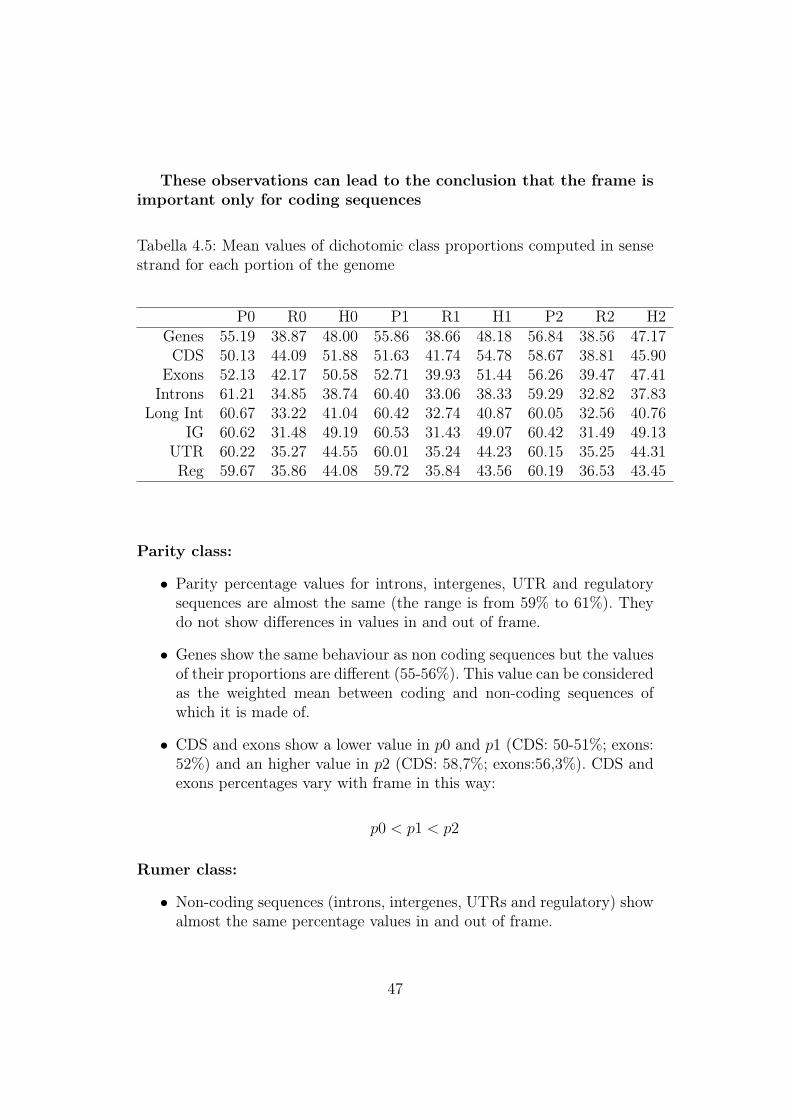
These observations can lead to the conclusion that the frame isimportant only for coding sequences

Tabella 4.5: Mean values of dichotomic class proportions computed in sensestrand for each portion of the genome

P0 R0 H0 P1 R1 H1 P2 R2 H2Genes 55.19 38.87 48.00 55.86 38.66 48.18 56.84 38.56 47.17CDS 50.13 44.09 51.88 51.63 41.74 54.78 58.67 38.81 45.90

Exons 52.13 42.17 50.58 52.71 39.93 51.44 56.26 39.47 47.41Introns 61.21 34.85 38.74 60.40 33.06 38.33 59.29 32.82 37.83

Long Int 60.67 33.22 41.04 60.42 32.74 40.87 60.05 32.56 40.76IG 60.62 31.48 49.19 60.53 31.43 49.07 60.42 31.49 49.13

UTR 60.22 35.27 44.55 60.01 35.24 44.23 60.15 35.25 44.31Reg 59.67 35.86 44.08 59.72 35.84 43.56 60.19 36.53 43.45

Parity class:

• Parity percentage values for introns, intergenes, UTR and regulatorysequences are almost the same (the range is from 59% to 61%). Theydo not show differences in values in and out of frame.

• Genes show the same behaviour as non coding sequences but the valuesof their proportions are different (55-56%). This value can be consideredas the weighted mean between coding and non-coding sequences ofwhich it is made of.

• CDS and exons show a lower value in p0 and p1 (CDS: 50-51%; exons:52%) and an higher value in p2 (CDS: 58,7%; exons:56,3%). CDS andexons percentages vary with frame in this way:

p0 < p1 < p2

Rumer class:

• Non-coding sequences (introns, intergenes, UTRs and regulatory) showalmost the same percentage values in and out of frame.

47

• UTR and regulatory sequences show values between 35% and 36%,while introns percentages vary within 32,8% and 34,8%.

• Intergenes seems to have a specific Rumer percentage value that isaround 31%

• Genes show the same behaviour as non coding sequences but the valuesof their percentages are around 39%). This value can be consideredagain as the weighted mean between coding and non-coding sequencesof which it is made of.

• Coding sequences proportions vary with the frame in this way:

r2 < r1 < r0

Their values are remarkably higher than non-coding ones, in particularfor what concerns r0 (CDS: 44%, exons: 42%).

Hidden class

• Non-coding sequences (introns, intergenes, UTRs and regulatory) showalmost the same percentage values in and out of frame but with specificvalues for each sequence class: introns (38%) , intergenes (49,1%), UTRsand regulatory(44%)

• Once again coding sequences show a different pattern that take intoaccount the frame:

h2 < h0 < h1

For what concerns exons, we can see again that h0 is very similar toh1 (50,6% and 51,4%) but higher than h2 (47,4%)

• Once again genes show the same behaviour as non coding sequences(they do not change with frame) but the values of their percentages(about 48%) can be considered as the weighted mean between codingand non-coding sequences of which it is made of.

• Finally it is interesting to underline that introns seem to minimizehidden class.

48

Antisense strand

Analyzing dichotomic classes percentages in antisense strand (see Table 4.2.1),we can observe a similar behaviour for coding and non-coding sequences withrespect to what is described in sense strand:

• Genes and non coding sequences do not seem to consider frame, whileexons and CDS do.

• Percentage values are different from the ones observed in sense strand.This is valid for all the sequence classes except intergenes.

Surprisingly, intergenes show the same percentage values thatwe observed analysing sense strand

• For the other non-coding sequences (introns, long introns, UTR andregulatory) we can see that parity percentage values are similar tothose computed in sense strand, while Rumer and hidden percentagevalues differ from sense strand ones.

• CDS and exons show again a frame-related behaviour:

p2a < p0a < p1a

r0a < r2a < r1a

h2a < h0a < h1a

Tabella 4.6: Mean values of dichotomic class proportions computed inantisense strand for each portion of the genome

P0a R0a H0a P1a R1a H1a P2a R2a H2aGenes 56.29 38.60 51.04 56.33 39.33 51.01 56.01 39.09 50.59CDS 54.61 39.05 48.66 56.33 49.32 49.39 51.06 43.64 44.14

Exons 54.85 40.75 49.09 55.92 45.28 49.27 53.29 42.76 47.06Introns 60.45 29.38 61.01 61.58 26.75 61.68 61.74 28.64 61.36

Long Int 60.57 29.15 58.66 60.92 28.43 58.85 60.94 29.04 58.78IG 60.56 31.56 49.12 60.47 31.56 49.09 60.54 31.53 49.14

UTR 60.12 32.16 52.20 59.70 32.40 52.30 59.71 32.19 52.65Reg 60.39 32.61 49.50 59.74 33.28 48.97 59.18 33.15 49.13

49

4.2.2 Complementary sequences

Complementary sequences are those sequences which undergo to strong/weakglobal transformation that is A is converted to T while C is converted to G(and viceversa). We applied this transformation to all the sequences consi-dered before and then we computed dichotomic classes proportions again onsense and antisense strand (the relative tables are shown in Appendix A).

Sense strand

Also in complementary sequences we can see that coding and non-codingsequences show the different behaviour observed in normal sequences: in factonly exons and CDS show different mean and median values in differentframes.

Proportions values for introns, long introns, intergenes, UTRs and regu-latory sequences are almost the same in and out of frame for each dichotomicclass.

Genes show the same behaviour as non coding sequences but the values oftheir proportions are different. This value can be considered as the weightedmean between coding and non-coding sequences of which it is made of.

CDS and exons proportions vary with frame in this way:

p0 < p2 < p1

r1 < r0 < r2

h1 < h0 < h2

Finally we can observe that proportion values are different from the onecomputed in normal sequences for all classes except for intergenes.

Antisense strand

We can make the same considerations as in sense strand. The only differenceis the proportions pattern of CDS and exons:

p0a < p1a < p2a

r1a < r0a < r2a

h1a < h0a < h2a

We have to underline that proportions in intergenes sequences are exactlythe same as in sense strand and in sense and antisense strand of normalsequence!!

50

p = 60%, r = 31%, h = 50%

4.2.3 Reverted sequences

Computing dichotomic classes on a reverted sequence is like computing di-chotomic class on the antisense strand of the complementary sequence. The-refore in this section we have a copy of the tables shown in the previous one(i.e: complementary sense strand is identical to reverted antisense strand andviceversa).

4.2.4 Keto/Amino global transformation sequences

Sequences that undergo to keto/amino global transformation convert A to Cand G to C (and viceversa). We applied this transformation to all the normalsequences and then we computed dichotomic classes percentages again onsense and antisense strand (the relative tables are shown in Appendix A).

Sense strand

Also in this case we can see that only exons and CDS show different meanand median values in different frames.

Proportions values for introns, long introns, intergenes, UTRs and regu-latory sequences are almost the same in and out of frame for each dichotomicclass. In particular, percentages of UTRs and regulatory sequences are almostthe same between them

Genes show the same behaviour as non coding sequences but the values oftheir percentages are different. This value can be considered as the weightedmean between coding and non-coding sequences of which it is made of.

CDS and exons percentages vary with frame in this way:

p0 < p2 < p1

r0 < r1 < r2

h0 < h1 < h2

Finally we can observe that percentage values are different from theone computed in normal and complementary sequences for all classes (alsointergenes).

51

Antisense strand

We can make the same considerations as in sense strand. The only differenceis the percentages pattern of CDS and exons:

p2a < p1a < p0a

r1a < r2a < r0a

h1a < h2a < h0a

Moreover, we can notice that intergenes percentages are the same com-puted in sense strand.

4.2.5 Purine/Pyrimidine global transformation sequen-ces

Sequences that undergo to purine/pyrimidine global transformation convertA to G and C to T (and viceversa). We applied this transformation to allthe normal sequences and then we computed dichotomic classes percenta-ges again on sense and antisense strand (the relative tables are shown inAppendix A).

Sense strand

We can make the same general considerations done for keto/amino globaltransformation.

CDS and exons proportions vary with frame in this way:

p2 < p1 < p0

r2 < r0 < r1

h2 < h1 < h0

It is important to underline that percentages of intergenes are the sameobserved in sense and antisense strand of keto/amino global transformationsequences.

Antisense strand

The proportions pattern of CDS and exons is:

p1a < p0a < p2a

r2a < r0a < r1a

52

h0a < h2a < h1a

As expected the percentages pattern of intergenes is the same as in sensestrand!!

p = 40%, r = 67%, h = 50%

4.2.6 Comments

By these observations we could speculate that:

• Since dichotomic classes percentages vary with frame only for codingsequences, the frame is important only for coding sequences and dicho-tomic calsses can be useful to recognize it.

• All dichotomic classes can distinguish between coding and non-codingsequences, in fact their percentage values are always different. In par-ticular, if we consider, for example, normal sequences we can see that:

– Parity could discriminate also between sense and antisense codingsequences. In fact it is always around 60% for non-coding sequen-ces (in both strands), while it is remarkably lower for CDS andexons and, moreover, it varies with strand: p0 in sense strand seemto be a bit lower (50-52%) than in antisense strand (54%). Similardifferences can be found for p1 and p2.

– Since Rumer and hidden percentage values vary between non-coding sequences and, moreover, between sense and antisense strand,they are useful to discriminate between the different classes of non-coding sequences (i.e: introns, long introns, intergenes, UTRs andregulatory)

Similar considerations can be done for complementary, reverted, ke-to/amino and purine/pyrimidine transformated sequences.

• Since intergenes sequences show the same pattern of dichotomic classespercentages in sense and antisense strand, they could be consideredas the expression of a random sequence (they don’t carry any kind ofinformation)

• Finally, for what concerns coding sequences, we can see that CDS showproportions values that differ with frame a bit more than exons ones.For example, if we consider parity, we can see that:

53

– p0 and p1 values are almost the same for exons (p0 = 52, 1%,p1 = 52, 7%) while they differ a bit more for CDS (p0 = 50, 1, p1 =51, 6)

– p2 value is higher for CDS than for exons (58,7% and 56,3%respectively)

This kind of difference can be observed in Rumer and hidden propor-tions too. This could suggest that there is a sort of “union effect” thatoccurs when fragments of coding sequences (exons) join together toform a CDS.

4.3 Independence testNow I want to check if the information provided by these properties is spe-cific for dichotomic classes or simply comes from the proportion of bases inthe original sequence. In the latter case, the information content should bealways the same, regardless of the order of bases within the sequence if theirproportions are kept constant. If, given a nucleotide sequence A, I perform apermutation of the basis without changing their number, I get a new sequen-ce B with the same proportion of the four bases (A,C,G,T). However, thedichotomic classes binary strings computed from the two original sequences(A and B) will be different (for what concerns parity class we will get PA andPB. If the proportion of 1 in each binary string (PA and PB) is the same, thenthe information carried by dichotomic classes depends only on the proportionof bases. Otherwise we can state that dichotomic classes carry an additionalinformation content, with respect to that carried by the proportion of basesin the original sequence.

For instance, define the random variable X as the parity of a dinucleotidefor a given sequence. Then,X follows a Bernoulli distribution with parameterπ = P (X = 1), that is: E(X) = π and V (X) = π(1− π). Then, we have thefollowing null hypothesis:

H0 : π = π0

H1 : π 6= π0

where π0 = P (X = 1) under the assumption that the DNA sequence is anexpression af an i.i.d. process, that is its sequence is randomly derived on thebasis of a given proportion of the four bases. Now, we can see that:

54

π0 = P (X = 1) = P (D) ∈ S1 =8∑i=1

P (b1)i ∗ P (b2)i (4.1)

where:

• D is the dinucleotide considered

• S1 and S0 are, respectively the group of dinucleotides that correspondto parity class 1 (S1) and parity class 0 (S0)

• b1 and b2 are, respectively, the bases in the first and in the secondposition of the dinucleotide.

• P (b1) and P (b2) are the probability of occurrences of the 4 nucleotides(T,C,A,G) in the first and second base, respectively.

The association scheme for the parity is presented in Table 4.7. Therefore,the possible differences observed between the original and i.i.d. sequences arenot due to the proportion of bases and all the quantities derived from it (e.g.the GC content and the like).For example, if we have the following probability distribution for the nucleo-tides: 1

base PA 0.20C 0.25G 0.20T 0.35

then

π0 = 0.20× 0.20 + 0.25× 0.20 + 0.20× 0.20 + 0.35× 0.20 + 0.20× 0.35+

+ 0.35× 0.35 + 0.20× 0.25 + 0.35× 0.25 = 0.53

Now, if we take the usual sample mean π̂ as the estimator of π we have thatunder the null hypothesis, E(π̂) = π0 and V (π̂) = π0(1−π0)

nwhere n is the

length of binary sequence. Thus, we can use the test statistic Z

Z =π̂ − π0√π0(1−π0)

n

.

1They are global (not position-dependent) proportions

55

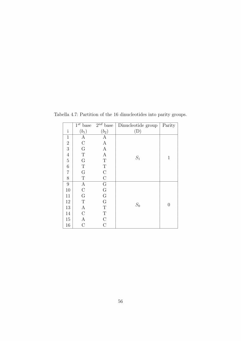
Tabella 4.7: Partition of the 16 dinucleotides into parity groups.

1st base 2nd base Dinucleotide group Parityi (b1) (b2) (D)1 A A

S1 1

2 C A3 G A4 T A5 G T6 T T7 G C8 T C9 A G

S0 0

10 C G11 G G12 T G13 A T14 C T15 A C16 C C

56

Z converges in distribution to a standard normal random variable so thatthe usual critical values can be used.

I have computed the p-values associated to the test for each sequence andfor each dichotomic class. The results are shown in Figures 4.3 and 4.4, wherewe present the histograms of the p-values for the sequences analyzed.

Tabella 4.8: Percentages of p-values lower than 0.05

Parity Rumer HiddenGenes 17.94 13.24 8.93CDS 28.28 14.96 5.80

Exons 11.45 5.80 4.00Introns 4.31 1.50 1.20

Long introns 5.71 1.84 1.43Intergenes 9.09 3.13 1.70

UTR 6.27 1.98 1.43Regulatory 5.65 2.85 1.96

4.3.1 Comments

By looking at the histograms in Figures 4.3 and 4.4, we can see that:

• only coding sequences and genes show a pattern which indicates thepresence of differences between the proportions values computed onoriginal sequences and those computed on sequences whose propertiesbelongs only to proportions of bases. Only these classes, in fact, show animportant rate of p-value lower than 0.05. That could mean that onlygenes, exons and CDS are non-random sequences with an informativecontent.

• parity sequences seem to be more informative. They show, in fact, an hi-gher rate of low p-values. This trend can be observed also in non-codingsequences where parity p-values seem to follow an uniform distributionwhile Rumer and hidden show fewer low p-values.

• If we compare graphs relative to exons and CDS we can see that thelatter show an higher rate of low p-values. This effect could be relatedto the sample size. However, this observation could be also a furtherindication of the presence of a “union effect” that occurs when fragmentsof coding sequences (exons) join together to form a CDS.

57

Figura 4.3: Histograms of the p-values associated to the independence testfor genes, intergenes, exons and CDS

58

Figura 4.4: Histograms of the p-values associated to the independence testfor introns,long introns, UTRs and regulatory sequences

59

The latter issue might be also studied by resorting to adjusted p-valuesand to false discovery rate estimation (see e.g. [11]). The overall resultsconfirm the findings of [20] regarding the presence of correlations betweendichotomic classes in coding sequences.

4.4 ConclusionsThe analysis of bases distributions and percentage of dichotomic classes di-stributions is helpful in order to characterize different portions of the genomein A.thaliana chromosome 1 and it leads to the following considerations:

• Coding and non-coding sequences show different patterns of distribu-tion. Since the percentages of dichotomic classes vary with frame onlyfor coding sequences, we can conjecture that frame is important onlyfor these kind of sequences (CDS and exons).

• Dichotomic classes seem to be useful in order to recognize coding se-quences. In fact all the dichotomic classes can distinguish between co-ding and non-coding sequences: their mean values are always different.

• Parity class could discriminate also between sense and antisense codingsequences: while the mean percentage for non-coding sequences is al-ways around 60% (in both strands), it is remarkably lower and stranddependent for CDS and exons.

• Rumer and hidden percentages vary in both strand between coding andnon-coding sequences. Therefore they are useful in order to discrimina-te between the different groups of non-coding sequences (i.e: introns,long introns, intergenes, UTR and regulatory sequences). In particular,introns seem to minimize hidden class.

• Intergenes show a constant distribution pattern that vary neither withframe nor with strand. They always show:

p ' 60%, r ' 31%, h ' 49%

• Finally, we can identify a sort of “union effect” that occurs when shortfragments of coding sequences (exons) join together to form a CDS. Infact mean percentage values of CDS in each dichotomic class differ varywith frame more than those of exons. For example, if we consider parity,we can see that p0 and p1 are almost the same for exons (p0=52.1%,p1=52.7%) while for CDS we have p0 = 50.1%, p1 = 51.6%. Moreover

60

the mean for p2 is higher for CDS than for exons (58.7% and 56.3%respectively). This kind of difference can be observed in Rumer andhidden percentages too.

• The results obtained from the independence tests show that the fra-mework suggested by dichotomic classes is able to uncover the existen-ce of significant correlations in those sequences that are involved inprotein synthesis.

61

Capitolo 5

Discriminating different portionsof the genome

In the previous chapter I showed how dichotomic classes can characterize thedifferent portions of A.thaliana genome. It means they may carry a quantityof information higher than that explained by the proportion of bases. The-refore, I want to answer the following question: is the information carriedby dichotomic classes useful in order to discriminate between two differentportions of the genome?

5.1 Classification through Logistic RegressionI try to answer this question with the help of logistic regression models thatis part of generalized linear models. Logistic regression allows to predict adiscrete outcome, such as group membership, from a set of variables that maybe continuous, discrete, dichotomous, or a mix of any of these. ([32] [28])

An explanation of logistic regression begins with an explanation of thelogistic function, which, like probabilities, always takes on values betweenzero and one:

π(x) =e(β0+β1x1)

e(β0+β1x1) + 1=

1

e−(β0+β1x1) + 1

The dependent variable in logistic regression is usually dichotomous, thatis, the dependent variable can take the value 1 with a probability of successπ, or the value 0 with probability of failure (1− π). This type of variable iscalled a Bernoulli (or binary) variable where:

Y ∼ Ber(π) E(Y ) = π V (Y ) = π(1− π)

62

As mentioned previously, the independent or predictor variables, in lo-gistic regression, can take any form, that is, logistic regression makes noassumption about the distribution of the independent variables. They do nothave to be normally distributed, linearly related or of equal variance withineach group. The relationship between the predictor and the response varia-bles is not a linear function in logistic regression. It is used a link function,called “logit transformation of π”:

π =eβ0+β1x1+β2x2+...+βkxk

1 + eβ0+β1x1+β2x2+...+βkxk

logit[π] = log

[π

1− π

]= β0 + β1x1 + β2x2 + ...+ βkxk

The goal of logistic regression is to correctly predict the category of out-come for individual cases using the most parsimonious model. To accomplishthis goal, a model is created that includes all predictor variables that areuseful in predicting the response variable.

The logistic regression method is used for example to make a classifica-tion. The response variable Y can assume two values that, for expositoryconvenience, we could call A and B. Let’s suppose that a certain observationbelongs to class A with probability π.

Starting from a set of data, namely a set of observations that are known,the coefficients of the model are calculated. Then, examining new observa-tions that we want to classify on the basis of mere knowledge of the predictors,we calculate the value of π and assign the observation to the class A if theprobability π exceeds a certain threshold (s).

Classification Classification models are tested by comparing the predictedvalues to known target values in a set of test data. The test data must becompatible with the data used to build the model and must be prepared inthe same way that the build data was prepared. Typically the build dataand test data come from the same historical data set. A percentage of therecords is used to build the model; the remaining records are used to test themodel.Test metrics are used to assess how accurately the model predicts theknown values. If the model performs well, it can then be applied to new datato predict the future.

In order to assess the prediction ability of the model it is useful to builda confusion matrix that displays the number of correct and incorrect predic-tions made by the model compared with the actual classifications in the testdata. The matrix is n× n, where n is the number of classes.

63

The following table shows a confusion matrix for a binary classificationmodel. The rows present the number of predicted classifications in the testdata. The columns present the number of observed classifications made bythe model.

observed0 1

predicted 0 n00 n01 n0·1 n10 n11 n1·

n·0 n·1 N

where N = n00 + n01 + n10 + n11 is the sample size of the test set.

W =n10 + n01

N100

I will use W , as the misclassification rate.

64

5.2 Sequence classification of A.thaliana chro-mosome 1

Sequence prediction can be seen as a classification problem:

Y = f(X1, ..., Xp) + ε

where Y is a dichotomic response variable and (X1, ..., Xp) is a set ofpredictors.

I would like to predict if a given sequence belongs (Y = 1) or not (Y = 0)to a specific portion of the genome (i.g: exons, introns, etc.) using dichotomicclasses percentages as predictors.

• Y ∼ Ber(π);

g (E[Y |X]) = β0 +

p∑i=1

βiXi . (5.1)

where g(π) = log π1−π is the link function.

I create logistic regression model in order to verify if some combination ofthe variables in the datasets can discriminate the different sequence classes.I take into account the following pairwise comparisons:

1. Exons vs Introns

2. CDS vs Long Introns

3. Exons vs CDS

4. Genes vs intergenes

5. Exons vs UTR

6. Introns vs UTRs

For each of these couple I created six logistic regression models that differsin number and kind of explanatory variables considered, as shown in Table5.1 and 5.2.

For each model I joined the two classes dataset. Then I divided the recordsinto two random groups: the first, containing 80% of records, is used to fitthe model, while the other (containing the remaining 20% of records) isused to make predictions and build the misclassification table (out of sampleanalysis).

65

Tabella 5.1: Logistic regression models created for each couple of sequenceclasses

Model RegressorsP p0, p1, p2R r0, r1, r2H h0, h1, h2Sen h0, h1, h2, p0, p1, p2, r0, r1, r2Anti h0a, h1a, h2a, p0a, p1a, p2a, r0a, r1a, r2aTot h0, h1, h2, p0, p1, p2, r0, r1, r2, h0a, h1a, h2a,

p0a, p1a, p2a, r0a, r1a, r2aB A, C, G, T

Tabella 5.2: Variables included in each dataset

Name Description

p0, r0, h0 mean value for parity, Rumer, hidden classes, inframe



p0a, r0a, h0a mean value for parity, Rumer, hidden classes,antisense strand in frame



66

5.2.1 Exons vs Introns

First, I want to assess if I can discriminate between intron and exons using,as regressors, the sets of variable defined in Table 5.1. I proceeded as follows:

• I create a dataset with both the sequences Then I define a new binaryvariable (named ”class”) that takes value 1 if the sequence is an intronand 0 if the sequence is an exon.

• I randomly divided th 68212 records into two groups:

– The first group composed by 53212 sequences was used in orderto build a logistic regression model

– The second group composed by 15000 sequences was used for outof sample analysis:

∗ I compute the estimation of π∗ I set a threshold value (s = 0.5)∗ If π > s then I consider the sequence as an intron, otherwise

I consider it as an exon.∗ Finally I build the confusion matrix and compute the misclas-

sification rate.

• I repeated this scheme for all the seven models defined in Table 5.1 andobtained the results as shown in Table 5.3 and Figure 5.1

Tabella 5.3: Misclassification rate for each model comparing exons and introns

Model Misclassificationrate (%)

P 15.72R 29.34H 21.39Sen 8.53Anti 7.17Tot 5.7B 5.81

We can see that:

67

• Models Sen, Anti, Tot and B discriminate with a good accuracy betweenintron and exon sequences. We can see that each of these model showa misclassification rate lower than 10%. The best models are tot and Bwith an error rate around 5.75%

• P, H and R models show higher misclassification rates. However parityclass percentages seem to discriminate better between intron and exonsequences than other dichotomic classes

68

Figura 5.1: Sequence prediction: introns vs. exons

69

5.2.2 CDS vs. Long introns

I randomly divided the 14794 records into two groups and used 3000 sequen-ces for out of sample analysis. The results are summarized in Table 5.4 andFigure 5.2.

Tabella 5.4: Misclassification rate for each model comparing CDS and longintron sequences


P 3.9R 12.37H 7.63Sen 1.93Anti 1.33Tot 1.27B 1.77

• All the models can discriminate with a good accuracy between the twogroups of sequences. The worst model is R-model, with a misclassifi-cation rate equal to 12.37%. All the other models show a rate of errorlower than 10%.

• In particular sen, anti, tot and B models discriminate with an excellentaccuracy (lower than 2%). The best model is tot (m.r.=1.27%).

Once again we can see that comparison between CDS and long intronspresents enhances the features observed in the comparison between exonsand introns.

70

Figura 5.2: Sequence prediction: CDS vs. long introns

71

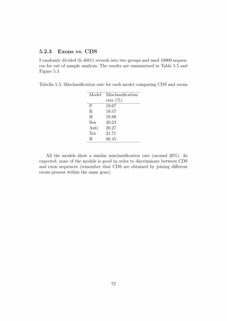
5.2.3 Exons vs. CDS

I randomly divided th 46811 records into two groups and used 10000 sequen-ces for out of sample analysis. The results are summarized in Table 5.5 andFigure 5.3

Tabella 5.5: Misclassification rate for each model comparing CDS and exons


P 19.67R 19.57H 19.89Sen 20.23Anti 20.27Tot 21.71B 80.45

All the models show a similar misclassification rate (around 20%). Asexpected, none of the models is good in order to discriminate between CDSand exon sequences (remember that CDS are obtained by joining differentexons present within the same gene).

72

Figura 5.3: Sequence prediction: exons vs. CDS

73

5.2.4 Genes vs. Intergenes

I randomly divided th 16778 records into two groups and used 3000 sequencesfor out of sample analysis. The results are summarized in Table 5.6 and Figure5.4

Tabella 5.6: Misclassification rate for each model comparing genes andinergenes


P 15.27R 19.4H 39.47Sen 15Anti 14.43Tot 14.2B 13.23

The misclassification rates in these model are quite high, in fact theyvary from 13,23% (B-model) to 19,4% (R-model). It is interesting to noticethat H-model is very bad, in fact it shows a really high misclassification rate(39,47%)

74

Figura 5.4: Sequence prediction: Genes vs. Intergenes

75

5.2.5 Exons vs. UTRs

I randomly divided the 51976 records into two groups and used 10000 se-quences for out of sample analysis. The results are summarized in Table 5.7and Figure 5.5

Tabella 5.7: Misclassification rate for each model comparing exons and UTRs


P 14.98R 25.8H 27.16Sen 12.6Anti 13.63Tot 11.9B 10.66

Misclassification rates vary from 10% to 15% except for R and H-modelsthat high shows misclassification rates (25,8 and 27,16% respectively). Oneagain parity class percentages seem to be better than Rumer and hidden’sones when coding sequences (exon and CDS) are involved.

76

Figura 5.5: Sequence prediction: exons vs. UTRs

77

5.2.6 Introns vs. UTRs

I randomly divided the 45090 records into two groups and used 10000 se-quences for out of sample analysis. The results are summarized in Table 5.8and Figure 5.6

Tabella 5.8: Misclassification rate for each model comparing UTR and Intronsequences


P 31.78R 31.27H 28.62Sen 26.09Anti 24.05Tot 20.2B 26.67

In these models misclassification rates are very high, varying from 20,2% (Tot-model) to 31,78 (P-model). It is interesting to underline that, in thiscase, H-model is better than P and R ones. In fact it happens every timeintrons are considered.

78

Figura 5.6: Sequence prediction: introns vs. UTRs

79

5.3 Comments• Models involving exons and CDS (sequences within a gene that are

transcripted and translated) show an good discrimination rate. In fact,it is possible to discriminate with a good sensitivity exons from intronsand, overall, CDS from Long introns.

– This could mean that A.thaliana cell has to distinguish betweencoding and non coding region within a DNA sequence. The di-scrimination power grows when we consider CDS instead of exonsindicating, as we have already seen before, a sort of “joined effect”occuring when different exons join to form a CDS

– It is evident how the percentage of bases is, itself, sufficient inorder to achieve the best discrimination rate.

∗ The only exception is the Tot-model that uses as regressorsall the percentages of dichotomic classes computed both insense and antisense strand.∗ Anyway, the gain of sensitivity is not so much to overcome

the parsimony of the B-model (3 vs. 18 regressors)

• P-models are usually better than R and H-models. This could meanthat parity class could discriminate better between the different por-tions of a gene.

• H-model (usually better than R-model) applied in order to discrimina-te between genes and intergenes seems to be very unhelpful. On thecontrary it is more sensitive in discriminating between CDS and longintrons. This could mean that hidden class represent a mathemati-cal structure meaningful only to recognize different portions of codingsequences

• Because the model B is almost always the best model, the computationof dichotomic classes seems not to be useful for the discrimination bet-ween the different portions of the genome, since it seems to be sufficientthe computation of the proportion of bases.

80

Capitolo 6

Dependence analysis

The analysis conducted in the previous chapter showed that the dichoto-mic classes carry no informational advantage for classification purposes ifcompared to proportions of bases. However, the information content of thedichotomic classes could detect the presence of short-range dependence struc-tures within genome sequences. Therefore, in this chapter, I want to check ifthere is any dependence structure in the dichotomic classes within differentportions of a gene.

In information theory and coding theory with applications in computerscience and telecommunication, error detection and correction or error con-trol are techniques that enable reliable delivery of digital data over unreliablecommunication channels. Many communication channels are subject to chan-nel noise, and thus errors may be introduced during transmission from thesource to a receiver. Error detection techniques allow detecting such errors,while error correction enables reconstruction of the original data.

The general idea for achieving error detection and correction is to addsome redundancy (i.e., some extra data) to a message, which receivers canuse to check consistency of the delivered message, and to recover data deter-mined to be corrupted. Error-detection and correction schemes can be eithersystematic or non-systematic: In a systematic scheme, the transmitter sendsthe original data, and attaches a fixed number of check bits (or parity data),which are derived from the data bits by some deterministic algorithm. If onlyerror detection is required, a receiver can simply apply the same algorithmto the received data bits and compare its output with the received checkbits; if the values do not match, an error has occurred at some point duringthe transmission. In a system that uses a non-systematic code, the originalmessage is transformed into an encoded message that has at least as manybits as the original message.

Redundancy and degeneracy are two main features of a communication

81

code with an error detection and correction system. Since the genetic codeis redundant and degenerate it is supposed to have such a system: it is astill open challenge linking information theory and biology. Moreover it isknown that DNA-polymerase shows a proofreading ability in order to detectand correct some point mutations during DNA-replication process. Whenan error is detected, these polymerases halt the process of DNA replication,work backward to remove nucleotides from the daughter DNA chain untilit is apparent that the improper nucleotide is gone, and then reinitiate theforward replication process.

The existence of a coding mechanism for error correction/detection im-plies some kind of dependence inside data and several studies have highlightedthe presence of fractal long-range correlations in nucleotide sequences. Howe-ver, error detection and correction should act at a local level. The existenceof a dependence structure in the dichotomic classes has been demonstrated[19, 20].

The objective of my analysis is to assess if there is a dependence structurein the genome sequence of A.thaliana and if it is present within all the dif-ferent portions of the genome. Moreover I would like to assess if dichotomicclasses can detect such dependence structure.

In order to try to answer this question I will perform the same analysis asin [19, 20] applied to different portions of the genome.

6.1 Dependence measuresIn statistics, dependence refers to any statistical relationship between two ormore random variables. Formally, dependence refers to any situation in whichrandom variables do not satisfy a mathematical condition of probabilisticindependence:

Two events A and B are independent if and only if their joint probabilityequals the product of their probabilities:

P (A ∩B) = P (A)P (B)

Similarly, Two random variables X and Y are independent if and only iffor every a and b, the events {X ≤ a} and {Y ≤ b} are independent events(as defined above). That is, X and Y with cumulative distribution functionsFX(x) and FY (y), and probability densities fX(x) and fY (y), are independentif and only if the joint random variable (X,Y) has a cumulative distributionfunction

82

FX,Y (x, y) = FX(x)FY (y),

or equivalently, a joint density

fX,Y (x, y) = fX(x)fY (y).

There is an extensive literature on how to measure dependence, mainly onthe basis of the distance between the joint distribution of the data and theproduct of the marginal distributions, where the latter distribution assumesthe property of independence. [30, 2, 52, 37, 46, 25, 13].

The most commonly used measures of dependence and test statistics be-longs to ”correlation” function. This is motivated by linear relations involvingcontinuous variables and/or Gaussian processes. These measures tend to failwhen variables are discrete, or in detection, as when they face nonlinear, ornon-Gaussian processes. The currently dominant measures tend to be func-tions of only one or two moments of the underlying processes. While this hasthe advantage of simplicity, it can mislead when distinctions between the tailareas and higher order moments are germane. Thus, it is clearly desirable formeasures of association and dependence to be robust towards possible (butunknown) nonlinearities and non-Gaussian processes.

In recent years there have been developed several different methods andindicators statistics of dependence, using the concepts of entropy borrowedfrom information theory. Some of them are finalized to measure the level ofdependence, autocorrelation and irregularities of the fluctuations of a sin-gle series or of multiple series between them (dependence,correlation andsynchronization).

Examples of other “well-informed” measures include the moment genera-ting and characteristic functions, as well as many entropy functionals deve-loped in information theory. Entropies are defined over the space of distri-butions which form the bases of independence/dependence concepts in bothcontinuous and discrete cases. Entropy is also dimensionless as it appliesseamlessly to univariate and multivariate contexts.

In information theory, entropy is a measure of the uncertainty associatedwith a random variable [34]. In this context, the term usually refers to theShannon entropy, which quantifies the expected value of the informationcontained in a message. Equivalently, the Shannon entropy is a measure ofthe average information content one is missing when one does not know thevalue of the random variable. The concept was introduced by Claude E.Shannon in his 1948 paper “A Mathematical Theory of Communication” [47].The Shannon entropy of a random variable (r.v) X is defined as:

83

H(X) = −n∑i=1

pi log2 pi

In this chapter consider three measures of dependence

• Chi-squared test

• Sρ (a normalized variant of the Bhattacharya-Hellinger-Matusita di-stance)

• Average mutual information

6.1.1 Chi-squared test for independence

Chi-squared test allows us to study the relationship between two categoricalvariables. In particular, the chi-square test is used to test the null hypothesisthat the variables, indicated with X and Y are independent.

Given the double random variable (X, Y), consider the following jointprobability distribution:

y1 · · · yk · · · ycx1 π11 · · · π1k · · · π1c π10...

... . . . ... . . . ......

xj πj1 · · · πjk · · · πjc πj0...

... . . . ... . . . ......

xr πr1 · · · πrk · · · πrc πr0π01 · · · π0k · · · π0c 1

where:

• x1, x2, ..., xj, ..., xr and y1, y2, ..., yk, ..., yc, are, respectively, the possiblerealizations of X and Y;

• πjk is the joint probability that the v.a. X takes the value xj and v.a.Y takes the value yk:

πjk = P (X = xj, Y = yk), j = 1, ..., r, k = 1, ..., c;

84

• πj0 is the marginal probability that the v.a. X takes the value xj (forany value of Y), or

πj0 = P (X = xj) =c∑

k=1

πjk j = 1, ..., r;

• π0k is the marginal probability that the v.a. Y takes the value yk ((forany value of X), or

π0k = P (Y = yk) =r∑j=1

πjk k = 1, ..., c.

The null hypothesis is that X and Y are independent, namely:

P (X = xj, Y = yk) = P (X = xj)P (Y = yk)

or, equivalently, that:

πjk = πj0 · π0kwith j = 1, ..., r k = 1, ..., c.Therefore, the problem can be formalized as follows:

H0 : ∀j, k πjk = πj0 · π0k,

H1 : ∀j, k πjk 6= πj0 · π0k.

Given a random sample from a. double v.a (X, Y), consider the followingcontingency Table (r × c):

y1 · · · yk · · · ycx1 n11 · · · n1k · · · n1c n10...

... . . . ... . . . ......

xj nj1 · · · njk · · · njc nj0...

... . . . ... . . . ......

xr nr1 · · · nrk · · · nrc nr0n01 · · · n0k · · · n0c n

where :

• x1, x2, ..., xj, ..., xr and y1, y2, ..., yk, ..., yc, are, respectively, the possiblerealizations of X and Y;

85

• njk is the frequency with which it is presented in the sample pair(xj, yk);

• nj0 is the marginal frequency of the sample realization xj, for any valueof Y:

nj0 =c∑

k=1

njk j = 1, ..., r

• n0k is the marginal frequency of the sample realization yj, for any valueof X:

n0k =r∑j=1

njk k = 1, ..., c

The maximum likelihood estimators π̂jk, π̂j0, π̂0k for the probability πjk, πj0andπ0k, coincide with the corresponding sample relative frequency, as follows:

π̂jk =njkn

; π̂j0 =nj0n

; π̂0k =n0k

nMoreover, in case the hypothesis of independence between X and Y is

true, the following relationship is expected to hold:

π̂0jk = π̂j0 · π̂0k

or, multiplying both sides by n:

n0jk =

nj0 · n0k

n, j = 1, ..., r; k = 1, ..., c.

N.B. ”0” symbol in the apex means that we are considering H0 as trueTherefore, the test of independence between X and Y can be conducted

on the quantities:

(njk − n0jk)

2, j = 1, ..., r; k = 1, ..., c

that is, on the squared distances between the sampling frequency and thecorresponding expected frequencies in the case of independence.

If the differences between njk and n0jk are not too high, we will accept the

H0 hypothesis of independence between X and Y, otherwise we will have toreject it.. In particular, the test statistics is as follows:

Y0 =r∑j=1

c∑k=1

(njk − n0jk)

2

n0jk

,

86

with

n0jk =

nj0 · n0k

n

If H0 is true Y0 converges in distribution to a χ2 r.v. with (r − 1)(c− 1)degrees of freedom.

Y0 → χ2(r−1)(c−1)

Once the significance level of the test is fixed, we have the followingdecision rule:

A : Y0 < y(g;α), R : Y0 ≤ y(g;α),

where y(g;α) is the above centile of the χ2 distribution with g = (r−1)(c−1)d.f.

6.1.2 Mutual information

A second measure of dependence between two random variables X and Y isgiven by the mutual information [6]:

I(X, Y ) =∑i

∑j

p(xi, yj)log2p(xi, yj)

p(xi)p(yj)

If the two variables are independent, the mutual information betweenthem is zero. If the two are strongly dependent, e.g., one is a function ofanother, the mutual information between them is large. There are other in-terpretations of the mutual information; for example, the stored informationin one variable about another variable, and the degree of the predictabilityof the second variable by knowing the first. Clearly, all these interpretationsare related to the same notion of dependence and correlation [40].

The previous equation can be rewritten as follows:

87

I(X, Y ) =∑i

∑j

p(xi, yj)log2p(xi, yj)

p(xi)p(yj)

=∑i

∑j

p(xi, yj)log2p(xi, yj) +∑i

∑j

p(xi, yj)log21

p(xi)+

+∑i

∑j

p(xi, yj)log21

p(yj)+

=∑i

∑j

p(xi, yj)log2p(xi, yj)−∑i

p(xi)log2p(xi)−∑j

p(yj)log2p(yj)

= −H(X, Y ) +H(X) +H(Y )

ovvero

I(X, Y ) = H(X) +H(Y )−H(X, Y )

= H(X)−H(X|Y )

= H(Y )−H(Y |X)

Therefore, it is clear that the mutual information between two randomvariables is nothing more than the reduction of uncertainty of a variable dueto knowledge of the other. If the knowledge of Y reduces our uncertaintyabout X, then we say that Y carries information about X.

If X and Y are independently distributed, ie if p(x, y) = p(x)p(y),the mu-tual information between the two variables is zero. In addition, this measureis symmetric, that is

I(X, Y ) = I(Y,X)

and is always non-negative.Mutual information provides an indication of the link between two varia-

bles random X and Y. In particular it:

• assumes the value zero if only if p(x, y) = p(x)p(y), that is, if thevariables X and Y are independent;

• is always non-negative, then I(X, Y ) > 0;

• in the continuous case we have that I(X, Y ) = +∞ if Y = g(X) thatis the indicator tends to positive infinity if there is a perfect relation,although not linear, between X and Y.

88

Mutual information has been proposed, for example, as a criterion onwhich base test of independence and for the study of the level of dependency(not linear) in time series [10], [9].

In the present work I will compute mutual information between twodichotomic class sequences such that:

I(Xt, Yt+k) =∑i

∑j

p(xt, yt+k)log2p(xt, yt+k)

p(xt)p(yt+k)

where

• Xt(·) is a random process that measures which digit appears at positiont of the first dichotomic class sequence

• Yt+k(·) is a random process that measures which digit appears at posi-tion t+ k of the second dichotomic class sequence

• (Xt, Yt+k) is the bivariate random process that measures the joint ap-pearance of Xt(·) at position t and Yt+k(·) at position t+ k

6.1.3 Sρ

Shannon’s relative entropy and almost all other entropies fail to be “metrics”,as they violate either symmetry, or the triangularity rule, or both. This meansthat they are measures of divergence, not distance. A metric measure wouldhave the additional advantage of allowing multiple comparisons of depar-tures/distances. It is also desirable to provide the framework for assessingstatistical significance of any proposed measure. [49], [24]

Among the various indices based on the concept of entropy cited in theliterature, it is worth mentioning that proposed by Granger, Maasoumi andRacine [25], more often referred to as Sρ and defined as:

Sρ(k) =1

2

∫ +∞

−∞

∫ +∞

−∞

(f

12 − f

121 f

122

)2dxdy

where f is the joint density distribution of the random variables X andY, while f1 and f2 are their respective distributions of marginal densities.If X and Y are independent, Sρ = 0 otherwise, Sρ is positive and grea-ter than zero. Granger, Maasoumi Racine and developed the Sρ based onHellinger-Battacharya-Matusita distance measure [25] [41]. In particular, theBattacharya coefficient on the generic distributions fa and fb is defined as in[5] [1]:

89

ρ∗(fa, fb) =

∫ +∞

−∞(fafb)

12dx

and is a measure of divergence between distributions. This coefficientdoes not have a metrical structure because it does not meet all three axioms.On the contrary, its modified version is a metric distance, known as theBattacharya distance:

B(fa, fb) =√1− ρ∗(fa, fb)

Matusita measure, has the following form [47] [26]:

M(f − a, fb) =∫ +∞

−∞(f

12a − f

12b )

2dx

Between these two indicators there is the following relation:

M(fa, fb) = 2B(fa, fb)2

Both M(fa, fb) and B(fa, fb), a rare case between the measures of di-vergence, have the peculiar characteristic to meet, among other things, thetriangular inequality and therefore can be considered as metric measures

Moreover, if we replace fa with the joint density distribution of the ran-dom variables X and Y (f = f(X, Y )) and fb with the product of therespective marginal density distributions (f1f2) the we will obtain Sρ:

Sρ = 1− ρ∗(fa, fb) = B(fa, fb)2

Sρ is therefore a metric too and has a close relation with the Havrda andCharvat entropies family of k-order:

Ik(f1, f2) =1

k − 1

[∫(fk1 /f

k2 )dF2 − 1

], k 6= 1

Sρ is an indicator that can measure the degree of deviation from the con-dition of independence and is robust against possible (but unknown) nonli-near and non-Gaussian processes. In fact, the entropy of Granger, Maasoumiand Racine normalized to its maximum formally meets the following sixproperties:

1. It is well defined for both continuous and discrete variables.

2. It is normalized to zero if X and Y are independent, and lies between0 and +1.

90

3. The modulus of the measure is equal to unity (or a maximum) if there isa measurable exact (nonlinear) relationship, Y = m(X) say, betweenthe random variables.

4. It is equal to or has a simple relationship with the (linear) correlationcoefficient in the case of a bivariate normal distribution.

5. It is metric, i.e., it is a true measure of ”distance” and not just ofdivergence.

6. The measure is invariant under continuous and strictly increasing tran-sformations ψ(·). This is useful since X and Y are independent if andonly if ψ(X) and ψ(Y ) are independent. Invariance is important sinceotherwise clever or inadvertent transformations would produce differentlevels of dependence.

For a detailed discussion on the definition, implementation and estimationissues of Sρ, see [25].

In the present work, the statistical analysis of binary sequences obtained bymeans of our coding framework is based on the implementation of a bivariateversion of the metric entropy measure Sρ. This version corresponds to atwo-dimensional implementation of the methods employed in [19], as follows:

Sρ(k) =1

2

∫ ∫ [√f(Xt,Yt+k)(x, y)−

√fXt(x)fYt+k

(y)]2dxdy

where

• Xt(·) is a random process that measures which nucleotide appears atposition t

• (Xt, Yt+k) is the bivariate random process that measures the joint ap-pearance of Xt(·) at position t and Yt+k(·) at position t+ k

The measure has been proven to have impressive and robust power forcharacterizing nonlinear processes. In particular, it has been shown that testsbased upon Sρ have very good performances in terms of power and size [15].In the binary case the double integral reduces to summation and probabilitiesare estimated through relative frequencies:

Sρ(k) =1

2

1∑i=0

1∑j=0

[√Pr(Xt = i, Yt+k = j)−

√Pr(Xt = i)Pr(Yt+k = j)

]2

91

Tabella 6.1: Legend

class frame anticodonp = parity 0 = in frame a = reversed complementr = Rumer 1 = out of frame 1h = hidden 2 = out of frame 2

6.2 Sequence analysisIn previous works [19, 20] the authors analyzed both the univariate depen-dence structure of parity sequences generated from protein coding DNA re-gions, and bivariate dependence structure comparing pairwise chemical ordichotomic codon classes.

In this work, I would like to assess the short-range dependence stucturesbetween dichotomic classes computed on nucleotide sequences of differentportions of the genome. In order to do that, I have analyzed the followingset of sequences:

Group # of sequencesExons 500CDS 100

Introns 500Long introns 100Intergens 250UTR 100

For each sequence, I computed all the possible nontrivial combinationsof dichotomic classes (an overall set of 153 different cases): Then I compu-ted the dependence measure between the two binary strings relative to eachcombination at lag -1, 0 and +1.

Given two binary sequences Xt and Yt the null hypothesis tested is:{H0 : Xt and Yt+k are independentH1 : Xt and Yt+k are not independent

for k ∈ Z

and pXt(x) is the relative frequency of Xt;

pYt+k(y) is the relative frequencyYt+k;

p(Xt,Yt+k)(x, y) is the joint relative frequency (Xt, Yt+k).

92

In order to build a valid test, I need a suitable measure of dependence and ascheme for testing H0.

Measures I use the three dependence measures (D) described in the pre-viuos section:

1. Chi-squared test

2. Sρ (a normalized variant of the Bhattacharya-Hellinger-Matusita di-stance)

3. Mutual information

We must consider that:

• the null hypothesis we test is that of independence between binarysequences, that is, the absence of an informational organization betweencodons

• the dichotomic classes are naturally correlated because they can becomputed on the same bases

• spurious correlations due to nonstationarity/different GC content

• when comparing dichotomic classes the test does not have to depend oncorrelations induced by their definition; in fact, some specific combina-tions of dichotomic classes and reading frames induce nonzero spuriouscorrelations even in random sequences.

Because of such issues simple nonparametric bootstrap schemes that re-sample the binary sequences are not appropriate.

Testing scheme The above requirements can be satisfied by resortingto suitable nonparametric bootstrap or permutation schemes proposed in[19, 20]. The original DNA base sequence is randomly permuted. On thisnew sequence, the chemical (or dichotomic) classes are computed and thedependence measure D is estimated. The procedure is repeated B times (sayB=5000) as to obtain the bootstrap distribution of Sρ under the null hypo-thesis. Clearly, each permutation of the original data preserves the originalproportion of bases and this fulfils requirement.

93

Given a nucleotide sequence Zt

1. compute the two dichotomic classes Xt and Yt on Zt

2. compute the measure on Xt and Yt+k: D̂k

3. draw Z∗t , a random permutation of Zt

4. compute the two dichotomic classes X∗t and Y ∗t on Z∗t

5. compute the measure on X∗t and Y ∗t+k: D̂∗k

6. repeat steps 3 – 5 B times.

7. compare D̂k with the quantiles of the distribution of D̂∗k.

I applied the testing scheme to all the three dependence measures consi-dered.

94

6.2.1 Results

CDS

Looking at Table 6.2 we can see that:

• There is a strong dependence between dichotomic classes h0a and r1aat lag 0: in fact it is present in 60% of the sequences analyzed.

• Strong dependence seems to involve also:

– h1a and r2 at lag 0

– h0 and r2 at lag 0

– h2 and r1a at lag1

All of these couples of dichotomic classes are dependent in at least the40% of the sequences I analyzed. Table 6.2.1 display the differencesbetween CDS and the other portions of the genome: we can observe aclear prevalence of dependence structures in sequences CDS.

• As far as Sρ and mutual information (MI) concern, there are 10 coupleof dichotomic classes that show a dependence structure at least in 30 %of sequences. These structures involves only Rumer and hidden classes.

• Sρ and MI shows a very similar pattern. They seem to recognize thesame dependence structures with the same level of accuracy.

• χ2 − test recognize the same kind of dependence structure as Sρ andMI, but it shows a lower sensibility

Exons

We can see the same dependence structures observed for CDS sequences but,in this case, they are present in a lower percentage the sequences considered(see Table 6.3). For example the couple h0a-r1a is dependent at lag 0 inonly 36.5% of the exon sequences while it was in 62.5% of CDS (as far as Sρindex is concerned). This could be another clue supporting the hypothesisthat hidden class represent a mathematical structure meaningful to recognizedifferent portions of coding sequences

None of the dichtomic class combination show a frequency of dependencehigher than 40% and only the couple h0a-r1a exceeds 30%. Sρ andMI showsthe similar frequencies in each dichotomic class combination, while χ2 seemsto be less sensitive.

95

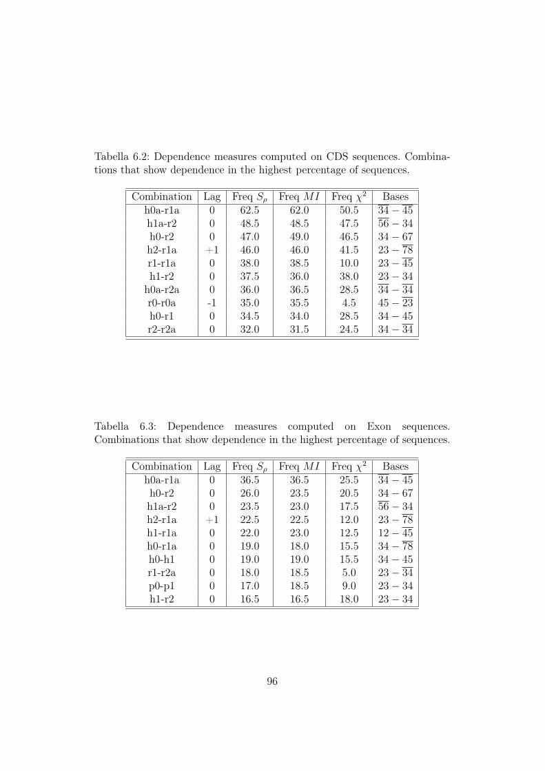
Tabella 6.2: Dependence measures computed on CDS sequences. Combina-tions that show dependence in the highest percentage of sequences.

Combination Lag Freq Sρ Freq MI Freq χ2 Basesh0a-r1a 0 62.5 62.0 50.5 34− 45h1a-r2 0 48.5 48.5 47.5 56− 34h0-r2 0 47.0 49.0 46.5 34− 67h2-r1a +1 46.0 46.0 41.5 23− 78r1-r1a 0 38.0 38.5 10.0 23− 45h1-r2 0 37.5 36.0 38.0 23− 34h0a-r2a 0 36.0 36.5 28.5 34− 34r0-r0a -1 35.0 35.5 4.5 45− 23h0-r1 0 34.5 34.0 28.5 34− 45r2-r2a 0 32.0 31.5 24.5 34− 34

Tabella 6.3: Dependence measures computed on Exon sequences.Combinations that show dependence in the highest percentage of sequences.

Combination Lag Freq Sρ Freq MI Freq χ2 Basesh0a-r1a 0 36.5 36.5 25.5 34− 45h0-r2 0 26.0 23.5 20.5 34− 67h1a-r2 0 23.5 23.0 17.5 56− 34h2-r1a +1 22.5 22.5 12.0 23− 78h1-r1a 0 22.0 23.0 12.5 12− 45h0-r1a 0 19.0 18.0 15.5 34− 78h0-h1 0 19.0 19.0 15.5 34− 45r1-r2a 0 18.0 18.5 5.0 23− 34p0-p1 0 17.0 18.5 9.0 23− 34h1-r2 0 16.5 16.5 18.0 23− 34

96

Introns

The analysis conducted on intron sequences indicates that no dichotomicclass combination shows a dependence in a number of sequences higher than20% (see Table 6.4). This indicates that there are no short-range dependencestructure as far as introns are concerned.

Once again Sρ and MI measures shows similar outcomes, while χ2 seemsto be less sensitive.

Tabella 6.4: Dependence measures computed on intron sequences.Combinations that show dependence in the highest percentage of sequences.

Combination Lag Freq Sρ Freq MI Freq χ2 Basesr2-r2a 0 18.5 17.5 4.0 12− 45h0a-r2a 0 17.5 17.0 12.0 34− 34r1- r2a 0 16.0 15.5 4.0 23− 34h0a-h1a 0 15.0 14.0 14.5 34− 56h0-r2 0 12.5 12.5 5.0 34− 67r0a-r2a 0 12.0 12.5 3.0 23− 34r0-r0a -1 11.5 11.5 2.5 45− 23h1a-r2 0 11.5 11.5 6.5 56− 34h0a-r1a 0 11.5 11.5 13.5 34− 45h0-r1 0 11.5 11.5 2.5 34− 45

97

Long introns

Table 6.5 shows the dichotomic class combinations with the highest depen-dence frequency. We can see that no combination exceed a 30% frequency.Dependence is more frequent in the couples r2-r2a and r1-r2a at lag 0 (around28% when computed with Srho and MI indexes). It could be argued thatRumer class is relevant in order to recognize different introns within the samegene.

It is interesting to notice that if we use χ2 as measure of dependence, nocombination shows a dependece frequency higher than 20%.

Tabella 6.5: Dependence measures computed on long intron sequences.Combinations that show dependence in the highest percentage of sequences.

Combination Lag Freq Sρ Freq MI Freq χ2 Basesr2-r2a 0 28.5 28.5 7.5 12− 45r1- r2a 0 26.5 28.0 5.5 23− 34h0a-r2a 0 24.0 24.5 13.5 34− 34r1-r1a 0 22.5 21.0 13.0 23− 45h0-r1 0 22.0 22.0 11.0 34− 45h1a-r2 0 22.0 22.0 6.5 56− 34h0a-h1a 0 21.0 20.5 18.5 34− 56r0-r1 -1 19.0 19.0 6.5 45− 23p0a-r1 -1 18.5 18.0 0 45− 23h1-r2 0 18.0 18.5 16.0 23− 34

98

UTRs

Dependence analysis on UTR sequences shows interesting results. In fact wecan see that only two combinations are dependent in more than 20% of thesequences: h0a-r1a and h0-h1, both at lag 0 (see Table 6.6) While the firstcombination is typical of coding sequences (it is indeed the more frequentboth in CDS and exons), the second one is specific of UTRs, since we havenot met it previously. Notice that both these two combinations involve bases3 and 4 on the first binary sting and bases 4 and 5 on the second binarystring. It is also interesting to underline that χ2 detects h0− h1 dependencestructure in 26% of the sequences, while it does not detect h0a-r1a with arate higher than 20%.

Tabella 6.6: Dependence measures computed on UTR sequences. Combina-tions that show dependence in the highest percentage of sequences.

Combination Lag Freq Sρ Freq MI Freq χ2 Basesh0-h1 0 29.0 29.0 26.0 34− 45h0a-r1a 0 28.5 30.0 17.0 34− 45h0-r2 0 19.0 20.0 6.0 34− 67h1-r1a 0 18.5 19.0 7.5 12− 45p1-p2 0 17.5 16.5 10.5 34− 445r0-r0a -1 16.5 16.0 0.5 45− 23h1a-r1a 0 15.5 16.0 7.0 23− 12h0a-r2a 0 15.0 14.0 5.5 34− 34p0-p2 0 13.5 14.0 1.5 23− 45h0-r2a 0 13.0 14.0 2.05 34− 67

99

Intergenes

Finally we can see that dependence analysis conducted on intergenes showssimilar results as UTRs. In fact all the dependence measures used detect a de-pendence structure in more than 20% of sequences only for the combinationh0-h1 at lag 0 (see Table 6.7). This could mean that there is a short-range de-pendence involving hidden class that is relevant in order to recognize portionsof DNA that are not genes or that do not undergo to translation process.

It is interesting to underline that the difference between UTRs and in-tergenes is in the combination h0a-r1a, detected as relevant in UTRs butnot in intergenes. This short-range dependence could discriminate betweennon coding region present within (UTRs) or outside (intergenes) genes, re-membering that it is present with the highest frequency both in CDS andexons.

Tabella 6.7: Dependence measures computed on intergenes sequences.Combinations that show dependence in the highest percentage of sequences.

Combination Lag Freq Sρ Freq MI Freq χ2 Basesh0-h1 0 26.0 28.0 23.0 34− 45h0-r2a 0 18.5 17.5 3.0 34− 67h0-h1a 0 18.0 18.0 15.5 34− 89h1-h2a -1 18.0 17.5 3.5 45− 45h0a-h2a -1 17.0 15.5 14.5 67− 45h1a-h2a +1 16.5 17.0 10.5 23− 45h1a-h2a -1 16.5 15.0 13.0 56− 12h0a-h2 +1 15.5 15.0 0.5 34− 56h0a-r2a 0 15.5 15.5 4.0 34− 34h2-r2a +1 14.5 14.5 0 23− 67

100

Tabella 6.8: Comparison between the dependence measures of the four maincombinations computed in all the genome portions

CDS Exon IntronCombination Lag Sρ MI χ2 Sρ MI χ2 Sρ MI χ2

h0a-r1a 0 62.5 62.0 50.5 36.5 36.5 25.5 11.5 10.0 13.5h1a-r2 0 48.5 48.5 47.5 23.5 23.0 17.5 11.5 13.0 6.5h0-r2 0 47.0 49.0 46.5 26.0 23.5 20.5 12.5 12.5 5.0h2-r1a +1 46.0 46.0 41.5 22.5 22.5 12.0 7.0 8.5 2.5

Long introns UTR IntergenesCombination Lag Sρ MI χ2 Sρ MI χ2 Sρ MI χ2

h0a-r1a 0 16.0 15.5 18.5 28.5 30.0 17.0 3.0 3.5 1.0h1a-r2 0 22.0 22.0 11.0 11.5 11.0 8.0 8.0 8.0 4.5h0-r2 0 16.5 17.0 4.0 19.0 20.0 6.0 2.0 2.5 2.5h2-r1a +1 16.0 16.5 6.0 7.5 7.0 2.0 4.0 4.5 1.5

101

6.2.2 Comparison between indexes

Sρ vs. Mutual information

Figure 6.1 shows the boxplots of the differences between the frequency ofrejections computed with Sρ and MI. We can see that the median is around0 for all the portion of the genome analyzed.

Moreover only few dichotomic class combinations display a differencegreater than 2.

Sρ vs. χ2

Looking at Figure 6.2 it is clear how Sρ detects dependence structure betterthan χ2.

A big group of dichotomic class combinations display differences greaterthan 10%, in particular when CDS are considered.

It is evident (and interesting) how χ2 index has difficulty in detectingdependence structures involving Rumer class variables.

Mutual information vs. χ2

If we compare MI and χ2 indexes we can observe big differences in detectingdependence structures as shown in Figure 6.3. Mutual information seemsto be more sensitive than χ2. Once again, a big group of dichotomic classcombinations display differences greater than 10%, in particular when CDSare considered.

6.2.3 Comments

The analysis shows that there is an important correlation between h0a andr1a at lag 0 in exon and, overall, in CDS.

• involves adjacent bases of the same codon.(12 and 23)

• the percentage of sequences that shows this correlation is remarkablyhigher in CDS than in exons.

The fact that we can find this short-range dependence only in coding se-quences could represent a clue supporting the hypothesis of the importanceof dichotomic class in error detection and correction mechanism.

There are at least other three combinations of dichotomic classes thatseem to show a relevant dependence in CDS:

• h1a and r2 at lag 0

102

Figura 6.1: Comparison between Sρ and MI ability of detecting dependencestructures.

103

Figura 6.2: Comparison between Sρ and χ2 ability of detecting dependencestructures.

104

Figura 6.3: Comparison between MI and χ2 ability of detecting dependencestructures.

105

• h0 and r2 at lag 0

• h2 and r1a at lag 1

All of these involve a Rumer and a hidden binary string as to indicatethat it is necessary an interaction between the two dichotomic class in orderto detect a dependence structure.

We can also see an important even though less frequent, dependence bet-ween h0 and h1 binary strings in UTRs and intergenes. This combinationseems to be specific for non coding regions external to the genome portionsthat undergo to transcription and translation processes.

Finally we can state that Sρ and MI indexes show a similar behaviour indetecting dependence structure in couples of binary sequences. χ2 index, in-stead, seem to be less sensitive: it, in fact, detect the same kind of dependencebut in a lower number of sequences.

6.3 Multiple testing problemIn this section I introduce the problem of multiple testing and describe somemethods that I could (and should) apply in order to adjust the type I errorrate. This is one of the main future developments of this research work.

Notice that Giannerini et al. [14] has applied such adjustment in a simi-lar analysis on different data. Their results show that there are dependencestructures similar to those presented here.

In this study I conducted a series of repeated tests on different groups ofsequences in order to assess the presence of dependence structures betweendichotomic classes binary strings. The use of repeated tests may lead to errorsin results interpretation. In fact, once the type I error rate is set at α = 5% foreach test, the chance of erroneously finding a statistically significant impact is5%. However, when the “family” of hypothesis tests are considered together,the “combined” type I error rate could be considerably larger than 5%.

For example, suppose that the null hypothesis is true for each test andthat tests are independent. Then, the chance of finding at least one spuriousimpact is 1− (1−α)N , where N is the number of tests. Thus, the probabilityof making at least one type I error is 23 % if 5 tests are conducted, 64% for20 tests, and so on as shown in Table 6.3.

The two most common definitions of the combined type I error rate foundin literature are the family-wise error rate (FWER) and the false discoveryrate (FDR):

106

Tabella 6.9: Chances of findings spurious impacts for independent tests

Number of independent tests Probabilty that at least one testwith true null hypotheses is statistically significant

5 0.2310 0.4020 0.6450 0.92

• The FWER, defined by Tukey [53] is the probability that at least onenull hypothesis will be rejected when all null hypotheses are true. Asdiscussed, the FWER is 1− (1− α)N , for independent tests, where Nis the number of tests.

• The FDR, defined by Benjamini and Hochberg [3], is a more recentapproach for assessing how errors in multiple testing could be conside-red. The FDR is the expected proportion of all rejected null hypothesesthat are rejected erroneously.

Table 6.10 helps clarify these two error rates. Suppose that multiple testsare conducted to assess intervention effects on N study outcomes and thatM null hypotheses are true (M is unobservable). Suppose further that basedon t-tests, Q null hypotheses are rejected and that A, B, C, and D signifycell counts when t-test results are compared to the truth. The counts Q andA to D are random variables.

Tabella 6.10: The number of errors when testing multiple hypotheses

Results from hypothesis tests(Observed)

Truth(Unobserved) H0 is not rejected H0 is rejected TotalH0 is true A B MH0 is false C D (N-M)Total (N-Q) Q N

In Table 6.10, the FWER is the probability that the random variable Bis at least 1 among the M null hypotheses that are true. The FDR equalsthe expected value of B /Q , where B /Q is defined to equal 0 if Q = 0.3

107

If all null hypotheses are true, then B = Q and the FDR and FWER areequivalent, otherwise the FDR is smaller than or equal to the FWER.

The two error rates have a different philosophical basis. The FWER mea-sures the likelihood of a single erroneous rejection of the null hypothesis acrossthe family of tests. FWER is concerned with mistakenly reporting any stati-stically significant findings. Unwarranted scientific conclusions about evalua-tion findings could be made as a result of even one mistake and that resear-chers may select erroneous significant findings for emphasis when reportingand publishing results.

The rationale behind the FDR is that a few erroneous rejections may notbe as problematic for drawing conclusions about the family tested when manynull hypotheses are rejected as they would be if only a few null hypothesesare rejected. The rejection of many null hypotheses is a signal that there arereal differences across the contrasted groups.

FDR is a less conservative measure than the FWER, especially if a con-siderable fraction of all null hypotheses are false. Thus, as reported below,methods that control the FDR could yield tests with greater statistical powerthan those that control the FWER. The choice of which error criterion tocontrol is important and must be made prior to the data analysis.

6.3.1 Statistical Solutions to the Multiple Testing Pro-blem

A large body of literature describes statistical methods to adjust type I errorsfor multiple testing ([?, 55, 56, 33]). The literature suggests that there is notone method that is preferred in all instances. Rather, the appropriate measurewill depend on the study design, the primary research questions that are tobe addressed, and the strength of inferences that are required.

Methods for FWER Control

Until recently, most of the literature on multiple testing focused on methodsto control the FWER at a given α level (that is, methods to ensure thatthe FWER ≤ α). The most well-known method is the Bonferroni procedure,which sets the significance level for individual tests at α/N where N is thenumber of tests.

The Bonferroni procedure controls the FWER when all null hypothe-ses are true or when some are true and some are false (that is, it providesstrong control of the FWER). The Bonferroni method applies to both conti-nuous and discrete data, controls the FWER when the tests are correlated,and provides adjusted confidence bounds (by using α/N rather than α in the

108

calculations). Furthermore, it is flexible because it controls the FWER fortests of joint hypotheses about any subset of N separate hypotheses (inclu-ding individual contrasts). The procedure will reject a joint hypothesis H0 ifany p-value for the individual hypotheses included in H0 is less than α/N .The Bonferroni method, however, yields conservative bounds on type I errorand, hence, has low power.

Many modified and sometimes more powerful versions of the Bonferronimethod have been developed that provide strong control of the FWER. Heresome examples are provided:

• Sidák (1967) [48] developed a slightly less conservative bound wherethe significance level for individual tests is set at 1− (1− α)1/N ratherthan α/N . This method has properties similar to those of the Bonfer-roni method and is slightly more powerful, although it does not controlthe FWER in all situations in which test statistics are dependent.

• Holm (1979) [31] developed a sequential step-down method : (1) or-der the p-values from the individual tests from smallest to largest,p1 ≤p2... ≤ pN , and order the corresponding null hypothesesH0(1), H0(2), ..., H0(N);(2) define k as the minimum j such that pj > α/(N − j + 1); and (3)reject all H0(j) for j = 1, ..., (k − 1). This procedure is more powerfulthan the Bonferroni method because the bound for this method se-quentially increases whereas the Bonferroni bound remains fixed. TheHolm method controls the FWER in the strong sense, but cannot beused to obtain confidence intervals.

• Hochberg (1988) [29] developed a step-up procedure that involves se-quential testing where p-values are ordered from largest to smallest(rather than vice versa as for the Holm test). The method first definesk as the maximum j such that pj ≤ α/(N − j + 1), and then rejec-ts all H0(j) for j = 1, ..., k. This procedure is more powerful than theHolm method, but the control of the FWER is not guaranteed for allsituations in which the test statistics are dependent (although simula-tion studies have shown that it is conservative under many dependencystructures).

• Bootstrap and permutation resampling methods are alternative, computer-intensive methods that provide strong control of the FWER ([56]).These methods incorporate distributional and correlational structuresacross tests, so they tend to be less conservative than the other general-purpose methods and, hence, may have more power. Furthermore, theyare applicable in many testing situations.

109

Methods for FDR Control

Benjamini and Hochberg ([3]) showed that when conducting N tests, thefollowing four-step procedure will control the FDR at the α level:

1. Conduct Nseparate t-tests, each at the common significance level α.

2. Order the p-values of the N tests from smallest to largest, where p1∗ ≤p2 ≤ ... ≤ pN are the ordered p-values.

3. Define k as the maximum j for which pj ≤j

Nα

4. Reject all null hypotheses H0(j)j = 1, 2, ..., k.. If no such kexists, thenno hypotheses are rejected.

This step-up sequential procedure, which has become increasingly popularin the literature, is easy to use because it is based solely on p-values from theindividual tests. Benjamini and Hochberg [3] first proved that this procedure(BH procedure) controls the FDR for continuous test statistics and Benjaminiand then proved that this procedure also controls the FDR for discrete teststatistics [4].

The original result was proved assuming independent tests correspondingto the true null hypotheses (although independence was not required fortest statistics corresponding to the false null hypotheses). More research isneeded to assess whether the BH procedure is robust when independence andpositive regression dependency are violated.

6.3.2 Related problems

There are two related concerns with the adjustment procedures discussedabove:

1. they result in tests with reduced statistical power

2. they could result in tests with even less power when the test statisticsare correlated (dependent).

Loss in Statistical Power

The statistical procedures that control for multiplicity reduce type I errorrates for individual tests. Consequently, these adjustment procedures resultin tests with reduced statistical power. the probability of rejecting the nullhypothesis given that the null hypothesis is false. Stated differently, these

110

adjustment methods reduce the likelihood that the tests will identify true dif-ferences between the contrasted groups. The more conservative the multipletesting strategy, the greater the power loss.

Multiplicity adjustments involve a trade-off between type I and type IIerror rates. Conservative testing strategies, such as the Bonferroni and similarmethods, can result in considerable losses in the statistical power of the tests,even if only a small number of tests are performed. The less conservative BHtest has noticeably more power if a high percentage of all null hypotheses arefalse.

Dependent Test Statistics

Individual test statistics are likely to be related in many situations.Some of the adjustment methods discussed above (such as the Bonferroni

and Holm methods) control the FWER at a given α level when tests arecorrelated. However, for some forms of dependency, these methods may adjustsignificance levels for individual tests by more than is necessary to controlthe FWER. This could lead to further reductions in the statistical power ofthe tests. For example, if test correlations are positive and large, each teststatistic is providing similar information about intervention effects, and thus,would likely produce similar p-values. Consequently, in these situations, feweradjustments to type I error rates are needed to control the FWER.

Finally, the BH method controls the FDR under certain forms of depen-dency and for certain test statistics, but not for others.

111

Capitolo 7

Conclusions

The objective of this thesis was to characterize the genome of the entire chro-mosome 1 of A.thaliana, a small flowering plants used as a model organism instudies of biology and genetics, on the basis of a recent mathematical modelof the genetic code.

First I have reviewed the main mathematical features of the model andits symmetry properties. Then, I have analyzed the whole chromosome 1 ofA.thaliana by creating specific routines that, by using genome annotations,extract and build seven groups of sequences: genes, exons, introns, codingsequences (CDS), intergenes, untranslated regions (UTR) and regulatory se-quences. Then I created fictitious sequences called long introns in order tohave a type of sequence to be compared with CDS.

The nucleotide sequences were then transformed into binary sequencesbased on the definition of the three different dichotomic classes: Rumer, hid-den and parity. So I generated 18 random variables corresponding to theproportion of 1 in each one of the binary string computed in and out of fra-me 1 and 2 on both the sense and the antisense strand . These 18 variables,along with the 4 variables relating to the proportions of A, C, G and T ofeach sequence, were used to conduct three different types of analysis.

First, it is carried out a descriptive analysis with the aim to characterizethe different portions of the genome on the basis of 22 variables describedabove. Results indicate the presence of regularities in each portion of thegenome considered. In particular intergenes, DNA sequences present betweentwo successive genes that have no apparent biological or regulating function,show an impressive regularity given by:

p ' 60% r ' 31% h ' 49%

112

in all binary sequences analyzed (computed on both the sense and the anti-sense strand, and undergone to all the transformations).

Moreover we can observe the presence of remarkable differences betweencoding sequences (CDS and exons) and non-coding sequences. Since meanvalues of dichotomic classes variables vary with frame only for coding se-quences, frame seems to be important only for them. This effect is higherin CDS than exons, suggesting a sort of “union effect” that occurs whenfragments of coding sequences (exons) join together to form a CDS.

For what concerns the specific role of each dichotomic class, we couldassume that parity class is important in order to distinguish between codingsequences in sense and antisense strand while Rumer and hidden classes seemto be useful in order to discriminate different kinds of non-coding sequences.In particular introns seem to minimize hidden class mean values.

In a second moment I wanted to verify if the dichotomic classes were able todiscriminate between the different portions of the genome. So I created a setof logistic regression models in order to discriminate between pairs of portionsof the genome using, as regressors, different combinations of the variablespreviously created. The results obtained show that dichotomic classes seem tobe useful in order to discriminate between coding and non-coding sequences,as to underline the importance of frame. Once again there seems to be a sortof ”union effect” that enhance, when we consider CDS, the features observedin exons. However I realized the use of dichotomic classes does not improve,almost always, the ability of discriminating different portions of the genomerespect to what is obtained using only proportion of bases.

Finally, I wanted to check the existence of short-range dependence betweenbinary sequences computed on the basis of the different dichotomic classes.I used three different measures of dependence: the well-known χ2 − test andtwo indices derived from the concept of entropy i.e. Mutual Information (MI)and Sρ, a normalized form of “Bhattacharya Hellinger Matusita distance”.The results obtained show that there is a significant short-range dependencestructure only for the coding sequences. This dependence involves in particu-lar CDS, highlighting once again the existence of a sort of ”union effect” whenthe exons join together to form a CDS. The existence of such a dependencestructure is a clue of an underlying error detection nd correction mechani-sm, whose biological bases are partly known (for example the proofreadingprocess by DNA polymerase).

I have also compared the results obtained using the different indices ofdependence. It is clear that both Sρ and mutual information are better than

113

χ2 in detecting dependence structures between binary sequences. All threeindices, in fact, reveal a dependence between the same combinations of dicho-tomic classes. However, MI and Sρ do it in a significantly higher percentageof sequences analyzed with respect to what χ2 do. However, it is not possibleto define which is the best between MI and Sρ as they seem to have the sameability to detect dependence structures .

In conclusion of my thesis work, I can say that the mathematical modelhere described is a useful tool for interpreting the different portions of thegenetic code of A.thaliana. Dichotomic classes seem in fact useful in discrimi-nating the coding portions of the genome (sequences which are transcribedand translated) from the non-coding ones. They also seem to characterizethe different non-coding portions of the genome. The presence of a short-range dependence structure and the enhanced effect that is observed in CDScompared to exons suggest that this mathematical structure of the geneticcode can be the basis of both the recognition of the different portions of co-ding sequences present within a same gene and the error detection/correctionmechanism.

No doubt, further studies are needed in order to assess how the infor-mation carried by dichotomic classes could discriminate between coding andnoncoding sequence and, therefore, contribute to unveil the role of the ma-thematical structure in error detection and correction mechanisms. Still, Ihave shown the potential of the approach presented for the understandingthe management of genetic information.

It will be interesting to perform the same type of analysis on the genomeof other organisms considered as models for studies of molecular biology andgenetics such as the nematode Caenorabditis elegans, the fruitfly Drosphilamelanogaster, the bacterium Escherichia coli and the mouse Mus musculus.

The main long term objective of this research is the understanding, ininformational terms, of the coding/decoding strategies that govern the accu-racy of genetic processing, with particular emphasis on the error detectionand correction mechanisms and its possible implementation in terms of dy-namical molecular machines. I believe that this approach could help to keepthe promises and hopes related to molecular biology and the Human GenomeProject.

114

Appendice A

Dichotomic class tables

115

A.1 Normal sequences

A.1.1 Median values

p0 r0 h0 p1 r1 h1 p2 r2 h2Genes 56.05 38.04 47.66 56.25 37.97 47.76 56.88 37.79 46.94CDS 50.25 43.88 51.85 51.57 41.04 54.84 58.78 38.23 45.94

Exons 52.00 41.94 50.82 52.63 39.62 52.00 56.52 38.98 47.54Introns 61.11 34.48 38.89 60.50 32.99 38.46 59.38 32.56 37.93

Long Int 60.44 33.42 41.07 60.29 33.16 40.94 60.00 33.13 40.78IG 60.85 30.59 49.42 60.82 30.56 49.40 60.84 30.54 49.35

UTR 60.00 34.58 43.61 60.00 34.55 43.57 60.00 34.55 43.66Reg 60.00 34.55 45.00 60.00 34.52 44.65 60.00 34.97 45.10

Tabella A.1: Median values of dichotomic class percentages computed in sensestrand for each sequence class

p0a r0a h0a p1a r1a h1a p2a r2a h2aGenes 56.80 37.55 51.36 56.88 38.15 51.32 56.52 37.85 51.15CDS 54.62 38.24 48.87 56.90 49.33 49.35 51.30 43.10 44.08

Exons 54.84 40.00 48.94 56.00 45.78 49.12 53.23 42.58 46.67Introns 60.61 29.17 60.82 61.54 26.76 61.54 61.71 28.57 61.29

Long Int 60.45 29.12 58.91 60.69 28.62 59.05 60.71 29.17 59.05IG 60.86 30.67 49.40 60.78 30.75 49.41 60.85 30.65 49.44

UTR 60.00 31.58 53.73 60.00 31.65 53.95 59.81 31.58 53.95Reg 60.00 32.69 50.46 60.00 33.33 50.23 59.00 32.35 50.00

Tabella A.2: Median values of dichotomic class percentages computed inantisense strand for each sequence class

116

A.1.2 Mean values


Exons 52.13 42.17 50.58 52.71 39.93 51.44 56.26 39.47 47.41Introns 61.21 34.85 38.74 60.40 33.06 38.33 59.29 32.82 37.83

Long Int 60.67 33.22 41.04 60.42 32.74 40.87 60.05 32.56 40.76IG 60.62 31.48 49.19 60.53 31.43 49.07 60.42 31.49 49.13

UTR 60.22 35.27 44.55 60.01 35.24 44.23 60.15 35.25 44.31Reg 59.67 35.86 44.08 59.72 35.84 43.56 60.19 36.53 43.45

Tabella A.3: Mean values of dichotomic class percentages computed in sensestrand for each sequence class


Exons 54.85 40.75 49.09 55.92 45.28 49.27 53.29 42.76 47.06Introns 60.45 29.38 61.01 61.58 26.75 61.68 61.74 28.64 61.36

Long Int 60.57 29.15 58.66 60.92 28.43 58.85 60.94 29.04 58.78IG 60.56 31.56 49.12 60.47 31.56 49.09 60.54 31.53 49.14

UTR 60.12 32.16 52.20 59.70 32.40 52.30 59.71 32.19 52.65Reg 60.39 32.61 49.50 59.74 33.28 48.97 59.18 33.15 49.13

Tabella A.4: Mean values of dichotomic class percentages computed inantisense strand for each sequence class

117

A.2 Complementary sequences

A.2.1 Median values


Exons 56.99 46.15 48.15 50.54 43.48 47.00 53.57 50.00 51.43Introns 59.38 30.43 61.11 60.71 30.30 61.54 60.87 30.30 62.07

Long Int 60.00 31.25 58.93 60.36 31.13 59.06 60.38 31.05 59.22IG 60.79 31.96 50.22 60.80 32.08 50.28 60.85 32.00 50.29

UTR 60.00 33.33 55.19 60.00 33.33 55.22 60.00 33.52 55.10Reg 60.00 33.33 52.09 60.00 33.64 51.82 60.00 33.45 51.69

Tabella A.5: Median values of dichotomic class percentages computed in sensestrand for each complement sequence class


Exons 51.35 43.33 50.00 54.05 42.86 50.00 57.89 46.81 52.63Introns 60.00 34.78 39.18 60.39 36.00 38.46 61.11 35.71 38.71

Long Int 60.29 35.25 41.09 60.46 35.48 40.95 60.66 35.42 40.95IG 60.77 31.89 50.25 60.87 31.95 50.22 60.77 31.92 50.19

UTR 60.00 36.64 45.24 60.00 36.36 45.00 60.00 36.54 44.93Reg 60.00 36.59 46.99 60.00 36.67 46.83 60.00 36.36 46.76

Tabella A.6: Median values of dichotomic class percentages computed inantisense strand for each complement sequence class

118

A.2.2 Mean values


Exons 56.68 46.36 48.08 50.94 44.24 47.10 53.60 50.05 51.13Introns 59.38 30.37 61.25 60.66 30.20 61.67 60.88 30.25 62.17

Long Int 60.09 30.84 58.96 60.52 30.78 59.13 60.53 30.84 59.24IG 60.56 32.64 50.00 60.46 32.70 50.03 60.68 32.67 49.97

UTR 59.98 33.95 53.82 60.09 33.99 54.00 60.10 34.11 53.92Reg 59.69 33.91 51.29 60.01 34.71 50.60 59.81 34.40 50.71

Tabella A.7: Mean values of dichotomic class percentages computed in sensestrand for each complement sequence class


Exons 51.72 43.59 50.08 54.12 43.32 49.83 57.55 46.78 52.04Introns 59.69 34.92 38.99 60.21 36.10 38.32 61.06 35.82 38.64

Long Int 60.19 34.58 41.34 60.52 34.93 41.15 60.83 34.86 41.22IG 60.64 32.51 50.05 60.61 32.62 49.97 60.44 32.62 49.93

UTR 59.63 37.18 46.23 59.95 36.96 45.98 59.82 36.97 45.62Reg 59.96 38.05 46.34 59.86 37.64 45.85 60.23 37.15 45.69

Tabella A.8: Mean values of dichotomic class percentages computed inantisense strand for each complement sequence class

119

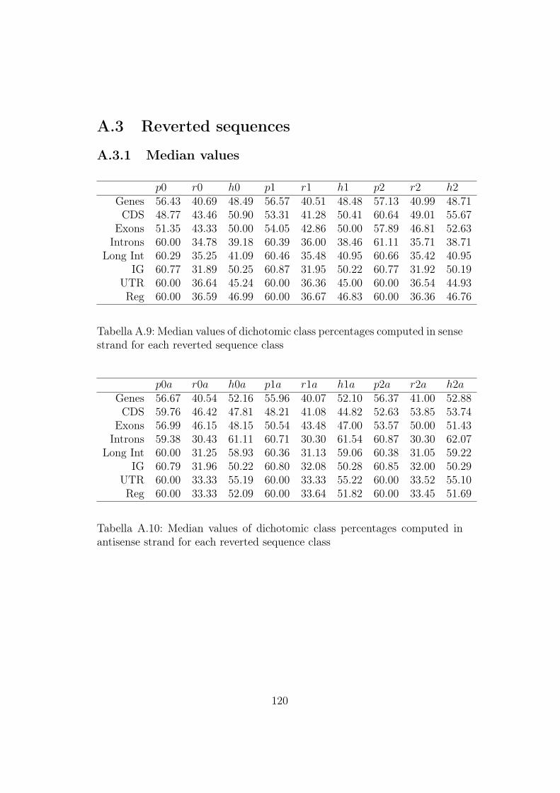
A.3 Reverted sequences

A.3.1 Median values


Exons 51.35 43.33 50.00 54.05 42.86 50.00 57.89 46.81 52.63Introns 60.00 34.78 39.18 60.39 36.00 38.46 61.11 35.71 38.71

Long Int 60.29 35.25 41.09 60.46 35.48 40.95 60.66 35.42 40.95IG 60.77 31.89 50.25 60.87 31.95 50.22 60.77 31.92 50.19

UTR 60.00 36.64 45.24 60.00 36.36 45.00 60.00 36.54 44.93Reg 60.00 36.59 46.99 60.00 36.67 46.83 60.00 36.36 46.76

Tabella A.9: Median values of dichotomic class percentages computed in sensestrand for each reverted sequence class


Exons 56.99 46.15 48.15 50.54 43.48 47.00 53.57 50.00 51.43Introns 59.38 30.43 61.11 60.71 30.30 61.54 60.87 30.30 62.07

Long Int 60.00 31.25 58.93 60.36 31.13 59.06 60.38 31.05 59.22IG 60.79 31.96 50.22 60.80 32.08 50.28 60.85 32.00 50.29

UTR 60.00 33.33 55.19 60.00 33.33 55.22 60.00 33.52 55.10Reg 60.00 33.33 52.09 60.00 33.64 51.82 60.00 33.45 51.69

Tabella A.10: Median values of dichotomic class percentages computed inantisense strand for each reverted sequence class

120

A.3.2 Mean values


Exons 51.72 43.59 50.08 54.12 43.32 49.83 57.55 46.78 52.04Introns 59.69 34.92 38.99 60.21 36.10 38.32 61.06 35.82 38.64

Long Int 60.19 34.58 41.34 60.52 34.93 41.15 60.83 34.86 41.22IG 60.64 32.51 50.05 60.61 32.62 49.97 60.44 32.62 49.93

UTR 59.63 37.18 46.23 59.95 36.96 45.98 59.82 36.97 45.62Reg 59.96 38.05 46.34 59.86 37.64 45.85 60.23 37.15 45.69

Tabella A.11: Mean values of dichotomic class percentages computed in sensestrand for each reverted sequence class


Exons 56.68 46.36 48.08 50.94 44.24 47.10 53.60 50.05 51.13Introns 59.38 30.37 61.25 60.66 30.20 61.67 60.88 30.25 62.17

Long Int 60.09 30.84 58.96 60.52 30.78 59.13 60.53 30.84 59.24IG 60.56 32.64 50.00 60.46 32.70 50.03 60.68 32.67 49.97

UTR 59.98 33.95 53.82 60.09 33.99 54.00 60.10 34.11 53.92Reg 59.69 33.91 51.29 60.01 34.71 50.60 59.81 34.40 50.71

Tabella A.12: Mean values of dichotomic class percentages computed inantisense strand for each reverted sequence class

121

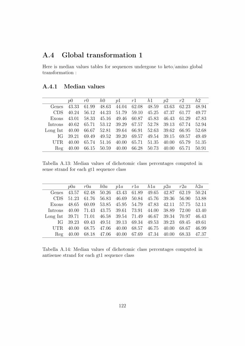
A.4 Global transformation 1Here is median values tables for sequences undergone to keto/amino globaltransformation :

A.4.1 Median values


Exons 43.01 58.33 45.16 49.46 60.87 45.83 46.43 61.29 47.83Introns 40.62 65.71 53.12 39.29 67.57 52.78 39.13 67.74 52.94

Long Int 40.00 66.67 52.81 39.64 66.91 52.63 39.62 66.95 52.68IG 39.21 69.49 49.52 39.20 69.57 49.54 39.15 69.57 49.49

UTR 40.00 65.74 51.16 40.00 65.71 51.35 40.00 65.79 51.35Reg 40.00 66.15 50.59 40.00 66.28 50.73 40.00 65.71 50.91

Tabella A.13: Median values of dichotomic class percentages computed insense strand for each gt1 sequence class


Exons 48.65 60.09 53.85 45.95 54.79 47.83 42.11 57.75 52.11Introns 40.00 71.43 43.75 39.61 73.91 44.00 38.89 72.00 43.40

Long Int 39.71 71.01 46.58 39.54 71.49 46.67 39.34 70.97 46.43IG 39.23 69.43 49.51 39.13 69.34 49.53 39.23 69.45 49.61

UTR 40.00 68.75 47.06 40.00 68.57 46.75 40.00 68.67 46.99Reg 40.00 68.18 47.06 40.00 67.69 47.34 40.00 68.33 47.37

Tabella A.14: Median values of dichotomic class percentages computed inantisense strand for each gt1 sequence class

122

A.4.2 Mean values


Exons 43.32 58.13 45.47 49.06 60.61 46.13 46.40 60.86 48.08Introns 40.62 65.47 53.21 39.34 67.23 52.84 39.12 67.47 52.95

Long Int 39.91 66.89 52.43 39.48 67.36 52.33 39.47 67.54 52.40IG 39.44 68.68 49.46 39.54 68.75 49.52 39.32 68.68 49.55

UTR 40.02 65.11 51.35 39.91 65.15 51.53 39.90 65.15 51.49Reg 40.31 65.00 51.49 39.99 65.26 51.75 40.19 64.71 51.62

Tabella A.15: Mean values of dichotomic class percentages computed in sensestrand for each gt1 sequence class


Exons 48.28 59.60 53.11 45.88 55.36 47.84 42.45 57.64 51.37Introns 40.31 71.27 43.31 39.79 73.91 43.58 38.94 72.02 42.90

Long Int 39.81 71.06 46.24 39.48 71.79 46.36 39.17 71.17 46.09IG 39.36 68.60 49.52 39.39 68.60 49.68 39.56 68.65 49.68

UTR 40.37 68.21 46.58 40.05 67.98 46.16 40.18 68.21 46.32Reg 40.04 68.15 46.20 40.14 67.74 45.87 39.77 68.05 45.66

Tabella A.16: Mean values of dichotomic class percentages computed inantisense strand for each gt1 sequence class

123

A.5 Global transformation 2Here is median values tables for sequences undergone to purine/pyrimidineglobal transformation :

A.5.1 Median values


Exons 48.00 54.10 53.57 47.37 57.14 52.94 43.48 50.00 50.82Introns 38.89 70.21 44.44 39.50 70.37 44.68 40.62 70.37 44.44

Long Int 39.56 68.89 46.64 39.71 69.05 46.78 40.00 69.07 46.72IG 39.15 68.14 50.34 39.18 68.00 50.33 39.16 68.10 50.35

UTR 40.00 66.67 48.18 40.00 66.67 47.95 40.00 66.67 47.95Reg 40.00 66.67 48.15 40.00 66.67 47.51 40.00 66.67 47.46

Tabella A.17: Median values of dichotomic class percentages computed insense strand for each gt2 sequence class


Exons 45.16 56.97 44.44 44.00 57.69 50.00 46.77 53.49 46.21Introns 39.39 65.45 53.68 38.46 64.29 53.57 38.29 64.52 53.91

Long Int 39.55 64.85 52.90 39.31 64.60 52.78 39.29 64.63 53.02IG 39.14 68.18 50.33 39.22 68.13 50.34 39.15 68.14 50.23

UTR 40.00 63.64 52.24 40.00 63.92 52.55 40.19 63.64 52.17Reg 40.00 63.71 51.06 40.00 63.93 50.53 41.00 64.29 50.87

Tabella A.18: Median values of dichotomic class percentages computed inantisense strand for each gt2 sequence class

124

A.5.2 Mean values


Exons 47.87 54.00 53.08 47.29 56.46 52.33 43.74 50.35 50.37Introns 38.79 70.28 44.02 39.60 70.44 44.30 40.71 70.40 44.19

Long Int 39.33 69.37 46.68 39.58 69.43 46.76 39.95 69.36 46.69IG 39.38 67.51 50.21 39.47 67.46 50.12 39.58 67.50 50.08

UTR 39.78 66.44 47.67 39.99 66.40 47.39 39.85 66.30 47.43Reg 40.33 66.90 46.41 40.28 66.26 45.58 39.81 66.65 45.71

Tabella A.19: Mean values of dichotomic class percentages computed in sensestrand for each gt2 sequence class


Exons 45.15 56.73 44.93 44.08 57.28 50.07 46.71 53.59 46.54Introns 39.55 65.40 53.92 38.42 64.23 53.55 38.26 64.52 54.24

Long Int 39.43 65.52 52.87 39.08 65.18 52.73 39.06 65.24 52.99IG 39.44 67.64 50.18 39.53 67.53 50.00 39.46 67.56 50.00

UTR 39.88 63.20 52.39 40.30 63.40 52.72 40.29 63.41 52.56Reg 39.61 62.77 51.22 40.26 63.44 50.81 40.82 63.78 51.02

Tabella A.20: Mean values of dichotomic class percentages computed inantisense strand for each gt2 sequence class

125

Appendice B

Distributions

126

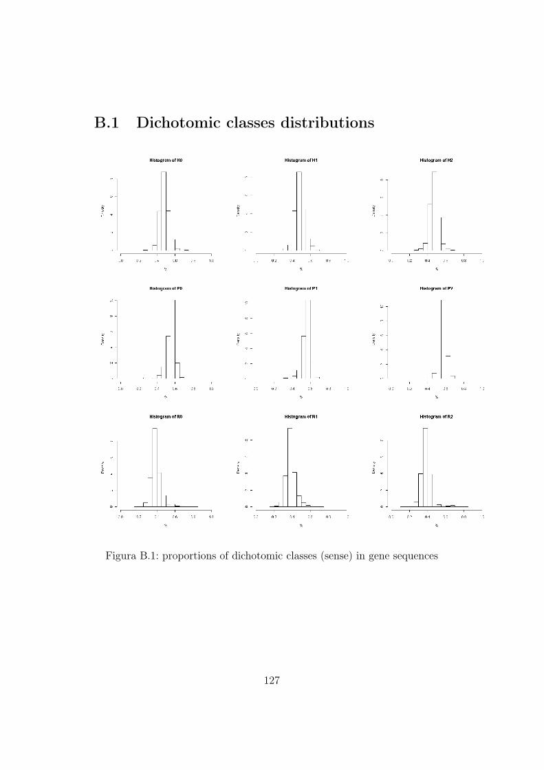
B.1 Dichotomic classes distributions

Figura B.1: proportions of dichotomic classes (sense) in gene sequences

127

Figura B.2: proportions of dichotomic classes (sense) in intergene sequences

128

Figura B.3: proportions of dichotomic classes (sense) in exon sequences

129

Figura B.4: proportions of dichotomic classes (sense) in CDS sequences

130

Figura B.5: proportions of dichotomic classes (sense) in intron sequences

131

Figura B.6: proportions of dichotomic classes (sense) in long intron sequences

132

Figura B.7: proportions of dichotomic classes (sense) in UTR sequences

133

Figura B.8: proportions of dichotomic classes (sense) in regulatory sequences

134

Figura B.9: proportions of dichotomic classes (antisense) in gene sequences

135

Figura B.10: proportions of dichotomic classes (antisense) in intergenesequences

136

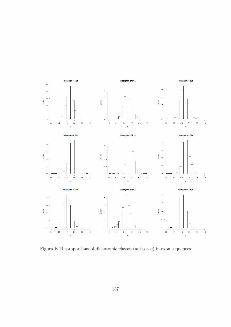
Figura B.11: proportions of dichotomic classes (antisense) in exon sequences

137

Figura B.12: proportions of dichotomic classes (antisense) in CDS sequences

138

Figura B.13: proportions of dichotomic classes (antisense) in intron sequences

139

Figura B.14: proportions of dichotomic classes (antisense) in long intronsequences

140

Figura B.15: proportions of dichotomic classes (antisense) in UTR sequences

141

Figura B.16: proportions of dichotomic classes (antisense) in regulatorysequences

142

B.2 Base distribution

Figura B.17: proportions of bases in gene sequences

143

Figura B.18: proportions of bases in intergene sequences

144

Figura B.19: proportions of bases in exon sequences

145

Figura B.20: proportions of bases in coding sequences (CDS)

146

Figura B.21: proportions of bases in intron sequences

147

Figura B.22: proportions of bases in long intron sequences

148

Figura B.23: proportions of bases in UTR sequences

149

Figura B.24: proportions of bases in regulatory sequences

150

Bibliografia

[1] F.J. Aherne, N.A. Thacker, and P.I. Rockett. The bhattacharyya metricas an absolute similarity measure for frequency coded data. Kybernetika,34(4):363–368, 1998.

[2] E.G. Baek and W.A. Brock. A non parametric test for independence ofa multivariate time series. Statistica Sinica, 1992.

[3] Y. Benjamini and Y. Hochberg. Controlling the false discovery rate: apractical and powerful approach to multiple testing. Journal of the RoyalStatistical Society. Series B (Methodological), pages 289–300, 1995.

[4] Y. Benjamini and D. Yekutieli. The control of the false discovery ratein multiple testing under dependency. Annals of statistics, pages 1165–1188, 2001.

[5] B.K. Bhattacharya and G.T. Toussaint. An upper bound on the pro-bability of misclassification in terms of matusita’s measure of affinity.Annals of the Institute of Statistical Mathematics, 34(1):161–165, 1982.

[6] T.M. Cover and J.A. Thomas. Elements of information theory. Wiley-interscience, 2006.

[7] F. Crick. Central dogma of molecular biology. Nature, 1970.

[8] Francis Crick. ”Chapter 8: The genetic code”. What mad pursuit: apersonal view of scientific discovery. New York: Basic Books, 1988.

[9] G.A. Darbellay and D. Wuertz. The entropy as a tool for analysingstatistical dependences in financial time series. Physica A: StatisticalMechanics and its Applications, 287(3):429–439, 2000.

[10] A. Dionísio, R. Menezes, and D.A. Mendes. Entropy-based independencetest. Nonlinear Dynamics, 44(1):351–357, 2006.

151

[11] B. Efron. Large-scale inference: empirical Bayes methods for estimation,testing, and prediction, volume 1. Cambridge University Press, 2010.

[12] M. Fernandes and B. Neri. Nonparametric entropy-based tests ofindependence between stochastic processes. Econometric Reviews, 2010.

[13] S. Giannerini, D. L. Gonzalez, and R. Rosa. Dichotomic classes andshort range dependence in coding sequences. In Second InternationalWorkshop on “Mathematical models for the genetic information”.

[14] S. Giannerini, E. Maasoumi, and E.B. Dagum. Bulletin of theInternational Statistical Institute, 56th Session, 2007.

[15] D. L. Gonzalez. Can the genetic code be mathematically described?Medical Science Monitor, 10(4):11–17, 2004.

[16] D. L. Gonzalez. Error detection and correction codes. In M. Barbieriand J. Hoffmeyer, editors, The Codes of Life: The Rules of Macroevo-lution, volume 1 of Biosemiotics, chapter 17, pages 379–394. SpringerNetherlands, 2008.

[17] D. L. Gonzalez. The mathematical structure of the genetic code. InM. Barbieri and J. Hoffmeyer, editors, The Codes of Life: The Rulesof Macroevolution, volume 1 of Biosemiotics, chapter 8, pages 111–152.Springer Netherlands, 2008.

[18] D. L. Gonzalez, S. Giannerini, and R. Rosa. Detecting structure inparity binary sequences: Error correction and detection in DNA. IEEEEngineering in Medicine and Biology Magazine, 25:69–81, 2006.

[19] D. L. Gonzalez, S. Giannerini, and R. Rosa. Strong short-range correla-tions and dichotomic codon classes in coding DNA sequences. PhysicalReview E, 78(5):051918, 2008.

[20] D. L. Gonzalez, S. Giannerini, and R. Rosa. The mathematical structureof the genetic code: a tool for inquiring on the origin of life. Statistica,LXIX(3–4):143–157, 2009.

[21] D.L. Gonzalez, S. Giannerini, and R. Rosa. Circular codes revisited: Astatistical approach. Journal of Theoretical Biology, 275(1):21–28, 2011.

[22] D.L. Gonzalez, S. Giannerini, and R. Rosa. On the origin of themitochondrial genetic code. Working paper, 2012.

152

[23] C.W. Granger and J.L. Lin. Using the mutual information coefficientto identify lags in nonlinear models. Journal of Time Series Analysis,15(4):371–384, 1994.

[24] C.W. Granger, E. Maasoumi, and J.C. Racine. A dependence metric forpossibly nonlinear processes. Journal of Time Series Analysis, 2004.

[25] S.G. Gregory, K.F. Barlow, and et al. The dna sequence and biologicalannotation of human chromosome 1. Nature, 2006.

[26] W.M. Griffiths, J.H. Miller, D.T. Suzuki, and al. An Introduction toGenetic Analysis (7th ed.). W. H. Freeman., 2000.

[27] Joseph M. Hilbe. Logistic Regression Models. Chapman & Hall/CRCPress, 2009.

[28] Y. Hochberg. A sharper bonferroni procedure for multiple tests ofsignificance. Biometrika, 75(4):800–802, 1988.

[29] W. Hoeffding. A non parametric test of independence. Annals ofmathematical statistics, 1948.

[30] S. Holm. A simple sequentially rejective multiple test procedure.Scandinavian journal of statistics, pages 65–70, 1979.

[31] D.W. Hosmer and S. Lemeshow. Applied Logistic Regression. Wiley,2000.

[32] J. Hsu. Multiple comparisons: theory and methods. Chapman &Hall/CRC, 1996.

[33] S. Ihara. Information theory for continuous systems, volume 2. WorldScientific Publishing Company Incorporated, 1993.

[34] The Arabidopsis Genome Initiative. Analysis of the genome sequence ofthe flowering plant arabidopsis thaliana. Nature, 2000.

[35] Berg J, Tymoczko J.L., and Stryer L. Biochemistry (6th ed.). W. H.Freeman, 2006.

[36] D. Johnson and R. McClelland. A general dependence test andapplications. Journal of Applied Econometrics, 1998.

153

[37] E.S. Lander, L.M. Linton, B. Birren, C. Nusbaum, M.C. Zody, J. Bald-win, K. Devon, K. Dewar, M. Doyle, W. FitzHugh, et al. Initial sequen-cing and analysis of the human genome. Nature, 409(6822):860–921,2001.

[38] B. Lewin. Genes Ix. Jones and Bartlett Publishers Sudbury, MA, USA:,2008.

[39] W. Li. Mutual information functions versus correlation functions.Journal of statistical physics, 60(5):823–837, 1990.

[40] E. Maasoumi and J. Racine. Entropy and predictability of stock marketreturns. Journal of Econometrics, 107(1):291–312, 2002.

[41] M.Nirenberg. Deciphering the genetic code. Office of NIH History, 2010.

[42] P.K. Mulligan, R. C. King, and W.D. Stansfield. A dictionary ofgenetics. Oxford University Press, 2006.

[43] H. Pearson. Genetics: What is a gene? Nature, 441(7092):398–401, 2006.

[44] E. Pennisi. Dna study forces rethink of what it means to be a gene.Science, 316(5831):1556–1557, 2007.

[45] J. Pinske. A consistent nonparametric test for serial independenc. Journlof Econometrics, 1998.

[46] E. Shannon. A mathematical theory of evidence: Bellsyt. Techn.Journal, 27:379–423, 1948.

[47] Z. Šidák. Rectangular confidence regions for the means of multivariatenormal distributions. Journal of the American Statistical Association,62(318):626–633, 1967.

[48] H.J. Skaug and D. Tjostheim. Testing for serial independence usingmeasures of distance between densities. Lecture notes in statistics -New York - Springer Verlag-, pages 363–377, 1996.

[49] D. Swarbreck, C. Wilks, P. Lamesch, T.Z. Berardini, M. Garcia-Hernandez, H. Foerster, D. Li, T. Meyer, R. Muller, L. Ploetz, et al.The arabidopsis information resource (tair): gene structure and functionannotation. Nucleic acids research, 36(suppl 1):D1009–D1014, 2008.

[50] R.D.C. Team et al. R: A language and environment for statisticalcomputing. R Foundation Statistical Computing, 2008.

154

[51] D. Tjostheim. Measues of dependence and tests for independence.Statistics, 1996.

[52] J.W. Tukey. The problem of multiple comparisons. Mimeographed Notes.

[53] J.C. Venter, M.D. Adams, E.W. Myers, P.W. Li, R.J. Mural, G.G. Sut-ton, H.O. Smith, M. Yandell, C.A. Evans, R.A. Holt, et al. The sequenceof the human genome. Science Signalling, 291(5507):1304, 2001.

[54] P.H. Westfall, R.D. Tobias, and R.D. Wolfinger. Multiple comparisonsand multiple tests using SAS. Sas Inst, 2011.

[55] P.H. Westfall and S.S. Young. Resampling-based multiple te-sting: Examples and methods for p-value adjustment, volume 279.Wiley-Interscience, 1993.

[56] E. Zeckendorf. Représentation des nombres naturels par une somme denombres de fibonacci ou de nombres de lucas. Bull. Soc. Roy. Sci. Liege,41:179–182, 1972.

155

Documents

Genome characterization through a mathematical model of the genetic code