Embed Size (px)
Citation preview

Genetic

Issued by Sandia National Laboratories, operated for the United States Department of Energy by Sandia Corporation.
NOTICE: This report was prepared as an account of work sponsored by an agency of the United States Government. Neither the United States Government, nor any agency thereof, nor any of their employees, nor any of their contractors, subcontractors, or their employees, make any warranty, express or implied, or assume any legal liability or responsibility for the accuracy, completeness, or usefulness of any information, apparatus, product, or process disclosed, or represent that its use would not infringe privately owned rights. Reference herein to any specific commercial product, process, or service by trade name, trademark, manufacturer, or otherwise, does not necessarily constitute or imply its endorsement, recommendation, or favoring by the United States Government, any agency thereof, or any of their contractors or subcontractors. The views and opinions expressed herein do not necessarily state or reflect those of the United States Government, any agency thereof, or any of their contractors.
Printed in the United States of America. This report has been reproduced directly from the best available copy.
Available to DOE and DOE contractors from U.S. Department of Energy Office of Scientific and Technical Information P.O. Box 62 Oak Ridge, TN 3783 1
Telephone: (865)576-8401 Facsimile: (865)576-5728 E-Mail: [email protected] Online ordering: http://www.doe.gov/bridge
Available to the public from U.S. Department of Commerce National Technical Information Service 5285 Port Royal Rd Springfield, VA 22 161
Telephone: (800)553-6847 Facsimile: (703)605-6900 E-Mail: [email protected] Online order: http: / / www.ntis.gov/ordering. htm

SAND2000-2846Unlimited Release
Printed November 2000
Development and Application of Genetic AlgorithmsFor Sandia’s RATLER Robotic Vehicles
Daniel W. BarnetteParallel Computational Sciences Department
Richard J. PryorEvolutionary Computing Methods
John T. FeddemaIntelligent Systems Sensors & Controls
Sandia National LaboratoriesPO Box 5800
Albuquerque, New Mexico 87185-0316
ABSTRACT
This report describes the development and application of genetic algorithms for thepurpose of directing robotic vehicles to various signal sources. The use of such vehiclesfor surveillance and detection operations has become increasingly important in defenseand humanitarian applications. The computationally parallel programming model asimplemented on Sandia’s parallel compute cluster Siberia and used to develop the geneticalgorithm is discussed in detail. The model generates a computer program that, whenloaded into a robotic vehicle’s on-board computer, is designed to guide the robot tosuccessfully accomplish its task. A significant finding is that a genetic algorithm derivedfor a simple, steady state signal source is robust enough to be applied to much morecomplex, time-varying signals. Also, algorithms for significantly noisy signals werefound to be difficult to generate and should be the focus of future research. Themethodology may be used for a genetic programming model to develop trackingbehaviors for autonomous, micro-scale robotic vehicles.

2
Acknowledgments
The authors wish to acknowledge the following:
Funding for this project was obtained through Sandia’s Laboratory Directed Researchand Development (LDRD) office (Project 10690, Task 03).
Johnny Hurtado, Department 15211, supplied the mathematical models for the signalsources.
Wolfram Research’s Mathematica 4.0 was used to generate signal source and simulatedrobot path illustrations.

3
Contents
Acknowledgments 2
Introduction 4
The Genetic Algorithm 5
Program Representation of the Genetic Algorithm 7
Problem Setup 8
Signal Source Models 9
Results 9A. Simulation: Genetic Algorithm for Non-Noisy Signal Sources 9B. Field Test: Coupling the Genetic Algorithm with Sandia’s RATLERs 10C. Simulation: Non-Noisy Genetic Algorithm Applied to Noisy Signals 12D. Simulation: Genetic Algorithm for Noisy Signal Sources 12
Summary and Conclusions 13
References 13
Tables1. Functions and Terminals Available for Genetic Algorithm Decision Tree 62. Equations for Signal Source Models 93. Configuration of Sandia’s Parallel Compute Clusters 10
Figures1. Example of a 5-node, 3-level decision tree representing y=2.3 + 5.9x.2. Select, top-view convergence sequences of a representative genetic algorithm.3. Sandia’s parallel compute cluster, ALASKA/SIBERIA.4. Various source signal models used.5. Peak movement for the various signal source models.6. Simulated vehicle movement for the signal source models.7. Image of a typical RATLER vehicle.8. Model 0 source illustrating algorithmic convergence for 5% signal noise and non-
convergence for 8% signal noise.
AppendicesA – CEDAR Pseudo-Code Program ListingB – ROBOCOP.C Program ListingC – ROBOCOP.C Sample Output Listing for Model 0D – Mathematica 4.0 Graphics Program Listing
Distribution

4
Development and Application of Genetic AlgorithmsFor Sandia’s RATLER Robotic Vehicles
Introduction
The emerging technical approach to deal with a challenging, possibly hostile,environment is likely to involve a large number of small, but fairly intelligent, robots. Itis envisioned that these can covertly infiltrate a designated area, enter buildings, gatherappropriate information, and communicate with and learn from each other. They wouldalso communicate with a smaller number of on-the-scene soldiers backed up by powerfuloff-line computers that can carry out large-scale information collection, analyses, andsimulations. Each robot would have on-board electronics, ground-positioning andcommunication equipment, an obstacle detector, and some source-analysis capability.Each robot would also have a motor, wheels, and a motor control system. Although thedeployed robots would behave autonomously, each robot would communicateinformation with other robots during the task.
This report documents the effort to generate and apply a robust genetic algorithm to actas a vehicle controlling program for robotic behavior. In a typical scenario, robots areinitially distributed randomly in a field and given the goal of locating the emitting source,be it sound or smell. An onboard processor running the algorithm provides instructions tothe motor control system that directs the robot to the source location while navigatingaround obstacles.
The controlling algorithm is generated by a computer code designed to assemble, test,and compare many similar algorithms simultaneously. The code uses trial and error,tournament play, and best fits to generate a decision tree appropriate for the task. Oncechosen, the decision tree then becomes the controlling algorithm of choice. The algorithmin decision-tree form is then translated into high-level computer language such asFORTRAN or C, compiled, and downloaded to the robotic vehicles deployed in the task.The robotic vehicles are then controlled by execution of the code using onboardprocessors, sensors, and memory.
The Sandia RATLER robotic vehicle serves as a research platform for the current effort.Although the RATLER’s size precludes its large-scale use at present, further researchwill see the capabilities of RATLER reduced to micro-scale vehicles. Operationally, it isenvisioned that tens to hundreds of these small robots would be deployed to complete agiven task.

5
The Genetic Algorithm
Building a genetic algorithm is a compute-intensive process by virtue of the fact that itcontinually attempts to create successive generations of more fit algorithms.Improvement occurs in discrete steps called generations. A generation is composed of apopulation of individual algorithms each of which is a complete computer program. Thenumber of algorithms considered at one time varies based on the problem; however,hundreds, if not thousands, of genetic algorithms can be considered simultaneously byjudicious use of parallel computers. Typically, some algorithms will be more effectivethan others at doing the prescribed task. Each algorithm is scored for applicability, and itsfitness is given a numerical score such that the higher the fitness, the better the algorithm.The goal is to generate an algorithm that correctly solves the problem of interest.However, there is no guarantee that the chosen algorithm is necessarily the best – usually,it suffices.
To create subsequent generations, genetic operators of selection, reproduction, crossover,and mutation are used. The purpose of selection is to choose an algorithm from thecurrent population. In general, this algorithm will be better than most, but it may not bethe very best. Reproduction moves a selected algorithm directly into the next generation.Crossover uses the selection operator twice to select two algorithms from the currentpopulation that will be combined in some way to form a hybrid algorithm that will beplaced in the next generation. Mutation uses the selection operator once to choose analgorithm that will be changed in some way and placed in the next generation. The fourgenetic operators are discussed in more detail by Koza[1] and Pryor[2]. The developmentdescribed above proceeds across many generations until a single algorithm is found thatmeets a convergence criteria. This algorithm is then tested and, if found to be sufficientlyrobust, implemented as the robotic controlling program.
Pryor[2] gives an example of the program representation of a decision tree making up agenetic algorithm. The basic building block of a tree is called a node, with all nodes inthe tree having the same fixed structure. The first element of a node specifies the nodetype, which can either be a function or a terminal. A function node performs amathematical or Boolean operation and generally has branches (nonzero pointers) thatpoint to other nodes. The number of branches depends on the kind of function, e.g., add,subtract, multiply. A terminal node normally returns a value, does not have any branches(all pointers are zero), and terminates that section of the tree. Other elements within anode are a value position and pointers to other nodes. All of the nodes result in a decisiontree that performs a specified task. More detail is given in the next section.
Noise can have a significant impact in actual applications where genetic algorithms areemployed. Unless noise is accounted for during its creation, the genetic algorithm maynot be able to respond in an appropriate manner. Such was the case in the presentapplications, as will be shown.
Table 1 lists functions allowed to make up the genetic algorithm.

No.
FUNC 1 2 3 4 5 6
7 8 9 10 11
12
TERM 13 14 15 16 17 18 19
20
21
22 23
24
25 26 27 28 29 30 31 32 33 34 35 36
Table 1: Functions and Terminals Available for Genetic Algorithm Decision Tree
Function Name Mathematical Expression Comments
TIONS:RETURN Returns a valueADD + Adds two valuesSUBTRACT - Subtracts two valuesMULTIPLY * Multiplies two valuesIFGTEQ IF (value1 >= value2) Compares two valuesCOMPUTE ANGLE Determines which direction robot
facesSTORE A-REG Register for each robotSTORE B-REG Register for each robotSTORE C-REG Register for each robotINTEGER ROUND value=FLOOR(value1+0.5) Round to nearest integer valueSTORE AVG X-REG (1 - κ)*(AVG X-REG)
+ κ*(AVG X-REG)Exponential moving average for valuestored (κ=0.5)
STORE AVG Y-REG (1 - κ)*(AVG Y-REG) + κ*(AVG Y-REG)
Exponential moving average for valuestored (κ=0.5)
INALS:NEIGH 1 XPOS First nearest neighbor’s X locationNEIGH 2 XPOS Second nearest neighbor’s X locationNEIGH 1 YPOS First nearest neighbor’s Y locationNEIGH 2 YPOS Second nearest neighbor’s Y locationROBUG XPOS X location of robotROBUG YPOS Y location of robotROBUG DIRECTION 1=North, 2=East, 3=South,
4=WestDirection heading of robot (1,2,3, or4) on grid
NEIGH 1 SIGNAL Signal detected by first nearestneighbor
NEIGH 2 SIGNAL Signal detected by second nearestneighbor
ROBUG SIGNAL Signal detected by robotV-WALL XPOS North-South wall’s X location of
cornerV-WALL YPOS North-South wall’s Y location of
cornerH-WALL XPOS East-West wall’s X location of cornerH-WALL YPOS East-West wall’s Y location of cornerRECALL A-REG Use A-register’s contentsRECALL B-REG Use B-register’s contentsRECALL C-REG Use C-register’s contentsTURN NORTH Directs robot to face NorthTURN EAST Directs robot to face EastTURN SOUTH Directs robot to face SouthTURN WEST Directs robot to face WestTURN RIGHT Directs robot to turn rightMOVE AHEAD Directs robot to move aheadVALUE Store a value
6
7
Program Representation of the Genetic Algorithm
This section describes how the genetic algorithm is represented by individual programelements that make up a decision tree. The representation should always allow completeflexibility in defining programs, yet it must also ensure that the performance of thegenetic operations is not too cumbersome. A tree-like structure best meets theserequirements.
The basic building block of a tree is called a node, with all nodes in the tree having thesame fixed structure. The first element of a node specifies the node type, which can eitherbe a function or a terminal. A function node performs a mathematical or Booleanoperation and generally has branches (nonzero pointers) that point to other nodes. Thenumber of branches depends on the kind of function, e.g., add, subtract, multiply. Aterminal node normally returns a value, does not have any branches (all pointers arezero), and terminates that section of the tree. Other elements within a node are a valueposition and pointers to other nodes.
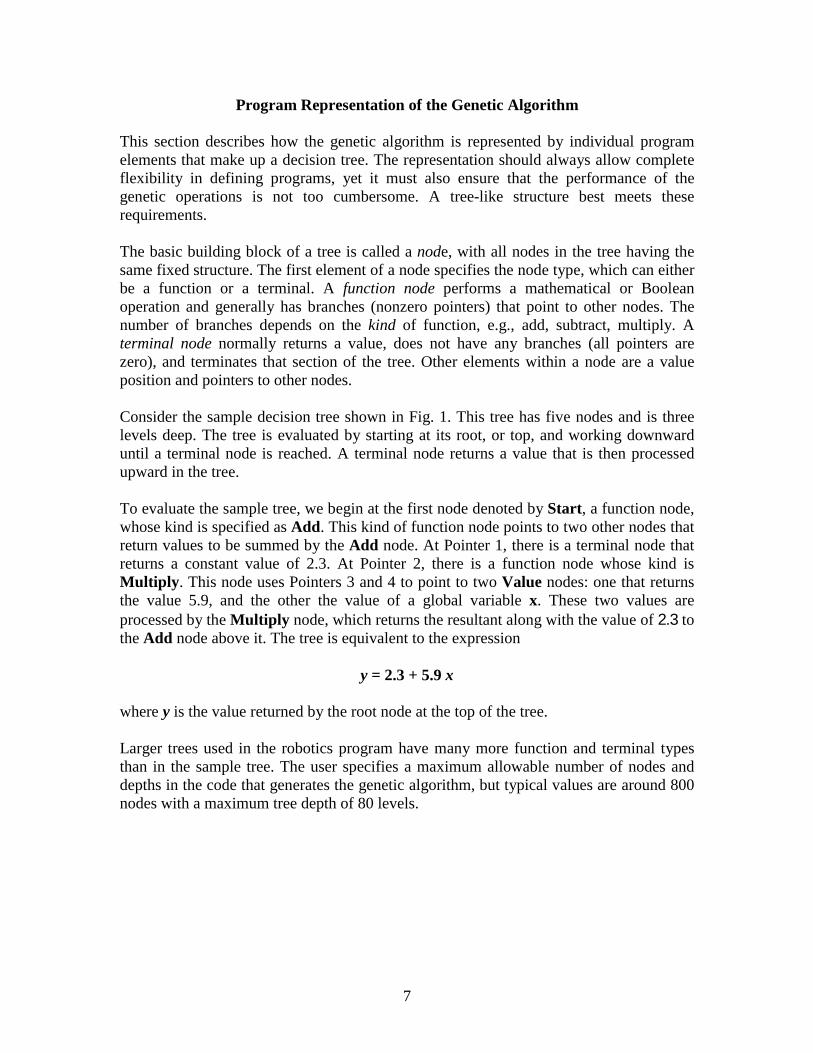
Consider the sample decision tree shown in Fig. 1. This tree has five nodes and is threelevels deep. The tree is evaluated by starting at its root, or top, and working downwarduntil a terminal node is reached. A terminal node returns a value that is then processedupward in the tree.
To evaluate the sample tree, we begin at the first node denoted by Start, a function node,whose kind is specified as Add. This kind of function node points to two other nodes thatreturn values to be summed by the Add node. At Pointer 1, there is a terminal node thatreturns a constant value of 2.3. At Pointer 2, there is a function node whose kind isMultiply. This node uses Pointers 3 and 4 to point to two Value nodes: one that returnsthe value 5.9, and the other the value of a global variable x. These two values areprocessed by the Multiply node, which returns the resultant along with the value of 2.3 tothe Add node above it. The tree is equivalent to the expression
y = 2.3 + 5.9 x
where y is the value returned by the root node at the top of the tree.
Larger trees used in the robotics program have many more function and terminal typesthan in the sample tree. The user specifies a maximum allowable number of nodes anddepths in the code that generates the genetic algorithm, but typical values are around 800nodes with a maximum tree depth of 80 levels.
8
Problem Setup
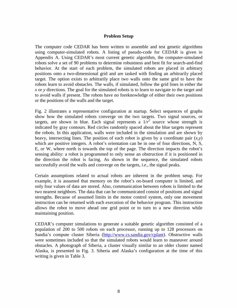
The computer code CEDAR has been written to assemble and test genetic algorithmsusing computer-simulated robots. A listing of pseudo-code for CEDAR is given inAppendix A. Using CEDAR’s most current genetic algorithm, the computer-simulatedrobots solve a set of 90 problems to determine robustness and best fit for search-and-findbehavior. At the start of each problem, the simulated robots are placed in arbitrarypositions onto a two-dimensional grid and are tasked with finding an arbitrarily placedtarget. The option exists to arbitrarily place two walls onto the same grid to have therobots learn to avoid obstacles. The walls, if simulated, follow the grid lines in either thex or y directions. The goal for the simulated robots is to learn to navigate to the target andto avoid walls if present. The robots have no foreknowledge of either their own positionsor the positions of the walls and the target.
Fig. 2 illustrates a representative configuration at startup. Select sequences of graphsshow how the simulated robots converge on the two targets. Two signal sources, ortargets, are shown in blue. Each signal represents a 1/r2 source whose strength isindicated by gray contours. Red circles randomly spaced about the blue targets representthe robots. In this application, walls were included in the simulation and are shown byheavy, intersecting lines. The position of each robot is given by a coordinate pair (x,y)which are positive integers. A robot’s orientation can be in one of four directions, N, S,E, or W, where north is towards the top of the page. The direction impacts the robot’ssensing ability: a robot is programmed to only sense an obstruction if it is positioned inthe direction the robot is facing. As shown in the sequence, the simulated robotssuccessfully avoid the walls and converge on the targets, i.e., the signal peaks.
Certain assumptions related to actual robots are inherent in the problem setup. Forexample, it is assumed that memory on the robot’s on-board computer is limited, andonly four values of data are stored. Also, communication between robots is limited to thetwo nearest neighbors. The data that can be communicated consist of positions and signalstrengths. Because of assumed limits in the motor control system, only one movementinstruction can be returned with each execution of the behavior program. This instructionallows the robot to move ahead one grid point or to turn to a new direction whilemaintaining position.
CEDAR’s computer simulations to generate a suitable genetic algorithm consisted of apopulation of 200 to 500 robots on each processor, running up to 128 processors onSandia’s compute cluster Siberia (http://www.cs.sandia.gov/cplant). Obstructive wallswere sometimes included so that the simulated robots would learn to maneuver aroundobstacles. A photograph of Siberia, a cluster visually similar to an older cluster namedAlaska, is presented in Fig. 3. Siberia and Alaska’s configuration at the time of thiswriting is given in Table 3.

9
Signal Source Models
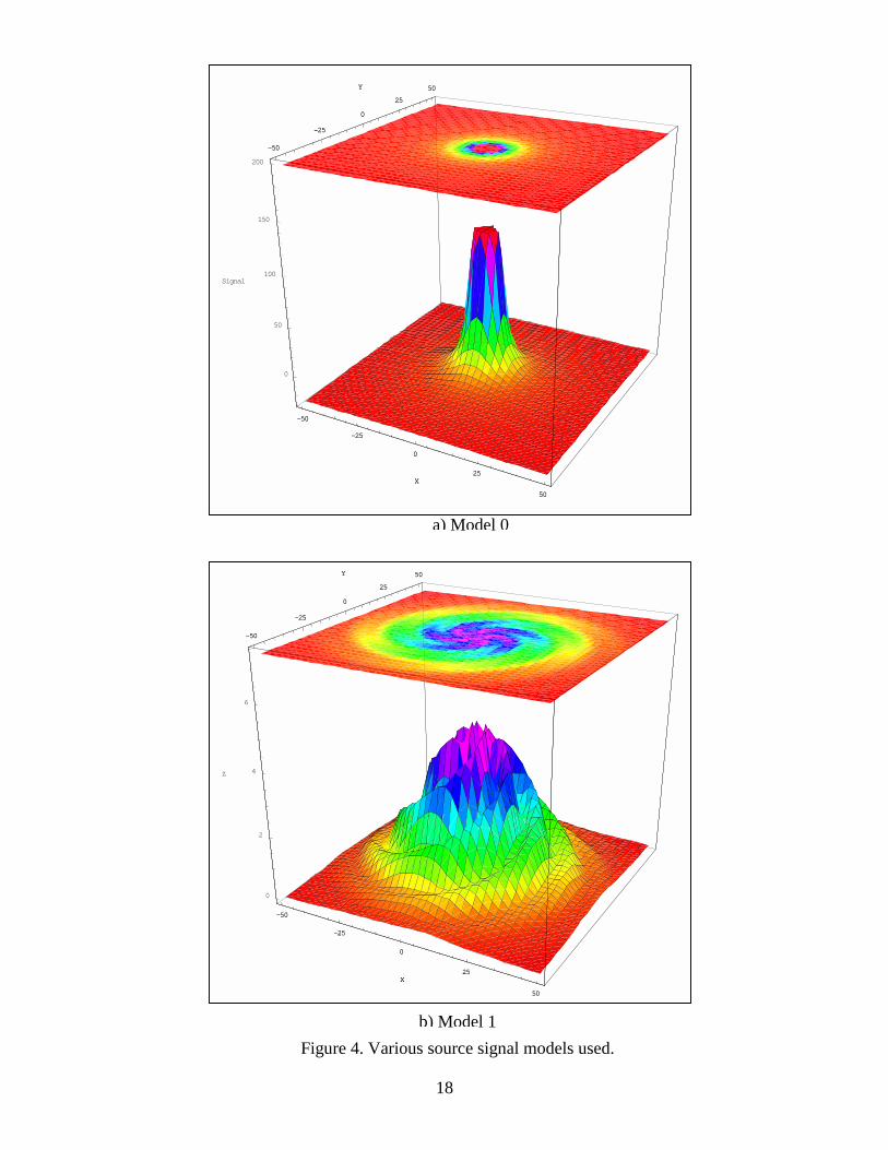
A total of four signal source models were considered. The equations governing each aregiven in Table 2. Mathematical representations of the models, generated usingMathematica[3], are shown in Fig. 4. The simplest model, Model 0, consists of a 1/r2
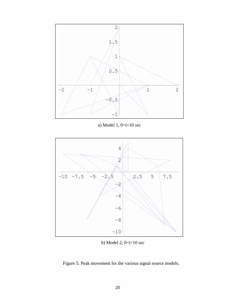
steady-state signal, as illustrated in Fig. 4a. Three time- and spatially-varying modelswere also considered. Illustrated in Figs. 4b, c, and d are Models 1, 2, and 3, respectively.Each of these functions has multiple local peaks that move around considerably as therobots search for the most likely signal peak. A sample of the maximum-peak movementfor the unsteady models is given in Figs. 5a, b, and c.
Results
A. Simulation: Genetic Algorithm for Non-Noisy Signal Sources
The first attempts at generating genetic algorithms centered on modeling each signalsource model. Wall-like obstructions were placed randomly on the grid so that thesimulated robots would learn to maneuver around them. This became a verycomputationally intensive process since the signal sources for Models 1, 2, and 3 weretime-varying and complicated, especially near the multiple center peaks.
Various attempts were made to accelerate the convergence. For example, more functions,such as exponential and sinusoidal, were added to the code from which the geneticalgorithm would be generated. The reasoning behind this approach was that if thealgorithm needed an exponential function that would otherwise be built from Taylor-series-like terms, for example, then adding this function to the list of possible functions to
Table 2. Equations for Signal Source Models
Model # Equation(s)0 2/1 r1 ]4)520[cos(
22 −−++− − tre r θπ2 ]4)45cos()410cos([cos
22 −−−− − ttre r θπ
3
]4)44cos()42cos([cos2
1)100
( 2
22
−−−−−−
tytxeyx
ππσ
σ , 0≥x
and
]4)44cos()42cos([cos2
1)( 2
22
−−−−−−
tytxey
x
ππσ
σ , 0<x
where
22 yxr += , )arctan(x
y=θ , t = time, and 22 += xσ
10
be chosen would negate the necessity to buproved to be slowly convergent, possiblycomplexity to the simpler algorithm being choices to the list of available functions algeof options from which to choose as a deciscould be considered for use in each node in aalgorithm became extremely tedious.
To alleviate the convergence problems, the aof using the algorithm generated for the smodels. No walls were simulated since it waswould not initially contain obstructions.
Simulated vehicle movement using the gengenerated using the code ROBOCOP, listegenerated by CEDAR is inserted in the funAppendix B, to complete the code. SampAppendix C. The Mathematica program used Appendix D.
The Model 0 result is illustrated in Fig. 6algorithm to the remaining models is showalgorithm worked very well for all signals foa surprising result considering the complexityHowever, further thought leads one to conclusteady-state signals may well be sufficient esources as long as sampling rates are high rela
B. Field Test: Coupling the Genetic Algorith
The rovers used in the field tests were SandRover (RATLER) vehicles. Typical RATLERare approximately the size of two shoeboxes p
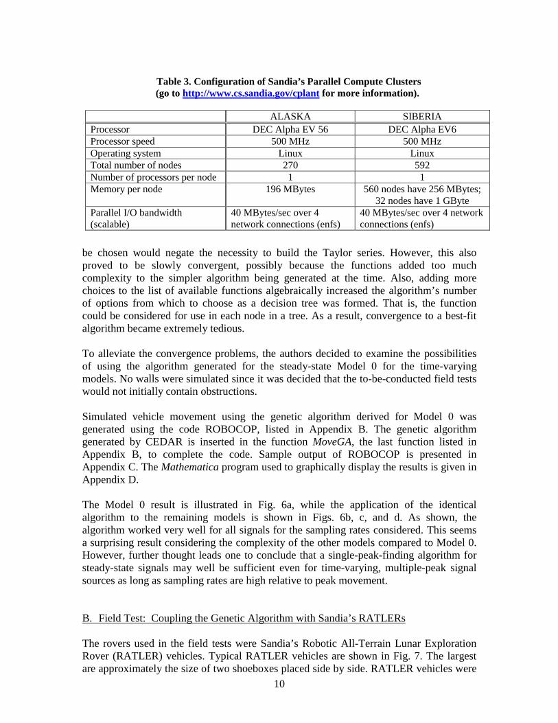
Table 3. Configuration of San(go to http://www.cs.sandia.go
ALProcessor DEC AProcessor speed 500Operating system LTotal number of nodesNumber of processors per nodeMemory per node 196
Parallel I/O bandwidth(scalable)
40 MBytes/snetwork conn
dia’s Parallel Compute Clustersv/cplant for more information).
ASKA SIBERIAlpha EV 56 DEC Alpha EV6 MHz 500 MHzinux Linux270 592
1 1MBytes 560 nodes have 256 MBytes;
32 nodes have 1 GByteec over 4 40 MBytes/sec over 4 network
ild the Taylor series. However, this also because the functions added too muchgenerated at the time. Also, adding morebraically increased the algorithm’s numberion tree was formed. That is, the function tree. As a result, convergence to a best-fit
uthors decided to examine the possibilitiesteady-state Model 0 for the time-varying decided that the to-be-conducted field tests
etic algorithm derived for Model 0 wasd in Appendix B. The genetic algorithmction MoveGA, the last function listed inle output of ROBOCOP is presented into graphically display the results is given in
a, while the application of the identicaln in Figs. 6b, c, and d. As shown, the
r the sampling rates considered. This seems of the other models compared to Model 0.de that a single-peak-finding algorithm forven for time-varying, multiple-peak signaltive to peak movement.
m with Sandia’s RATLERs
ia’s Robotic All-Terrain Lunar Exploration vehicles are shown in Fig. 7. The largestlaced side by side. RATLER vehicles were
ections (enfs) connections (enfs)

11
developed by Sandia as a prototype vehicle for a lunar mission. Each vehicle is typicallyequipped with an Intel 486 computer, differential GPS receiver, spread spectrum two-way packet radio, electronic compass and tilt sensors, video camera, and RF videotransmitter. Three RATLERs of the type shown in Fig. 7a were used during the tests.This was the minimum number needed for vehicle-to-vehicle communications asprovided for in the genetic algorithm.
The base station equipment with which the RATLERs stay in constant communicationconsists of a Pentium laptop computer, spread spectrum two-way packet radio,differential GPS base receiver, RF video receiver, and a battery power source. Theequipment is contained within a small trailer for mobility. The base station sendscommands and queries to the RATLERs over the packet radio. The communicationnetwork is configured as a token ring. Hence, if the base station becomes non-functional,the vehicles will continue to communicate. Also, if either the vehicle or base stationmisses its turn to communicate, communications can be re-established after a specifieddelay.
During field tests, the operator places the RATLERs in autonomous navigation mode. Alive video image from one of the vehicles can be displayed on the laptop along with thecurrent position of the vehicle on a Geographic Information System (GIS) map. MultipleRATLERs are driven to operator-specified set points using differential GPS and amagnetic compass, where they are allowed to navigate on their own to the source usingthe genetic algorithm controlling program. The positioning accuracy of the vehicles istypically 1 meter.
As a result of its success in finding the peaks of all signal models, the algorithm forModel 0 was implemented on robotic rovers for field tests. The signal source was a loudspeaker placed in a large field so as to closely simulate the 1/r2 Model 0 source. TheRATLERs were placed in a random position about the source. The genetic algorithmpreviously loaded into the RATLERs onboard memory was then executed and thevehicles were allowed to move about as directed by the algorithm. No obstructions wereplaced between the rovers and signal source.
Direct observations of the ensuing test were that the vehicles found the source butwandered significantly beforehand. The wandering was attributed to signal noise thatmay have been caused by nearby vehicle traffic, wind, and possibly electronic componenttolerances. Signal noise was not due to vehicle movement since signals were generatedonly after each RATLER stopped momentarily. Base station equipment recorded thenoise to be as high as 10% of the signal source. Noise was not modeled in the initialalgorithm for Model 0.
It was also discovered that a RATLER acting alone showed nearly identical behavior tothat when all three were attempting to locate the target. This apparently indicated that thevehicles were not communicating with each other even though provisions such asregisters were made available with the functions given in Table 1. Computer simulationsusing only one simulated robot reinforced the conclusion that the vehicles were notcommunicating as originally believed. Implications are that the vehicles were acting

12
autonomously and not collectively, as should be in the case of a swarm of vehicles. It isunknown why this occurred, but it is certainly an area for future research.
C. Simulation: Non-Noisy Genetic Algorithm Applied to Noisy Signals
Noise was introduced into the signal source used in Model 0’s simulator. The originalgenetic algorithm was then used to perform a post-mortem simulation and analysis of thefield tests. A random number generator was used to perturb the original signal within auser-specified percentage at each time step. This would hopefully reveal the effects ofnoise on the robot convergence path.
Results of the robot convergence path are illustrated in Fig. 8. Shown in Fig. 8a is theconvergence path for a 5% noise signal. The simulated rover finds the peak even thoughthe signal strength is slightly perturbed. However, an 8% perturbation causes thesimulated rover to never converge, as illustrated in Fig. 8b. Thus, the genetic algorithmfor Model 0 is apparently robust enough to handle small perturbations to around 5%.However, higher perturbations cause the robot to wander as observed in the field test.
At this point, two alternatives became obvious to alleviate the wandering. The firstapproach was to lower the signal noise in some way. This was quickly abandoned, sincethe factors causing the noise levels were out of the operators’ control. It is also possiblethat higher noise levels may exist during actual future applications and that these levelscould not be predicted beforehand.
The second approach was to introduce noise in the code that generates the geneticalgorithm.
D. Simulation: Genetic Algorithm for Noisy Signal Sources
It was thought that the genetic algorithm for Model 0 could be regenerated with theability to process noisy signals. The new algorithm, if successful, would allow the roversto find valid signal peaks even through a ‘dirty’ signal. Once again, so as not to add morecomplexity to the problem, walls were not modeled.
Significant computer time was spent on this approach, but without much success. Projectdeadlines prevented a thorough attack on this problem, but preliminary analyses indicatedsimulated rovers would find their way to a fairly large distance from the peak, and nocloser. It is not entirely understood why this happened. However, better convergencemight be achieved if the algorithm ensured each rover communicated with some of itsnearest neighbors, thereby triangulating the signal source. As has been discussed, rover-to-rover communications were apparently not occurring in the original Model 0 geneticalgorithm. Hence, another area of research should include a study of the ability of geneticalgorithms to intelligently process noisy signals.
13
Summary and Conclusions
This report documents a research effort in which a genetic algorithm code was developedand ported to Sandia’s parallel compute clusters. The code was modified to use the MPImessage passing protocol. Efficiency was improved by reducing excessive messagepassing between the master node and slave nodes. The ability to investigate time-varyingsignal sources was added to the original code. Visualization schemes were developed andimplemented for investigating simulated robot behavior before running field tests withactual hardware.
The result of this effort, a genetic algorithm, has been implemented in hardware as arobot controlling program. Field tests were conducted using Sandia’s RATLER roboticvehicles attempting to locate a low humming stereo speaker. Tests were successful,though significant wandering was observed that was not evident during computersimulations. This behavior is believed to be due to signal noise. Project deadlinesprevented generating a genetic algorithm that could filter noise and locate the peakefficiently. It was also noticed that the algorithm resulted in autonomous, rather thancollective, robot behavior. The factors that govern this behavior should be a topic offuture research.
An interesting finding of this research was the fact that a genetic algorithm developed fora simple test case proved very robust for more complex applications and signals.Computer simulations showed that the algorithm developed for a simple 1/r2 case provedsufficient for much more complicated applications. This should be kept in mind in anyfuture research involving applying genetic algorithms to complicated applications: keep itas simple as possible. Extensions of simple algorithms may be possible for much morecomplicated applications.
In conclusion, the authors believe genetic algorithms have a strong future at Sandia,especially when applied to problems that have no definitive analytical answers, but wherea ‘good’ solution will do. Future areas of research should include an approach thatensures rover-to-rover communications and the study of the effects of noisy signals onobtaining acceptable rover behavior. It is hoped that this report gives impetus toadditional research in these areas so that more robust genetic algorithms may bedeveloped.
References
1. Koza, J. R., Genetic Programming, On the Programming of Computers by Meansof Natural Selection, MIT Press, 1992.
2. Pryor, R. J., “Developing Robotic Behavior Using a Genetic ProgrammingModel,” SAND98-0074, Sandia National Laboratories, Albuquerque, NewMexico, January 1998.
3. Wolfram, S., The Mathematica Book, 3rd edition, Wolfram Media & CambridgeUniversity Press, 1996.

14
[Intentionally Left Blank]

Start
Pointer 1
Figure 1. Example of a 5-node, 3
Add01200
Pointer 2
Value2.30000
15
Pointer 3
-level decision tree
Multiply03400
Pointer 4
Value5.90000
representing y=2
Value of x00000
.3 + 5.9x.

WALLS
TARGETS
SIMULATEDROBOTS
a) Step 0
b) Step 36
c) Step 84
Figure 2. Select, top-view convergence sequences of a representative genetic algorithm.
16
17
Figure 3. Sandia’s parallel compute cluster, ALASKA/SIBERIA. For moredetails, go to web site http://www.cs.sandia.gov/cplant.
50Y 50Y
-50
-25
0
25
50
X
-50
-25
0
25
0
50
100
150
200
Signal
-50
-25
0
25
50
X
-50
-25
0
25
25
50Y
25
50Y
-50
-25
0
X
-50
-25
0
0
2
4
6
Z
-50
-25
0
X
-50
-25
0
Figure 4. Various
a) Model 0
25
50
25
50
b) Model 1
18
source signal models used.

19
-50
-25
0
25
50
X
-50
-25
0
25
50Y
0
2
4
6
Z
-50
-25
0
25
50
X
-50
-25
0
25
50Y
-50
-25
0
25
50
X
-50
-25
0
25
50
Y
0
0.5
1
1.5
Z
-50
-25
0
25
50
X
0
0.5
1
1.5
Z
d) Model 3
c) Model 2
Figure 4. Concluded
20
-2 -1 1 2
-1
-0.5
0.5
1
1.5
2
a) Model 1, 0<t<10 sec
-10 -7.5 -5 -2.5 2.5 5 7.5
-10
-8
-6
-4
-2
2
4
b) Model 2, 0<t<10 sec
Figure 5. Peak movement for the various signal source models.

21
- 1 1 2 3
- 3
- 2
- 1
1
2
3
c) Model 3, 0<t<10 sec
Figure 5. Concluded.

22
10.2 seconds
-50
-25
0
25
50
X-50
-25
0
25
50
Y
0
50
100
150
200
Signal
-50
-25
0
25
50
X
a) Model 0, t=10.2 sec
20.2 se conds
-50
-25
0
25
50
X
-50
-25
0
25
50
Y
0
2
4
6
Z
-50
-25
0
25
50
X
0
2
4
6
Z
b) Model 1, t=20.2 sec
Figure 6. Simulated vehicle movement for the signal source models.

23
15.1 seconds
-50
-25
0
25
50
X
-50
-25
0
25
50
Y
0
2
4
6
Z
-50
-25
0
25
50
X
0
2
4
6
Z
c) Model 2, t=16.1 sec
15.1 seconds
-50
-25
0
25
50
X
-50
-25
0
25
50
Y
0
0.5
1
1.5
Z
-50
-25
0
25
50
X
0
0.5
1
1.5
Z
d) Model 3, t=15.1 sec
Figure 6. Concluded.

Figure 7. RATLER vehicles devel
a)
2
o
b)4
ped at Sandia National Laboratories.

25
20.2 seconds
-50
-25
0
25
50
X-50
-25
0
25
50
Y
0
50
100
150
200
Signal
-50
-25
0
25
50
X
20.2 seconds
-50
-25
0
25
50
X-50
-25
0
25
50
Y
0
50
100
150
200
Signal
-50
-25
0
25
50
X
a) 5% signal noise
b) 8% signal noise
Figure 8. Model 0 source illustrating algorithmic convergence for 5% signal noise andnon-convergence for 8% signal noise.

26
[Intentionally Left Blank]

A-1
Appendix ACEDAR Pseudo-Code Program Listing
> # include Header files
> Define global variables
> #define Constants and parameters
1) main (unsigned int argc, char *argv[]) {
� Initialize Message Passing Interface (MPI) environment� if (NodeNum == 0 )� HandleNodeZero();� else� HandleOtherNodes();}
2) void HandleNodeZero () {
� Print initialized quantities� Call ReadList{} to read the best tree, if output from previous run� Call randomng{} to generate random number� Loop over the number of generations:� Loop over number of compute nodes� Wait for incoming trees to node zero� Check each incoming tree for fitness; if best, replace previous tree� If maximum number of generations reached, send message to all nodes to quit� Write the best tree to disk� Return to main}
3) void HandleOtherNodes () {
� Initialize trees, parameters� Call randomng{} to generate random number� Loop over population size
o Determine and store best tree on current compute node� Loop over number of generations
o Implement mutation, reproduction, crossover to generate new treeo Define current best tree
� Send best tree to node zero� Quit searching for best tree when node 0 says maximum number of generations
reached� Return to main
}
4) double EvalTree (AtomType *ptr, long ntsx) {
� Loop over number of tests to run to determine best treeso Define wall positions if usedo Define initial target position; initial robot positions
� Loop over number of cycles to be done for each test� Loop over number of robots

A-2
o Determine signal strength measured by each roboto Determine each robots’ nearest robot neighborso Move the robots according to current genetic algorithmo End loop over cycles
� Determine the distance the robots are from the target� End loop over tests� Determine the fitness of each tree� Return the fitness value
}
5) AtomType * GetBestTree (AtomType *bestIndiv) {� Receive the best tree from compute Node 0
}
6) void KillNodes () {� Kill all compute nodes when finished
}
7) OSErr InitManager () {� Initialize dynamic memory allocation
}
8) AtomType * myMalloc (void) {� Initialize memory allocated for trees
}
9) void myFree(AtomType *ptr) {� point to next location of free memory block
}
10) void HandleError (int errAction, OSErr err, char *script) {� Error handling routine for CEDAR
}
11) double RandomDouble ( double start, double stop ) {� Determine random number to type double precision
}
) 12) long RandomLong (long istart, long istop) {� Determine random number to type long
}
) 13) double randomng(int *pp) {� Random number generator
}
) 14) double eval (AtomType *ptr, RoBugType *bug) {� Compute the value of each tree node using assigned functionals
}
) 15) long TreeSize (AtomType *ptr) {� Compute the number of nodes in each tree structure
}
A-3
) 16) void CountNode (AtomType *ptr) {� Count and set points for each node
}
) 17) long TreeDepth (AtomType *ptr) {� Determine the number of levels of each tree
}
) 18) void NodeDepth (AtomType *ptr) {� Determine depth of each tree node
}
) 19) void DeleteOffspring (AtomType *ptr) {� Free memory from tree nodes no longer needed
}
) 20) AtomType * DuplicateTree (AtomType *fromptr) {� Duplicate a tree node using CopyNode
}
) 21) void CopyNode (AtomType *fromptr, AtomType *ptr) {� Free a block of memory� Copy a tree node from one block of memory to another
}
) 22) AtomType * CrossOver (AtomType *ptr1, AtomType *ptr2) {� Perform crossover algorithm on two tree nodes’ offspring
}
) 23) void PrintTree (AtomType *ptr) {� Print size and depth of tree to appropriate output file
}
) 24) void PrintNode (AtomType *ptr) {� Print tree nodes
}
) 25) AtomType * GenerateTree () {� Initialize maximum depth of initial tree
}
) 26) void GenNode (AtomType *ptr) {� Randomly generate tree nodes
}
) 27) void WriteCProgram (AtomType *ptr, long progIndex) {� Output initialization information formatted in C
}
) 28) void ArrayNode (AtomType *ptr, long nsize) {� determine memory pointers for tree nodes
}

A-4
) 29) void WriteCProgramNode (AtomType *ptr, FILE *ProgramFP) {� Output tree nodes formatted in C
}
) 30) void WriteFProgram (AtomType *ptr, long progIndex) {� Output initialization information formatted in FORTRAN
}
) 31) void WriteFProgramNode (AtomType *ptr, FILE *ProgramFP) {� Output tree nodes formatted in FORTRAN
}
) 32) long SelectTree (double fitness[]) {� Determine which tree is best
}
) 33) AtomType * TreeToList (AtomType *ptr) {� Determine absolute to relative memory address for each node
}
) 34) void ListNode (AtomType *ptr) {� Determine pointer values for each tree’s nodes
}
) 35) void AbsToRelAdr(AtomType *ptr, long size) {� Determine node’s relative address, given absolute address
}
) 36) void RelToAbsAdr (AtomType *ptr, long size) {� Determine node’s absolute address, given relative address
}
) 37) void WriteList (AtomType *ptr, long listIndex) {� Open and write list file
}
) 38) AtomType * ReadList (char ListFileName[]) {� Open and read list file
}
) 39) void MutateTree (AtomType *ptr) {� Determine pointer of tree node at which to begin mutation� Determine level at which tree is mutated� Generate new tree starting at mutation point
}
) 40) void ZeroHitCount (AtomType *ptr) {� Zero node hit count
}
) 41) void ClearGrid (void) {� Sets all points in the grid table to 0
}
A-5
) 42) void ClearGridPoint (long xpoint, long ypoint) {� Sets individual grid points in the grid table to 0
}
) 43) long SetGridPoint (long xpoint, long ypoint) {� Check fidelity of grid points to ensure grid points are within specified ranges� Check that grid points to which robots can potentially move are not a wall point
}
===================================

B-1
Appendix BROBOCOP.C Program Listing
(as run for Model 0)
/***************************************************//* *//* The GA Robug Simulator Program. *//* This is a test program before implementing *//* GA code on hardware *//* *//* Last modified on: April, 2000 *//* *//* Developed by: *//* D. Barnette *//* J. Feddema *//* *//***************************************************/
/********************************//* header files *//********************************/
#include "sys/stat.h"#include "sys/types.h"#include "stdio.h"#include "string.h"#include "stdlib.h"#include "signal.h"#include "math.h"
/********************************//* output files *//********************************//* Home directory (use \\ for each \ needed) */char HomeDirectory[]="D:\\Program Files\\DevStudio\\MyProjects\\Robug_Simulator\\";FILE *OutputFP;char OutputFileName[50];
/********************************//* defines *//********************************/
#define grid_dim_lat 11 /* number of latitude points */#define grid_dim_lon 11 /* number of longitude points */#define grid_spacing_lat_m 3 /* meters (integer values, >= 1); spacing betweenlatitude grid points */#define grid_spacing_lon_m 3 /* meters (integer values, >= 1); spacing betweenlongitude grid points */#define grid_scale_delta_lat_mpmas 0.0310444444#define grid_scale_delta_lon_mpmas 0.0254302890 /* 2.54303 cm = milliarcsecond latitude */ /* 3.10444 cm = milliarcsecond longitude */
/* 2543.03 cm = 1 arcsec latitude = 25.4321 meters */ /* 3104.44 cm = 1 arcsec longitude = 31.0424 meters */
/* 0.0254303 m = 1 milliarcsecond latitude */

B-2
/* 0.0310444 m = 1 milliarcsecond longitude */ /* 3 meters = 117.9612 milliarcseconds latitude */
/* 3 meters = 96.6420 milliarcseconds longitude */
#define midpoint_lat (grid_dim_lat+1)/2#define midpoint_lon (grid_dim_lon+1)/2
#define numvehicles 5 /* total number of vehicles */#define this_vehicle_ID 3 /* choose number between 0 and (numvehicles-1) */#define REALLYBIGNUMBER 99999999999999.0 /* arbitrarily-big number */#define TEST2SEED 765 /* random number generator seed */#define SignalStrengthMax 4095 /* robot hardware sees 0-4095 signal strength */#define GridMaxRadius 50 /* plus and minus values in meters in which robots are placed
relative to source */
/* define target location */#define target_location_lat 126000000 /* Lat = 35 degs North in milliarcseconds*/#define target_location_lon 921600000 /* Lon = 256 degs East */
#define total_iterations 50 /* run this many iterations */#define iterations_per_second 5 /* iterations per second *//* Note: total time = total_iterations / iterations_per_second */
#define Pi 3.141592654
/********************************//* structs *//********************************/typedef struct RoBugLocation{ long RoBugID; long RoBugXPOS; long RoBugYPOS; long RoBugDIR; double RoBugSIG; long RoBugXVERT; long RoBugYVERT; long RoBugXHORZ; long RoBugYHORZ; long RoBug1XPOS; long RoBug1YPOS; double RoBug1SIG; long RoBug2XPOS; long RoBug2YPOS; double RoBug2SIG; double aRegister; double bRegister; double cRegister;
double Average_X_Register;double Average_Y_Register;long WallAhead;
} RoBugType;
/********************************//* globals *//********************************/

B-3
float time;double delta_lat, delta_lon;int iseed;double sseed;
/* static memory allocation *//* RoBugType RoBug[numvehicles]; */
/* dynamic memory allocation */RoBugType *RoBug;
// In InitGA(), RoBug = (RoBugType *)malloc( numvehicles * sizeof( RoBugType ) );// Called RoBug[i] in other routines.
/********************************//* routines *//********************************/int SignalOne( long lat, long lon );void TestGA();void InitGA();void UpdateGA(long *dlat, long *dlon, int id, long lat, long lon, int amplitude );void KillGA();void Update_VehicleGA(int id, long lat, long lon, int amplitude);double MoveGA(RoBugType *bug);double RandomDouble ( double start, double stop );long RandomLong (long istart, long istop);double randomng(int *pp);double MoveAhead (bug);double TurnRight (bug);double TurnNorth (bug);double TurnEast (bug);double TurnSouth (bug);double TurnWest (bug);
// Suggestion put main() and TestGA() in another file
/***************************** main ****************/void main(){ /* define output file name */ sprintf(OutputFileName,"%sRobocopOutputMod0.txt",HomeDirectory);
/* sprintf(OutputFileName,"GPOutput"); */
/* open output data file */ OutputFP=fopen(OutputFileName,"w");
iseed=TEST2SEED;
delta_lat = grid_spacing_lat_m / grid_scale_delta_lat_mpmas; // milli-arcseconds per grid point delta_lon = grid_spacing_lon_m / grid_scale_delta_lon_mpmas; // milli-arcseconds per grid point
/* to console */ printf(" total iterations = %d\n",total_iterations); printf(" iterations per second = %d\n",iterations_per_second);
B-4
printf(" number of vehicles = %d\n",numvehicles); printf(" grid_spacing_lat_m = %d\n",grid_spacing_lat_m); printf(" grid_spacing_lon_m = %d\n",grid_spacing_lon_m); printf(" grid_scale_delta_lat_mpmas = %f\n",grid_scale_delta_lat_mpmas); printf(" grid_scale_delta_lon_mpmas = %f\n",grid_scale_delta_lon_mpmas); printf(" delta_lat (mas/lat_grid_step) = %f\n",delta_lat); printf(" delta_lon (mas/lon_grid_step) = %f\n\n",delta_lon);
/* to OutputFileName */ fprintf(OutputFP," total iterations = %d\n",total_iterations); fprintf(OutputFP," iterations per second = %d\n",iterations_per_second); fprintf(OutputFP," number of vehicles = %d\n",numvehicles); fprintf(OutputFP," grid_spacing_lat_m = %d\n",grid_spacing_lat_m); fprintf(OutputFP," grid_spacing_lon_m = %d\n",grid_spacing_lon_m); fprintf(OutputFP," grid_scale_delta_lat_mpmas = %f\n",grid_scale_delta_lat_mpmas); fprintf(OutputFP," grid_scale_delta_lon_mpmas = %f\n",grid_scale_delta_lon_mpmas); fprintf(OutputFP," delta_lat (mas/lat_grid_step) = %f\n",delta_lat); fprintf(OutputFP," delta_lon (mas/lon_grid_step) = %f\n\n",delta_lon);
TestGA();}
/***************************** TestGA ****************/void TestGA(){
unsigned int timestep;int vehicle;long lat, lon, dlat, dlon;int amplitude, neighbor1_ID, neighbor2_ID;
InitGA( );
/* check if the value 'this_vehicle_ID' is out of range */if(this_vehicle_ID >= numvehicles || this_vehicle_ID < 0 ){
printf("\n Quantity this_vehicle_ID out of range \n");printf(" numvehicles = %d\n",numvehicles);printf(" this_vehicle_ID = %d\n",this_vehicle_ID);exit(1);
}
/* print heading for output */printf("\n \n >> Locations of all vehicles except vehicle # %d \n",this_vehicle_ID);printf(" Time Veh Dir Lat Lon Target_lat Target_lon"
" Signal X dist(m) Y dist(m)\n");fprintf(OutputFP,"\n \n >> Locations of all vehicles except vehicle # %d \n",this_vehicle_ID);fprintf(OutputFP," Time Veh Dir Lat Lon Target_lat Target_lon"
" Signal X dist(m) Y dist(m)\n");
/* For other stationary vehicles */for(vehicle=0; vehicle < numvehicles; vehicle++){
if(vehicle != this_vehicle_ID){
/* locate vehicles within + or - GridMaxRadius meters of specified target location */

B-5
lat=target_location_lat + RandomDouble(-GridMaxRadius,GridMaxRadius) /grid_scale_delta_lat_mpmas;
lon=target_location_lon + RandomDouble(-GridMaxRadius,GridMaxRadius) /grid_scale_delta_lon_mpmas;
/* get signal amplitude for each robot */amplitude = SignalOne( lat, lon );
/* update the robot's struct */Update_VehicleGA(vehicle, lat, lon, amplitude);
printf( "%6d %3d %5d %10ld %10ld %10ld %10ld %10.5f %8.4f %8.4f \n",0, vehicle, RoBug[vehicle].RoBugDIR, lat, lon,target_location_lat, target_location_lon,RoBug[vehicle].RoBugSIG,
-(lon - target_location_lon)*grid_scale_delta_lon_mpmas,(lat - target_location_lat)*grid_scale_delta_lat_mpmas);
fprintf( OutputFP,"%6d %3d %5d %10ld %10ld %10ld %10ld %10.5f %8.4f %8.4f \n",0, vehicle, RoBug[vehicle].RoBugDIR, lat, lon,target_location_lat, target_location_lon,RoBug[vehicle].RoBugSIG,-(lon - target_location_lon)*grid_scale_delta_lon_mpmas,(lat - target_location_lat)*grid_scale_delta_lat_mpmas);
}}
/* For this vehicle */ lat=target_location_lat + RandomLong(-GridMaxRadius,GridMaxRadius) /grid_scale_delta_lat_mpmas;
lon=target_location_lon + RandomLong(-GridMaxRadius,GridMaxRadius) /grid_scale_delta_lon_mpmas;
RoBug[this_vehicle_ID].RoBugXPOS = lon / delta_lon;RoBug[this_vehicle_ID].RoBugYPOS = lat / delta_lat;
/* print heading for output */printf("\n \n >> Coordinate time history of vehicle # %d \n",this_vehicle_ID);printf(" [1 is where the robot WAS; 2 is current location]\n");printf(" Time Nbr1 Nbr2 Dir Lat1 Lon1 Lat2 Lon2"
" TargetLat TargetLon Signl Xdist(m) Ydist(m)\n");
fprintf(OutputFP,"\n \n >> Coordinate time history of vehicle # %d \n",this_vehicle_ID);fprintf(OutputFP," 1 is where the robot WAS; 2 is current location\n");fprintf(OutputFP," Time Nbr1 Nbr2 Dir Lat1 Lon1 Lat2 Lon2"
" TargetLat TargetLon Signl Xdist(m) Ydist(m)\n");
/* time loop */for (timestep=0; timestep<10000; timestep++){
time=(float)timestep/iterations_per_second;
amplitude = SignalOne( lat, lon );
UpdateGA( &dlat, &dlon, this_vehicle_ID, lat, lon, amplitude,&neighbor1_ID, &neighbor2_ID);

B-6
printf( "%5.2f %3d %3d %3d %10ld %10ld %10ld %10ld %10ld %10ld %6.1f %8.4f%8.4f \n",
time, neighbor1_ID, neighbor2_ID, RoBug[this_vehicle_ID].RoBugDIR,lat, lon, dlat, dlon,target_location_lat, target_location_lon,RoBug[this_vehicle_ID].RoBugSIG,-(dlon - target_location_lon)*grid_scale_delta_lon_mpmas,(dlat - target_location_lat)*grid_scale_delta_lat_mpmas);
fprintf( OutputFP,"%5.2f %3d %3d %3d %10ld %10ld %10ld %10ld %10ld %10ld%6.1f %8.4f %8.4f \n",
time, neighbor1_ID, neighbor2_ID,RoBug[this_vehicle_ID].RoBugDIR,lat, lon, dlat, dlon,target_location_lat, target_location_lon,RoBug[this_vehicle_ID].RoBugSIG,-(dlon - target_location_lon)*grid_scale_delta_lon_mpmas,(dlat - target_location_lat)*grid_scale_delta_lat_mpmas
);
/* Assume we ge there immediately */lat = dlat;lon = dlon;
if(timestep == total_iterations) {printf("END\n");fprintf(OutputFP,"END");exit(1);
}
}
/* UpdateGA(&dlat, &dlon, vehicle, RoBugLocal[vehicle].lat, RoBugLocal[vehicle].lon,RoBugLocal[vehicle].amplitude );*/
KillGA( ); // Note change ***}
/***************************** RandomDouble ****************/
double RandomDouble ( double start, double stop ){
/* return (start+(stop-start)*rand()/32767.0); */
/* dwb */ return (start+(stop-start)*randomng(&iseed));
}
/***************************** RandomLong ******************/
long RandomLong (long istart, long istop){
int i;
B-7
long delta;double random;
i=0; do {/* delta=(istop-istart+1) * (rand()/32767.0); */ i++;
if(i>100) { printf(" %%%%% FUNCTION NOT FINDING RANDOM NUMBER BETWEEN LIMITS! \n"); printf(" In RandomLong, i = %d \n",i); printf(" >>>> RL: istart, istop, delta = %d %d %d \n", istart,istop,delta); printf(" >>>> iseed, &iseed = %d, %d \n",iseed, &iseed); exit(1); }
/* dwb */random=randomng(&iseed);
delta=(istop-istart+1) * random;
} while (istart+delta < istart || istart+delta > istop);
return (istart+delta);
}
/**************** random number generator ******************/
double randomng(int *pp){
/* returns a value between 0 and 1 mm = length of unsigned long integer aa = number to ensure good random number generation*/
double aa = 16807.0; double mm = 2147483647.0;/* double sseed; *//* int iseed; */
sseed=*pp;
/* printf(" >> pp = %d \n", pp); printf(" >> *pp = %d \n",*pp); fflush(stdout);*/
sseed=fmod(aa*sseed,mm); iseed=sseed;/* RandomPointer = &iseed; *//* printf(" >> iseed = %d \n",iseed); *//* printf(" >>?? sseed, mm = %f, %f \n",sseed,mm);

B-8
printf(" >>?? iseed = %d \n",iseed); fflush(stdout);*/
/* for double random(int *pp) */ return sseed/mm;
/* for int random(int *pp) *//* return iseed; */
}
/***************************** SignalOne ****************/int SignalOne( long lat, long lon ) {
double signal_strength, rsqr, rsqrMax;int signal;float xdiff, ydiff;
/* Calculate signal strength for all robots */
xdiff = (lon - target_location_lon) * grid_scale_delta_lon_mpmas ;ydiff = (lat - target_location_lat) * grid_scale_delta_lat_mpmas ;
rsqr=xdiff*xdiff+ydiff*ydiff;
/* if (rsqr > rsqrMax) rsqrMax=rsqr; */
/*-------------------------------------------------------------------------------*//* 1. Signal strength: 1/(r**2) *//* Signal strength needs to vary between 0 and 1 */
/* original signal in GA code *//* signal_strength=1.0/(rsqr + 1.); */
/* Signal strength appropriate for this code *//* Fit 1/r**2 equation for 4095 when r=1 meter and 50 when r=50 meters *//* signal_strength=(rsqrMax - rsqr)/rsqrMax; */ /* values between 0 and 1 *//* signal=SignalStrengthMax * signal_strength; */ /* values between 0 and SignalStrengthMax */
signal=4045.8092 * (1. / rsqr)+49.1908;signal=4095*(-0.5*sqrt(rsqr)/50+1.);if(signal>4095) signal=4095;
if(signal < 0 ) {printf("\n\n Signal is less than zero in func. SignalOne\n");printf(" signal = %d\n",signal);exit(1);
}
return signal;
}
/***************************** InitGA ****************/

B-9
void InitGA( ){
int i;
/* dynamically allocate storage to Robug for all vehicles */
/* (The value of RoBug is a pointer to the allocated memory) */RoBug = (RoBugType *)malloc( numvehicles * sizeof( RoBugType ) );
/* Memory check for malloc */if(!RoBug){
printf("\n Memory allocation error; program halted \n");exit(1);
}
/* initialize bug position parameters *//* Zero everything in struct but ID and DIR */
for (i=0; i < numvehicles; i++){
/* id the vehicle */ RoBug[i].RoBugID=i;
/* initial heading where rattlers need to go */ RoBug[i].RoBugDIR=RandomLong(1,4);/* printf( " RoBug[i].RoBugDIR = %d \n",RoBug[i].RoBugDIR);*/
/* Random placement of bugs over grid, spaced randomly within -GridMaxRadiusto +GridMaxRadius meters of each other */
RoBug[i].RoBugXPOS=0; RoBug[i].RoBugYPOS=0;
/* signal received by robug */RoBug[i].RoBug1SIG=0;
/* wall position */ RoBug[i].RoBugXVERT=0; RoBug[i].RoBugYVERT=0; RoBug[i].RoBugXHORZ=0; RoBug[i].RoBugYHORZ=0;
/* nearest neighbors */RoBug[i].RoBug1XPOS=0;RoBug[i].RoBug1YPOS=0;RoBug[i].RoBug1SIG=0;RoBug[i].RoBug2XPOS=0;RoBug[i].RoBug2YPOS=0;RoBug[i].RoBug2SIG=0;
/* zero the registers */ RoBug[i].aRegister=0.0; RoBug[i].bRegister=0.0; RoBug[i].cRegister=0.0;
RoBug[i].Average_X_Register=0.0;RoBug[i].Average_Y_Register=0.0;

B-10
}
}
/***************************** UpdateGA ****************/void UpdateGA(
/* desired outputs *//* units: dlat, dlon: milliarcseconds */long *dlat, long *dlon,
/* inputs *//* current position, orientation, signal strength for 'this_vehicle' *//* amplitude varies 0-4095 */int id,long lat, long lon, int amplitude,
/* id of the two nearest neighbors with which the main vehicle communicates */int *neighbor1, int *neighbor2 ){
int i, j, jmin1, jmin2;double rmin, rsqr;long xdiff, ydiff;
/* scale by delta_lon to get XPOS into grid units; needed for MOVEGA where an increment of 1 implies one grid unit *//*
RoBug[id].RoBugXPOS = lon / delta_lon;RoBug[id].RoBugYPOS = lat / delta_lat;
*/RoBug[id].RoBugSIG = (double) amplitude ; /* / SignalStrengthMax*/
/* Assume no wall ahead, WallAhead=0 (false); if wall, WallAhead=1 (true) */RoBug[id].WallAhead = 0;
/* Calculate nearest neighbors */
/* update bug neighbors only for 'this_vehicle_ID' for this simulation */
/* for(i=0; i<numvehicles; i++) { */i=id;
jmin1=i; jmin2=i;
/* find 1st nearest bug */ rmin=REALLYBIGNUMBER; for (j=0; j < numvehicles; j++)
{ if (j != i)
{ xdiff=RoBug[i].RoBugXPOS - RoBug[j].RoBugXPOS; ydiff=RoBug[i].RoBugYPOS - RoBug[j].RoBugYPOS; rsqr=xdiff*xdiff+ydiff*ydiff; if (rsqr < rmin)
{ jmin1=j;

B-11
rmin=rsqr; } } }
RoBug[i].RoBug1XPOS = RoBug[jmin1].RoBugXPOS; RoBug[i].RoBug1YPOS = RoBug[jmin1].RoBugYPOS; RoBug[i].RoBug1SIG = RoBug[jmin1].RoBugSIG;
*neighbor1=jmin1;
/* find 2nd nearest bug */ rmin=REALLYBIGNUMBER; for (j=0; j < numvehicles; j++)
{ if (j != i && j != jmin1)
{ xdiff=RoBug[i].RoBugXPOS-RoBug[j].RoBugXPOS; ydiff=RoBug[i].RoBugYPOS-RoBug[j].RoBugYPOS; rsqr=xdiff*xdiff+ydiff*ydiff; if (rsqr < rmin)
{ jmin2=j; rmin=rsqr; } } } RoBug[i].RoBug2XPOS=RoBug[jmin2].RoBugXPOS; RoBug[i].RoBug2YPOS=RoBug[jmin2].RoBugYPOS; RoBug[i].RoBug2SIG=RoBug[jmin2].RoBugSIG; *neighbor2=jmin2;/* } */
/* call the routine generated by CEDAR */MoveGA(&RoBug[id]);
*dlon = (double) RoBug[id].RoBugXPOS * delta_lon;*dlat = (double) RoBug[id].RoBugYPOS * delta_lat;
}
/***************************** KillGA ****************/void KillGA(){ free ( (char *)RoBug );}
/***************************** Update_VehicleGA ****************/void Update_VehicleGA(int id, long lat, long lon, int amplitude){/* update other vehicles *//* nondimensionalize XPOS and YPOS to grid spacings for GA algorithm*//* unscale SIG for GA algorithm */
RoBug[id].RoBugXPOS = lon / delta_lon;RoBug[id].RoBugYPOS = lat / delta_lat;RoBug[id].RoBugSIG = (double)amplitude ; /* / SignalStrengthMax; */
/* Assume no wall ahead, WallAhead=0 (false); if wall, WallAhead=1 (true) */
B-12
RoBug[id].WallAhead = 0;
}
/***************************** MoveAhead **********************/double MoveAhead(RoBugType *bug) {
double value;
if (!bug->WallAhead) { switch (bug->RoBugDIR) {
case 1: /* move north */ bug->RoBugYPOS++; break;
case 2: /* move east */ bug->RoBugXPOS++; break;
case 3: /* move south */ bug->RoBugYPOS--; break;
case 4: /* move west */ bug->RoBugXPOS--; break;
default: exit(1); break;
} value = 1.0; } else { value = -1.0; }
return value;}
/***************************** TurnRight **********************/double TurnRight(RoBugType *bug) {
long direct;double value;
direct=bug->RoBugDIR; direct++; if (direct == 5) direct=1; bug->RoBugDIR = direct;
value=1.;
return value;}
/***************************** TurnNorth **********************/double TurnNorth(RoBugType *bug) {

B-13
double value;
bug->RoBugDIR = 1;/* ReturnFlag=1; */
value=1;
return value;}
/***************************** TurnEast **********************/double TurnEast(RoBugType *bug) {
double value;
bug->RoBugDIR = 2;/* ReturnFlag=1; */
value=1;
return value;}
/***************************** TurnSouth **********************/double TurnSouth(RoBugType *bug) {
double value;
bug->RoBugDIR = 3;/* ReturnFlag=1; */
value=1;
return value;}
/***************************** TurnWest **********************/double TurnWest(RoBugType *bug) {
double value;
bug->RoBugDIR = 4;/* ReturnFlag=1; */
value=1;
return value;}
/***************************** MoveGA ****************/
double MoveGA(RoBugType *bug) {
/* >> INSERT GENETIC ALGORITHM HERE << */
}
/* THE END */

C-1
total iterations = 50iterations per second = 5number of vehicles = 5grid_spacing_lat_m = 3grid_spacing_lon_m = 3grid_scale_delta_lat_mpmas = 0.031044grid_scale_delta_lon_mpmas = 0.025430delta_lat (mas/lat_grid_step) = 96.635648delta_lon (mas/lon_grid_step) = 117.969560
>> Locations of all vehicles except vehicle # 3Time Veh Dir Lat Lon Target_lat Target_lon Signal X dist(m) Y dist(m)
0 0 1 126000012 921601923 126000000 921600000 2092.00000 -48.9024 0.37250 1 3 125999457 921600636 126000000 921600000 3138.00000 -16.1737 -16.85710 2 1 125998518 921599524 126000000 921600000 2146.00000 12.1048 -46.00790 4 3 125999528 921600741 126000000 921600000 3117.00000 -18.8438 -14.6530
>> Coordinate time history of vehicle # 31 is where the robot WAS; 2 is current locationTime Nbr1 Nbr2 Dir Lat1 Lon1 Lat2 Lon2 TargetLat TargetLon Signl Xdist(m) Ydist(m)0.00 0 4 4 125999838 921601572 125999742 921601441 126000000 921600000 2445.0 -36.6450 -8.00950.20 0 4 4 125999742 921601441 125999742 921601323 126000000 921600000 2558.0 -33.6443 -8.00950.40 0 4 4 125999742 921601323 125999742 921601205 126000000 921600000 2678.0 -30.6435 -8.00950.60 4 1 4 125999742 921601205 125999742 921601087 126000000 921600000 2797.0 -27.6427 -8.00950.80 4 1 4 125999742 921601087 125999742 921600969 126000000 921600000 2916.0 -24.6420 -8.00951.00 4 1 4 125999742 921600969 125999742 921600851 126000000 921600000 3033.0 -21.6412 -8.00951.20 4 1 4 125999742 921600851 125999742 921600733 126000000 921600000 3150.0 -18.6404 -8.00951.40 4 1 4 125999742 921600733 125999742 921600615 126000000 921600000 3264.0 -15.6396 -8.00951.60 1 4 4 125999742 921600615 125999742 921600497 126000000 921600000 3375.0 -12.6389 -8.00951.80 1 4 4 125999742 921600497 125999742 921600379 126000000 921600000 3482.0 -9.6381 -8.00952.00 1 4 4 125999742 921600379 125999742 921600261 126000000 921600000 3581.0 -6.6373 -8.00952.20 1 4 4 125999742 921600261 125999742 921600143 126000000 921600000 3669.0 -3.6365 -8.00952.40 1 4 4 125999742 921600143 125999742 921600025 126000000 921600000 3734.0 -0.6358 -8.00952.60 1 4 4 125999742 921600025 125999742 921599907 126000000 921600000 3765.0 2.3650 -8.00952.80 1 4 1 125999742 921599907 125999742 921599907 126000000 921600000 3753.0 2.3650 -8.00953.00 1 4 1 125999742 921599907 125999839 921599907 126000000 921600000 3753.0 2.3650 -4.99823.20 1 4 1 125999839 921599907 125999935 921599907 126000000 921600000 3868.0 2.3650 -2.01793.40 1 4 1 125999935 921599907 126000032 921599907 126000000 921600000 3967.0 2.3650 0.99343.60 1 4 1 126000032 921599907 126000129 921599907 126000000 921600000 3989.0 2.3650 4.00473.80 1 4 2 126000129 921599907 126000129 921599907 126000000 921600000 3904.0 2.3650 4.00474.00 1 4 2 126000129 921599907 126000129 921600025 126000000 921600000 3904.0 -0.6358 4.00474.20 1 4 2 126000129 921600025 126000129 921600143 126000000 921600000 3928.0 -3.6365 4.00474.40 1 4 3 126000129 921600143 126000129 921600143 126000000 921600000 3873.0 -3.6365 4.00474.60 1 4 3 126000129 921600143 126000032 921600143 126000000 921600000 3873.0 -3.6365 0.99344.80 1 4 3 126000032 921600143 125999935 921600143 126000000 921600000 3940.0 -3.6365 -2.01795.00 1 4 4 125999935 921600143 125999935 921600143 126000000 921600000 3924.0 -3.6365 -2.01795.20 1 4 4 125999935 921600143 125999935 921600025 126000000 921600000 3924.0 -0.6358 -2.01795.40 1 4 4 125999935 921600025 125999935 921599907 126000000 921600000 4008.0 2.3650 -2.01795.60 1 4 1 125999935 921599907 125999935 921599907 126000000 921600000 3967.0 2.3650 -2.01795.80 1 4 1 125999935 921599907 126000032 921599907 126000000 921600000 3967.0 2.3650 0.99346.00 1 4 1 126000032 921599907 126000129 921599907 126000000 921600000 3989.0 2.3650 4.00476.20 1 4 2 126000129 921599907 126000129 921599907 126000000 921600000 3904.0 2.3650 4.00476.40 1 4 2 126000129 921599907 126000129 921600025 126000000 921600000 3904.0 -0.6358 4.00476.60 1 4 2 126000129 921600025 126000129 921600143 126000000 921600000 3928.0 -3.6365 4.00476.80 1 4 3 126000129 921600143 126000129 921600143 126000000 921600000 3873.0 -3.6365 4.00477.00 1 4 3 126000129 921600143 126000032 921600143 126000000 921600000 3873.0 -3.6365 0.99347.20 1 4 3 126000032 921600143 125999935 921600143 126000000 921600000 3940.0 -3.6365 -2.01797.40 1 4 4 125999935 921600143 125999935 921600143 126000000 921600000 3924.0 -3.6365 -2.01797.60 1 4 4 125999935 921600143 125999935 921600025 126000000 921600000 3924.0 -0.6358 -2.01797.80 1 4 4 125999935 921600025 125999935 921599907 126000000 921600000 4008.0 2.3650 -2.01798.00 1 4 1 125999935 921599907 125999935 921599907 126000000 921600000 3967.0 2.3650 -2.01798.20 1 4 1 125999935 921599907 126000032 921599907 126000000 921600000 3967.0 2.3650 0.99348.40 1 4 1 126000032 921599907 126000129 921599907 126000000 921600000 3989.0 2.3650 4.00478.60 1 4 2 126000129 921599907 126000129 921599907 126000000 921600000 3904.0 2.3650 4.00478.80 1 4 2 126000129 921599907 126000129 921600025 126000000 921600000 3904.0 -0.6358 4.00479.00 1 4 2 126000129 921600025 126000129 921600143 126000000 921600000 3928.0 -3.6365 4.00479.20 1 4 3 126000129 921600143 126000129 921600143 126000000 921600000 3873.0 -3.6365 4.00479.40 1 4 3 126000129 921600143 126000032 921600143 126000000 921600000 3873.0 -3.6365 0.99349.60 1 4 3 126000032 921600143 125999935 921600143 126000000 921600000 3940.0 -3.6365 -2.01799.80 1 4 4 125999935 921600143 125999935 921600143 126000000 921600000 3924.0 -3.6365 -2.017910.00 1 4 4 125999935 921600143 125999935 921600025 126000000 921600000 3924.0 -0.6358 -2.0179END
Appendix CROBOCOP.C Sample Output Listing for Model 0

D-1
Appendix DMathematica 4.0 Graphics Program Listing
(as used for Model 0)
Clear[]
(* Author: Daniel W. Barnette, Sandia National Laboratories*)
(* The list of data, DataList, extracted from ROBOCOP.C output, contains the following items :
Vehicle OtherVehicles============================ =================Column Data Data---------- ------ ------ 1 Time Time 2 Neighbor1 (first closest) Vehicle No. 3 Neighbor2 (second closest) Direction 4 Direction robot is facing Latitude 5 Latitude (milliarcseconds) Longitude 6 Longitude (milliarcseconds) Target Latitude 7 Latitude (milliarcseconds) Target Longitude 8 Longitude (milliarcseconds) Signal strength 9 Target Latitude (milliarcseconds) X distance from target 10 Target Longitude (milliarcseconds) Y distance from target 11 Signal (varies from 0 to 4095) 12 X distance from target (meters) 13 Y distance from target (meters) *)
Clear[ OtherVehiclesPlot, VehiclePlot, DataFile, DataWord, Description1, Description2, TodaysDateAndTime, RowsColumns, NumVehicles, TotalIterations, IterationsPerSecond ]
Date[]
Description1 = "Genetic Algorithms Simulator";
Description2 = "Signal Source: 1/r**2";
TodaysDateAndTime := ( Temp = Date[]; StringForm[ "`` Date: ``/``/`` Time: ``:``:``", Description1,

D-2
Temp[[2]], Temp[[3]], Temp[[1]], Temp[[4]], Temp[[5]], Temp[[6]] ] )
(* Uncomment following to check if file can be opened; for debugging code *)
(* ! ! "d:\Program \Files\DevStudio\MyProjects\Robug_Simulator\RobocopOutputMod0.txt" *)
DataFile = OpenRead["d:\Program \Files\DevStudio\MyProjects\Robug_Simulator\RobocopOutputMod0.txt"]
DataWord = "NULL";
While[ DataWord != "=" , DataWord = Read[DataFile, Word]; ]
TotalIterations = Read[DataFile, Number]
DataWord = "NULL";
While[ DataWord != "=" , DataWord = Read[DataFile, Word]; ]
IterationsPerSecond = Read[DataFile, Number]
DataWord = "NULL";
While[ DataWord != "=" , DataWord = Read[DataFile, Word]; ]
NumVehicles = Read[DataFile, Number]
While[ DataWord != "Time", Skip[DataFile, Record]; DataWord = Read[DataFile, Word]; ]
Skip[DataFile, Record]
OtherVehiclesPlot = Table[Read[DataFile, Number], {NumOfDataLines, NumVehicles - 1}, {NumOfDataColumns, 10}];
TableForm[OtherVehiclesPlot]

D-3
Do[ OtherVehiclesPlot[[i]] = Append[OtherVehiclesPlot[[i]], 0], {i, NumVehicles - 1} ]
Table[Dimensions[OtherVehiclesPlot]]
TableForm[OtherVehiclesPlot]
While[ DataWord != "Dir", DataWord = Read[DataFile, Word]; ]
Skip[DataFile, Record]
VehiclePlot = Table[ Read[DataFile, Number], {NumOfDataLines, TotalIterations + 1}, {NumOfDataColumns, 13}];RowsColumns = Table[Dimensions[VehiclePlot]];
Close[DataFile]
RowsColumns
Do[ VehiclePlot[[i]] = Append[VehiclePlot[[i]], 0], {i, TotalIterations + 1} ]
TableForm[VehiclePlot]
(* Get Graphics packages needed for plots *)
<< Graphics`Graphics3D`
<< Graphics`Arrow`
(* << Graphics`Polyhedra` *)
<< Graphics`Animation`
SignalMax = 200
Signal[x_, y_] := (signal = (4045.8092*(1./(x*x + y*y + 0.0001)) + 49.1908); If[signal > SignalMax, SignalMax, signal] )
signalTable = Table[{x, y, Signal[x, y]}, {x, -50, 50, 2}, {y, -50, 50, 2}];
signalPlot = ListSurfacePlot3D[signalTable, PlotRange -> {0, 200}, Axes -> True, ColorFunction -> Hue, ImageSize -> 500, BoxRatios -> {1.1, 1.1, 1} (* DisplayFunction -> Identity*)]

D-4
signalContour = ContourPlot[Signal[x, y], {x, -50, 50}, {y, -50, 50}, PlotPoints -> 25, ColorFunction -> GrayLevel, ContourLines -> True, Contours -> 10, ContourShading -> False, ImageSize -> 500]
Clear[signalShadow]
signalShadow = ShadowPlot3D[Signal[x, y] - 77, {x, -50, 50}, {y, -50, 50}, PlotPoints -> 40, ShadowMesh -> False, Axes -> True, AxesLabel -> {X, Y, Signal}, ImageSize -> 600, ShadowPosition -> 1, SurfaceMesh -> True, ViewPoint -> {1.464, -2.702, 1.417} ];
(* SpinShow[signalShadow, Frames -> 30, ViewPoint -> {1.464, -2.702, 1.417}, SpinTilt -> {0, 0}, SpinDistance -> 5, Axes -> False, ImageSize -> 600 ] *)
(* plotTet = Polyhedron[Tetrahedron, {0, 0, SignalMax}, 2, Boxed -> True, ImageSize -> 400, PlotRange -> {{-50, 50}, {-50, 50}, {SignalMax - 50, SignalMax + 50}}, Axes -> True, FaceGrids -> {{0, 0, -1}} ] *)
Clear[plot00, plot01, plot10, plot11, plot421, plot521]
(* Initial Bug Location *)
plot00 = ScatterPlot3D[ { { VehiclePlot[[1, 12]], VehiclePlot[[1, 13]], VehiclePlot[[1, 14]] + Signal[VehiclePlot[[1, 12]], VehiclePlot[[1, 13]]] - 72 }, { VehiclePlot[[1, 12]], VehiclePlot[[1, 13]], VehiclePlot[[1, 14]] + Signal[VehiclePlot[[1, 12]], VehiclePlot[[1, 13]]] - 72 } }, PlotRange -> {{-50, 50}, {-50, 50}, {-50, +50}}, PlotStyle -> {GrayLevel[0.], PointSize[0.02], Thickness[0.005]} , DisplayFunction -> Identity ]
plot01 =

D-5
ScatterPlot3D[ { {VehiclePlot[[1, 12]], VehiclePlot[[1, 13]], VehiclePlot[[1, 14]] + SignalMax }, { VehiclePlot[[1, 12]], VehiclePlot[[1, 13]], VehiclePlot[[1, 14]] + SignalMax} }, PlotRange -> {{-50, 50}, {-50, 50}, {SignalMax - 50, SignalMax + 50}}, PlotStyle -> {GrayLevel[0.], PointSize[0.02], Thickness[0.005]} , DisplayFunction -> Identity ]
(* Other Bug Locations *)
plot10 = ScatterPlot3D[ Table[ { OtherVehiclesPlot[[i, 9]], OtherVehiclesPlot[[i, 10]], OtherVehiclesPlot[[i, 11]] + Signal[OtherVehiclesPlot[[i, 9]], OtherVehiclesPlot[[i, 10]]] - 72 }, {i, NumVehicles - 1} ] , PlotStyle -> {Hue[0.6], PointSize[0.02]}, PlotJoined -> False, PlotRange -> {{-50, 50}, {-50, 50}, {-50, 50}}, DisplayFunction -> Identity ]
plot11 = ScatterPlot3D[ Table[{ OtherVehiclesPlot[[i, 9]], OtherVehiclesPlot[[i, 10]], OtherVehiclesPlot[[i, 11]] + SignalMax }, {i, NumVehicles - 1} ] , PlotStyle -> {Hue[0.6], PointSize[0.02]}, PlotJoined -> False, PlotRange -> {{-50, 50}, {-50, 50}, {SignalMax - 50, SignalMax + 50}}, DisplayFunction -> Identity ]
plot421 = ScatterPlot3D[ { { VehiclePlot[[1, 12]], VehiclePlot[[1, 13]], VehiclePlot[[1, 14]] + SignalMax }, { OtherVehiclesPlot[[1, 9]], OtherVehiclesPlot[[1, 10]],

D-6
OtherVehiclesPlot[[1, 11]] + SignalMax } }, PlotRange -> {{-50, 50}, {-50, 50}, {SignalMax - 50, SignalMax + 50}}, PlotJoined -> True, PlotStyle -> {GrayLevel[0.], PointSize[0.02], Thickness[0.005], Dashing[{0.002, 0.008, 0.002, 0.008}]} , DisplayFunction -> Identity ]
plot521 = ScatterPlot3D[ { { VehiclePlot[[1, 12]], VehiclePlot[[1, 13]], VehiclePlot[[1, 14]] + SignalMax }, { OtherVehiclesPlot[[4, 9]], OtherVehiclesPlot[[4, 10]], OtherVehiclesPlot[[4, 11]] + SignalMax } }, PlotRange -> {{-50, 50}, {-50, 50}, {SignalMax - 50, SignalMax + 50}}, PlotJoined -> True, PlotStyle -> {GrayLevel[0.], PointSize[0.02], Thickness[0.005], Dashing[{0.01, 0.01}]} , DisplayFunction -> Identity ]
signalSpin = Show[signalShadow, plot00, plot01, plot10, plot11, plot421, plot521, DisplayFunction -> $DisplayFunction, ViewPoint -> {1.384, -2.555, 1.734}, ImageSize -> 600, PlotLabel -> StyleForm[ "Initial Conditions", "Section"]]
SpinShow[signalSpin, Frames -> 30, ViewPoint -> {1.384, -2.555, 1.734}, SpinTilt -> {0, 0}, SpinDistance -> 5, Axes -> False, ImageSize -> 600 ]
Clear[plot100, plot101, plot200, plot300, plot301, plot400, plot401]
gr = Do[ ( plot100 = ScatterPlot3D[ Table[{ VehiclePlot[[i, 12]], VehiclePlot[[i, 13]], VehiclePlot[[i, 14]] + SignalMax }, {i, j, j}] , PlotJoined -> False, PlotStyle -> { PointSize[0.02], Thickness[0.005], Hue[0.6]}, PlotRange -> {{-50, 50}, {-50, 50}, {SignalMax - 50, SignalMax + 50}} , DisplayFunction -> Identity ];
D-7
plot101 = ScatterPlot3D[ Table[{ VehiclePlot[[i, 12]], VehiclePlot[[i, 13]],
VehiclePlot[[i, 14]] + Signal[VehiclePlot[[i, 12]], VehiclePlot[[i, 13]]] - 72 }, {i, j, j}] , PlotJoined -> False, PlotStyle -> { PointSize[0.02], Thickness[0.005], Hue[0.6]}, PlotRange -> {{-50, 50}, {-50, 50}, {SignalMax - 50, SignalMax + 50}} , DisplayFunction -> Identity ];
plot300 = ScatterPlot3D[ Table[{ VehiclePlot[[i, 12]], VehiclePlot[[i, 13]], VehiclePlot[[i, 14]] + SignalMax }, {i, j}], PlotJoined -> True, PlotStyle -> { PointSize[0.5], Thickness[0.008], Hue[0.17]}, PlotRange -> {{-50, 50}, {-50, 50}, {SignalMax - 50, SignalMax + 50}}, DisplayFunction -> Identity ];
plot301 = ScatterPlot3D[ Table[{ VehiclePlot[[i, 12]], VehiclePlot[[i, 13]],
VehiclePlot[[i, 14]] + Signal[VehiclePlot[[i, 12]], VehiclePlot[[i, 13]] ] - 72 }, {i, j}] , PlotJoined -> True, PlotStyle -> { PointSize[0.5], Thickness[0.008], Hue[0.17]}, PlotRange -> {{-50, 50}, {-50, 50}, {SignalMax - 50, SignalMax + 50}} , DisplayFunction -> Identity ];
(* Show nearest neighbors with connecting lines *)
For[k = 1, k < NumVehicles, k++, If [ VehiclePlot[[j, 2]] == OtherVehiclesPlot[[k, 2]], plot400 = ScatterPlot3D[ { { VehiclePlot[[j, 12]], VehiclePlot[[j, 13]], VehiclePlot[[j, 14]] + SignalMax },

D-8
{ OtherVehiclesPlot[[k, 9]], OtherVehiclesPlot[[k, 10]], OtherVehiclesPlot[[k, 11]] + SignalMax } },
PlotRange -> {{-50, 50}, {-50, 50}, {SignalMax - 50, SignalMax + 50}}, PlotJoined -> True,
PlotStyle -> {GrayLevel[0.], PointSize[0.02], Thickness[0.005], Dashing[{0.002, 0.008, 0.002, 0.008}]} , DisplayFunction -> Identity ] ];
If [ VehiclePlot[[j, 3]] == OtherVehiclesPlot[[k, 2]], plot401 = ScatterPlot3D[ { { VehiclePlot[[j, 12]], VehiclePlot[[j, 13]], VehiclePlot[[j, 14]] + SignalMax }, { OtherVehiclesPlot[[k, 9]], OtherVehiclesPlot[[k, 10]], OtherVehiclesPlot[[k, 11]] + SignalMax } },
PlotRange -> {{-50, 50}, {-50, 50}, {SignalMax - 50, SignalMax + 50}}, PlotJoined -> True,
PlotStyle -> {GrayLevel[0.], PointSize[0.02], Thickness[0.005], Dashing[{0.01, 0.01}]} , DisplayFunction -> Identity ] ]; ];
Show[ signalShadow, plot00, plot01, plot10, plot11, plot100, plot101, plot300, plot301, plot400, plot401, DisplayFunction -> $DisplayFunction, ViewPoint -> {1.433, -2.646, 1.548}, PlotLabel -> StyleForm[ N[j/IterationsPerSecond] " seconds", "Section"], ImageSize -> 600 ]
), {j, RowsColumns[[1]]} ]
(* The End *)

27
4 Santa Fe InstituteAttn: Melanie Mitchell (2 copies) James Crutchfield (2 copies)1399 Hyde Park RoadSanta Fe, New Mexico 87501
EXTERNAL DISTRIBUTION:
Copies: Name/Entity:

28
1 1002 P. Eicker, 15200
1 1003 R. Robinett, 152115 1003 J. Hurtado, 152111 1003 J. Feddema, 152111 1003 C. Lewis, 152111 1004 D. Schoenwald, 152211 1010 G. R. Eisler, 152221 0839 G. Yonas, 16000
1 9018 Central TechnicalFiles, 8945-1
2 0899 Technical Library,9616
1 0612 Review & ApprovalDesk, 9612For DOE/OSTI
1 0316 S. S. Dosanjh, 92331 0318 G. S. Davidson, 92125 0318 R. J. Pryor, 92121 0318 M. Boslough, 92121 0318 K. Boyack, 92121 0318 R. Hightower, 92121 0825 W. H. Rutledge, 91151 0321 W. J. Camp, 920010 0316 D. W. Barnette, 92331 1110 D. E. Womble, 92141 0321 A. L. Hale, 92201 0316 G. S. Heffelfinger, 92351 0847 R. W. Leland, 92261 0819 E. Boucheron, 92311 0310 P. Yarrington, 92301 0847 D. R. Martinez, 9124
INTERNAL DISTRIBUTION:
MailCopies: Stop: Name/Org: