Genetic Algorithms as a Combination of Probabilistic

Solution-Space Decomposition and Randomized Search

Akiko Aizawa

National Center for Science Information Systems, Bunkyo, Japan 112

SUMMARY

In this paper, genetic algorithms are interpreted as a

combination of probabilistic solution-space decomposition

and randomized search. We study a method for charac-

terization of the solution space from this point of view.

Initially, a statistical measure called the variance coefficient

is defined as an index to characterize the solution space.

Next, three parameters that are commonly used to charac-

terize a solution space are expressed in terms of the defined

variance coefficients. The three parameters are the Walsh

coefficient, epistasis variance, and correlation coefficient

between generations. In particular, the generation correla-

tion, which used to be known only empirically as an effec-

tive performance measure for genetic algorithms, is clearly

expressed in terms of the variance coefficients. Based on

the definition, the theoretical values of the generation cor-

relations are compared for representative crossover opera-

tor; namely uniform crossover and one-point crossover. In

addition, the correspondence between the theory and the

performance of actual genetic algorithms are demonstrated

by simple simulation experiments. © 1998 Scripta Tech-

nica, Syst Comp Jpn, 29(5): 1�10, 1998

Key words: Genetic algorithm; adaptive random

search; Walsh analysis; epistasis variance; linear decompo-

sition.

1. Introduction

In this paper, genetic algorithms are interpreted as a

combination of probabilistic solution-space decomposition

and randomized search in that space. A method for charac-

terizing the solution space is studied from this point of view.

The motivation for this study stems from theoretical

research in the field of genetic algorithms, especially the

mathematical approach to an analysis of the complexity of

problems. On the theme of what constitutes an easily solv-

able problem for genetic algorithms, there have been many

discussions in the past. If there is no regularity in the

solution space, any search is nothing more than a simple

random search. Thus, any search algorithm, if it works more

efficiently than a random search, must include some rea-

sonable assumptions about regularity in the structure of the

solution space.

This fitness landscape characterization is the essen-

tial problem in understanding the mathematical principle

and much research has been devoted to various forms, such

as description of the difficulty of genetic algorithms, gen-

eration of deception problems, and schema analysis.

Among previous research, that with the closest relation to

this paper concerns Walsh analysis, epistasis variance, and

correlation analysis between generations.

(1) Walsh analysis

A fitness landscape characterization of the solution

space by Walsh analysis was used originally in Ref. 1, and

later widely introduced to the public by Refs. 2 and 3. Here

the Walsh analysis is a method used to decompose an L-

CCC0882-1666/98/050001-10

© 1998 Scripta Technica

Systems and Computers in Japan, Vol. 29, No. 5, 1998Translated from Denshi Joho Tsushin Gakkai Ronbunshi, Vol. J80-D-II, No. 11, November 1997, pp. 3029�3038

1

dimensional binary signal into 2L independent components.

If L is the bit length of the solution space, intuitively these

2L components represent the different dependency relations

among bits, and the corresponding Walsh coefficient repre-

sents the contribution of this dependence to the entire

evaluation.

The Walsh analysis can represent all dependencies

existing in the solution space, but all solutions need to be

known for the analysis. Thus, it can be applied only to

small-size problems. The results of the analysis represent

only the strength of each dependency relation (micro fea-

tures) and do not evaluate the difficulty of the problem as a

whole (macro features).

(2) Epistasis variance

The epistasis variance is an index proposed in the Ref.

5, which uses the relative magnitude of the nonlinear com-

ponents in the solution space as a measure of the difficulty

of the problem. For this purpose, the linear components are

obtained first under the assumption of bit independence,

and the nonlinear components of each solution are esti-

mated as the difference between the summation of each bit

contribution and the actual evaluation value of each solu-

tion. The epistasis variance is obtained as the sum of the

squares of these errors. Using this method, it is possible to

represent the macro features of a solution space by a simple

statistical measure.

However, since it does not take account of the non-

linear characteristics of genetic algorithms, the epistasis

variance does not necessarily correspond to the difficulty

of the problem and thus is often insufficient as a mathemati-

cal description.

(3) Correlation analysis between generations

In the correlation analysis of generations proposed in

Ref. 6, the similarity of the evaluation values for the parents

and children is adopted as an index of the ease of a problem.

In contrast to the previous two methods, which analyze

static characteristics of the solution space, this method is

used to judge the effectiveness of the genetic operator when

a specific operator is applied to the problem. The method

is effective in expressing the dynamic behavior of a genetic

algorithm by a macro quantity, but on the other hand, its

relation to the analytic method is not clear and values are

obtained only by observing the actual performance of the

genetic operator applied to populations.

Previously, these three methods have been studied

separately and there are few overall discussions. In particu-

lar, the relation between the following two indices is not

clear: the index of the ease of searching the solution space

(Walsh coefficients and epistasis variance) and the index of

the validity of the cross operator (correlation analysis be-

tween generations). In fact the latter is used only empiri-

cally.

In this paper, a method is proposed to characterize the

solution space and search algorithm in terms of the variance

of the evaluation values in the decomposed solution space

[7]. The mutual relations among the above three inde-

pendently proposed indices are clearly understood by rep-

resenting them in terms of the proposed variance

coefficients.

The point of this paper is to provide selective defini-

tion of the hypothesis of the structure of the solution space

according to the applied cross operators. From this point of

view, the difficulty of a genetic algorithm is not defined

absolutely for a given problem, but is defined in terms of a

combination of the coding method and the applied cross

operators, and in terms of the above variance coefficients.

In section 2, the basic concept of the decomposition

of the solution space is described and statistical measures

called variance coefficients are defined.

In section 3, the correspondence between the newly

defined variance coefficients and the conventional solution

space characterization method is described. In section 4, the

theoretical values of the generation correlations of the

uniform and one-point crossover operators are obtained and

compared. In section 5, the generation correlation is calcu-

lated by actually applying a genetic algorithm to some test

problems in order to examine the consistency with the

theoretical results. Finally, in section 6, conclusions are

presented and future issues are described.

2. Linear Decomposition Hypothesis and

Characterization of Solution Space

2.1. Explanation using simple examples

The concept of decomposition of the solution space

is explained by a simple example. Consider the functions

F1, F2, and F3 defined by Table 1 for strings of length 3: x

= x(1) x(2) x(3).

In F1, x(1), x(2), and x(3) are linearly independent. F1

is defined in the following way, by using the functions f(1),

f(2), and f(3) of f(i)(0) = 0, and f(i) = (1) for i = 1, 2, and 3:

In F2, x(1) is linearly independent, but x(2) and x(3) are

not linearly separable. By introducing the new alphabet of

quaternary-valued x(2,3) for x(2) and x(3), x(2,3) = {00, 01, 10,

11}, F2 can be expressed in the form

(1)

(2)

2

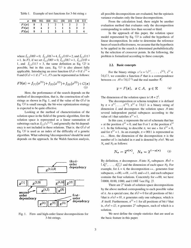
where f(2,3)(00) = 0, f(2,3)(01) = 4, f(2,3)(10) = 2, and f(2,3)(11)

= 1. In F3, if we set f(2,3)(00) = 0, f(2,3)(01) = 1, f(2,3)(10) =

1, and f(2,3)(11) = 3, the same definition as Eq. (2) is

possible, but in this case, Eq. (1) is also almost fully

applicable. Introducing an error function G(x) = 0 if x(3) =

0 and G(x) = 1 if x(3) = 1, F3 can be represented as follows:

Here, the performance of the search depends on the

method of decomposition, that is, the construction of sub-

strings as shown in Fig. 1, and if the value of the G(x) in

Eq. (3) is small enough, the bit-wise optimization strategy

is expected to be quite effective.

Looking at the method of characterization of the

solution space in the field of the genetic algorithm, first the

solution space is represented as a linear summation of

substrings such as f(2,3)(x(2,3)), and generally the bit depend-

ency is not included in these relations. That is. the G(x) of

Eq. (3) is used as an index of the difficulty of a genetic

algorithm. What substring (decomposition) should be used

depends on the approach. In the Walsh function analysis,

all possible decompositions are evaluated, but the epistasis

variance evaluates only the linear decompositions.

From the calculation load, there might be another

evaluation method that evaluates only the decomposition

corresponding to orders less than second or third.

In the approach of this paper, the solution space

model represented by Eq. (3) is called the hypothesis of

linear decomposition. In order to determine the reference

bases of search effectiveness, we assume that the hypothesis

to be applied in the search is determined probabilistically

by the selection of crossover points. In the following, the

problem is formalized according to these concepts.

2.2. Basic concepts

For the binary strings x (x = (x(1), . . . , x(L)), x(i) Î

{0,1}), we consider a function F that is a correspondence

between x Î A (= {0,1}L) and the real number R :

The dimension of the solution space is |A| = 2L.

The decomposition or schema template p is defined

by p = p(1), . . . , p(L)), p(i) Î {0,1} is a binary string of

dimension L and decomposes the solution space A into

several independent partial subspaces according to the

value of i that satisfies p(i) = 1.

In this case, p represents the set of schemata that has

* at the position p(i) = 0, and has 0 or 1 at the position p(i)

= 1. In the following, to describe p, we use * for p(i) = 0,

and for p(i) = 1. As an example, p = 0011 is represented as

**.. . Here, the dimension of the decomposition p is the

number of 1s included in p and is denoted by o(p). We set

Np and Np__ as follows:

By definition, p decomposes A into Np subspaces A(p) =

{A0(p), . . . , AN-1

(p) } and the dimension of each space Np__. For

example, for L = 4, the decomposition **.. generates four

subspaces, **00, **01, **10, and **11, and each subspace

contains the four solutions. Concretely for **00, we have

{0000, 0100, 1000, and 1100} (see Fig. 2).

There are 2L kinds of solution space decompositions

by the above method corresponding to each possible value

of p. As a special case, the p(i) = 0 for all positions of bit i

(that is o(p) = 0), p generates only one subspace, which is

A itself. Furthermore, p(i) = 1 for all positions of bit i (that

is, o(p) = L), p generates 2L subspaces, each of which is a

solution.

We next define the simple statistics that are used as

the basic feature in this paper.

Table 1. Example of test functions for 3-bit string x

(3)

Fig. 1. First- and high-order linear decompositions for

3-bit strings.

(4)

(5)

3

The overall mean mA and overall variance sA2 are the

mean and variance over all solutions, defined by

A subspace of A generated by p is denoted by a Î A(p).

The evaluation value of a is defined as the average of all

the evaluation values of the solutions included in a , and is

denoted by ma :

The between variance is the variance of the evaluation

values of the subspaces A0(p), . . . , AN-1

(p) . We denote it by

sB2(p). The within variance is the average of all variances of

each solution in the group on all Ai(p). We denote it by

sW2 (p).

Definition 1. (between variance and within variance)

From Eqs. (7), (9), and (10), the following relation exists

among these variances:

Thus, we always have 0 < sB2(p), sW

2 (p) < sA2 ,

As special cases,

sB2(p) = 0 when p(i) = 0 for all i, and

sB2(p) = sA

2 when p(i) = 1 for all i.

In the following, sB2(p) is called the variance coefficient of

the decomposition p.

2.3. Linear decomposition hypothesis formula

Consider the set P = {p1, . . . , pl} (1 < l < L),

o(pi) > 1 of one or more decompositions, satisfying the

condition,

For all bit positions k, only one decomposition has the value

pi(k) = 1, and {p1, . . . , pi} are orthogonal to each other.

When the solution x is given, x is included in one of

the subspaces A(pi) generated by the pi. This subspace is

denoted by x(pi). For example, for P = {p1, p2}, we have p1

= ..**, p2 = **.., and when x = 1001, for p1 , x(p

i) = 10**,

and for p2, x(p

2) = **01. Here, the LDH (Linear Decompo-

sition Hypothesis) is defined by using P as follows:

Definition 2. (formula of linear decomposition hy-

pothesis)

In Eq. (13), c and f(pi) are defined by

That is, Eq. (13) means assuming l long substrings

(2k1, . . . , 2kl) instead of L bits as the elements of x, and

F(x) is approximated as the linear summation of partial

evaluation functions for these l substrings. G(x) corre-

sponds to the errors of the above linear approximation, and

the strength of mutual dependency among l substrings:

Fig. 2. Decomposition of the solution space.

(6)

(7)

(8)

(9)

(10)

(11)

(12)

(13)

(14)

(15)

"

"

4

Averaged over the entire solution space, the expected

values of the second and the third terms are as follows:

2.4. Validity standards for the linear

decomposition hypothesis

Many linear decompositions are expressed by Eq.

(13), depending on the selection of the decomposition set

P. In this paper, each selection of P corresponds to a

different hypothesis about the construction of the solution

space. According to this assumption, the subspaces gener-

ated by the p1, . . . , pl are mutually independent, but the

structure in each subspace is unknown. Then for the search

strategy, we apply an independent random search for each

of the l subspaces, and combine the best solutions.

In this case, the evaluation standard for the validity

of a linear decomposition hypothesis is defined in terms of

the relative contributions of the linear components in the

evaluation. This corresponds to the coefficients of determi-

nation in the regression analysis and, from the second term

of Eq. (13), is given by:

Definition 3. (validity standard of linear decompo-

sitions)

By definition, 0 < cod(P) < 1.

If no dependent relations exist among x(p1), . . . , x(p

l),

then G(x) = 0. In particular, for P = {p*, p__

*} with o(p*) =

L, and o(p__

*) = 0, f(p)(x(p

*

)) is equivalent to F(x) itself, and

G(x) = 0. This means that the evaluation function F is

unknown and is equivalent to an extensive search of all

possible solutions.

3. Relations to Existing Solution Space

Characterization Methods

3.1. Walsh function analysis

Let �G� be the order relation between the two strings

of binary numbers. That is, if pi G pj, then o(pi) < o(pj), and

if pi(k) = 1, then pj

(k) = 1. By connecting pairs of nearby order

relations, a Hasse diagram representation of the decompo-

sitions is obtained, as illustrated in Fig. 3.

For a string of length L, a total of 2L nodes and L2L

links exist. The level of the graph corresponds to the order

of p, and the nodes at level k have k links to the upper level

and (L - k) links to the lower level. All nodes have links to

2(l-k) higher nodes and 2k lower nodes. Denoting the Walsh

function in terms of the Paley order by fi [2, 4], the Walsh

coefficients wi (i = 0, . . . , 2L � 1) are

By definition, w0 is the average of the evaluation values of

all strings contained in A:

By applying the Parseval equality,

an important relation between the Walsh coefficients and

the variance coefficient sB2(p) defined in section 2 is intro-

duced.

(16)

(17)

(18)

(19)

(20)

(21)

Fig. 3. Hasse diagram expression of decompositions.

(22)

(23)

(24)

"

5

Relation 1. (relation between Walsh coefficients

and variance coefficients)

Figure 4 shows Relation 1 expressed as a Hasse

diagram. In this figure, L = 4, and each node in the Hasse

diagram corresponds to a decomposition p, and the Walsh

coefficients wi with the same index i of p. As shown by the

figure, the variance coefficient of the decomposition p = . . .*

is the squared sum of the Walsh coefficients of lower rank.

The reason that w02 is special here is that w0 is the average

of all solutions, as shown by Eq. (23), and the variance

coefficient is calculated as the difference from this average

value.

In the above example, the variance coefficient sB2(...*)

is the sum of the degrees of dependency among the bits {1},

{2}, {3}, {1,2}, {2,3}, {3,1}, and {1, 2, 3}. Thus, while the

Walsh coefficients evaluate the individual dependencies

among bits independently, the variance coefficients by

Definition 1 are the sum of the dependencies included in

the string under consideration. The same relation as Eq. (25)

is shown as Eq. (3.11) in Ref. 8.

3.2. Epistasis variance

For the calculation of the epistasis variance, it is

sufficient to consider only one linear decomposition hy-

pothesis that consists of the L independent unit vectors

u1, . . . , uL (if k = i, then ui(k) = 1, and if k ¹ i, then ui

(k) = 0).

The linear decomposition hypothesis of Eq. (13) will then

be

In the defining formula of Ref. 5, by replacing v(S)

with F(x), Ei(a) with f(ui)(x

(ui)) and V with mA, we obtain the

epistasis variance in the form,

The epistasis variance calculates the contribution of

each bit to the entire evaluation and can be expressed by

using the linear decomposition or the primary (first-order)

Walsh coefficients. The same relation between the Walsh

coefficients and the epistasis variance is also derived as

Theorems 1 and 2 of Ref. 9.

3.3. Correlation analysis between generations

The correlation between generations for a given ge-

netic operator op is given by

where P and C are random variables representing the vari-

ance of the distribution of the evaluation values for the

parents and children, s(P) and s(C) are the standard devia-

tions of P and C, respectively, and Cov(P, C) is the covari-

ance.

We assume that the genetic operator is reflexive. That

is, that the statistical distributions of the evaluation values

for parents and children are the same. If we assume that the

selection of the parent is perfectly random,

s(P) = s(C) = sA2 . If we further assume that the selection of

the value of each bit is random (linkage equilibrium), then

E[F(pi)(x

(pi)F(pj

)(x(pj))] = 0.

Under the above assumptions, when the genetic op-

erator is applied to the parent 1, 2, . . . , and the combination

of bits transmitted to a child from parents is represented by

the decomposition pi, then the following simple relation is

introduced. If P = {p1, p2, . . . } is the linear decomposition

hypothesis:

(25)

Fig. 4. Correspondence between variance coefficients

and Walsh coefficients.

(26)

(27)

(28)

(29)

"

"

"

6

Further, assuming that prob(P) is the probability that

the given genetic operation selects the decomposition set

P, we obtain

4. Comparisons of Uniform Crossover and

One-Point Crossover

We now introduce the theory of correlation between

generations on two typical crossover operators: uniform

crossover and one-point crossover. Since the number of

parents of these crossover operators is two, it is sufficient

to consider the set of complementary decompositions P =

{p, p__

}.

4.1. Uniform crossover

In uniform crossover, each bit is selected from either

parent with the probability 1/2 to generate a new child. The

number of ways to select p is 2L, and each has the same

probability 1/(2L). Taking the average over the entire set of

the possible decompositions (p, p__

), the correlation between

generations is given by the following relation:

Relation 3. (correlation between generations in

uniform crossover).

where o(i) is the number of 1s included in the binary

expression of i. Relation 3 is also given in Ref. 10, and by

taking the correspondence of the genetic variance decom-

position to the covariance coefficient of this paper, and of

heritability to the correlation between generations, a mathe-

matically equivalent formula can be obtained. However, in

Ref. 10, additional conditions are imposed based on popu-

lation genetics and the value of each bit x(i) is not restricted

to binary numbers, where the generation probability of each

value of x(i) is considered in the random sampling. Also,

from a practical point of view, Ref. 10 employs an approxi-

mation method in which only the lower-order Walsh coef-

ficients are taken into account, but this is applicable to our

present results also.

4.2. One-point crossover

In one-point crossover, the crossover point k is se-

lected randomly (1 < k < L) and the child receives either

x(i) (i < k) or x(j) (j > k) from one parent and the rest from

the other parent. Using this rule, there are 2L ways to select

p and each has the same probability 1/(2L). Let A1p be the

2L possible decompositions of set P = (p, p__

as shown in

Fig. 5); the correlation between generations of one-point

crossover is then given by the following relation:

Relation 4. (correlation between generations in

one-point crossover)

4.3. Comparisons and discussions

Uniform crossover selects all linear decomposition

hypotheses with equal probability and is robust as a search

method. On the other hand, one-point crossover takes a

weighed selection of the linear decomposition; thus if we

can use suitable coding method, it can use the inner struc-

ture of the solution space more efficiently.

In the above analysis, both for uniform crossover and

for one-point crossover, the value of prob(Pi) is selected

equally after all possible decompositions are listed and the

correlations are calculated. Conversely, if the set P of all

possible decompositions is taken as the probability space,

and if we define the probability on P as prob(Pi) (Pi Î P,

Si prob(Pi) = 1), then prob(Pi) is the general definition of

the crossover operator and corresponds to an expression of

the domain knowledge in the genetic algorithm.

5. Experimental Results

The preconditions for the definition of the correlation

between generations in Eq. (30) no longer hold in the real

genetic algorithm, Also, we have assumed that the size of

the population is large and that the search time is long. Thus,

a simple test function is used to examine the relationships

(30)

(31)

Fig. 5. An LDH set for one-point crossover operator

when L = 5.

(32)

"

"

7

between the calculated values of the correlation between

generations and the performance of the actual genetic algo-

rithm.

5.1. Definition of the test function

In the experiments, the following four test functions

were used: EQ-IND, 4-DPND(1,5), 4-DPND(3,7), and

RANDOM. To simplify the analysis, in all functions, L =

8, that is, the dimension of the solution space was 28 = 256.

EQ-IND consisted of eight independent bits of equal

weight and the evaluation value was the number of 1s in the

strings. 4-DPND(1,5) consisted of two substrings of four

bits that occupied positions 1, 2, 3, 4 and 5, 6, 7, 8; the

evaluation value was given by the sum of the pre-set real

values for the two four-bit substrings. 4-DPND(3,7) con-

sisted of two four-bit substrings occupying positions 1, 2,

7, 8 and 3, 4, 5, 6. The evaluation value of each substring

was the same as for the case 4-DPND(1,5). RANDOM was

an evaluation function that assigns a random value between

0 and 1 for each of 28 strings.

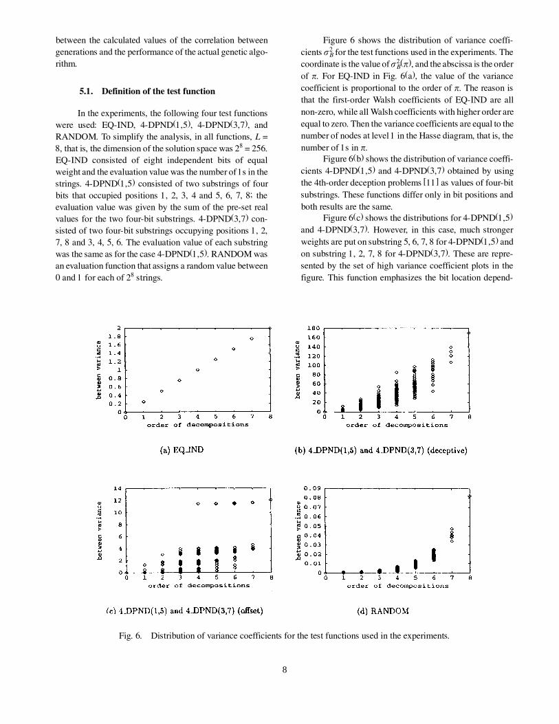
Figure 6 shows the distribution of variance coeffi-

cients sB2 for the test functions used in the experiments. The

coordinate is the value of sB2(p), and the abscissa is the order

of p. For EQ-IND in Fig. 6(a), the value of the variance

coefficient is proportional to the order of p. The reason is

that the first-order Walsh coefficients of EQ-IND are all

non-zero, while all Walsh coefficients with higher order are

equal to zero. Then the variance coefficients are equal to the

number of nodes at level 1 in the Hasse diagram, that is, the

number of 1s in p.

Figure 6(b) shows the distribution of variance coeffi-

cients 4-DPND(1,5) and 4-DPND(3,7) obtained by using

the 4th-order deception problems [11] as values of four-bit

substrings. These functions differ only in bit positions and

both results are the same.

Figure 6(c) shows the distributions for 4-DPND(1,5)

and 4-DPND(3,7). However, in this case, much stronger

weights are put on substring 5, 6, 7, 8 for 4-DPND(1,5) and

on substring 1, 2, 7, 8 for 4-DPND(3,7). These are repre-

sented by the set of high variance coefficient plots in the

figure. This function emphasizes the bit location depend-

Fig. 6. Distribution of variance coefficients for the test functions used in the experiments.

8

encies and is used to examine the differences of the one-

point crossover between 4-DPND(1,5) and 4-DPND(3,7).

Figure 6(d) shows the result obtained for RANDOM.

The Walsh coefficients are distributed uniformly and ran-

domly, and the value of the variance coefficient is propor-

tional to the total number of nodes with lower order that is

2o(p) - 1.

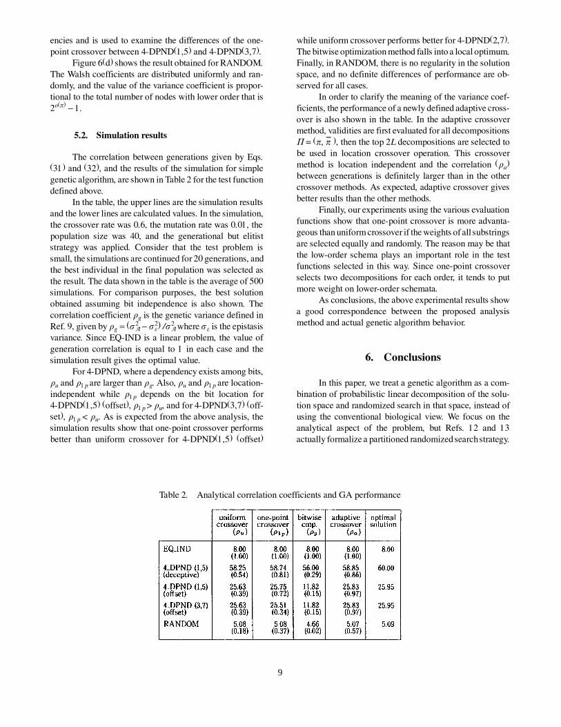
5.2. Simulation results

The correlation between generations given by Eqs.

(31) and (32), and the results of the simulation for simple

genetic algorithm, are shown in Table 2 for the test function

defined above.

In the table, the upper lines are the simulation results

and the lower lines are calculated values. In the simulation,

the crossover rate was 0.6, the mutation rate was 0.01, the

population size was 40, and the generational but elitist

strategy was applied. Consider that the test problem is

small, the simulations are continued for 20 generations, and

the best individual in the final population was selected as

the result. The data shown in the table is the average of 500

simulations. For comparison purposes, the best solution

obtained assuming bit independence is also shown. The

correlation coefficient rg is the genetic variance defined in

Ref. 9, given by rg = (sA2 - se

2) /sA2 where se is the epistasis

variance. Since EQ-IND is a linear problem, the value of

generation correlation is equal to 1 in each case and the

simulation result gives the optimal value.

For 4-DPND, where a dependency exists among bits,

ru and r1p are larger than rg. Also, ru and r1p are location-

independent while r1p depends on the bit location for

4-DPND(1,5) (offset), r1p > ru, and for 4-DPND(3,7) (off-

set), r1p < ru. As is expected from the above analysis, the

simulation results show that one-point crossover performs

better than uniform crossover for 4-DPND(1,5) (offset)

while uniform crossover performs better for 4-DPND(2,7).

The bitwise optimization method falls into a local optimum.

Finally, in RANDOM, there is no regularity in the solution

space, and no definite differences of performance are ob-

served for all cases.

In order to clarify the meaning of the variance coef-

ficients, the performance of a newly defined adaptive cross-

over is also shown in the table. In the adaptive crossover

method, validities are first evaluated for all decompositions

P = (p, p__

), then the top 2L decompositions are selected to

be used in location crossover operation. This crossover

method is location independent and the correlation (ra)

between generations is definitely larger than in the other

crossover methods. As expected, adaptive crossover gives

better results than the other methods.

Finally, our experiments using the various evaluation

functions show that one-point crossover is more advanta-

geous than uniform crossover if the weights of all substrings

are selected equally and randomly. The reason may be that

the low-order schema plays an important role in the test

functions selected in this way. Since one-point crossover

selects two decompositions for each order, it tends to put

more weight on lower-order schemata.

As conclusions, the above experimental results show

a good correspondence between the proposed analysis

method and actual genetic algorithm behavior.

6. Conclusions

In this paper, we treat a genetic algorithm as a com-

bination of probabilistic linear decomposition of the solu-

tion space and randomized search in that space, instead of

using the conventional biological view. We focus on the

analytical aspect of the problem, but Refs. 12 and 13

actually formalize a partitioned randomized search strategy.

Table 2. Analytical correlation coefficients and GA performance

9

These methods employ sequential decision theory

and at each step of the search, the action for the next step is

determined so that the decision is statistically optimized.

The methods exploit past observations at the maximum, but

the amount of data management and calculation is large and

the method itself becomes complex.

According to the viewpoint of this paper, genetic

algorithms avoid such complex calculations, but select the

next search action (linear decomposition hypothesis) with

a certain pre-determined probability. The efficiency of the

search inevitably depends on the coding method and the

design of genetic operators, but the strategy itself becomes

simple.

REFERENCES

1. A.D. Bethke. Genetic Algorithms as Function Op-

timizers. Doctorial Dissertation, University of Michi-

gan (1981).

2. D.E. Goldberg. Genetic algorithms and Walsh func-

tions: Part I, a gentle introduction. Complex Systems,

3, pp. 129�152 (1989).

3. D.E. Goldberg. Genetic algorithms and Walsh func-

tions: Part II, deception and its analysis. Complex

Systems, 3, pp. 153�171 (1989).

4. Y. Endo. Walsh Analysis. Tokyo Denkidaigaku Publ.

(1993). (in Japanese)

5. Y. Davidor. Epistasis variance: A viewpoint on GA-

hardness. Foundations of Genetic Algorithms, pp.

23�35 (1991).

6. B. Manderic, M. DeWeger, and P. Spiessens. The

genetic algorithm and the structure of the fitness

landscape. Proceedings of the 4th International Con-

ference on Genetic Algorithms, pp. 143�150 (1991).

7. A. Aizawa. Fitness landscape characterization by

variance of decompositions. Foundation of Genetic

Algorithms 4, eds., R.K. Belew and M.D. Vose, pp.

225�245 (1997).

8. M. Rudnic and D.E. Goldberg. Signal, noise, and

genetic algorithms. IlliGAL Report, No. 91005

(1991).

9. M. Manela and J.A. Campbell. Harmonic analysis,

epistasis and genetic algorithms. Parallel Problem

Solving from Nature 2, eds., R. Männer and B. Man-

derick. Elsevier Science Publishers, pp. 57�64

(1992).

10. H. Asoh and H. Mühlenbein. Estimating the herita-

bility by decomposing the genetic variance. Parallel

Problem Solving from Nature, 3, eds., Y. Davidor,

H.P. Schwefel, and R. Männer. Elsevier Science Pub-

lishers, pp. 98�107 (1994).

11. L.D. Whitley. Fundamental principles of deception in

genetic search. Foundations of Genetic Algorithms,

ed., G.J.E. Rawlins. Morgan Kaufmann Publisher,

pp. 221�241 (1991).

12. Z.B. Tang. Adaptive partitioned random search to

global optimization. IEEE Transactions on Automat-

ic Control, 39, No. 11, pp. 2235�2244 (Nov. 1994).

13. C.C. Peck and A.P. Dhawan. Genetic algorithms as

global random search methods: An alternative per-

spective. Evolutionary Computation, 3, No. 1, pp.

39�80 (1995).

AUTHOR

Akiko Aizawa (member) received her B.Eng. and D.Eng. degrees from the University of Tokyo in 1985 and 1990. She

was a Visiting Scholar at University of Illinois from 1990�1992. She is now an associate professor at the National Center for

Information Systems. Research on knowledge engineering and communication network engineering.

10