Embed Size (px)
Citation preview
Genetic Algorithms and Neural Networks: A Comparison Basedon the Repeated Prisoner’s Dilemma
Robert E. Marks,1
AGSM, UNSW, Sydney, NSW [email protected]
Hermann Schnabl,University of Stuttgart and AGSM, UNSW
Revised: May 15, 1998.
ABSTRACT Genetic Algorithms (GAs) and Neural Networks (NNs) in a widesense both belong to the class of evolutionary computing algorithms that tryto mimic natural evolution or information handling with respect to everydayproblems such as forecasting the stock market, firms’ turnovers, or theidentification of credit bonus classes for banks. Both methods have gainedmore ground in recent years, especially with respect to micro-economicquestions. But owing to the dynamics inherent in their evolution, they belongto somewhat disjunct development communities that interact seldom. Hencecomparisons between the different methods are rare. Despite their obviousdesign differences, they also have several features in common that aresufficiently interesting for the innovation-oriented to follow up and so tounderstand these commonalities and differences. This paper is anintroductory demonstration of how these two methodologies tackle the well-known Repeated Prisoner’s Dilemma.
_______________1. The first author wishes to acknowledge the support of the Australian Research Council.
- 1 -

1. Introduction
The relationship between biology and economics has been long: it is said that150 years ago both Wallace and Darwin were influenced by Malthus’ writingson the rising pressures on people in a world in which human populationnumbers grew geometrically while food production only grew arithmetically.In the early 1950s there was an awakening that the processes of marketcompetition in a sense mimicked those of natural selection. This thread hasfollowed through to the present, in an “evolutionary” approach to industrialorganisation. Recently, however, computer scientists and economists havebegun to apply principles borrowed from biology to a variety of complexproblems in optimisation and in modelling the adaptation and change thatoccurs in real-world markets. There are three main techniques: ArtificialNeural Networks, Evolutionary Algorithms (EAs), and Artificial Economies,related to Artificial Life. Neural nets are described below. We discussEvolutionary Algorithms2 in general, and Genetic Algorithms in particular,below.3
Techniques of artificial economies borrow from the emerging disciplineof artificial life (Langton et al. 1992) to examine through computer simulationconditions sufficient for specific economic macro-phenomena to emerge fromthe interaction of micro units, that is, economic agents. Indeed, EvolutionaryAlgorithms may be seen as falling into the general area of the study ofcomplexity. In our view, the emergence of such objects of interest ascharacteristics, attributes, or behaviour distinguishes complexity studies fromtraditional deduction or induction. Macro phenomena emerge in sometimesunexpected fashion from aggregation of interaction of micro units, whoseindividual behaviour is well understood.
Genetic Algorithms (GAs) and Neural Networks (NNs) in a wide senseboth belong to the class of evolutionary computing algorithms that try tomimic natural evolution or information handling with respect to everydayproblems such as forecasting the stock market, firms’ turnovers, or theidentification of credit bonus classes for banks.4 Both methods have gained
_______________2. Examples of EAs are: Genetic Algorithms (GAs), Genetic Programming (GP), Evolutionary
Strategies (ESs), and Evolutionary Programming (EP). GP (Koza 1992) was developedfrom GAs, and EP (Sebald & Fogel 1994) from ESs, but GAs and ESs developedindependently, a case of convergent evolution of ideas. ESs were devised by Germanresearchers in the 1960s (Rechenberg 1973, Schwefel & Manner 1991), and GAs weresuggested by John Holland in 1975. Earlier, Larry Fogel and others had developed analgorithm which relied more on mutation than on the sharing of information betweengood trial solutions, analogous to “crossover” of genetic material, thus giving rise to so-called EP.
3. In his Chapter 4, Networks and artificial intelligence, Sargent (1993) outlines NeuralNetworks, Genetic Algorithms, and Classifier Systems. Of interest, he remarks on theparallels between neural networks and econometrics in terms of problems and methods,following White (1992).
4. Commonalities between both methods are: mimicking events/behaviour as informationflows within a learned or adaptive structure. Differences among EAs include: theirmethods of solution representation, the sequence of their operations, their selectionschemes, how crossover/mutation are used, and the determination of their strategyparameters
- 2 -

more ground in recent years, especially with respect to micro-economicquestions. Despite their obvious design differences, they also have severalfeatures in common that are sufficiently interesting for the innovation-oriented to follow up and so to understand these commonalities anddifferences.5 Owing to the dynamics inherent in the evolution of bothmethodologies, they belong to somewhat disjunct scientific communities thatinteract seldom. Therefore, comparisons between the different methods arerare.
Genetic Algorithms (GAs) essentially started with the work of Holland(1975), who in effect tried to use Nature’s genetically based evolutionaryprocess to effectively investigate unknown search spaces for optimalsolutions. The DNA of the biological genotype is mimicked by a bit string.Each bit string is seeded randomly for the starting phase and then goesthrough various (and also varying) procedures of mutation, mating afterdifferent rules, crossover, sometimes also inversion and other “changingdevices” very similar to its biological origins in Genetics. A fitness functionworks as a selection engine that supervises the whole simulated evolutionwithin the population of these genes, and thus drives the process towardssome optimum, measured by the fitness function. Introductory Section 2gives more details on GAs and their potential in solving economic problems.
Neural Networks (NNs) are based on early work of McCulloch & Pitts(1943), who built a first crude model of a biological neuron with the aim tosimulate essential traits of biological information handling. In principle, aneuron gathers information about the environment via synaptic inputs on itsso-called dendrites (= input channels) — which may stem from sensory cellssuch as in the ear or eye) or from other neurons — compares this input to agiven threshold value, and, under certain conditions, “fires” its axon (= outputchannel), which leads to an output to a muscle cell or to another neuron thattakes it as information input again. Thus, a neuron can be viewed as acomplex “IF...THEN...[ELSE]...” switch. Translated into an economic context,the neural mechanism mimics decision making rules such as “IF the interestrate falls AND the inflation rate is still low THEN engage in new buys on thestock market,” where the capital letters reflect the switching mechanisminherent in the neural mechanism. Still more realistic state-of-the-artmodelling replaces the implicit assumption of weights of unity (for thestraight “IF” resp. the “AND”) by real-valued weights. Thus, the aboveIF..THEN example turns into more fuzzy information handling, viz.: “IF(with probability 0.7) the interest rate is lowered AND (with probability 0.8)the inflation rate is still low THEN engage in new buys on the stock market”.This fuzzier approach also reflects different strengths of synaptic impact in
_______________5. This paper aims to be an introductory demonstration of how these two methodologies
tackle the well-known Repeated Prisoner’s Dilemma. A further paper may concentrate onboth methods’ basic approaches in handling the given information in achieving theirgoals.
- 3 -

the biological paradigm.While a single neuron is already a pretty complex “switch”, it is clear
that a system of many neurons, a neural network, comprising certaincombinations of units, mostly in patterns of hierarchical layers, will be able tohandle even more complex tasks.
Development of the NN approach to solving everyday problems madegood progress until the late ’sixties, but withered after an annihilatingcritique by Minsky & Papert (1967). This attack was aimed at the so-called“linear separability problem” inherent in 2-layer models, but was taken asbeing true for all NN models. The problem inherent in the criticised modelswas that a Multi-Layer-Perceptron (MLP), which could handle non-linearproblems, lacked an efficient learning algorithm and thus was not applicablein practice. The cure came with the publication of Rumelhart & McClelland(1986) on the solution of the so-called (Error-) Backpropagation Algorithmthat made nonlinear NNs workable.
The name “Neural Networks” already describes what they try to do, i.e.to handle information like biological neurons do, and thus using theaccumulated experience of nature or evolution in developing those obviouslyeffective and viable tools for real-time prediction tasks. (One thinks ofplaying tennis and the necessary on-line forecast of where the ball will be sothe player can return it.) There is also a growing list of successful economicapplications, including forecasting stock markets and options and creditbonus assignments, as well as more technically oriented tasks with economicimplications, such as detecting bombs in luggage, detecting approachingairplanes including their brand type by classifying radar signals, ordiagnosing diseases from their symptoms. Section 2 is an introduction toGAs. Section 3 is an introduction to NNs. Sections 4 and 5 then show howthe Repeated Prisoner’s Dilemma (RPD) is tackled by each method.
2. The Genetic Algorithm Approach — A Short Introduction
Genetic algorithms are a specific form of EA. The standard GA can becharacterised by: operating on a population of bit-strings (0 or 1). whereeach string represents a solution, and GA individual strings are characterisedby a duality of: the structure of the bit-string (the genotype), and theperformance of the bit-string (the phenotype).6 In general the phenotype (thestring’s performance) emerges from the genotype.
_______________6. We characterise the phenotype as the performance or behaviour when following the now-
standard approach of using GAs in studying game-playing, in particular playing theRepeated Prisoner’s Dilemma, since the only characteristic of concern is the individual’sperformance in the repeated game. Such performance is entirely determined by thestring’s structure, or genotype, as well, of course, by the rival’s previous behaviour.
- 4 -

2.1 GA: The evolutionary elements:
There are four evolutionary elements:7
1. Selection of parent individuals or strings can be achieved by a “wheel offortune” process, where a string’s probability of selection is proportionalto its performance against the total performance of all strings.
2. Crossover takes pairs of mating partners, and exchanges segmentsbetween the two, based on a randomly chosen common crossover pointalong both strings.
3. Mutation: with a small probability each bit is flipped. This eliminatespremature convergence on a sub-optimal solution by introducing new bitvalues into a population of solutions.
4. Encoding is the way in which the artificial agent’s contingent behaviouris mapped from the individual’s structure to its behaviour. As well asthe decision of whether to use binary or decimal digits, or perhapsfloating-point numbers, there is also the way in which the model isencoded.
2.2 Detailed description of a GA8
How can we use the GA to code for the behaviour of the artificial adaptiveagents? How can strategies (sets of rules) for playing repeated games of theRepeated Prisoner’s Dilemma (RPD) be represented as bit strings of zeroesand ones, each locus or substring (or gene) along the string mapping uniquelyfrom a contingent state — defined by all players’ moves in the previous roundor rounds of the repeated game — to a move in the next round, or a means ofdetermining this next move? This coding problem is discussed in more detailbelow.
We describe these behaviour-encoding strings as “chromosomes”because, in order to generate new sets of strings (a new generation of“offspring”) from the previous set of strings, GAs use selection andrecombinant operators — crossover and mutation — derived by analogy frompopulation genetics. Brady (1985) notes that “during the course of evolution,slowly evolving genes would have been overtaken by genes with betterevolutionary strategies,” although there is some dispute about the extent towhich such outcomes are optimal (Dupre 1987). The GA can be thought of asan optimization method which overcomes the problem of local fitness optima,to obtain optima which are almost always close to global (Bethke 1981).
_______________7. There are variants for each of these. Selection: linear dynamic scaling, linear ranking,
stochastic universal sampling, survival of elites. Crossover: n-point crossover, uniformcrossover. Coding: Gray code — small genotype changes → small phenotype changes;decimal strings; real numbers.
8. For an introduction to GAs, see Goldberg (1989). See also Davis (1991), Michalewicz(1994), Nissen & Biethahn (1995), and Mitchell (1996).
- 5 -
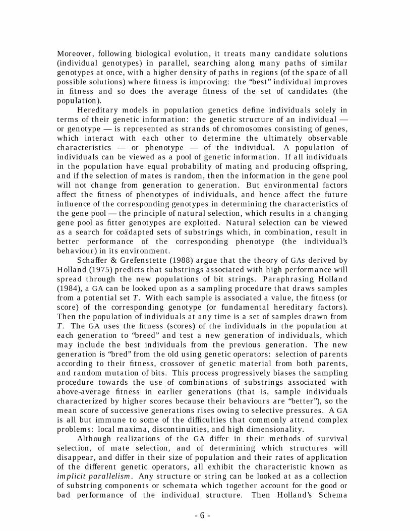
Moreover, following biological evolution, it treats many candidate solutions(individual genotypes) in parallel, searching along many paths of similargenotypes at once, with a higher density of paths in regions (of the space of allpossible solutions) where fitness is improving: the “best” individual improvesin fitness and so does the average fitness of the set of candidates (thepopulation).
Hereditary models in population genetics define individuals solely interms of their genetic information: the genetic structure of an individual —or genotype — is represented as strands of chromosomes consisting of genes,which interact with each other to determine the ultimately observablecharacteristics — or phenotype — of the individual. A population ofindividuals can be viewed as a pool of genetic information. If all individualsin the population have equal probability of mating and producing offspring,and if the selection of mates is random, then the information in the gene poolwill not change from generation to generation. But environmental factorsaffect the fitness of phenotypes of individuals, and hence affect the futureinfluence of the corresponding genotypes in determining the characteristics ofthe gene pool — the principle of natural selection, which results in a changinggene pool as fitter genotypes are exploited. Natural selection can be viewedas a search for coadapted sets of substrings which, in combination, result inbetter performance of the corresponding phenotype (the individual’sbehaviour) in its environment.
Schaffer & Grefenstette (1988) argue that the theory of GAs derived byHolland (1975) predicts that substrings associated with high performance willspread through the new populations of bit strings. Paraphrasing Holland(1984), a GA can be looked upon as a sampling procedure that draws samplesfrom a potential set T. With each sample is associated a value, the fitness (orscore) of the corresponding genotype (or fundamental hereditary factors).Then the population of individuals at any time is a set of samples drawn fromT. The GA uses the fitness (scores) of the individuals in the population ateach generation to “breed” and test a new generation of individuals, whichmay include the best individuals from the previous generation. The newgeneration is “bred” from the old using genetic operators: selection of parentsaccording to their fitness, crossover of genetic material from both parents,and random mutation of bits. This process progressively biases the samplingprocedure towards the use of combinations of substrings associated withabove-average fitness in earlier generations (that is, sample individualscharacterized by higher scores because their behaviours are “better”), so themean score of successive generations rises owing to selective pressures. A GAis all but immune to some of the difficulties that commonly attend complexproblems: local maxima, discontinuities, and high dimensionality.
Although realizations of the GA differ in their methods of survivalselection, of mate selection, and of determining which structures willdisappear, and differ in their size of population and their rates of applicationof the different genetic operators, all exhibit the characteristic known asimplicit parallelism. Any structure or string can be looked at as a collectionof substring components or schemata which together account for the good orbad performance of the individual structure. Then Holland’s Schema
- 6 -
Sampling Theorem (Holland 1975, Mitchell 1996) demonstrates thatschemata represented in the population will be sampled in future generationsin relation to their observed average fitness, if we can assume that theaverage fitness of a schema may be estimated by observing some of itsmembers. (Note that many more schemata are being sampled than areindividual structures of the population being evaluated.) Genetic algorithmsgain their power by exploring the space of all schemata and by quicklyidentifying and exploiting the combinations which are associated with highperformance.
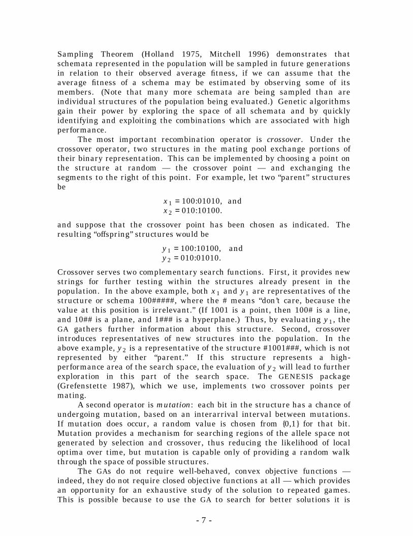
The most important recombination operator is crossover. Under thecrossover operator, two structures in the mating pool exchange portions oftheir binary representation. This can be implemented by choosing a point onthe structure at random — the crossover point — and exchanging thesegments to the right of this point. For example, let two “parent” structuresbe
x 1 = 100:01010, andx 2 = 010:10100.
and suppose that the crossover point has been chosen as indicated. Theresulting “offspring” structures would be
y 1 = 100:10100, andy 2 = 010:01010.
Crossover serves two complementary search functions. First, it provides newstrings for further testing within the structures already present in thepopulation. In the above example, both x 1 and y 1 are representatives of thestructure or schema 100#####, where the # means “don’t care, because thevalue at this position is irrelevant.” (If 1001 is a point, then 100# is a line,and 10## is a plane, and 1### is a hyperplane.) Thus, by evaluating y 1, theGA gathers further information about this structure. Second, crossoverintroduces representatives of new structures into the population. In theabove example, y 2 is a representative of the structure #1001###, which is notrepresented by either “parent.” If this structure represents a high-performance area of the search space, the evaluation of y 2 will lead to furtherexploration in this part of the search space. The GENESIS package(Grefenstette 1987), which we use, implements two crossover points permating.
A second operator is mutation: each bit in the structure has a chance ofundergoing mutation, based on an interarrival interval between mutations.If mutation does occur, a random value is chosen from {0,1} for that bit.Mutation provides a mechanism for searching regions of the allele space notgenerated by selection and crossover, thus reducing the likelihood of localoptima over time, but mutation is capable only of providing a random walkthrough the space of possible structures.
The GAs do not require well-behaved, convex objective functions —indeed, they do not require closed objective functions at all — which providesan opportunity for an exhaustive study of the solution to repeated games.This is possible because to use the GA to search for better solutions it is
- 7 -

sufficient that each individual solution can be scored for its “evolutionaryfitness:” in our case the aggregate score of a repeated game provides thatmeasure, but in general any value that depends on the particular pattern ofeach individual chromosome will do.
2.3 Applications
For a comprehensive survey of the use of evolutionary algorithms, and GAs inparticular, in management applications, see Nissen (1995). In Industry:production planning, operations scheduling, personnel scheduling, linebalancing, grouping orders, sequencing, and siting. In financial services:risks assessment and management, developing dealing rules, modellingtrading behaviour, portfolio selection and optimisation, credit scoring, andtime series analysis.
3. The Neural Network Approach — A Short Introduction
Neural Nets9 can be classified in a systematic way as systems or modelscomposed of “nodes” and “arcs”, where the nodes are artificial neurons orunits (in order to distinguish them from their biological counterparts, whichthey mimic only with respect to the most basic features). Usually, within aspecific NN all units are the same. The arcs, or connections between theunits, simultaneously mimic the biological axons and the dendrites (inbiology, the fan-in or input-gathering devices) including the synapses (i.e. theinformation interface between the firing axon and the information-takingdendrite). Their artificial counterpart is just a “weight” (given by a real-valued number) that reflects the strength of a given “synaptic” connection.The type of connectivity, however, is the basis for huge diversity in NNarchitectures, which accompanies great diversity in their behaviour. Figure 1shows the described relationships between the biological neuron and itsartificial counterpart, the unit.
3.1 Units and Neurons
There are two functions governing the behaviour of a unit, which normallyare the same for all units within the whole NN, i.e.
• the input function, and• the output function.
The input function is normally given by equation (1). The unit underconsideration, unit j, integrates or sums up the numerous inputs:
netj =iΣwijxi , (1)
where netj describes the result of the net inputs xi (weighted by the weightswij) impacting on unit j (cf. the arrows in Figure 1, lower graph). Theseinputs can stem from two sources. First, if unit j belongs to the hierarchically
- 8 -


Figure 1. Neuron and Unit
lowest layer of the NN — the input layer — then they are caused by theenvironment. Second, if unit j belongs to a hierarchically higher layer of theNN, such as the hidden layer or the output layer, then the inputs come fromunits below unit j in the hierarchy. (In Figures 3 and 4, below, this meansfrom units on the left.) Thus, in vector notation, the input function (1) sumsthe inputs xi of its input vector x according to their “strengths”, using theappropriate weights of a weight matrix W = {wij}.
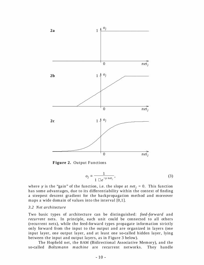
The output function exhibits a great variety, and has the biggest impacton behaviour and performance of the NN. The main task of the outputfunction is to map the outlying values of the obtained neural input back to abounded interval such as [0,1] or [–1,+1].10 Figure 2 shows some of the mostfrequently used output functions, oj = f (netj) = f (
iΣ wij xi).
The output oj for a digital (or Heaviside) function would, for example, begiven by equation (2) (Figure 2a):
oj = D (netj − T) = D (iΣwij xi − T), (2)
where the symbol D stands for the Dirichlet operator, which gives a “stepfunction”. Given, for example, a threshold T = 0.5, then output oj = 1 if netj >0.5, and oj = 0 otherwise. (See also Figure 2a, but for T = 0.) Other functionsare the semi-linear function (see Figure 2b), and the so-called Fermi orsigmoid functions (Figure 2c and equation (3)):
_______________9. For a rigorous introduction, see White (1992) or Bertsekas & Tsitsiklis (1996).10. For this reason, the output function is sometimes known as the “squasher” function
(Sargent 1993, p.54.)
- 9 -
netj
oj1
0
2a
netj
oj1
0
2b
netj
oj1
0
2c
Figure 2. Output Functions
oj =1 + e −γ netj
1__________, (3)
where γ is the “gain” of the function, i.e. the slope at netj = 0. This functionhas some advantages, due to its differentiability within the context of findinga steepest descent gradient for the backpropagation method and moreovermaps a wide domain of values into the interval [0,1].
3.2 Net architecture
Two basic types of architecture can be distinguished: feed-forward andrecurrent nets. In principle, each unit could be connected to all others(recurrent nets), while the feed-forward types propagate information strictlyonly forward from the input to the output and are organized in layers (oneinput layer, one output layer, and at least one so-called hidden layer, lyingbetween the input and output layers, as in Figure 3 below).
The Hopfield net, the BAM (Bidirectional Associative Memory), and theso-called Boltzmann machine are recurrent networks. They handle
- 10 -

nonlinearities very well, but have a very limited “memory”, i.e. they cangeneralize only for less differentiated cases, compared to the feed-forwardtype. It turns out that the MLP (Multi-Layer Perceptron), a standard feed-forward type of NN, is best suited to use in the economic context, because itsability to take into account complex situations is much higher than those ofthe recurrent nets. We therefore focus on this type of NN architecture here.
3.3 Learning strategies
In addition to the output function used and the net architecture, the way theylearn is a third criterion defining the structure and performance of NNs. Wedistinguish, first, supervised learning (where the “trainer” of the net knowsthe correct result and gives this information to the net with each learningstep) and, second, unsupervised learning (where the net itself has to learnwhat is correct and what is not correct, mainly by using measures ofsimilarity with events encountered earlier in the “learning history”).Moreover, the way a NN learns also depends on the structure of the NN andcannot be examined separately from its design. Therefore, we again focus onthe most common type of learning, developed for the MLP, which is ErrorBackpropagation, although we also consider its predecessors.
There is a history of learning rules which starts with the so-called Hebbrule, formulated following Donald Hebb’s observation in neurology that thesynaptic connection between two neurons is enhanced if they are active at thesame time (Hebb 1949). As learning in the NN is simulated by adapting the(information-forwarding) weights between the different layers, this leads toequation (4) for an appropriate weight adaptation:
∆wij =η oi oj , (4)
where η is an appropriate learning rate (mostly 0 < η < 1) and wij stands forthe weight connecting, for example, input unit i and a unit j, located in thehidden layer.
Further development yielded the so-called Delta rule, which is a kind of“goal-deviation correction” (Widrow & Hoff 1960). Its formula is given byequation (5):
∆wij =η ( zj − oj ) oi , (5)
where η again gives the learning rate, and where zj is the jth element of thegoal vector. Thus, δδ = z − o describes the vector of deviations between theoutput propagated by the actual weight structure of the NN and the desiredvalues of the target vector. The so-called generalized Delta rule at the heartof the Backpropagation Algorithm is given by equation (6) in a general form,for a weight matrix between any two layers, and must be further specified,when applied, with respect to the layers to which the weight matrix then iscontingent:
∆wij =η δ j oi. (6)
This specification is done in defining the error term δ j in (6), since unit j is amember of the output layer or any hidden layer. For an output unit j, theFermi output function (see Figure 2c and equation (3)) is mostly used, so that
- 11 -
the derivative is easy to calculate:
δ j = oj(1 − oj)(zj − oj). (7)
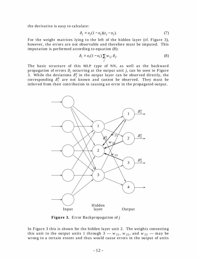
For the weight matrices lying to the left of the hidden layer (cf. Figure 3),however, the errors are not observable and therefore must be imputed. Thisimputation is performed according to equation (8):
δ i = oi(1 − oi)jΣ wij δ j . (8)
The basic structure of this MLP type of NN, as well as the backwardpropagation of errors δ j occurring at the output unit j, can be seen in Figure3. While the deviations δ j
o in the output layer can be observed directly, thecorresponding δ i
h are not known and cannot be observed. They must beinferred from their contribution in causing an error in the propagated output.
3
2
δ 2h
1
4
3
2
1
w 23
w 22
w 21
δ 3o
δ 2o
δ 1o
InputHiddenlayer Output
Figure 3. Error Backpropagation of j
In Figure 3 this is shown for the hidden layer unit 2. The weights connectingthis unit to the output units 1 through 3 — w 21, w 22, and w 23 — may bewrong to a certain extent and thus would cause errors in the output of units
- 12 -

1, 2 and 3. Correcting them in an appropriate manner, which takes intoaccount their contribution in causing the errors, is called ErrorBackpropagation, since the errors δ j are imputed in a backwards directionand the weights concerned are adjusted in a manner such that a quadraticerror function of the difference between target and NN output is minimized.
For example, the error of the hidden layer unit 2 is imputed by thecontribution of its forward-directed information to the errors in the outputlayer, which were produced by these signals. The forward-directed signals(from each unit — here, unit 2 — of the hidden layer to several units of theoutput layer — here, units 1, 2, and 3) contribute to the output errors (hereδ 1
o , δ 2o , and δ 3
o , the errors in the signals from units 1, 2, and 3 in the outputlayer, respectively). The greater the error (δ 2
h) at the hidden unit 2, thegreater the errors δ 1
o , δ 2o , and δ 3
o at the output units 1, 2, and 3, respectively.So, in order to calculate the error (δ 2
h) at hidden unit 2, we must sum theerrors observed from all output-layer units to which the hidden unit 2contributes, suitable adjusted by the three weights of the signals from hiddenunit 2 to the output layer units wij (shown in Figure 3 as linking output-layerunit j and hidden-layer unit i; see the big-headed arrows). Therefore it isimportant in using a steepest-descent mechanism that the alterations of theweights can be found by differentiating the various output functions of theappropriate units (cf. Rumelhart & McClelland 1986).
Besides the Backpropagation Algorithm, which because of its gradientmethod approach may suffer the problem of converging to local minima, thereare other methods for “learning”, i.e. adapting the weights, in the basket ofevolutionary computing including GAs and the Evolutionary Strategies, all ofwhich use a fitness function as an implicit error function. But these moreevolutionary algorithms of learning do not use backpropagation.
Using NNs for everyday problems shows that there can be a tendency fora NN to “overfit” by learning the noise contained in the data too well, whichreduces the potential for generalizing or the possibility of forecasting. Thishas led to different approaches to avoid overfitting of the weights to noise.One approach is to split the data set about 70%, 20% and 10%, using the firstset for training and the second for validation and to end learning if thereported value of the error function increases again after a longer phase ofreduction in the first part of the learning. Another approach takes intoaccount that the architecture or final structure of a NN is highly dependent onthe data. It then “prunes” the least important units and/or links of the NNbefore it continues learning data noise, and restarts learning. With the lastdata set covering 10% of the data, one can then test the “true” forecastingpotential of the net, as these data are still unknown to the NN.
4. The GA Solution to the Repeated Prisoner’s Dilemma
To apply the GA to the solution of the Repeated Prisoner’s Dilemma (RPD),each individual string can be thought of as a mapping from the previous stateof the game to an action (cooperate C or defect D) in the next round. That is,the players are modelled as stimulus-response automata, and the GA in effectsearches for automata which score well in a RPD.11 The RPD can pit each
- 13 -
individual in each population, or it can pit each individual against anenvironment of unchanging automata. The first method results inbootstrapping or coevolution of individuals, since each generation changesand so provides a changing niche for other players. The second method wasused by Axelrod and Forrest (Axelrod 1987) in the first use of the GA tosimulate the RPD — their niche of rivals was obtained by using thealgorithms — some stochastic — that had been submitted to Axelrod’s now-famous computer tournaments (Axelrod 1984). Bootstrapping was first usedby Marks (1992a), and it is this we describe here.
Choice of the environment is determined by the issue one is examining.For the RPD there is then the issue of how to model each artificial agent.12
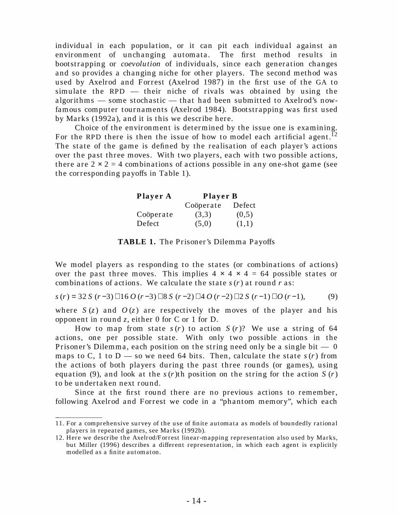
The state of the game is defined by the realisation of each player’s actionsover the past three moves. With two players, each with two possible actions,there are 2 × 2 = 4 combinations of actions possible in any one-shot game (seethe corresponding payoffs in Table 1).
Player A Player BCooperate Defect
Cooperate (3,3) (0,5)Defect (5,0) (1,1)
TABLE 1. The Prisoner’s Dilemma Payoffs
We model players as responding to the states (or combinations of actions)over the past three moves. This implies 4 × 4 × 4 = 64 possible states orcombinations of actions. We calculate the state s (r) at round r as:
s (r) = 32 S (r −3) + 16 O (r −3) + 8 S (r −2) + 4 O (r −2) + 2 S (r −1) + O (r −1), (9)
where S (z) and O (z) are respectively the moves of the player and hisopponent in round z, either 0 for C or 1 for D.
How to map from state s (r) to action S (r)? We use a string of 64actions, one per possible state. With only two possible actions in thePrisoner’s Dilemma, each position on the string need only be a single bit — 0maps to C, 1 to D — so we need 64 bits. Then, calculate the state s (r) fromthe actions of both players during the past three rounds (or games), usingequation (9), and look at the s (r)th position on the string for the action S (r)to be undertaken next round.
Since at the first round there are no previous actions to remember,following Axelrod and Forrest we code in a “phantom memory”, which each
_______________11. For a comprehensive survey of the use of finite automata as models of boundedly rational
players in repeated games, see Marks (1992b).12. Here we describe the Axelrod/Forrest linear-mapping representation also used by Marks,
but Miller (1996) describes a different representation, in which each agent is explicitlymodelled as a finite automaton.
- 14 -

agent uses during the first three rounds in order to have a state from which tomap the next action. We model this with an additional 6 bits — 2 bits perphantom round — which are used in equation (9) to establish the states andhence moves in the first three rounds; for succeeding rounds in the RPD, theactual moves are remembered and used in equation (9). For each repeatedgame, the history of play will be path-dependent, so by encoding the phantommemory as a segment of the bit string to be evolved by the GA over successivegenerations, we have effectively endogenised the initial conditions of the RPD.
Each player is thus modelled as a 70-bit string: 64 bits for the state-to-action mappings, plus 6 bits to provide the phantom memory of the threeprevious rounds’ moves at the first round. This string remains unchangedduring the RPD, and is only altered when a new population of 50 artificialagents is generated (see Step 4 below) by the GA, which uses the “genetic”operations of selection, crossover, and mutation. The first generation ofstrings are chosen randomly, which means that the mappings from state toaction are random too.
The process of artificial evolution proceeds as follows:
1. In order to determine how well it performs in playing the RPD (inevolutionary terms its “fitness”), each of the population of 50 strings ispair-wise matched against all other strings. This implies 2,500matchings, but symmetry of the payoff matrix means that only 1,275matchings are unique.13
2. Each pair-wise match consists of 22 rounds of repeated interactions,with the Prisoner’s Dilemma payoffs (see Table 1) for each interactionand each unchanging 70-bit string.14
3. Each string’s fitness is the mean of its scoring in the 1,275 22-roundencounters.
4. After all matches have occurred, a new population is generated by theGA, in which strings with a high score or fitness are more likely to beparents and so pass on some of their “genes” or fragments of their stringstructures to their offspring.
5. After several generations, the selective pressure towards those stringsthat score better means that individual strings emerge with muchhigher scores and that the population’s average performance alsorises.15
_______________13. The diagonal elements of an n × n matrix, plus half the off-diagonal elements (the upper
or lower half) number n (n +1)/2.14. As discussed in Marks (1992a), a game length of 22 corresponds to a discount factor of
0.67% per round. Note that the strings do not engage in counting (beyond three rounds)or in end-game behaviour.
15. Since there is coevolution of one’s competing players, this improvement may not be asmarked as the improvements seen when playing against an unchanging environment ofplayers, as in Axelrod (1987). A recent book by Gould (1996) discusses this issue.
- 15 -

6. The evolutionary process ends after convergence of the genotype (asmeasured by the GA) or convergence of the phenotype (as seen by thepattern of play in the RPD.
4.1 Results of the GA Approach
As mentioned above, Axelrod and Forrest (Axelrod 1987) were the first to usethe GA in simulating the RPD. Axelrod (1984) had earlier invited submissionsof algorithms for playing the RPD in two computer tournaments. Rapoport’ssimple Tit for Tat emerged as an extremely robust algorithm in bothtournaments. One can consider Axelrod’s use of the GA as a way of searchingfor new algorithms, and indeed this was explicitly done by Fujiki & Dickinson(1987), but using an early form of Genetic Programming, not a GeneticAlgorithm. Axelrod and Forrest bred their mapping strings against a fixedniche of strategies, a weighted combination of algorithms submitted to theearlier tournament.
We describe results first presented at the annual ASSA meetings in NewYork in 1988 under the auspices of the Econometric Society, and laterpublished (Marks 1992a), in which the niche — comprised of all otherindividuals in each generation — evolves as a consequence of theimprovements of the individual mappings, generation from generation. Thisis bootstrapping, or coevolution, and was also pioneered by Miller (1996).
With coevolution, the outcome of interest is emergence of convergingphenotypic characteristics, not the emergence of common genotypes. In ourexample, this means the emergence of behaviour in the RPD, not theemergence of common mappings. The main reason is that, given the selectivepressures towards mutual cooperation (CC), as reflected in the payoff matrixof Table 1, there is selective pressure against other behaviour (phenotypes),and hence against positions on the string (genes) which correspond to one ormore defections in the past three rounds.
As one would expect, mutual cooperation (CC) soon emerges as theoutcome of coevolution of mapping strings, although high rates of mutationmay occasionally disrupt this for some time.
5. The NN Solution to the Repeated Prisoner’s Dilemma
The RPD can also be tackled by a NN. As with the GA solution, we assumethree rounds back of “memory”, i.e. the players take into account their ownlast three moves as well as the last three moves of their opponent in order toreach their own decision. As the decision encompasses only two possiblemoves — to cooperate or to defect — we can translate it to +1 (cooperate) or–1 (defect) as the only output of the NN. Thus, the input layer and the outputlayer are fixed, due to the specificity of the task, and only the hidden layer(besides the weights) offers a chance of adaptation towards an optimum.
This network structure is shown in Figure 4 and was taken from Fogel& Harrald (1994), whose experiments with this type of NN we follow here.16
- 16 -

Self (t −3)
Self (t −2)
Self (t −1)
Opp (t −1)
Opp (t −2)
Opp (t −3)
Self (t)
•••
Input layer Hidden layer Output layer
Figure 4. Neural Net Architecture to Reflect RPD Behavior(After Fogel & Harrald 1994)
The logical structure of this NN, due to the task outlined here, is a kindof dual to the normal NN: while in the normal case the net gets inputs fromthe environment of data and tries to forecast future behaviour, here it“makes” the data by creating behaviour of the actual move (i.e. cooperate ordefect). The data input of the net then is the history of one’s own and one’sopponent’s moves. Due to this somewhat unusual reversal of the significanceof the propagation step of the NN, the learning method also belongs to a classwhich is — as described in Section 3.3 — not frequently used. Fogel &Harrald used an Evolutionary Strategy (ES) to adjust the weights, i.e.adapting the randomly initialized weights (wij ∈ [–0.5, +0.5]). The weightswere “mutated” by adding a small number taken from Gaussian distribution(not specified by the authors). Then the weights’ fitness was tested accordingto a fitness function reflecting the payoff of the behavioural output as a result
_______________16. Cho (1995) models the Prisoner’s Dilemma and other two-person games played by a pair
of perceptrons (or neural networks). In an infinitely repeated (undiscounted) Prisoner’sDilemma, he shows that any individually rational payoff vector can be supported as anequilibrium by a pair of single-layer perceptrons (with no hidden layer) — the FolkTheorem. When mutual cooperation is not Pareto efficient, at least one player’sperceptron must include a hidden layer in order to encode all subgame-perfectequilibrium strategies.
- 17 -
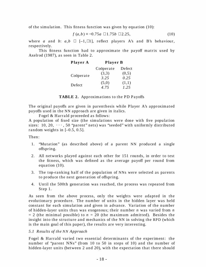
of the simulation. This fitness function was given by equation (10):
f (a,b) = −0.75a + 1.75b + 2.25, (10)
where a and b: a,b ∈ [–1,+1], reflect players A’s and B’s behaviour,respectively.
This fitness function had to approximate the payoff matrix used byAxelrod (1987), as seen in Table 2.
Player A Player BCooperate Defect
(3,3) (0,5)Cooperate 3.25 0.25(5,0) (1,1)Defect 4.75 1.25
TABLE 2. Approximations to the PD Payoffs
The original payoffs are given in parenthesis while Player A’s approximatedpayoffs used in the NN approach are given in italics.
Fogel & Harrald proceeded as follows:A population of fixed size (the simulations were done with five populationsizes: 10, 20, . . . , 50 “parent” nets) was “seeded” with uniformly distributedrandom weights in [–0.5, 0.5].
Then:
1. “Mutation” (as described above) of a parent NN produced a singleoffspring.
2. All networks played against each other for 151 rounds, in order to testthe fitness, which was defined as the average payoff per round fromequation (10).
3. The top-ranking half of the population of NNs were selected as parentsto produce the next generation of offspring.
4. Until the 500th generation was reached, the process was repeated fromStep 1.
As seen from the above process, only the weights were adapted in theevolutionary procedure. The number of units in the hidden layer was heldconstant for each simulation and given in advance. Variation of the numberof hidden-layer units thus was exogenous; their number n was varied from n= 2 (the minimal possible) to n = 20 (the maximum admitted). Besides theinsight into the structure and mechanics of the NN in solving the RPD (whichis the main goal of this paper), the results are very interesting.
5.1 Results of the NN Approach
Fogel & Harrald varied two essential determinants of the experiment: thenumber of “parent NNs” (from 10 to 50 in steps of 10) and the number ofhidden-layer units (between 2 and 20), with the expectation that there should
- 18 -

be enough units in the hidden layer to enable sufficient behaviouralcomplexity. Thus, it hardly could be expected that a 6–2–1 NN (a short-handway of describing a NN with 6 input units, 2 hidden units and 1 output unit)would develop stable cooperative behaviour, and in fact it did not. On theother hand, a 6–20–1 NN most of the time showed — in Fogel & Harrald’swords — “fairly” persistent cooperative behaviour, and thus, to a certainextent, met the expectations, but could never establish a stable regime ofcooperation like Axelrod’s paradigmatic results. Although delivering the bestperformance of all tested architectures, the level of cooperation as measuredby the average payoffs was below what could be expected if all had alwayscooperated, and was worse than the Axelrod simulations.
There also seemed to exist an increasing probability of stabilizingcooperation with population size, but it was never stable, and could insteadproduce a sudden breakdown of cooperation, even after generation 1,200,from which it mostly did not recover.
5.2 Critique and Conclusions to the NN Approach
The results described above are surprising, and invite further investigation.A standard critique of the NN approach could be of the simulation design,which makes the evolutionary adaptations of weights and the networkcomplexity (given here only by the number n of hidden units) disjunct parts ofthe trials. If we extrapolate “normal” NN experiences, then there is aninherent dependence of weights and NN structure with respect to an optimaladaptation. In this sense only coadaptation would make sense, but this wasnot implemented in the experiment of Fogel & Harrald’s.
The results contrast with the GA results, but give also rise tospeculation about the different approaches of both methods: GAs work by astrict zero–one mapping within the genome string, while the above NN designadmits of real values varying between –1 or +1, thus weakening theboundedness or “degree of determinism” within the model, and possiblyallowing a more “fuzzy” behavioural context between the opponents.
Unfortunately, the authors of this paper do not possess an appropriateNN simulator which would enable us to rerun the above experiments and toadd elements or alter the design with respect to the above speculation, whichcould be tested by the so-called gain γ (i.e. the “steepness” of the sigmoidtransfer function, cf equation (3)) of a unit and thus changing the behaviourgradually towards a more discrete (digital) one. Thus, these remarks canonly be tentative and remain speculative.
6. Comparison of the Two Approaches and Concluding Remarks
As the results may suggest, a close interpretation may be that the RPD ismore the domain of the GA approach than that of the NN. In Section 3.3 wemention that the NN architecture must be specified with respect to the data itprocesses. Indeed, it is one of the wisdoms of NN expertise that the datastructure will require — and, if allowed by pruning, will form — its specialarchitectural form. In the above NN example, there was only limitedopportunity for achieve this — only the number of hidden units.
- 19 -
Moreover, the NN tried to approximate the overt zero–one type of RPDproblem — each player has only two choices, either Cooperate (C ≡ 0) orDefect (D ≡ 1) — at two points by real-valued functions:
— in simulating the integer-valued payoffs by a “best” equation, whichprovides for a much more linear approach (Table 2), as does the original(Table 1) used by the GA approach;
— in approximating the zero–one actions by real-valued numbers.
So the NN formulation is not as close to the problem as is the GAstructure, which uses a zero–one approach and thus operates much moreclosely to the focus of the RPD problem. It may well be that the contrast ofzero–one encoding of the GA solution against the more fuzzy, real-valuedencoding of the NN are sufficient to explain the lower stability of performanceof the NN compared to the GA, since it is readily imagined that the basin ofattraction for the final solution of a typical zero–one problem such as the RPDis much more clear-cut and thus much more stable than it is for a smooth“landscape” explored by a NN. This conclusion may well be reversed for aproblem which is formulated in real-valued solutions, such as the forecast of astock price. It is certainly the case, at least when using the binary-stringrepresentation of solutions with the GA, that the number of significant digitsis in general a prior decision: the length of the bit string places an upperlimit on the precision of the solutions.
In conclusion we make some more general observations. Evolutionaryalgorithms are well suited for high-dimensional, complex search spaces. WithEAs there are no restrictive requirements on the objective function (if oneexists), such as continuity, smoothness, or differentiability; indeed, there maybe no explicit objective function at all. The basic EA forms are broadlyapplicable across many diverse domains, and, with flexible customising, it ispossible to incorporate more knowledge of the domain, although such domainknowledge is not required. They have been found to be reliable, and areeasily combined with other techniques, to form so-called hybrid techniques.They make efficient use of parallel-processing computer hardware.
Evolutionary algorithms are heuristic in nature (with no guarantee ofreaching the global optimum in a specific time); indeed, finding good settingsfor strategy parameters (population size and structure, crossover rate,mutation rate in the GA) can require some experience. They are oftenineffective in fine-tuning the final solution. The theory of EAs is still beingdeveloped. They have comparatively high CPU requirements, although withMoore’s law in operation, this is less and less a problem.
7. References
Adeli, H., & Hung S.-L. (1995) Machine Learning: Neural Networks, GeneticAlgorithms, and Fuzzy Systems, NY: Wiley.
Axelrod, R. (1984) The Evolution of Cooperation, New York: Basic Books.
Axelrod, R. (1987) The evolution of strategies in the iterated Prisoner’sDilemma, in: Genetic Algorithms and Simulated Annealing, L. Davis (ed.)
- 20 -

(Pitman, London) pp.32–41.
Bertsekas, D.P., Tsitsiklis, J.N. (1996), Neuro-Dynamic Programming,Belmont, Mass.: Athena Scientific.
Bethke, A.D. (1981) Genetic algorithms as function optimizers. (Doctoraldissertation, University of Michigan). Dissertation Abstracts International41(9): 3,503B. (University Microfilms No. 81–06,101)
Brady, R.M. (1985) Optimization strategies gleaned from biological evolution.Nature 317: 804–806.
Cho, I.-K. (1995) Perceptrons play the repeated Prisoner’s Dilemma, Journalof Economic Theory, 67: 266–284.
Davis, L. (1991) A genetic algorithms tutorial. In: Davis L. (ed.) Handbook ofGenetic Algorithms. New York: Van Nostrand Reinhold.
Dupre, J. (ed.) (1987) The Latest on the Best: Essays on Evolution andOptimality. Cambridge: MIT Press.
Fogel, D.B., Harrald, P.G. (1994) Evolving continuous behaviors in theiterated Prisoner’s Dilemma in: Sebald, A., Fogel, L. (eds.) The ThirdAnnual Conference on Evolutionary Programming, Singapore: WorldScientific, pp.119–130.
Fujiki, C., Dickinson, J. (1987) Using the genetic algorithm to generate Lispsource code to solve the Prisoner’s Dilemma. In: Grefenstette J.J. (ed.)Genetic Algorithms and their Applications, Proceedings of the 2nd.International Conference on Genetic Algorithms. Hillsdale, N.J.:Lawrence Erlbaum.
Goldberg, D.E. (1989) Genetic Algorithms in Search, Optimization andMachine Learning, Reading, Mass.: Addison-Wesley
Gould S.J. 1996, Full House: The Spread of Excellence from Plato to Darwin,New York: Harmony Books. (Also, for some reason, published in Londonas Life’s Grandeur.)
Grefenstette, J.J. (1987) A User’s Guide to GENESIS. Navy Center forApplication Research in Artificial Intelligence, Naval ResearchLaboratories, mimeo., Washington D.C.
Hebb, D. (1949) The Organization of Behavior, New York: Wiley.
Holland, J.H. (1975) Adaptation in Natural and Artificial Systems. AnnArbor: Univ. of Michigan Press. (A second edition was published in 1992:Cambridge: MIT Press.)
Holland, J.H. (1984) Genetic algorithms and adaptation. In: Selfridge O.,Rissland E., & Arbib M.A. (eds.) Adaptive Control of Ill-Defined Systems.New York: Plenum.
Koza, J.R. (1992) Genetic Programming, Cambridge: MIT Press.
- 21 -

Langton, C.G., Taylor, C., Farmer, J.D., Rasmussen, S. (ed.) (1992) ArtificialLife II, Reading: Addison-Wesley.
Marks, R.E. (1989) Niche strategies: the Prisoner’s Dilemma computertournaments revisited. AGSM Working Paper 89–009.<http://www.agsm.unsw.edu.au/∼bobm/papers/niche.pdf>
Marks, R.E. (1992a) Breeding optimal strategies: optimal behaviour foroligopolists, Journal of Evolutionary Economics, 2: 17–38.
Marks, R.E. (1992b) Repeated games and finite automata in: Creedy, J.,Borland, J., Eichberger, J. (eds.) Recent Developments in Game Theory.Aldershot: Edward Elgar.
McCulloch, W.S., Pitts, W. (1943) A logical calculus of the ideas immanent innervous activity, Bulletin of Mathematical Biophysics 5.
Michalewicz, Z. (1994) Genetic Algorithms+Data Structures = EvolutionaryPrograms, Berlin: Springer Verlag, 2nd ed.
Miller, J.H. (1996) The coevolution of automata in the repeated Prisoner’sDilemma. Journal of Economic Behavior and Organization, 29: 87–112.
Minsky, M., Papert, S. (1969) Perceptrons, Cambridge: MIT Press.
Mitchell, M. (1996) An Introduction to Genetic Algorithms, Cambridge: MITPress.
Nissen, V. (1995) An overview of evolutionary algorithms in managementapplications, in Evolutionary Algorithms in Management Applications, ed.by J. Biethahn & V. Nissen, Berlin: Springer-Verlag, pp.44–97.
Nissen, V., Biethahn, J. (1995) An introduction to evolutionary algorithms, inEvolutionary Algorithms in Management Applications, ed. by J. Biethahn& V. Nissen, Berlin: Springer-Verlag, pp.3–43.
Rechenberg, I. (1973) Evolutionsstrategie. Optimierung technischer Systemenach Prinzipien der biologischen Evolution, Stuttgart: Frommann-Holtzboog.
Rumelhart, D.E., McClelland, J.L. (1986) Parallel Distributed Processing:Explorations in the Microstructure of Cognition, Vol. 1: Foundation, 2.Aufl., Cambridge: MIT Press.
Sargent, T.J. (1993) Bounded Rationality in Macroeconomics, Oxford: O.U.P.
Schaffer, J.D., Grefenstette, J.J. (1988) A critical review of geneticalgorithms. Mimeo.
Schwefel, H.P., Manner, R., (1991) Parallel Problem Solving from Nature,(Lecture Notes in Computer Science 496). Berlin: Springer-Verlag.
Sebald, A., Fogel, L. (eds.) (1994) The Third Annual Conference onEvolutionary Programming, Singapore: World Scientific.
- 22 -
White, H. (1992) Artificial Neural Networks: Approximation and Learning,Oxford: Basil Blackwell.
Widrow, B., Hoff, M.E. (1960) Adaptive switching circuits, In: Institute ofRadio Engineers, Western Electronic Show and Convention, ConventionRecord, Part 4, pp.96–104.
- 23 -