Embed Size (px)
Citation preview
GENERATION OF TTT AND CCT CURVES
FOR CAST TI-6AL-4V ALLOY
By
YIN KUANG
A THESIS PRESENTED TO THE GRADUATE SCHOOL OF THE UNIVERSITY OF FLORIDA IN PARTIAL FULFILLMENT
OF THE REQUIREMENTS FOR THE DEGREE OF MASTER OF SCIENCE
UNIVERSITY OF FLORIDA
2004

Copyright 2004
by
Yin Kuang

This thesis is dedicated to my family with love and gratitude.
ACKNOWLEDGMENTS
First and foremost, I would like to express my sincere gratitude to my advisor, Dr.
Michael Kaufman, for his invaluable guidance, encouragement, and support through my
graduate work at the University of Florida. Working in his group is a great pleasure and
learning experience.
Special thanks go to Dr. James Cotton from Boeing Aerospace Corporation who
supported this project. I want to thank Dr. Robert DeHoff and Dr. Gerhard Fuchs, for
serving on my thesis committees and for their valuable classes. Many thanks are due to
my colleagues, Junyeon, Jerry, and Tibisay, and all other members in our group, for their
friendly help and support.
Finally, I would like to thank my husband and my parents. My husband, who is
always there supporting me and helping me, makes my pursuit of the master’s degree
such a happy and rewarding journey. Without him, I could never have come to this far
and have done this thesis. My parents, who now still live far away from me in my home
country, always can warm and encourage me and help me go through all the difficulties.
iv

TABLE OF CONTENTS page ACKNOWLEDGMENTS ................................................................................................. iv
LIST OF TABLES............................................................................................................ vii
LIST OF FIGURES ......................................................................................................... viii
ABSTRACT...................................................................................................................... xii
CHAPTER
1 INTRODUCTION ........................................................................................................1
1.1 Metallurgy Properties of Ti-6Al-4V.......................................................................1 1.2 Purpose of the study................................................................................................3
2 LITERATURE REVIEW .............................................................................................5
2.1 TTT Curves for Ti-6Al-4V.....................................................................................7 2.1.1 First Published TTT Diagram for Ti-6Al-4V...............................................7 2.1.2 TTT Curves from Microstructural Examinations.........................................8 2.1.3 TTT Curves from Microhardness Examinations..........................................9 2.1.4 Neural Network Approach .........................................................................12 2.1.5 Computer Modeling....................................................................................14 2.1.6 Resistivity Study Based on Computer Modeling .......................................14
2.2 CCT Curves for Ti-6Al-4V ..................................................................................16 2.3 Conduction of Heat in Semi-infinite Solid ...........................................................19
3 EXPERIMENTS.........................................................................................................21
3.1 Isothermal Heat Treatment Experiments ..............................................................21 3.2 Instrumented Jominy End Quench (JEQ) Experiments........................................22 3.3 Complementary Continuous Cooling Tests..........................................................26 3.4 Optical Microscopy ..............................................................................................26 3.5 Scanning Electron Microscopy.............................................................................27 3.6 Transmission Electron Microscopy ......................................................................27
v

4 RESULTS...................................................................................................................28
4.1 Test Results from the Isothermal Heat Treatment ................................................28 4.2 Test Results from Jominy End Quench ................................................................37
4.2.1 Temperature-Time Data .............................................................................37 4.2.2 Microstructures along the JEQ Sample ......................................................40 4.2.3 Rockwell C Hardness Data.........................................................................54
4.3 Continuous Cooling Data .....................................................................................56 5 ANALYSIS AND DISCUSSIONS ............................................................................64
5.1 Simulation of the Cooling Rates of Jominy End Quench Sample........................64 5.2 CCT Curves for Ti-6Al-4V ..................................................................................68 5.3 Analysis of the Shearing Direction in α Phase Formation....................................73 5.4 TTT Curve for Ti-6Al-4V ....................................................................................79
6 CONCLUSION...........................................................................................................80
LIST OF REFERENCES...................................................................................................81
BIOGRAPHICAL SKETCH .............................................................................................83
vi
LIST OF TABLES
Table page 1. Processing, Heat-treatment, Microstructure Summary for Ti-6Al-4V. .........................22
2. Physical Properties of Ti-6Al-4V and a Carbon Steel ..................................................65
3. Cooling Rates at some Interested Spots along JEQ Sample ..........................................66
vii
viii
LIST OF FIGURES
Figure page 2-1 Isothermal sections for the Ti-Al-V ternary system...................................................5
2-2 Time-Temperature Transformation Diagrams of certain Titanium Sheet-Rolling-Program Alloys .........................................................................................................8
2-3 TTT diagram for Ti-6Al-4V after holding at 1100ºC for 10 min and quenching into isothermal baths. Prior heat treatment is the solution treatment at 1100ºC for 30 min followed by quenching into iced brine. ......................................................................9
2-4 TTT diagrams for beta phase decomposition in Ti-6Al-4V specimens containing 10 at. Pct H . .............................................................................................................10
2-5 Dependence of the (a) nose temperature and (b) nose time for the beginning of the beta phase decomposition on the hydrogen concentration.......................................11
2-6 Calculated TTT diagrams for Ti-6Al-4V alloy with different oxygen levels .........13
2-7 Calculated time-temperature-transformation diagrams for Ti-6Al-4V. ...................16
2-8 Schematic continuous cooling diagram for Ti-6Al-4V β-solution treated at 1050ºC for 30 min [12] (Ms temperature due to Majdic and Ziegler ) ......................18
3-1 Samples before and after the isothermal treatments in the salt pots. .......................22
3-2 Home-made set up for Jominy End Quench test......................................................23
3-3 Schematic of the Jominy end quench sample instrumented with four thermocouples. .........................................................................................................24
3-4 Temperature-time data of the JEQ sample in tube furnace (left) were collected by a data acquisition system (right). ................................................................................24
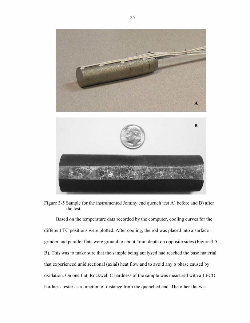
3-5 Sample for the instrumented Jominy end quench test A) before and B) after the test. ...........................................................................................................................25
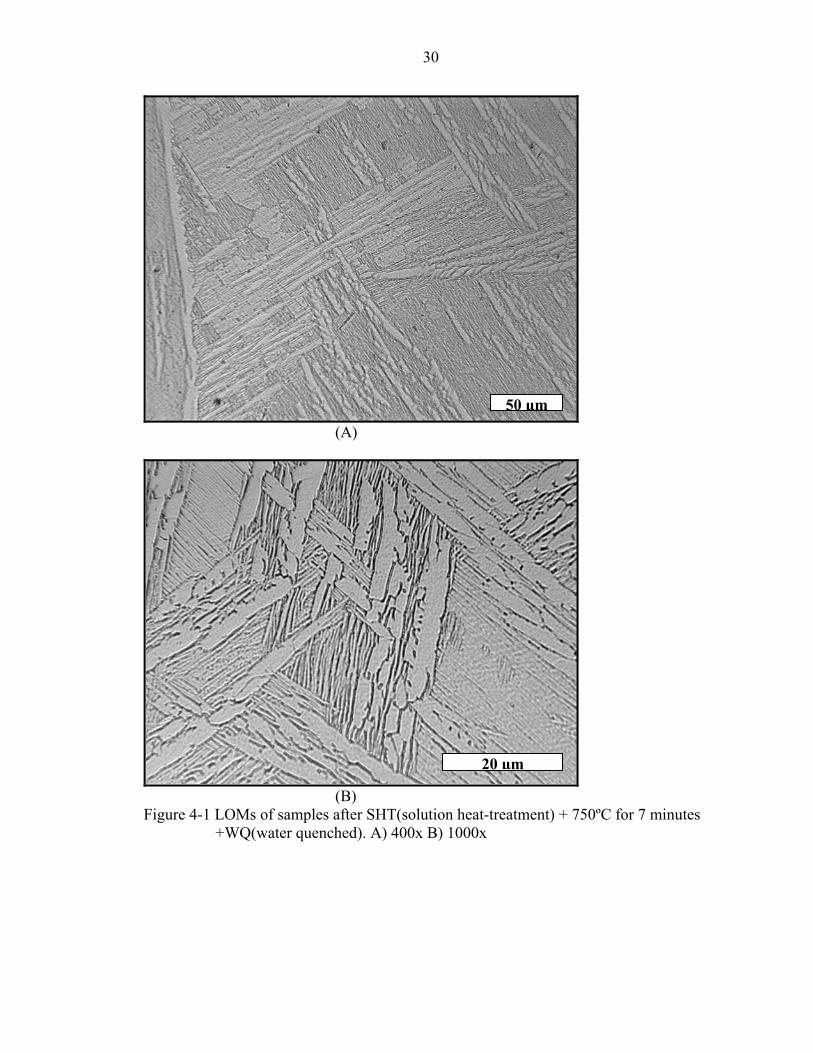
4-1 LOMs of samples after SHT(solution heat-treatment) + 750ºC for 7 minutes +WQ(water quenched). A) 400x B) 1000x..............................................................30
4-2 LOMs of samples after SHT + 750ºC for 17 minutes +WQ. A) 400x B) 1000x.....31
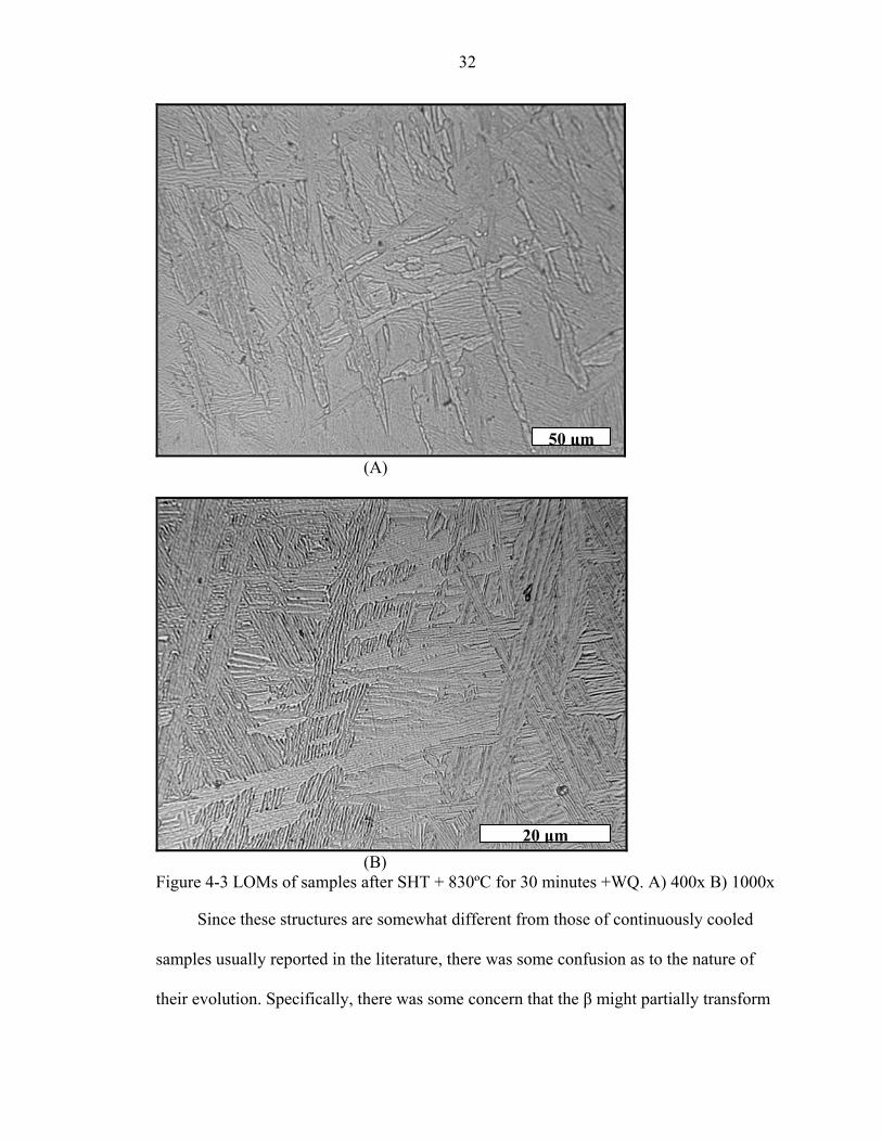
4-3 LOMs of samples after SHT + 830ºC for 30 minutes +WQ. A) 400x B) 1000x.....32
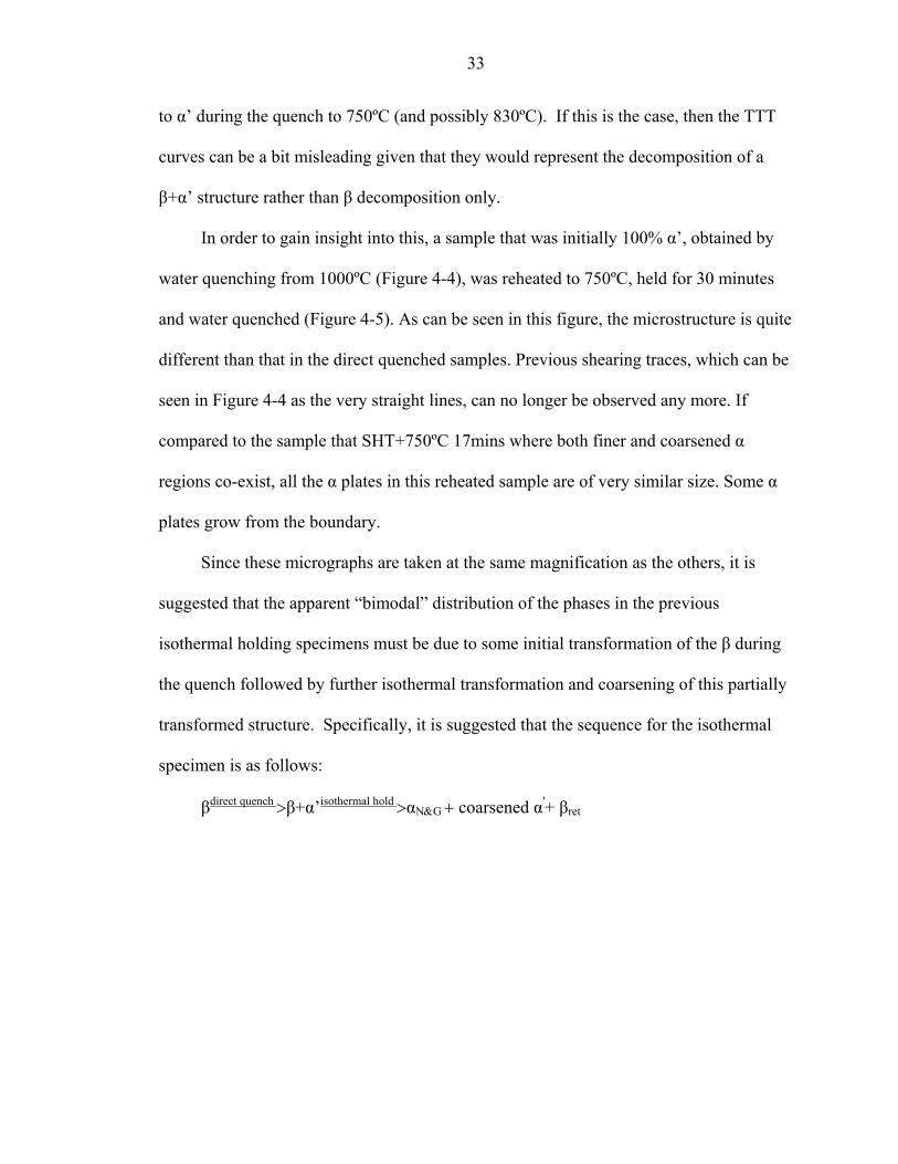
4-4 LOM of sample SHT + WQ. 1000x........................................................................34
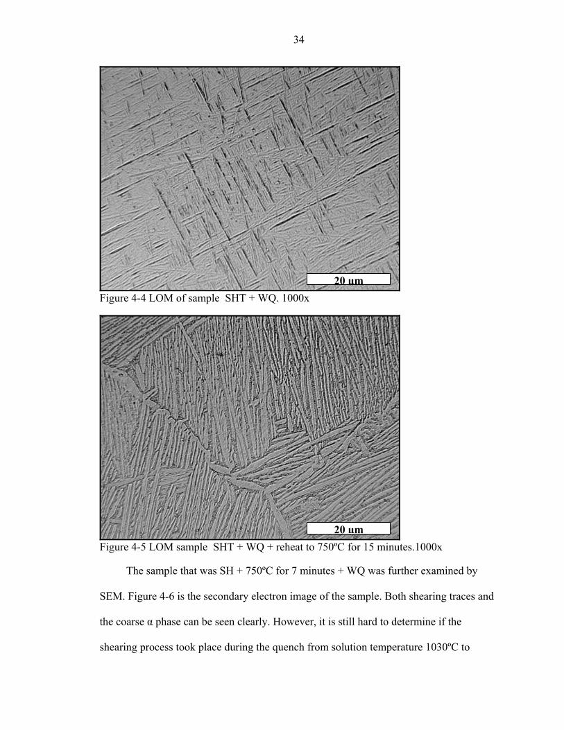
4-5 LOM sample SHT + WQ + reheat to 750ºC for 15 minutes.1000x........................34
4-6 SEM of sample SHT + 750ºC for 7 minutes + WQ .................................................35
4-7 SEM of sample SHT + 750ºC for 90 minutes + WQ ...............................................36
4-8 TEM of sample SHT + 750ºC for 17 minutes + WQ (A) Bright field image (B) SAD (selected area diffraction) pattern of the boundary of coarse α and finer α. .....................................................................................................................37
4-9 Experimental cooling curves from K-type thermocouples embedded in the JEQ sample.......................................................................................................................38
4-10 LabVIEW driver for data acquisition system A) reading data from thermocouples B) decimating data to four arrays .............................................................................39
4-11 LOM at 2mm from the quenched end, 400x, Rc= 40.5 ...........................................40
4-12 LOM at 9mm from the quenched end. Rc= 38.9 .....................................................41
4-13 LOM at 29mm from the quenched end. Rc= 37.4 ...................................................41
4-14 LOM at 27mm from the quenched end. ...................................................................42
4-15 LOM at 55mm from the quenched end. ...................................................................42
4-16 LOM at 66mm from the quenched end. Rc= 36.2 ...................................................43
4-17 LOM at 75mm from the quenched end. Rc= 36.8 ...................................................43
4-18 LOM at 90mm from the quenched end. Rc= 34.9 ...................................................44
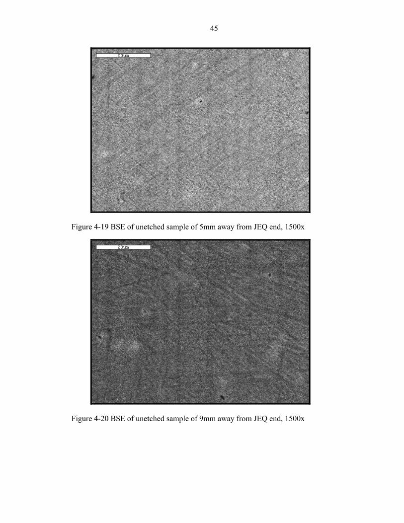
4-19 BSE of unetched sample of 5mm away from JEQ end, 1500x ................................45
4-20 BSE of unetched sample of 9mm away from JEQ end, 1500x ................................45
4-21 BSE of unetched sample of 12mm away from JEQ end, 1500x ..............................46
4-22 BSE of unetched sample of 16mm away from JEQ end, 1500x ..............................46
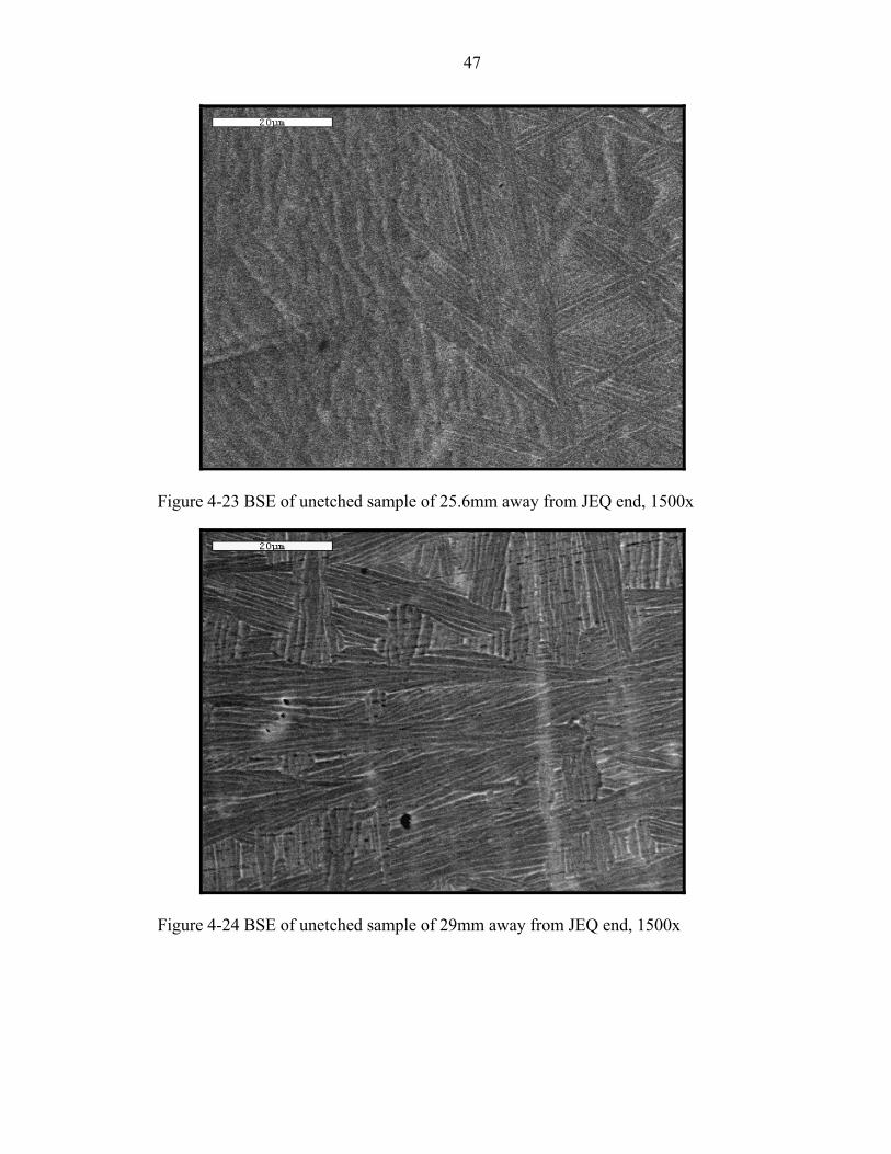
4-23 BSE of unetched sample of 25.6mm away from JEQ end, 1500x ...........................47
4-24 BSE of unetched sample of 29mm away from JEQ end, 1500x ..............................47
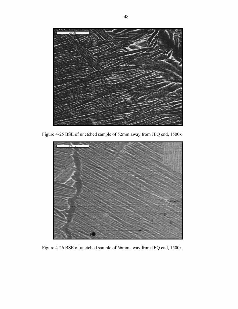
4-25 BSE of unetched sample of 52mm away from JEQ end, 1500x ..............................48
ix
4-26 BSE of unetched sample of 66mm away from JEQ end, 1500x ..............................48
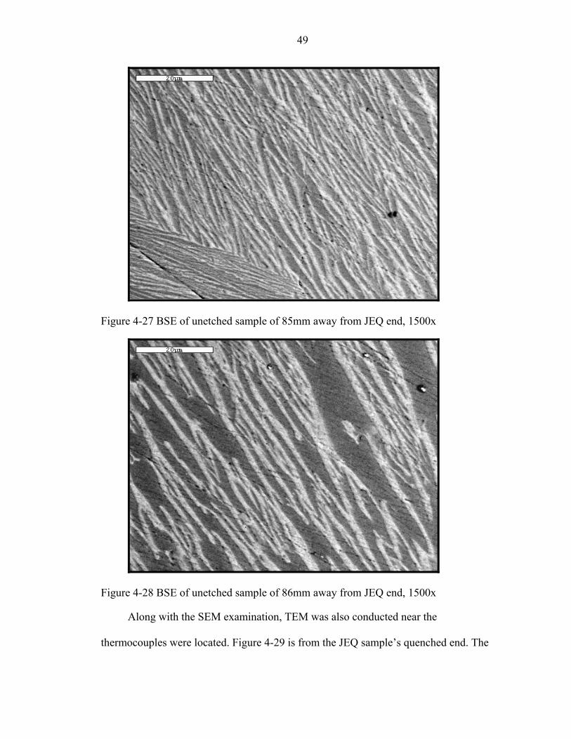
4-27 BSE of unetched sample of 85mm away from JEQ end, 1500x ..............................49
4-28 BSE of unetched sample of 86mm away from JEQ end, 1500x ..............................49
4-29 TEM of the quenched end, martensite structure A) 5,000X; B) 20,000X ...............51
4-30 TEM of location 2 (27mm away from quenched end). ............................................52
4-31 TEM of location 3 (55mm away from quenched end) α grains grows at different directions 5,000X .....................................................................................................53
4-32 TEM of location 3 (55mm away from quenched end) α grains grows at different directions with β phase in between the α-α grain boundary 20,000X......................53
4-33 TEM of location 4 (87mm away from quenched end) more coarsened α grains 3,000X ......................................................................................................................54
4-34 Hardness vs. position for the Ti-6Al-4V JEQ specimens from two same A) and B) conditions test...........................................................................................................55
4-35 LOM of samples after 30 minutes solution treatment at 1030C, air cooled to 900ºC and water quenched. .................................................................................................56
4-36 LOM of samples after 30 minutes solution treatment at 1030C, air cooled to 800ºC and water quenched. .................................................................................................57
4-37 LOM of samples after 30 minutes solution treatment at 1030C, air cooled to 700ºC and water quenched. .................................................................................................57
4-38 BSE of unetched sample after 30 minutes solution treatment at 1030C, air cooled to 900ºC and water quenched. ..................................................................................58
4-39 BSE of unetched samples after 30 minutes solution treatment at 1030ºC, air cooled to 800ºC and water quenched. ..................................................................................59
4-40 BSE of unetched samples after 30 minutes solution treatment at 1030ºC, air cooled to 700ºC and water quenched.. .................................................................................59
4-41 LOM of sample after 30 minutes solution treatment at 1030ºC, furnace cooling to 900ºC, and water quenching.....................................................................................60
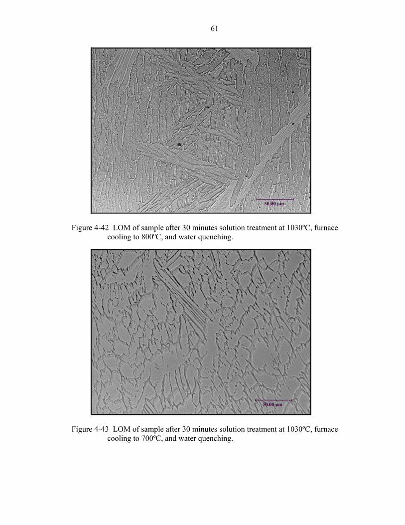
4-42 LOM of sample after 30 minutes solution treatment at 1030ºC, furnace cooling to 800ºC, and water quenching.....................................................................................61
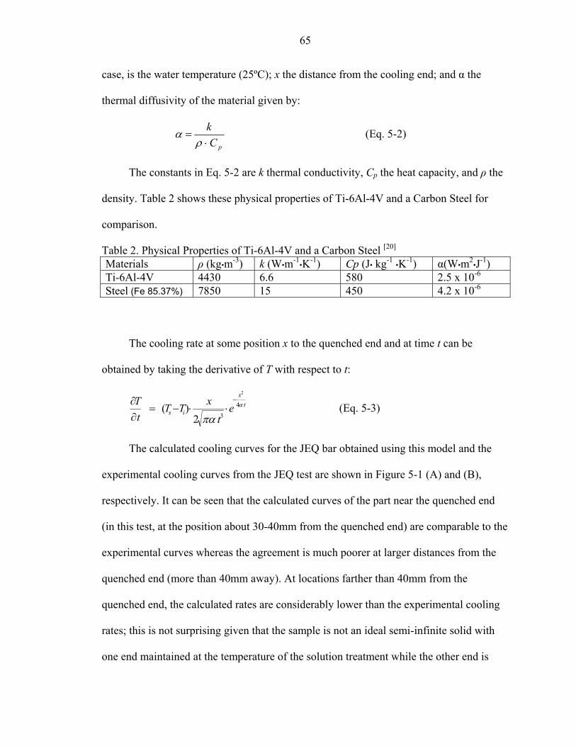
4-43 LOM of sample after 30 minutes solution treatment at 1030ºC, furnace cooling to 700ºC, and water quenching.....................................................................................61
x
4-44 BSE of sample after 30 minutes solution treatment at 1030ºC, furnace cooling to 900ºC and water quenching......................................................................................62
4-45 BSE of samples after 30 minutes solution treatment at 1030ºC, furnace cooling to 800ºC and water quenching......................................................................................63
4-46 BSE of samples after 30 minutes solution treatment at 1030ºC, furnace cooling to 700ºC and water quenching......................................................................................63
5-1 Cooling curves of JEQ sample A) calculated cooling curves using the semi-infinite solid heat transfer model; B) experimental cooling curves acquired from temperature data acquisition system during the JEQ test.........................................67
5-2 Experimental CCT curves for alloy Ti-6Al-4V.. .....................................................69
5-3 LOM of quenched end sample. ................................................................................71
5-4 BSE image of sample 24mm from quenched end. ...................................................71
5-5 TEM micrograph and the corresponding electron diffraction patterns for the quenched end at B=<111> of prior β.. .....................................................................74
5-6 TEM micrograph and the corresponding electron diffraction patterns for the quenched end of the same area of 5-5 at B=<011> of the prior β phase..................75
5-7 TEM of the sample at 27mm from the quenched end with at B=<11-20> of α phase. The directions of the α plates were analyzed. ..............................................76
5-8 TEM of the sample at 27mm from the quenched end of the same area of Figure 5-7 at B=<10-10> of α phase. The directions of the α plates were analyzed. ................77
5-9 Stereographic analysis shows the relationship between the A) directions of martensite needle-like laths lies in the circled region, and B) directions of traces of the α laths lies in the regions that circled. ................................................................78
xi
Abstract of Thesis Presented to the Graduate School
of the University of Florida in Partial Fulfillment of the Requirements for the Degree of Master of Science
GENERATION OF TTT AND CCT CURVES FOR CAST TI-6AL-4V ALLOY
By
Yin Kuang
August 2004
Chair: Michael Kaufman Major Department: Materials Science and Engineering
Although Ti-6Al-4V is the most commonly used titanium alloy and plenty of
efforts have been made to generate the TTT and CCT curves for it, there is no published
TTT or CCT curves that have been widely accepted. In this project, we aimed to generate
the TTT and CCT curves for Ti-6Al-4V alloy based on the microstructures analysis of the
isothermal treatments, Jominy end quench, and continuous cooling experiments.
A CCT curve for Ti-6Al-4V alloy is generated. A temperature-time acquisition
system was constructed and operated by a LabVIEW driver. The experimental and
theoretical cooling curves for this alloy were compared and the cooling rates of some
specific positions on the JEQ bar were predicted. The sample that has a larger cooling
rate than that at 5mm of JEQ bar (~150ºC/sec) will form a non-diffusional α phase, a
shearing only phase, i.e., the martensite α’. The sample that has a lower cooling rate than
3ºC/sec will form 100 pct nucleation and growth α phase. The α phase formed in this area
has a basket-weave structure. When the sample has a cooling rate between 150ºC/sec and
xii

3ºC/sec, it will form α plates by shearing followed by diffusion growth or a mixed
shearing and diffusion process. This α phase has no basket-weave structure and the grains
have relatively straight sides. Rockwell C hardness does not change much except that the
hardness of α’ is relatively high.
Since the Ms is proved to be between 800ºC and 900ºC, TTT curves for Ti-6Al-4V
alloy should be drawn between Ms (800-900ºC) and β transus (995ºC). The incubation
time for β phase decomposition to α phase is extremely short.
This work is supported by Boeing Aerospace Corporation. Currently, Ti-6Al-4V is
of great interest in the development of the F/A-22 Raptor.
xiii
CHAPTER 1 INTRODUCTION
For decades, titanium and titanium alloys have been desirable and essential
materials. The combination of high strength, stiffness, good toughness, low density, and
good corrosion resistance provided by various titanium alloys at low to elevated
temperatures allows weight savings in aerospace structures and other high-performance
applications. Ti-6Al-4V is the most commonly used titanium alloy for structural
applications in high-performance military aircraft. Ti-6Al-4V is unique in that it
combines attractive properties with inherent workability (which allows it to be produced
in all types of mill products, in both large and small sizes), good shop fabricability
(which allows the mill products to be made into complex hardware), and the production
experience and commercial availability that lead to reliable and economic usage. Thus,
Ti-6Al-4V has become the standard alloy against which other alloys must be compared
when selecting a titanium alloy (or custom designing one) for a specific application. Ti-
6Al-4V is also the standard alloy selected for castings that must exhibit superior
strength[1].
1.1 Metallurgy Properties of Ti-6Al-4V
At the β transus temperature where the transformation to β on heating is complete,
titanium alloys undergo an allotropic transformation upon cooling, changing from a
close-packed hexagonal (hcp) crystal structure (α phase) to a body-centered cubic (bcc)
crystal structure (β phase). Based on the predominant phases present in the
microstructure, titanium alloys are classified into three major categories: alpha, alpha-
1
2
beta, and beta alloys. Ti-6Al-4V belongs to the alpha-beta family where both the
hexagonal alpha phase and the bcc beta phase co-exist at room temperature. Therefore,
the considerable microstructural variation of Ti-6Al-4V can be achieved since the alpha,
retained beta, and transformed beta constituents can exist in different forms, ranging from
equiaxed to acicular or some combination of both.
Acicular α is the most common transformation product formed from β during
cooling and is produced by nucleation and growth along one or several sets of preferred
crystallographic planes in the prior beta matrix. Sometimes, the acicular α has a basket-
weave appearance, which is characteristic of a Widmanstätten structure. Alpha prime (α’)
martensite is a non-equilibrium supersaturated alpha structure produced by diffusionless
(martensitic) transformation of beta. The needle-like structure is similar in appearance
and in mode of formation to martensite in steel. In Ti-6Al-4V, the differences between
alpha prime and acicular alpha are two-fold:
• The α and α’ compositions are different; i.e., the α’ has the same composition as the prior β, resulting from diffusionless process; while the acicular alpha is the production of diffusion.
• The α’ laths/plates tend to have very straight sides while the acicular α has curved sides.
Some equilibrium beta is present at room temperature in alpha-beta alloys. The
equilibrium beta usually is present between the grains of equilibrium alpha. Non-
equilibrium beta, also called retained beta phase, can be produced in alpha-beta alloys
that contain enough beta-stabilizing elements to retain the beta phase at room temperature
on rapid cooling from between the alpha transus and beta transus temperatures. In this
case, the alloy composition must be such that the temperature for the start of martensite
formation is depressed to below room temperature.
3
While interstitial oxygen (an α stabilizers) raises the transformation temperature,
the hydrogen (β stabilizer) lowers it. On the other hand, metallic impurities or alloying
elements may also either raise or lower the transformation temperature. Since Ti-6Al-4V
is an α-β alloy that consists of α phase and retained or transformed β phase, it has a wide
range of microstructures. It is known that vanadium is isomorphous with β titanium and
that it has low solubility in α titanium and decreases the transformation temperature, so
vanadium is added to the Ti-6Al-4V alloy to stabilize the β phase and prevent or
minimize formation of intermetallic compounds, which could occur during
thermomechanical processing, heat treatment, or service at elevated temperature.
Aluminum is added to alloys because it improves the creep strength of the α phase. Also,
aluminum increases the transformation temperature and has significant solubility in both
the α and β phases [2]. In Ti-6Al-4V, vanadium is enriched in the β phase while aluminum
is distributed approximately equally between the α and β phases.
The β to α phase transformation in Ti-6Al-4V is typically initiated at 995°C
(1825°F) [2]. The orientation of the α plates is related to the parent just below the β
transus β phase through one of the 12 possible variants of the Burgers orientation
relationship [3, 4]
{110}β// (0001)α
<111>β// <11-20>α
1.2 Purpose of the study
This work is supported by Boeing Aerospace Corporation. Currently, cast Ti-6Al-
4V is of great interest to them in the development of the F/A-22 Raptor. The
microstructure of the cast Ti-6Al-4V depends heavily on the cooling rate of the liquid and
4
the subsequent solid-state cooling and the heat treatments that follow. Practically, there is
a large variety of its microstructures produced by adjusting the cooling rate after solution
treatment above the β transus. Since mechanical properties are very sensitive to its
microstructures, time-temperature-transformation (TTT) and continuous cooling
transformation (CCT) diagrams are of great value to industry for achieving certain
mechanical demands. Although several efforts have been made to plot these curves for
Ti-6Al-4V, to our knowledge, there is no published TTT or CCT curves that are widely
accepted and practically used.
The purpose of this study was to determine such curves for the cast Ti-6Al-4V
material that is currently being developed for the F22 fighter. Initial isothermal
treatments were aimed at determining the TTT curves for this material. Modified Jominy
end quench (JEQ) experiments were then performed in an effort to determine the CCT
curves for this material [5]. Along with these tests, some complementary heat treatments
were conducted to verify the critical points in the phase transformation curves and to
fully understand the mechanism of the transformations. Finally, CCT curves for the cast
Ti-6Al-4V were generated according to the microstructural analysis of the tested sample;
also, concluding remarks on generating TTT curves are presented.
CHAPTER 2 LITERATURE REVIEW
Since TTT and CCT diagrams are useful for controlling the microstructures of
alloy Ti-6Al-4V, significant efforts have been made to generate such diagrams. Different
approaches, for example, resistivity measurements, surface relief, metallographic
analysis, and some computational methods like neural network computational model,
have been explored in the literature. In the following, we introduce these approaches
according to their experimental methods to generate TTT or CCT curves. Further, a
theory about conduction of heat in semi-infinite solid on which our further Jominy end
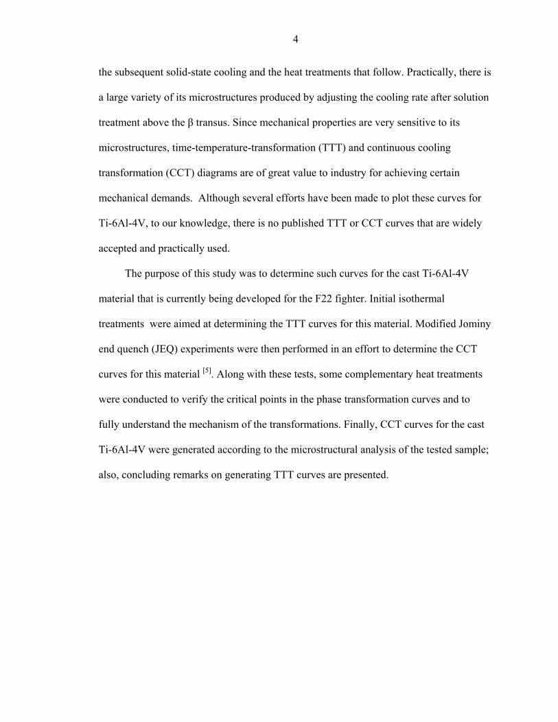
quench test is based will also be described. Before we start, it is important to note that the
following four phase diagrams are the basis that most of these approaches rely on.
•
Figure 2-1 A) 900ºC isothermal section for the Ti-Al-V ternary system.
5
6
B
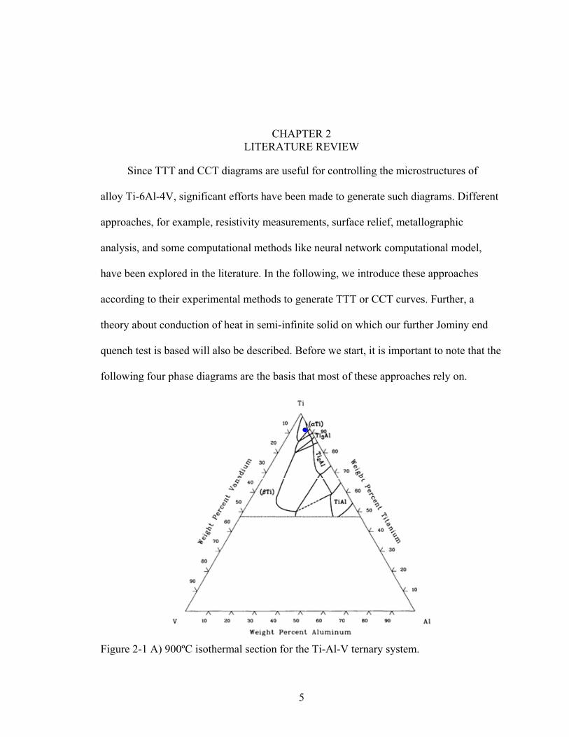
Figure 2-1 B) 980ºC and C) 1200ºC isother
•
C
•mal section for the Ti-Al-V ternary system.
7
D
•
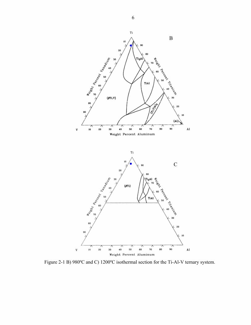
Figure 2-1 D) 1400ºC isothermal section for the Ti-Al-V ternary system.
2.1 TTT Curves for Ti-6Al-4V
In this section, the TTT curves published to date and the approaches taken to
generate them are described. These include both the experimental methods along with the
computational approach using neural networks.
2.1.1 First Published TTT Diagram for Ti-6Al-4V
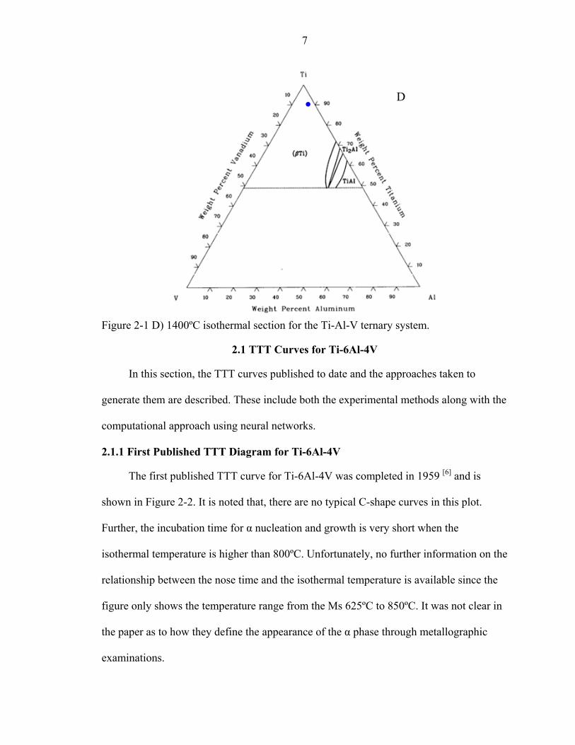
The first published TTT curve for Ti-6Al-4V was completed in 1959 [6] and is
shown in Figure 2-2. It is noted that, there are no typical C-shape curves in this plot.
Further, the incubation time for α nucleation and growth is very short when the
isothermal temperature is higher than 800ºC. Unfortunately, no further information on the
relationship between the nose time and the isothermal temperature is available since the
figure only shows the temperature range from the Ms 625ºC to 850ºC. It was not clear in
the paper as to how they define the appearance of the α phase through metallographic
examinations.

8
Figure 2-2 Time-Temperature Transformation Diagrams of certain Titanium Sheet-
Rolling-Program Alloys [6]
2.1.2 TTT Curves from Microstructural Examinations
In 1994, Ohmori et al. [7] used microstructural and surface relief observations to
investigate isothermal transformation characteristics of Ti-6Al-4V in order to obtain TTT
curves for the nucleation of primary α particles. Their experimental procedure was as
follows. Specimens were first heat treated in a dynamic argon atmosphere or in evacuated
quartz capsules at 1100ºC. They then were quenched into a lead or salt bath that was held
isothermally at temperatures between 700ºC and 925ºC. After that, they were further
quenched to room temperature. Microstructures of the specimens were revealed by slight
polishing and etching.
As seen from the TTT diagram in Figure 2-3, the nucleation of α exhibits a typical
C-curve in the temperature range between 700ºC and 950ºC. At 940ºC, primary α

9
particles nucleated heterogeneously at a β grain boundaries initially. When holding at
940ºC for longer time, e.g., 10h, α-plates grew from these grain boundary into the matrix
as side plates. Another condition they presented was for an alloy held at 925ºC for 15
minutes. The relatively large α-laths (~5µm) were counted as to plot the TTT diagram.
The authors didn’t present any microstructure of the sample being held at temperature
850ºC and lower. Thus, it is unclear how the lower temperature portion of the TTT curves
were defined.
Figure 2-3 TTT diagram for Ti-6Al-4V after holding at 1100ºC for 10 min and quenching into isothermal baths. Prior heat treatment is the solution treatment at 1100ºC for 30 min followed by quenching into iced brine [7].
2.1.3 TTT Curves from Microhardness Examinations
Because hydrogen, as an alloying element, changes the phase compositions and
kinetics of the phase transformations in titanium alloys, Qazi et al. [8] studied the
microstructure of Ti-6Al-4V-xH alloys and generated TTT curves for specimens
10
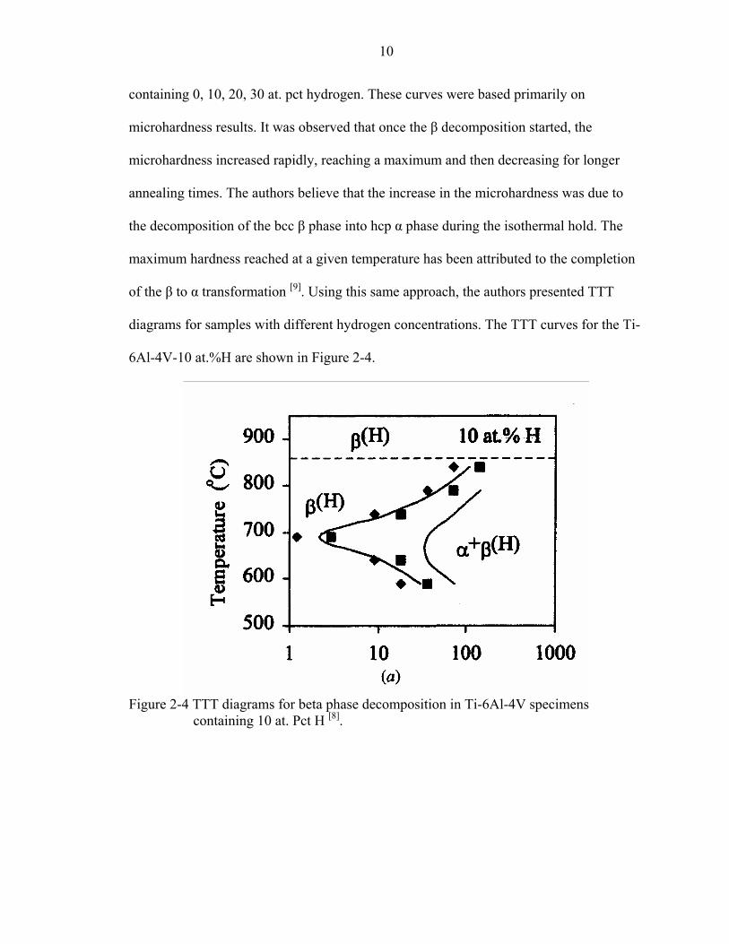
containing 0, 10, 20, 30 at. pct hydrogen. These curves were based primarily on
microhardness results. It was observed that once the β decomposition started, the
microhardness increased rapidly, reaching a maximum and then decreasing for longer
annealing times. The authors believe that the increase in the microhardness was due to
the decomposition of the bcc β phase into hcp α phase during the isothermal hold. The
maximum hardness reached at a given temperature has been attributed to the completion
of the β to α transformation [9]. Using this same approach, the authors presented TTT
diagrams for samples with different hydrogen concentrations. The TTT curves for the Ti-
6Al-4V-10 at.%H are shown in Figure 2-4.
Figure 2-4 TTT diagrams for beta phase decomposition in Ti-6Al-4V specimens
containing 10 at. Pct H [8].
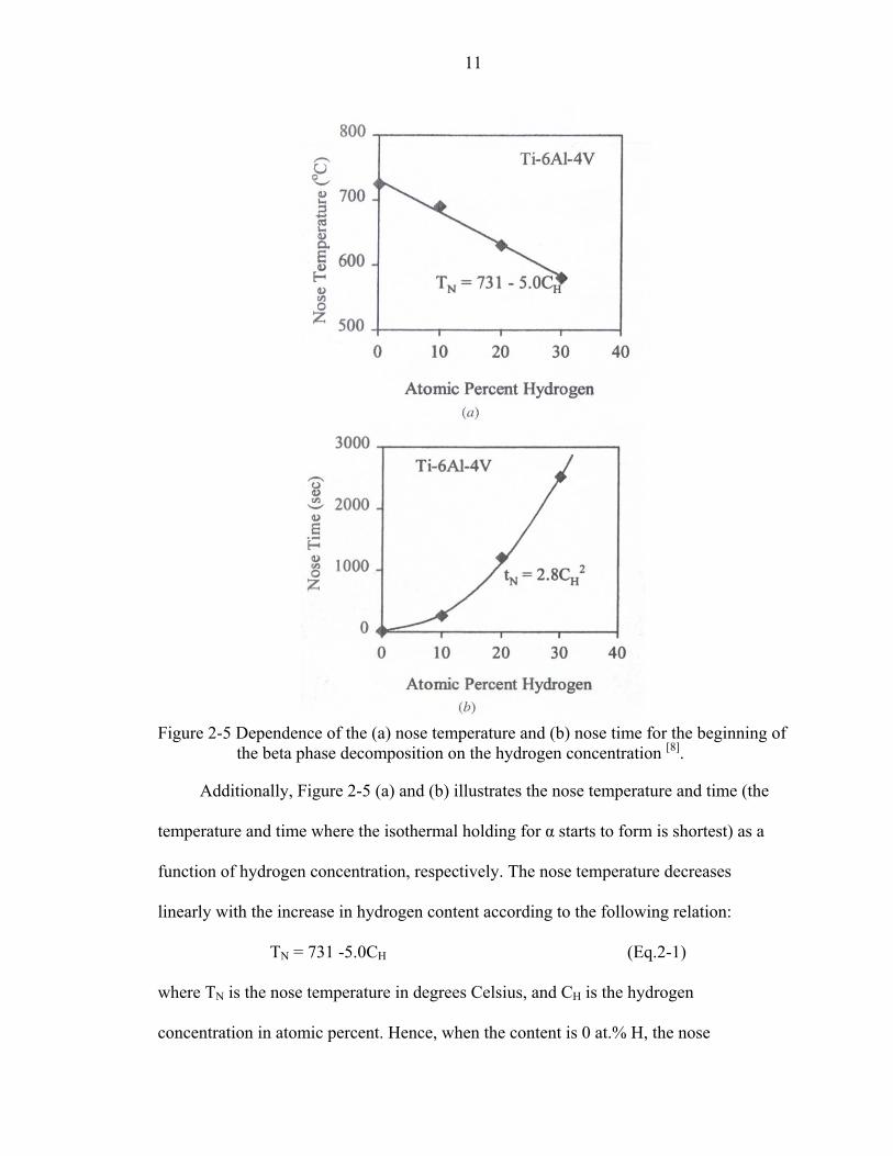
11
Figure 2-5 Dependence of the (a) nose temperature and (b) nose time for the beginning of
the beta phase decomposition on the hydrogen concentration [8].
Additionally, Figure 2-5 (a) and (b) illustrates the nose temperature and time (the
temperature and time where the isothermal holding for α starts to form is shortest) as a
function of hydrogen concentration, respectively. The nose temperature decreases
linearly with the increase in hydrogen content according to the following relation:
TN = 731 -5.0CH (Eq.2-1)
where TN is the nose temperature in degrees Celsius, and CH is the hydrogen
concentration in atomic percent. Hence, when the content is 0 at.% H, the nose
12
temperature is 731ºC. The nose time becomes longer when the hydrogen content
increases. This can be described by a quadratic relation:
tN = 2.8 CH2 (Eq.2-2)
where tN is the nose time in seconds. It is worth noting that when the content is 0 at.% H,
the nose time is 0 second and therefore can be ignored. This result is quite surprising.
2.1.4 Neural Network Approach
Recently, Malinov et al. proposed a computer modeling approach using an artificial
neural network to simulate the TTT diagram for Ti-6Al-4V [10]. They suggested that an
artificial neural network model can predict TTT diagrams for titanium alloys as a
function of their composition. This is basically achieved in three steps: first is data-base
collection with analysis and pre-processing of the data; second is training of the neural
network (includes choice of architecture, training functions, training algorithms and
parameters of the network) together with the test of the trained network; third is using the
trained neural network for simulation and prediction.
Their data-base was constructed by collecting available TTT diagrams for titanium
alloys. In total 189 TTT diagrams for different Ti alloys were collected from the
literature. Because neural networks typically work with numerical data, all 189 TTT
diagrams were scanned, put in electronic format and rescaled in one same scale. After
that, they were digitized by a set of numbers giving the relative increase of time when the
temperature was increased (above the nose temperature) or decrease (below the nose
temperature) by a certain ∆T. The Ms temperature was also included as another output to
complete the TTT diagrams.
Training of the neural network was performed using “Neural Network Toolbox” for
MATLAB. Three separate networks for training the temperature and the time of the
13
‘nose’ point, the description of the curves, and Ms temperature were created. These
networks are standard back-propagation multilayer feed-forward network created in
MATLAB. Two thirds of the data were used for training and one third for the finally test
of the neural network.
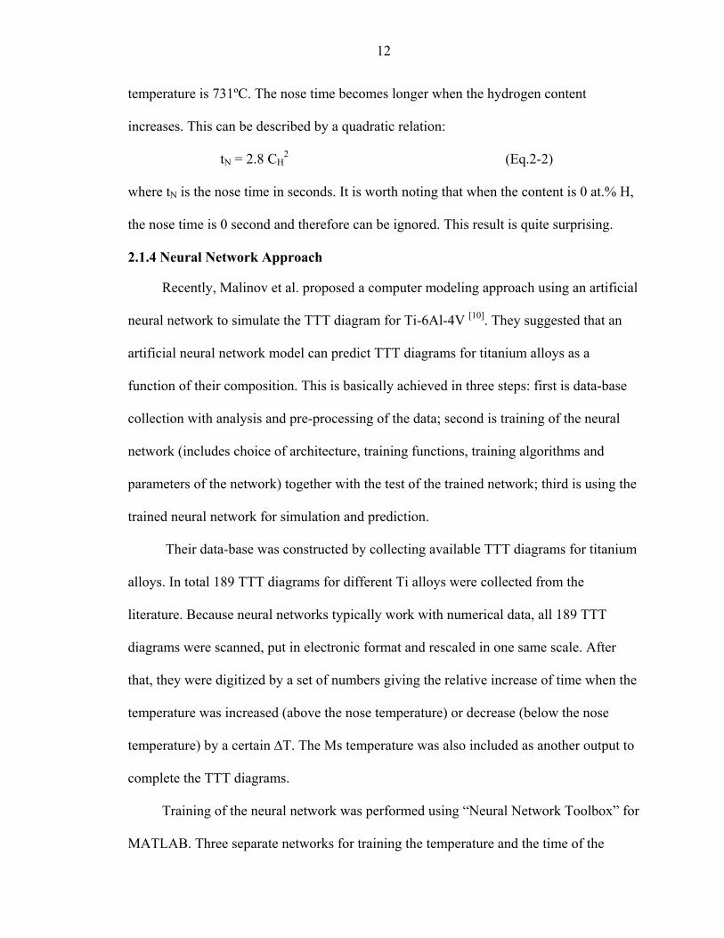
Ref [6]
Figure 2-6. Calculated TTT diagrams for Ti-6Al-4V alloy with different oxygen levels[10]
After training, the neural network can be used for simulation and prediction. TTT
curves of titanium alloys as a function of their composition were predicted. The
calculated TTT curves for Ti-6Al-4V with different oxygen levels from this model are
shown in Figure 2-6.
It is emphasized that this is the result of a purely statistical model not based on any
physical theory. On the one hand, this neural network itself is based on TTT results of
previous research, hence, the accuracy of the former test data play an essential role in the
14
predicted curves. However, even the authors accepted that, in some cases, there is a
contradiction between the TTT diagrams for the same alloy taken from different sources
and authors. On the other hand, although the authors used a totally of 189 TTT diagrams
for titanium alloys for training and testing their neural network, the actual number of TTT
diagrams for Ti-6Al-4V is very limited. It is not reasonable to use other titanium alloys
with a different composition to train the model of this particular alloy. Therefore, the
TTT diagram for the Ti-6Al-4V generated using neural networks is unreliable.
2.1.5 Computer Modeling
Since the experimental investigation and design of TTT curves are time consuming,
there is great interest in calculating these diagrams. The initial work on calculating the
TTT curves for Ti-6Al-4V was based on the Johnson-Mehl-Avrami expression [2] that
describes the diffusional transformations such as the transformation of austenite to either
ferrite, pearlite, or bainite in steel:
(Eq. 2-3) )exp(1 ntbv ⋅−−=
where v is the transformed volume fraction, t the time, b the reaction rate constant, and n
the Avrami index that describes the nucleation and growth mechanism. Both b and n are
temperature-dependent constants. The experimental C-shaped curves in the TTT
diagrams are approximated by spline functions when stored in the computer. The cooling
curve is approximated by a staircase, the step length being equal to the time step. The
phase transformation is then calculated isothermally during each time step.
2.1.6 Resistivity Study Based on Computer Modeling
Based on the Johnson-Mehl-Avrami theory, Malinov et al. proposed another
technique to derive the TTT diagrams [11]. A resistivity study of the kinetics of β -> α+β
15
transformation for Ti-6Al-4V alloy at isothermal conditions was embedded in the
framework of the JMA theory.
All samples were directly resistance heated with industry frequency electric current
employed. During the heating/cooling procedure, the relative changes of the electrical
resistivity were monitored and united with the temperature data. The changes of the
resistivity were suggested to be associated with the growth of the α, and possible with the
change of the composition of the α and β phases (e.g. the enrichment of the β phase with
vanadium). With this data, the curves of the resistivity versus isothermal holding time can
be converted to the curves of the amount of α versus time, given the known linear relation
between the relative changes of the electrical resistivity and the amount of the α phase.
The reaction rate constant b and the Avrami index n at different temperatures were
derived by logarithmic plots using Eq. 2-2. Practically, the experimental data were used
to build these logarithmic plots, which is ln(ln(1/(1-y))) versus ln(t). The slope of the
resulting straight line is the Avrami exponent n, while the intercept gives the value of b.
)exp(1)(
maxn
a
a btyv
tv−−== (Eq. 2-4)
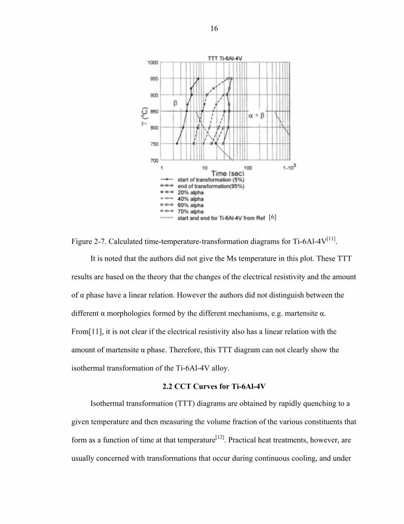
The TTT diagrams for Ti-6Al-4V alloy were then calculated and plotted in
Figure2-7.
It can be observed that there is no ‘nose’ point for the start of the β->α
transformation of Ti-6Al-4V from temperature of 950ºC to 750ºC. Two possible reasons
for this observation were suggested: 1) The high vanadium content of the alloy studied
causes a decrease in the β transition temperature. 2) Preprocessing and even early stages
of the transformation may take place on cooling from the β region to the temperature of
the isothermal exposure.
16
[6]
Figure 2-7. Calculated time-temperature-transformation diagrams for Ti-6Al-4V[11].
It is noted that the authors did not give the Ms temperature in this plot. These TTT
results are based on the theory that the changes of the electrical resistivity and the amount
of α phase have a linear relation. However the authors did not distinguish between the
different α morphologies formed by the different mechanisms, e.g. martensite α.
From[11], it is not clear if the electrical resistivity also has a linear relation with the
amount of martensite α phase. Therefore, this TTT diagram can not clearly show the
isothermal transformation of the Ti-6Al-4V alloy.
2.2 CCT Curves for Ti-6Al-4V
Isothermal transformation (TTT) diagrams are obtained by rapidly quenching to a
given temperature and then measuring the volume fraction of the various constituents that
form as a function of time at that temperature[12]. Practical heat treatments, however, are
usually concerned with transformations that occur during continuous cooling, and under

17
these conditions TTT diagrams, cannot be used to give the times and temperatures of the
various transformations. For this reason, a CCT diagram must be used. However, very
few CCT diagrams for Ti-6Al-4V are available.
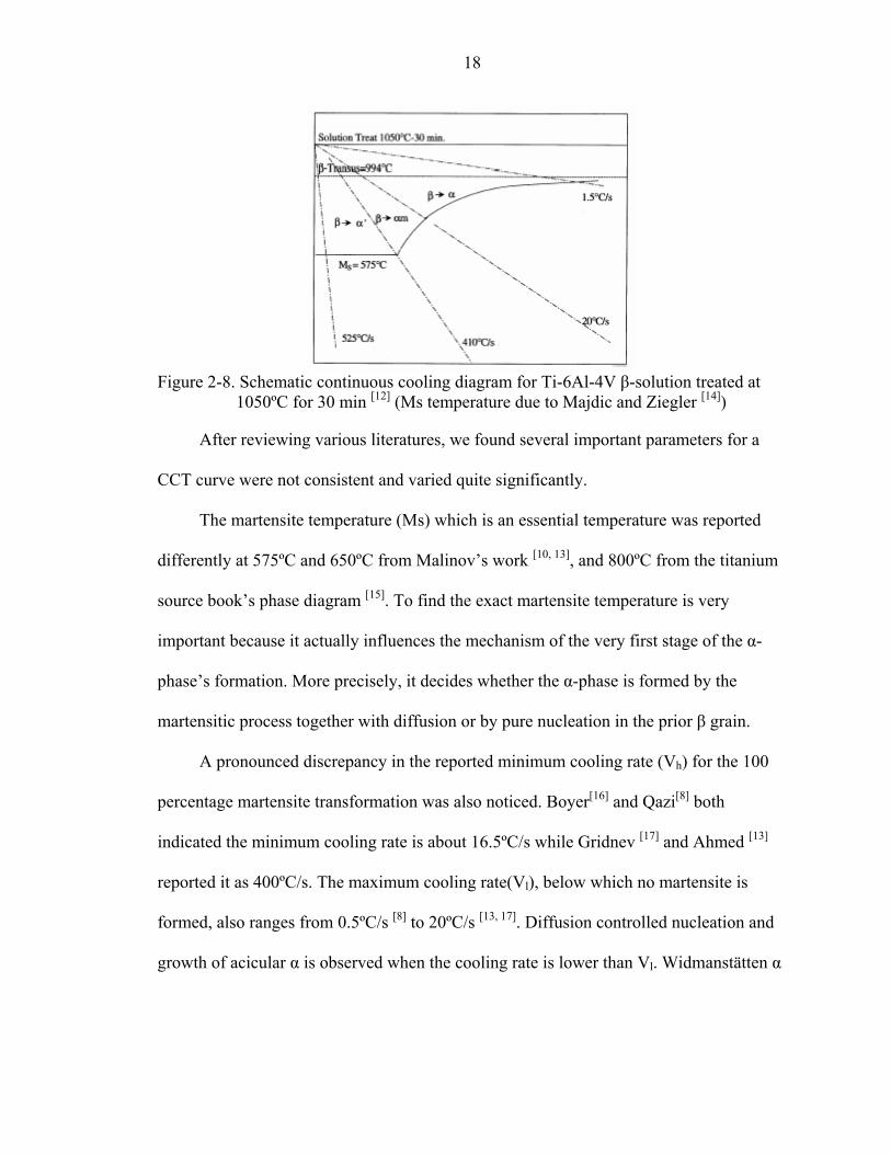
Ahmed et al.[13] used a refined Jominy end quench test to construct the CCT curves
for Ti-6Al-4V. A schematic continuous cooling diagram is shown in Figure 2-8.
According to their results, cooling rates above 410ºC/s result in a fully martensitic α’
microstructure; a massive transformation is observed between 410ºC/s and 20ºC/s; and
when the cooling rate is lower than 20ºC/s, the massive transformation is gradually
replaced by diffusion controlled Widmanstätten α formation. Optical microscopy was
used to characterize the microstructure.
The author suggested that at the cooling rate of 410ºC/s, a second α morphology
formed as a type 4 competitive massive transformation. This massive transformation
occurs at a sufficiently low transformation temperature where the trans-interphase
boundary diffusion rates associated with the massive transformation are high in
comparison with the volumetic diffusion rates that control growth of equilibrium α.
However, this secondary α morphology indicated by the authors shows a very similar
TEM image with other α’. Thus, we are not very sure if the massive transformation plays
an important role in the continuous cooling procedure.
It is noted that the test results are based on a very limited number of cooling rates,
in this test, four different cooling rates. Therefore, it is not clear that how they precisely
got the critical cooling rates for different conditions.
18
Figure 2-8. Schematic continuous cooling diagram for Ti-6Al-4V β-solution treated at
1050ºC for 30 min [12] (Ms temperature due to Majdic and Ziegler [14])
After reviewing various literatures, we found several important parameters for a
CCT curve were not consistent and varied quite significantly.
The martensite temperature (Ms) which is an essential temperature was reported
differently at 575ºC and 650ºC from Malinov’s work [10, 13], and 800ºC from the titanium
source book’s phase diagram [15]. To find the exact martensite temperature is very
important because it actually influences the mechanism of the very first stage of the α-
phase’s formation. More precisely, it decides whether the α-phase is formed by the
martensitic process together with diffusion or by pure nucleation in the prior β grain.
A pronounced discrepancy in the reported minimum cooling rate (Vh) for the 100
percentage martensite transformation was also noticed. Boyer[16] and Qazi[8] both
indicated the minimum cooling rate is about 16.5ºC/s while Gridnev [17] and Ahmed [13]
reported it as 400ºC/s. The maximum cooling rate(Vl), below which no martensite is
formed, also ranges from 0.5ºC/s [8] to 20ºC/s [13, 17]. Diffusion controlled nucleation and
growth of acicular α is observed when the cooling rate is lower than Vl. Widmanstätten α
19
is formed when the cooling rate is between Vl and Vh.. Finally, martensite can be
observed when cooling rate is larger than Vl.
In conclusion, although quite a few efforts have been made to generate the TTT and
CCT curves for the alloy Ti-6Al-4V, there appears to be no published TTT or CCT curve
that is accepted. In an effort to clarify this confusion, we sought to produce these curves
for cast Ti-6Al-4V; this will be presented in the next section.
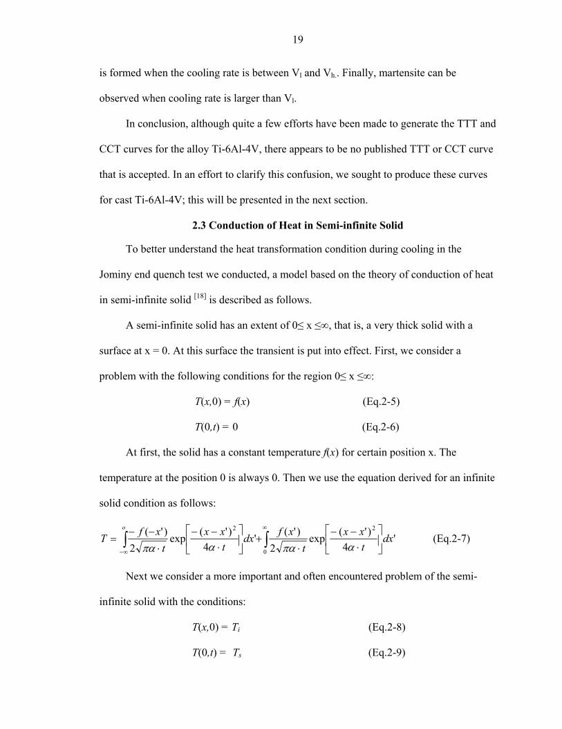
2.3 Conduction of Heat in Semi-infinite Solid
To better understand the heat transformation condition during cooling in the
Jominy end quench test we conducted, a model based on the theory of conduction of heat
in semi-infinite solid [18] is described as follows.
A semi-infinite solid has an extent of 0≤ x ≤∞, that is, a very thick solid with a
surface at x = 0. At this surface the transient is put into effect. First, we consider a
problem with the following conditions for the region 0≤ x ≤∞:
T(x,0) = f(x) (Eq.2-5)
T(0,t) = 0 (Eq.2-6)
At first, the solid has a constant temperature f(x) for certain position x. The
temperature at the position 0 is always 0. Then we use the equation derived for an infinite
solid condition as follows:
'4
)'(exp2
)'('4
)'(exp2
)'( 2
0
2
dxtxx
txfdx
txx
txfT
o
⋅
−−⋅
+
⋅
−−⋅
−−= ∫∫
∞
∞− απααπα (Eq.2-7)
Next we consider a more important and often encountered problem of the semi-
infinite solid with the conditions:
T(x,0) = Ti (Eq.2-8)
T(0,t) = Ts (Eq.2-9)
20
Initially the semi-infinite solid is at a uniform temperature Ti , and its surface is
abruptly brought to a temperature that is maintained at Ts. Thus, we can think of the
temperature field in the vicinity of the surface of a thick solid, even a solid with a finite
thickness.
If we define θ = T- Ti , the conditions become
θ(x,0) = Ti – Ts = θi (Eq.2-10)
θ(0,t) = 0 (Eq.2-11)
Thus Eq.2-7 applies for θ, where f(x´) = θi (uniform initial distribution). We get the
final equation, which is
=
−−
txerf
TTTT
si
s
α2 (Eq.2-12)
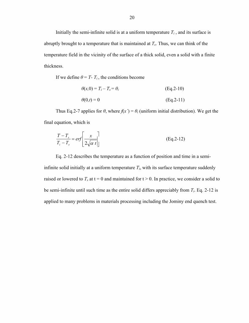
Eq. 2-12 describes the temperature as a function of position and time in a semi-
infinite solid initially at a uniform temperature Ti, with its surface temperature suddenly
raised or lowered to Ts at t = 0 and maintained for t > 0. In practice, we consider a solid to
be semi-infinite until such time as the entire solid differs appreciably from Ti. Eq. 2-12 is
applied to many problems in materials processing including the Jominy end quench test.
CHAPTER 3 EXPERIMENTS
In an effort to fully understand the relationship between the cooling procedures and
microstructures of cast Ti-6Al-4V, we conducted the following experiments. All the Ti-
6Al-4V alloys were supplied by Dr. James Cotton via Dr. James Ault of Precision Cast
Parts.
3.1 Isothermal Heat Treatment Experiments
The typical way to generate a TTT diagram is through isothermal heat treatment
tests. In this study, thin disk-shaped specimens approximately 3mm thick were sectioned
from the 20mm inch diameter cast rods. Small (~1mm diameter) holes were drilled into
the disks near the outer circumference. Wires were then attached to the disks via these
holes. Two salt pots were used initially with the hope that we could avoid oxygen
contamination by heating the samples in air. A set of specimens were first β-solution
treated above 1000°C for 15 minutes in one pot using a Lindberg furnace and then
quickly inserted into the second salt pot for various times at the temperature of interest
for determining the isothermal transformation kinetics and finally removing and
quenching it into water. (Table I)
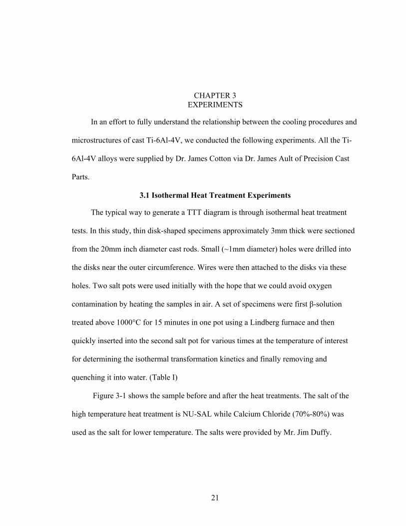
Figure 3-1 shows the sample before and after the heat treatments. The salt of the
high temperature heat treatment is NU-SAL while Calcium Chloride (70%-80%) was
used as the salt for lower temperature. The salts were provided by Mr. Jim Duffy.
21
22
Table 1. Processing, Heat-treatment, Microstructure Summary for Ti-6Al-4V.
Heat Treatment Microstructure Description A 1000°C/30min+750°C/7min+WQ Figure 4-1, 4-6 B 1000°C/30min+750°C/17min+WQ Figure 4-2, 4-9 C 1000°C/30min+830°C/30min+WQ Figure 4-3 D 1000°C/30min+WQ Figure 4-4 D 1000°C/30min+WQ+750°C/10min+WQ Figure 4-5
Before After
Figure 3-1 Samples before and after the isothermal treatments in the salt pots. The “after” sample was lightly ground after heat treatment in order to reach the unaffected region.
3.2 Instrumented Jominy End Quench (JEQ) Experiments
JEQ tests were conducted for the purpose of generation of CCT curves for the Ti-
6Al-4V. For the JEQ experiments, a simple home-made set up (see Figure 3-2) was
constructed using the ASTM A255 specification as a guideline [19].

23
Figure 3-2 Home-made set up for Jominy End Quench test.
A specimen 25mm in diameter and 100 mm in length was cut from a rod-shaped
Ti-6Al-4V casting. One end was ground down to a 600 grit finish while the other end
remained untouched. Four small radial holes were drilled at specific positions (3 mm, 27
mm, 55 mm and 87 mm) from the polished end of the rod and Type K (chromel-alumel)
thermocouples were inserted and fixed into each hole. (See Figure 3-3.) These
thermocouples were connected to a data acquisition system which was used to measure
the temperature-time profile.
The data acquisition system was composed of two cards: an Omega CIO-DAS08
card for A/D conversion and an Omega CIO-EXP16 card which serves as the interface
between the A/D card and the thermocouples.

24
Figure 3-3 Schematic of the Jominy end quench sample instrumented with four thermocouples.
Figure 3-4 Temperature-time data of the JEQ sample in tube furnace (left) were collected
by a data acquisition system (right).
The instrumented 25mm diameter by 100mm long bar sample was wrapped in
fiberfrax, except for the end that would be sprayed with the water, placed in a Lindberg
tube furnace at 1030ºC for 30 minutes, removed with tongs and placed in the JEQ set up.
Water was then turned on and the JEQ experiment was conducted until the temperature of
the opposite end dropped to approximately 140ºC, well below the transus temperature.
25
A
B
Figure 3-5 Sample for the instrumented Jominy end quench test A) before and B) after the test.
Based on the temperature data recorded by the computer, cooling curves for the
different TC positions were plotted. After cooling, the rod was placed into a surface
grinder and parallel flats were ground to about 4mm depth on opposite sides (Figure 3-5
B). This was to make sure that the sample being analyzed had reached the base material
that experienced unidirectional (axial) heat flow and to avoid any α phase caused by
oxidation. On one flat, Rockwell C hardness of the sample was measured with a LECO
hardness tester as a function of distance from the quenched end. The other flat was

26
polished and etched for metallographic analysis. The sample was then sectioned and
polished at the positions where the thermocouples were placed, followed by LOM and
scanning electron microscopy (SEM) examinations. Further transmission electron
microscopy (TEM) analyses were conducted at the spots of thermocouples positions.
3.3 Complementary Continuous Cooling Tests
Since JEQ test can only allow us to examine the final microstructure of the
continuous cooling procedure, to better understand the microstructure transformation at
the elevated temperature, we further conducted some continuous cooling rate tests, in
which samples were first continuous cooled at high temperature after the solution
treatment, then water quenched to room-temperature to eliminate further phase
transformation at low temperature.
In the experiments, a Ti-6Al-4V casting was cut into 3mm thick disk samples. The
samples were then sealed in the evacuated quartz capsules to avoid being oxidized during
heat treatment. After being heated in an air furnace and being held for 30 minutes in the β
field at 1030ºC, the samples were either air cooled or furnace cooled to 900ºC, 800ºC,
700ºC respectively and then water quenched.
3.4 Optical Microscopy
First, optical microscope was used after all the heat treatment tests. The basic
characteristics of the microstructure of the Ti-6Al-4V alloy were determined efficiently
from low magnification to gradually higher magnifications.
All the LOM samples were ground down to 800-grit with SiC polishing paper and
followed by fine polishing using a 0.3µm alumina suspension. Modified Krolls etchant
which is a solution of 2 pct hydrofluoric acid and 6 pct nitric acid was used to chemically
27
etch the mechanically polished specimens. LOM examinations were carried out by a
LECO Neophot 21 optical microscope.
3.5 Scanning Electron Microscopy
For the SEM, a JEOL SEM 6400 equipped with Oxford Link ISIS EDS and Oxford
OPAL electron backscattered secondary electron detector (EBSD) was used.
Samples were mechanically polished down to 0.3µm before SEM examine. Etched
surface was used to form secondary electron images in order to see the grain morphology.
When a backscattered detector was used, unetched surface was examined. Backscattered
electrons images were shown because of the different average atomic number between α
and β (vanadium enrichment) phases. Dot map and line-scan along with the embedded X-
ray techniques were also used in analysis.
3.6 Transmission Electron Microscopy
Thin foils were first cut from the sample by a diamond saw, followed by
mechanical polishing down to about 200µm in thickness with a 600-grit polishing paper.
The 3-mm-diameter disks were punched for further thinning polishing. Samples for TEM
were then prepared using a twin-jet electropolisher at 20 V in a solution bath of 10 pct
perchloric acid and 90 pct methanol. During electropolishing, the temperature of the
electrolytic bath was being kept between -30°C and -40°C. A JEOL TEM200CX
operated at 200kV and a Philips TEM420 equipped with an EDAX EDS system were
used.
CHAPTER 4 RESULTS
Test results come from three different experiments: isothermal heat treatments,
Jominy end quench, and continuous cooling tests. Following sections will present the
microstructures of specimens after these tests.
4.1 Test Results from the Isothermal Heat Treatment
Typical samples before and after the isothermal treatments are shown in Figure 3-1.
As is evident, the samples were somewhat discolored from interactions with the liquid
salts. The initial samples were relatively thin and the attack was so unacceptable that
there might be concerns that the results would be in error. Thus, we started using thicker
specimens so that we were able to grind through the “reaction zone” and sample the base
alloy. It appears that this apparent reaction is actually just dissolution of the alloy into the
salt as opposed to some sort of reaction product. Cross-sections through the thickness of
the samples revealed that the dissolution was greatest along the grain boundaries of the
alloy as might be expected. After working out these issues and identifying suitable
samples, a series of isothermal treatments were performed as described in the previous
chapter.
Optical micrographs from the various samples after these thermal treatments are
shown in Figures 4-1 to 4-5. The initial temperatures, 750ºC and 830ºC, and times, 7, 17,
and 30 minutes, were selected based on the CCT curves that were published by Majdic
and Ziegler where 750ºC was near the proposed “nose” of the curve, while 830ºC was
considerably above the nose.
28
29
In Figure 4-1, the microstructure after 1000ºC 15 min ->750ºC, 7min, WQ has a
number of interesting features. There are apparently nucleation and growth α laths with
an average width of 5µm. The grain boundary of these α laths are somewhat not very
straight. Specifically, there appears to be a film of grain boundary α with the partial
development of sideplates. It is always difficult to identify if the α laths nucleated at
these boundaries or nucleating at some other sites impinged accidentally the boundaries.
However, same microstructure was reported in other work [7]; and by successive
polishings and etchings on the same area, it is confirmed that these sideplates were
nucleated on these grain boundary α layers and grew into the matrix. In addition, there
also appears to be some finer regions coarse α regions in the intergranular regions.
Because the limitation of the optical microscopy, this will be analyzed in greater detail by
SEM and TEM.
For the 750ºC, 17min sample, the microstructure appears similar to the 7 minute
sample (Figure 4-2.), i.e., coarse and fine regions of the α phase. Both the size and the
percentage of the coarse α laths remains the same as the 7 minute sample.
The 830ºC, 30 min sample on the other hand, looked somewhat different. The
former β grain boundaries can no longer be clearly seen. As seen in Figure 4-3., this
structure is slightly coarser and there appears to be some β phase between the α “plates”.
The α grains’ boundary together with the β phase in the α “plates” are relatively straight
comparing to the sample being held at 750ºC.
30
5
(A)
2
(B) Figure 4-1 LOMs of samples after SHT(solution heat-trea
+WQ(water quenched). A) 400x B) 1000x
0 µm
0 µm
tment) + 750ºC for 7 minutes

31
5
(A)
(B) Figure 4-2 LOMs of samples after SHT + 750ºC for 17 m
0 µm
20 µm
inutes +WQ. A) 400x B) 1000x
32
5 (A)
2 (B) Figure 4-3 LOMs of samples after SHT + 830ºC for 30 m
Since these structures are somewhat different from
samples usually reported in the literature, there was some
their evolution. Specifically, there was some concern that
0 µm
0 µm
inutes +WQ. A) 400x B) 1000x
those of continuously cooled
confusion as to the nature of
the β might partially transform
33
to α’ during the quench to 750ºC (and possibly 830ºC). If this is the case, then the TTT
curves can be a bit misleading given that they would represent the decomposition of a
β+α’ structure rather than β decomposition only.
In order to gain insight into this, a sample that was initially 100% α’, obtained by
water quenching from 1000ºC (Figure 4-4), was reheated to 750ºC, held for 30 minutes
and water quenched (Figure 4-5). As can be seen in this figure, the microstructure is quite
different than that in the direct quenched samples. Previous shearing traces, which can be
seen in Figure 4-4 as the very straight lines, can no longer be observed any more. If
compared to the sample that SHT+750ºC 17mins where both finer and coarsened α
regions co-exist, all the α plates in this reheated sample are of very similar size. Some α
plates grow from the boundary.
Since these micrographs are taken at the same magnification as the others, it is
suggested that the apparent “bimodal” distribution of the phases in the previous
isothermal holding specimens must be due to some initial transformation of the β during
the quench followed by further isothermal transformation and coarsening of this partially
transformed structure. Specifically, it is suggested that the sequence for the isothermal
specimen is as follows:
βdirect quench >β+α’isothermal hold >αΝ&G + coarsened α'+ βret
34
2Figure 4-4 LOM of sample SHT + WQ. 1000x
2Figure 4-5 LOM sample SHT + WQ + reheat to 750º
The sample that was SH + 750ºC for 7 minutes
SEM. Figure 4-6 is the secondary electron image of th
the coarse α phase can be seen clearly. However, it is
shearing process took place during the quench from s
0 µm
0 µm
C for 15 minutes.1000x+ WQ was further examined by
e sample. Both shearing traces and
still hard to determine if the
olution temperature 1030ºC to
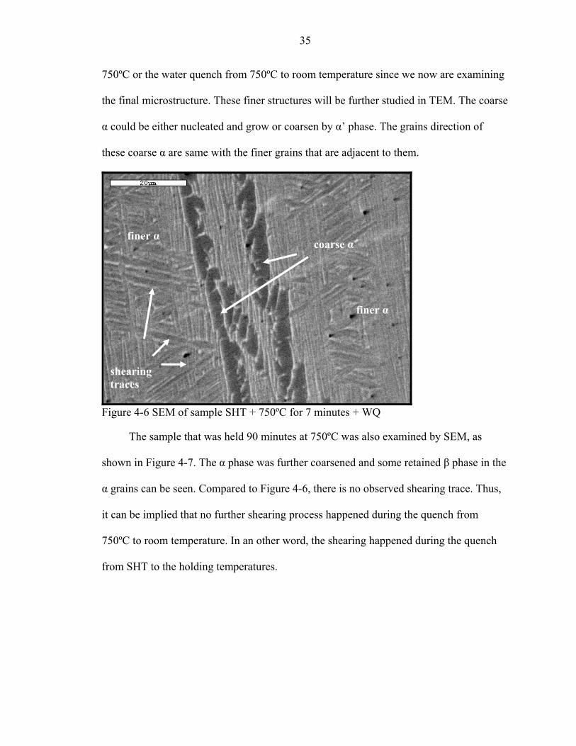
35
750ºC or the water quench from 750ºC to room temperature since we now are examining
the final microstructure. These finer structures will be further studied in TEM. The coarse
α could be either nucleated and grow or coarsen by α’ phase. The grains direction of
these coarse α are same with the finer grains that are adjacent to them.
finer α coarse α
finer α
Fi
sh
α
it
75
fro
shearingtraces
gure 4-6 SEM of sample SHT + 750ºC for 7 minutes + WQ
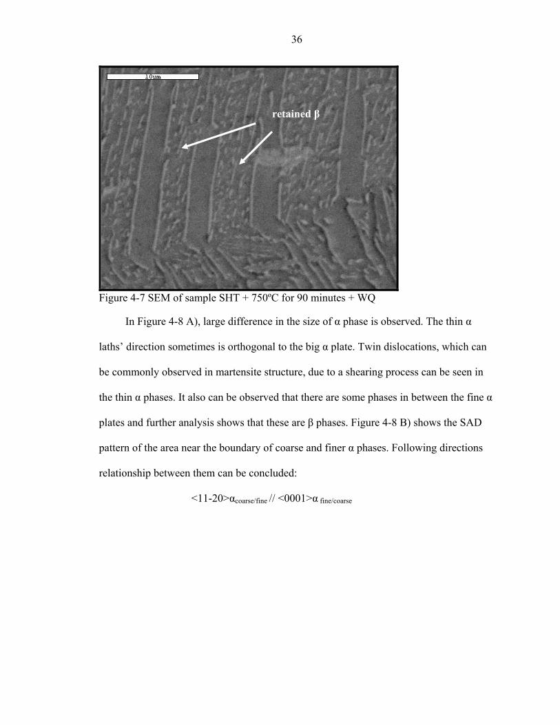
The sample that was held 90 minutes at 750ºC was also examined by SEM, as
own in Figure 4-7. The α phase was further coarsened and some retained β phase in the
grains can be seen. Compared to Figure 4-6, there is no observed shearing trace. Thus,
can be implied that no further shearing process happened during the quench from
0ºC to room temperature. In an other word, the shearing happened during the quench
m SHT to the holding temperatures.
36
retained β
Figure 4-7 SEM of sample SHT + 750ºC for 90 minutes + WQ
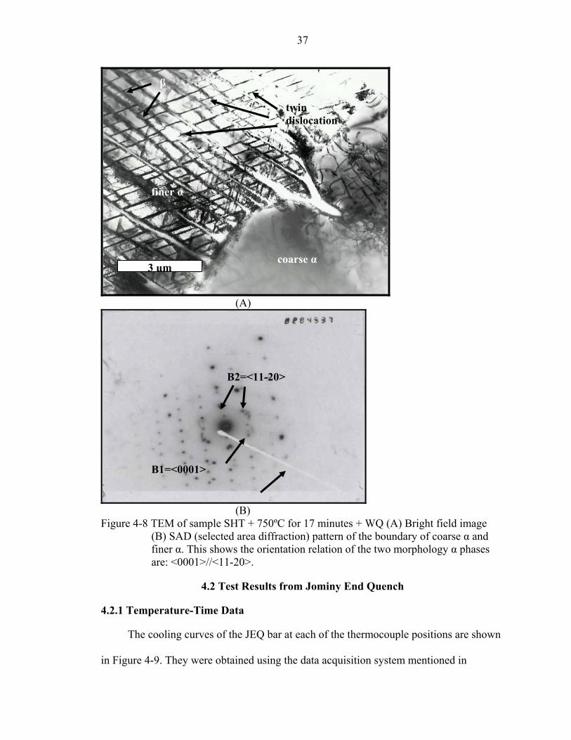
In Figure 4-8 A), large difference in the size of α phase is observed. The thin α
laths’ direction sometimes is orthogonal to the big α plate. Twin dislocations, which can
be commonly observed in martensite structure, due to a shearing process can be seen in
the thin α phases. It also can be observed that there are some phases in between the fine α
plates and further analysis shows that these are β phases. Figure 4-8 B) shows the SAD
pattern of the area near the boundary of coarse and finer α phases. Following directions
relationship between them can be concluded:
<11-20>αcoarse/fine // <0001>α fine/coarse
37
β
finer α
coarse α 3
Figure 4-8
4.2.1 Temp
The c
in Figure 4
µm
(A)
B2=<11-20>
B1=<0001>
(B) TEM of sample SHT + 750ºC (B) SAD (selected area diffracfiner α. This shows the orientaare: <0001>//<11-20>.
4.2 Test Results fr
erature-Time Data
ooling curves of the JEQ bar a
-9. They were obtained using t
twin dislocation
for 17 minutes + WQ (A) Bright field image tion) pattern of the boundary of coarse α and tion relation of the two morphology α phases
om Jominy End Quench
t each of the thermocouple positions are shown
he data acquisition system mentioned in

38
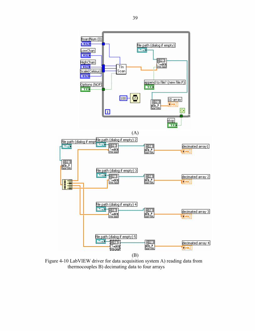
Chapter 3, with the temperature sampling rate at each thermocouple being 10 times/sec.
As seen in the figure, the temperature at 3mm dropped at a very high rate whereas the
cooling at 55mm and 87mm are slow. A LabVIEW driver program is designed especially
for controlling of the A/D card, the extension card, and the sampling action (Figure 4-10
A). Figure 4-10 B) is the LabVIEW program to decimate the data, that had been collected
by the previous program, to each channel and save as a format that can be read by other
program, e.g. Excel or Matlab.
100
101
102
103
0
200
400
600
800
1000
1200
Log time (sec)
Tem
para
ture
(C)
Cooling Curves
AB C
D
A: 3mmB: 27mmC: 55mmD: 87mm
Figure 4-9 Experimental cooling curves from K-type thermocouples embedded in the
JEQ sample. (3mm, 27mm, 55mm and 87mm from the quench end)
39
(A)
(B)
Figure 4-10 LabVIEW driver for data acquisition system A) reading data from thermocouples B) decimating data to four arrays
40
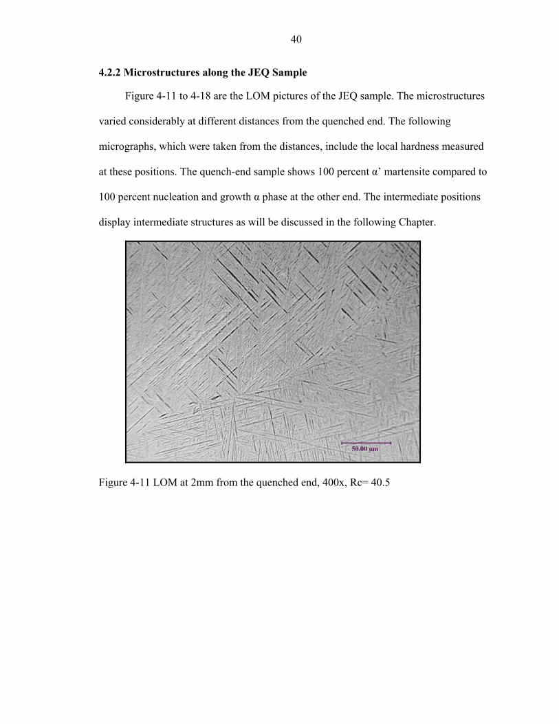
4.2.2 Microstructures along the JEQ Sample
Figure 4-11 to 4-18 are the LOM pictures of the JEQ sample. The microstructures
varied considerably at different distances from the quenched end. The following
micrographs, which were taken from the distances, include the local hardness measured
at these positions. The quench-end sample shows 100 percent α’ martensite compared to
100 percent nucleation and growth α phase at the other end. The intermediate positions
display intermediate structures as will be discussed in the following Chapter.
Figure 4-11 LOM at 2mm from the quenched end, 400x, Rc= 40.5
41
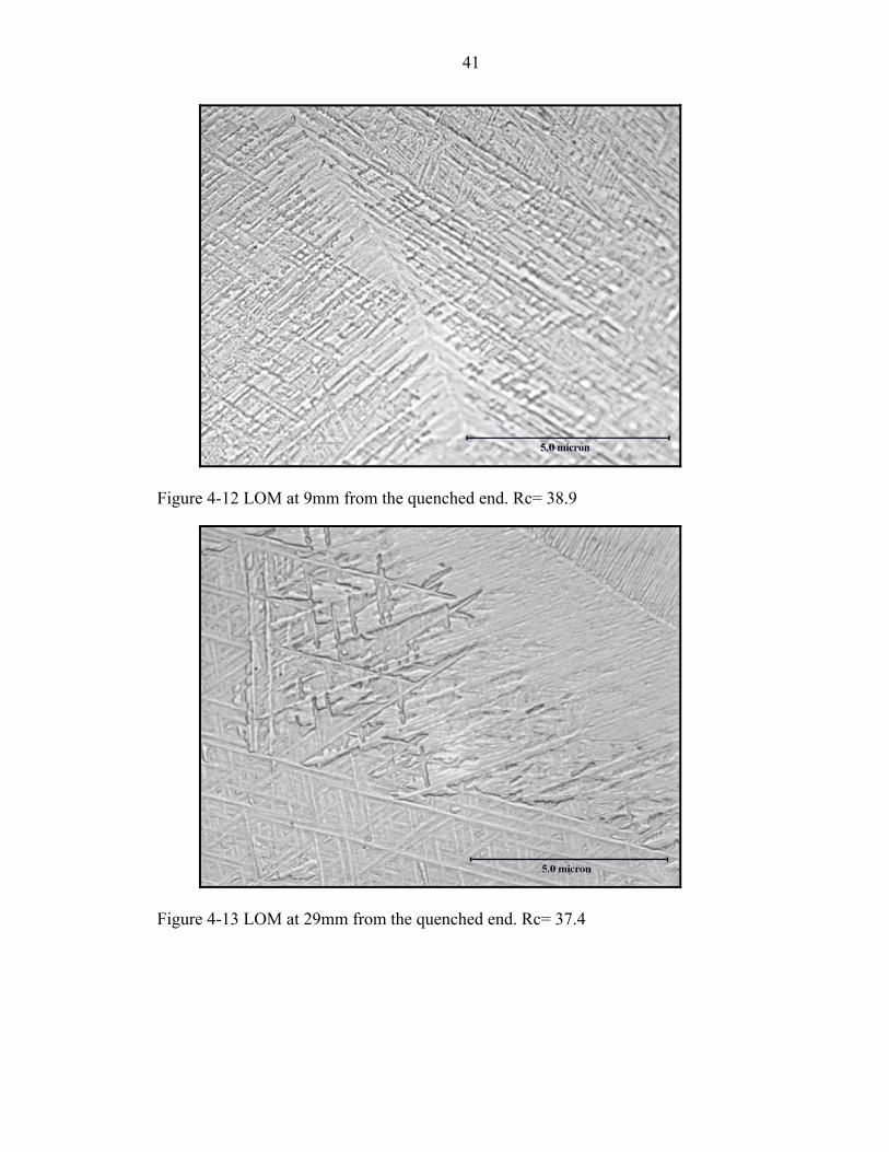
Figure 4-12 LOM at 9mm from the quenched end. Rc= 38.9
Figure 4-13 LOM at 29mm from the quenched end. Rc= 37.4
42
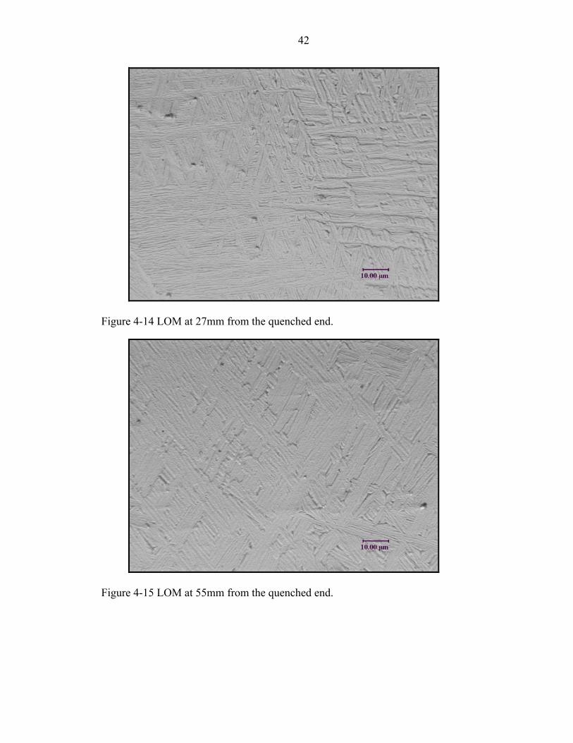
Figure 4-14 LOM at 27mm from the quenched end.
Figure 4-15 LOM at 55mm from the quenched end.

43
Figure 4-16 LOM at 66mm from the quenched end. Rc= 36.2
prior β grain boundary
Figure 4-17 LOM at 75mm from the quenched end. Rc= 36.8
44
prior β grain boundary
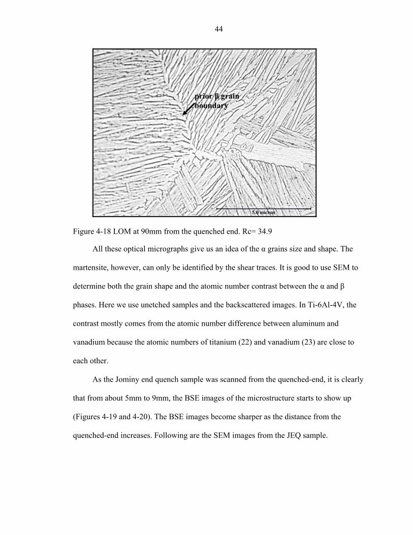
Figure 4-18 LOM at 90mm from the quenched end. Rc= 34.9
All these optical micrographs give us an idea of the α grains size and shape. The
martensite, however, can only be identified by the shear traces. It is good to use SEM to
determine both the grain shape and the atomic number contrast between the α and β
phases. Here we use unetched samples and the backscattered images. In Ti-6Al-4V, the
contrast mostly comes from the atomic number difference between aluminum and
vanadium because the atomic numbers of titanium (22) and vanadium (23) are close to
each other.
As the Jominy end quench sample was scanned from the quenched-end, it is clearly
that from about 5mm to 9mm, the BSE images of the microstructure starts to show up
(Figures 4-19 and 4-20). The BSE images become sharper as the distance from the
quenched-end increases. Following are the SEM images from the JEQ sample.
45
Figure 4-19 BSE of unetched sample of 5mm away from JEQ end, 1500x
Figure 4-20 BSE of unetched sample of 9mm away from JEQ end, 1500x

46
Figure 4-21 BSE of unetched sample of 12mm away from JEQ end, 1500x
Figure 4-22 BSE of unetched sample of 16mm away from JEQ end, 1500x
47
Figure 4-23 BSE of unetched sample of 25.6mm away from JEQ end, 1500x
Figure 4-24 BSE of unetched sample of 29mm away from JEQ end, 1500x
48
Figure 4-25 BSE of unetched sample of 52mm away from JEQ end, 1500x
Figure 4-26 BSE of unetched sample of 66mm away from JEQ end, 1500x
49
Figure 4-27 BSE of unetched sample of 85mm away from JEQ end, 1500x
Figure 4-28 BSE of unetched sample of 86mm away from JEQ end, 1500x
Along with the SEM examination, TEM was also conducted near the
thermocouples were located. Figure 4-29 is from the JEQ sample’s quenched end. The
50
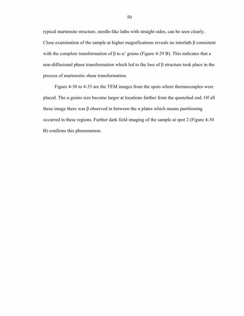
typical martensite structure, needle-like laths with straight sides, can be seen clearly.
Close examination of the sample at higher magnifications reveals no interlath β consistent
with the complete transformation of β to α’ grains (Figure 4-29 B). This indicates that a
non-diffusional phase transformation which led to the loss of β structure took place in the
process of martensitic shear transformation.
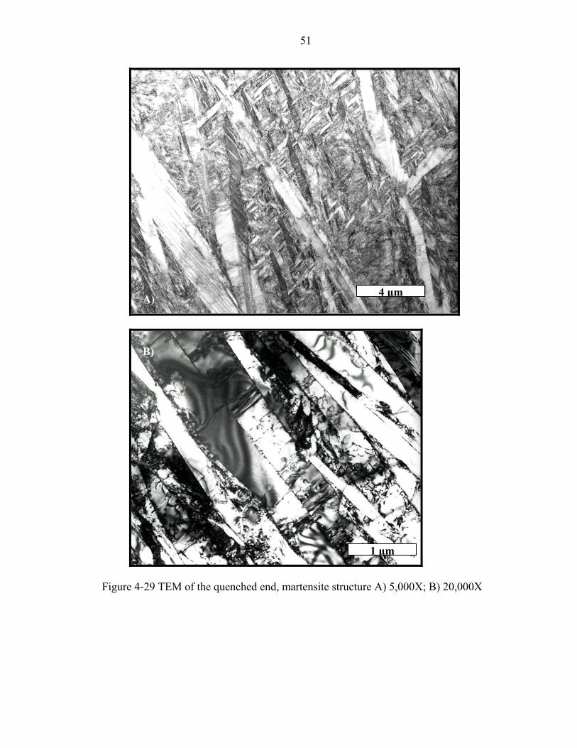
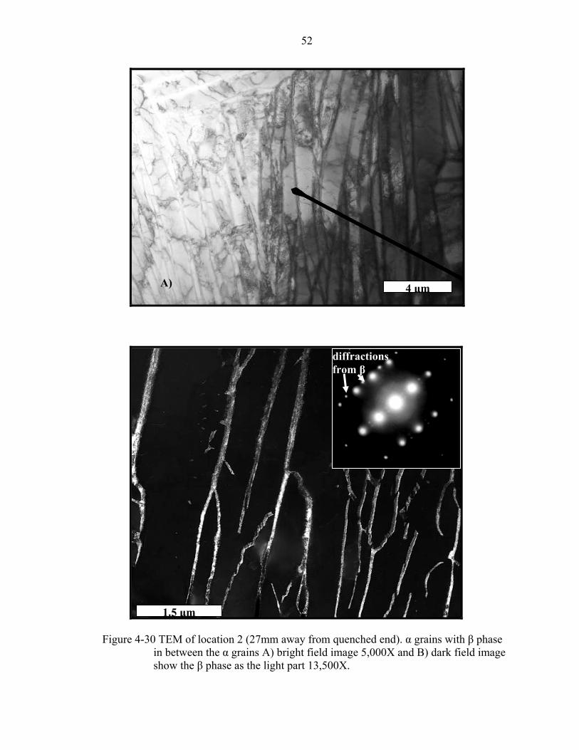
Figure 4-30 to 4-33 are the TEM images from the spots where thermocouples were
placed. The α grains size become larger at locations farther from the quenched end. Of all
these image there was β observed in between the α plates which means partitioning
occurred in these regions. Further dark field imaging of the sample at spot 2 (Figure 4-30
B) confirms this phenomenon.
51
4A) B)
1
Figure 4-29 TEM of the quenched end, martensite structure
µm
A
µm
) 5,000X; B) 20,000X
52
A) B)
4
diffractions from β
1
Figure 4-30 TEM of location 2 (27mm away from quenched end). αin between the α grains A) bright field image 5,000X anshow the β phase as the light part 13,500X.
µm
.5 µm
grains with β phase d B) dark field image

53
4
Figure 4-31 TEM of location 3 (55mm away from quenched end) α grains grows at different directions 5,000X
β
α
β
1
Figure 4-32 TEM of location 3 (55mm away from quenched end)different directions with β phase in between the α-α gr
µm
µm
α grains grows at ain boundary 20,000X
54
Figure 4-33 TEM of location 4 (87mm away from quenched end) more coarsened α
grains 3,000X
10 µm
4.2.3 Rockwell C Hardness Data
After the test, two parallel flats were ground to 4mm in depth. Rockwell C hardness
was measured on one flat. Figure 4-34 is the hardness vs. distance from the quenched-
end. Two samples were heated and end quenched under the same condition and the
hardness results were consistent. The hardness near the quenched end is somewhat higher
and decreases with distance from the quenched end. This is probably due to the finer α’ in
this region. However, the hardness differences are relatively minor.

55
Hardness vs. Distance for Cast Ti-6Al-4V
26
28
30
32
34
36
38
40
42
0 20 40 6Distance from quenched end in milimeter
Rock
wel
l C h
ardn
ess
is s
cale
0
A)
Hardness vs. Distance for Cast Ti-6Al-4V
26
28
30
32
34
36
38
40
42
0 20 40 60 80 100 120Distance from quenched end in milimeter
Rock
wel
l C h
arne
ss s
cale
B) Figure 4-34 Hardness vs. position for the Ti-6Al-4V JEQ specimens from two same A)
and B) conditions test.
56
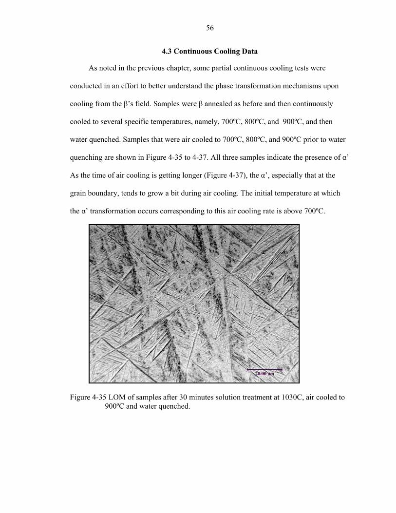
4.3 Continuous Cooling Data
As noted in the previous chapter, some partial continuous cooling tests were
conducted in an effort to better understand the phase transformation mechanisms upon
cooling from the β’s field. Samples were β annealed as before and then continuously
cooled to several specific temperatures, namely, 700ºC, 800ºC, and 900ºC, and then
water quenched. Samples that were air cooled to 700ºC, 800ºC, and 900ºC prior to water
quenching are shown in Figure 4-35 to 4-37. All three samples indicate the presence of α’
As the time of air cooling is getting longer (Figure 4-37), the α’, especially that at the
grain boundary, tends to grow a bit during air cooling. The initial temperature at which
the α’ transformation occurs corresponding to this air cooling rate is above 700ºC.
Figure 4-35 LOM of samples after 30 minutes solution treatment at 1030C, air cooled to 900ºC and water quenched.
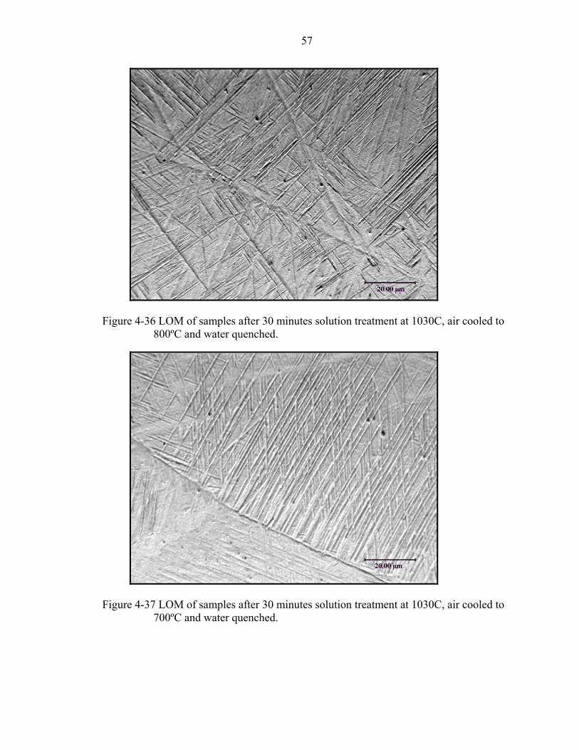
57
Figure 4-36 LOM of samples after 30 minutes solution treatment at 1030C, air cooled to 800ºC and water quenched.
Figure 4-37 LOM of samples after 30 minutes solution treatment at 1030C, air cooled to 700ºC and water quenched.
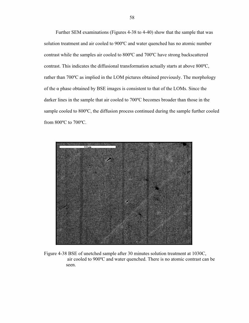
58
Further SEM examinations (Figures 4-38 to 4-40) show that the sample that was
solution treatment and air cooled to 900ºC and water quenched has no atomic number
contrast while the samples air cooled to 800ºC and 700ºC have strong backscattered
contrast. This indicates the diffusional transformation actually starts at above 800ºC,
rather than 700ºC as implied in the LOM pictures obtained previously. The morphology
of the α phase obtained by BSE images is consistent to that of the LOMs. Since the
darker lines in the sample that air cooled to 700ºC becomes broader than those in the
sample cooled to 800ºC, the diffusion process continued during the sample further cooled
from 800ºC to 700ºC.
Figure 4-38 BSE of unetched sample after 30 minutes solution treatment at 1030C, air cooled to 900ºC and water quenched. There is no atomic contrast can be seen.

59
Figure 4-39 BSE of unetched samples after 30 minutes solution treatment at 1030ºC, air cooled to 800ºC and water quenched. The atomic contrast can be seen as the thin dark lines.
Figure 4-40 BSE of unetched samples after 30 minutes solution treatment at 1030ºC, air cooled to 700ºC and water quenched. The dark lines were broader than those in Figure 4-39.
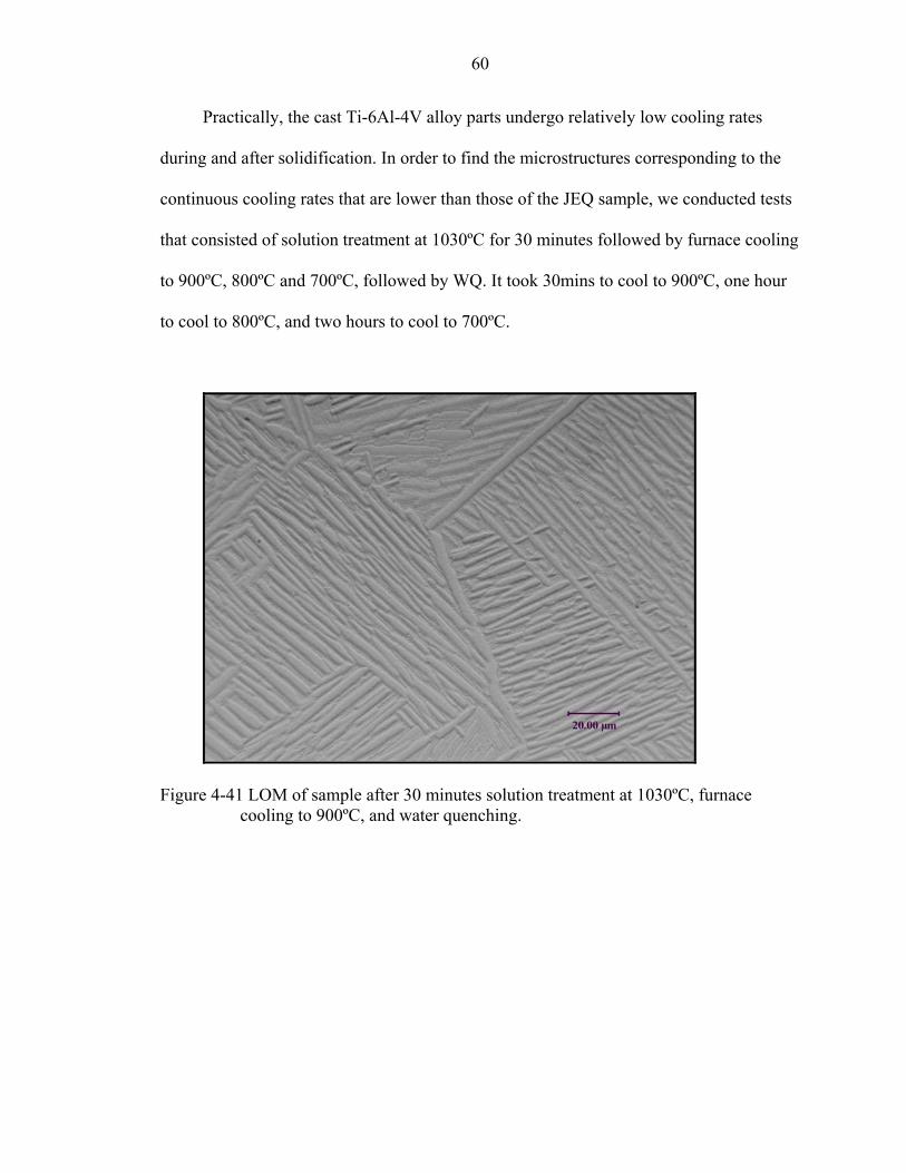
60
Practically, the cast Ti-6Al-4V alloy parts undergo relatively low cooling rates
during and after solidification. In order to find the microstructures corresponding to the
continuous cooling rates that are lower than those of the JEQ sample, we conducted tests
that consisted of solution treatment at 1030ºC for 30 minutes followed by furnace cooling
to 900ºC, 800ºC and 700ºC, followed by WQ. It took 30mins to cool to 900ºC, one hour
to cool to 800ºC, and two hours to cool to 700ºC.
Figure 4-41 LOM of sample after 30 minutes solution treatment at 1030ºC, furnace cooling to 900ºC, and water quenching.
61
Figure 4-42 LOM of sample after 30 minutes solution treatment at 1030ºC, furnace cooling to 800ºC, and water quenching.
Figure 4-43 LOM of sample after 30 minutes solution treatment at 1030ºC, furnace cooling to 700ºC, and water quenching.

62
Figures 4-44 to 4-46 are the BEIs of samples that were solution treated at 1030ºC,
furnace cooled to 900ºC, 800ºC, 700ºC, and water quenched. The α phase grows bigger
when furnace cooling time is longer. Meanwhile, the β phase continuously shrinks, as
shown in the SEM picture in which the percentage of high average atomic number phase
(light part) becomes smaller. An acicular α structure dominates under all three furnace
cooling conditions, which means that the shearing process is totally depressed.
Figure 4-44 BSE of sample after 30 minutes solution treatment at 1030ºC, furnace cooling to 900ºC and water quenching

63
Figure 4-45 BSE of samples after 30 minutes solution treatment at 1030ºC, furnace cooling to 800ºC and water quenching.
Figure 4-46 BSE of samples after 30 minutes solution treatment at 1030ºC, furnace cooling to 700ºC and water quenching.

CHAPTER 5 ANALYSIS AND DISCUSSIONS
In this chapter, we will present some analysis based on the test results of the
previous chapter. Section one is the theory of the simulation of the cooling rates of JEQ
sample. Then, a CCT curve for Ti-6Al-4V is presented in section two. The growth
directions of the α laths of different cooling rates are discussed in section three. Finally,
some ideas for generating TTT curves are given in section four.
5.1 Simulation of the Cooling Rates of Jominy End Quench Sample
The cooling curves of the JEQ bar at each of the thermocouple positions are shown
in Figure 4-10. They were obtained using the data acquisition system constructed for this
study, and sampling the temperature of each thermocouple at a rate of 10 times/sec. Since
only limited number of positions in the JEQ bar can be monitored experimentally, it is
useful to predict the temperature-time behavior at any position that we are interested in
on the JEQ bar. To simulate the end-quench procedure, we used a simple one-
dimensional heat flow model that is based on semi-infinite solid heat transfer
conditions[17]. In this model, the relationship of the real time temperature T and time t at a
certain spot of the JEQ bar is represented as:
=
−−
txerf
TTTT
si
s
α2 (Eq. 5-1)
where Ti is the initial temperature of the bar, which in this case, is the solution
treatment temperature 1030ºC; Ts the quenched end surface temperature, which in this
64
65
case, is the water temperature (25ºC); x the distance from the cooling end; and α the
thermal diffusivity of the material given by:
pC
k⋅
=ρ
α (Eq. 5-2)
The constants in Eq. 5-2 are k thermal conductivity, Cp the heat capacity, and ρ the
density. Table 2 shows these physical properties of Ti-6Al-4V and a Carbon Steel for
comparison.
Table 2. Physical Properties of Ti-6Al-4V and a Carbon Steel [20] Materials ρ (kg•m-3) k (W•m-1
•K-1) Cp (J• kg-1 •K-1) α(W•m2•J-1)
Ti-6Al-4V 4430 6.6 580 2.5 x 10⁻⁶ Steel (Fe 85.37%) 7850 15 450 4.2 x 10⁻⁶
The cooling rate at some position x to the quenched end and at time t can be
obtained by taking the derivative of T with respect to t:
tx
is et
xTTtT α
πα4
3
2
2)(
−
⋅⋅−=∂∂ (Eq. 5-3)
The calculated cooling curves for the JEQ bar obtained using this model and the
experimental cooling curves from the JEQ test are shown in Figure 5-1 (A) and (B),
respectively. It can be seen that the calculated curves of the part near the quenched end
(in this test, at the position about 30-40mm from the quenched end) are comparable to the
experimental curves whereas the agreement is much poorer at larger distances from the
quenched end (more than 40mm away). At locations farther than 40mm from the
quenched end, the calculated rates are considerably lower than the experimental cooling
rates; this is not surprising given that the sample is not an ideal semi-infinite solid with
one end maintained at the temperature of the solution treatment while the other end is
66
quenched. Rather, the whole specimen underwent simultaneous air cooling during the
end quench experiment. For steel, which has almost a 2 times increasing in thermal
diffusivity (α), this same model is expected to be accurately for the first 15mm from the
quenched end [17]. Specifically, since the thermal diffusivity of Ti-6Al-4V is about 2
times lower than that of the steel, which means the less heat flow other than semi-infinite
flow for Ti-6Al-4V than for steel, this ideal semi-infinite model can actually simulate a
longer distance from quench end than it does on steel. In this case, the calculated cooling
curves can be used to represent the actual cooling condition on the JEQ bar within the
distance of 40mm from the quenched end which is quite enough, considering the
microstructures that are farther than this distance do change fundamentally which will be
described in the following CCT curves.
Based on the calculated cooling curves obtained above, the cooling rates for
specific distances from the quenched end were derived as shown in Table 3.
Table 3. Cooling Rates at some Interested Spots along JEQ Sample Distance from quenched end (mm) Calculated Cooling Rate (Cº/s) 2mm >1000 5mm ~150 9mm ~50 19mm ~20 24mm ~5 28mm ~3 50mm <1.25

67
100 101 102 103 104 1050
200
400
600
800
1000
1200 Calculated Cooling Curves
Log Time (SEC)
Tem
pera
ture
(o C)
1:1mm2:11mm3:21mm4:31mm5:41mm6:51mm7:61mm8:71mm9:81mm10:91mm
1
2 3
4 5 6 7 8 9 10
A)
100
101
102
103
0
200
400
600
800
1000
1200
Log Time (SEC)
Tem
pera
ture
(o C)
JEQ Test Cooling Curves
A: 3mm B: 27mmC: 55mmD: 87mm
A
B C
D
B)
Figure 5-1 Cooling curves of JEQ sample A) calculated cooling curves using the semi-infinite solid heat transfer model; B) experimental cooling curves acquired from temperature data acquisition system during the JEQ test
68
5.2 CCT Curves for Ti-6Al-4V
Based on the analysis of the SEM and LOM pictures of the JEQ samples, a CCT
curve was constructed (Figure 5-2). First of all, Ti-6Al-4V alloy when is continuously
cooled from above the β transus at rates higher than 150ºC/s, 0 percent partitionless
martensite α’ is formed. When cooled from β solution at a rate between ~150ºC/s and
~3ºC/s, a mixture of shear, N&G α, and retained β phase is formed through the process of
diffusional transformations with partial participation of diffusionless (shearing). When
the Ti-6Al-4V alloy is cooled slower than ~3ºC/s, only N&G α and retained β are formed
through pure nucleation and diffusional growth processes.
The amount of solute partitioning was estimated from the BSE images-when no Z
contrast was observed, it was assumed that no partitioning had occurred. As the CCT
curves (Figure 5-2) reflect this behavior, i.e., as the cooling rate (distance from the
quenched end) is decreased, the percent displacive transformation decreases from 100%
α’ (cooling rate >150ºC/s) to 0% α’ (cooling rate <~3ºC/s). Similar behavior has been
suggested for Ti3Al + Nb alloys [21].
When analyzing the SEM picture, we think that the contrast in the BSE image
indicates the incidence of element jump between α and β, in other words, the incidence of
diffusion growth of α phase. However, we didn’t include some special conditions under
which diffusion and growth happen coincidently so that the concentrations of alloying
elements are remaining the same, e.g. massive transformation [22]. This is a quite special
condition and hard to tell.
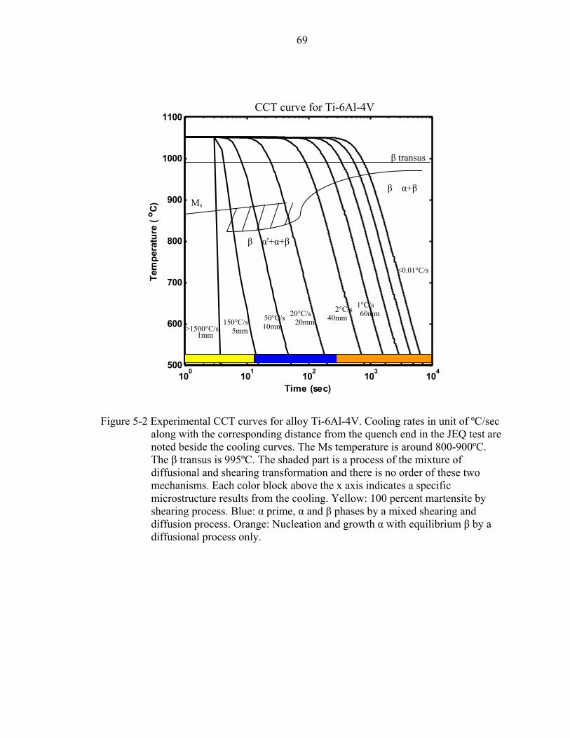
69
100 101 102 103 104500
600
700
800
900
1000
1100
Time (sec)
Tem
pera
ture
(o C
)β transus
>1500°C/s150°C/s 50°C/s 20°C/s 2°C/s 1°C/s
<0.01°C/s
Ms
β α+β
β α'+α+β
10mm5mm1mm
20mm 40mm 60mm
CCT curve for Ti-6Al-4V
Figure 5-2 Experimental CCT curves for alloy Ti-6Al-4V. Cooling rates in unit of ºC/sec along with the corresponding distance from the quench end in the JEQ test are noted beside the cooling curves. The Ms temperature is around 800-900ºC. The β transus is 995ºC. The shaded part is a process of the mixture of diffusional and shearing transformation and there is no order of these two mechanisms. Each color block above the x axis indicates a specific microstructure results from the cooling. Yellow: 100 percent martensite by shearing process. Blue: α prime, α and β phases by a mixed shearing and diffusion process. Orange: Nucleation and growth α with equilibrium β by a diffusional process only.
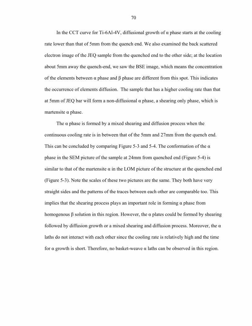
70
In the CCT curve for Ti-6Al-4V, diffusional growth of α phase starts at the cooling
rate lower than that of 5mm from the quench end. We also examined the back scattered
electron image of the JEQ sample from the quenched end to the other side; at the location
about 5mm away the quench-end, we saw the BSE image, which means the concentration
of the elements between α phase and β phase are different from this spot. This indicates
the occurrence of elements diffusion. The sample that has a higher cooling rate than that
at 5mm of JEQ bar will form a non-diffusional α phase, a shearing only phase, which is
martensite α phase.
The α phase is formed by a mixed shearing and diffusion process when the
continuous cooling rate is in between that of the 5mm and 27mm from the quench end.
This can be concluded by comparing Figure 5-3 and 5-4. The conformation of the α
phase in the SEM picture of the sample at 24mm from quenched end (Figure 5-4) is
similar to that of the martensite α in the LOM picture of the structure at the quenched end
(Figure 5-3). Note the scales of these two pictures are the same. They both have very
straight sides and the patterns of the traces between each other are comparable too. This
implies that the shearing process plays an important role in forming α phase from
homogenous β solution in this region. However, the α plates could be formed by shearing
followed by diffusion growth or a mixed shearing and diffusion process. Moreover, the α
laths do not interact with each other since the cooling rate is relatively high and the time
for α growth is short. Therefore, no basket-weave α laths can be observed in this region.
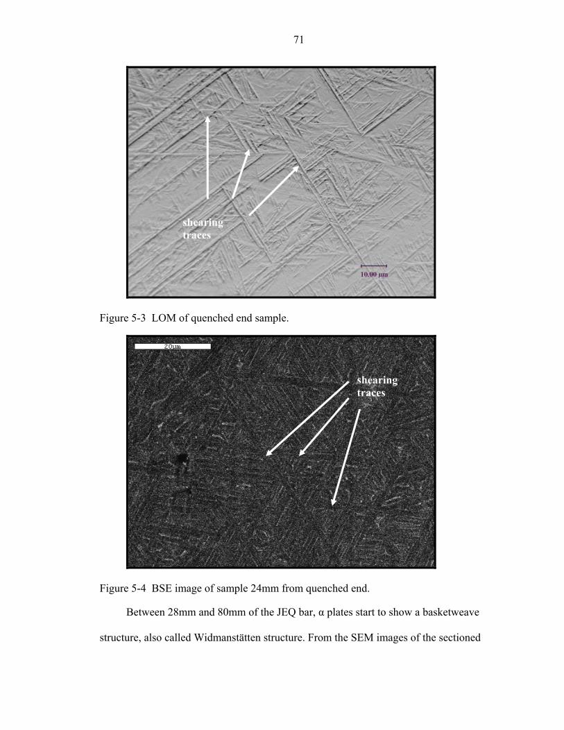
71
Figure 5-3 LOM of quenched end sample.
Figure 5-4 BSE image of sample 24mm from quenched en
Between 28mm and 80mm of the JEQ bar, α plates s
structure, also called Widmanstätten structure. From the SE
shearingtraces
shearingtraces
d.
tart to show a basketweave
M images of the sectioned
72
surfaces in this region (Figure 4-25 and 4-26), some α plates were intercepted by other α
plates which have different growth orientations. It is believed that this is due to the
interaction of contiguous α-plates during their growth. Compared to the much slower
cooling area that is farther than 80mm from quenched end, the nucleation rate in this area
is relatively high because of the supersaturated condition. It turns out that the number of
nuclei at the very early stage of cooling is relatively large so that when they grow, they
tend to interact with each other because of the limited space left.
In Figure 4-29, the sample from 86mm and farther from the quenched end shows
acicular α phase with β phase in between the α grains. Comparing the structure to that of
80mm from quenched end, we discover there are almost no α plates interlaced with each
other, which indicates no α plates interacted with each other during their growth. It is
believed that the relatively small cooling rate and low nucleation rate are the reasons for
this phenomenon. Since fewer nuclei formed during the early stages of the continuous
cooling, the nucleated α have enough space to grow without contact with other α laths
nearby. During the cooling process, the remaining β continuously shrinks while the
nucleated α continuously grows.
The Ms is believed to be very high, between 800ºC and 900ºC, as indicated in the
continuous cooling tests in which samples were air cooled to 900ºC, 800ºC and 700ºC,
after 30 minute solution treatments, and then water quenched. In the LOM picture
(Figures 4-37 to 4-39), all of them show the characteristic martensitic α’ morphology.
The traces of shearing are clear. However, in the BSE images of un-etched samples
(Figures 4-40 to 4-42), the samples that were air cooled to 900ºC showed no significant
compositional variation in the α and β phases, while the sample air cooled to 800ºC
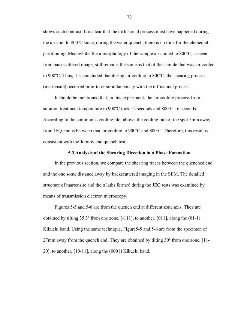
73
shows such contrast. It is clear that the diffusional process must have happened during
the air cool to 800ºC since, during the water quench, there is no time for the elemental
partitioning. Meanwhile, the α morphology of the sample air cooled to 800ºC, as seen
from backscattered image, still remains the same as that of the sample that was air cooled
to 900ºC. Thus, it is concluded that during air cooling to 800ºC, the shearing process
(martensite) occurred prior to or simultaneously with the diffusional process.
It should be mentioned that, in this experiment, the air cooling process from
solution treatment temperature to 900ºC took ~2 seconds and 800ºC ~6 seconds.
According to the continuous cooling plot above, the cooling rate of the spot 5mm away
from JEQ-end is between that air cooling to 900ºC and 800ºC. Therefore, this result is
consistent with the Jominy end quench test.
5.3 Analysis of the Shearing Direction in α Phase Formation
In the previous section, we compare the shearing traces between the quenched end
and the one some distance away by backscattered imaging in the SEM. The detailed
structure of martensite and the α laths formed during the JEQ tests was examined by
means of transmission electron microscopy.
Figures 5-5 and 5-6 are from the quench end at different zone axis. They are
obtained by tilting 35.3º from one zone, [-111], to another, [011], along the (01-1)
Kikuchi band. Using the same technique, Figure5-5 and 5-6 are from the specimen of
27mm away from the quench end. They are obtained by tilting 30º from one zone, [11-
20], to another, [10-11], along the (0001) Kikuchi band.

74
2 µm
[01ī]
[110]
Figure 5-5 TEM micrograph and the corresponding electron diffraction patterns for the quenched end at B=<111> of prior β. The directions of some needle like grains were analyzed.
Trace analysis of the martensite and the α laths are shown in Figure 5-7. In order to
get the true directions of the traces interesting, for each sample, two BF and
corresponding SAD images from different beam directions were captured so that two
projection directions of a feature were known. By combining the two projection
directions of each feature, the true direction can be derived. After calculating the true
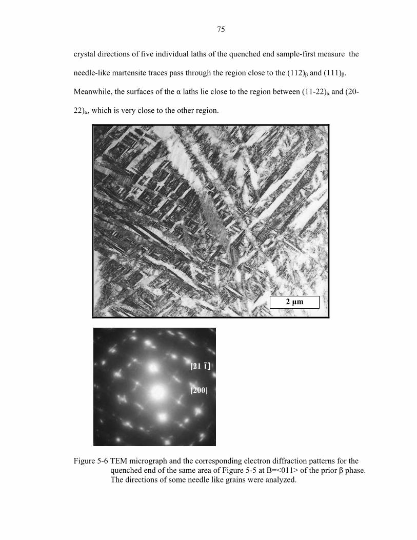
75
crystal directions of five individual laths of the quenched end sample-first measure the
needle-like martensite traces pass through the region close to the (112)β and (111)β.
Meanwhile, the surfaces of the α laths lie close to the region between (11-22)α and (20-
22)α, which is very close to the other region.
2 µm
[21 ī]
[200]
Figure 5-6 TEM micrograph and the corresponding electron diffraction patterns for the quenched end of the same area of Figure 5-5 at B=<011> of the prior β phase. The directions of some needle like grains were analyzed.
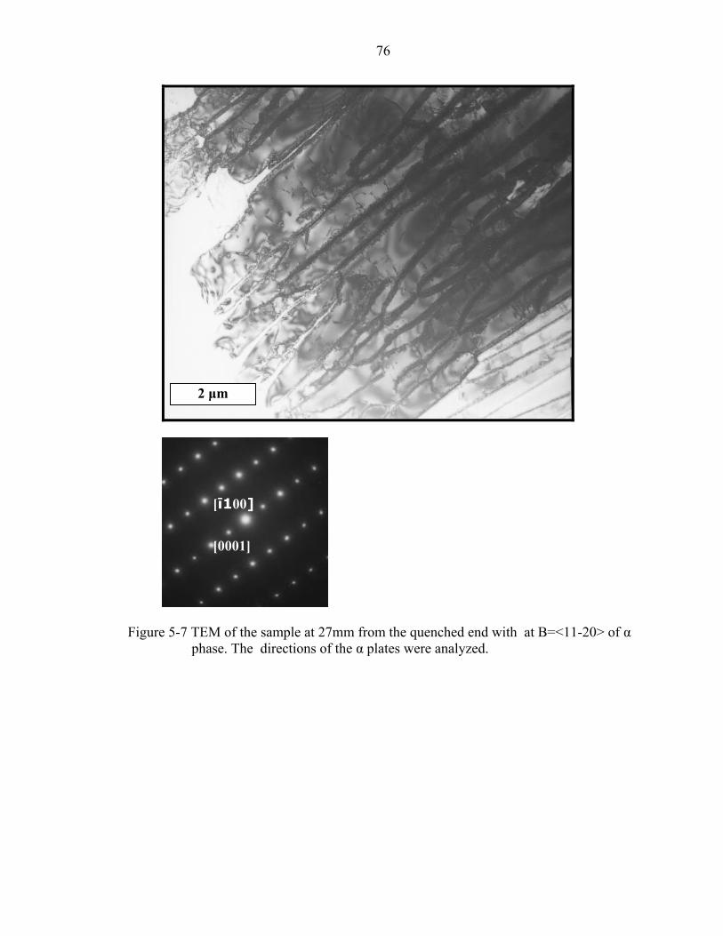
76
2 µm
[ī100]
[0001]
Figure 5-7 TEM of the sample at 27mm from the quenched end with at B=<11-20> of α phase. The directions of the α plates were analyzed.
77
2 µm
[ī2ī0]
[0002]
Figure 5-8 TEM of the sample at 27mm from the quenched end of the same area of Figure 5-7 at B=<10-10> of α phase. The directions of the α plates were analyzed.

78
Figure 5-9 Stereographic analysis shows the relationship between the Amartensite needle-like laths lies in the circled region, and B)traces of the α laths lies in the regions that circled.
A)
B)
) directions of directions of

79
5.4 TTT Curve for Ti-6Al-4V
As have discussed in Chapter 2, considerable efforts have been spent in plotting the
TTT curve for Ti-6Al-4V. The common conclusion of all the presented TTT curves is
that the incubation time of the α phase is very short, less than several seconds. This may
be the case. The real reason, however, might be the following. Since the Martensite
temperature is so high, when a sample is quenched to a certain isothermal temperature,
martensite α’ phase has already formed; the subsequent isothermal holding allows the
growth and coarsening of the α phase. Since the martensite α’ structure can be quickly
coarsened by diffusional process, the incubation time for the N&G α phase seems to be
very short.
In the entire isothermal tests we conducted, the solution β seemed to have totally
transformed to α phase after being held at a certain temperature and before water quench
to room temperature. If there is any solution β left at the end of isothermal holding, these
β phase should transform to martensite during the water quench. Therefore, the resulting
structure should look like partial nucleation and growth α, and partial martensitic α’. By
calculating the percentage of the non-martensite α phase, we know the percentage of the
transformed α. However, after analysis the isothermal samples, no α’ was observed.
Thus, the solution β may have already partially transformed to martensite during the
quench from solution temperature to the holding temperature. The holding makes the
martensite coarsen so that the resulting structure is formed.
CHAPTER 6 CONCLUSION
This project is aimed at generation of TTT and CCT curves of cast Ti-6Al-4V alloy
which is essential to controlling the microstructures in Ti-6Al-4V. We conducted the
isothermal test for TTT curves and the Jominy end quench test for the CCT curves.
Continuous cooling tests were also conducted, in an effort to better understand the
mechanism of the phase transformation during the cooling. After the experiments, we
plotted CCT curves. In addition, we have reached several conclusions listed as follows.
1. The calculated cooling curves that is based on a one-dimensional heat flow model under the semi-infinite solid heat transformation condition can be used to represent the actual cooling condition on the JEQ bar within the distance of 40mm from the quenched end.
2. The Ms temperature lies where between 800ºC and 900ºC, which is different from previous results in the literature. The sample that has a larger cooling rate than that at 5mm of JEQ bar (~150ºC/sec) will form a non-diffusional α phase, a shearing only phase, i.e., the martensite α. The alloy that has a cooling rate between 150ºC/sec and 3ºC/sec will form α plates by shearing followed by diffusion growth or a mixed shearing and diffusion process. This α phase has no basket-weave structure and the grains have a relatively straight sides. The sample that has a lower cooling rate than 3ºC/sec will form 100 pct nucleation and growth α phase. The α phase formed in this area has a basket-weave structure. The overlap of the different directional α phase tends to decrease as the cooling is slower.
3. The sample that contains martensite has a higher hardness around 40 HRC. Other microstructures along the JEQ bar (with or without basket-weave structure) do not significantly change the hardness.
4. TTT curves should be drawn between Ms (800-900ºC) and β transus (995ºC). The incubation time for β phase decomposition to α phase is extremely short.
5. The transition for 100% α’ to 100% N&G α is gradual. Thus, it is not possible to determine an actual critical rate above which the transformation is 100% displacive or below which the transformation is 100% replacive.
80

81
LIST OF REFERENCES
[1] J. R. Davis, Ed., Metals Handbook Desk Edition, ASM International, Materials Park, OH, (1998).
[2] K. M. Zwilsky, ASM Handbook, Volume 2, Properties and Selection, Nonferrous Alloys and Special Purpose Materials, ASM International, Materials Park, OH, (1992)
[3] W. G. Burgers, Physics, Vol 1, (1934), pp 561-586
[4] J. C. Williams, Titanium Science and Technology, Vol 3, R. I. Jaffee and H. M. Burte, Ed., Plenum Press, New York, (1973), pp 1433-1494
[5] H.T. Kestner-Weykamp, D.R. Baker, D.M. Paxton, and M.J. Kaufman, Scripta. Metall, Vol 24, Issue 3, (1990), pp 445-450
[6] G. F. VanderVoort, Ed., Atlas of Time-Temperature Diagrams for Nonferrous Alloys, ASM International, Materials Park, OH, (1991)
[7] Y. Ohmori, K. Nakai, H. Ohtsubo and M. Tsunofuri, Materials Transactions, JIM, Vol. 35, No. 4 (1994) pp 238-246
[8] J. I. Qazi, O. N. Senkov, J. Rahim, A. Genc, F. H. Froes, Metal Trans A, 32A, October 2001, pp 2453-2463
[9] F.X.G. Mur, D. Rodriguez, and J.A. Planelli: J. Alloy Compounds, (1996), vol. 234, pp 87-89
[10] S. Malinov, W. Sha, and Z. Guo, Mater. Sci. Eng. A, vol. 283, (2000), pp 1-10
[11] S. Malinov, P. Markovsky, W. Sha, Z. Guo, Journal of Alloys and Compounds, 314, (2001), pp 181-192
[12] D. A. Porter and K. E. Easterling, Phase Transformations in Metals and Alloys, Second Edition, Chapman and Hall, London (1995)
[13] T. Ahmed, H. J. Rack, Mat Sci &Eng A . A243, (1998), pp 206-211
[14] M. Majdic, G. Zeigler, Zeit. Metall. 64 , (1973), pp 751-758
[15] M. A. J. Donachie, Titanium and Titanium Alloys Source Book, American Society for Metals, Metals Park, OH, (1982)
82
[16] R. Boyer, G. Welsch, and E. W. Collings, Materials Properties Handbook, Titanium Alloys, ASM International, Materials Park, OH, (1994), pp 490-491
[17] V. N. Gridnev, O. M. Ivasishin, P. E. Markovsky, V. L. Svechnikov, Phys. Metals 3 (7), (1987), pp 508
[18] D. R. Poirier, G. H. Geiger, Transport Phenomena in Materials Processing, TMS, Warrendale, PA, (1994)
[19] Standard Test Method for End-Quench Test for Hardenability of Steel, ASTM Standard A255-89, vol. 1.05, ASTM, Philadelphia, PA, (1995), pp 25-42
[20] W. F. Gale, T. C. Totemeier, Ed., Smithells Metals Reference Book, Elsevier Butterworth-Heinemann, Oxford, Burlington, MA, (2004)
[21] H. T. Kestner-Weykamp, D. R. Baker, D.M. Paxton, and M.J. Kaufman, Scripta. Metall, Vol 24, Issue 3, (1999), pp 445-450
[22] X. D. Zhang, S. Godfrey, M. Weaver, M. Strangwood, P. Threadgill, M. J. Kaufman, and M. H. Loretto, Acta Mater. Vol. 44, No. 9, (1996), pp 3723-3734
[23] R. D. Briggs, Report, Effect of Cooling Rate from Mill Annealing Temperature on Stress Corrosion Threshold of Titanium 6Al-4V ELI Beta Annealed, Boeing Materials Technology, Boeing Commercial Airplane Group, Seattle, WA.
[24] K. OI, H. Terashima, and K. Suzuki, Metallurgy and Technology of Practical Titanium Alloys, The Minerals, Metals & Materials Society, (1994), pp 219-224
BIOGRAPHICAL SKETCH
Yin Kuang was born on August 4, 1978, to Chungshen Kuang and Huili Shen in
Shanghai, China. There she finished all her education before graduate study at the
University of Florida. She attended Shanghai Ruijing Er Lu Elementary. In 1990, she
started study in the music class of Dapu Middle School. After three years studying and
vocaltraining, she attended Li Huili High School, preparing for higher education. After
graduating in 1996, Yin was enrolled in Shanghai Jiao Tong University. During her four
years’ undergraduate study, she learned most of the core courses of materials science and
engineering with a metal specialty. At the summer of 1999, she was an intern at Qi-Shu-
Yan Train Vehicle Research Institute. She came to the states with her husband at 2001. In
2002, she entered the graduate school at University of Florida and joined Dr. Michael
Kaufman’s group for her master’s.
83


![of Ti 6Al 4V Ti 6Al 4V 1B for FRIB beam dumppuhep1.princeton.edu/mumu/target/FRIB/amroussia_112613.pdfTi-6Al-4V vs Ti-6Al-4V-1B Alloy Ti‐6Al‐4V Ti‐6Al‐4V‐1B E [GPa] At RT](https://img.dokumen.tips/doc/110x75/5eb2d6d755eb4c7aaa54e97d/of-ti-6al-4v-ti-6al-4v-1b-for-frib-beam-ti-6al-4v-vs-ti-6al-4v-1b-alloy-tia6ala4v.jpg)