Generating Linear Invariants fora Conjunction of Automata Constraints ?

Ekaterina Arafailova1, Nicolas Beldiceanu1, and Helmut Simonis2

1 TASC (LS2N), IMT Atlantique, FR – 44307 Nantes, France{Ekaterina.Arafailova,Nicolas.Beldiceanu}@imt-atlantique.fr2 Insight Centre for Data Analytics, University College Cork, Ireland

Helmut.Simonis@insight-centre.org

Abstract. We propose a systematic approach for generating linear im-plied constraints that link the values returned by several automata withaccumulators after consuming the same input sequence. The method han-dles automata whose accumulators are increased by (or reset to) somenon-negative integer value on each transition. We evaluate the impact ofthe generated linear invariants on conjunctions of two families of time-series constraints.

1 Introduction

We present a compositional method for deriving linear invariants for a con-junction of global constraints that are each represented by an automaton withaccumulators [10]. Since they do not encode explicitly all potential values ofaccumulators as states, automata with accumulators allow a constant size rep-resentation of many counting constraints imposed on a sequence of integer vari-ables. Moreover their compositional nature permits representing a conjunctionof constraints on a same sequence as the intersection of the corresponding au-tomata [22,21], i.e. the intersection of the languages accepted by all automata,without representing explicitly the Cartesian product of all accumulator values.As a consequence, the size of such an intersection automaton is often quite com-pact, even if maintaining domain consistency for such constraints is in generalNP-hard [8]; for instance the intersection of the 22 automata that restrict thenumber of occurrences of patterns of the Vol. II of the time-series catalogue [3]in a sequence has only 16 states. The contributions of this paper are twofold:

– First, Sections 3 and 4 provide the basis of a simple, systematic and uniformpreprocessing technique to compute necessary conditions for a conjunctionof automata with accumulator constraints on the same sequence. Each nec-essary condition is a linear inequality involving the result variables of the dif-ferent automata, representing the fact that the result variables cannot vary

? E. Arafailova is supported by the EU H2020 programme under grant 640954 forthe GRACeFUL project. N. Beldiceanu is partially supported by GRACeFUL andby the Gaspard-Monge programme. H. Simonis is supported by Science FoundationIreland (SFI) under grant numbers SFI/12/RC/2289 and SFI/10/IN.1/I3032.

independently. These inequalities are parametrised by the sequence size andare independent of the domains of the sequence variables. The method maybe extended if the scopes of the automata constraints overlap, but not if thescopes contain the same variables ordered differently.

– Second, within the context of the time-series catalogue, Section 5 shows thatthe method allows to precompute in less than five minutes a data base of7755 invariants that significantly speed up the search for time series satisfyingmultiple time-series constraints.

Adding implied constraints to a constraint model has been recognized fromthe very beginning of Constraint Programming as a major source of improve-ment [13]. Attempts to generate such implied constraints in a systematic waywere limited (1) by the difficulty to manually prove a large number of con-jectures [17,6], (2) by the limitations of automatic proof systems [15,12], or(3) to specific constraints like alldifferent, gcc, element or circuit [19,1,18].Within the context of automata with accumulators, linear invariants relatingconsecutive accumulators values of a same constraint were obtained [14] usingFarkas’ lemma [11] in a resource intensive procedure.

2 Background

Consider a sequence of integer variables X = 〈X1, X2, . . . , Xn〉, and a func-tion S : Zp → Σ, whereΣ is a finite set denoting an alphabet. Then, the signatureof X is a sequence 〈S1, S2, . . . , Sn−p+1〉, where every Si equals S(Xi, Xi+1, . . . ,Xi+p−1). Intuitively, the signature of a sequence is a mapping of p consecutiveelements of this sequence to an alphabet Σ, where p is called the arity of thesignature.

An automaton M with a memory of m ≥ 0 integer accumulators [10] is atuple 〈Q,Σ, δ, q0, I, A, α〉, where Q is the set of states, Σ the alphabet, δ : (Q ×Zm) × Σ → Q × Zm the transition function, q0 ∈ Q the initial state, I the m-tuple of initial values of the accumulators, A ⊆ Q the set of accepting states, andα : Zm → Z the acceptance function – the identity in this paper –, transformingthe memory of an accepting state into an integer. If the left-to-right consumptionof the symbols of a word w in Σ∗ transits from q0 to some accepting state andthe m-tuple C of final accumulator values, then the automaton returns the valueα(C), otherwise it fails. An integer sequence 〈X1, X2, . . . , Xn〉 is an acceptingsequence wrt an automatonM if its signature is accepted byM. The intersection[21] of k automataM1,M2, . . . ,Mk is denoted byM1 ∩M2 ∩ · · · ∩Mk.

An automaton with accumulators can be seen as a checker for a constraintthat has two arguments, namely (1) a sequence of integer variables X; (2) aninteger variable R. Then, for a ground sequence X and an integer number R,the constraint holds iff after consuming the signature of X, the correspondingautomaton returns R. In Example 1, we introduce two constraints with theirautomata that will be further used as a running example.

s

{P ← 0

}

treturn PXi = Xi+1

Xi > Xi+1

Xi < Xi+1

Xi = Xi+1

Xi < Xi+1

Xi > Xi+1

{P ← P + 1}

(A)

s

{V ← 0

}

rreturn VXi = Xi+1

Xi < Xi+1

Xi > Xi+1

Xi = Xi+1

Xi > Xi+1

Xi < Xi+1

{V ← V + 1}(B)

s

{P ← 0V ← 0

}

t r

return P, V

Xi = Xi+1

Xi>

Xi+

1Xi<

Xi+

1

Xi = Xi+1 Xi > Xi+1Xi < Xi+1 Xi = Xi+1

Xi < Xi+1

{V ← V + 1}

Xi > Xi+1

{P ← P + 1}

(C)

Fig. 1: Automata for (A) peak, (B) valley, and (C) their intersection; withineach automaton accepting states are shown by double circles.

Example 1. Consider a sequence X = 〈X1, X2, . . . , Xn〉 of integer variables. Apeak (resp. valley) is a variableXk ofX (with k ∈ [2, n−1]) such that there existsan i where Xi−1 < Xi (resp. Xi−1 > Xi) and Xi = Xi+1 = · · · = Xk and Xk >Xk+1 (resp. Xk < Xk+1). For example, the sequence 〈1, 2, 6, 6, 7, 0, 4, 2〉 has twopeaks, namely 7 and 4, and one valley, namely 0. Then, the peak(X,P ) (resp.valley(X,V )) constraint restricts P (resp. V ) to be the number of peaks (resp.valleys) in the sequence X.

Both constraints can be represented by automata with one accumulator,which consume the signature of X, defined by the following conjunction of con-straints: S(Xi, Xi+1) = ‘<’ ⇔ Xi < Xi+1 ∧ S(Xi, Xi+1) = ‘=’ ⇔ Xi = Xi+1 ∧S(Xi, Xi+1) = ‘>’ ⇔ Xi > Xi+1. Fig. 1 gives the automata for peak, valley,and their intersection. For a ground sequenceX, and for an integer value P (resp.V ), the constraint peak(X,P ) (resp. valley(X,V )) holds iff, after consumingthe signature of X, the automaton in Part (A) (resp. Part(B)) of Fig. 1 returns P(resp. V ). Given the sequenceX = 〈1, 2, 6, 6, 7, 0, 4, 2〉, the constraints peak(X, 2)and valley(X, 1) hold since, after consuming X = 〈1, 2, 6, 6, 7, 0, 4, 2〉, the peakand valley automata of Fig. 1 return 2 and 1, respectively. 4

3 Generating Linear Invariants

Consider k automata M1,M2, . . . ,Mk over a same alphabet Σ. Let ri denotethe number of accumulators of Mi, and let Vi designate its returned value. Inthis section we show how to systematically generate linear invariants of the form

e + e0 · n+

k∑i=1

ei · Vi ≥ 0 with e, e0, e1, . . . , ek ∈ Z, (1)

which hold after the signature of a same input sequence 〈X1, X2, . . . , Xn〉 iscompletely consumed by the k automataM1,M2, . . . ,Mk. We call such invari-ant general since it holds regardless of any conditions on the result variables

V1, V2, . . . , Vk. Stronger, but less general, invariants may be obtained when theresult variables cannot be assigned the initial values of the accumulators.

Our method for generating invariants is applicable for a restricted class ofautomata with accumulators that we now introduce.

Property 1. An automatonM with r accumulators have the incremental-automatonproperty if the following conditions are all satisfied:

1. For every accumulator Aj ofM, its initial value α0j is a natural number.

2. For every accumulator Aj ofM and for every transition t ofM, the update

of Aj upon triggering transition t is of the form Aj ← αtj,0 +

r∑i=1

αtj,i · Ai,

with αtj,0 ∈ N and αt

j,1, αtj,2, . . . , α

tj,r ∈ {0, 1}.

3. The accumulator Ar is called themain accumulator and verifies the followingthree conditions:(a) the value returned by automaton M is the last value of its main accu-

mulator Ar,(b) for every transition t ofM, αt

r,r = 1,

(c) for a non-empty subset T of transitions ofM,r−1∑i=1

αtr,i > 0, ∀t ∈ T .

4. For all other accumulators Aj with j < r, on every transition t of M, we

haver∑

i=1,i6=j

αtj,i = 0 and if αt

r,j > 0, then αtj,j is 0.

The intuition behind the incremental-automaton property is that there isone accumulator that we name main accumulator, whose last value is the finalvalue, returned by the automaton, (see 3a). At some transitions, the update ofthe main accumulator is a linear combination of the other accumulators, whileon the other transitions its value either does not change or incremented by anon-negative constant, (see 3b and 3c). All other accumulators may only be in-cremented by a non-negative constant or assigned to some non-negative integervalue, and they may contribute to the final value, (see 4). These accumulatorsare called potential accumulators. Both automata in Fig. 1 have the incremen-tal-automaton property, and their single accumulators are main accumulators.Volumes I and II of the global constraint catalogue contain more than 50 such au-tomata. In the rest of this paper we assume that all automataM1,M2, . . . ,Mk

have the incremental-automaton property.Our approach for systematically generating linear invariants of type e + e0 ·

n+k∑

i=1

ei · Vi ≥ 0 considers each combination of signs of the coefficients ei (with

i ∈ [0, k]). It consists of three main steps:

1. Construct a non-negative function v = e+e0 ·n+k∑

i=1

ei ·Vi, which represents

the left-hand side of the sought invariant (see Section 3.1).

2. Select the coefficients e0, e1, . . . , ek, called the relative coefficients of the lin-

ear invariant, so that there exists a constant C such that e0 ·n+k∑

i=1

ei ·Vi ≥ C

(see Section 3.2).3. Compute C and set the coefficient e, called the constant term of the linear

invariant, to −C (see Section 3.3).

The three previous steps are performed as follows:

1. First, we assume a sign for each coefficient ei (with i ∈ [0, k]), which tellswhether we have to consider or not the contribution of the potential accu-mulators; note that each combination of signs of the coefficients ei (withi ∈ [1, k]) will lead to a different linear invariant. Then, from the intersectionautomaton I ofM1,M2, . . . ,Mk, we construct a digraph called the invari-ant digraph, where each transition t of I is replaced by an arc whose weight

represents the lower bound of the variation of the term e0 · n +k∑

i=1

ei · Viwhile triggering t.

2. Second, we find the coefficients ei (with i ∈ [0, k]) so that the invariantdigraph does not contain any negative cycles.

3. Third, to obtain C we compute the shortest path in the invariant digraphfrom the node of the invariant digraph corresponding to the initial state ofI to all nodes corresponding to accepting states of I.

3.1 Constructing the Invariant Digraph for a Conjunction ofAutomaton Constraints wrt a Linear Function

First, Definition 1 introduces the notion of invariant digraph GvI of the automa-

ton I =M1∩M2∩· · ·∩Mk wrt a linear function v involving the values returnedby these automata. Second, Definition 2 introduces the notion of weight of anaccepting sequence X wrt I in Gv

I , which makes the link between a path in GvI

and the vector of values returned by I after consuming the signature of X. Fi-nally, Theorem 1 shows that the weight of X in Gv

I is a lower bound on thelinear function v.

Definition 1. Consider an accepting sequence X = 〈X1, X2, . . . , Xn〉 wrt the

automaton I =M1∩M2∩· · ·∩Mk, and a linear function v = e+e0·n+k∑

i=1

ei·Vi,

where (V1, V2, . . . , Vk) is the vector of values returned by I after consuming thesignature of X. The invariant digraph of I wrt v, denoted by Gv

I is a weighteddigraph defined in the following way:

– The set of nodes of GvI is the set of states of I.

– The set of arcs of GvI is the set of transitions of I, where for every transition t

the corresponding symbol of the alphabet is replaced by an integer weight,

which is e0 +k∑

i=1

ei · βti , where βt

i is defined as follows, and where ri denotes

the number of accumulators ofMi:

βti =

αtri,0 ofMi, if ei ≥ 0 (1)ri∑j=1

αtj,0 ofMi, if ei < 0 (2)

Definition 2. Consider an accepting sequence X = 〈X1, X2, . . . , Xn〉 wrt the

automaton I =M1∩M2∩· · ·∩Mk, and a linear function v = e+e0·n+k∑

i=1

ei·Vi,

where (V1, V2, . . . , Vk) is the vector of values returned by I after consuming thesignature of X. The walk of X in Gv

I is a path ω in GvI whose sequence of arcs

is the sequence of the corresponding transitions of I triggered upon consumingthe signature of X. The weight of X in Gv

I is the weight of its path in GvI plus

a constant value, which is a lower bound on v corresponding to the initial valuesof the accumulators. It equals e + e0 · (p− 1) +

∑ki=1 ei · β0

i , where p is the arityof the signature, and where β0

i is defined as follows, and where ri denotes thenumber of accumulators ofMi:

β0i =

α0ri ofMi, if ei ≥ 0 (1)ri∑j=1

α0j ofMi, if ei < 0 (2)

Example 2. Consider peak(〈X1, X2, . . . , Xn〉 , P ) and valley(〈X1, X2, . . . , Xn〉 ,V ) introduced in Example 1. Fig. 1 gives the automata for peak, valley, andtheir intersection I. We aim to find inequalities of the form e + e0 · n+ e1 · P +e2 ·V ≥ 0 that hold for every integer sequence X. After consuming the signatureof X = 〈X1, X2, . . . , Xn〉, I returns a pair of

s

t r

e0

e0e0

e0e0e0 + e2

e0 + e1

values (P, V ), which are the number of peaks(resp. valleys) in X. The invariant digraph ofI wrt v = e+ e0 ·n+ e1 ·P + e2 ·V is given inthe figure on the right. Since both automatado not have any potential accumulators, theweights of the arcs of Gv

I do not depend on the signs of e1 and e2. Hence, forevery integer sequence X, its weight in Gv

I equals e + e0 · n+ e1 ·P + e2 · V . 4

Theorem 1. Consider an accepting sequence X = 〈X1, X2, . . . , Xn〉 wrt the

automaton I =M1∩M2∩· · ·∩Mk, and a linear function v = e+e0·n+k∑

i=1

ei·Vi,

where (V1, V2, . . . , Vk) is the vector of values return by I. Then, the weight of X

in GvI is less than or equal to e + e0 · n+

k∑i=1

ei · Vi.

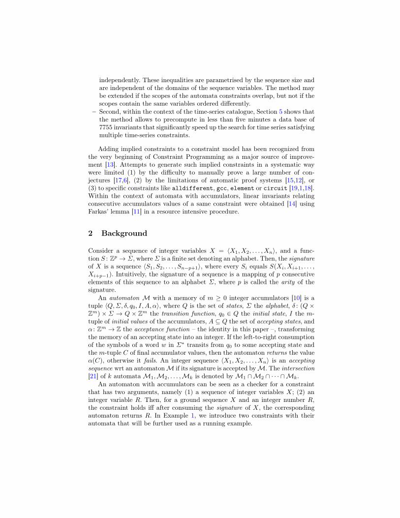
Proof. Since, when doing the intersection of automata we do not merge accu-mulators, the accumulators of I that come from different automataMi andMj

do not interact, hence the returned values ofMi andMj are independent. By

definition of the invariant digraph, the weight of any of its arc is e0 +k∑

i=1

ei · βti ,

where βti depends on the sign of ei, and where t is the corresponding transition

in I. Then, the weight ofX in GvI is the constant e+e0·(p−1)+

k∑i=1

ei·β0i (see Def-

inition 2) plus the weight of the walk of X, which is in total e+e0 ·(p−1)+k∑

i=1

ei ·

β0i +e0 ·(n−p+1)+

n−p+1∑j=1

k∑i=1

ei ·βtji = e+e0 ·n+

k∑i=1

ei ·

(β0i +

n−p+1∑j=1

βtji

), where

p is the arity of the considered signature, and t1, t2, . . . tn−p+1 is the sequence oftransitions of I triggered upon consuming the signature of X. We now show that

the value ei ·

(β0i +

n−p+1∑j=1

βtji

)is not greater than ei · Vi. This will imply that

the weight of the walk of X in GvI is less than or equal to v = e+e0 ·n+

k∑i=1

ei ·Vi.

Consider the vi = ei ·Vi linear function. We show that the weight of X in Gvi

I ,

which equals ei ·

(β0i +

n−p+1∑j=1

βtji

), is less than or equal to ei ·Vi. Depending on

the sign of ei we consider two cases.Case 1: ei ≥ 0. In this case, the weight of every arc of Gvi

I is ei multipliedby αt

ri,0, where t is the corresponding transition in I, and ri is the main accu-mulator of Mi (see Case 1 of Definition 1). If, on transition t, some potentialaccumulators of Mi are incremented by a positive constant, the real contribu-tion of the accumulator updates on this transition to Vi is at least αt

ri,0 sinceei ≥ 0. The same reasoning applies to the contribution of the initial valuesof the potential accumulators to the final value Vi. Since this contribution isnon-negative, it is ignored, and β0

i = α0ri (see Case 1 of Definition 2). Hence,

ei · (β0i +

n−p+1∑j=1

βtji ) = ei · (α0

ri +n−p+1∑j=1

αtri,0) ≤ ei · Vi.

Case 2: ei < 0. In this case, the weight of every arc of GviI is ei multiplied

by the sum of the non-negative constants, which come from the updates ofevery accumulator of Mi (see Case 2 of Definition 1). The contribution of thepotential accumulators is always taken into account, and since ei < 0, it is alwaysnegative. The same reasoning applies to the contribution of the initial values ofthe potential accumulators to the returned value Vi. Since the initial values of thepotential accumulators are non-negative, and ei < 0, in order to obtain a lowerbound on v we assume that the initial values of the potential accumulators always

contribute to Vi (see Case 2 of Definition 2). Hence, ei · (β0i +

n−p+1∑j=1

βtji ) ≤ ei ·Vi.

ut

Note that if all the considered automata M1,M2, . . . ,Mk do not have po-tential accumulators, then for every accepting sequence X = 〈X1, X2, . . . , Xn〉

wrt I =M1∩M2∩· · ·∩Mk and for any linear function v = e+e0 ·n+k∑

i=1

ei ·Vi,

the weight of X in GvI is equal to v. If there is at least one potential accumulator

for at least one automatonMi, then there may exist an integer sequence whoseweight in Gv

I is strictly less than v.

3.2 Finding the Relative Coefficients of the Linear Invariant

We now focus on finding the relative coefficients e0, e1, . . . , ek of the linear in-

variant v = e+ e0 ·n+k∑

i=1

ei ·Vi ≥ 0 such that, after consuming the signature of

any accepting sequence by the automaton I =M1 ∩M2 ∩ · · · ∩Mk, the valueof v is non-negative.

For any accepting sequenceX wrt I, by Theorem 1, we have that the weight wof X in Gv

I is less than or equal to v. Recall that w consists of a constant part,and of a part that depends on X, which involves the coefficients e0, e1, . . . , ek;thus, these coefficients must be chosen in a way that there exists a constant Csuch that w ≥ C, and C does not depend on X. This is only possible when Gv

Idoes not contain any negative cycles. Let C denote the set of all simple circuits ofGvI , and let we denote the weight of an arc e of Gv

I . In order to prevent negativecycles in Gv

I , we solve the following minimisation problem, parameterised by(s0, s1, . . . sk), the signs of e0, e1, . . . , ek:

minimise∑c∈C

Wc +

k∑i=1

|ei| (3)

subject to Wc =∑e∈c

we ∀c ∈ C (4)

Wc ≥ 0 ∀c ∈ C (5)si = ‘−’⇒ ei ≤ 0, si = ‘+’⇒ ei ≥ 0 ∀i ∈ [0, k] (6)ei 6= 0 ∀i ∈ [1, k] (7)

In order to obtain the coefficients e0, e1, . . . , ek so that GvI does not contain

any negative cycles, it is enough to find a solution to the satisfaction problem(4)-(7). Minimisation is required to obtaining invariants that eliminate as manyinfeasible values of (V1, V2, . . . , Vk) as possible. Within the objective function (3),the term

∑c∈C

Wc is for minimising the weight of every simple circuit, while the

termk∑

i=1

|ei| is for obtaining the coefficients with the smallest absolute value. By

changing the sign vector (s0, s1, . . . sk) we obtain different invariants.

Example 3. Consider peak(〈X1, X2, . . . , Xn〉 , P ) and valley(〈X1, X2, . . . , Xn〉 ,V ) from Example 2. The invariant digraph of the intersection of the automatafor the Peak and Valley constraints wrt v = e + e0 · n + e1 · P + e2 · V wasgiven in Example 2. This digraph has four simple circuits, namely s − s, t − t,

r − r, and r − t− r, which are labeled by 1, 2, 3 and 4, respectively. Then, theminimisation problem for finding the relative coefficients of the invariant v ≥ 0,parameterised by (s0, s1, s2), the signs of e0, e1 and e2, is the following:

minimise4∑

j=1

Wj+

2∑i=0

|ei|

subject to Wj =e0, ∀j ∈ [1, 3]

W4 =e0 + e1 + e2

Wj ≥ 0 ∀j ∈ [1, 4] (8)si = ‘−’⇒ ei ≤ 0, si = ‘+’⇒ ei ≥ 0 ∀i ∈ [0, 2]

ei 6= 0 ∀i ∈ [1, 2]

Note that the value of e0 must be non-negative otherwise (8) cannot besatisfied for j ∈ {1, 2, 3}. Hence, we consider only the combinations of signsof the form (‘+’, s1, s2) with s1 ans s2 being either ‘−’ or ‘+’. The followingtable gives the optimal solution of the minimisation problem for the consideredcombinations of signs:

(s0, s1, s2) (+,−,−) (+,−,+) (+,+,−) (+,+,+)(e0, e1, e2) (1,−1,−1) (0,−1, 1) (0, 1,−1) (0, 1, 1)

4

3.3 Finding the Constant Term of the Linear Invariant

Finally, we focus on finding the constant term e of the linear invariant v =

e + e0 · n +k∑

i=1

ei · Vi ≥ 0, when the coefficients e0, e1, . . . , ek are known, and

when the digraph of the automaton I =M1 ∩M2 ∩ · · · ∩Mk wrt v does notcontain any negative cycles. By Theorem 1, the weight of any accepting sequenceX wrt I in Gv

I is smaller or equal to v, then if the weight of X is non-negative,it implies that v is also non-negative. Since the digraph Gv

I does not contain anynegative cycles, then the weight of X cannot be smaller than some constant C.Hence, it suffices to find this constant and set the constant term e to −C. The

value of C is computed as the constant e0 · (p − 1) −k∑

i=1

β0i (see Definition 2)

plus the shortest path length from the node of GvI corresponding to the initial

state of I to all the nodes of GvI corresponding to the accepting states of I.

Example 4. Consider peak(〈X1, X2, . . . , Xn〉 , P ) and valley(〈X1, X2, . . . , Xn〉 ,V ) from Example 2 with n ≥ 2, i.e. the signature of 〈X1, X2, . . . , Xn〉 is notempty. In Example 3, we found four vectors for the relative coefficients e0, e1,e2 of the invariant e + e0 · n + e1 · P + e2 · V ≥ 0. For every found vector forthe relative coefficients (e0, e1, e2), we obtain a weighted digraph, whose weightsnow are integer numbers. For example, for the vector (e0, e1, e2) = (0,−1, 1),the obtained digraph is given in Part (A) of Fig. 2. We compute the length of

s

t r

0

00

00

1

−1

(A)0 1 2 3 5 6

0

1

2

4

5

6

4

3

peak

valle

y

Size: 11

P≤V+1

V≤P+1

V+P≤9

V+P≥0

(B)

110

2

< > < > < > < > = =

¬ ­ ® ¯

4 peaks︷ ︸︸ ︷

< > < > < > < > = =

¬ ­ ®︸ ︷︷ ︸3 valleys

example of sequence correspon-ding to the feasible value (4,3):0,2,0,2,0,2,0,2,0,0,0

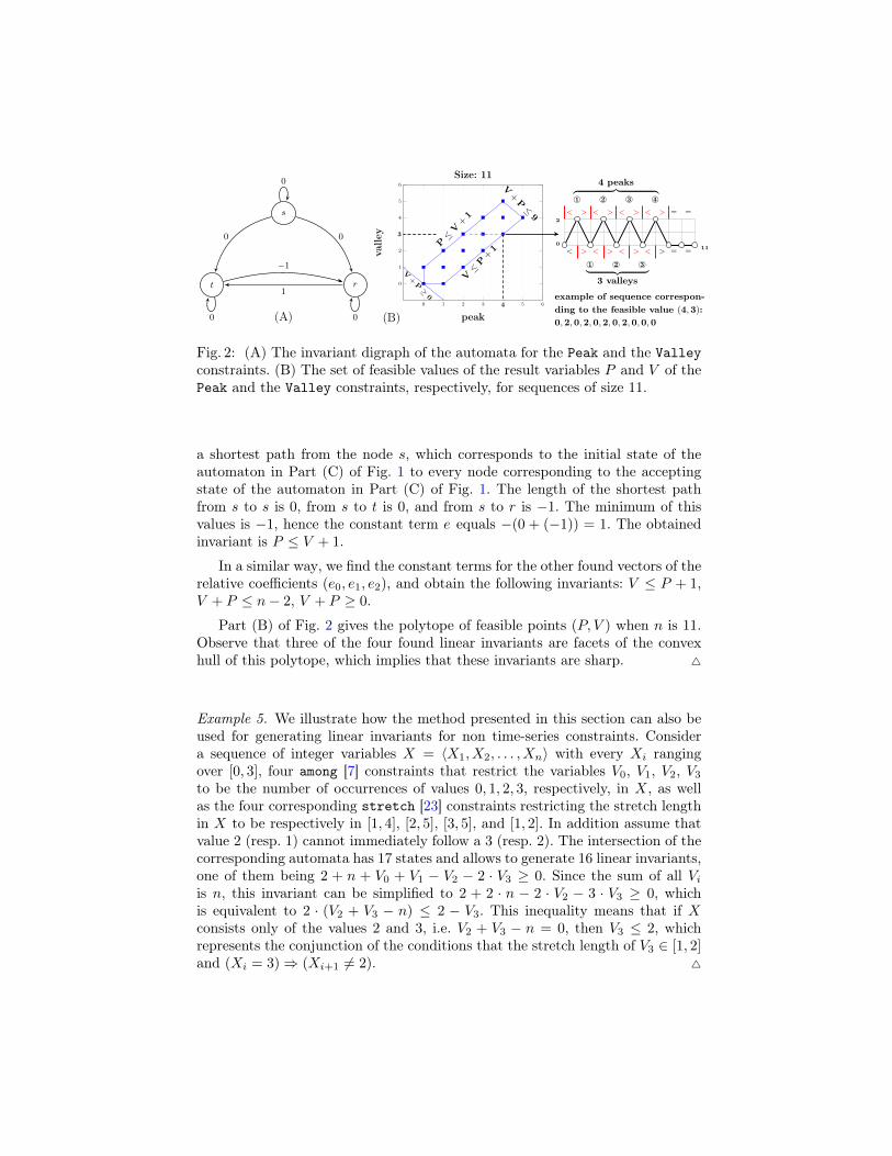
Fig. 2: (A) The invariant digraph of the automata for the Peak and the Valleyconstraints. (B) The set of feasible values of the result variables P and V of thePeak and the Valley constraints, respectively, for sequences of size 11.

a shortest path from the node s, which corresponds to the initial state of theautomaton in Part (C) of Fig. 1 to every node corresponding to the acceptingstate of the automaton in Part (C) of Fig. 1. The length of the shortest pathfrom s to s is 0, from s to t is 0, and from s to r is −1. The minimum of thisvalues is −1, hence the constant term e equals −(0 + (−1)) = 1. The obtainedinvariant is P ≤ V + 1.

In a similar way, we find the constant terms for the other found vectors of therelative coefficients (e0, e1, e2), and obtain the following invariants: V ≤ P + 1,V + P ≤ n− 2, V + P ≥ 0.

Part (B) of Fig. 2 gives the polytope of feasible points (P, V ) when n is 11.Observe that three of the four found linear invariants are facets of the convexhull of this polytope, which implies that these invariants are sharp. 4

Example 5. We illustrate how the method presented in this section can also beused for generating linear invariants for non time-series constraints. Considera sequence of integer variables X = 〈X1, X2, . . . , Xn〉 with every Xi rangingover [0, 3], four among [7] constraints that restrict the variables V0, V1, V2, V3to be the number of occurrences of values 0, 1, 2, 3, respectively, in X, as wellas the four corresponding stretch [23] constraints restricting the stretch lengthin X to be respectively in [1, 4], [2, 5], [3, 5], and [1, 2]. In addition assume thatvalue 2 (resp. 1) cannot immediately follow a 3 (resp. 2). The intersection of thecorresponding automata has 17 states and allows to generate 16 linear invariants,one of them being 2 + n + V0 + V1 − V2 − 2 · V3 ≥ 0. Since the sum of all Viis n, this invariant can be simplified to 2 + 2 · n − 2 · V2 − 3 · V3 ≥ 0, whichis equivalent to 2 · (V2 + V3 − n) ≤ 2 − V3. This inequality means that if Xconsists only of the values 2 and 3, i.e. V2 + V3 − n = 0, then V3 ≤ 2, whichrepresents the conjunction of the conditions that the stretch length of V3 ∈ [1, 2]and (Xi = 3)⇒ (Xi+1 6= 2). 4

4 Conditional Linear Invariants

In Section 3, we presented a method for generating linear invariants linking thevalues returned by an automaton I = M1 ∩M2 ∩ · · · ∩ Mk after consumingthe signature of a same accepting sequence X = 〈X1, X2, . . . , Xn〉 wrt I. Inthis section, we present several cases where the same method can be used forgenerating conditional linear invariants.

Quite often an automatonMi (with i in [1, k]) returns its initial value onlywhen the signature of X does not contain any occurrence of some regular expres-sion σi. This may lead to a convex hull of points of coordinates (V1, V2, . . . , Vk)returned by I containing infeasible points, e.g. see Part (A) of Fig. 3. Someof these infeasible points can be eliminated by stronger invariants subject tothe condition, called the non-default value condition, that no variable of the re-turned vector is assigned to the initial value of the corresponding accumulator.Section 4.1 shows to generate such invariants. Section 4.2 introduces the notion of

guard of a transition t of I, a linear inequality of the form e+e0 ·n+k∑

i=1

ei ·Vi ≥ 0,

which is a necessary condition on the vector of values returned by I after con-suming X for triggering the transition t upon consuming X.

4.1 Linear Invariants with the Non-Default Value Condition

We first illustrate the motivation for such invariants.

Example 6. Consider the nb_decreasing_terrace(〈X1, X2, . . . , Xn〉 , V1) andthe sum_width_increasing_terrace(〈X1, X2, . . . , Xn〉 , V2) constraints, whereV1 is restricted to be the number of maximal occurrences of DecreasingTerrace =‘ >=+> ’ in the signature of X = 〈X1, X2, . . . , Xn〉, and V2 is restricted to bethe sum of the number of elements in subseries of X whose signatures corre-spond to words of the language of IncreasingTerrace = ‘ <=+< ’. In Fig. 3,for n = 12, the squared points represent feasible pairs (V1, V2), while the circledpoints stand for infeasible pairs (V1, V2) inside the convex hull. The linear in-variant 2 · V1 + V2 ≤ n − 2 is a facet of the polytope, which does not eliminatethe points (1, 8), (2, 6), (3, 4), (4, 2). However, if we assume that both V1 > 0and V2 > 0, then we can add a linear invariant eliminating these four infeasiblepoints, namely 2 ·V1+V2 ≤ n−3, shown in Part (B) of Fig. 3. In addition, if weassume that V1 > 0 and V2 > 0, the infeasible points on the straight line V2 = 1will also be eliminated by the restriction V2 = 0∨V2 ≥ 2 given in [3, p. 2598]. 4

Consider that each automaton Mi (with i in [1, k]) returns its initial valueafter consuming the signature of an accepting sequence X wrt Mi iff the sig-nature of X does not contain any occurrence of some regular expression σi overthe alphabet Σ. LetM′i denote the automaton which accepts the words of thelanguage Σ∗σiΣ∗, where Σ∗ denotes any word over Σ. Then, using the methodof Section 3 we generate the invariants forM′1∩M′2∩· · ·∩M′k. These invariantshold when the non-default value condition is satisfied.

0 1 2 3 4 5

0

1

2

3

4

5

6

7

8

9

10

nb_decreasing_terrace

sum

_w

idth

_in

crea

sing

_te

rrac

e Size: 12

feasibleinfeasible

2 · V1 +

V2 ≤

12−2

(A)0 1 2 3 4 5

0

1

2

3

4

5

6

7

8

9

10

nb_decreasing_terrace

sum

_w

idth

_in

crea

sing

_te

rrac

e Size: 12

feasible2 · V1 +

V2 ≤

12−3

V2 ≥ 2

(B)

s

{P←0

V←0

}

t r

return P,V

Xi=Xi+1

Xi>Xi+1V≥P

Xi<Xi+1

P≥V

Xi=Xi+1

Xi>Xi+1Xi<Xi+1

Xi=Xi+1

Xi<Xi+1

{V←V +1}

Xi>Xi+1

{P←P+1}

(C)

Fig. 3: Invariants on the result values V1 and V2 of nb_decreasing_terraceand sum_width_increasing_terrace for a sequence size of 12 (A) with thegeneral invariants, and (B) with the Non-Default Value condition. (C) Intersec-tion automaton for Peak and Valley with the guards P ≥ V and V ≥ P ontransitions s→ t and s→ r (as for the return statement, the P and V accumu-lators in the guards refer to the final values of the corresponding accumulators).

4.2 Generating Guards for Transitions of the Intersection of SeveralAutomata

Consider k automata M1,M2, . . . ,Mk and let Vi (with i ∈ [1, k]) designatethe value returned byMi. We focus on generating necessary conditions, calledguards, introduced in Definition 3, for enabling transitions of the automatonI =M1∩M2∩· · ·∩Mk. Further, we give a three-step procedure for generatingguards for transitions of I.

Definition 3. Consider a transition t of the automaton I =M1∩M2∩· · ·∩Mk.

A guard of t is a linear inequality of the form e+ e0 ·n+k∑

i=1

ei ·Vi ≥ 0 such that

there does not exist any accepting sequence X = 〈X1, X2, . . . , Xn〉 wrt I suchthat (1) after consuming the signature of X, the vector (V1, V2, . . . , Vk) returned

by I satisfies the inequality e + e0 · n +k∑

i=1

ei · Vi < 0, (2) and the transition t

was triggered upon consuming the signature of X.

The following example illustrates Definition 3.

Example 7. Given a sequence X = 〈X1, X2, . . . , Xn〉, consider the peak(X,P )and valley(X,V ) constraints. The intersection I of the automata for peak andvalley was given in Part (C) of Fig. 1. Observe that, if at the initial state s theautomaton consumes ‘<’ (resp. ‘>’), then the number of peaks (resp. valleys) inX is greater than or equal to the number of valleys (resp. peaks). Hence, we canimpose the guard P ≥ V (resp. V ≥ P ) on the transition from s to t (resp. tor). Part (C) of Fig. 3 gives the automaton I with the obtained guards. 4

Guards for the transitions of an automaton I =M1 ∩M2 ∩ · · · ∩Mk canbe generated in three steps:

1. First, we identify the subset T of transitions of I such that, for any transitiont in T , upon consuming any sequence, t can be triggered at most once.

2. Second, for every transition t in T , we obtain a new automaton It by re-moving from I all transitions of T different from t that start at the samestate as t.

3. Third, using the technique of Section 3 on the invariant digraph GvIt , we

obtain linear invariants that are guards of transition t.

5 Evaluation

To test the effectiveness of the generated invariants, we first try systematic testson the conjunction of pairs of the 35 time-series constraints [5] of the nb andsum_width families for which the glue matrix constraints exist [2]. The nb con-straints count the number of occurrences of some pattern in a time series, whilethe sum_width family constrains the sum of the width of pattern occurrences.Our intended use case is similar to [9], where constraints and parameter ranges ofthe problem are learned from real-world data, and are used to produce solutionsthat are similar to the previously observed data. It is important both to removeinfeasible parameter combinations quickly, as well as helping to find solutionsfor feasible problems. Real world datasets often will only show a tiny subset ofall possible parameter combinations, but as we don’t know the data a priori, asystematic evaluation seems the most conservative approach.

For the experiments we use a database of generated invariants in a formatcompatible with the Global Constraint Catalogue [3]. Invariants are generatedas Prolog facts, from which executable code, and other formats are then pro-duced automatically. The time required to produce the invariants (5 min) isinsignificant compared to the overall runtime of the experiments. For the 595combinations of the 35 constraints we produce over 4100 unconditional invari-ants, over 3500 conditional invariants, and 86 guard invariants. In the test, wetry each pair of constraints and try to find solutions for all possible pairs ofparameter values. We compare four different versions of our methods: The purebaseline version uses the automata that were described in [4], the bounds on theparameter values for each prefix and suffix, and the glue matrix constraints asdescribed in [2]. This version represents the state of the art before the currentwork. In the invariant version we add the generated invariants for the param-eters of the complete time series. In the incremental version, we not only statethe invariants for the complete time series, but also apply them for each suffix.The required variables are already available as part of the glue matrix setup,we only need to add the linear inequalities for each suffix length. In the all ver-sion, we add the product automaton of the conjunction of the two constraints, ifit contains guard constraints, and also state some additional, manually derivedinvariants.

The test program uses a labeling routine that first assigns the signaturevariables, and only afterwards assigns values for the Xi decision variables. Thevariables in each case are assigned from left to right. For each pair of parameters

values, defined by the product of the bounds from [2], we try to find a firstsolution with a timeout of 60s.

Fig. 4: Comparing Constraint Variants,Undecided Instances Percentage for Size18 as a Function of Time, Timeout=60s

0.01

0.1

1

10

100

10 100 1000 10000 100000

Perc

enta

ge o

f In

stan

ces

Und

ecid

ed

Time [ms]

Time Needed, Size 18, Total Instances 109682

pureinv

incrall

We have tested the results for dif-ferent time series length, Figure 4shows the result for length 18 and do-main size 0..18, the largest problemsize where we find solutions for eachcase within the timeout. All experi-ments were run on a laptop with Inteli7 CPU (2.9GHz), 64Gb main mem-ory and Windows 10 64bit OS usingSICStus Prolog 4.3.5 utilizing a sin-gle core. For our four problem vari-ants, we plot the percentage of unde-cided problem instances as a functionof computation time. The plot useslog-log scales to more clearly show the values for short runtimes and for lownumber of undecided problems. The baseline pure variant solves around 55% ofthe instances immediately, and leaves just under one percent unsolved withinthe timeout. The invariants version improves on this by pruning more infeasi-ble problems immediately. On the other hand, stating the invariants on the fullseries has no effect on feasible instances. When using the incremental versionof the constraints, this has very little additional impact on infeasible problems,but improves the solution time for the feasible instances significantly. Adding(variant all) additional constraints further reduces the number of backtracksrequired, but these savings are largely balanced with the additional processingtime, and therefore have no major impact on the overall results. After one sec-ond, around 9.5% of all instances are unsolved in the baseline, but only 0.5% inthe incremental or all variant.

To test the method in a more realistic setting, we consider the conjunctionof all 35 considered time-series constraints on electricity demand data providedby an industrial partner. The time-series describes daily demand levels in half-hour intervals, giving 48 data points. To capture the shape of the time-seriesmore accurately, we split the series into overlapping segments from 00-12, 06-18, and 12-24 hours, each segment containing 24 data points, overlapping in12 data points with the previous segment. We then setup the conjunction ofthe 35 time-series constraints for each segment, using the pure and incrementalvariants described above. This leads to 3 × 35 × 2 = 210 automata constraintswith shared signature and decision variables. The invariants are created for everypair of constraints, and every suffix, leading to a large number of inequalities.The search routine assigns all signature variables from left to right, and thenassigns the decision variables, with a timeout of 120s.

In order to understand the scalability of the method, we also consider timeseries of 44 resp. 50 data points (three segments of length 22 and 25), extractedfrom the daily data stream covering a four year period (1448 samples). In Fig-

Fig. 5: Percentage of Problems Solved for 3 Overlapping Segments of Lengths22, 24, and 25; Execution time in top row, backtracks required in bottom row

0

10

20

30

40

50

60

70

80

90

100

0 20000 40000 60000 80000 100000 120000 140000

Perc

enta

ge o

f In

stan

ces

Solv

ed

Time [ms]

3 Segments, Width 22

pureincremental

(a) Time, Size 22

0

10

20

30

40

50

60

70

80

90

100

0 20000 40000 60000 80000 100000 120000 140000

Perc

enta

ge o

f In

stan

ces

Solv

ed

Time [ms]

3 Segments, Width 24

pureincremental

(b) Time, Size 24

0

10

20

30

40

50

60

70

80

90

0 20000 40000 60000 80000 100000 120000 140000

Perc

enta

ge o

f In

stan

ces

Solv

ed

Time [ms]

3 Segments, Width 25

pureincremental

(c) Time, Size 25

0

10

20

30

40

50

60

70

80

90

100

0 5000 10000 15000 20000 25000

Perc

enta

ge o

f In

stan

ces

Solv

ed

Backtracks

3 Segments, Width 22

pureincremental

(d) Backtracks, Size 22

0

10

20

30

40

50

60

70

80

90

100

0 2000 4000 6000 8000 10000 12000 14000 16000 18000 20000

Perc

enta

ge o

f In

stan

ces

Solv

ed

Backtracks

3 Segments, Width 24

pureincremental

(e) Backtracks, Size 24

0

10

20

30

40

50

60

70

80

90

0 5000 10000 15000 20000 25000 30000

Perc

enta

ge o

f In

stan

ces

Solv

ed

Backtracks

3 Segments, Width 25

pureincremental

(f) Backtracks, Size 25

ure 5 we show the time and backtrack profiles for finding a first solution. Thetop row shows the percentage of instances solved within a given time budget, thebottom row shows the percentage of problems solved within a backtrack budget.For easy problems, the pure variant finds solutions more quickly, but the incre-mental version pays off for more complex problems, as it reduces the number ofbacktracks required sufficiently to account for the large overhead of stating andpruning all invariants. The problems for segment length 20 (not shown) can besolved without timeout for both variants, as the segment length increases, thenumber of time outs increases much more rapidly for the pure variant. Addingthe invariants drastically reduces the search space in all cases, future work shouldconsider if we can identify those invariants that actively contribute to the searchby cutting off infeasible branches early on. Restricting the invariants to such anactive subset should lead to a further improvement in execution time.

6 Conclusion

Future work may look how to extend the current approach to handle automatawith accumulators that also allow the min and max aggregators for accumulatorupdates. It also should investigate the use of such invariants within the contextof MIP. While MIP has been using linear cuts for a long time [16,20], no off-the-shelf data base of cuts in some computer readable format is currently available.Cuts are typically defined in papers and are then directly embedded within MIPsolvers.

References

1. Appa, G., Magos, D., Mourtos, I.: LP relaxations of multiple all_different pred-icates. In: Régin, J.C., Rueher, M. (eds.) Integration of AI and OR Techniques inConstraint Programming for Combinatorial Optimization Problems, First Interna-tional Conference, CPAIOR 2004. LNCS, vol. 3011, pp. 364–369. Springer (2004)

2. Arafailova, E., Beldiceanu, N., Carlsson, M., Flener, P., Francisco Rodríguez, M.A.,Pearson, J., Simonis, H.: Systematic derivation of bounds and glue constraints fortime-series constraints. In: Rueher, M. (ed.) CP 2016. LNCS, vol. 9892, pp. 13–29.Springer (2016)

3. Arafailova, E., Beldiceanu, N., Douence, R., Carlsson, M., Flener, P., Rodríguez,M.A.F., Pearson, J., Simonis, H.: Global constraint catalog, volume ii, time-seriesconstraints. CoRR abs/1609.08925 (2016), http://arxiv.org/abs/1609.08925

4. Arafailova, E., Beldiceanu, N., Douence, R., Flener, P., Francisco Rodríguez, M.A.,Pearson, J., Simonis, H.: Time-series constraints: Improvements and application inCP and MIP contexts. In: Quimper, C.G. (ed.) CP-AI-OR 2016. LNCS, vol. 9676,pp. 18–34. Springer (2016)

5. Beldiceanu, N., Carlsson, M., Douence, R., Simonis, H.: Using finite transduc-ers for describing and synthesising structural time-series constraints. Constraints21(1), 22–40 (January 2016), journal fast track of CP 2015: summary on p. 723 ofLNCS 9255, Springer, 2015

6. Beldiceanu, N., Carlsson, M., Rampon, J.X., Truchet, C.: Graph invariants asnecessary conditions for global constraints. In: van Beek, P. (ed.) Principles andPractice of Constraint Programming - CP 2005, 11th International Conference, CP2005. LNCS, vol. 3709, pp. 92–106. Springer (2005)

7. Beldiceanu, N., Contejean, E.: Introducing global constraints in CHIP. Mathl.Comput. Modelling 20(12), 97–123 (1994)

8. Beldiceanu, N., Flener, P., Pearson, J., Van Hentenryck, P.: Propagating regularcounting constraints. In: Brodley, C.E., Stone, P. (eds.) AAAI 2014. pp. 2616–2622.AAAI Press (2014)

9. Beldiceanu, N., Ifrim, G., Lenoir, A., Simonis, H.: Describing and generating so-lutions for the EDF unit commitment problem with the ModelSeeker. In: Schulte,C. (ed.) CP 2013. LNCS, vol. 8124, pp. 733–748. Springer (2013)

10. Beldiceanu, N., Mats, C., Petit, T.: Deriving filtering algorithms from constraintcheckers. In: Wallace, M. (ed.) Principles and Practice of Constraint Programming- CP 2004, 10th International Conference, CP 2004. LNCS, vol. 3258, pp. 107–122.Springer (2004)

11. Boyd, S.P., Vandenberghe, L.: Convex Optimization. Cambridge University Press(2004)

12. Charnley, J.W., Colton, S., Miguel, I.: Automatic generation of implied constraints.In: ECAI 2006. Frontiers in AI and Applications, vol. 141, pp. 73–77. IOS Press(2006)

13. Dincbas, M., Simonis, H., Hentenryck, P.V.: Solving the car-sequencing problemin constraint logic programming. In: ECAI. pp. 290–295 (1988)

14. Francisco Rodríguez, M.A., Flener, P., Pearson, J.: Implied constraints for Au-tomaton constraints. In: Gottlob, G., Sutcliffe, G., Voronkov, A. (eds.) GCAI 2015.EasyChair Proceedings in Computing, vol. 36, pp. 113–126 (2015)

15. Frisch, A., Miguel, I., Walsh, T.: Extensions to proof planning for generating im-plied constraints. In: 9th Symp. on the Integration of Symbolic Computation andMechanized Reasoning (2001)

16. Gomory, R.: Outline of an algorithm for integer solutions to linear programs. Bul-letin of the American Mathematical Society 64, 275–278 (1958)

17. Hansen, P., Caporossi, G.: Autographix: An automated system for finding conjec-tures in graph theory. Electronic Notes in Discrete Mathematics 5, 158–161 (2000)

18. Hooker, J.N.: Integrated Methods for Optimization. Springer Publishing Company,Incorporated, 2nd edn. (2011)

19. Lee, J.: All-different polytopes. J. Comb. Optim. 6(3), 335–352 (2002)20. Marchand, H., Martin, A., Weismantel, R., Wolsey, L.A.: Cutting planes in integer

and mixed integer programming. Discrete Applied Mathematics 123(1-3), 397–446(2002)

21. Menana, J.: Automata and Constraint Programming for Personnel Schedul-ing Problems. Theses, Université de Nantes (Oct 2011), https://tel.archives-ouvertes.fr/tel-00785838

22. Menana, J., Demassey, S.: Sequencing and counting with the multicost-regularconstraint. In: Integration of AI and OR Techniques in Constraint Programmingfor Combinatorial Optimization Problems, 6th International Conference, CPAIOR2009, Pittsburgh, PA, USA, May 27-31, 2009, Proceedings. pp. 178–192 (2009)

23. Pesant, G.: A filtering algorithm for the stretch constraint. In: Walsh, T. (ed.)CP 2001. LNCS, vol. 2239, pp. 183–195. Springer (2001)