Embed Size (px)
Citation preview
General Summary of Recommended Travel Demand
Model Development Procedures for
Consultants, MPOs and Modelers
Prepared for
GDOT
May 2013

This document is subject to change without notice. Please verify with GDOT staff to confirm
that this is the most current version.
i
TableofContents
1 Introduction ............................................................................................................................. 1
2 Highway Network .................................................................................................................. 1
2.1 Levels of Links (Screenlines, Cutlines and Cordon Lines) ...................................................... 6
2.2 Additional Variables ..................................................................................................................... 8 2.2.1 Turn Prohibitors ................................................................................................................................... 11 2.2.2 Identifying Facilities for Network Coding ........................................................................................ 12
3 Defining Traffic Analysis Zones ....................................................................................... 13
3.1 Creating Traffic Analysis Zones ................................................................................................ 13 3.1.1 How to Select Appropriate TAZ Boundaries ................................................................................... 13 3.1.2 Use of Census Information ................................................................................................................. 14 3.1.3 Major Topographic Barriers ................................................................................................................ 17 3.1.4 Modeled Highway Network ............................................................................................................... 18 3.1.5 Zonal Homogeneity ............................................................................................................................. 18 3.1.6 Other General Guidelines ................................................................................................................... 19 3.1.7 Estimated Number of Zones ............................................................................................................... 19 3.1.8 Procedure for Numbering ................................................................................................................... 20
4 Socio-Economic Data ............................................................................................................ 21
4.1 Base Year Data .............................................................................................................................. 23 4.1.1 Population, Households, and Income ............................................................................................... 23 4.1.2 Employment by Type .......................................................................................................................... 24 4.1.3 School Enrollment ................................................................................................................................ 27 4.1.4 Acres ...................................................................................................................................................... 27
4.2 Future Year Projections ............................................................................................................... 27 4.2.1 Population and Households ............................................................................................................... 28 4.2.2 Median Income ..................................................................................................................................... 29 4.2.3 Employment by Type .......................................................................................................................... 29 4.2.4 School Enrollment ................................................................................................................................ 30 4.2.5 Acres ...................................................................................................................................................... 30
4.3 Procedures to Check the Data .................................................................................................... 30 4.3.1 Population per Household Ratio........................................................................................................ 30 4.3.2 Households (Occupied) ....................................................................................................................... 31 4.3.3 Households per Acre ........................................................................................................................... 31 4.3.4 Employment .......................................................................................................................................... 31 4.3.5 Workforce Utilization .......................................................................................................................... 31 4.3.6 Income.................................................................................................................................................... 31 4.3.7 School Enrollment ................................................................................................................................ 31
5 External Model Development............................................................................................. 32
6 Trip Generation ..................................................................................................................... 32
6.1 Traffic Analysis Zone Data ......................................................................................................... 33
ii
6.2 Production Model ........................................................................................................................ 33 6.2.1.1 Household Stratification Sub-Model ......................................................................................... 36
6.3 Attraction Model .......................................................................................................................... 39
6.4 Trucks ............................................................................................................................................ 39
6.5 External Trips ............................................................................................................................... 40
6.6 Trip Generation Calibration/Validation .................................................................................. 40
6.7 Final Documentation ................................................................................................................... 41
7 Trip Distribution Calibration/Validation ........................................................................ 41
7.1 Final Documentation ................................................................................................................... 42
8 Mode Choice .......................................................................................................................... 43
9 Trip Assignment.................................................................................................................... 43
9.1 Highway Assignment Calibration/Validation........................................................................ 43 9.1.1 Poor Calibration Practices – What Not to Do ................................................................................... 44 9.1.2 Final Documentation ........................................................................................................................... 45
10 Review of MPO Model Development Activities .......................................................... 45
11 File Naming Conventions ................................................................................................. 46
12 Potential Treatment of Military Bases ............................................................................ 47
12.1 Treatment of Military Bases as Special Generators ............................................................... 47 12.1.1 Trip generation ................................................................................................................................... 47 12.1.2 Trip distribution ................................................................................................................................. 47
12.2 Treatment of Military Bases as a Separated Trip Purpose ................................................... 47 12.2.1 Trip generation ................................................................................................................................... 47 12.2.2 Trip distribution ................................................................................................................................. 48
APPENDIX ................................................................................................................................ 49
A-1: Socio-Economic Data Preparation Checklist and Review Guidelines ............................. 50
A-2: Checklist for Preparing Highway Networks ........................................................................ 53
A-3: Level of Service V/C Ratio Breakpoints ............................................................................... 55
A-4: MPO Model Daily Capacity Measure ................................................................................... 57
GLOSSARY ............................................................................................................................... 59
iii
List of Tables
Table 2-1 - Highway Network Variables ............................................................................... 2
Table 2-2 – Facility Type Descriptions ................................................................................... 3
Table 2-3 - Facility Type Characteristics ................................................................................ 5
Table 2-4 – Area Type Definitions .......................................................................................... 8
Table 2-5 – Example Area Type Lookup Table .................................................................... 9
Table 2-6 - Example Area Type Lookup (Combined Densities) ....................................... 9
Table 2-7 - Hourly Capacities per Lane ................................................................................ 10
Table 2-8 - Free-Flow Speed Matrix ...................................................................................... 11
Table 3-1 - Rules of Thumb for Estimating Number of Traffic Zones .......................... 19
Table 4-1 - Socio-Economic and General Data Required by TAZ .................................. 23
Table 4-2 - GDOT NAICS Employment Equivalency Table ........................................... 25
Table 4-3 - Potential TAZ Land Use Database Variables ................................................. 27
Table 6-1 - Default GDOT Daily Trip Production Rates ................................................. 33
Table 11-1 - Model File Naming Protocols .......................................................................... 46
List of Figures
Figure 2-1 - Example of Screenline Locations ...................................................................... 7
Figure 2-2 - Example of Cutline Locations ........................................................................... 7
Figure 2-3 - Example of Cordon Location ............................................................................. 8
Figure 3-1 - US Census Bureau Geography ......................................................................... 15
Figure 3-2 – Census TAD and TAZ boundaries ................................................................. 16
Figure 3-3 - Traffic Analysis Zone Guidelines ................................................................... 17
Figure 4-1 – Generalized Travel Model Socio-Economic Data Development Process22
Figure 11-1 – Model Folder Structure ................................................................................... 46

Summary of Recommended Travel Demand Model Development Procedures 1
1 Introduction
This document provides a general summary of the recommended key procedures to develop travel demand models for the Georgia Department of Transportation (GDOT). This document also briefly describes the format of the input data sets required for the development of a travel demand model such as socio-economic data, traffic analysis zones, and highway networks. The purpose of this document is to provide the Georgia MPOs and consultants with information about the Georgia regional travel demand models, as well as to provide assistance and direction on the preparation of socio-economic data and highway networks, which is vital to the development and application of the travel demand models. In addition, naming conventions for the model output files and a folder structure are described. If MPOs and/or their Consultants are building their own travel demand model that may be used for the development of a Long Range Transportation Plan (LRTP), GDOT requests that the MPOs/consultants follow this guide as closely as possible.
2 Highway Network
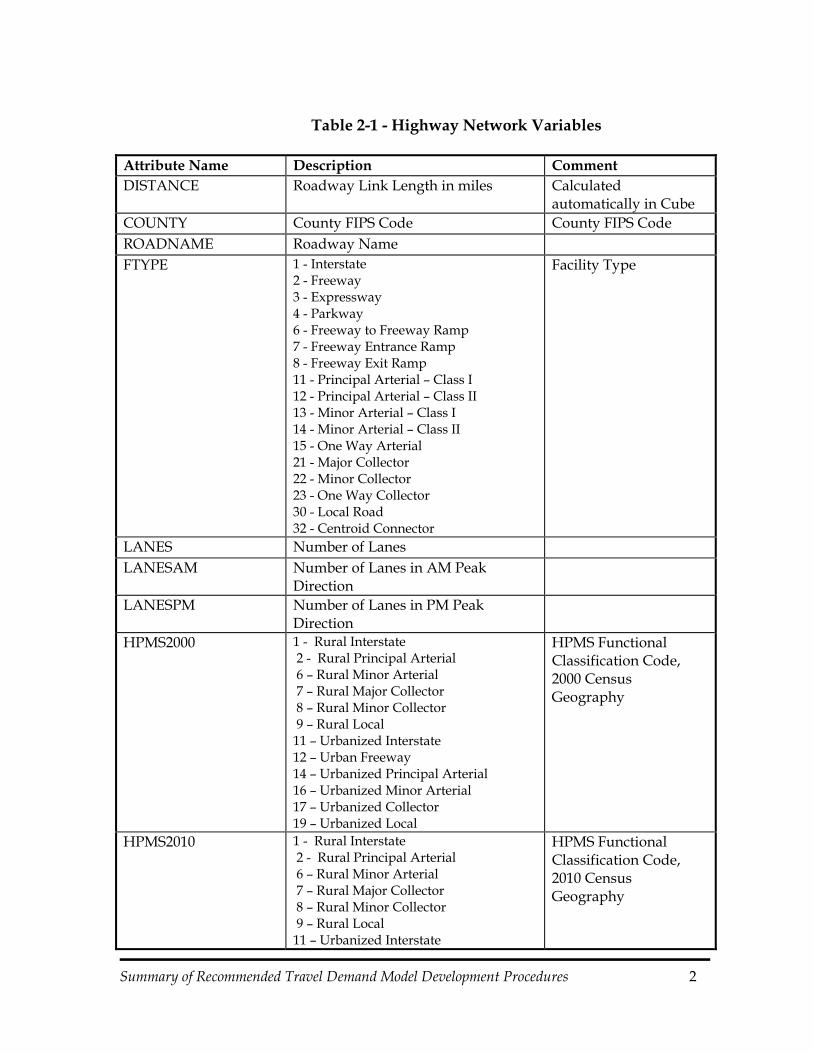
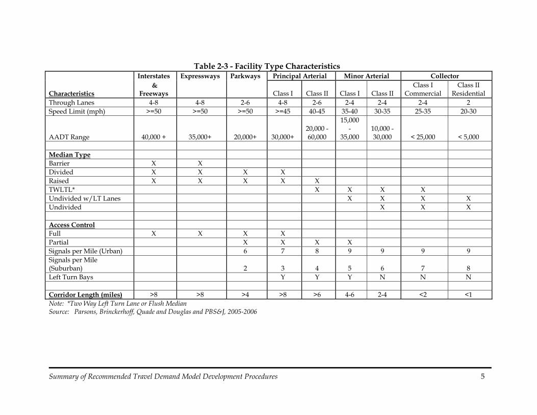
GDOT has recently established naming conventions for the attributes in the highway networks for all of the models. Table 2-1 summarizes the primary highway network link field names. There have been some variations in the field names from one MPO network to another in the past. As each model is updated, fieldname/attributes must be revised. There is a list in the Appendix that outlines a set of network checks that GDOT recommend be utilized. There are some network variables that may no longer be needed when creating a new network. These variables have been included in previous networks through the years, such as the 1990 functional classification and previous calibration year traffic counts. Table 2-2 provides general descriptions of the GDOT facility types and Table 2-3 provides common characteristics of each.
Summary of Recommended Travel Demand Model Development Procedures 2
Table 2-1 - Highway Network Variables
Attribute Name Description Comment DISTANCE Roadway Link Length in miles Calculated
automatically in Cube COUNTY County FIPS Code County FIPS Code ROADNAME Roadway Name FTYPE 1 - Interstate
2 - Freeway 3 - Expressway 4 - Parkway 6 - Freeway to Freeway Ramp 7 - Freeway Entrance Ramp 8 - Freeway Exit Ramp 11 - Principal Arterial – Class I 12 - Principal Arterial – Class II 13 - Minor Arterial – Class I 14 - Minor Arterial – Class II 15 - One Way Arterial 21 - Major Collector 22 - Minor Collector 23 - One Way Collector 30 - Local Road 32 - Centroid Connector
Facility Type
LANES Number of Lanes LANESAM Number of Lanes in AM Peak
Direction
LANESPM Number of Lanes in PM Peak Direction
HPMS2000 1 - Rural Interstate 2 - Rural Principal Arterial 6 – Rural Minor Arterial 7 – Rural Major Collector 8 – Rural Minor Collector 9 – Rural Local 11 – Urbanized Interstate 12 – Urban Freeway 14 – Urbanized Principal Arterial 16 – Urbanized Minor Arterial 17 – Urbanized Collector 19 – Urbanized Local
HPMS Functional Classification Code, 2000 Census Geography
HPMS2010 1 - Rural Interstate 2 - Rural Principal Arterial 6 – Rural Minor Arterial 7 – Rural Major Collector 8 – Rural Minor Collector 9 – Rural Local 11 – Urbanized Interstate
HPMS Functional Classification Code, 2010 Census Geography

Summary of Recommended Travel Demand Model Development Procedures 3
Attribute Name Description Comment 12 – Urban Freeway 14 – Urbanized Principal Arterial 16 – Urbanized Minor Arterial 17 – Urbanized Collector 19 – Urbanized Local
CSTATION Traffic Count Station Number Zero if not a count station
TCOUNTyear Year AADT - Two Way - Both Directions (from GDOT QA/QC Database)
Zero if not a count station
COUNTyear Year AADT - One Way (Directional) Zero if not a count station
SCREENLINE Screenline ID 0 if not on a screenline CUTLINE Cutline ID 0 if not on a cutline UAB2010 Urbanized Area Code, 2010 Census
Geography
GDOT_PI GDOT Project Identification Number
Numeric
LOCAL_PI Local Project Identification Number If no GDOT PI number is available – Numeric values are required
OPEN_DATE Model Year Open to Traffic – Construction Completed
TOLL (OPTIONAL)
Cost of toll in dollars (if applicable) Converted to time penalty during model run (not in all models)
MODEL YEAR (OPTIONAL)
Open to Construction Required for air quality analysis
AADT_#### Current Year Traffic Count– Two Way
Zero if not a count station
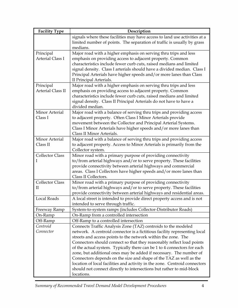
Table 2-2 – Facility Type Descriptions
Facility Type Description Interstate - Freeway
Limited Access Highway Mainline (includes Interstates) – Serves trips traveling longer distances. These facilities are not intended or designed to provide direct access to land use activities. Access is limited to interchange points.
Expressway Controlled Access Highway - Serves trips traveling longer distances but usually not as long as freeways and within an urban area. These facilities are not designed to provide direct access to land use activities. Access is managed to minimize the degradation to capacity while providing access to abutting land uses. The separation of traffic is usually by concrete barriers.
Parkway Controlled Access Highway –These facilities are usually not designed to expressway and/or interstate standards. There may be traffic
Summary of Recommended Travel Demand Model Development Procedures 4
Facility Type Description signals where these facilities may have access to land use activities at a limited number of points. The separation of traffic is usually by grass medians.
Principal Arterial Class I
Major road with a higher emphasis on serving thru trips and less emphasis on providing access to adjacent property. Common characteristics include fewer curb cuts, raised medians and limited signal density. Class I arterials should have a divided median. Class I Principal Arterials have higher speeds and/or more lanes than Class II Principal Arterials.
Principal Arterial Class II
Major road with a higher emphasis on serving thru trips and less emphasis on providing access to adjacent property. Common characteristics include fewer curb cuts, raised medians and limited signal density. Class II Principal Arterials do not have to have a divided median.
Minor Arterial Class I
Major road with a balance of serving thru trips and providing access to adjacent property. Often Class I Minor Arterials provide movement between the Collector and Principal Arterial Systems. Class I Minor Arterials have higher speeds and/or more lanes than Class II Minor Arterials.
Minor Arterial Class II
Major road with a balance of serving thru trips and providing access to adjacent property. Access to Minor Arterials is primarily from the Collector system.
Collector Class I
Minor road with a primary purpose of providing connectivity to/from arterial highways and/or to serve property. These facilities provide connectivity between arterial highways and commercial areas. Class I Collectors have higher speeds and/or more lanes than Class II Collectors.
Collector Class II
Minor road with a primary purpose of providing connectivity to/from arterial highways and/or to serve property. These facilities provide connectivity between arterial highways and residential areas.
Local Roads A local street is intended to provide direct property access and is not intended to serve through traffic.
Freeway Ramp System-to-system ramps (includes Collector-Distributor Roads) On-Ramp On-Ramp from a controlled intersection Off-Ramp Off-Ramp to a controlled intersection Centroid Connector
Connects Traffic Analysis Zone (TAZ) centroids to the modeled network. A centroid connector is a fictitious facility representing local streets and access points to the network within the zone. The Connectors should connect so that they reasonably reflect load points of the actual system. Typically there can be 1 to 4 connectors for each zone, but additional ones may be added if necessary. The number of Connectors depends on the size and shape of the TAZ as well as the location of local facilities and activity in the zone. Centroid connectors should not connect directly to intersections but rather to mid-block locations.
Summary of Recommended Travel Demand Model Development Procedures 5
Table 2-3 - Facility Type Characteristics Interstates Expressways Parkways Principal Arterial Minor Arterial Collector
Characteristics &
Freeways Class I Class II Class I Class II Class I
Commercial Class II
Residential Through Lanes 4-8 4-8 2-6 4-8 2-6 2-4 2-4 2-4 2 Speed Limit (mph) >=50 >=50 >=50 >=45 40-45 35-40 30-35 25-35 20-30
AADT Range 40,000 + 35,000+ 20,000+ 30,000+ 20,000 - 60,000
15,000 -
35,000 10,000 - 30,000 < 25,000 < 5,000
Median Type Barrier X X Divided X X X X Raised X X X X X TWLTL* X X X X Undivided w/LT Lanes X X X X Undivided X X X Access Control Full X X X X Partial X X X X Signals per Mile (Urban) 6 7 8 9 9 9 9 Signals per Mile (Suburban) 2 3 4 5 6 7 8 Left Turn Bays Y Y Y N N N Corridor Length (miles) >8 >8 >4 >8 >6 4-6 2-4 <2 <1 Note: *Two Way Left Turn Lane or Flush Median Source: Parsons, Brinckerhoff, Quade and Douglas and PBS&J, 2005-2006
Summary of Recommended Travel Demand Model Development Procedures 6
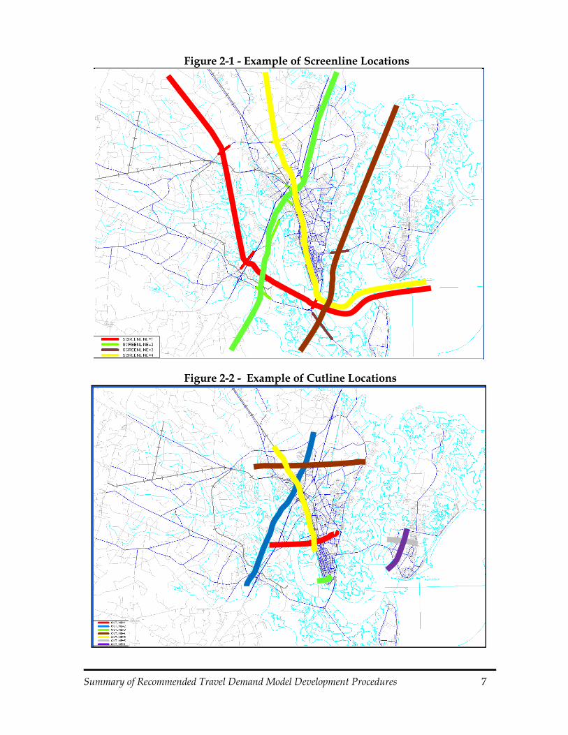
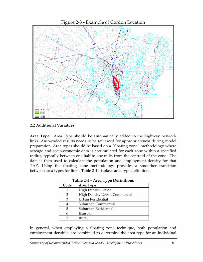
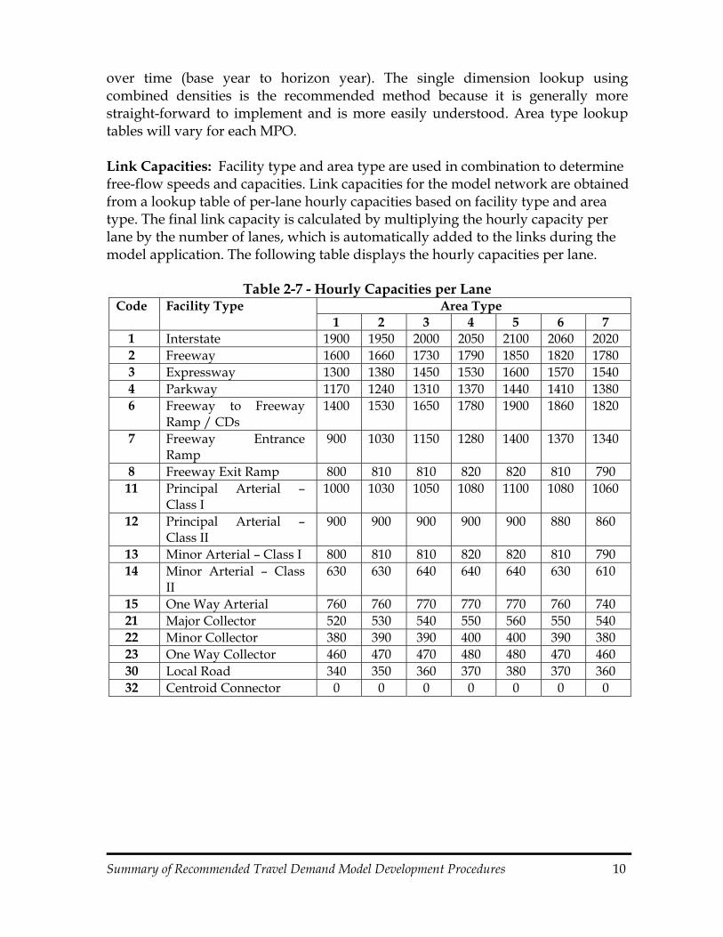
2.1 Levels of Links (Screenlines, Cutlines and Cordon Lines) Screenlines and cutlines are imaginary lines that are used to assess model validation. Comparison of modeled versus counted traffic across cordons or screenlines provides an indication of how well a travel demand model performs in replicating major trip patterns and movements throughout the network. The screenline or cordon will usually correspond with a recognized visible boundary feature (a river or major transportation facility) or a well-delineated political boundary (a county or city border). Screenlines typically encompass all facilities that serve the same definable travel corridor to allow for the fact that the model may not perfectly represent competition between parallel facilities. These are described below and shown in the Figures 2.1 through 2.3 below: Screenlines typically extend completely across the modeled area and go from boundary cordon to boundary cordon. Screenlines capture cross-regional travel flows. For example, a river that passes completely through the area makes an excellent screenline. Travel demand that goes from one side of the river to the other must cross this river screenline within the study area boundary. Screenlines are most often associated with physical barriers such as interstates, rivers or railroads and serve as Traffic Analysis Zone (TAZ) boundaries. Cutlines extend across a corridor containing multiple facilities. They should be used to intercept travel along only one axis. Screenlines usually cover “major” regional travel patterns, but as major destinations become more dispersed, the major travel patterns also become more dispersed, and at that point, cutlines may be employed to look at particular locations and corridors. Cordon lines completely encompass a designated area. Cordon lines are typically associated with the boundary of the area being modeled. However, for model validation purposes, it is also helpful to develop internal cordon lines or boundaries. For example, a cordon around the central business district is useful in validating the "ins and outs" of the CBD related traffic demand. Over or under estimates of trips bound for the CBD could indicate errors in the socioeconomic data (employment data for the CBD) or errors in the trip distribution or mode choice model. An example of screenlines for a Georgia MPO is illustrated in Figure 2-1, an example of cutlines in Figure 2-2 and an example of a cordon line in Figure 2-3.
Summary of Recommended Travel Demand Model Development Procedures 7
Figure 2-1 - Example of Screenline Locations
Figure 2-2 - Example of Cutline Locations
Summary of Recommended Travel Demand Model Development Procedures 8
Figure 2-3 - Example of Cordon Location
2.2 Additional Variables Area Type: Area Type should be automatically added to the highway network links. Auto-coded results needs to be reviewed for appropriateness during model preparation. Area types should be based on a “floating zone” methodology where acreage and socio-economic data is accumulated for each zone within a specified radius, typically between one-half to one mile, from the centroid of the zone. The data is then used to calculate the population and employment density for that TAZ. Using the floating zone methodology provides a smoother transition between area types for links. Table 2-4 displays area type definitions.
Table 2-4 – Area Type Definitions Code Area Type
1 High Density Urban 2 High Density Urban Commercial 3 Urban Residential 4 Suburban Commercial 5 Suburban Residential 6 Exurban 7 Rural
In general, when employing a floating zone technique, both population and employment densities are combined to determine the area type for an individual

Summary of Recommended Travel Demand Model Development Procedures 9
zone. GDOT models have historically employed an approach that develops separate floating zone population and employment densities, then area types are obtained from a two-dimensional lookup table. Table 2-5 shows an example two-dimensional area type lookup table. Population and employment density ranges used in the lookup table are typically selected percentiles of the calculated floating zone results. Particular percentile values are chosen by evaluating the resulting area types to determine if expected results are being produced. If not, then different percentile range values are selected, until acceptable results are produced.
Table 2-5 – Example Area Type Lookup Table
Population Density (per acre)
Employment Density (per acre)
Low High Low 0.00 0.01 0.31 2.00 6.76 9.43 25.17High 0.01 0.31 2.00 6.76 9.43 25.17 ∞
0.00 0.05 7 7 6 4 3 3 1 0.05 0.22 7 6 6 4 3 3 1 0.22 0.59 6 6 5 4 3 2 1 0.59 0.83 6 6 5 4 3 2 1 0.83 3.73 5 5 5 4 3 2 1 3.73 5.57 5 5 4 3 3 2 1 5.57 ∞ 5 5 4 3 2 2 1
Future GDOT models can use another method to combine the population and employment densities. This alternate approach combines the two density values with a weighting factor giving more weight to the employment density. The following is a formula can be used: TAZ Combined Density = TAZ Population Density + K * TAZ Employment Density
A value of three (3) is recommended for the weight on employment density (K). These TAZ combined densities are then stratified into ranges to define the TAZ area types using a single dimension lookup table. Table 2-6 shows an example single dimension area type lookup table using a TAZ combined density.
Table 2-6 - Example Area Type Lookup (Combined Densities)
Area Type Code Lower Limit Combined Density Upper Limit Combined Density 1 60.01 ∞ 2 21.51 60.00 3 11.51 21.50
4 5.61 11.50
5 2.41 5.60 6 1.01 2.40 7 0.00 1.00
Both approaches yield reasonable results and facilitate objectively determining TAZ area types that reflect changes in the development patterns of an urban area
Summary of Recommended Travel Demand Model Development Procedures 10
over time (base year to horizon year). The single dimension lookup using combined densities is the recommended method because it is generally more straight-forward to implement and is more easily understood. Area type lookup tables will vary for each MPO. Link Capacities: Facility type and area type are used in combination to determine free-flow speeds and capacities. Link capacities for the model network are obtained from a lookup table of per-lane hourly capacities based on facility type and area type. The final link capacity is calculated by multiplying the hourly capacity per lane by the number of lanes, which is automatically added to the links during the model application. The following table displays the hourly capacities per lane.
Table 2-7 - Hourly Capacities per Lane
Code Facility Type Area Type 1 2 3 4 5 6 7
1 Interstate 1900 1950 2000 2050 2100 2060 2020 2 Freeway 1600 1660 1730 1790 1850 1820 1780 3 Expressway 1300 1380 1450 1530 1600 1570 1540 4 Parkway 1170 1240 1310 1370 1440 1410 1380 6 Freeway to Freeway
Ramp / CDs 1400 1530 1650 1780 1900 1860 1820
7 Freeway Entrance Ramp
900 1030 1150 1280 1400 1370 1340
8 Freeway Exit Ramp 800 810 810 820 820 810 790 11 Principal Arterial –
Class I 1000 1030 1050 1080 1100 1080 1060
12 Principal Arterial – Class II
900 900 900 900 900 880 860
13 Minor Arterial – Class I 800 810 810 820 820 810 790 14 Minor Arterial – Class
II 630 630 640 640 640 630 610
15 One Way Arterial 760 760 770 770 770 760 740 21 Major Collector 520 530 540 550 560 550 540 22 Minor Collector 380 390 390 400 400 390 380 23 One Way Collector 460 470 470 480 480 470 460 30 Local Road 340 350 360 370 380 370 360 32 Centroid Connector 0 0 0 0 0 0 0
Summary of Recommended Travel Demand Model Development Procedures 11
Link Speeds: Link speeds in the model network are derived from a speed lookup table based on facility type and area type. Assumed free-flow speed are approximately five mph faster than typical speed limits for the various roadway classes and area types, taking into consideration control delay (i.e. traffic signals), if applicable. Peak and off-peak free-flow speeds were evaluated using observed speeds obtained from a travel time study conducted in the Augusta area. Based on the initial study of the speeds, a revised speed table was developed. An analysis of the Augusta data determined that Augusta’s characteristics and data results are appropriate for use in the other Georgia MPO models. Final free-flow calibrated speeds are shown in the matrix below.
Table 2-8 - Free-Flow Speed Matrix
Code Facility Type Area Type 1 2 3 4 5 6 7
1 Interstate 55 60 60 60 60 70 70 2 Freeway 50 55 55 55 55 60 60 3 Expressway 50 50 50 50 55 55 55 4 Parkway 45 50 50 50 50 55 55
6 Freeway to Freeway Ramp / CDs
55 55 55 55 55 55 55
7 Freeway Entrance Ramp
45 50 50 50 50 55 55
8 Freeway Exit Ramp 22 23 30 31 34 40 47
11 Principal Arterial – Class I
25 28 33 34 37 47 52
12 Principal Arterial – Class II
23 26 31 32 35 45 49
13 Minor Arterial – Class I 22 23 30 31 34 40 47
14 Minor Arterial – Class II
21 22 27 30 32 38 45
15 One Way Arterial 23 26 30 32 35 42 48 21 Major Collector 17 18 21 27 29 34 42 22 Minor Collector 14 15 18 24 26 30 40 23 One Way Collector 17 18 21 27 29 34 42 30 Local Road 14 14 17 18 22 28 35 32 Centroid Connector 14 14 17 18 22 28 35
2.2.1 Turn Prohibitors
Turn Prohibitors: GDOT modeling procedures can include the addition of impedances to travel time and movement where the travel movement is prohibited (turn prohibitor). Turn penalties should be avoided and only used where necessary after exhausting system-level adjustments or network coding methods. Turn prohibitors are coded in a separate turn penalty text file which lists the node numbers for the intersection and the applicable upstream and downstream nodes.
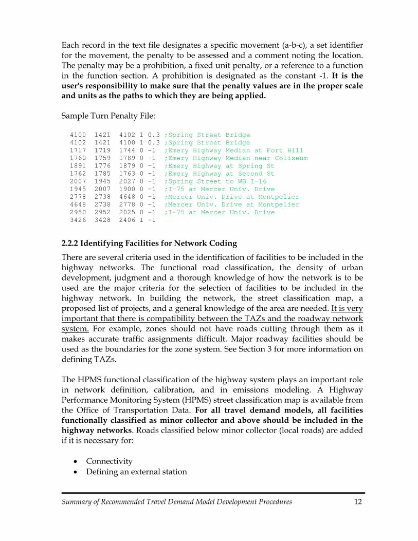
Summary of Recommended Travel Demand Model Development Procedures 12
Each record in the text file designates a specific movement (a-b-c), a set identifier for the movement, the penalty to be assessed and a comment noting the location. The penalty may be a prohibition, a fixed unit penalty, or a reference to a function in the function section. A prohibition is designated as the constant -1. It is the user's responsibility to make sure that the penalty values are in the proper scale and units as the paths to which they are being applied. Sample Turn Penalty File: 4100 1421 4102 1 0.3 ;Spring Street Bridge 4102 1421 4100 1 0.3 ;Spring Street Bridge 1717 1719 1744 0 -1 ;Emery Highway Median at Fort Hill 1760 1759 1789 0 -1 ;Emery Highway Median near Coliseum 1891 1776 1879 0 -1 ;Emery Highway at Spring St 1762 1785 1763 0 -1 ;Emery Highway at Second St 2007 1945 2027 0 -1 ;Spring Street to WB I-16 1945 2007 1900 0 -1 ;I-75 at Mercer Univ. Drive 2778 2738 4648 0 -1 ;Mercer Univ. Drive at Montpelier 4648 2738 2778 0 -1 ;Mercer Univ. Drive at Montpelier 2950 2952 2025 0 -1 ;I-75 at Mercer Univ. Drive 3426 3428 2406 1 -1
2.2.2 Identifying Facilities for Network Coding
There are several criteria used in the identification of facilities to be included in the highway networks. The functional road classification, the density of urban development, judgment and a thorough knowledge of how the network is to be used are the major criteria for the selection of facilities to be included in the highway network. In building the network, the street classification map, a proposed list of projects, and a general knowledge of the area are needed. It is very important that there is compatibility between the TAZs and the roadway network system. For example, zones should not have roads cutting through them as it makes accurate traffic assignments difficult. Major roadway facilities should be used as the boundaries for the zone system. See Section 3 for more information on defining TAZs. The HPMS functional classification of the highway system plays an important role in network definition, calibration, and in emissions modeling. A Highway Performance Monitoring System (HPMS) street classification map is available from the Office of Transportation Data. For all travel demand models, all facilities functionally classified as minor collector and above should be included in the highway networks. Roads classified below minor collector (local roads) are added if it is necessary for:
Connectivity Defining an external station
Summary of Recommended Travel Demand Model Development Procedures 13
It is known that a widening project or major development of regional impact (DRI) is planned in the future
“Regionally significant” facilities based on Interagency Consultation Process (used for Conformity Determination Reports)
A facility needed to load traffic out of a TAZ For future improvements, the projects typically come from the MPO’s planning process, but often additional projects will be outlined in SPLOST/1% Tax programs. Contact GDOT and the local governments to ensure that all planned transportation improvements are included in your project list.
3 Defining Traffic Analysis Zones
A fine Traffic Analysis Zone (TAZ) structure, provided the associated socio-economic data is accurate, helps to produce more accurate travel estimates at smaller geographic scales. But, the ability to accurately allocate socio-economic data to zones diminishes as zone size decreases (particularly for future forecasts). Refinement of TAZs is an important model component. Consultants working in these areas or developing models elsewhere in the state are suggested to coordinate with GDOT for any proposed changes or when defining TAZs for new models.
3.1 Creating Traffic Analysis Zones Most urban areas in Georgia have established TAZ boundaries, but when conducting a model update, existing boundaries should be evaluated and modified if needed. Areas that do not currently have travel demand models will need to establish TAZ boundaries, in cooperation with GDOT, during the model development process.
3.1.1 How to Select Appropriate TAZ Boundaries
It is important to establish zone boundaries that are appropriate for the purpose of the model. For example, appropriate zones for a statewide model may be census tracts, counties, or larger areas. A model for a corridor study may use very small zones. Urban area model zones generally fall somewhere in between. The ideal zone would serve:
The transportation planner as a suitable area for: o Travel demand modeling and analyses (including trip generation,
trip distribution, mode split, if applicable, and traffic assignment). o Quality control of demographics provided by planning agency
(zones aggregated to Census-defined units such as Block Groups, Tracts, and Census TAZs).
The planning agency:
Summary of Recommended Travel Demand Model Development Procedures 14
o As a suitable statistical unit for maintaining historical data. o As a unit of sufficient size to enable relatively accurate projection. o Preparation & quality control of demographics (zones aggregated to
Census units). o As an enumeration unit to be provided to the Census Bureau for the
next Census. Other uses by planning agency or participating units of government
Balancing these potentially competing desires leads to the need to establish priorities. As a result, GDOT recommends the following prioritized list of steps, which will be explained in more detail, for defining initial TAZ boundaries: 1. Ensure compatibility with appropriate US Census Bureau boundaries
(preferably those formed by roadways). 2. Include major topographic barriers as zone boundaries, such as large rivers or
major railroad lines. (These can be used in the determination of screenlines). 3. Use the modeled highway network when possible as zone boundaries, except
where undesirable zone boundaries would result (e.g. parallel screenlines). 4. Check for general zonal homogeneity (similar land use, density, socio-
economic attributes, etc.) and trip generating potential. In the case of mixed use development, zonal homogeneity is not possible. If the development is large enough, it should be considered a single zone in order to properly capture the intrazonal trips generated within the development. If the above priorities are observed, errors in traffic assignments are less likely to be attributable to zone boundary definitions. Although uncommon, it may be necessary to revise initial TAZ boundaries during model calibration and validation if isolated poor traffic assignments can be attributed to zone definitions.
3.1.2 Use of Census Information
In most areas, the only historical data for areas smaller than a political subdivision is that obtained through the Census Bureau. Because of this, geographic boundaries used by the Census Bureau have usually been used as the starting point for defining TAZ boundaries. This has facilitated updating and validating planning information using subsequent Census data. Figure 3-1 displays an example of the most common Census Bureau geographic units: Blocks, Block Groups, and Tracts. Census Blocks are the lowest level of Census geography. Blocks are combined to produce Block Groups. Block Groups are combined to produce Tracts.
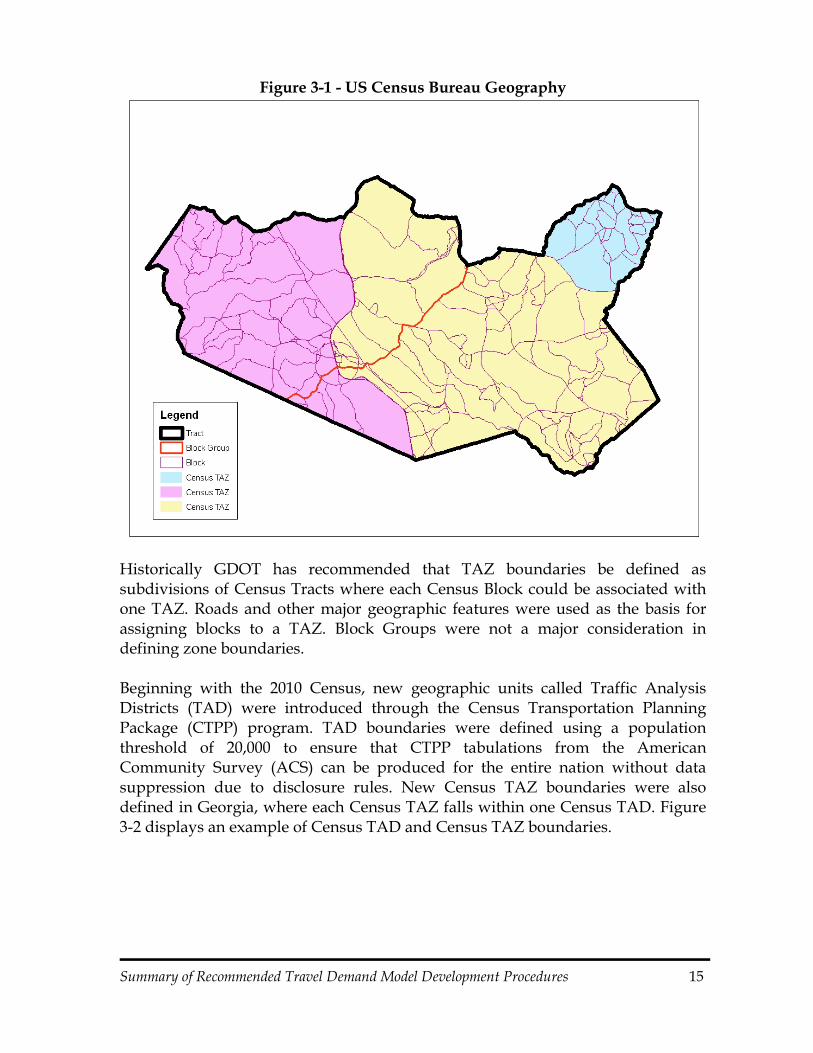
Summary of Recommended Travel Demand Model Development Procedures 15
Figure 3-1 - US Census Bureau Geography
Historically GDOT has recommended that TAZ boundaries be defined as subdivisions of Census Tracts where each Census Block could be associated with one TAZ. Roads and other major geographic features were used as the basis for assigning blocks to a TAZ. Block Groups were not a major consideration in defining zone boundaries. Beginning with the 2010 Census, new geographic units called Traffic Analysis Districts (TAD) were introduced through the Census Transportation Planning Package (CTPP) program. TAD boundaries were defined using a population threshold of 20,000 to ensure that CTPP tabulations from the American Community Survey (ACS) can be produced for the entire nation without data suppression due to disclosure rules. New Census TAZ boundaries were also defined in Georgia, where each Census TAZ falls within one Census TAD. Figure 3-2 displays an example of Census TAD and Census TAZ boundaries.
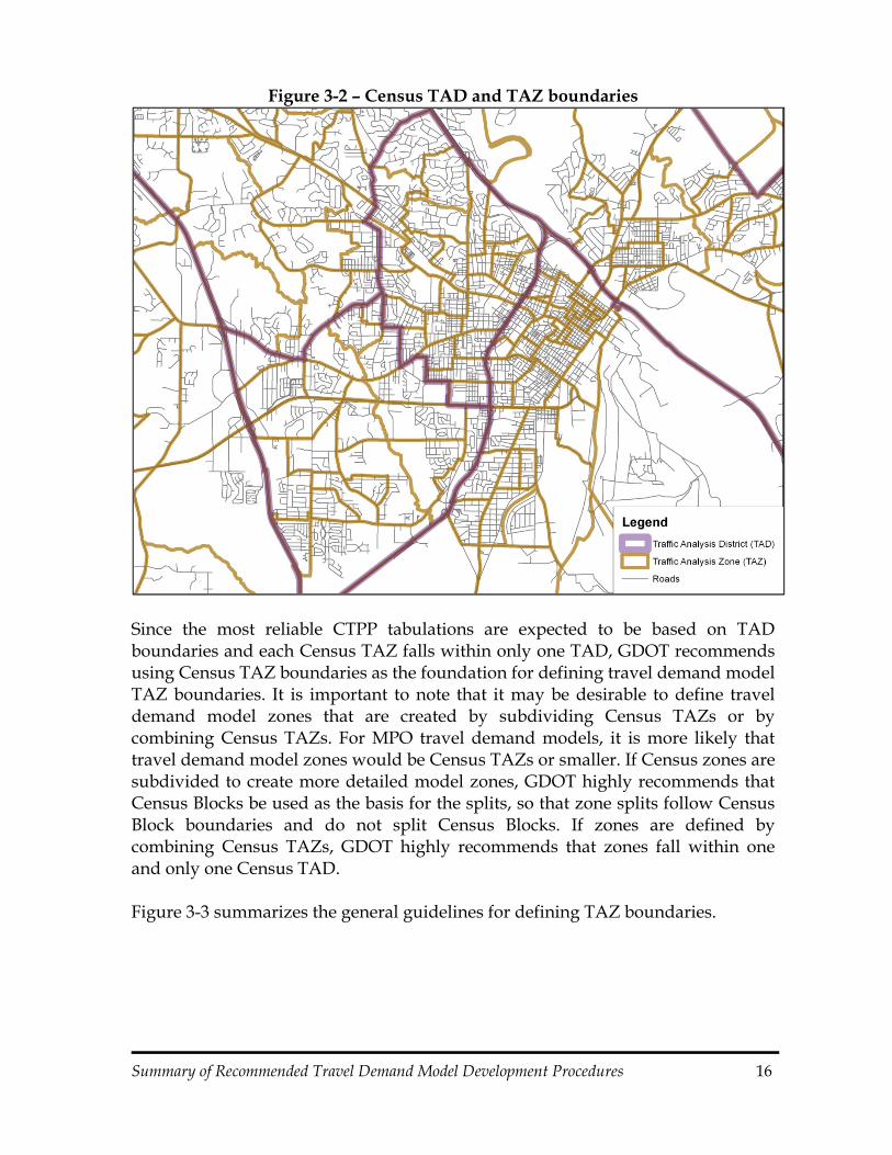
Summary of Recommended Travel Demand Model Development Procedures 16
Figure 3-2 – Census TAD and TAZ boundaries
Since the most reliable CTPP tabulations are expected to be based on TAD boundaries and each Census TAZ falls within only one TAD, GDOT recommends using Census TAZ boundaries as the foundation for defining travel demand model TAZ boundaries. It is important to note that it may be desirable to define travel demand model zones that are created by subdividing Census TAZs or by combining Census TAZs. For MPO travel demand models, it is more likely that travel demand model zones would be Census TAZs or smaller. If Census zones are subdivided to create more detailed model zones, GDOT highly recommends that Census Blocks be used as the basis for the splits, so that zone splits follow Census Block boundaries and do not split Census Blocks. If zones are defined by combining Census TAZs, GDOT highly recommends that zones fall within one and only one Census TAD. Figure 3-3 summarizes the general guidelines for defining TAZ boundaries.

Summary of Recommended Travel Demand Model Development Procedures 17
Figure 3-3 - Traffic Analysis Zone Guidelines
Local Geographic Information Systems (GIS) make it increasingly likely for local planning agencies to propose zones with boundaries NOT recognized by the U. S. Census Bureau. This is the case with most political subdivisions and with parcel-based mapping. To ensure consistency with the Census, GDOT recommends that zone boundary mapping conform to that recognized by the Census Bureau as previously described. Since Census Block Groups most often split tracts along streams rather than highways, they often do not form good TAZ boundaries for traffic assignment purposes and should be avoided.
3.1.3 Major Topographic Barriers
Screenlines should be identified using natural or constructed physical barriers, such as rivers, lakes, railroads, etc. These must cross the entire study area and may do so using combinations of barrier types. Barrier is the key here. These screenlines will be central to validating several modeling steps. Second only to Census TAZs, screenlines will form TAZ boundaries.
Summary of Recommended Travel Demand Model Development Procedures 18
TAZ boundaries should follow tangible physical features such as major roads, railroads, or rivers/streams. Major roads and railroads should be used as zone boundaries when possible (i.e., considering other guidelines such as not splitting Census Tracts).
3.1.4 Modeled Highway Network
It is desirable for the network to reflect, as much as possible, the area’s federal-aid functionally classified roadway system. Once the modeled highway network is defined, zones should be split progressively based on a hierarchy of roadway types until zone-network compatibility1 is achieved. The following hierarchy is recommended:
Define the Interstates/Freeways/Expressways as zone boundaries except where such divisions produce undesirable zones (e.g. bounded on three sides by railroads and on the fourth by a freeway, with no direct access).
Define the arterials as zone boundaries except where such divisions produce undesirable zones (e.g. narrow strip of right-of-way between a previously defined boundary such as a railroad serving as a screenline and a parallel major arterial).
Define the collectors as zone boundaries except where such divisions produce undesirable zones.
Define new location roadways under construction or having completed the environmental phase as zone boundaries. Although such roadways will not be reflected in the base year network, they will be in future system networks. Using these as zone boundaries will improve traffic assignment results. Boundaries along new location roadways should also be reflected in the next Census and will likely serve as a Census boundary in the future.
3.1.5 Zonal Homogeneity
Once zones are defined based on the modeled highway network, planners may further divide zones with socio-economic homogeneity as a goal. Areas that have similar trip-making characteristics (similar land uses, incomes, auto ownership levels, etc.) should be grouped together. This supports the statistical validity of several aspects of the travel demand modeling process. Generally, zonal homogeneity will not be attainable in the instance of mixed use developments. The following are typical factors in splitting zones for homogeneity purposes:
Population per acre (if possible, low density and high density areas should be in separate zones).
Occupied dwellings per structure (if possible, apartment areas should be separated from single unit areas).
1 Zone-Network Compatibility is generally achieved when no modeled roadways significantly bisect zones, except to avoid other undesirable modeling results. To do otherwise is not consistent with GDOT’s acceptable modeling procedures.

Summary of Recommended Travel Demand Model Development Procedures 19
Household income (if possible, low, middle, and high income areas should be separated).
Special major traffic generators, such as hospitals, shopping centers, etc., should be isolated into individual zones for specialized analysis.
Traffic zones with existing or future potential for generating a very high number of trips should be avoided. Zones that produce or attract too many trips can cause unreasonable spikes in loaded volumes where centroid connectors tie into the network.
Zone splits for homogeneity purposes should be along streets or along non-screenline topographic features such as streams or railroads. TAZ boundaries should not be assigned to dynamic jurisdictional lines such as city limits that do not abut other city limits. Fixed jurisdictional boundaries such as county lines or abutting city limits can be used, but are generally discouraged. Assigning TAZ boundaries to intangible arbitrary lines (e.g. property line defined solely by surveyed points) is highly discouraged and not supported by Census boundary parameters.
3.1.6 Other General Guidelines
A zone should have a symmetrical shape, avoiding narrow elongated, or “L” shapes. Elongated or “L” shaped zones make it difficult to properly assign trips onto the network with centroid connectors. Normally, zones are smaller in dense urban areas and larger in the outlying areas.
3.1.7 Estimated Number of Zones
The number of zones should be proportionate to the population. A rule-of-thumb that can be used to estimate the approximate number of TAZs for an urban area model is to take the square root of the study area population. Another commonly used rule of thumb recommends the number of zones be equal to the base year population divided by five-hundred. Table 3-1 displays the estimated number of zones for different population levels using these rules-of-thumb:
Table 3-1 - Rules of Thumb for Estimating Number of Traffic Zones Study Area Population
Estimated # Zones Pop^0.5
Estimated # Zones Pop/500
50,000 224 100 75,000 274 150 100,000 316 200 150,000 387 300 200,000 447 400 250,000 500 500 500,000 707 1000 750,000 866 1500
1,000,000 1000 2000

Summary of Recommended Travel Demand Model Development Procedures 20
3.1.8 Procedure for Numbering
A systematic methodology for numbering zones is desirable. Such a system enables the user to quickly locate a particular zone based on its number and relationship to the numbering pattern. It is recommended that the numbering system be prepared in consultation between the MPO and GDOT. Systematically numbered zones tend to:
Result in closer proximity of contiguously numbered zones; Enable the planner to more easily locate zones by proximity; and Improve the efficiency of network related computer processing.
Once the zones and external stations have been numbered, it is often desirable to insert a buffer between the last external station number and the first node number used in defining the roadway (traffic assignment) network. This buffer allows for future expansion of the study area and/or future subdivision of zones. Typically zone number one (1) is located in the CBD. It is recommended that planners develop a systematic numbering pattern for the rest of the study area’s zones. Using the predetermined pattern, assign a consecutive number to each traffic analysis zone. A common numbering pattern is to divide the study area into sectors or quadrants (e.g., CBD, NE, SE, SW, and NW). Once all of the zones in the CBD have been numbered, the modeler would move to the NE sector and begin number zones in a systematic manner, starting adjacent to the CBD. Once all the zones in the NE sector are numbered, the modeler would proceed in a clockwise direction to the SE sector and continue numbering zones beginning at the CBD and using consecutive numbers. This repeats, moving clockwise around the study area until all zones are numbered. A second zone numbering pattern is based on the geographical areas formed by the screenlines (which should be zone boundaries). One could concentrate numbering TAZs on one side of a screenline before moving to the other side with consecutive numbering. This would simplify identification of TAZ ranges for topographical penalties – if needed. A third numbering pattern is to number all the TAZs within a Census TAZ. Then move to the next TAZ within the same County. Continue this process until all TAZs in the County have been assigned a number. Later, external station numbers are assigned to the network’s roadways as they enter and exit the study area boundary. Although this cannot be done until the

Summary of Recommended Travel Demand Model Development Procedures 21
roadway network is defined, the numbering of external stations is dependent on the numbering of traffic analysis zones. Although not required, the first external station is often the next consecutive number following the last number used for traffic analysis zones. If a buffer of zones is desired between the last internal zones and the first external zone, it is advisable to insert “dummy2” zones in the network or specific steps taken in model scripts to ensure the gaps in TAZ numbering are properly treated. If the “clockwise” numbering procedure described above is used, the first external station to be numbered would be located in the northern part of the study area, near the last traffic analysis zone.
4 Socio-Economic Data
This section is intended to serve as a guide for preparing socio-economic data for Georgia’s regional travel demand models. This guide is intended for consultants or planners in MPOs that may not have established methodologies or are considering revising their current methodologies. Base year data produced by MPOs is critical for the calibration of the regional travel demand model. Figure 4-1 displays a generalized socio-economic data development process that is recommended by GDOT. This process can be applied in developing base year and future year data, although specific steps in the process may differ. This section provides an overview of a generalized data development process. To support the development and review of socioeconomic data, a review panel (i.e., MPO’s Transportation Coordinating Committee (TCC) and/or other local government technical personnel) should be formed. The purpose of the panel is to provide another level of review of control totals and the socio-economic data for reasonableness.
2 A “dummy” zone is a centroid in the network without associated socioeconomic data that is added to facilitate splitting zones for future corridor studies or adding zones for study area expansion. The zone must be added to the network and socio-economic files so that the modeling steps will run.

Summary of Recommended Travel Demand Model Development Procedures 22
Legen d
Travel Demand Model
Figure 4-1Generalized T ravel M odel Socio-Ec onomic Data Developmen t Proces s
U .S. Ce ns usPo p ula tion , Ho u se ho ld ,
an d In co m e D ataHo us ing Per mitA nd De m olitio n
D ata
Growth Trend s
A lloc ate Da ta toD istricts or T racts
If Av aila ble
La n d U se A cre ag eBy Ty pe b y TA Z
A lloc ate Da ta toT AZs
G row th in Re g io n al
Po p u la tio n &Ho u seh o lds
R eg ion a l Emp lo ym en tD ata by Ty pe
Lar ge Em plo ye rsB y Ty p e a nd Lo ca tion
(# Em p loy ee s)
Allo cate D ata toTAZs
G row th in Re gio n alEm plo ym e nt
By T yp e
Gro wth Tr ends
Em ploym en t Dat aBy Type b y TAZ
P opulation &Hou sehold Dat a by TAZ
EstimateMedian Inco me
Inp ut Data
Process - Res ultsAp prove d by GDOT
Proce ss - ResultsRev ie we d by GDOT
End Pro ducts
Figure 4-1 – Generalized Travel Model Socio-Economic Data Development Process
Summary of Recommended Travel Demand Model Development Procedures 23
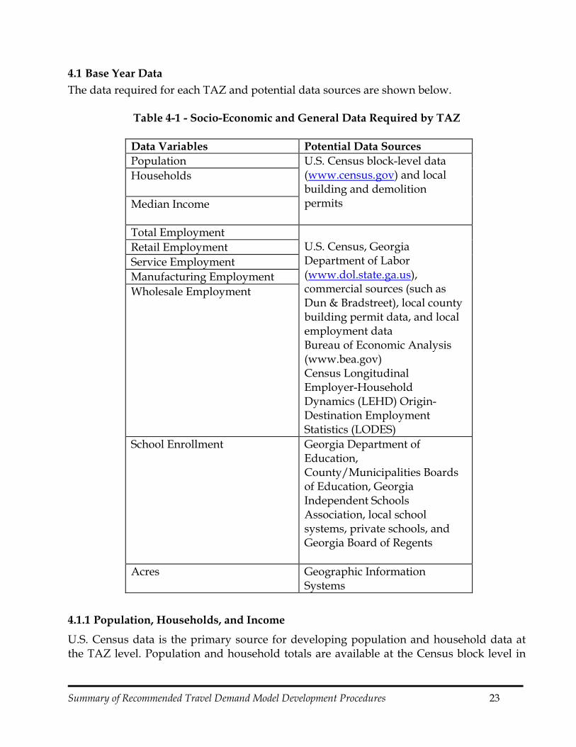
4.1 Base Year Data The data required for each TAZ and potential data sources are shown below.
Table 4-1 - Socio-Economic and General Data Required by TAZ
Data Variables Potential Data Sources Population U.S. Census block-level data
(www.census.gov) and local building and demolition permits
Households
Median Income
Total Employment U.S. Census, Georgia Department of Labor (www.dol.state.ga.us), commercial sources (such as Dun & Bradstreet), local county building permit data, and local employment data Bureau of Economic Analysis (www.bea.gov) Census Longitudinal Employer-Household Dynamics (LEHD) Origin-Destination Employment Statistics (LODES)
Retail Employment Service Employment Manufacturing Employment Wholesale Employment
School Enrollment Georgia Department of Education, County/Municipalities Boards of Education, Georgia Independent Schools Association, local school systems, private schools, and Georgia Board of Regents
Acres Geographic Information Systems
4.1.1 Population, Households, and Income
U.S. Census data is the primary source for developing population and household data at the TAZ level. Population and household totals are available at the Census block level in
Summary of Recommended Travel Demand Model Development Procedures 24
the Decennial Census. TAZ boundaries should not cross Census block boundaries, so estimation of population and household data are usually aggregation processes. Growth or decline that occurs between Census counts must be reflected in base year data (for base years between Census years). American Community Survey (ACS) provides 1 year, 3 year and 5 year estimates. TAZ specific adjustments can usually be made using local building and demolition permit data, supplemented by local knowledge of building activity. If building activity data is unavailable, planners should use a step-down estimation process. Begin by estimating the regional growth in population, then allocate that growth to planning districts (perhaps based on discussions with people who are knowledgeable of local building patterns), then further disaggregate the growth to TAZs. Existing land uses can be used as a basis for TAZ level allocation. Adjustments to population and households need to be taken for instances where group quarters exist. Common examples of this type of housing include prisons, hospitals, nursing homes and dormitories. While these group quarters have a distinct population, residents do not make trips in a typical fashion. For prisons and hospitals, the population should be removed from the socioeconomic data used in the modeling process. In other examples, a more representative population should be used to model the population utilizing the transportation network. In all of these examples, these group quarters should also correspond to a certain level of employment, e.g., hospital staff. In the case of a hospital, this employment will generate trips to the TAZ that is more representative of true conditions. Income data is available at the Census Tract (and Block Group) level. Since detailed income data is not available for smaller geographic areas, TAZ income data can be estimated from its associated Census Tract’s (or Block Group’s) data. Relatively large changes in development patterns (e.g., high cost homes constructed in a low income area) are usually necessary to produce significant changes in median income at the Census tract level. Such changes often occur slowly, so most TAZs will not require adjustments from Census income data. However, if specific TAZs have experienced considerable changes in development patterns since the last Census (e.g., new residential areas in a rural tract), some adjustments to income data are recommended.
4.1.2 Employment by Type
There are multiple sources of employment data. The Georgia Department of Labor (GDOL) provides county profiles and other reports that include county employment totals by employment class3. The US Census Bureau produces County Business Patterns reports, which provide employment by type at the county level. The US Department of Commerce Bureau of Economic Analysis (BEA) produces county employment estimates by North American Industry Classification System (NAICS) categories that should be used as control totals for Georgia MPO models. County level employment data can be downloaded from
3 http://explorer.dol.state.ga.us/mis/profiles.htm
Summary of Recommended Travel Demand Model Development Procedures 25
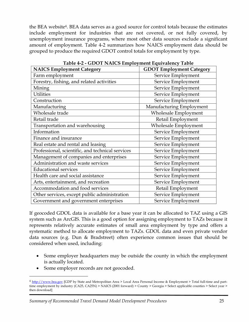
the BEA website4. BEA data serves as a good source for control totals because the estimates include employment for industries that are not covered, or not fully covered, by unemployment insurance programs, where most other data sources exclude a significant amount of employment. Table 4-2 summarizes how NAICS employment data should be grouped to produce the required GDOT control totals for employment by type.
Table 4-2 - GDOT NAICS Employment Equivalency Table NAICS Employment Category GDOT Employment Category Farm employment Service Employment Forestry, fishing, and related activities Service Employment Mining Service Employment Utilities Service Employment Construction Service Employment Manufacturing Manufacturing Employment Wholesale trade Wholesale Employment Retail trade Retail Employment Transportation and warehousing Wholesale Employment Information Service Employment Finance and insurance Service Employment Real estate and rental and leasing Service Employment Professional, scientific, and technical services Service Employment Management of companies and enterprises Service Employment Administration and waste services Service Employment Educational services Service Employment Health care and social assistance Service Employment Arts, entertainment, and recreation Service Employment Accommodation and food services Retail Employment Other services, except public administration Service Employment Government and government enterprises Service Employment
If geocoded GDOL data is available for a base year it can be allocated to TAZ using a GIS system such as ArcGIS. This is a good option for assigning employment to TAZs because it represents relatively accurate estimates of small area employment by type and offers a systematic method to allocate employment to TAZs. GDOL data and even private vendor data sources (e.g. Dun & Bradstreet) often experience common issues that should be considered when used, including:
Some employer headquarters may be outside the county in which the employment is actually located.
Some employer records are not geocoded.
4 http://www.bea.gov [GDP by State and Metropolitan Area > Local Area Personal Income & Employment > Total full-time and part-time employment by industry (CA25, CA25N) > NAICS (2001 forward) > County > Georgia > Select applicable counties > Select year > then download]

Summary of Recommended Travel Demand Model Development Procedures 26
Some records may be grouped to an arbitrary location within the county when the address could not be geocoded.
There may be some duplication of records. GDOL data does not include sole proprietorships or other classes of employment
that are not covered by unemployment compensation through the state. In each instance these items will need to be checked to determine if the GDOL data or geocoding need to be modified to correctly represent the amount and location of employment within the county. Employment for large employers and the geocoded location of large employers should be verified because they have significant potential influence on work trips. Employment for school districts should be checked to ascertain that it represents employment at individual schools rather than just the school district headquarters location. Census Longitudinal Employer-Household Dynamics (LEHD) Origin-Destination Employment Statistics (LODES) serves as a useful source for employment by type for small areas, when DOL data is unavailable. LODES employment data is available at the Census Block level, but it should not be used or applied at such small geographies due to methods that are employed to produce the data. It is reasonable to accumulate LODES data for all Census Blocks that are within a TAZ to estimate TAZ level employment data, however. As with all small area employment data sources, LODES data summarized at the TAZ level should be reviewed for reasonableness, including the issues previously described regarding GDOT and private vendor data. If small area employment data is unavailable, TAZ estimates should be developed using a step-down process. The largest employers in a county should be identified and employment totals (by category) assigned to their respective TAZ. Employment is then allocated to TAZs based on each TAZ’s share of the county’s corresponding land use category5. Retail employment can be allocated based on a TAZ’s share of the county’s commercial land use acreage. Service employment can be allocated based on a TAZ’s share of the commercial and residential acreage. Manufacturing employment can be allocated based on a TAZ’s share of the county’s industrial land use acreage. Wholesale employment can be allocated based on a TAZ’s share of the county’s industrial and commercial acreage. Residential acreage can be used in conjunction with Census data to allocate county population to TAZs (particularly in future allocation). Rural/vacant developable acreage and un-developable acreage is useful in determining developable acreage for each TAZ (i.e., subtracting from total acreage). Developable acreage can serve as a weighting factor for data allocation (growth from the base year to the future year). A step-down process can also begin with exogenously estimated district-level employment control totals. Then the previously described step-down process could be applied within each district separately, instead of the county-level.
5 Future data development can be supported by similar land use acreage assignments based on proposed future land use plans.

Summary of Recommended Travel Demand Model Development Procedures 27
Table 4-3 - Potential TAZ Land Use Database Variables
4.1.3 School Enrollment
It is preferable to obtain enrollment totals for each school in the study area (Elementary, Middle, High School, Private Schools, Technical Schools, Colleges, and Universities). If individual enrollments are not available, then system-wide totals by type of school could be an option. When combined with a comprehensive list of schools, an average school size could be calculated and allocated to each school (by type) equally. School enrollments should be available from school systems or through directly contacting individual schools. However, other potential data sources also exist, such as the State Board of Education, the Georgia Department of Technical and Adult Education, or the State Board of Regents.
4.1.4 Acres
TAZ acreage can be estimated best using GIS. MPOs should each maintain a GIS layer for TAZ boundaries. A regularly maintained land use database would also assist in developing consistency in socio-economic data estimates.
4.2 Future Year Projections All MPOs are encouraged to consider future land use plans and significant infrastructure changes (sewer extensions, new highway access, economic development plans, etc.) into future long-range socio-economic forecasts. The first step in developing future year projections is estimating regional population growth. Control totals for other forecast variables can be estimated based on the projected growth rate in population. For example, future total employment can be estimated by multiplying the base year ratio of employment and population to the projected population. The socio-economic data committee could provide guidance on shifts in the employment base that may need to be applied to future employment totals by type (e.g., reflect national trends of shifting to a more service oriented economy). Future school enrollment control
Total Acres Existing Commercial Acres Existing Residential Acres (best if stratified into density classes) Existing Industrial Acres Existing Rural/Vacant Developable Acres Undevelopable Acres Future Commercial Acres Future Residential Acres (best if stratified into density classes) Future Industrial Acres Future Rural/Vacant Developable Acres

Summary of Recommended Travel Demand Model Development Procedures 28
totals (by type of school) can be estimated using the base year ratio of enrollment and population. Average enrollments can then be allocated to schools by type. Unless significant changes in unemployment rates and age distributions are expected, assuming employment and school enrollments follow the growth in population should be sufficient for transportation planning purposes. There are many methods (and assumptions) for projecting population. Each MPO is responsible for developing future population forecasts. GDOT is responsible for ensuring that growth forecasts are reasonable. Prior to allocating future projections to TAZs, MPOs should provide GDOT documentation of the process and assumptions for their growth forecasts. GDOT conducts reasonableness checks on county population growth forecasts. Reasonableness checks will compare MPO forecasts to population projections using various methods (linear, exponential, share, etc.). If MPO forecasts are substantially different from GDOT’s expectations, GDOT will work with the MPO to resolve any disparities. There are many approaches to developing socio-economic data for travel demand models. This section provides relatively simple approaches for developing data. Provided below are simplified descriptions of the approaches that have been presented.
4.2.1 Population and Households
Primary data source: Existing US Census block-level data for distribution Assign each block to a TAZ Aggregate block-level data to produce TAZ-level Census data If the base year is different than the Census:
o Estimate growth in population & households since the last Census o Allocate the growth in population & households using share of residential
acreage (perhaps weighted by district or area type) or some other rational process
Collect county growth forecasts from the Georgia Office of Planning and Budget (OPB) to use as a potential guide or MPO growth forecasts from GDOT’s REMI model
Socio-economic data review panel reviews data and recommends appropriate modifications
Submit base year population and households data for use in developing the travel demand model to GDOT for review (if GDOT is responsible for building the model)
Develop and document the future regional projection methodology Socio-economic data review panel reviews methodology and projections and
recommends appropriate modifications Submit projection methodology and proposed control totals to GDOT GDOT concurs or works with the MPO to reach an agreement on the methodology
and control totals Allocate future population growth to TAZs
Summary of Recommended Travel Demand Model Development Procedures 29
Socio-economic data review panel reviews data and recommends appropriate modifications (may include multiple growth scenarios – at the discretion of the MPO and the data review panel)
Submit future year data for developing the future year travel models to GDOT for review (if GDOT is responsible for building the model)
4.2.2 Median Income
Primary source: US Census Tract or Block Group level data Assign each TAZ to a Tract or Block Group Assign the Census median income to each TAZ If the base year is different than the Census (or for future data):
o Estimate the share of new households that fall within each income group (likely based on tract or planning level assumptions and/or local knowledge of specific new developments).
o Estimate the median income by calculating a weighted average of the Census data and the assumed distribution of new households.
o Income should be reported in 2010 dollars.
4.2.3 Employment by Type
Primary data sources: o Bureau of Economic Analysis (BEA) o Georgia Department of Labor (supplemented with County Business Patterns,
private vendor sources, etc.) o Census Longitudinal Employer-Household Dynamics (LEHD) Origin-
Destination Employment Statistics (LODES) Assign the employment data to their respective TAZs based on the latitude and
longitude coordinates, if available (i.e. geocode) Geocode or aggregate small area employment data to TAZs and review for
reasonableness Identify the area's largest employers, determine employment levels for them, and
categorize the employment by type Assign the largest employers’ data to their respective TAZs Subtract the largest employers from the county-level data If small area employment data is unavailable, allocate the remaining employment
using the share of appropriate land-use acreage (perhaps weighted by district or area type) or some other rational process
o Employment Class and Potential Associated Land Use Categories Retail – Commercial Service – Commercial & Residential Manufacturing – Industrial Wholesale – Industrial & Commercial
Socio-economic data review panel reviews data and recommends appropriate modifications

Summary of Recommended Travel Demand Model Development Procedures 30
Submit base year employment data for use in developing the travel demand model to GDOT for review (if GDOT is responsible for building the model)
Estimate future employment control totals as a function of projected population growth and projected shifts in the economic base of the region
Socio-economic data review panel reviews employment projections and recommends appropriate modifications
Submit employment projection assumptions and proposed control totals to GDOT GDOT concurs or works with the MPO to reach an agreement on the assumptions
and control totals Allocate future employment growth to TAZs Socio-economic data review panel reviews data and recommends appropriate
modifications (may include multiple growth scenarios – at the discretion of the MPO and the data review panel)
Submit future year data for GDOT review and use in developing the future year travel models
4.2.4 School Enrollment
Primary data sources: Local school boards, private schools, State Board of Education, State Board of Regents, and the Georgia Department of Technical and Adult Education.
Manually assign school enrollment data to TAZs If specific school enrollments are unavailable:
o Obtain school system total enrollments by type of school o Obtain lists of schools and assign each school to its appropriate TAZ o Determine the number of schools by type and calculate an average school size
by type o Assign the average number of students in each school by type to each
school’s TAZ Ensure TAZ service employment is reasonable for zones with schools to account for
employment at schools
4.2.5 Acres
Develop a GIS-based TAZ layer and calculate total acres using the geography of the zones (if possible determine and report the total acreage that is developable and undevelopable)
4.3 Procedures to Check the Socio-Economic Data
4.3.1 Population per Household Ratio
Generally does not exceed 7 persons per household. o Anything over 7 persons per household should be explainable by some form
of group housing within the TAZ. o Do not include population in hospitals, nursing homes, and prisons since the
people who reside in these facilities are not making trips on the network.

Summary of Recommended Travel Demand Model Development Procedures 31
These populations are removed from the TAZ. For these types of businesses, the employment alone will reasonably generate the trips associated with these facilities.
Will decrease gradually over time, but not more than a few tenths. A drop of more than 0.5 persons per household over a 20 year span is significant.
Will typically be greater in suburban counties than in the center of a city. Is not less than 1.0 – this would correspond to a household that has no population
which by definition does not exist (household is a populated home).
4.3.2 Households (Occupied)
Do not decrease from existing to future projections without an explainable reason (e.g., redevelopment of a residential area into a commercial property – not a common occurrence).
Change in households should show a similar pattern to change in population.
4.3.3 Households per Acre
Over 4 households per acre would represent multifamily housing. Multifamily housing is typically located nearby a higher functional classification road (i.e., they are not generally located in rural or isolated areas).
Over 6 households per acre would signify multistory buildings. Again, check location for reasonableness.
4.3.4 Employment
About half of the available land can generally be considered for the building. Use the following to see if the size of the building is in line with the acreage of the TAZ. Include households as well (4 households per acre unless it is multifamily).
o Office 250 square feet per employee o Retail 300 square feet per employee o Wholesale 700 square feet per employee o Manufacturing 700 square feet per employee
4.3.5 Workforce Utilization
Ratio of Population to Employees generally stays constant. There should not be a significant change.
4.3.6 Income
Generally does not change. Keep in similar dollars for future forecasts. Do not adjust for inflation.
4.3.7 School Enrollment
School enrollment is generally around 20% of population. This number may be higher if there are large universities within the region.
The ratio of school enrollment to population should remain relatively similar from the base to future year.
Summary of Recommended Travel Demand Model Development Procedures 32
5 External Model Development
The following list briefly outlines some of the key steps recommended by GDOT to create a new external trip model for a base year model. 1. Identify the external stations for the model. Include all federal and state routes and also
include other significant county and city routes. Also review adjacent MPO or model boundaries for consistency between facilities.
2. Identify the GDOT coverage count station that is closest to the boundary of the model
for each external station. The coverage count station identified for each external station may or may not be located in the same county as the model.
3. Obtain the base year average daily traffic (ADT) for each external station from the
GDOT coverage count database. If an external station does not have a coverage count, assume an appropriate daily volume based on functional classification and location.
4. Identify the functional classification for each external station facility, as defined by
GDOT. 5. Based on the functional classification of the external station facility, assume a truck
percentage. If available, use percent trucks from recent vehicle-classification counts. Truck percentages, where available are listed on GDOT’s web site.
6. Assume a percentage of external-external trips for each external station. The remainder
of the trips at the external station will be internal-external trips. 7. Check the results of the fratar model to confirm that there was adequate closure for each
of the external stations (i.e. the fratar volumes match the desired volumes). Also, list the top ten external-external trip exchanges for both the passenger car and truck trip tables and check to make sure that these trip exchanges make sense.
6 Trip Generation
GDOT maintains a default trip generation process. The process uses the following trip purposes for estimation of internal person trips:
Home Based Work (HBW) Home Based Other (HBO) Home Based Shopping (HBS) Non-Home Based (NHB)
In regions with a significant level of college and university enrollment, GDOT recommends also including a separate trip purpose for university trips.
Summary of Recommended Travel Demand Model Development Procedures 33
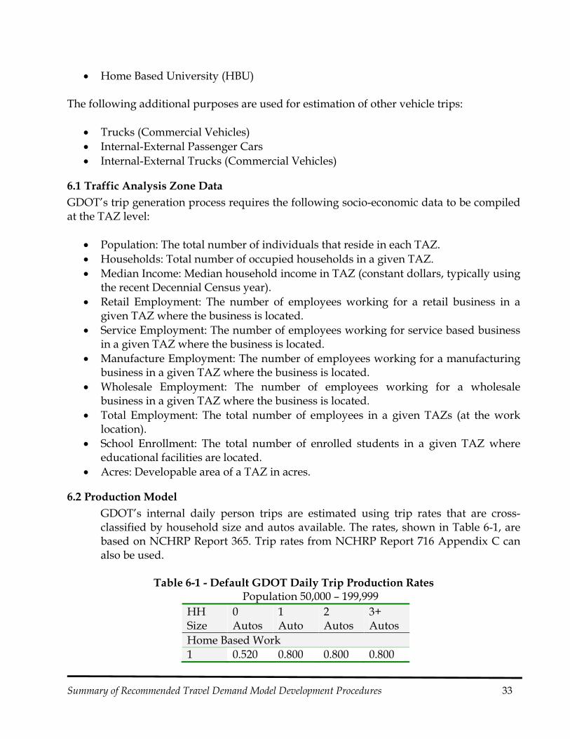
Home Based University (HBU)
The following additional purposes are used for estimation of other vehicle trips:
Trucks (Commercial Vehicles) Internal-External Passenger Cars Internal-External Trucks (Commercial Vehicles)
6.1 Traffic Analysis Zone Data GDOT’s trip generation process requires the following socio-economic data to be compiled at the TAZ level:
Population: The total number of individuals that reside in each TAZ. Households: Total number of occupied households in a given TAZ. Median Income: Median household income in TAZ (constant dollars, typically using
the recent Decennial Census year). Retail Employment: The number of employees working for a retail business in a
given TAZ where the business is located. Service Employment: The number of employees working for service based business
in a given TAZ where the business is located. Manufacture Employment: The number of employees working for a manufacturing
business in a given TAZ where the business is located. Wholesale Employment: The number of employees working for a wholesale
business in a given TAZ where the business is located. Total Employment: The total number of employees in a given TAZs (at the work
location). School Enrollment: The total number of enrolled students in a given TAZ where
educational facilities are located. Acres: Developable area of a TAZ in acres.
6.2 Production Model GDOT’s internal daily person trips are estimated using trip rates that are cross-classified by household size and autos available. The rates, shown in Table 6-1, are based on NCHRP Report 365. Trip rates from NCHRP Report 716 Appendix C can also be used.
Table 6-1 - Default GDOT Daily Trip Production Rates Population 50,000 – 199,999
HH Size
0 Autos
1 Auto
2 Autos
3+ Autos
Home Based Work 1 0.520 0.800 0.800 0.800
Summary of Recommended Travel Demand Model Development Procedures 34
HH Size
0 Autos
1 Auto
2 Autos
3+ Autos
2 1.056 1.474 1.782 1.848 3 1.406 1.748 2.014 2.261 4+ 1.800 2.160 2.520 2.880 Home Based Other 1 0.918 1.605 1.872 1.600 2 1.834 2.444 3.401 3.612 3 3.947 4.521 5.295 5.537 4+ 5.600 6.224 7.673 8.294 Home Based Shopping 1 0.486 0.555 0.288 0.560 2 0.758 1.174 0.973 0.924 3 0.197 0.631 0.641 1.127 4+ 0.400 0.976 0.727 1.306 Non-Home Based 1 0.676 1.040 1.040 1.040 2 1.152 1.608 1.944 2.016 3 1.850 2.300 2.650 2.975 4+ 2.200 2.640 3.080 3.520
Population 200,000-499,999
HH Size
0 Autos
1 Auto
2 Autos
3+ Autos
Home Based Work 1 0.420 0.860 0.860 0.860 2 0.920 1.449 1.725 1.725 3 1.320 1.936 2.332 2.860 4+ 1.350 2.160 2.520 2.880 Home Based Other 1 0.769 1.790 2.087 1.784 2 1.500 2.255 3.091 3.165 3 3.086 4.170 5.106 5.832 4+ 4.200 6.224 7.673 8.294 Home Based Shopping 1 0.407 0.618 0.321 0.624 2 0.620 1.084 0.884 0.810 3 0.154 0.582 0.618 1.188 4+ 0.300 0.976 0.727 1.306 Non-Home Based 1 0.504 1.032 1.032 1.032 2 0.960 1.512 1.800 1.800 3 1.440 2.112 2.544 3.120
Summary of Recommended Travel Demand Model Development Procedures 35
HH Size
0 Autos
1 Auto
2 Autos
3+ Autos
Home Based Work 4+ 1.650 2.640 3.080 3.520
Population 500,000 – 999,999
HH Size
0 Autos
1 Auto
2 Autos
3+ Autos
Home Based Work 1 0.575 1.058 1.058 1.058 2 1.056 1.608 1.872 1.872 3 1.288 2.024 2.392 2.783 4+ 1.425 2.280 2.660 3.040 Home Based Other 1 0.883 1.846 2.153 1.840 2 1.650 2.398 3.215 3.292 3 2.880 4.170 5.010 5.429 4+ 4.200 6.224 7.673 8.294 Home Based Shopping 1 0.467 0.638 0.331 0.644 2 0.682 1.153 0.919 0.842 3 0.144 0.582 0.606 1.105 4+ 0.300 0.976 0.727 1.306 Non-Home Based 1 0.575 1.058 1.058 1.058 2 1.012 1.541 1.794 1.794 3 1.288 2.024 2.392 2.783 4+ 1.575 2.520 2.940 3.360
Population 1,000,000+
HH Size
0 Autos
1 Auto
2 Autos
3+ Autos
Home Based Work 1 0.713 1.058 1.058 1.058 2 1.225 1.675 1.950 1.950 3 1.650 2.050 2.325 2.625 4+ 1.600 2.200 2.600 3.000 Home Based Other 1 1.014 1.710 1.993 1.704 2 1.803 2.353 3.154 3.229 3 3.269 3.742 4.314 4.536 4+ 4.480 5.705 7.125 7.776

Summary of Recommended Travel Demand Model Development Procedures 36
HH Size
0 Autos
1 Auto
2 Autos
3+ Autos
Home Based Shopping 1 0.536 0.590 0.307 0.596 2 0.745 1.131 0.902 0.827 3 0.163 0.522 0.522 0.924 4+ 0.320 0.895 0.675 1.224 Non-Home Based 1 0.837 1.242 1.242 1.242 2 1.127 1.541 1.794 1.794 3 1.518 1.886 2.139 2.415 4+ 1.600 2.200 2.600 3.000
6.2.1.1 Household Stratification Sub-Model
To apply cross-classified trip rates, the number of households in each cross-classification cell must be estimated. The household stratification model subdivides the total number of households by TAZ into 16 household strata defined by household size and the number of automobiles available. Stratification is done using TAZ median income, data from the Census Transportation Planning Package (CTPP), and data from the Augusta household survey. The model distributes the total households in a TAZ to each cross-classification cell by calculating a relative probability that a household will be a particular size with a particular number of automobiles. The relative probability is calculated with the following equation:
CFISjiP ),( where P(i, j) = Relative probability that a household will be size i and own j autos S = Household size factor from a lookup table I = Income factor from a lookup table CF = Composite household factor from Augusta household survey lookup table An estimate of the number of households in a particular cross-classification cell is then calculated by multiplying the total number of households in the TAZ by the corresponding relative probability. The final number of households in each cross-classification cell is calculated by applying a normalizing factor to each calculated value. The normalizing factor is applied to ensure that the sum of resulting disaggregated households equals the original aggregate number of households. This process is represented mathematically with the following equations:
),(.)( jiPHHestHH ij where
Summary of Recommended Travel Demand Model Development Procedures 37
.)(estHH ij = Estimated number of households of size i that own j autos
HH = Total number of households in the TAZ
FestHHHH ijij .)( where
ijHH = Final number of households of size i that own j autos
F = .)(/ estHHHH ij , control total normalizing factor
Examples of the three lookup tables used in the household stratification model are shown on the following pages. The current recommended lookup tables for household size and income were developed using CTPP 2000 data. In the future GDOT may update the lookup tables using newer Census data, but this is not urgent because the lookup tables follow logical progressions that are unlikely to change substantially. The current lookup tables have been reviewed to ensure that logical inconsistencies or discontinuities are not present. Household Size Distribution Summary of All Georgia Traffic Analysis Zones (CTPP 2000)
Computed Persons/HH Ranges (<=)
Household Size
1 2 3 4+ 0.0 1.0 1.0000 0.0000 0.0000 0.0000 1.0 1.2 0.7812 0.2056 0.0133 0.0000 1.2 1.4 0.6898 0.2568 0.0331 0.0203 1.4 1.6 0.5752 0.3128 0.0687 0.0433 1.6 1.8 0.4839 0.3511 0.1021 0.0630 1.8 2.0 0.4141 0.3537 0.1279 0.1043 2.0 2.2 0.3487 0.3563 0.1464 0.1486 2.2 2.4 0.2872 0.3471 0.1689 0.1968 2.4 2.6 0.2389 0.3274 0.1879 0.2458 2.6 2.8 0.1939 0.3140 0.1985 0.2935 2.8 3.0 0.1553 0.2947 0.2076 0.3424 3.0 3.2 0.1253 0.2749 0.2074 0.3924 3.2 3.4 0.1152 0.2489 0.1996 0.4363 3.4 3.6 0.1119 0.2116 0.1932 0.4832 3.6 3.8 0.1038 0.2042 0.1688 0.5232 3.8 4.0 0.1028 0.2032 0.1608 0.5332
Summary of Recommended Travel Demand Model Development Procedures 38
Typical Household Median Income Distribution Summary of All Georgia Traffic Analysis Zones (CTPP 2000)
TAZ-level Median HH Income Range
Income Group 1
Income Group 2
Income Group 3
Income Group 4
<$20,000 $20,000-$39,999
$40,000-$59,000 >=$60,000
$0 $2,500 0.8835 0.1165 0.0000 0.0000 $2,500 $5,000 0.8549 0.1168 0.0232 0.0050 $5,000 $7,500 0.8300 0.1318 0.0300 0.0081 $7,500 $10,000 0.7585 0.1468 0.0427 0.0521 $10,000 $12,500 0.6933 0.1826 0.0718 0.0523 $12,500 $15,000 0.6311 0.2131 0.0802 0.0756 $15,000 $17,500 0.5771 0.2465 0.0894 0.0870 $17,500 $20,000 0.5031 0.2938 0.1046 0.0985 $20,000 $22,500 0.4326 0.3321 0.1257 0.1096 $22,500 $25,000 0.3927 0.3387 0.1449 0.1236 $25,000 $27,500 0.3316 0.3581 0.1702 0.1401 $27,500 $30,000 0.3071 0.3488 0.1824 0.1617 $30,000 $32,500 0.2734 0.3395 0.1945 0.1926 $32,500 $35,000 0.2399 0.3356 0.2152 0.2093 $35,000 $37,500 0.2108 0.3322 0.2254 0.2316 $37,500 $40,000 0.1825 0.3143 0.2418 0.2615 $40,000 $42,500 0.1655 0.2840 0.2612 0.2893 $42,500 $45,000 0.1501 0.2688 0.2676 0.3134 $45,000 $47,500 0.1391 0.2550 0.2663 0.3396 $47,500 $50,000 0.1207 0.2387 0.2649 0.3758 $50,000 $52,500 0.1188 0.2142 0.2569 0.4101 $52,500 $55,000 0.1016 0.2012 0.2566 0.4407 $55,000 $57,500 0.0945 0.1894 0.2480 0.4682 $57,500 $60,000 0.0901 0.1853 0.2256 0.4990 $60,000 $62,500 0.0844 0.1684 0.2102 0.5371 $62,500 $65,000 0.0766 0.1598 0.2025 0.5612 $65,000 $67,500 0.0688 0.1510 0.1948 0.5854 $67,500 $70,000 0.0653 0.1416 0.1926 0.6004 $70,000 $72,500 0.0601 0.1271 0.1833 0.6295 $72,500 $75,000 0.0535 0.1218 0.1698 0.6549 $75,000 $77,500 0.0512 0.1087 0.1636 0.6765 $77,500 $80,000 0.0485 0.1042 0.1551 0.6922 $80,000 $82,500 0.0446 0.0991 0.1465 0.7099 $82,500 $85,000 0.0405 0.0939 0.1455 0.7202 $85,000 $87,500 0.0364 0.0889 0.1359 0.7387 $87,500 $90,000+ 0.0350 0.0839 0.1238 0.7573
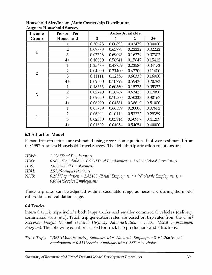
Summary of Recommended Travel Demand Model Development Procedures 39
Household Size/Income/Auto Ownership Distribution Augusta Household Survey
Income Group
Persons Per Household
Autos Available 0 1 2 3+
1
1 0.30628 0.66893 0.02479 0.00000 2 0.09778 0.65778 0.22222 0.02222 3 0.07326 0.69093 0.16279 0.07302
4+ 0.10000 0.56941 0.17647 0.15412
2
1 0.25483 0.47759 0.22586 0.04172 2 0.04000 0.21400 0.63200 0.11400 3 0.11111 0.12556 0.60333 0.16000
4+ 0.09000 0.10797 0.59420 0.20783
3
1 0.18333 0.60560 0.15775 0.05332 2 0.02740 0.16767 0.63425 0.17068 3 0.09000 0.10500 0.50333 0.30167
4+ 0.06000 0.04381 0.38619 0.51000
4
1 0.05769 0.66539 0.20000 0.07692 2 0.06944 0.10444 0.53222 0.29389 3 0.02000 0.05814 0.50977 0.41209
4+ 0.01892 0.04054 0.54054 0.40000
6.3 Attraction Model Person trip attractions are estimated using regression equations that were estimated from the 1997 Augusta Household Travel Survey. The default trip attraction equations are: HBW: 1.196*Total Employment HBO: 0.5077*Population + 0.967*Total Employment + 1.5258*School Enrollment HBS: 2.655*Retail Employment HBU: 2.5*off-campus students NHB: 0.293*Population + 2.82108*(Retail Employment + Wholesale Employment) +
0.6984*Service Employment These trip rates can be adjusted within reasonable range as necessary during the model calibration and validation stage.
6.4 Trucks Internal truck trips include both large trucks and smaller commercial vehicles (delivery, commercial vans, etc.). Truck trip generation rates are based on trip rates from the Quick Response Freight Manual (Federal Highway Administration - Travel Model Improvement Program). The following equation is used for truck trip productions and attractions: Truck Trips: 1.362*(Manufacturing Employment + Wholesale Employment) + 1.206*Retail
Employment + 0.514*Service Employment + 0.388*Households
Summary of Recommended Travel Demand Model Development Procedures 40
6.5 External Trips Traffic counts on highways that serve external trips (i.e., external stations) control the overall magnitude of external trips. Traffic at each external station is split into E-E passenger cars, E-E trucks, I-E passenger cars and I-E trucks. Assumed shares for external trip types are based on logical assignments. The share of E-E trips primarily depends on the facility type of the highway and its continuity with major highways that serve thru trips. Higher class roads with good thru trip connectivity will have higher E-E trip shares than lower class roads with lesser connectivity. Classification counts or typical vehicle type distributions are used to set passenger car and truck percents. It is possible using E-E trip shares and passenger car and truck shares to determine control totals for all external trip types. E-E trips are allocated to other external stations based on the magnitude of external trips at the potential destination and the distance between the stations. The higher the traffic count, the more likely it will attract E-E trips. The external trip estimation process assumes that the larger the distance between external stations, the higher the probability that trip interchange will serve E-E trips (i.e., since E-E trips travel completely thru the region, they are usually long distance trips). For I-E trips, it is necessary to estimate the internal location for the trip ends. This is done using the following regression equations: I-E Cars: 0.331*Households + 0.724*Total Employment I-E Trucks: 0.078*Retail Employment + 0.228*Manufacturing Employment + 2.149*Wholesale
Employment
6.6 Trip Generation Calibration/Validation GDOT calibrates andor validates model components by comparing model outputs to expected targets. Targets for various model parameters have been compiled from a number of sources. The following documents serve as the primary sources for checking the reasonableness of model parameters and results:
National Household Travel Survey (NHTS) 2009 - Georgia Add-On data National Cooperative Highway Research Program (NCHRP) Report 365 Travel Estimation
Techniques for Urban Planning NCHRP Report 716 Travel Demand Forecasting: Parameters and Techniques Model Validation and Reasonableness Checking Manual, TMIP, FHWA Travel Model Validation and Reasonability Checking Manual Second Edition, Travel Model
Improvement Program (TMIP), Federal Highway Administration (FHWA) Calibration and Adjustment of System Planning Models, USDOT, FHWA Quick Response Freight Manual, FHWA Quick Response Freight Manual II, FHWA
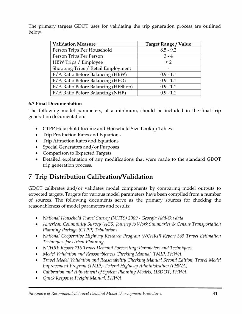
Summary of Recommended Travel Demand Model Development Procedures 41
The primary targets GDOT uses for validating the trip generation process are outlined below:
Validation Measure Target Range / Value Person Trips Per Household 8.5 - 9.2 Person Trips Per Person 3 - 4 HBW Trips / Employee < 2 Shopping Trips / Retail Employment - P/A Ratio Before Balancing (HBW) 0.9 - 1.1 P/A Ratio Before Balancing (HBO) 0.9 - 1.1 P/A Ratio Before Balancing (HBShop) 0.9 - 1.1 P/A Ratio Before Balancing (NHB) 0.9 - 1.1
6.7 Final Documentation The following model parameters, at a minimum, should be included in the final trip generation documentation:
CTPP Household Income and Household Size Lookup Tables Trip Production Rates and Equations Trip Attraction Rates and Equations Special Generators and/or Purposes Comparison to Expected Targets Detailed explanation of any modifications that were made to the standard GDOT
trip generation process.
7 Trip Distribution Calibration/Validation
GDOT calibrates and/or validates model components by comparing model outputs to expected targets. Targets for various model parameters have been compiled from a number of sources. The following documents serve as the primary sources for checking the reasonableness of model parameters and results:
National Household Travel Survey (NHTS) 2009 - Georgia Add-On data American Community Survey (ACS) Journey to Work Summaries & Census Transportation
Planning Package (CTPP) Tabulations National Cooperative Highway Research Program (NCHRP) Report 365 Travel Estimation
Techniques for Urban Planning NCHRP Report 716 Travel Demand Forecasting: Parameters and Techniques Model Validation and Reasonableness Checking Manual, TMIP, FHWA Travel Model Validation and Reasonability Checking Manual Second Edition, Travel Model
Improvement Program (TMIP), Federal Highway Administration (FHWA) Calibration and Adjustment of System Planning Models, USDOT, FHWA Quick Response Freight Manual, FHWA

Summary of Recommended Travel Demand Model Development Procedures 42
Quick Response Freight Manual II, FHWA The primary targets GDOT uses for validating the trip distribution process are outlined below:
Validation Measure Target Range / Value
Average Trip Length (HBW) Average Work Trip Time (CTPP / ACS)
+/- 5% Average Trip Length (HBO)
Set relative to the HBW target Average Trip Length (HBShop) Average Trip Length (NHB) Average Trip Length (Truck) N/A % Intrazonal Trips < 10%
GDOT uses average work trip length as the pivotal measure for calibrating distribution models. Target trip lengths for all internal person trip purposes are set based on the CTPP or ACS average work trip length. 6 Target non-work trip lengths are estimated using equations from Calibration and Adjustment of System Planning Models, NCHRP Report 365 and NCHRP Report 716. Calibration and Adjustment of System Planning Models includes equations to estimate average trip lengths based on the urban area population. NCHRP Report 365 includes an equation to estimate average work trip length based on the geographic size of the modeled area. NCHRP Report 365 and NCHRP Report 716 both provide common trip lengths for work and non-work trips which provides the relative length of non-work and work trips.
7.1 Final Documentation The following model parameters, at a minimum, should be included in the final trip distribution documentation:
CTPP Average Travel Time to Work Derivation of adjusted target average trip length targets Distribution parameters and resulting friction factor graphs Intrazonal time calculation methodology Terminal time assumptions Screenline maps and summaries Internal and external travel pattern spider webs Detailed explanation of any modifications that were made to the standard GDOT
trip distribution process.
6 If a significant share of external work trips is present in the census data, analysis of the census journey to work data may be necessary to estimate the intra-study area work trip length.
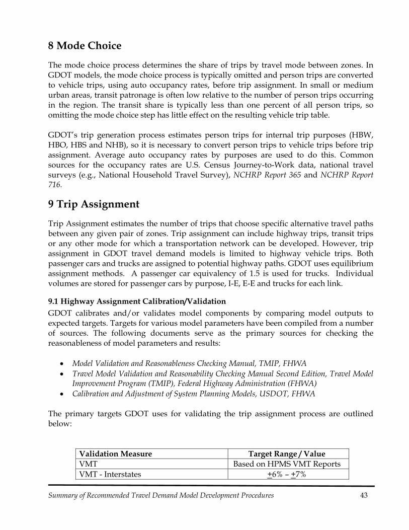
Summary of Recommended Travel Demand Model Development Procedures 43
8 Mode Choice
The mode choice process determines the share of trips by travel mode between zones. In GDOT models, the mode choice process is typically omitted and person trips are converted to vehicle trips, using auto occupancy rates, before trip assignment. In small or medium urban areas, transit patronage is often low relative to the number of person trips occurring in the region. The transit share is typically less than one percent of all person trips, so omitting the mode choice step has little effect on the resulting vehicle trip table. GDOT’s trip generation process estimates person trips for internal trip purposes (HBW, HBO, HBS and NHB), so it is necessary to convert person trips to vehicle trips before trip assignment. Average auto occupancy rates by purposes are used to do this. Common sources for the occupancy rates are U.S. Census Journey-to-Work data, national travel surveys (e.g., National Household Travel Survey), NCHRP Report 365 and NCHRP Report 716.
9 Trip Assignment
Trip Assignment estimates the number of trips that choose specific alternative travel paths between any given pair of zones. Trip assignment can include highway trips, transit trips or any other mode for which a transportation network can be developed. However, trip assignment in GDOT travel demand models is limited to highway vehicle trips. Both passenger cars and trucks are assigned to potential highway paths. GDOT uses equilibrium assignment methods. A passenger car equivalency of 1.5 is used for trucks. Individual volumes are stored for passenger cars by purpose, I-E, E-E and trucks for each link.
9.1 Highway Assignment Calibration/Validation GDOT calibrates and/or validates model components by comparing model outputs to expected targets. Targets for various model parameters have been compiled from a number of sources. The following documents serve as the primary sources for checking the reasonableness of model parameters and results:
Model Validation and Reasonableness Checking Manual, TMIP, FHWA Travel Model Validation and Reasonability Checking Manual Second Edition, Travel Model
Improvement Program (TMIP), Federal Highway Administration (FHWA) Calibration and Adjustment of System Planning Models, USDOT, FHWA
The primary targets GDOT uses for validating the trip assignment process are outlined below:
Validation Measure Target Range / Value VMT Based on HPMS VMT Reports VMT - Interstates +6% – +7%

Summary of Recommended Travel Demand Model Development Procedures 44
Validation Measure Target Range / Value VMT-Principal Arterials +10% - +15% VMT-Minor Arterials +10% - +15% VMT-Collectors +15% - +25% VMT-Total +5% VMT / Household VMT/ Person Screenlines All Counts
Maximum Desirable Deviation for Screenlines
& Individual Links
(NCHRP Report 255)
Screenline 1 Screenline 2 Screenline 3 Screenline 4 Screenline 5 RMSE = Root Mean Squared Error (Vol) < 30% AADT Volume Group: 0 - 5,000 < 100% AADT Volume Group: 5,001 - 10,000 < 75% AADT Volume Group: 10,001 - 15,000 < 50% AADT Volume Group: 15,001 - 20,000 < 30% AADT Volume Group: 20,001 - 30,000 < 30% AADT Volume Group: > 30,000 < 30%
GDOT recommends sensitivity tests be performed on the traffic assignment process. This can be done by comparing the assigned volumes before and after minor network modifications (e.g. adding a minor road widening or a single freeway ramp) are made. If minor network changes result in relatively significant fluctuations in volumes on links far from the network modifications, then the equilibrium assignment process has not reached an acceptable level of closure. Such hypersensitivity can usually be resolved by using more stringent closure criteria. GDOT recommends using a relative gap of 0.001 as the measure for equilibrium closure.
9.1.1 Poor Calibration Practices – What Not to Do
Although it is important to investigate why a travel demand model is poorly replicating individual counts, making isolated adjustments of individual link speeds, capacities or distances is usually inappropriate. Network corrections are appropriate, but artificial link-level adjustments are highly discouraged. Representing actual turn prohibitions in turn penalty files is appropriate. However, GDOT highly discourages the use of turn penalties to improve assignment results. Turn penalties can make a base year assignment appear to be valid, but many situations arise when it is
Summary of Recommended Travel Demand Model Development Procedures 45
unclear how turn penalties should be represented in future year applications. Liberal use of turn penalties also tends to create a less reliable traffic assignment process because problems that are more likely related to poor assignment parameters or network coding errors are masked by manual turn penalty adjustments. Model developers should focus model calibration efforts on using accurate data inputs (network coding, socio-economic data, etc.), reasonable model parameters and appropriate modeling procedures. If isolated traffic counts are poorly modeled, then model developers should ask why the model is not representing the situation well. Often such problems are a result of the size of zones, isolated high trip generators, the location of centroid connectors, incorrect socio-economic data, or any number of factors that should be investigated. Sometimes it is better to accept that the model cannot represent particular situations well rather than inserting ill-advised model adjustments just to make the assignment appear to be better.
9.1.2 Final Documentation
The following model parameters and results should be included in the final trip assignment documentation:
Speed and Capacity Assumptions Traffic Assignment scripts and a description of the parameters (closure criteria,
volume sets, link prohibitions, cost parameters, etc.) and characteristics (number of iterations to reach closure, iteration weights, etc.)
Volume-Delay Functions and Assignment Errors by Volume-Capacity Ratio Range Plots (for each Link Class)
Description of Turn Prohibitions VMT, Screenline and RMSE results Volume Bandwidth Plots (Maximum Desirable Deviation and Volume-Capacity
Ratios) Maximum Desirable Deviation Plot Volume versus Count Scatter Plot Plot(s) of congested speeds
10 Review of MPO Model Development Activities
If an MPO or a Consultant hired by an MPO is building a travel demand model that may be used in the development of the Long Range Transportation Plan (LRTP), GDOT recommends that the procedures discussed in the previous sections be used. If so desired, GDOT will review key steps in the development process to ensure that the model and model components meet GDOT’s recommended standards and guidance. GDOT review and/or the panel review is required on both the base and future year socio-economic data sets. It is recommended that two weeks being allowed for the review of each of the socio-economic data sets.

Summary of Recommended Travel Demand Model Development Procedures 46
11 File Naming Conventions
GDOT has instituted a file naming and folder protocol for the input and output files of the travel demand model set. The purpose of this effort is to ensure that there is consistency among MPOs with the various files and model runs. In addition, it assists with easy identification of the purpose or type of model file being reviewed. For example, a file with the extension of *.VTT is a vehicle trip table, whereas a file with the extension of *.PTT is a person trip table. The folder structure is displayed in Figure 11-1 while the file extensions protocols and folders are listed in Table 11-1.
Table 11-1 - Model File Naming Protocols Folder File Content File Name
Root Model script mpo{scenario}main.s Network display setting Default.vpr
Inputs
Input network mpo{scenario}.net SE data mpo{scenario}.dbf Turn penalty mpoturns{scenario}.pen External station mpo{scenario}.dbf
Parameters Base year vehicle trip table ttt2006.vtt Base year estimated vehicle trip table from matrix estimation estimate.vtt
Evaluation Screenline volume summary script Scrnline.s Cutline volume summary script Cutline.s
Scenario
Inputs
Parameters
Outputs
Evaluation
Matrix
Networks
Reports
Skims
Temp
Figure 11-1 – Model Folder Structure

Summary of Recommended Travel Demand Model Development Procedures 47
Folder File Content File Name
VMT summary script vmt.s
Maximum desired deviation summary script MaxDev.s/MaxDev.vpr (Base year only)
Outputs\Matrix
Gravity model vehicle trip table gmvol{scenario}.vtt
External-external passenger car vehicle trip table ee{scenario}.vtt (Table 1)
External-external truck vehicle trip table ee{scenario}.vtt (Table 2)
Total person trip table ptt{scenario}.ptt Total vehicle trip table ttt{scenario}.vtt
Outputs\Network Final loaded network mpo{scenario}_fin.lod
Outputs\Reports Program report files *.rpt
Turn output file turnmove{scenario}.trn Outputs\Skims Travel time skim time.skm
Outputs\Temp Model temporary files *.txt/*.hwy/*.lod
Note: mpo refers to the mpo such as BATS for Brunswick
12 Potential Treatment of Military Bases
There are two potential methods for estimating the impact of military bases on regional travel. One method is to treat the military base as a special generator and the other method is to create a separate trip purpose for the military employment. It is recommended that a separate trip purpose should be established for large military bases.
12.1 Treatment of Military Bases as Special Generators
12.1.1 Trip generation
One trip rate is usually applied to the military bases based on the military personnel on the base. It doesn’t differentiate between military and civilian population.
12.1.2 Trip distribution
Military trips are usually combined into the regular trip purposes such as, home-based work and home-based other for distribution. The distinct characteristics related to the travel pattern of the military personnel are not reflected. It is assumed that the civilian travel pattern also apply to military personnel. This might not always be true.
12.2 Treatment of Military Bases as a Separated Trip Purpose
12.2.1 Trip generation
Separate trip rates can be applied to military and civilian related activities based on the difference in the nature of the activities.

Summary of Recommended Travel Demand Model Development Procedures 48
12.2.2 Trip distribution
A separate gravity model can be applied to military purpose, providing a better handle on the trip distribution process. Military related personnel will go to military based employment, for example. The military personnel travel pattern can be represented in the distribution process. SE data requirement:
Military population and living quarters on the base Civilian population and households Military employment on the base Civilian employment on the base

Summary of Recommended Travel Demand Model Development Procedures 49
APPENDIX
Summary of Recommended Travel Demand Model Development Procedures 50
A-1: Socio-Economic Data Preparation Checklist and Review Guidelines The following guide is intended to assist Georgia MPOs with socioeconomic data forecasts for travel demand modeling purposes. These guidelines should be referred to after the MPO has projected future year socioeconomic data for the study area. The checks given below will help ensure that future year projections are consistent with base year conditions. Reliable socioeconomic data forecasts will contribute to a travel demand model that most accurately reflects future travel patterns and help the MPO develop sound long- and short-range plans. Some of these calculations are based on a traffic analysis zone (TAZ) level analysis, and others may be performed for the MPO as a whole. TAZ Level Analysis 1. Population to Household Ratio Calculation: Population / Number of Households Normally, the population to household ratio in each TAZ should not exceed 6.00 or 7.00. Ratios exceeding this amount should correspond to some type of group housing in the area – i.e., nursing home, dormitory, military barracks. The standard population to household ratio for each TAZ may be in the range of 2.00-3.00, but this may vary between each area. 2. Households per Acre Calculation: Number of Households / Acre Do not decrease number of households from existing to future projections without a reasonable explanation (e.g., redevelopment of a residential area into a commercial property-not a common practice). The number of households per acre in most TAZs should be less than 6.00. A value of 6.00 typically corresponds to a three-story multifamily building. Values exceeding 6.00 should accordingly correspond to larger or denser multifamily housing. 3. Population Relative to Acres Available Calculation: Population / Acre In each TAZ, the ratio of population to acres should not exceed 10.00. 4. Look for TAZs where households increase by greater than 500%.
Summary of Recommended Travel Demand Model Development Procedures 51
This percentage corresponds to a large increase in development activity. Ensure that TAZs that exceed this guideline are suitable for intense development. Examine suitability characteristics of the land, including flood hazard areas, wetlands, groundwater recharge, access to transportation networks, and access/proximity to future water and sewer services. 5. Note locations where wholesale employment is being allocated. Make sure that these
TAZs support this type of planned development. 6. Service Employment In TAZs that contain schools, there is typically one service employee to every 12 students. Divide the number of students (school enrollment) by the number of service employees allocated to the area and check whether the ratio is roughly equal to 12.00. If the ratio is significantly larger, then adequate service employment may not be allocated to that TAZ. 7. For each TAZ, the number of households should not decrease between the base year
and the future year. There are exceptions to this rule, for example, in areas undergoing urban renewal.
8. In each TAZ, make sure that the households have corresponding populations greater
than zero. Area Analysis 9. Employment Acres Calculation: Acres Available for Employment = [# acres – (# households / 4)] * 0.25 This calculation ensures that the projected number of acres needed for future employment will not be consumed by other uses. The equation first account for acreage taken up by future households, and it assumes that the remaining acreage is available for employment. The evaluation assumes that each household is comprised of a single-family home on a quarter-acre lot. Once you have found the number of acres needed for employment (according to the equation above), calculate how much acreage the future employment will consume. Allocate 0.00573921028 (250 square feet) acres of work space for each employee with the following equation: Acres Needed for Employment = (0.00573921028 acres / employee) * (# employees)

Summary of Recommended Travel Demand Model Development Procedures 52
The acres needed for employment should be less or equal to the acres available for employment. If this is not the case, then there may be certain TAZs (such as in downtown) that support multi-story office buildings and high density housing. If the value of acres available for employment (first calculation) is negative, this may be explained by denser housing (greater than 4 households per acre) or multifamily housing throughout the area. If either of the calculations produce negative numbers, make sure the figure is justified by higher densities of employment and/or housing than those that are assumed (4 households per acre and 250 square feet per employee). 10. School Enrollment School enrollment / population ≈ 20% Overall, the ratio of school enrollment to total population should be approximately 20%. This ratio may be higher due to universities or colleges in the area. 11. Make sure that the total number of households in the area is not decreasing between
the base year and the future year. An exception to this rule may be a large-scale urban renewal.
12. Note trends in future employment and changes in the types of households in the area.
For example, the center city is likely built out, so that drastic change is more difficult to accommodate.
13. The population to job ratio should be fairly constant over time (between the base and
future years). 14. Based on national trends, the population to household ratio in the area should decrease
slightly between the base and future years, with a future year value in the range of 2.8 – 2.9.
15. Note high-growth sectors in the study area, where population and households are
increasing by a large percentage. Examine the growth trend – is it consistent? See whether any TAZs are “skipped” along the trend area. Make sure that high growth areas are not already built out with housing and/or employment, and there is enough land to support the projected growth (examine parameters such as # households per acre).
What are the justifications for the high growth rate in these areas? These may include planned or emerging development in the area. Support the justifications with an examination of land suitability.
Summary of Recommended Travel Demand Model Development Procedures 53
A-2: Checklist for Preparing Highway Networks Update Previous Base Year Network Tasks
Review the GDOT construction lists (TransPI), consult with local jurisdictions and review aerials to determine highway improvements completed since the previous LRTP’s base year.
Review previous “Do-Nothing” and “E+C” networks to determine which network will serve as the best network from which to start creating the new base year network. Note that the “E+C” network may reflect several completed projects appropriate for the new base year, but might also require uncoding or removing some project improvements that were not complete at the time of the base year.
Add the completed highway improvements (projects) to whichever network is selected to serve as the basis for the new base year network.
Make sure that all functionally classified facilities minor collector and above are coded in the network. Use HPMS codes assigned by GDOT to each functionally classified roadway.
Make sure that if a road is used as a TAZ boundary the road is coded in the network.
If a road is not a TAZ boundary and functionally classified, this should send a red flag that either the road or the TAZ boundary needs review - (Ideally all functionally classified roads should be a TAZ boundary but sometimes that is not the case for a variety of reasons)
Update or add the functional classification (HPMS). If necessary, rename the old FCLASS or HPMS field to HPMS2000. New or newer models may need to have a HPMS2010 field added. Nonattainment Areas will most likely have both HPMS2000 and HPMS2010 fields.
Make sure if the road is being used a screenline/cutline, that the SCREENLINE and/or CUTLINE field(s) continues to be populated, if applicable.
Review traffic count station locations for accuracy and QA/QC the base year traffic count numbers
Add a new field and add the new traffic counts for the new base year that have undergone QA/QC. If necessary, rename the old traffic counts to Count {year} where {year} represents the 2 digit year of the last counts.
Use TIGER files as a background layer to improve the location of nodes and links Add road names if possible. Some of the older models may not have the field
ROADNAME populated. Add centroid connectors for new TAZs and revise existing centroid connector where
TAZs have been changed. When adding a new facility – the following attributes have to be populated for the
base year network.
o Number of Lanes o Facility type
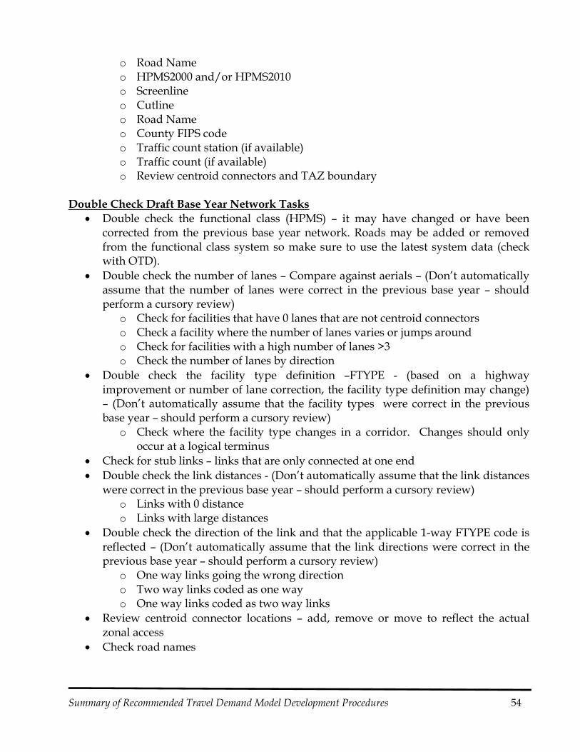
Summary of Recommended Travel Demand Model Development Procedures 54
o Road Name o HPMS2000 and/or HPMS2010 o Screenline o Cutline o Road Name o County FIPS code o Traffic count station (if available) o Traffic count (if available) o Review centroid connectors and TAZ boundary
Double Check Draft Base Year Network Tasks
Double check the functional class (HPMS) – it may have changed or have been corrected from the previous base year network. Roads may be added or removed from the functional class system so make sure to use the latest system data (check with OTD).
Double check the number of lanes – Compare against aerials – (Don’t automatically assume that the number of lanes were correct in the previous base year – should perform a cursory review)
o Check for facilities that have 0 lanes that are not centroid connectors o Check a facility where the number of lanes varies or jumps around o Check for facilities with a high number of lanes >3 o Check the number of lanes by direction
Double check the facility type definition –FTYPE - (based on a highway improvement or number of lane correction, the facility type definition may change) – (Don’t automatically assume that the facility types were correct in the previous base year – should perform a cursory review)
o Check where the facility type changes in a corridor. Changes should only occur at a logical terminus
Check for stub links – links that are only connected at one end Double check the link distances - (Don’t automatically assume that the link distances
were correct in the previous base year – should perform a cursory review) o Links with 0 distance o Links with large distances
Double check the direction of the link and that the applicable 1-way FTYPE code is reflected – (Don’t automatically assume that the link directions were correct in the previous base year – should perform a cursory review)
o One way links going the wrong direction o Two way links coded as one way o One way links coded as two way links
Review centroid connector locations – add, remove or move to reflect the actual zonal access
Check road names
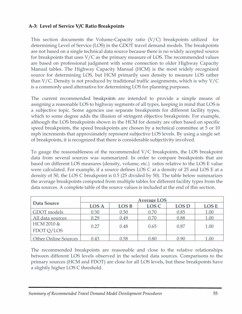
Summary of Recommended Travel Demand Model Development Procedures 55
A-3: Level of Service V/C Ratio Breakpoints
This section documents the Volume-Capacity ratio (V/C) breakpoints utilized for determining Level of Service (LOS) in the GDOT travel demand models. The breakpoints are not based on a single technical data source because there is no widely accepted source for breakpoints that uses V/C as the primary measure of LOS. The recommended values are based on professional judgment with some connection to older Highway Capacity Manual tables. The Highway Capacity Manual (HCM) is the most widely recognized source for determining LOS, but HCM primarily uses density to measure LOS rather than V/C. Density is not produced by traditional traffic assignments, which is why V/C is a commonly used alternative for determining LOS for planning purposes.
The current recommended breakpoints are intended to provide a simple means of assigning a reasonable LOS to highway segments of all types, keeping in mind that LOS is a subjective topic. Some agencies use separate breakpoints for different facility types, which to some degree adds the illusion of stringent objective breakpoints. For example, although the LOS breakpoints shown in the HCM for density are often based on specific speed breakpoints, the speed breakpoints are chosen by a technical committee at 5 or 10 mph increments that approximately represent subjective LOS levels. By using a single set of breakpoints, it is recognized that there is considerable subjectivity involved.
To gauge the reasonableness of the recommended V/C breakpoints, the LOS breakpoint data from several sources was summarized. In order to compare breakpoints that are based on different LOS measures (density, volume, etc.) ratios relative to the LOS E value were calculated. For example, if a source defines LOS C at a density of 25 and LOS E at a density of 50, the LOS C breakpoint is 0.5 (25 divided by 50). The table below summarizes the average breakpoints computed from multiple tables for different facility types from the data sources. A complete table of the source values is included at the end of this section.
Data Source
Average LOS LOS A LOS B LOS C LOS D LOS E
GDOT models 0.30 0.50 0.70 0.85 1.00 All data sources 0.29 0.49 0.70 0.88 1.00 HCM 2010 & FDOT Q/LOS H db k
0.27
0.48
0.65
0.87
1.00
Other Online Sources 0.43 0.58 0.80 0.90 1.00
The recommended breakpoints are reasonable and close to the relative relationships between different LOS levels observed in the selected data sources. Comparisons to the primary sources (HCM and FDOT) are close for all LOS levels, but these breakpoints have a slightly higher LOS C threshold.
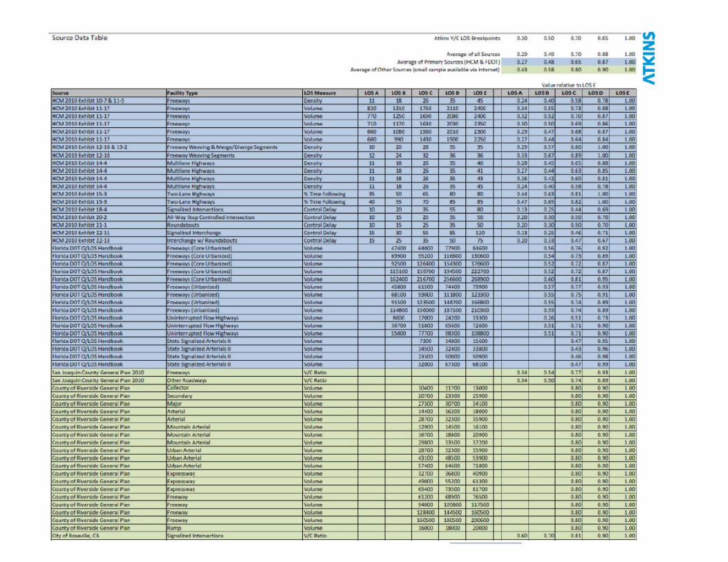
Summary of Recommended Travel Demand Model Development Procedures 56
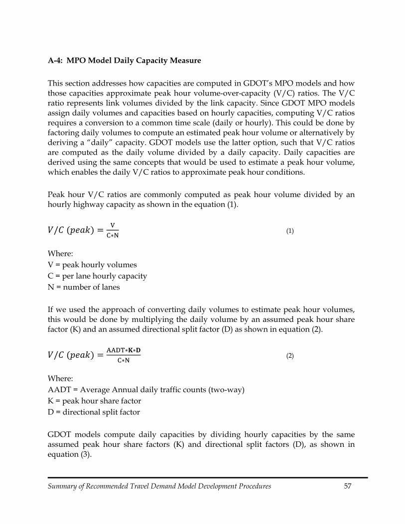
Summary of Recommended Travel Demand Model Development Procedures 57
A-4: MPO Model Daily Capacity Measure This section addresses how capacities are computed in GDOT’s MPO models and how those capacities approximate peak hour volume-over-capacity (V/C) ratios. The V/C ratio represents link volumes divided by the link capacity. Since GDOT MPO models assign daily volumes and capacities based on hourly capacities, computing V/C ratios requires a conversion to a common time scale (daily or hourly). This could be done by factoring daily volumes to compute an estimated peak hour volume or alternatively by deriving a “daily” capacity. GDOT models use the latter option, such that V/C ratios are computed as the daily volume divided by a daily capacity. Daily capacities are derived using the same concepts that would be used to estimate a peak hour volume, which enables the daily V/C ratios to approximate peak hour conditions. Peak hour V/C ratios are commonly computed as peak hour volume divided by an hourly highway capacity as shown in the equation (1).
/ ∗
(1)
Where: V = peak hourly volumes C = per lane hourly capacity N = number of lanes If we used the approach of converting daily volumes to estimate peak hour volumes, this would be done by multiplying the daily volume by an assumed peak hour share factor (K) and an assumed directional split factor (D) as shown in equation (2).
/ ∗ ∗
∗ (2)
Where: AADT = Average Annual daily traffic counts (two-way) K = peak hour share factor D = directional split factor GDOT models compute daily capacities by dividing hourly capacities by the same assumed peak hour share factors (K) and directional split factors (D), as shown in equation (3).
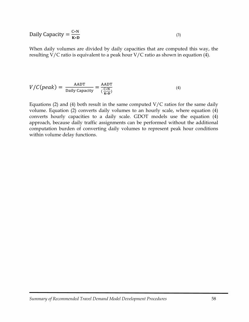
Summary of Recommended Travel Demand Model Development Procedures 58
DailyCapacity∗
∗ (3)
When daily volumes are divided by daily capacities that are computed this way, the resulting V/C ratio is equivalent to a peak hour V/C ratio as shown in equation (4).
/
∗ ∗
(4)
Equations (2) and (4) both result in the same computed V/C ratios for the same daily volume. Equation (2) converts daily volumes to an hourly scale, where equation (4) converts hourly capacities to a daily scale. GDOT models use the equation (4) approach, because daily traffic assignments can be performed without the additional computation burden of converting daily volumes to represent peak hour conditions within volume delay functions.
Summary of Recommended Travel Demand Model Development Procedures 59
GLOSSARY
Average Annual Daily Traffic (AADT) – The total amount of traffic observed, counted or estimated in both directions during a 24-hour period which has been averaged over the year. GDOT’s 445 reports summarize AADT by county. Average Daily Traffic (ADT) - The total amount of traffic observed, counted or estimated in both directions during a 24-hour period. Calibration – Process of adjusting constants and other model parameters in the development of the models so that the models replicate observed data for a base (calibration) year. Capacity - The maximum volume of travel that a transportation facility can accommodate during a specified time period such as hour, period or day. Centroid - A point that represents a TAZ that loads traffic onto the model network via centroid connectors. Centroids are typically placed so that they represent the approximate “center of mass” for trips generated by the TAZ. Cordon Lines – Lines that completely encompass a designated area. Cordon lines are typically associated with the boundary of the area being modeled. Usually used to validate travel movements. Frequently used to assess travel within the Central Business District (CBD). Cube Software – A travel demand modeling software package that GDOT uses. Cutlines - Cutlines extend across a corridor containing multiple facilities. They should be used to intercept travel along only one axis. Cutlines are used to look at particular locations and corridors. Equilibrium Highway Assignment - a method of traffic assignment where trips select the shortest path while considering the impacts of congestion, impedances and costs on travel time. Friction Factors - Parameters used in the Trip Distribution step of the model process. These are variables that quantify the impedance or measure of separation between two traffic analysis zones. Friction factors are inversely related to the spatial separation of zones, decreasing as impedance increases. The gravity model used in trip distribution method originally generated from an analogy with Isaac Newton’s gravitational law. This analogy posits that the interaction between two locations declines with increasing impedance (distance, time, and cost) between them, but is positively associated with the amount of activity at each location.
Summary of Recommended Travel Demand Model Development Procedures 60
Geographic Information Systems (GIS) - Computer software and databases that allow for the storage, retrieval and analysis of spatial information. High-Occupancy / Toll (HOT) - Policies that provide designated lanes on arterials and freeways that gives motorists in single-occupant vehicles access to high-occupancy vehicle lanes (or "HOV lanes"). High-Occupancy Vehicle (HOV) - Vehicles with a driver and one or more passengers. Policies are in place in some localities that provide dedicated arterial and freeway lanes that are reserved for vehicles with at least two occupants (driver and one or more passengers). Impedance – Various measures of cost (distance, time, transit fare, parking cost, etc.) used to estimate the interaction between two locations. K-Factors - A parameter used in trip distribution to adjust trip making interchanges between two subareas of the region, often thought of as a ”socioeconomic” adjustment that cannot otherwise be represented in the model. GDOT recommends that these parameters be used as a last resort in model development. (not to be confused with a peak hour share k-factor) Level of Service (LOS) - A qualitative measure of intersection or road segment operating condition. A grading scale of A through F is used to characterize traffic operating conditions. The scale is based on the ability of an intersection or street segment to accommodate the amount of traffic using it, and can be used for both existing and projected conditions. The scale ranges from “A” which indicates little, if any, vehicle delay, to “F” which indicates significant vehicle delay and traffic congestion. MPO (Metropolitan Planning Organization) - A required planning unit that all urban areas over 50,000 in population must have. Mode Choice – This step determines the mode of a trip based on socioeconomic characteristics of the traveler or households, auto occupancy and availability of modal options such as HOV lanes, Managed lanes and transit options. The characteristics of the travel network include level of service variables such as time, cost, and the number of transit transfers. Mode choice is usually modeled separately for each trip or tour purpose and is usually the third step in the modeling process. O-D (Origin-Destination) - refers to the beginning and ending of a trip. Root Mean Square Error (RMSE) – A measure of the differences between traffic volumes predicted by a model and the observed traffic counts.
Summary of Recommended Travel Demand Model Development Procedures 61
P-A (Production – Attraction) - Similar to O-D except that it refers to the trip ends. Trips are not linked by origin and destination zones. Percent Error – Shows the relative error between an observed traffic count and a model estimated traffic volume as a percentage. Person Trip – A one-way trip made by a person by any mode from an origin to a destination zone. Person trips are the usual units in transit assignment but person trips are converted to vehicle trips for highway assignment. Screenlines – Represent imaginary lines that are used to divide the study area into large sections to assess model validation. They extend completely across the modeled area from boundary cordon to boundary cordon and capture cross-regional travel flows. Screenlines are often associated with physical barriers such as rivers or railroads, although jurisdictional boundaries such as county lines that extend through the study area may also be used as screenlines. Comparison of modeled versus counted traffic across screenlines provides an indication of how well a travel demand model performs in replicating major trip patterns and movements throughout the network. Skim Matrix - A matrix with a measure of the shortest path between each pair of centroids or zones using either free-flow time, congested time or distance. Traffic Analysis Zones (TAZ or zone) – Basic unit of geography used in transportation planning models. The spatial extent of zones or TAZs varies in models based on area type with very large zones in rural or exurban areas while the size of the zones decrease as population and employment density increase. Socio-economic or demographic data such as population, number of households, number of automobiles per household, household income and employment by zone are prepared at this level. Trip Assignment – This involves assigning traffic to a transportation network which consists of roadways and in some cases, transit routes using a mathematical algorithm that determines the amount of traffic as a function of time, volume, capacity or impedance factor. This is usually the fourth step in the modeling process. Trip Attraction – The trip end of a home-base trip that occurs at the non-home location, or the destination end of a non-home-based trip. Trip Distribution – This step links tripmaker’s origins with their destinations by TAZ. It determines where people work, shop and perform other daily activities such as school, errand, entertainment etc. The trips are estimated based on a function of the attractiveness of a zone and the travel impedance between zones. This is usually the second step in the traditional four-step transportation modeling process.

Summary of Recommended Travel Demand Model Development Procedures 62
Trip Generation – The step in the modeling process where daily travel is estimated by zone which includes the trip purpose and amount of travel. Trips are estimated on the socioeconomic characteristics of the zone. This is usually the first step in the traditional four-step transportation modeling process. Trip Length Frequency Distribution – This is a curve that shows the distribution of model-estimated trip lengths by trip purpose. Trip Production – The trip end of home-based trip that occurs at the home, or the origin end of a non-home-based trip. Topo Penalty – A perceived value of time that is added to travel times between zones that cross physical barriers such as rivers, lakes, railroads. Turn Prohibitor – These are flags coded on intersections in the highway network that add impedances to travel time and movement where the travel movement is prohibited, such as the prohibition of a left-hand turn. V/C Ratio (Volume/Capacity Ratio) - Represents the vehicle flow on a roadway divided by the maximum flow capacity. If this equals one, the roadway is at capacity. Validation – Application of the calibrated models and comparison of the results with observed data in order to determine how well the models are replicating observed data for the base year. Vehicle Trip – A trip made by a motorized vehicle from an origin to a destination such as a passenger car, commercial vehicle or heavy duty truck. Vehicle trips are the usual units in highway assignments. VHT (Vehicle Hours Traveled) - A measure of vehicle travel time on a roadway or network of roadways. It is the sum of the vehicle travel time of all vehicles for a segment of roadway. For a given roadway VHT = Daily Volume * Time (in Minutes). VMT (Vehicle Miles Traveled) - A measure of vehicle travel on a roadway or network of roadways. It is the sum of the mileage driven of all vehicles for a segment of roadway. For a given roadway VMT = Daily Volume * Length (in Miles).