A nonconforming high-order method for the Biot problem ongeneral meshes

Daniele Boffi˚1, Michele Botti:1,2, and Daniele A. Di Pietro;2

1 Università degli Studi di Pavia, Dipartimento di Matematica “Felice Casorati”, 27100 Pavia, Italy2 University of Montpellier, Institut Montpéllierain Alexander Grothendieck, 34095 Montpellier,

France

June 12, 2015

Abstract

In this work, we introduce a novel algorithm for the Biot problem based on a HybridHigh-Order discretization of the mechanics and a Symmetric Weighted Interior Penaltydiscretization of the flow. The method has several assets, including, in particular, the sup-port of general polyhedral meshes and arbitrary space approximation order. Our analysisdelivers stability and error estimates that hold also when the specific storage coefficientvanishes, and shows that the constants have only a mild dependence on the heterogeneityof the permeability coefficient. Numerical tests demonstrating the performance of themethod are provided.

1 Introduction

We consider in this work the quasi-static Biot’s consolidation problem describing Darcian flowin a deformable saturated porous medium. Our focus is on applications in geosciences, wherethe support of general polyhedral meshes is crucial, e.g., to handle nonconforming interfacesarising from local mesh adaptation or Voronoi elements in the near wellbore region whenmodelling petroleum extraction; cf. Figure 1 for an example. Let Ω Ă Rd, 1 ď d ď 3, denote abounded connected polyhedral domain with boundary BΩ and outward normal n. For a givenfinite time tF ą 0, volumetric load f , fluid source g, the Biot problem consists in finding avector-valued displacement field u and a scalar-valued pore pressure field p solution of

´∇¨σpuq ` α∇p “ f in Ωˆ p0, tFq, (1a)c0dtp`∇¨pαdtuq ´∇¨pκ∇pq “ g in Ωˆ p0, tFq, (1b)

where c0 ě 0 and α ą 0 are real numbers corresponding to the constrained specific storage andBiot–Willis coefficients, respectively, κ is a real-valued permeability field such that κ ď κ ď κ

˚daniele.boffi@unipv.it:michele.botti01@universitadipavia.it;daniele.di-pietro@univ-montp2.fr

1

arX

iv:1

506.

0372

2v1

[m

ath.

NA

] 1

1 Ju

n 20

15

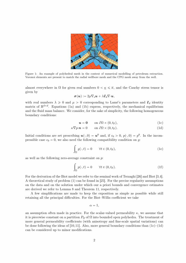
Figure 1: An example of polyhedral mesh in the context of numerical modelling of petroleum extraction.Voronoi elements are present to match the radial wellbore mesh and the CPG mesh away from the well.

almost everywhere in Ω for given real numbers 0 ă κ ď κ, and the Cauchy stress tensor isgiven by

σpuq :“ 2µ∇su ` λId∇¨u,with real numbers λ ě 0 and µ ą 0 corresponding to Lamé’s parameters and Id identitymatrix of Rdˆd. Equations (1a) and (1b) express, respectively, the mechanical equilibriumand the fluid mass balance. We consider, for the sake of simplicity, the following homogeneousboundary conditions:

u “ 0 on BΩˆ p0, tFq, (1c)κ∇p¨n “ 0 on BΩˆ p0, tFq. (1d)

Initial conditions are set prescribing up¨, 0q “ u0 and, if c0 ą 0, pp¨, 0q “ p0. In the incom-pressible case c0 “ 0, we also need the following compatibility condition on g:

ż

Ωgp¨, tq “ 0 @t P p0, tFq, (1e)

as well as the following zero-average constraint on p:ż

Ωpp¨, tq “ 0 @t P p0, tFq. (1f)

For the derivation of the Biot model we refer to the seminal work of Terzaghi [26] and Biot [3,4].A theoretical study of problem (1) can be found in [25]. For the precise regularity assumptionson the data and on the solution under which our a priori bounds and convergence estimatesare derived we refer to Lemma 8 and Theorem 11, respectively.

A few simplifications are made to keep the exposition as simple as possible while stillretaining all the principal difficulties. For the Biot–Willis coefficient we take

α “ 1,

an assumption often made in practice. For the scalar-valued permeability κ, we assume thatit is piecewise constant on a partition PΩ of Ω into bounded open polyhedra. The treatment ofmore general permeability coefficients (with anisotropy and fine-scale spatial variations) canbe done following the ideas of [10,11]. Also, more general boundary conditions than (1c)–(1d)can be considered up to minor modifications.

2

Several difficulties have to be accounted for in the design of a discretization methodsfor problem (1): in the context of nonconforming methods, the linear elasticity operatorhas to be carefully engineered to ensure stability expressed by a discrete counterpart of theKorn’s inequality; the Darcy operator has to accomodate rough variations of the permeabilitycoefficient; the choice of discrete spaces for the displacement and the pressure must satisfyan inf-sup condition to contribute reducing spurious pressure oscillations for small time stepscombined with small permeabilities when c0 “ 0. An investigation of the role of the inf-supcondition in the context of finite element discretizations can be found, e.g., in Murad andLoula [17, 18]. A recent work of Rodrigo, Gaspar, Hu, and Zikatanov [24] has pointed outthat, even for discretization methods leading to an inf-sup stable discretization of the Stokesproblem in the steady case, pressure oscillations can arise owing to a lack of monotonicity ofthe operator. Therein, the authors suggest that stabilizing is possible by adding to the massbalance equation artificial diffusion terms with coefficient proportional to h2τ (with h andτ denoting, respectively, the spatial and temporal meshsizes). However, computing the exactamount of stabilization required is in general feasible only in 1 space dimension.

The discretization of the Biot problem has been considered in several other works. Finiteelement discretizations are discussed, e.g., in the monograph of Lewis and Schrefler [16]; cf.also references therein. A finite volume discretization for the three-dimensional Biot problemwith discontinuous physical coefficients was considered by Naumovich [19]. In [21,22], Phillipsand Wheeler propose and analyze an algorithm that models displacements with continuouselements and the flow with a mixed method. In [23], the same authors also propose a differentmethod where displacements are instead approximated using discontinuous Galerkin methods.In [27], Wheeler, Xue and Yotov study the coupling of multipoint flux discretization for the flowwith a discontinuous Galerkin discretization of the displacements. While certainly effectiveon matching simplicial meshes, discontinuous Galerkin discretizations of the displacementsusually do not allow to prove inf-sup stability on general polyhedral meshes.

In this work, we propose a novel discretization of problem (1) where the linear elasticityoperator is discretized using the Hybrid High-Order (HHO) method of [9], while the flow relieson the Symmetric Weighted Interior Penalty (SWIP) discontinuous Galerkin method of [11,13];see also [8, Chapter 4]. The proposed method has several assets:(i) it delivers an inf-supstable discretization on general meshes including, e.g., polyhedral elements and nonmatchinginterfaces; (ii) it allows to increase the space approximation order to accelerate convergence inthe presence of (locally) regular solutions; (iii) it is locally conservative on the primal mesh;(iv) it is robust with respect to the spatial variations of the permeability coefficient, withconstants in the error estimates that depend on the square root of the heterogeneity ratio;(v) it is (relatively) inexpensive: at the lowest order, after static condensation of elementunknowns for the displacement, we have 4 (resp. 9) unknowns per face for the displacements+ 3 (resp. 4) unknowns per element for the pore pressure in 2d (resp. 3d). Finally, theproposed construction is valid for arbitrary space dimension, a feature which can be exploitedin practice to conceive dimension-independent implementations.

The material is organized as follows. In Section 2, we introduce the discrete setting,formulate the method, and investigate its local conservation properties by identifying theconservative normal tractions and mass fluxes. In Section 3, we derive a priori bounds on theexact solution for regular-in-time volumetric load and mass source. The convergence analysisof the method is carried out in Section 4. Finally, numerical tests are proposed in Section 5.

3

2 Discretization

In this section we introduce the assumptions on the mesh, define the discrete counterparts ofthe elasticity and Darcy operators and of the hydro-mechanical coupling terms, formulate thediscretization method and investigate its local conservation properties.

2.1 Mesh and notation

Denote by H Ă R` a countable set of meshsizes having 0 as its unique accumulation point.Following [8, Chapter 1], we consider h-refined mesh sequences pThqhPH where, for all h P H, This a finite collection of nonempty disjoint open polyhedral elements T such that Ω “ Ť

TPTh Tand h “ maxTPTh hT with hT standing for the diameter of the element T . We assume that meshregularity holds in the following sense: For all h P H, Th admits a matching simplicial submeshTh and there exists a real number % ą 0 independent of h such that, for all h P H,(i) for allsimplex S P Th of diameter hS and inradius rS , %hS ď rS and (ii) for all T P Th, and allS P Th such that S Ă T , %hT ď hS . A mesh with this property is called regular. It isworth emphasizing that the simplicial submesh Th is just an analysis tool, and it is not usedin the actual construction of the discretization method. These assumptions are essentiallyanalogous to those made in the context of other methods supporting general meshes; cf.,e.g., [2, Section 2.2] for the Virtual Element method. To avoid dealing with jumps of thepermeability inside elements, all the meshes in Th are assumed to be compatible with theknown partition PΩ on which the diffusion tensor is piecewise constant, so that jumps canonly occur at interfaces.

We define a face F as a hyperplanar closed connected subset of Ω with positive pd´1q-dimensional Hausdorff measure and such that(i) either there exist T1, T2 P Th such that F ĂBT1 X BT2 (with BTi denoting the boundary of Ti) and F is called an interface or (ii) thereexists T P Th such that F Ă BT XBΩ and F is called a boundary face. Interfaces are collectedin the set F i

h, boundary faces in Fbh , and we let Fh :“ F i

h Y Fbh . The diameter of a face

F P Fh is denoted by hF . For all T P Th, FT :“ tF P Fh | F Ă BT u denotes the set of facescontained in BT and, for all F P FT , nTF is the unit normal to F pointing out of T . For aregular mesh sequence, the maximum number of faces in FT can be bounded by an integerNB uniformly in h. For each interface F P F i

h, we fix once and for all the ordering for theelements T1, T2 P Th such that F Ă BT1 X BT2 and we let nF :“ nT1,F . For a boundary face,we simply take nF “ n, the outward unit normal to Ω.

For integers l ě 0 and s ě 1, we denote by PldpThq the space of fully discontinuous piecewisepolynomial functions of degree ď l on Th and by HspThq the space of functions in L2pΩq thatlie in HspT q for all T P Th. The notation HspPΩq will also be used with analogous meaning.Under the mesh regularity assumptions detailed above, using [8, Lemma 1.40] together withthe results of [12], one can prove that there exists a real number Capp depending on % and l,but independent of h, such that, denoting by πlh the L2-orthogonal projector on PldpThq, thefollowing holds: For all s P t1, . . . , l ` 1u and all v P HspThq,

|v ´ πlhv|HmpThq ď Capphs´m|v|HspThq @m P t0, . . . , s´ 1u. (2)

For an integer l ě 0, we consider the space

C lpV q :“ C lpr0, tFs;V q,

4

spanned by V -valued functions that are l times continuously differentiable in the time inter-val r0, tFs. The space C0pV q is a Banach space when equipped with the norm ϕC0pV q :“maxtPr0,tFs ϕptqV , and the space C lpV q is a Banach space when equipped with the normϕClpV q :“ max0ďmďl dmt ϕC0pV q. For the time discretization, we consider a uniform meshof the time interval p0, tFq of step τ :“ tFN with N P N˚, and introduce the discrete timestn :“ nτ for all 0 ď n ď N . Non-uniform time meshes can be also be treated, but we avoidthem to keep the notation simple. For any ϕ P C lpV q we denote by ϕn P V its value at discretetime tn, and we introduce the backward differencing operator δt such that, for all 1 ď n ď N ,

δtϕn :“ ϕn ´ ϕn´1

τP V. (3)

In what follows, for X Ă Ω, we respectively denote by p¨, ¨qX and ¨X the standard innerproduct and norm in L2pXq, with the convention that the subscript is omitted wheneverX “ Ω. The same notation is used in the vector- and tensor-valued cases. For the sake ofbrevity, throughout the paper we will often use the notation a À b for the inequality a ď Cbwith generic constant C ą 0 independent of h, τ , c0, λ, µ, and κ, but possibly depending on% and the polynomial degree k. We will name generic constants only in statements and whenthis helps to follow the proofs.

2.2 Linear elasticity operator

The discretization of the linear elasticity operator is based on the Hybrid High-Order methodof [9]. Let a polynomial degree k ě 1 be fixed. The degrees of freedom (DOFs) for thedisplacement are collected in the space

Ukh :“

#

ą

TPThPkdpT qd

+

ˆ#

ą

FPFhPkd´1pF qd

+

. (4)

For a generic collection of DOFs in Ukh we use the notation vh :“ `pvT qTPTh , pvF qFPFh

˘

. Wealso denote by vh (not underlined) the function of PkdpThqd such that vh|T “ vT for all T P Th.The restrictions of Uk

h and vh to an element T are denoted by UkT and vT “

`

vT , pvF qFPFT˘

,respectively. For further use, we define the reduction map Ikh : H1pΩqd Ñ Uk

h such that, forall v P H1pΩqd, Ikhv “

`ppIkhvqT qTPTh , ppIkhvqF qFPFT˘

with

pIkhvqT :“ πkTv @T P Th, pIkhvqF :“ πkFv @F P Fh. (5)

For all T P Th, the reduction map on UkT obtained by the appropriate restriction of Ikh is

denoted by IkT .For all T P Th, we obtain a high-order reconstruction rkT : Uk

T Ñ Pk`1d pT qd of the displace-

ment field by solving the following local pure traction problem: For a given local collection ofDOFs vT “

`

vT , pvF qFPFT˘ P Uk

T , find rkTvT P Pk`1d pT qd such that

p∇srkTvT ,∇swqT “ p∇svT ,∇swqT `

ÿ

FPFTpvF ´ vT ,∇swnTF qF @w P Pk`1

d pT qd, (6)

with closure conditionsş

T rkTvT “

ş

T vT andş

T ∇ssrkTvT “

ř

FPFTş

F12 pnTF b vF ´ vF b nTF q.

We also define the global reconstruction of the displacement rkh : Ukh Ñ Pk`1

d pThqd such that,for all vh P Uk

h,prkhvhq|T “ rkTvT @T P Th. (7)

5

The following approximation property was proved in [9, Lemma 2]: For all v P H1pΩqd XHk`2pPΩqd,

∇sprkhIkhv ´ vq À hk`1vHk`2pPΩqd . (8)

We next introduce the discrete divergence operator DkT : Uk

T Ñ PkdpT q such that, for allq P PkdpT q

pDkTvT , qqT “ p∇¨vT , qqT `

ÿ

FPFTpvF ´ vT , qnTF qF (9a)

“ ´pvT ,∇qqT `ÿ

FPFTpvF , qnTF qF , (9b)

where we have used integration by parts to pass to the second line. The divergence operatorsatisfies the following commuting property: For all T P Th and all v P H1pT qd,

DkT I

kTv “ πkT p∇¨vq. (10)

The local contribution to the discrete linear elasticity operator is expressed by the bilinearform aT on Uk

T ˆUkT such that, for all wT ,vT P Uk

T ,

aT pwT ,vT q :“ 2µ!

p∇srkTwT ,∇sr

kTvT qT ` sT pwT ,vT q

)

` λpDkTwT , D

kTvT qT , (11)

with stabilization bilinear form sT such that

sT pwT ,vT q :“ÿ

FPFTh´1F pπkF pRk

TwT ´wF q, πkF pRkTvT ´ vF qqF , (12)

where we have introduced a second displacement reconstruction such that, for all vT P UkT ,

RkTvT :“ rkTvT ´ πkTrkTvT ` vT .

The global bilinear form ah on Ukh ˆUk

h is assembled element-wise:

ahpwh,vhq :“ÿ

TPThaT pwT ,vT q. (13)

To account for the zero-displacement boundary condition (1c), we consider the subspace

Ukh,0 :“

!

vh “`pvT qTPTh , pvF qFPFh

˘ P Ukh | vF ” 0 @F P Fb

h

)

. (14)

Define on Ukh the discrete strain seminorm

vh2ε,h :“ÿ

TPThvh2ε,T , vh2ε,T :“ ∇svT 2T `

ÿ

FPFTh´1F vF ´ vT 2F . (15)

It can be proved that ¨ε,h defines a norm on Ukh,0. Moreover, using [9, Corollary 6], one has

the following coercivity and boundedness result for ah:

η´1p2µqvh2ε,h ď vh2a,h :“ ahpvh,vhq ď ηp2µ` dλqvh2ε,h. (16)

Additionally, we know from [9, Theorem 8] that, for all w P H10 pΩqd XHk`2pPΩqd such that

∇¨w P Hk`1pPΩq and all vh P Ukh,0, the following consistency result holds:

ˇ

ˇ

ˇahpIkhw,vhq ` p∇¨σpwq,vhq

ˇ

ˇ

ˇÀ hk`1

´

2µwHk`2pPΩqd ` λ∇¨wHk`1pPΩq¯

vhε,h. (17)

To close this section, we prove the following discrete counterpart of Korn’s inequality.

6

Proposition 1 (Discrete Korn’s inequality). There is a real number CK ą 0 depending on %and on k but independent of h such that, for all vh P Uk

h,0, recalling that vh P PkdpThqd denotesthe broken polynomial function such that vh|T “ vT for all T P Th,

vh ď CKdΩvhε,h, (18)

where dΩ denotes the diameter of Ω.

Proof. Using a broken Korn’s inequality [6] on PkdpThqd (this is possible since k ě 1), one has

d´2Ω vh2 À ∇s,hvh2 `

ÿ

FPF ih

rvhsF 2F `ÿ

FPFbh

vh2F , (19)

where∇s,h denotes the broken symmetric gradient onH1pThqd. For an interface F P FT1XFT2 ,we have let rvhsF :“ vT1 ´ vT2 . Thus, the triangle inequality allows to infer that rvhsF F ďvF ´ vT1F ` vF ´ vT2F . For a boundary face F P Fb

h such that F P FT X Fbh for some

T P Th we have, on the other hand, vhF “ vF ´ vT F since vF ” 0 (cf. (14)). Using theserelations in the right-hand side of (19) and rearranging the sums yields the assertion.

2.3 Darcy operator

The discretization of the Darcy operator is based on the Symmetric Weighted Interior Penaltymethod of [11, 13], cf. also [8, Section 4.5]. At each time step, the discrete pore pressure issought in the broken polynomial space

P kh :“#

PkdpThq if c0 ą 0,

Pkd,0pThq if c0 “ 0,(20)

where we have introduced the zero-average subspace Pkd,0pThq :“

qh P PkdpThq | pqh, 1q “ 0(

.For all F P F i

h, we define the jump and (weighted) average operators such that, for allϕ P H1pThq, denoting by ϕT and κT the restrictions of ϕ and κ to T P Th, respectively,

rϕsF :“ ϕT1 ´ ϕT2 , tϕuF :“ ωT1ϕT1 ` ωT2ϕT2 , (21)

where ωT1 “ 1 ´ ωT2:“ κT2pκT1

`κT2q. Denoting by ∇h the broken gradient on H1pThq and

letting, for all F P F ih, λκ,F :“ 2κT1

κT2pκT1`κT2

q, we define the bilinear form ch on P kh ˆ P khsuch that, for all qh, rh P P kh ,

chprh, qhq :“ pκ∇hrh,∇hqhq ´ÿ

FPF ih

`ptκ∇hrhuF ¨nF , rqhsF qF ` prrhsF , tκ∇hqhuF ¨nF qF˘

`ÿ

FPF ih

ςλκ,FhF

prrhsF , rqhsF qF ,

(22)where ς ą 0 is a user-defined penalty parameter and the fact that the bondary terms onlyappear on internal faces reflects the Neumann boundary condition (1d). From this pointon, we will assume that ς ą C2

trNB with Ctr denoting the constant from the discrete traceinequality [8, Eq. (1.37)], which ensures that the bilinear form ch is coercive. Since ch is alsosymmetric, it defines a seminorm on P kh denoted hereafter by ¨c,h (the map ¨c,h is in facta norm on Pkd,0pThq).

7

The following known results will be needed in the analysis. Let

P˚ :“

r P H1pΩq XH2pPΩq | κ∇r¨n “ 0 on BΩ( , P k˚h :“ P˚ ` P kh .Extending the bilinear form ch to P k˚h ˆ P k˚h, the following consistency result can be provedadapting the arguments of [8, Chapter 4] to account for the homogeneous Neumann boundarycondition (1d):

@r P P˚, ´p∇¨pκ∇rq, qq “ chpr, qq @q P P˚h. (23)

Assuming, additionally, that r P Hk`2pPΩq, as a consequence of [8, Lemma 5.52] togetherwith the optimal approximation properties of πkh on regular mesh sequences one has,

supqhPPkd,0pThqzt0u

chpr ´ πkhr, qhqqhc,h À κ

12hkrHk`1pPΩq. (24)

2.4 Hydro-mechanical coupling

The hydro-mechanical coupling is realized by means of the bilinear form bh on Ukh ˆ PkdpThq

such that, for all vh P Ukh and all qh P PkdpThq,

bhpvh, qhq :“ÿ

TPThbT pvT , qh|T q, bT pvT , qh|T q :“ ´pDk

TvT , qh|T qT , (25)

where DkT is the discrete divergence operator defined by (9a). A simple verification shows

that, for all vh P Ukh and all qh P PkdpThq,

bhpvh, qhq À vhε,hqh. (26)

Additionally, using the definition (9a) of DkT and (14) of Uk

h,0, it can be proved that, for allvh P Uk

h,0, it holds (χΩ denotes here the characteristic function of Ω),

bhpvh, χΩq “ 0. (27)

The following inf-sup condition expresses the stability of the hydro-mechanical coupling:

Lemma 2 (inf-sup condition for bh). There is a real number β depending on Ω, % and k butindependent of h such that, for all qh P Pkd,0pThq,

qh ď β supvhPUk

h,0zt0ubhpvh, qhqvhε,h

. (28)

Proof. Let qh P Pkd,0pThq. Classically [5], there is vqh P H10 pΩqd such that ∇¨vqh “ qh and

vqhH1pΩqd À qh. Let T P Th. Using the H1-stability of the L2-orthogonal projector, it isinferred that

∇sπkTvqhT ď ∇vqhT .

Moreover, for all F P FT , using the boundedness of πkF and the continuous trace inequalityof [8, Lemma 1.49] followed by a local Poincaré’s inequality for the zero-average functionpπkTvqh ´ vqhq, we have

h´12F πkF pπkTvqh ´ vqhqF ď h

´12F πkTvqh ´ vqhF À ∇vqhT .

8

As a result, recalling the definition (5) of the local reduction map IkT and (15) of the strainnorm ¨ε,T , it follows that IkTvqhε,T À vqhH1pT qd . Squaring and summing over T P Th, thelatter inequality yields

Ikhvqhε,h À vqhH1pΩqd À qh. (29)

Using (29), the commuting property (10) and denoting by S the supremum in (28), one has

qh2 “ p∇¨vqh , qhq “ÿ

TPThpDk

T IkTvqh , qhqT “ ´bhpIkhvqh , qhq ď SIkhvqhε,h À Sqh,

and the conclusion follows.

2.5 Formulation of the method

For all 1 ď n ď N , the discrete solution punh, pnhq P Ukh,0 ˆ P kh at time tn is such that, for all

pvh, qhq P Ukh,0 ˆ PkdpThq,

ahpunh,vhq ` bhpvh, pnhq “ lnhpvhq, (30a)pc0δtp

nh, qhq ´ bhpδtunh, qhq ` chppnh, qhq “ pgn, qhq, (30b)

where the linear form lnh on Ukh is defined as

lnhpvhq :“ pfn,vhq “ÿ

TPThpfn,vT qT . (31)

In petroleum engineering, the usual way to enforce the initial condition is to compute adisplacement from an initial (usually hydrostatic) pressure distribution. For a given scalar-valued initial pressure field p0 P L2pΩq, we let pp0

h :“ πkhp0 and set u0

h “ pu0h with pu0

h P Ukh,0

unique solution of

ahppu0h,vhq “ l0hpvhq ´ bhpvh, pp0

hq @vh P Ukh,0. (32)

If c0 “ 0, the value of pp0h is only needed to enforce the initial condition on the displacement

while, if c0 ą 0, we also set p0h “ pp0

h to initialize the discrete pressure.

Remark 3 (Discrete compatibility condition for c0 “ 0). Also when c0 “ 0 it is possible totake the test function qh in (30b) in the full space PkdpThq instead of the zero-average subspacePkd,0pThq, since the compatibility condition is verified at the discrete level. To check it, it sufficesto let qh “ χΩ in (30b), observe that the right-hand side is equal to zero since gn has zeroaverage on Ω (cf. (1e)), and use the definition (22) of ch together with (27) to prove that theleft-hand side also vanishes. This remark is crucial to ensure the local conservation propertiesof the method detailed in Section 2.6.

To close this section, we prove stability and approximation properties for the discreteinitial displacement given by (32).

Proposition 4 (Stability and approximation properties for pu0h). The initial displacement (32)

satisfies the following stability condition:

pu0ha,h À p2µq´12 `dΩf0 ` p0˘ . (33)

9

Additionally, recalling the global reduction map Ikh defined by (5), and assuming the additionalregularity p0 P Hk`1pPΩq, u0 P Hk`2pPΩqd, and ∇¨u0 P Hk`1pPΩq, it holds

p2µq12pu0h´Ikhu0a,h À hk`1

´

2µu0Hk`2pPΩqd ` λ∇¨u0Hk`1pPΩq ` ρ12κ p0Hk`1pPΩq

¯

. (34)

Proof. (1) Proof of (33). Using the first inequality in (16) followed by the definition (32) ofpu0h, we have

pu0ha,h À sup

vhPUkh,0zt0u

ahppu0h,vhq

p2µq12vhε,h

“ p2µq´12 supvhPUk

h,0zt0ul0hpvhq ´ bhpvh, πkhp0q

vhε,hÀ p2µq´12 `dΩf0 ` p0˘ ,

where to conclude we have used the Cauchy–Schwarz and discrete Korn’s (18) inequalities forthe first term in the numerator and the continuity (26) of bh together with the boundednessof πkh as a projector for the second. (2) Proof of (34). The proof is analogous to that of point(3) in Lemma 10 except that we use the approximation properties (2) of πkh instead of (64).For this reason, elliptic regularity is not needed.

2.6 Flux formulation

We reformulate the discrete problem (30) to unveil the local conservation properties of themethod. Before doing so, we need to introduce a few operators and notations to treat theboundary terms.

We start from the mechanical equilibrium. Let an element T P Th be fixed and denote byU BT :“ Pkd´1pFT qd the broken polynomial space of degree ď k on the boundary BT of T . Wedefine the operator LkT : U BT Ñ U BT such that, for all ϕ P U BT ,

LkTϕ|F :“ πkF

´

ϕ|F ´ rkT p0, pϕ|F qFPFT q ` πkTrkT p0, pϕ|F qFPFT q¯

@F P FT . (35)

We also need the adjoint Lk,˚T of LkT such that

@ϕ P U BT , pLkTϕ,ψqBT “ pϕ,Lk,˚T ψqBT @ψ P U BT . (36)

For a collection of DOFs vT P UkT , we denote in what follows by vBT P U BT the function in

U BT such that vBT |F “ vF for all F P FT . Finally, it is convenient to define the discrete stressoperator SkT : Uk

T Ñ PkdpT qdˆd such that, for all vT P UkT ,

SkTvT :“ 2µ∇srkTvT ` λIdDk

TvT . (37)

To reformulate the mass conservation equation, we need to introduce the lifting operatorRkκ,h : P kh Ñ Pk´1

d pThqd such that, for all qh P P kh , it holds

pRkκ,hqh, τ hq “ÿ

FPF ih

prqhsF , tκτ huF ¨nF qF @τ h P Pk´1d pThqd. (38)

10

Lemma 5 (Flux formulation of problem (30)). Problem (30) can be reformulated as follows:Find punh, pnhq P Uk

h,0 ˆ P kh such that it holds, for all pvh, qhq P Ukh,0 ˆ PkdpThq and all T P Th,

pSkTunT ´ pnhId,∇svT qT `ÿ

FPFTpΦk

TF punT , pnh |T q,vF ´ vT qF “ pfn,vT qT ,

(39a)

pc0δtpnh, qhqT ´ pδtunT ´ κp∇hp

nh ´Rkκ,hpnhq,∇hqhqT ´

ÿ

FPFTpφkTF pδtunF , pnhq, qh|T qF “ pgn, qhq,

(39b)

where, for all T P Th and all F P FT , the numerical traction ΦkTF : Uk

T ˆ PkdpT q Ñ Pkd´1pF qdand mass flux φkTF : Pkd´1pF qd ˆ PkdpThq Ñ Pkd´1pF q are such that

ΦkTF pvT , qq :“ `

SkTvT ´ qId˘

nTF ` p2µqLk,˚T pτBTLkT pvBT ´ vT qq,

φkTF pvF , qhq :“#

`´ vnF ` tκ∇hqhuF˘¨nTF ´ ςλκ,F

hFrqhsF εTF if F P F i

h,

0 otherwise,

with τBT P P0dpFT q such that τBT |F “ h´1

F for all F P FT , εTF :“ nT ¨nTF , and it holds, for allF P F i

h such that F P FT1 X FT2,

ΦkT1F punT1

, pnh |T1q `Φk

T2F punT2, pnh |T2

q “ 0 (40a)

φkT1F pδtunF , pnhq ` φkT2F pδtunF , pnhq “ 0. (40b)

Remark 6 (Local mechanical equilibrium and mass conservation). Let an element T P Th befixed. Choosing as test functions in (39a) vh P Uk

h,0 such that vF ” 0 for all F P Fh, vT 1 ” 0

for all T 1 P ThztT u, and vT spans PkdpT qd, we infer the following local mechanical equilibriumrelation: For all vT P PkdpT qd,

pSkTunT ´ pnhId,∇svT qT ´ÿ

FPFTpΦk

TF punT , pnh |T q,vT qF “ pfn,vT qT .

Similarly, selecting qh in (39b) such that qh|T 1 ” 0 for all T 1 P ThztT u and qT :“ qh|T spansPkdpT q, we infer the following local mass conservation relation: For all qT P PkdpT q,pc0δtp

nh, qT qT ´ pδtunT ´ κp∇hp

nh ´Rkκ,hpnhq,∇qT qT ´

ÿ

FPFTpφkTF pδtunF , pnhq, qT qF “ pgn, qT q.

Proof. (1) Proof of (39a). Proceeding as in [7, Section 3.1], the stabilization bilinear form sTdefined by (12) can be rewritten as

sT pwT ,vT q “ÿ

FPFTpLk,˚T pτBTLkT pwBT ´wT qq,vF ´ vT qF .

Therefore, using the definitions (6) of rkTvT with w “ rkTunT and (9a) of DkTvT with q “ pnh |T ,

and recalling the definition (37) of SkT , one has

aT punT ,vT q “ pSkTunT ,∇svT qT `ÿ

FPFTpSkTunTnTF ` p2µqLk,˚T pτBTLkT punBT ´ unT qq,vF ´ vT qF .

(41)

11

On the other hand, using again the definition (9a) of DkTvT with q “ pnh |T , one has

bT pvT , pnh |T q “ ´ppnhId,∇svT qT ´ÿ

FPFTppnh |TnTF ,vF ´ vT qF . (42)

Equation (39a) follows summing (41) and (42).(2) Proof of (39b). Using the definition (9b) of Dk

T with vT “ δtunT and q “ qh|T , it is inferred

thatbT pδtunT , qhq “ ´pδtunT ,∇hqhqT `

ÿ

FPFTpδtunF ¨nTF , qh|T qF . (43)

On the other hand, adapting the results [8, Section 4.5.5] to the homogeneous Neumannboundary condition (1d), it is inferred

chppnh, qhq “ÿ

TPTh

#

pκp∇hpnh ´Rkκ,hpnhq¨∇hqhqT

´ÿ

FPFTXF ih

ptκ∇hpnhuF ¨nTF ´

ςλκ,FhF

rpnhsF εTF , qh|T qF+

. (44)

Equation (39b) follows summing (43) and (44).(3) Proof of (40). To prove (40a), let an internal face F P F i

h be fixed, and make vh in (40a)such that vT ” 0 for all T P Th, vF 1 ” 0 for all F 1 P FhztF u, let vF span Pkd´1pF q andrearrange the sums. The mass flux conservation (40b) follows immediately from the expressionof φkTF observing that, for all pvh, qhq P Uk

h ˆ P kh and all F P F ih, the quantity

`´ vF ` tκ∇hqhuF˘¨nF ´ ςλκ,F

hFrqhsF

is single-valued on F .

3 Stability analysis

In this section we study the stability of problem (30) and prove its well-posedness. We recallthe following discrete Gronwall’s inequality, which is a variation of the one proved in [15,Lemma 5.1].

Lemma 7 (Discrete Gronwall’s inequality). Let an integer N and reals δ,G ą 0, and K ě 0be given, and let panq0ďnďN , pbnq0ďnďN , and pγnq0ďnďN denote three sequences of nonnegativereal numbers such that, for all 0 ď n ď N

an ` δnÿ

m“0

bm `K ď δnÿ

m“0

γmam `G.

Then, if γmδ ă 1 for all 0 ď m ď N , letting ςm :“ p1´ γmδq´1, it holds, for all 0 ď n ď N ,that

an ` δnÿ

m“0

bm `K ď exp

˜

δnÿ

m“0

ςmγm

¸

ˆG. (45)

12

Lemma 8 (A priori bounds). Assume f P C1pL2pΩqdq and g P C0pL2pΩqq, and let pu0h, p

0hq “

ppu0h, pp

0hq with ppu0

h, pp0hq defined as in Section 2.5. For all 1 ď n ď N , denote by punh, pnhq the

solution to (30). Then, for τ small enough, it holds that

uNh 2a,h ` c120 pNh 2 `

1

2µ` dλpNh ´ pNh 2 `

Nÿ

n“1

τpnh2c,h À`p2µq´1 ` c0

˘ p02

` p2µq´1d2Ωf 2C1pL2pΩqdq ` p2µ` dλqt2Fg2C0pL2pΩqq ` c´1

0 t2Fg2C0pL2pΩqq, (46)

with the convention that c´10 g2C0pL2pΩqq “ 0 if c0 “ 0 and pNh :“ ppNh , 1q.

Remark 9 (A priori bound on the pressure when c0 “ 0). When c0 “ 0, the choice (20) ofthe discrete space for the pressure ensures that pnh “ 0 for all 0 ď n ď N . Thus, the third termin the left-hand side of (46) yields an estimate on pNh 2, and the a priori bound reads

uNh 2a,h `1

2µ` dλpNh 2 `

Nÿ

n“1

τpnh2c,h À

p2µq´1´

d2Ωf 2C1pL2pΩqdq ` p02

¯

` p2µ` dλqt2Fg2C0pL2pΩqq. (47)

The convention c´10 g2C0pL2pΩqq “ 0 if c0 “ 0 is justified since the term T2 in point (4) of the

proof of Lemma 8 vanishes in this case thanks to the compatibility condition (1e).

Proof. Throughout the proof, Ci with i P N˚ will denote a generic positive constant indepen-dent of h, τ , and of the physical parameters c0, λ, µ, and κ.(1) Estimate of pnh ´ pnh. Using the inf-sup condition (28) followed by (27) to infer thatbhpvh, pnhq “ 0, the mechanical equilibrium equation (30a), and the second inequality in (16),for all 1 ď n ď N we get

pnh ´ pnh ď β supvhPUk

h,0zt0ubhpvh, pnh ´ pnhq

vhε,h“ β sup

vhPUkh,0zt0u

bhpvh, pnhqvhε,h

“ β supvhPUk

h,0zt0ulnhpvhq ´ ahpunh,vhq

vhε,hď C

121

´

dΩfn ` p2µ` dλq12unha,h¯

,

where we have set, for the sake of brevity, C121 :“ βmaxpCK, ηq. This implies, in particular,

pnh ´ pnh2 ď 2C1

`

d2Ωfn2 ` p2µ` dλqunh2a,h

˘

(48)

(2) Energy balance. Adding (30a) with vh “ τδtunh to (30b) with qh “ τpnh, and summing the

resulting equation over 1 ď n ď N , it is inferred

Nÿ

n“1

τahpunh, δtunhq `Nÿ

n“1

τpc0δtpnh, p

nhq `

Nÿ

n“1

τpnh2c,h “Nÿ

n“1

τ lnhpδtunhq `Nÿ

n“1

τpgn, pnhq. (49)

We denote by L and R the left- and right-hand side of (49) and proceed to find suitable lowerand upper bounds, respectively.(3) Lower bound for L. Using twice the formula

2xpx´ yq “ x2 ` px´ yq2 ´ y2, (50)

13

and telescoping out the appropriate summands, the first two terms in the left-hand side of (49)can be rewritten as, respectively,

Nÿ

n“1

τahpunh, δtunhq “1

2uNh 2a,h `

1

2

Nÿ

n“1

τ2δtunh2a,h ´1

2u0

h2a,h,Nÿ

n“1

τpc0δtpnh, p

nhq “

1

2c12

0 pNh 2 `1

2

Nÿ

n“1

τ2c120 δtp

nh2 ´

1

2c12

0 p0h2.

(51)

Using the above relation together with (48) and fN ď f C1pL2pΩqdq, it is inferred that

1

4uNh 2a,h ´

1

2u0

h2a,h `1

2c12

0 pNh 2 ´1

2c12

0 p0h2

` 1

8C1p2µ` dλqpNh ´ pNh 2 `

Nÿ

n“1

τpnh2c,h ď L` d2Ω

4p2µ` dλqf 2C1pL2pΩqdq. (52)

(4) Upper bound for R. For the first term in the right-hand side of (49), discrete integrationby parts in time yields

Nÿ

n“1

τ lnhpδtunhq “ pfN ,uNh q ´ pf0,u0hq ´

Nÿ

n“1

τpδtfn,un´1h q, (53)

hence, using the Cauchy–Schwarz inequality, the discrete Korn’s inequality followed by (16) toestimate unh2 ď C2d2

Ωµ unh2a,h for all 1 ď n ď N (with C2 :“ C2

Kη2), and Young’s inequality,one hasˇ

ˇ

ˇ

ˇ

ˇ

Nÿ

n“1

τ lnhpδtunhqˇ

ˇ

ˇ

ˇ

ˇ

ď 1

8

˜

uNh 2a,h ` u0h2a,h `

1

2tF

Nÿ

n“1

τun´1h 2a,h

¸

` C2d2Ω

µ

˜

fN2 ` f02 ` 2tF

Nÿ

n“1

τδtfn2¸

ď 1

8

˜

uNh 2a,h ` u0h2a,h `

1

2tF

Nÿ

n“0

τunh2a,h¸

` C2C3d2Ω

µf 2C1pL2pΩqdq,

(54)

where we have used the classical bound fN2`f02`2tFřNn“1 τδtfn2 ď C3f 2C1pL2pΩqdq

to conclude. We proceed to estimate the second term in the right-hand side of (49) by splittingit into two contributions as follows (here, gn :“ pgn, 1q):

Nÿ

n“1

τpgn, pnhq “Nÿ

n“1

τpgn, pnh ´ pnhq `Nÿ

n“1

τpgn, pnhq :“ T1 ` T2. (55)

Using the Cauchy–Schwarz inequality, the boundřNn“1 τgn2 ď tFg2C0pL2pΩqq together

14

with (48) and Young’s inequality, it is inferred that

|T1| ď#

Nÿ

n“1

τgn2+12

ˆ#

Nÿ

n“1

τpnh ´ pnh2+12

ď tFgC0pL2pΩqq ˆ#

2C1

tF

Nÿ

n“1

τ`

d2Ωfn2 ` p2µ` dλqunh2a,h

˘

+12

ď 8C1t2Fp2µ` dλqg2C0pL2pΩqq `

d2Ω

16p2µ` dλqf 2C1pL2pΩqdq `

1

16tF

Nÿ

n“1

τunh2a,h.

(56)

Owing the compatibility condition (1e), T2 “ 0 if c0 “ 0. If c0 ą 0, using the Cauchy–Schwarzand Young’s inequalities, we have

|T2| ď#

tF

Nÿ

n“1

τc´10 gn2

+12ˆ#

t´1F

Nÿ

n“1

τc120 pnh2

+12ď t2F

2c0g2C0pL2pΩqq `

1

2tF

Nÿ

n“1

τc120 pnh2.

(57)Using (54), (56), and (57), we infer

R ď 1

8

˜

uNh 2a,h ` t´1F

Nÿ

n“0

τunh2a,h ` u0h2a,h

¸

` 1

2tF

Nÿ

n“1

τc120 pnh2 `

t2F2c0g2C0pL2pΩqq

` 8C1t2Fp2µ` dλqg2C0pL2pΩqq `

ˆ

1

16p2µ` dλq `C2C3

µ

˙

d2Ωf 2C1pL2pΩqdq. (58)

(5) Conclusion. Using (52), the fact that L “ R owing to (49), and (58), it is inferred that

uNh 2a,h ` 4c120 pNh 2 `

1

p2µ` dλqpNh ´ pNh 2 ` 8

Nÿ

n“1

τpnh2c,h ď

C4

tF

Nÿ

n“0

τunh2a,h `C4

tF

Nÿ

n“1

τ4c120 pnh2 `G, (59)

where C4 :“ maxp1, C1q while, observing that c120 p0

h ď c120 p0 since πkh is a bounded oper-

ator, and recalling from (33) that u0h2a,h ď C5p2µq´1

`

d2Ωf02 ` p02˘,

C´14 G :“ 5C5

2µ

`

d2Ωf02 ` p02˘` 4c12

0 p02 ` 4t2Fc0g2C0pL2pΩqq

` 64C1t2Fp2µ` dλqg2C0pL2pΩqq `

ˆ

5

2p2µ` dλq `8C2C3

µ

˙

d2Ωf 2C1pL2pΩqdq.

Using Lemma (7) with a0 :“ u0h2a,h and an :“ unh2a,h ` 4c12

0 pnh2 for 1 ď n ď N , δ :“ τ ,b0 :“ 0 and bn :“ pnh2c,h for 1 ď n ď N , K “ 1

p2µ`dλqpNh ´ pNh 2, and γn “ C4tF, the desired

result follows.

Owing linearity, the well-posedness of (30) is an immediate consequence of Lemma 8.

15

4 Error analysis

In this section we carry out the error analysis of the method.

4.1 Projection

We consider the error with respect to the sequence of projections ppunh, ppnhq1ďnďN , of the exactsolution defined as follows: For 1 ď n ď N , ppnh P P kh solves

chpppnh, qhq “ chppn, qhq @qh P PkdpThq, (60a)

with the closure conditionş

Ω ppnh “ş

Ω pn. Once ppnh has been computed, punh P Uk

h,0 solves

ahppunh,vhq “ lnhpvhq ´ bhpvh, ppnhq @vh P Ukh,0. (60b)

The well-posedness of problems (60a) and (60b) follow, respectively, from the coercivity of chon Pkd,0pThq and of ah on Uk

h,0. The projection ppunh, ppnhq is chosen so that a convergence rateof pk ` 1q in space analogous to the one derived in [9] can be proved for the ¨a,h-norm ofthe displacement at final time tF. To this purpose, we also need in what follows the followingelliptic regularity, which holds, e.g., when Ω is convex: There is a real number Cell ą 0 onlydepending on Ω such that, for all ψ P L2

0pΩq, with L20pΩq :“

q P L2pΩq | pq, 1q “ 0(

, theunique function ζ P H1pΩq X L2

0pΩq solution of the homogeneous Neumann problem

´∇¨pκ∇ζq “ ψ in Ω, κ∇ζ¨n “ 0 on BΩ, (61)

is such thatζH2pPΩq ď Cellκ

´12ψ. (62)

For further insight on the role of the choice (60) and of the elliptic regularity assumption werefer to Remark 13.

Lemma 10 (Approximation properties for ppunh, ppnhq). Let a time step 1 ď n ď N be fixed.Assuming the regularity pn P Hk`1pPΩq, it holds

ppnh ´ pnc,h À hkκ12pnHk`1pPΩq. (63)

Moreover, recalling the global reduction map Ikh defined by (5), further assuming the regularityun P Hk`2pPΩqd, ∇¨un P Hk`1pPΩq, and provided that the elliptic regularity (62) holds, onehas

ppnh ´ pn À hk`1ρ12κ pnHk`1pPΩq, (64)

p2µq12punh ´ Ikhuna,h À hk`1´

2µunHk`2pPΩqd ` λ∇¨unHk`1pPΩq ` ρ12κ pnHk`1pPΩq

¯

.

(65)

with global heterogeneity ratio ρκ :“ κκ.Proof. (1) Proof of (63). By definition, we have that ppnh ´ pnc,h “ infqhPPkdpThq qh ´ pnc,h.To prove (63), it suffices to take qh “ πkhp

n in the right-hand side of the previous expressionand use the approximation properties (2) of πkh.

16

(2) Proof of (64). Let ζ P H1pΩq solve (61) with ψ “ pn ´ ppnh. From the consistencyproperty (23), it follows that

ppnh ´ pn2 “ ´p∇¨pκ∇ζq, ppnh ´ pnq “ chpζ, ppnh ´ pnq “ chpζ ´ π1hζ, pp

nh ´ pnq.

Then, using the Cauchy–Schwarz inequality, the estimate (63) together with the approximationproperties (2) of π1

h, and elliptic regularity, it is inferred that

ppnh ´ pn2 “ chpζ ´ π1hζ, pp

nh ´ pnq ď ζ ´ π1

hζc,hppnh ´ pnc,hÀ hk`1κ

12ζH2pPΩqpnHk`1pPΩq À hk`1ρ12κ ppnh ´ pnpnHk`1pPΩq,

and (64) follows.(3) Proof of (65). We start by observing that

punh ´ Ikhuna,h “ supvhPUk

hzt0uahppunh ´ Ikhun,vhq

vha,hÀ sup

vhPUkhzt0u

ahppunh ´ Ikhun,vhqp2µq12vhε,h

, (66)

where we have used the first inequality in (16). Recalling the definition (31) of the linear formlnh , the fact that fn “ ´∇¨σpuq `∇p, and using (60a), it is inferred that

ahppunh ´ Ikhun,vhq “ lnhpvnhq ´ ahpIkhun,vhq ´ bhpvh, pphnq“ ´ ahpIkhun,vhq ´ p∇¨σpunq,vhq

(` p∇pn,vhq ´ bhpvh, ppnhq(

.(67)

Denote by T1 and T2 the terms in braces. Using (17), it is readily inferred that

|T1| À hk`1´

2µunHk`2pPΩqd ` λ∇¨unHk`1pPΩq¯

vhε,h. (68)

For the second term, performing an element-wise integration by parts on p∇p,vhq and recallingthe definition (25) of bh and (9a) of Dk

T with q “ ppnh, it is inferred that

|T2| “ˇ

ˇ

ˇ

ˇ

ˇ

ÿ

TPTh

#

pppnh ´ pn,∇¨vT qT `ÿ

FPFTpppnh ´ pn, pvF ´ vT qnTF qF

+ˇ

ˇ

ˇ

ˇ

ˇ

À hk`1ρ12κ pnHk`1pPΩqvhε,h,

(69)

where the conclusion follows from the Cauchy–Schwarz inequality together with (64). Plug-ging (68)–(69) into (67) we obtain (65).

4.2 Error equations

We define the discrete error components as follows: For all 1 ď n ď N ,

enh :“ unh ´ punh, ρnh :“ pnh ´ ppnh. (70)

Owing to the choice of the initial condition detailed in Section 2.5, the inital error pe0h, ρ

0hq :“

pu0h´ pu0

h, p0h´ pp0

hq is the null element in the product space Ukh,0ˆP kh . On the other hand, for

all 1 ď n ď N , penh, ρnhq solvesahpenh,vhq ` bhpvh, ρnhq “ 0 @vh P Uk

h, (71a)

pc0δtρnh, qhq ´ bhpδtenh, qhq ` chpρnh, qhq “ Enh pqhq, @qh P P kh , (71b)

with consistency error

Enh pqhq :“ pgn, qhq ´ pc0δtppnh, qhq ´ chpppnh, qhq ` bhpδtpunh, qhq. (72)

17

4.3 Convergence

Theorem 11 (Estimate for the discrete errors). Let pu, pq denote the unique solution to (1),for which we assume the regularity

u P C2pH1pPΩqdq X C1pHk`2pPΩqdq,p P C1pHk`1pPΩqq.

(73)

If c0 ą 0 we further assume p P C2pL2pΩqq. Define, for the sake of brevity the followingbounded quantities:

N1 :“ p2µ` dλq12 uC2pH1pPΩqdq ` c120 pC2pL2pΩqdq,

N2 :“ p2µ` dλq12

2µ

´

2µuC1pHk`2pPΩqdq ` λ∇¨uC1pHk`1pPΩqq ` ρ12κ pC1pHk`1pPΩqq

¯

` c120 pC0pHk`1pPΩqq.

Then, assuming the elliptic regularity (62), it holds, letting ρnh :“ pρnh, 1q,

eNh 2a,h ` c120 ρNh 2 `

1

2µ` dλρNh ´ ρNh 2 `

Nÿ

n“1

τρnh2c,h À´

τN1 ` hk`1N2

¯2. (74)

Remark 12 (Error estimate in the incompressible case). In the incompressible case c0 “ 0,the third term in the left-hand side of (74) delivers an estimate on the L2-norm of the pressuresince ρNh “ 0 (cf. (1f)).

Proof. Throughout the proof, Ci with i P N˚ will denote a generic positive constant indepen-dent of h, τ , and of the physical parameters c0, λ, µ, and κ.(1) Basic error estimate. Using the inf-sup condition (28), equation (27) followed by (71a),and the second inequality in (16) it is readily seen that

ρnh´ρnh ď β supvhPUk

h,0zt0ubhpvh, ρnh ´ ρnhq

vhε,h“ β sup

vhPUkh,0zt0u

´ahpenh,vhqvhε,h

ď C121 p2µ`dλq12enha,h.

(75)with C

121 “ βη12. Adding (71a) with vh “ τδteh to (71b) with qh “ τρnh and summing the

resulting equation over 1 ď n ď N , it is inferred that

Nÿ

n“1

τahpenh, δtenhq `Nÿ

n“1

τpc0δtρnh, ρ

nhq `

Nÿ

n“1

τρnh2c,h “Nÿ

n“1

τEnh pρnhq. (76)

Proceeding as in point (3) of the proof of Lemma 8, and recalling that pe0h, ρ

0hq “ p0, 0q, we

arrive at the following error estimate:

1

4eNh 2a,h `

1

4C1p2µ` dλqρNh ´ ρNh 2 `

1

2c12

0 ρNh 2 `Nÿ

n“1

τρnh2c,h ďNÿ

n“1

τEnh pρnhq. (77)

(2) Bound of the consistency error. Using gn “ c0dtpn `∇¨pdtun ´ κ∇pnq, the consistency

18

property (23), and observing that, using the definition (22) of ch, integration by parts togetherwith the homogeneous displacement boundary condition (1c), and (27),

chppn ´ ppnh, ρnhq ` p∇¨pdtunq, ρnhq ` bhpδtpunh, ρnhq “ 0,

we can decompose the right-hand side of (77) as follows:

Nÿ

n“1

τEnh pρnhq “Nÿ

n“1

τpc0pdtpn ´ δtppnhq, ρnhq `Nÿ

n“1

τchppn ´ ppnh, ρnh ´ ρnhq

`Nÿ

n“1

τ tp∇¨pdtunq, ρnh ´ ρnhq ` bhpδtpunh, ρnh ´ ρnhqu :“ T1 ` T2 ` T3.

(78)

For the first term, inserting ˘δtpn into the first factor and using the Cauchy-Schwarz inequalityfollowed by the approximation properties of pp0

h (a consequence of (2)) and (64) of ppnh, it isinferred that

|T1| À#

c0

Nÿ

n“1

τ“dtpn ´ δtpn2 ` δtppn ´ ppnhq2

‰

+12ˆ#

Nÿ

n“1

τc120 ρnh2

+12

ď C2

´

τN1 ` hk`1N2

¯

` 1

2

Nÿ

n“1

τc120 ρnh2.

(79)

For the second term, the choice (60a) of the pressure projection readily yields

T2 “ 0. (80)

For the last term, inserting ˘Ikhun into the first argument of bh, and using the commutingproperty (10) of Dk

T , it is inferred that

T3 “Nÿ

n“1

τ

#

ÿ

TPTh

”

p∇¨pdtun ´ δtunq, ρnh ´ ρnhqT ` pDkT δtpIkTun ´ punT q, ρnh ´ ρnhqT

ı

+

.

Using the Cauchy–Schwarz inequality, the bound DkT δtpIkTun´ punT qT À δtpIkTun´ punT qε,T

valid for all T P Th, and the approximation properties (34) and (65) of pu0h and punh, respectively,

we obtain

|T3| À#

Nÿ

n“1

τ”

dtun ´ δtun2H1pΩqd ` δtpIkhun ´ punhq2ε,hı

+12ˆ#

Nÿ

n“1

τρnh ´ ρnh2+12

ď C3C1

´

τN1 ` hk`1N2

¯2 ` 1

4C1p2µ` dλqNÿ

n“1

τρnh ´ ρnh2.(81)

Using (79)–(81) to bound the right-hand side of (78), it is inferred

eNh 2a,h `1

C1p2µ` dλqρNh ´ ρNh 2 ` 2c12

0 ρNh 2 ` 4Nÿ

n“1

τρnh2c,h

ď 1

C1p2µ` dλqNÿ

n“1

τρnh ´ ρnh2 ` 2Nÿ

n“1

τc120 ρnh2 `G, (82)

19

with G :“ 4pC1C3 ` C2q`

τN1 ` hk`1N2

˘2. The conclusion follows using the discrete Gron-wall’s inequality (45) with δ “ τ , K “ eNh 2a,h, a0 “ 0 and an “ 1

C1p2µ`dλqρnh ´ ρnh2 `2c12

0 ρnh2 for 1 ď n ď N , bn “ 4ρnh2c,h, and γn “ 1.

Remark 13 (Role of the choice (60) and of elliptic regularity). The choice (60) for theprojection ensures that the term T2 in step (2) of the proof of Theorem 11 vanishes. Thisis a key point to obtain an order of convergence of pk ` 1q in space. For a different choice,say ppnh “ πkhp

n, this term would be of order k, and therefore yield a suboptimal estimate forthe terms in the left-hand side of (83) below (the estimate (84) would not change and remainoptimal). This would also be the case if we removed the elliptic regularity (62) assumption.

Remark 14 (BDF2 time discretization). In the numerical test cases of Section 5, we haveused a BDF2 time discretization, which corresponds to the backward differencing operator

δp2qt ϕ :“ 3ϕn`2 ´ 4ϕn`1 ` ϕn

2τ,

used in place of (3). The analysis is essentially analogous to the backward Euler scheme, themain difference being that formula (50) is replaced by

2xp3x´ 4y ` zq “ x2 ´ y2 ` p2x´ yq2 ´ p2y ´ zq2 ` px´ 2y ` zq2.As a result, the error scales as τ2 instead of τ .

Corollary 15 (Convergence). Under the assumptions of Theorem 11, it holds that

p2µq12∇s,hprkhuNh ´ uN q ` c120 ppNh ´ pN q `

1

2µ` dλppNh ´ pN q ´ ppNh ´ pN q

À τN1 ` hk`1N2 ` c120 hk`1pNHk`1pPΩq, (83)

#

Nÿ

n“1

τpnh ´ pn2c,h+12

À τN1 ` hk`1N2 ` hkκ12t12F pC0pHk`1pPΩqq. (84)

Proof. Using the triangular inequality, recalling the definition (70) of eNh and ppNh and (16) of¨a,h-norm, it is inferred that

p2µq12∇s,hprkhuNh ´ uN q À eNh a,h ` p2µq12∇s,hprkhpuh ´ rkhIkhuN q` p2µq12∇sprkhIkhuN ´ uN q,

pNh ´ pN ´ ppNh ´ pN q ď ρNh ´ ρNh ` ppNh ´ pN,c12

0 ppNh ´ pN q ď c120 ρNh ` c12

0 pppNh ´ pN q.To conclude, use (74) to estimate the left-most terms in the right-hand sides of the aboveequations. Use (65) and (64), the approximation properties (8) of rkhI

kh, respectively, for the

right-most terms. This proves (83). A similar decomposition of the error yields (84).

5 Numerical tests

In this section we provide numerical evidence to confirm the theoretical results.

20

Figure 2: Triangular, Cartesian and hexagonal-dominant meshes for the numerical tests

5.1 Convergence

We first consider a manufactured regular exact solution to confirm the convergence ratespredicted in (74). Specifically, we solve the two-dimensional incompressible Biot problem(c0 “ 0) in the unit square domain Ω “ p0, 1q2 with tF “ 1 and physical parameters µ “ 1,λ “ 1, and κ “ 1. The exact displacement u and exact pressure p are given by, respectively

upx, tq “ `´ sinpπtq cospπx1q cospπx2q, sinpπtq sinpπx1q sinpπx2q˘

,

ppx, tq “ ´ cospπtq sinpπx1q cospπx2q.The volumetric load is given by

f px, tq “ 6π2psinpπtq ` π cospπtqq ˆ `´ cospπx1q cospπx2q, sinpπx1q sinpπx2q˘

,

while gpx, tq ” 0. Dirichlet boundary conditions for the displacement and Neumann boundaryconditions for the pressure are inferred from exact solutions to BΩ.

We consider the triangular, Cartesian and (predominantly) hexagonal mesh families de-picted in Figure 2. The time discretization is based on the second order Backward Differenti-ation Formula (BDF2); cf. 14. The time step τ on the coarsest mesh is taken to be 0.12 pk`1q

2

for every choice of the spatial degree k, and it decreases with the mesh size h according tothe theoretical convergence rates, thus, if h2 “ h12, then τ2 “ τ12 pk`1q

2 . The implementa-tion is based on the hho platform1, which relies on the linear algebra facilities provided bythe Eigen3 library [14]. Figure 3 displays convergence results for the various mesh familiesand polynomial degree up to 3. The error measures are pNh ´ πkhp

N for the pressure anduNh ´ IkhuNa,h for the displacement. Using the triangle inequality together with (74) andthe approximation properties (2) of πkh and (8) of prkh ˝ Ikhq, it is a simple matter to provethat these quantities have the same convergence behaviour as the terms in the left-hand sideof (74). In all cases, the numerical results show asymptotic convergence rates that are inagreement with theoretical predictions.

The convergence in time was also separately checked considering the method with spatialdegree k “ 3 on the hexagonal mesh with mesh size h “ 0.0172 and time step decreasing fromτ “ 0.1 to τ “ 0.0125. Figure 4 confirms the second order convergence of the BDF2.

5.2 Barry and Mercer’s test case

A test case more representative of actual physical configurations is that of Barry and Mercer [1],for which an exact solution is available (we refer to the cited paper and also to [20, Section 4.2.1]

1DL15105 Université de Montpellier

21

10´2.6 10´2.4 10´2.2 10´2 10´1.8 10´1.610´8

10´7

10´6

10´5

10´4

10´3

10´2

1.97

2.98

3.97

k “ 1k “ 2k “ 3

(a) pNh ´ πkhpN, triangular

10´2.6 10´2.4 10´2.2 10´2 10´1.8 10´1.610´7

10´6

10´5

10´4

10´3

10´2

10´1

1.95

2.98

3.98

k “ 1k “ 2k “ 3

(b) uNh ´ IkhuNa,h, triangular

10´2.2 10´2 10´1.8 10´1.6 10´1.4 10´1.2

10´7

10´6

10´5

10´4

10´3

10´2

10´1

1.75

3.44

4.21

k “ 1k “ 2k “ 3

(c) pNh ´ πkhpN, Cartesian

10´2.2 10´2 10´1.8 10´1.6 10´1.4 10´1.2

10´6

10´5

10´4

10´3

10´2

10´1

100

1.8

2.92

3.92

k “ 1k “ 2k “ 3

(d) uNh ´ IkhuNa,h, Cartesian

10´2.2 10´2 10´1.8 10´1.6 10´1.4 10´1.210´7

10´6

10´5

10´4

10´3

10´2

10´1

1.78

3.27

4.2

k “ 1k “ 2k “ 3

(e) pNh ´ πkhpN, hexagonal

10´2.2 10´2 10´1.8 10´1.6 10´1.4 10´1.2

10´6

10´5

10´4

10´3

10´2

10´1

100

1.91

2.98

4.08

k “ 1k “ 2k “ 3

(f) uNh ´ IkhuNa,h, hexagonal

Figure 3: Errors vs. h

22

10´2 10´1

10´4

10´3

10´2

1.98

1.98

pNh ´ πkhpNuN

h ´ IkhuNa,h

Figure 4: Time convergence with BDF2, hexagonal mesh

for the its expression). We let Ω “ p0, 1q2 and consider the following time-independent bound-ary conditions on BΩ

u¨τ “ 0, nT∇un “ 0, p “ 0,

where τ denotes the tangent vector on BΩ. The evolution of the displacement and pressurefields is driven by a periodic pointwise source (mimicking a well) located at x0 “ p0.25, 0.25q:

g “ δpx´ x0q sinptq,with normalized time t :“ βt for β :“ pλ ` 2µqκ. As in [22, 24], we use the following valuesfor the physical parameters:

c0 “ 0, E “ 1 ¨ 105, ν “ 0.1, κ “ 1 ¨ 10´2,

where E and ν denote Young’s modulus and Poisson ratio, respectively, and

λ “ Eν

p1` νqp1´ 2νq , µ “ E

2p1` νq .

In the injection phase t P p0, πq, we observe an inflation of the domain, which reaches itsmaximum at t “ π2; cf. Figure 5a. In the extraction phase t P pπ, 2πq, on the other hand, wehave a contraction of the domain which reaches its maximum at t “ 3π2; cf. Figure 5b.

The following results have been obtained with the lowest-order version of the methodcorresponding to k “ 1 (taking advantage of higher orders would require local mesh refinement,which is out of the scope of the present work). In Figure 6 we plot the pressure profile atnormalized times t “ π2 and t “ 3π2 along the diagonal p0, 0q–p1, 1q of the domain. Weconsider two Cartesian meshes containing 1,024 and 4,096 elements, respectively, as well astwo (predominantly) hexagonal meshes containing 1,072 and 4,192 elements, respectively. Inall the cases, a time step τ “ p2πβq ¨ 10´2 is used. We note that the behaviour of the pressureis well-captured even on the coarsest meshes. For the finest hexagonal mesh, the relative erroron the pressure in the L2-norm at times t “ π2 and t “ 3π2 is 2.85%.

To check the robustness of the method with respect to pressure oscillations for smallpermeabilities combined with small time steps, we also show in Figure 7 the pressure profileafter one step with κ “ 1 ¨ 10´6 and τ “ 1 ¨ 10´4 on the Cartesian and hexagonal mesheswith 4,096 and 4,192 elements, respectively. This situation corresponds to the one considered

23

(a) t “ π2 (b) t “ 3π2

Figure 5: Pressure field on the deformed domain at different times for the finest Cartesian mesh containing4,192 elements

(a) t “ π2, κ “ 1 ¨ 10´2 (b) t “ 3π2, κ “ 1 ¨ 10´2

Figure 6: Pressure profiles along the diagonal p0, 0q–p1, 1q of the domain for different normalized times t andmeshes (k “ 1). The time step is here τ “ p2πβq ¨ 10´2.

24

(a) Cartesian mesh (cardpThq “ 4,028) (b) Hexagonal mesh (cardpThq “ 4,192)

Figure 7: Pressure profiles along the diagonal p0, 0q–p1, 1q of the domain for κ “ 1 ¨ 10´6 and time stepτ “ 1 ¨ 10´4. Small oscillations are present on the Cartesian mesh (left), whereas no sign of oscillations ispresent on the hexagonal mesh (right).

in [24, Figure 5.10] to highlight the onset of spurious oscillations in the pressure. In our case,small oscillations can be observed for the Cartesian mesh (cf. Figure 7a), whereas no sign ofoscillations in present for the hexagonal mesh (cf. Figure 7b). One possible conjecture is thatincreasing the number of element faces contributes to the monotonicity of the scheme.

Acknowledgements The work of M. Botti and D. Di Pietro was partially supported byLabex NUMEV (ANR-10-LABX-20) and GdR MoMaS.

References[1] S. Barry and G. Mercer. Exact solution for two-dimensional time dependent flow and deformation within

a poroelastic medium. J. Appl. Mech., 66(2):536–540, 1999.

[2] L. Beirão da Veiga, F. Brezzi, and L. D. Marini. Virtual elements for linear elasticity problems. SIAM J.Numer. Anal., 2(51):794–812, 2013.

[3] M. A. Biot. General theory of threedimensional consolidation. J. Appl. Phys., 12(2):155–164, 1941.

[4] M. A. Biot. Theory of elasticity and consolidation for a porous anisotropic solid. J. Appl. Phys., 26(2):182–185, 1955.

[5] D. Boffi, F. Brezzi, and M. Fortin. Mixed finite element methods and applications, volume 44 of SpringerSeries in Computational Mathematics. Springer, Berlin Heidelberg, 2013.

[6] S. C. Brenner. Korn’s inequalities for piecewise H1 vector fields. Math. Comp., 73(247):1067–1087(electronic), 2004.

[7] B. Cockburn, D. A. Di Pietro, and A. Ern. Bridging the Hybrid High-Order and Hybridizable Discontin-uous Galerkin methods. Submitted. Preprint hal-01115318, February 2015.

[8] D. A. Di Pietro and A. Ern. Mathematical aspects of discontinuous Galerkin methods, volume 69 ofMathématiques & Applications. Springer-Verlag, Berlin, 2012.

[9] D. A. Di Pietro and A. Ern. A hybrid high-order locking-free method for linear elasticity on generalmeshes. Comput. Meth. Appl. Mech. Engrg., 283:1–21, 2015.

[10] D. A. Di Pietro and A. Ern. Hybrid high-order methods for variable-diffusion problems on general meshes.C. R. Acad. Sci Paris, Ser. I, 353:31–34, 2015.

[11] D. A. Di Pietro, A. Ern, and J.-L. Guermond. Discontinuous Galerkin methods for anisotropic semi-definite diffusion with advection. SIAM J. Numer. Anal., 46(2):805–831, 2008.

25

[12] T. Dupont and R. Scott. Polynomial approximation of functions in Sobolev spaces. Math. Comp.,34(150):441–463, 1980.

[13] A. Ern, A. F. Stephansen, and P. Zunino. A discontinuous Galerkin method with weighted averagesfor advection-diffusion equations with locally small and anisotropic diffusivity. IMA J. Numer. Anal.,29(2):235–256, 2009.

[14] G. Guennebaud and B. Jacob. Eigen v3. http://eigen.tuxfamily.org, 2010.

[15] J. G. Heywood and R. Rannacher. Finite-element approximation of the nonstationary Navier–Stokesproblem. part IV: error analysis for second-order time discretization. SIAM J. Numer. Anal., 27(2):353–384, 1990.

[16] R. Lewis and B. Schrefler. The finite element method in the static and dynamic deformation and consol-idation of porous media. 1998.

[17] M. A. Murad and F. D. Loula. Improved accuracy in finite element analysis of Biot’s consolidationproblem. Comput. Methods Appl. Mech. Engrg., 93(3):359–382, 1992.

[18] M. A. Murad and F. D. Loula. On stability and convergence of finite element approximations of Biot’sconsolidation problem. Interat. J. Numer. Methods Engrg., 37(4), 1994.

[19] A. Naumovich. On finite volume discretization of the three-dimensional Biot poroelasticity system inmultilayer domains. Comput. Meth. App. Math., 6(3):306–325, 2006.

[20] P. J. Phillips. Finite element methods in linear poroelasticity: Theoretical and computational results. PhDthesis, University of Texas at Austin, December 2005.

[21] P. J. Phillips and M. F. Wheeler. A coupling of mixed and continuous Galerkin finite element methodsfor poroelasticity I: the continuous in time case. Comput. Geosci., 11:131–144, 2007.

[22] P. J. Phillips and M. F. Wheeler. A coupling of mixed and continuous Galerkin finite element methodsfor poroelasticity II: the discrete-in-time case. Comput. Geosci., 11:145–158, 2007.

[23] P. J. Phillips and M. F. Wheeler. A coupling of mixed and discontinuous Galerkin finite-element methodsfor poroelasticity. Comput. Geosci., 12:417–435, 2008.

[24] C. Rodrigo, F. J. Gaspar, X. Hu, and L. Zikatanov. Stability and monotonicity for some discretizationsof the Biot’s model. arXiv preprint 1504.07150, April 2015.

[25] R. E. Showalter. Diffusion in poro-elastic media. J. Math. Anal. Appl., 251:310–340, 2000.

[26] K. Terzaghi. Theoretical soil mechanics. Wiley, New York, 1943.

[27] M. F. Wheeler, G. Xue, and I. Yotov. Coupling multipoint flux mixed finite element methods withcontinuous Galerkin methods for poroelasticity. Comput. Geosci., 18:57–75, 2014.

26