Embed Size (px)
Citation preview

eNote 1 1
eNote 1
General introduction to mixed models

eNote 1 INDHOLD 2
Indhold
1 General introduction to mixed models 1
1.1 Preface . . . . . . . . . . . . . . . . . . . . . . . . . . . . . . . . . . . . . . . 3
1.2 Introductory example: NIR predictions of HPLC measurements . . . . . . 4
1.2.1 Simple analysis . . . . . . . . . . . . . . . . . . . . . . . . . . . . . . 5
1.2.2 Simple analysis using an ANOVA approach . . . . . . . . . . . . . 6
1.2.3 The problem with the ANOVA approach . . . . . . . . . . . . . . . 7
1.2.4 The mixed model . . . . . . . . . . . . . . . . . . . . . . . . . . . . . 8
1.2.5 Comparison of the fixed and mixed models . . . . . . . . . . . . . . 8
1.2.6 Analysis by mixed model . . . . . . . . . . . . . . . . . . . . . . . . 10
1.3 Example with missing values . . . . . . . . . . . . . . . . . . . . . . . . . . 11
1.3.1 Analysis using fixed effects ANOVA . . . . . . . . . . . . . . . . . . 12
1.3.2 Analysis using a mixed model . . . . . . . . . . . . . . . . . . . . . 13
1.4 Why use mixed models? . . . . . . . . . . . . . . . . . . . . . . . . . . . . . 14
1.5 R-TUTORIAL: What is R? . . . . . . . . . . . . . . . . . . . . . . . . . . . . . 15
1.6 R-TUTORIAL: Importing Data . . . . . . . . . . . . . . . . . . . . . . . . . . 16
1.7 R-TUTORIAL: Data handling . . . . . . . . . . . . . . . . . . . . . . . . . . . 17
1.8 R-TUTORIAL: Creating Graphs . . . . . . . . . . . . . . . . . . . . . . . . . . 18

eNote 1 1.1 PREFACE 3
1.9 R-TUTORIAL: Introductory example: NIR predictions of HPLC measure-ments . . . . . . . . . . . . . . . . . . . . . . . . . . . . . . . . . . . . . . . . 19
1.9.1 Simple analysis . . . . . . . . . . . . . . . . . . . . . . . . . . . . . . 20
1.9.2 Simple analysis using an ANOVA approach: Data restructuring . . 21
1.9.3 ANOVA approach: Using the lm function . . . . . . . . . . . . . . . 24
1.9.4 ANOVA post hoc . . . . . . . . . . . . . . . . . . . . . . . . . . . . . 29
1.9.5 Analysis using a mixed model . . . . . . . . . . . . . . . . . . . . . 36
1.10 R-TUTORIAL: Example with missing values . . . . . . . . . . . . . . . . . . 39
1.10.1 Simple analysis using an ANOVA approach . . . . . . . . . . . . . 41
1.10.2 Analysis using a mixed model . . . . . . . . . . . . . . . . . . . . . 43
1.11 Exercises . . . . . . . . . . . . . . . . . . . . . . . . . . . . . . . . . . . . . . 44
1.1 Preface
Analysis of variance and regression analysis are at the heart of applied statistics in re-search and industry and have been so for many years. The basic methodology is taughtin introductory statistics courses within almost any field at any university around theworld. Depending on the number and substance of these courses, they usually onlyprovide statistical tools for a rather limited pool of setups, which will often be too sim-plistic for the more complex features of real-life situations. Moreover, the classical ap-proaches are based on rather strict assumptions about the data at hand: The structuremust be described by a linear model, observations, or rather the residual or error terms,must follow a normal distribution, they must be independent, and the variability shouldbe homogeneous.
This course is aimed at providing participants with knowlegde and tools to handle morecomplex setups without having to fit them into a limited set of predefined settings. Thetheory behind and the tool box given by the mixed linear models emcompass metho-dology to relax the assumptions of independence and variance homogeneity. The greatversatility of the mixed linear models is now generally accessible in commercial softwa-re packages such as SAS and free, open source software such as R. The capabilities ofmixed model implementations are continuously expanding and still today, many stati-stical packages only offer a limited version of the possibilities with mixed linear models.

eNote 1 1.2 INTRODUCTORY EXAMPLE: NIR PREDICTIONS OF HPLCMEASUREMENTS 4
In this module, we start by introducing the concept of a random effect. Module 2 in-troduces the factor structure diagram tool as an aide to handle general, complex expe-rimental structures together with the model notation to be used throughout. Module 3is a case study illustrating how a data analysis project is commonly approached withor without random effects. In Module 4, the basic statistical theory of mixed linear mo-dels is presented. Modules 5 and 6 treat two specific and commonly appearing practicalsettings: the hierarchical data setting and the split-plot setting. In Module 7, ideas andmethods for model diagnostics are presented together with a completion of the casestudy started in Module 3. Modules 8 and 9 cover two related, specific settings: Mixedmodel versions of analysis of covariance (ANCOVA) and random coefficent (regression)models. In Module 10, the final theory is presented and in Modules 11 and 12, the im-portant topic of repeated measures/longitudinal data is covered by a module on simpleanalysis methods, as well as a module on more advanced modelling approaches.
The readers are assumed to possess some basic knowlegde of statistics. A course inclu-ding topics on regression and/or analysis of variance following an introductory stati-stics course will ususally be sufficient. The focus is on applications and interpretationsof results obtained from software, but some insight in the underlying theory and, inparticular, some feeling for the modelling concepts will be emphasized. Throughout thematerial, an effort is made to describe and make available all R-code used and neededto obtain the presented results.
Most examples are taken from the daily work of the Statistics Group, Department ofMathematics and Physics, The Royal Veterinary and Agricultural University, Copenha-gen, Denmark. As such, examples oriented towards biology in a broad sense constitutethe majority of cases. The material in general uses contributions from several staff mem-bers over the years: Henrik Stryhn, Ib Skovgaard, Bo Martin Bibby, Torben Martinussen.
The original version of these materials was ported to the eNote format by Per BruunBrockhoff. Per also edited the notes and included the R-tutorials. Further edits weremade by Rune Haubo B Christensen and Nina Munkholt Jakobsen in preparation for,respectively, the fall 2017 and 2018 versions of the DTU course 02429 - Analysis of cor-related data: Mixed Linear Models.
1.2 Introductory example: NIR predictions of HPLCmeasurements
In a pharmaceutical company, the use of NIR (Near Infrared Reflectance) spectroscopywas investigated as an alternative to the more cumbersome (and expensive) HPLC met-

eNote 1 1.2 INTRODUCTORY EXAMPLE: NIR PREDICTIONS OF HPLCMEASUREMENTS 5
hod to determine the content of active substance in tablets. Below, the measurements on10 tablets are shown together with the differences (in mg):
HPLC NIR DifferenceTablet 1 10.4 10.1 0.3Tablet 2 10.6 10.8 -0.2Tablet 3 10.2 10.2 0.0Tablet 4 10.1 9.9 0.2Tablet 5 10.3 11 -0.7Tablet 6 10.7 10.5 0.2Tablet 7 10.3 10.2 0.1Tablet 8 10.9 10.9 0.0Tablet 9 10.1 10.4 -0.3Tablet 10 9.8 9.9 -0.1
One of the main interests lies in the average difference between the two methods, alsocalled the method bias in this context.
1.2.1 Simple analysis
The most straightforward approach to an analysis of this data is considering the setup asa two-paired-samples setup and carrying out the corresponding paired t-test analysis.The paired t-test approach corresponds to a one-sample analysis of the differences, i.e.calculating the average and the standard deviation of the 10 differences given in thetable above:
d = −0.05, sd = 0.2953
The uncertainty of the estimated difference d = −0.05 is then given by the standarderror
SEd =sd√
n=
0.2953√10
= 0.0934
A t-test for the hypothesis of no difference (no method bias) is then given by
t =d
SEd=−0.050.0934
= −0.535
with a p–value of 0.61. Thus, there is no significant method bias. A 95%-confidence bandfor the difference is given by
d± t0.975(9) · SEd.

eNote 1 1.2 INTRODUCTORY EXAMPLE: NIR PREDICTIONS OF HPLCMEASUREMENTS 6
In this case, since the critical t-value with 9 degrees of freedom is 2.262, we get that the95%-confidence band for the method bias is
−0.05± 0.21 .
This shows that even though we cannot claim a significant method difference, the dif-ference could very well be as small as −0.26 or as large as 0.16.
The simple analysis just carried out is based on a statistical model. Formally, the stati-stical model is expressed by
di = µ + εi, ε ∼ N(0, σ2),
where µ is the true average difference between the two methods (the true method bias),and σ is the true standard deviation. Here, “True” refers to the value in the “population”from which the “random sample” of 10 tablets was taken (in this case, tablets with anominal level of 10 mg active content). The differences di are defined by di = yi2 − yi1,where yij is the measurement made by method j (j = 1 (NIR) or j = 2 (HPLC)) fortablet i, i = 1, . . . , 10. Formally, the average and standard deviation of the differencesare “estimates” of the population values and a “hat” notation is usually employed:
µ = d, σ = sd
1.2.2 Simple analysis using an ANOVA approach
The paired t-test setup can also be regarded as a ‘Randomized Blocks’ setup with 10‘blocks’ (the tablets) and two ‘treatments’ (the methods). The model for this situationbecomes:
yij = µ + αi + β j + εij, εij ∼ N(0, σ2), (1-1)
where µ now represents the overall mean of the measurements, αi is the effect of the ithtablet and β j is the effect of the jth method. An analysis of variance (ANOVA) will resultin the following ANOVA table:
Source of Degrees of Sums of Mean F Pvariation freedom squares squaresTablets 9 2.0005 0.2223 5.10 0.0118Methods 1 0.0125 0.0125 0.29 0.6054Residual 9 0.3925 0.0436

eNote 1 1.2 INTRODUCTORY EXAMPLE: NIR PREDICTIONS OF HPLCMEASUREMENTS 7
Note that the p–value for the method effect is the same as for the paired t-test above.This is a consequence of the fact that the F-statistic is exactly equal to the square of thepaired t-statistic:
FMethods = t2 = (−0.535)2 = 0.29
The estimate of the residual standard deviation σ is given by
σ =√
MSResidual =√
0.0436 = 0.209
Note that this equals the standard deviation of differences divided by√
2:
σ = sd/√
2
The uncertainty of the average difference is given by
SE(y2 − y1) =
√σ2(
110
+1
10
)= 0.0934
exactly as above, and hence also the 95% confidence band will be the same.
1.2.3 The problem with the ANOVA approach
The analysis that was just carried out is what most statistical textbooks would present asan analysis of randomized complete blocks design data. When it comes to the test (andpossible post hoc analysis) of treatment differences this is perfectly alright, and anystatistical software would do this analysis for you (In SAS: PROC GLM). However, aproblem arises if you also ask the programme to give you an estimate of the uncertaintyof the treatment averages individually, that is, not a treatment difference. For instance,what is the uncertainty of the average value of the NIR method? A standard use of themodel (1-1) leads to:
SE(y1) =σ√10
= 0.066
and this is, again, what any ordinary ANOVA software procedure would tell you. Thisis NOT correct, though! Assume for a moment that we only observed the NIR method.Then we would use these 10 values as a random sample to obtain the standard deviation
s1 = 0.4012
and hence the uncertaintySE(y1) =
s1√10
= 0.127

eNote 1 1.2 INTRODUCTORY EXAMPLE: NIR PREDICTIONS OF HPLCMEASUREMENTS 8
Note how the model (1-1) dramatically under-estimates what appears to be the realuncertainty in the NIR values. This is so, because the variance σ2 in the model (1-1)measures residual variability after possible tablet differences have been corrected for(the effects of tablets in the model). In the subsequent and, in that respect better, analy-sis, the variability between tablets is used. The conceptual difference between the twoapproaches is whether the 10 tablets are considered a random sample or not. In theANOVA they are not; each tablet is individually modelled with an effect and the resultsof the analysis are only valid for these 10 specific tablets. However, these 10 specifictablets are not of particular interest themselves. We are interested in tablets in general,so these 10 tablets should be considered representatives of the population of tablets, i.e.a random sample. The drawback of analyzing the NIR (resp. HPLC) data in a separateanalysis is that the information available in the complete data material about the vari-ability within each tablet is not used, leading to in-efficient data analysis. The solutionis to combine the two in a model for the complete data, which considers the tablets asa random sample, or in other words: where the tablet effect is considered a “randomeffect”.
1.2.4 The mixed model
The model with tablet as a random effect is expressed as
yij = µ + ai + β j + εij, εij ∼ N(0, σ2), (1-2)
where µ, like before, represents the overall mean of the measurements, β j is the effect ofthe jth method, and ai is the random effect of the ith tablet, assumed to be independentand normally distributed ai ∼ N(0, σ2
T). The random effects are also assumed to beindependent from the error terms εij. Since the model consists of random effects (tablet)as well as fixed (non-random) effects (method), we refer to models of this kind as mixedmodels. Each random effect in the model gives rise to a variance component. The residualerror term εij can be seen as a random effect, hence the residual variance σ2 is a variancecomponent.
1.2.5 Comparison of the fixed and mixed models
To understand the conceptual differences between the models (1-1) and (1-2), we willstudy three theoretical features of these models:

eNote 1 1.2 INTRODUCTORY EXAMPLE: NIR PREDICTIONS OF HPLCMEASUREMENTS 9
1. The expected value of the ijth observation yij
2. The variance of the ijth observation yij
3. The relation between two different observations (covariance/correlation)
The results are summarized in the following table (for the ith tablet and jth method):
Fixed model (1-1) Mixed model (1-2)1. E(yij) µ + αi + β j µ + β j2. var(yij) σ2 σ2
T + σ2
3. cov(yij, yi′ j′ ) 0 σ2T (if i = i
′)
(j 6= j′) 0 (if i 6= i
′)
The table is obtained by applying basic rules of calculus for expected values, variancesand covariances to the model expressions in (1-1) and (1-2), for instance the variance ofyij in the mixed model :
var(yij) = var(µ + ai + β j + εij)
= var(ai + εij)
= var(ai) + var(εij)
= σ2T + σ2
The expected values and the variances show how the effects of the tablets in the mixedmodel enter the variance (random) part (as a variance component) rather than the expected(fixed/systematic) part of the model. It also emphasizes that an expectation under themixed model does not depend on the individual tablet, but that it is an expectation ofthe average population of tablets.
To understand the covariance part of the table, recall that the covariance between tworandom variables, e.g. two different observations in the data set, expresses a relationbetween those two variables. So independent observations have zero covariance, whichis the case for the ordinary fixed effects model, where all observations are assumedindependent. The result for the mixed model is obtained as follows:
cov(yij, yi′ j′ ) = cov(µ + ai + β j + εij, µ + ai′ + β j′ + εi′ j′ ), using (1-2)
= cov(ai + εij, ai′ + εi′ j′ ), only the random effects
= cov(ai, ai′ ) + cov(ai, εi′ j′ ) + cov(εij, ai′ ) + cov(εij, εi′ j′ )
(each possible pair)

eNote 1 1.2 INTRODUCTORY EXAMPLE: NIR PREDICTIONS OF HPLCMEASUREMENTS 10
If observations on two different tablets are considered, i 6= i′, the independence as-
sumptions of the mixed model gives that all these covariances (“relations”) are zero.However, if two different observations on the same tablet are considered, i = i
′and
j 6= j′, then only the last three terms in the expression are zero, and the covariance is
given by the first term:
cov(yij, yi′ j′ ) = cov(ai, ai) = var(ai) = σ2T
Thus, observations on the same tablet are no longer assumed to be independent - so-me correlation is allowed between observations on the same tablet. This illustrates anessential feature of going from standard regression/ANOVA models to mixed models.
1.2.6 Analysis by mixed model
As mentioned above, the analysis of the data based on the mixed model is, in this case,to a large extent an exact copy of the ordinary analysis: The same decomposition ofvariability as given by the ANOVA table is used, the F-tests for method effect (and/ortablet effect) and subsequent method comparisons are the same. The uncertainty of theaverage NIR-value in the mixed model is:
SE(y1) =
√σ2
T + σ2
√10
Thus, to calculate this we need to estimate the two variance components. One wayof doing this is by using the so-called expected mean squares. They give the theoreticalexpectation of the three mean squares of the ANOVA table: (we do not go through thesetheoretical calculations of expectations here).
Source of Degrees of Sums of Mean E(MS)variation freedom squares squaresTablets 9 2.0005 0.2223 2σ2
T + σ2
Methods 1 0.0125 0.0125 σ2 + 10 ∑ β2j
Residual 9 0.3925 0.0436 σ2
The expectations show which features of the data enter each mean square. For instance,in the residual mean square only the residual error variance component enters, and thusthis is a natural estimate of this variance component, σ2 = 0.0436 (exactly as in the fixed

eNote 1 1.3 EXAMPLE WITH MISSING VALUES 11
model). And since the expectation for the tablet mean square shows that 0.2223 is anestimate of 2σ2
T + σ2, we can use the value for σ2 to obtain:
σ2T =
0.2223− 0.04362
= 0.0894
showing that the tablet-to-tablet variation seems to be around twice the size of the resi-dual variation. The uncertainty of the average NIR-value now becomes
SE(y1) =
√0.0894 + 0.0436√
10= 0.115,
now much closer to the figure found in the separate NIR data analysis above. Due tothe complete model specification, we were now able to decompose the total variabilityinto its two variance components. This gives additional information AND has an impacton the degrees of freedom to be used, when the standard error is used for hypothesistesting and/or confidence interval calculations - something we will return to in moredetail later.
The example has shown how the mixed model comes up as a more appropriate wayof expressing a statistical model that fits the situation at hand. The main message wasthat to avoid making mistakes in the direction of under-estimation of uncertainty, weneeded the mixed model. As such, it came up as a necessary evil. The next example willillustrate how the mixed model, in a direct way, may give information about the keyissues in a data set, that a straightforward fixed ANOVA does not.
1.3 Example with missing values
Imagine that, in addition to the the 10 tablets of the previous example, another 10 tabletswere observed. However, for each tablet, a measurement was made using only one ofthe two methods, giving the following data table:

eNote 1 1.3 EXAMPLE WITH MISSING VALUES 12
HPLC NIR DifferenceTablet 1 10.4 10.1 0.3Tablet 2 10.6 10.8 -0.2Tablet 3 10.2 10.2 0.0Tablet 4 10.1 9.9 0.2Tablet 5 10.3 11 -0.7Tablet 6 10.7 10.5 0.2Tablet 7 10.3 10.2 0.1Tablet 8 10.9 10.9 0.0Tablet 9 10.1 10.4 -0.3Tablet 10 9.8 9.9 -0.1Tablet 11 10.8Tablet 12 9.8Tablet 13 10.5Tablet 14 10.3Tablet 15 9.7Tablet 16 10.3Tablet 17 9.6Tablet 18 10.0Tablet 19 10.2Tablet 20 9.9
1.3.1 Analysis using fixed effects ANOVA
An ordinary fixed model analysis would result in the following ANOVA table:
Source of Degrees of Sums of Mean F p–valuevariation freedom squares squaresTablets 19 3.7230 0.1959 4.49 0.0129Methods 1 0.0125 0.0125 0.29 0.6054Residual 9 0.3925 0.0436
Note that only the Tablets row of the table has changed compared to the previous ana-lysis. Similarly, the estimate of the average method difference is, like before, given by
β2 − β1 = −0.05

eNote 1 1.3 EXAMPLE WITH MISSING VALUES 13
using only the 10 tablets for which both observations are present. The uncertainty is alsocomputed using only these 10 tablets:
SE(β2 − β1) =
√σ2(
110
+110
)= 0.0934
So, in summary, the fixed effect analysis only uses the information in the first 10 tablets.
1.3.2 Analysis using a mixed model
Consider, for a moment, how an analysis of the 10 tablets, for which only one of themethods was observed, could be carried out. This data set could be regarded as two in-dependent samples - a sample of size 5 within each method, and a classical two-samplet-test setting is at hand:
y1 = 10.22, s1 = 0.4658
y2 = 10.00, s2 = 0.2739
The difference is estimated toy2 − y1 = −0.22,
and the (pooled) standard error to:
SE(y2 − y1) =
√2s√5
= 0.24, s2 =s2
1 + s22
2= 0.146
The results from the two separate analyses can be summarized as:
Tablets 1-10 Tablets 11-20Difference -0.05 -0.22SE2 0.00872 0.0584
The fixed effects ANOVA only uses the first column of information; it would be prefe-rable to use all the information. Since the two estimates of the method difference have(very) different uncertainties, a weighted average of the two using the inverse squaredstandard errors as weights could be calculated:
β2 − β1 =−0.05 1
0.00872 − 0.22 10.0584
10.00872 +
10.0584
= (0.87)(−0.05) + (0.13)(−0.22) = −0.072

eNote 1 1.4 WHY USE MIXED MODELS? 14
Using basic rules of variance calculus gives the squared standard error of this weightedaverage:
SE2(β2 − β1) =1
10.00872 +
10.0584
= 0.00759
henceSE(β2 − β1) = 0.0871
Note that apart from giving a slightly different value, this estimator is also more preci-se than the one only based on tablets 1-10. This is the kind of analysis that the mixedmodel leads to, in this situation. By combining the data in one analysis (rather than twoseparate ones), the information about the two variance components is used in an opti-mal way. In this case, the variance components are not easily derived from the ANOVAtable. For now we will just state the results as they are given by the software:
σ2 = 0.0435, σ2T = 0.1019
β2 − β1 = −0.07211, SE(β2 − β1) = 0.0870
We see how the mixed model automatically incorporates all the information in the ana-lysis of the method difference, thus being superior to a pure fixed effects ANOVA. Thisis an example of how analysis by the mixed model automatically “recovers the inter-block information” in an incomplete blocks design (Cochran and Cox, 1957).
1.4 Why use mixed models?
Above, we just saw how the use of mixed linear models saved us from ‘making a mista-ke’ when it came to the uncertainty of the expected NIR level. More to the point wouldbe to say that the mixed linear model made it possible to broaden the statistical inferen-ce made about the average NIR level. Statistical inference is the process of using data tosay something about the population(s)/real world from which the data came in the firstplace. Parameter estimates, uncertainties, confidence intervals, and hypothesis testingare all examples of statistical inference. The inference induced by the fixed effects modelin the introductory example is only valid for the 10 specific tablets in the experiment:the low uncertainty is valid for the estimation of the average of the 10 unknown trueNIR values. The inference induced by the mixed model is valid for the estimation of thetablet population average NIR value.
For the randomized complete block setting, the inference about treatment differenceswas not affected by the broadening of the inference space. In other situations, whenthe data has a hierarchical structure, the importance of doing the proper inference is an

eNote 1 1.5 R-TUTORIAL: WHAT IS R? 15
issue, also for the tests of treatment differences. If 20 patients are allocated to two treat-ment groups and subsequently measured 10 times each, the essential variability whenit comes to comparing the two treatments will most likely be in the patient-to-patientdifferences. Clearly, it would not be valid to just analyse the data as if 100 independentobservations are available in each group. A mixed model with patients as a random ef-fect would handle the situation in the proper way, inducing the inference most likely tobe relevant in this case.
We also saw how a mixed model could recover information in the data which was notfound by a fixed effects model, when incomplete and/or unbalanced data is at hand.This is an important benefit of the mixed models.
The mixed model approach offers a flexible way of modelling covariance/correlationin the data. This is particularly relevant for longitudinal data or other types of repeatedmeasures data, e.g. spatial data like in geostatistics. In this way, the proper inferenceabout fixed effects is obtained, and the covariance structure itself provides additionalinsight into the problem at hand. The handling of inhomogeneous variances in fixedand mixed models is also included in the tool box.
Thus, mixed models have many advantages. Furthermore, in many cases, a mixed mo-del is, really, the only reasonable model for the given data. It is only fair to admit thatthere is also a potential disadvantage. More distributional assumptions are made andapproximations are used in the methodology, leading to potentially biased results. Also,the high complexity of (some of) the models makes the data handling and communica-tion of the results a challenge. However, after this course, you should be ready to meetthis challenge!
1.5 R-TUTORIAL: What is R?
R is a free and very flexible statistical computer program. In this appendix, we introducesome of the basic R-commands which are necessary when performing a statistical dataanalysis. This involves reading data from a file, preparing the data set for a statisticalanalysis (this could, for instance, include choosing a subset of the data or transformingsome of the variables in the data set), getting an overview of the variation in the datausing plots, and performing the actual statistical analysis of the data. A more compre-hensive introduction to statistical analysis using R can be found in Dalgaard (2002), or,for example, by checking the manuals on the R-homepage or this one-page referencecard.

eNote 1 1.6 R-TUTORIAL: IMPORTING DATA 16
1.6 R-TUTORIAL: Importing Data
The first skill to learn is how to get data into R. Please note that you can cut and pastecode from the browser directly into the script/prompt window in R. When entering R
you meet a prompt,
>
which indicates that R is ready to receive a command or a list of commands. Data aremost conveniently entered into R using the command (or, more precisely, the function)read.table. To perform the steps in this description you should download the datasethplcnir1.txt from the course homepage. Place it somewhere where you can find itagain, and assume that the working directory of R is where you have you file. Write
> hpnir1 <- read.table("hplcnir1.txt", header = TRUE, sep = ",", dec = ".")
and press ‘enter’. This creates a data set (called a data.frame in R) named hpnir1, usingthe assignment operator <- and the function read.table, which takes the followingarguments: The file name and an indicator (header = TRUE) telling that there is a headerin the file. Note that Windows backslashes ‘\’ in a file path in R may have to be writtenas forward slashes ‘/’. Missing values are allowed in the data sets and are denoted NA inR. If you wonder exactly what R has created, you only need to type the variable name(this is always the case in R):
> hpnir1
hplc nir
1 10.4 10.1
2 10.6 10.8
3 10.2 10.2
4 10.1 9.9
5 10.3 11.0
6 10.7 10.5
7 10.3 10.2
8 10.9 10.9
9 10.1 10.4
10 9.8 9.9

eNote 1 1.7 R-TUTORIAL: DATA HANDLING 17
Note that when the prompt ‘>’ is shown as part of the R output, remember to omit itif you copy and paste the commands into R. Also, if you ever wonder exactly what afunction does or which arguments you can use, type a ‘?’ in front of the function name,for example ?read.table, and the online help will provide you with a description ofthe function.
1.7 R-TUTORIAL: Data handling
The two variables in the data frame hpnir1 (hplc and nir) can be accessed using the$-notation,
> hpnir1$hplc
[1] 10.4 10.6 10.2 10.1 10.3 10.7 10.3 10.9 10.1 9.8
Formally, hpnir1$hplc is a vector of length 10 (that is, 10 numbers arranged one afteranother) and [1] just means that the first number in that line is the first element of thevector. This information is, really, only relevant if the vector is so long that more thanone line is needed to display it. Note that R is case sensitive. Writing hpnir1$Hplc wouldproduce the output NULL, indicating that no such variable is present.
It is possible to modify the data set using the functions subset and transform. Say, forinstance, that we only want to consider data with a HPLC value above 10.4. This can beobtained by writing
> hpnir12 <- subset(hpnir1, hplc > 10.4)
The result is a new data frame hpnir12 with the same variable names. Similarly, sup-pose that we want to transform the NIR measurements using the natural logarithm. Anew variable containing the transformed values can be created using the transform-command,
> hpnir13 <- transform(hpnir1, lognir = log(nir))

eNote 1 1.8 R-TUTORIAL: CREATING GRAPHS 18
The new data frame hpnir13 contains the variables from the original data frame, hpnir1,along with a new variable, lognir, which contains the natural logarithm of the nir
values.
Apart from the natural logarithm function log there are a number of built-in mathema-tical functions (such as exp, the exponential function, and sqrt, the square root) as wellas statistical functions (such as mean, var, sd, median, and quantile, which calculate theempirical mean, variance, standard deviation, median, and quantiles, respectively, of avector of numbers).
1.8 R-TUTORIAL: Creating Graphs
One of the strong sides of R is its graphical functions. It is generally very easy to produceplots that give insight into the structure of the data. The most important function is plot.One can simply supply the name of a data frame as the argument to the plot-function:
plot(hpnir13)
This results in scatter plots of all pairs of variables, as shown in Figure 1.1.
To produce a simple scatterplot of NIR versus HPLC simply write:
plot(nir ~ hplc, data = hpnir1, main = "Plot of NIR vs HPLC, Example 1",
sub = "The data was kindly provided by Lundbeck A/S")
abline(lm(nir ~ hplc, data = hpnir1))
The resulting plot is shown in Figure 1.2.
The function abline is used to add lines to the plot: vertical, horizontal or, in this case,the fitted line. The function call lm(nir ~ hplc) performs the least squares regressionanalysis of NIR as a function of HPLC, and actually contains various information fromthat analysis. However, for now, we only need the estimated intercept and slope of theregression line, and the nice thing is that the abline function knows where to find thisinformation from the result of lm. This feature is another strength of R. Clearly, there aremany options for creating advanced graphics. In Module 3, we will see some more ofthese.

eNote 1 1.9 R-TUTORIAL: INTRODUCTORY EXAMPLE: NIR PREDICTIONS OF HPLCMEASUREMENTS 19
hplc
10.0
10.2
10.4
10.6
10.8
11.0
●
●
●
●
●
●
●
●
●
●
9.8 10.0 10.2 10.4 10.6 10.8
●
●
●
●
●
●
●
●
●
●
10.0 10.2 10.4 10.6 10.8 11.0
●
●
●
●
●
●
●
●
●
●
nir
●
●
●
●
●
●
●
●
●
●
9.8
10.0
10.2
10.4
10.6
10.8
●
●
●
●
●
●
●
●
●
●
●
●
●
●
●
●
●
●
●
●
2.30 2.32 2.34 2.36 2.38 2.40
2.30
2.32
2.34
2.36
2.38
2.40
lognir
Figur 1.1: The result of running the R-code plot(hpnir13)
1.9 R-TUTORIAL: Introductory example: NIR predictions ofHPLC measurements
In this section, we’ll go through the steps needed to do the calculations given in theintroductory example 1.2.

eNote 1 1.9 R-TUTORIAL: INTRODUCTORY EXAMPLE: NIR PREDICTIONS OF HPLCMEASUREMENTS 20
●
●
●
●
●
●
●
●
●
●
9.8 10.0 10.4 10.8
10.0
10.4
10.8
Plot of NIR vs HPLC, Example 1
The data was kindly provided by Lundbeck A/Shplc
nir
Figur 1.2: Plot of NIR vs HPLC, Example 1.
1.9.1 Simple analysis
This is most easily carried out by constructing the difference as a new variable in thedata frame, and then using some of the basic statistical functions:
d <- hpnir1$hplc - hpnir1$nir
mean(d)
[1] -0.05
var(d)
[1] 0.08722222
sd(d)

eNote 1 1.9 R-TUTORIAL: INTRODUCTORY EXAMPLE: NIR PREDICTIONS OF HPLCMEASUREMENTS 21
[1] 0.2953341
range(d)
[1] -0.7 0.3
quantile(d)
0% 25% 50% 75% 100%
-0.700 -0.175 0.000 0.175 0.300
t.test(d)
One Sample t-test
data: d
t = -0.53537, df = 9, p-value = 0.6054
alternative hypothesis: true mean is not equal to 0
95 percent confidence interval:
-0.2612693 0.1612693
sample estimates:
mean of x
-0.05
1.9.2 Simple analysis using an ANOVA approach: Data restructuring
To perform ANOVA on the data, we need to restructure the data set to long format since,from a modelling point of view, there are 20 observations of concentrations yij and twofactors: the ‘treatment’ factor (method) and the ‘blocking’ factor (tablet). So a data setwith 20 observations (rows) and 3 variables (columns) is needed. The following R-linesmake the proper transformation of the data:

eNote 1 1.9 R-TUTORIAL: INTRODUCTORY EXAMPLE: NIR PREDICTIONS OF HPLCMEASUREMENTS 22
temp <- data.frame(value = c(hpnir1$hplc, hpnir1$nir),
method = rep(c("hplc", "nir"), each = 10),
tablet = rep(1:10, times = 2))
We can view the first couple of lines of our new data.frame with the head function:
head(temp)
value method tablet
1 10.4 hplc 1
2 10.6 hplc 2
3 10.2 hplc 3
4 10.1 hplc 4
5 10.3 hplc 5
6 10.7 hplc 6
Note that method is a character valued variable, and that, even though tablet is a nu-meric variable, the information in tablet is really only a coding identifying each tablet.Both of these variables are “class variables” (in, e.g., SAS terminology) or what we call“factors”, which divide experimental units into treatment groups. R automatically con-verts character variables such as method to factors, but we have to explicitly tell R thatthe numeric variable tablet should be considered a factor:
temp$tablet <- factor(temp$tablet)
Boxplots can, for example, be made as follows, using the ggplot2 package:
library(ggplot2, quietly = TRUE)
ggplot(temp, aes(x = method, y = value, colour = method)) + geom_boxplot()

eNote 1 1.9 R-TUTORIAL: INTRODUCTORY EXAMPLE: NIR PREDICTIONS OF HPLCMEASUREMENTS 23
9.75
10.00
10.25
10.50
10.75
11.00
hplc nir
method
valu
e
method
hplc
nir
9.75
10.00
10.25
10.50
10.75
11.00
hplc nir
method
valu
e
method
hplc
nir
ggplot(temp, aes(x = tablet, y = value)) + geom_boxplot()
eNote 1 1.9 R-TUTORIAL: INTRODUCTORY EXAMPLE: NIR PREDICTIONS OF HPLCMEASUREMENTS 24
9.75
10.00
10.25
10.50
10.75
11.00
1 2 3 4 5 6 7 8 9 10
tablet
valu
e
1.9.3 ANOVA approach: Using the lm function
In R, a linear model is fitted to data using the function lm (which is in fact an abbrevia-tion of linear model). The following lines will do the job:
model1 <- lm(value ~ method + tablet, data = temp)
model1
Call:
lm(formula = value ~ method + tablet, data = temp)
Coefficients:
(Intercept) methodnir tablet2 tablet3 tablet4
1.022e+01 5.000e-02 4.500e-01 -5.000e-02 -2.500e-01
tablet5 tablet6 tablet7 tablet8 tablet9
4.000e-01 3.500e-01 1.130e-14 6.500e-01 1.130e-14
tablet10
-4.000e-01

eNote 1 1.9 R-TUTORIAL: INTRODUCTORY EXAMPLE: NIR PREDICTIONS OF HPLCMEASUREMENTS 25
The argument to the function lm is a model formula (y ~ method + tablet) which isread as “y described by method and tablet”. The result of the call to lm, here model1, isa model object which in itself does not show much information. It lists the function calland the parameter estimates. However, it does contain a lot more information whichcan be extracted using different functions. An example of such a function is summary,
summary(model1)
Call:
lm(formula = value ~ method + tablet, data = temp)
Residuals:
Min 1Q Median 3Q Max
-0.3250 -0.0875 0.0000 0.0875 0.3250
Coefficients:
Estimate Std. Error t value Pr(>|t|)
(Intercept) 1.022e+01 1.549e-01 66.021 2.12e-13 ***
methodnir 5.000e-02 9.339e-02 0.535 0.6054
tablet2 4.500e-01 2.088e-01 2.155 0.0596 .
tablet3 -5.000e-02 2.088e-01 -0.239 0.8161
tablet4 -2.500e-01 2.088e-01 -1.197 0.2618
tablet5 4.000e-01 2.088e-01 1.915 0.0877 .
tablet6 3.500e-01 2.088e-01 1.676 0.1281
tablet7 1.130e-14 2.088e-01 0.000 1.0000
tablet8 6.500e-01 2.088e-01 3.113 0.0125 *
tablet9 1.130e-14 2.088e-01 0.000 1.0000
tablet10 -4.000e-01 2.088e-01 -1.915 0.0877 .
---
Signif. codes: 0 ’***’ 0.001 ’**’ 0.01 ’*’ 0.05 ’.’ 0.1 ’ ’ 1
Residual standard error: 0.2088 on 9 degrees of freedom
Multiple R-squared: 0.8368,Adjusted R-squared: 0.6555
F-statistic: 4.616 on 10 and 9 DF, p-value: 0.0154
The summary-function gives a few summary statistics for the residuals, then prints theparameter estimates with estimated standard errors and t-tests corresponding to thehypotheses that the parameters are zero. Note the (default) way R decides to tell the

eNote 1 1.9 R-TUTORIAL: INTRODUCTORY EXAMPLE: NIR PREDICTIONS OF HPLCMEASUREMENTS 26
story about the tablet and method effects above, mainly as differences between simpleaverages:
## Overall mean of y:
mean(temp$value)
[1] 10.365
## Tablet means:
tapply(temp$value, temp$tablet, mean)
1 2 3 4 5 6 7 8 9 10
10.25 10.70 10.20 10.00 10.65 10.60 10.25 10.90 10.25 9.85
## Method means:
tapply(temp$value, temp$method, mean)
hplc nir
10.34 10.39
Intercept corresponds to the estimated value for tablet 1 and method 1 (= HPLC, or-dered in alphabetical order by the programme):
µ = y1· + y·1 − y··= 10.25 + 10.34− 10.365= 10.225
The effect-coefficients express the difference between the effect of each tablet (2 andabove) compared to tablet 1, e.g. for tablet 2:
α2 = y2· − y1·
= 10.70− 10.25= 0.45
and the difference between the NIR and HPLC method:
βNIR = y·2 − y·1= 10.39− 10.34= 0.05

eNote 1 1.9 R-TUTORIAL: INTRODUCTORY EXAMPLE: NIR PREDICTIONS OF HPLCMEASUREMENTS 27
In Module 4, some more details will be given related to the model parameters. In thismodel there seem to be 1 + 2 + 10 = 13 parameters (intercept µ, method effects β1, β2,and tablet effects α1, . . . , α10). But, really, there are only 11 “free” parameters in the mo-del.
The Residual standard error (0.2088) is the estimate of σ given by√
SSe/DFe. TheMultiple R-Squared (0.8368) is the R2-statistic. Finally the F-statistic (4.616) is theF-test statistic associated with the hypothesis that all the mean parameters apart fromthe intercept, µ, are zero, which is rarely relevant since it generally mixes together diffe-rent things (in this case, the method differences and tablet differences). The analysis ofvariance table is given by the anova function:
anova(model1)
Analysis of Variance Table
Response: value
Df Sum Sq Mean Sq F value Pr(>F)
method 1 0.0125 0.012500 0.2866 0.60537
tablet 9 2.0005 0.222278 5.0968 0.01177 *
Residuals 9 0.3925 0.043611
---
Signif. codes: 0 ’***’ 0.001 ’**’ 0.01 ’*’ 0.05 ’.’ 0.1 ’ ’ 1
In general, this would correspond to the so-called Type I ANOVA table (successive ef-fects).

eNote 1 1.9 R-TUTORIAL: INTRODUCTORY EXAMPLE: NIR PREDICTIONS OF HPLCMEASUREMENTS 28
Remark 1.1
The Type I table provides a successive decomposition of the total variability in theorder that the effects were typed in the model formula (so the results shown oftendepend on this order!). This means that the first row in the Type I table expres-ses method differences completely ignoring the tablet information. The second rowexpresses tablet differences correcting for the method differences. The bottom rowof the Type I table will always equal the bottom row of the Type III table.In the help pages for SAS, the type III table is explained as follows: The sum of squa-res for each term represents the variation among the means for the different levels ofthe factors. The Type III table presents the Type III sums of squares associated withthe effects in the model. The Type III sum of squares for a particular effect is theamount of variation in the response due to that effect after correcting for all otherterms in the model. Type III sums of squares, therefore, do not depend on the orderin which the effects are specified in the model.
Remark 1.2
The library call needs some clarification: There are a large number of additional R-packages available, which are NOT automatically installed with the base-package.A package is a collection of functions. One such package is car. To access the fun-ctions from a package, the package must first be installed on your local computer.This requires an internet connection, since clicking the “Packages” menu bar in R
will give you the option “Install package(s) from CRAN” and list all the possible pa-ckages (that it identifies from a certain R website). Click on the wanted package, andit will be installed! This only needs to be carried out once. To use the functions froman add-on package (and for the help information to be visible) the package mustalso be loaded - this may be done using one of the functions library or require asshown above. This needs to be done every time R is re-started.
To obtain so-called Type II or Type III tables, we may use the car package:
require(car)
Anova(model1)
Anova Table (Type II tests)

eNote 1 1.9 R-TUTORIAL: INTRODUCTORY EXAMPLE: NIR PREDICTIONS OF HPLCMEASUREMENTS 29
Response: value
Sum Sq Df F value Pr(>F)
method 0.0125 1 0.2866 0.60537
tablet 2.0005 9 5.0968 0.01177 *
Residuals 0.3925 9
---
Signif. codes: 0 ’***’ 0.001 ’**’ 0.01 ’*’ 0.05 ’.’ 0.1 ’ ’ 1
Anova(model1, type = 3)
Anova Table (Type III tests)
Response: value
Sum Sq Df F value Pr(>F)
(Intercept) 190.092 1 4358.7985 2.119e-13 ***
method 0.013 1 0.2866 0.60537
tablet 2.001 9 5.0968 0.01177 *
Residuals 0.392 9
---
Signif. codes: 0 ’***’ 0.001 ’**’ 0.01 ’*’ 0.05 ’.’ 0.1 ’ ’ 1
First, the car package is loaded and then the Anova function is applied twice (rememberthat R is case sensitive). In this example, there is no difference between the output in thethree different types of anova tables.
1.9.4 ANOVA post hoc
As is clear from the example, the default parameter story, as provided by the coefficientsoutput of the model summary in R, is most often not the way you want to present yourresults. We will get back to more details on this parametrization, and why we have tolive with it. We briefly present how to do some post hoc analyses in this case, using thepackages lsmeans and multcomp. Here, focus lies on the so-called lsmeans (which standsfor “least squares means”), that is, estimated expected values for an effect assuming allother effects/factors/covariates are at their average level. The summary of lsmeans anddifferences of lsmeans between factor levels can be a very good way of summarizingrelevant structures in the data:

eNote 1 1.9 R-TUTORIAL: INTRODUCTORY EXAMPLE: NIR PREDICTIONS OF HPLCMEASUREMENTS 30
require(lsmeans)
lsmeans(model1, pairwise ~ method)
$lsmeans
method lsmean SE df lower.CL upper.CL
hplc 10.34 0.06603871 9 10.19061 10.48939
nir 10.39 0.06603871 9 10.24061 10.53939
Results are averaged over the levels of: tablet
Confidence level used: 0.95
$contrasts
contrast estimate SE df t.ratio p.value
hplc - nir -0.05 0.09339284 9 -0.535 0.6054
Results are averaged over the levels of: tablet
lsmeans(model1, pairwise ~ tablet)
$lsmeans
tablet lsmean SE df lower.CL upper.CL
1 10.25 0.147667 9 9.915954 10.58405
2 10.70 0.147667 9 10.365954 11.03405
3 10.20 0.147667 9 9.865954 10.53405
4 10.00 0.147667 9 9.665954 10.33405
5 10.65 0.147667 9 10.315954 10.98405
6 10.60 0.147667 9 10.265954 10.93405
7 10.25 0.147667 9 9.915954 10.58405
8 10.90 0.147667 9 10.565954 11.23405
9 10.25 0.147667 9 9.915954 10.58405
10 9.85 0.147667 9 9.515954 10.18405
Results are averaged over the levels of: method
Confidence level used: 0.95
$contrasts
contrast estimate SE df t.ratio p.value
1 - 2 -4.500000e-01 0.2088327 9 -2.155 0.5367
1 - 3 5.000000e-02 0.2088327 9 0.239 1.0000

eNote 1 1.9 R-TUTORIAL: INTRODUCTORY EXAMPLE: NIR PREDICTIONS OF HPLCMEASUREMENTS 31
1 - 4 2.500000e-01 0.2088327 9 1.197 0.9551
1 - 5 -4.000000e-01 0.2088327 9 -1.915 0.6632
1 - 6 -3.500000e-01 0.2088327 9 -1.676 0.7856
1 - 7 -1.130050e-14 0.2088327 9 0.000 1.0000
1 - 8 -6.500000e-01 0.2088327 9 -3.113 0.1759
1 - 9 -1.129741e-14 0.2088327 9 0.000 1.0000
1 - 10 4.000000e-01 0.2088327 9 1.915 0.6632
2 - 3 5.000000e-01 0.2088327 9 2.394 0.4197
2 - 4 7.000000e-01 0.2088327 9 3.352 0.1285
2 - 5 5.000000e-02 0.2088327 9 0.239 1.0000
2 - 6 1.000000e-01 0.2088327 9 0.479 0.9999
2 - 7 4.500000e-01 0.2088327 9 2.155 0.5367
2 - 8 -2.000000e-01 0.2088327 9 -0.958 0.9883
2 - 9 4.500000e-01 0.2088327 9 2.155 0.5367
2 - 10 8.500000e-01 0.2088327 9 4.070 0.0492
3 - 4 2.000000e-01 0.2088327 9 0.958 0.9883
3 - 5 -4.500000e-01 0.2088327 9 -2.155 0.5367
3 - 6 -4.000000e-01 0.2088327 9 -1.915 0.6632
3 - 7 -5.000000e-02 0.2088327 9 -0.239 1.0000
3 - 8 -7.000000e-01 0.2088327 9 -3.352 0.1285
3 - 9 -5.000000e-02 0.2088327 9 -0.239 1.0000
3 - 10 3.500000e-01 0.2088327 9 1.676 0.7856
4 - 5 -6.500000e-01 0.2088327 9 -3.113 0.1759
4 - 6 -6.000000e-01 0.2088327 9 -2.873 0.2387
4 - 7 -2.500000e-01 0.2088327 9 -1.197 0.9551
4 - 8 -9.000000e-01 0.2088327 9 -4.310 0.0357
4 - 9 -2.500000e-01 0.2088327 9 -1.197 0.9551
4 - 10 1.500000e-01 0.2088327 9 0.718 0.9984
5 - 6 5.000000e-02 0.2088327 9 0.239 1.0000
5 - 7 4.000000e-01 0.2088327 9 1.915 0.6632
5 - 8 -2.500000e-01 0.2088327 9 -1.197 0.9551
5 - 9 4.000000e-01 0.2088327 9 1.915 0.6632
5 - 10 8.000000e-01 0.2088327 9 3.831 0.0678
6 - 7 3.500000e-01 0.2088327 9 1.676 0.7856
6 - 8 -3.000000e-01 0.2088327 9 -1.437 0.8873
6 - 9 3.500000e-01 0.2088327 9 1.676 0.7856
6 - 10 7.500000e-01 0.2088327 9 3.591 0.0934
7 - 8 -6.500000e-01 0.2088327 9 -3.113 0.1759
7 - 9 3.089444e-18 0.2088327 9 0.000 1.0000
7 - 10 4.000000e-01 0.2088327 9 1.915 0.6632

eNote 1 1.9 R-TUTORIAL: INTRODUCTORY EXAMPLE: NIR PREDICTIONS OF HPLCMEASUREMENTS 32
8 - 9 6.500000e-01 0.2088327 9 3.113 0.1759
8 - 10 1.050000e+00 0.2088327 9 5.028 0.0141
9 - 10 4.000000e-01 0.2088327 9 1.915 0.6632
Results are averaged over the levels of: method
P value adjustment: tukey method for comparing a family of 10 estimates
Combining the two packages, one may also obtain a plot of all pairwise differences withconfidence intervals and multiplicity correction:
require(multcomp)
lsm.tablet <- lsmeans(model1, pairwise ~ tablet, glhargs = list())
plot(lsm.tablet[[2]])

eNote 1 1.9 R-TUTORIAL: INTRODUCTORY EXAMPLE: NIR PREDICTIONS OF HPLCMEASUREMENTS 33
estimate
cont
rast
1 − 21 − 31 − 41 − 51 − 61 − 71 − 81 − 9
1 − 102 − 32 − 42 − 52 − 62 − 72 − 82 − 9
2 − 103 − 43 − 53 − 63 − 73 − 83 − 9
3 − 104 − 54 − 64 − 74 − 84 − 9
4 − 105 − 65 − 75 − 85 − 9
5 − 106 − 76 − 86 − 9
6 − 107 − 87 − 9
7 − 108 − 9
8 − 109 − 10
−1 0 1 2
●
●
●
●
●
●
●
●
●
●
●
●
●
●
●
●
●
●
●
●
●
●
●
●
●
●
●
●
●
●
●
●
●
●
●
●
●
●
●
●
●
●
●
●
●
Read more about how to use these two packages in this VERY useful vignette from thelsmeans package:
vignette("using-lsmeans", package = "lsmeans")
It is also possible to compute, more explicitly, any kind of contrast, that is, any (estimab-le) linear function of the parameters of the model. For the sake of illustration, let us tryto find the lsmean for the HPLC-level by this more ‘manual’ approach. Formally, in this

eNote 1 1.9 R-TUTORIAL: INTRODUCTORY EXAMPLE: NIR PREDICTIONS OF HPLCMEASUREMENTS 34
case, it may be written as:
µ + β1 + ¯α = µ + β1 + 0β2 +1
10(α1 + · · ·+ α10)
In practice, we then define a list of the 11 numbers matching the 11 coefficients of theR object as a row in a matrix with 11 columns, give this matrix (and each row) a name,and use it in a call to the glht function of the multcomp package:
model1$coef
(Intercept) methodnir tablet2 tablet3 tablet4
1.022500e+01 5.000000e-02 4.500000e-01 -5.000000e-02 -2.500000e-01
tablet5 tablet6 tablet7 tablet8 tablet9
4.000000e-01 3.500000e-01 1.130050e-14 6.500000e-01 1.129741e-14
tablet10
-4.000000e-01
myestimates <- rbind(
"LS HPLC" = c(1, 0, 0.1, 0.1, 0.1, 0.1, 0.1, 0.1, 0.1, 0.1, 0.1),
"LS NIR" = c(1, 1, 0.1, 0.1, 0.1, 0.1, 0.1, 0.1, 0.1, 0.1, 0.1),
"LS DIF" = c(0, 1, 0, 0, 0, 0, 0, 0, 0, 0, 0))
summary(glht(model1, linfct = myestimates))
Simultaneous Tests for General Linear Hypotheses
Fit: lm(formula = value ~ method + tablet, data = temp)
Linear Hypotheses:
Estimate Std. Error t value Pr(>|t|)
LS HPLC == 0 10.34000 0.06604 156.575 <1e-04 ***
LS NIR == 0 10.39000 0.06604 157.332 <1e-04 ***
LS DIF == 0 0.05000 0.09339 0.535 0.849
---
Signif. codes: 0 ’***’ 0.001 ’**’ 0.01 ’*’ 0.05 ’.’ 0.1 ’ ’ 1
(Adjusted p values reported -- single-step method)
The difference between lsmeans is obtained by subtracting the two sets of coefficientsfrom each other, which is equivalent to the last of the three rows.

eNote 1 1.9 R-TUTORIAL: INTRODUCTORY EXAMPLE: NIR PREDICTIONS OF HPLCMEASUREMENTS 35
Finally, the results could plotted as:
plot(glht(model1, linfct = myestimates))
0 2 4 6 8 10
LS DIF
LS NIR
LS HPLC (
(
(
)
)
)
●
●
●
95% family−wise confidence level
Linear Function
But just to emphasize: Most often, we would able to carry out the relevant post hocanalysis directly by using the multcomp and lsmeans packages. However, if you do havesome contrasts which are defined explicitly like this, you can still use the glht functionto summarize the results in a plot, like we just did. An important feature of the glht fun-ction is the default use of a multiplicity correction method, which accounts for the additio-nal risk of significance-by-chance, when we simultaneously carry out several (sometimesmany) post hoc tests. All pairwise tablet comparisons would amount to 10 · 9/2 = 45tests. A well-known approach to correcting for this is the so-called bonferroni correction,where one simply multiplies the p-values with the number of comparisons made, in thiscase 45. This is known to be a bit too much, however, so in the R-functions a version ofthe Holm method is used: Correct the smallest p-value by multiplying by n, the second-smallest by n− 1 etc., where n is the total number of tests. See also the help page of thep.adjust function, which the glht correction is based upon:
?p.adjust

eNote 1 1.9 R-TUTORIAL: INTRODUCTORY EXAMPLE: NIR PREDICTIONS OF HPLCMEASUREMENTS 36
1.9.5 Analysis using a mixed model
When fitting linear mixed models in R, we will use either the lmer function of the lme4
package or the lme function, which is a part of the nlme package. For many reasons weprefer lmer, and for most of the material this is the function we will use. However, forsome of the important longitudinal models to be introduced at the end of the material,we need features of the lme-function to be able to run these models, why we will use itat that point. It can be anticipated that at some point in time, these longitudinal modelswill also be implemented within the lme4 package.
The practical approach is simply to omit the desired random effects from the (fixed)model specification, and to specify these separately as random terms. Simply write:
library(lme4)
model2 <- lmer(value ~ method + (1 | tablet), data = temp)
model2
Linear mixed model fit by REML [’lmerMod’]
Formula: value ~ method + (1 | tablet)
Data: temp
REML criterion at convergence: 13.9605
Random effects:
Groups Name Std.Dev.
tablet (Intercept) 0.2989
Residual 0.2088
Number of obs: 20, groups: tablet, 10
Fixed Effects:
(Intercept) methodnir
10.34 0.05
The fixed part of the model is written in the usual form (like when using lm). The ran-dom effects are specified in parentheses with the “1” followed by some grouping variab-les after the |. Note that R gives the standard deviations, NOT the variance componentsthemselves. The anova and summary functions also work for lmer objects:
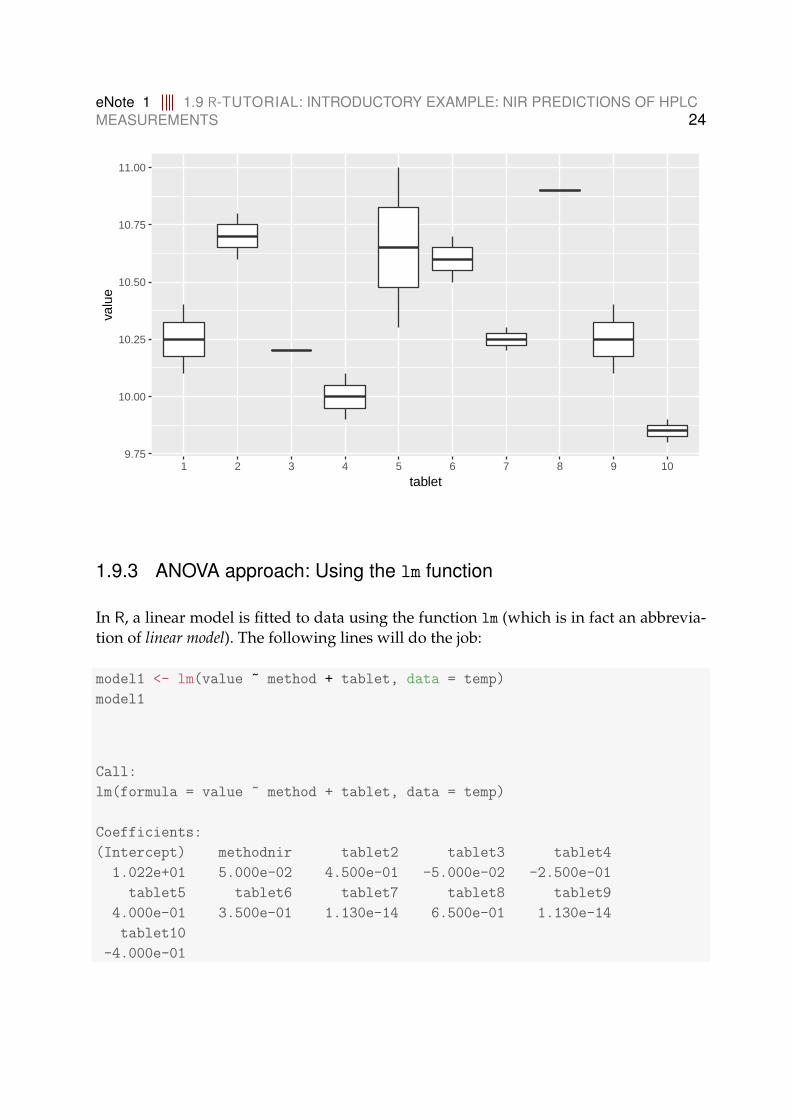
summary(model2)
Linear mixed model fit by REML [’lmerMod’]
Formula: value ~ method + (1 | tablet)
eNote 1 1.9 R-TUTORIAL: INTRODUCTORY EXAMPLE: NIR PREDICTIONS OF HPLCMEASUREMENTS 37
Data: temp
REML criterion at convergence: 14
Scaled residuals:
Min 1Q Median 3Q Max
-1.28851 -0.50128 -0.03985 0.52348 1.82403
Random effects:
Groups Name Variance Std.Dev.
tablet (Intercept) 0.08933 0.2989
Residual 0.04361 0.2088
Number of obs: 20, groups: tablet, 10
Fixed effects:
Estimate Std. Error t value
(Intercept) 10.34000 0.11530 89.678
methodnir 0.05000 0.09339 0.535
Correlation of Fixed Effects:
(Intr)
methodnir -0.405
anova(model2)
Analysis of Variance Table
Df Sum Sq Mean Sq F value
method 1 0.0125 0.0125 0.2866
As can be seen, the ANOVA table now focuses on the fixed effects, but it produces nop-value for the hypothesis test of no method effect. To get such a test directly, we canuse the Anova function from the car package:
Anova(model2, type = 3, test.statistic = "F")
Analysis of Deviance Table (Type III Wald F tests with Kenward-Roger df)
Response: value
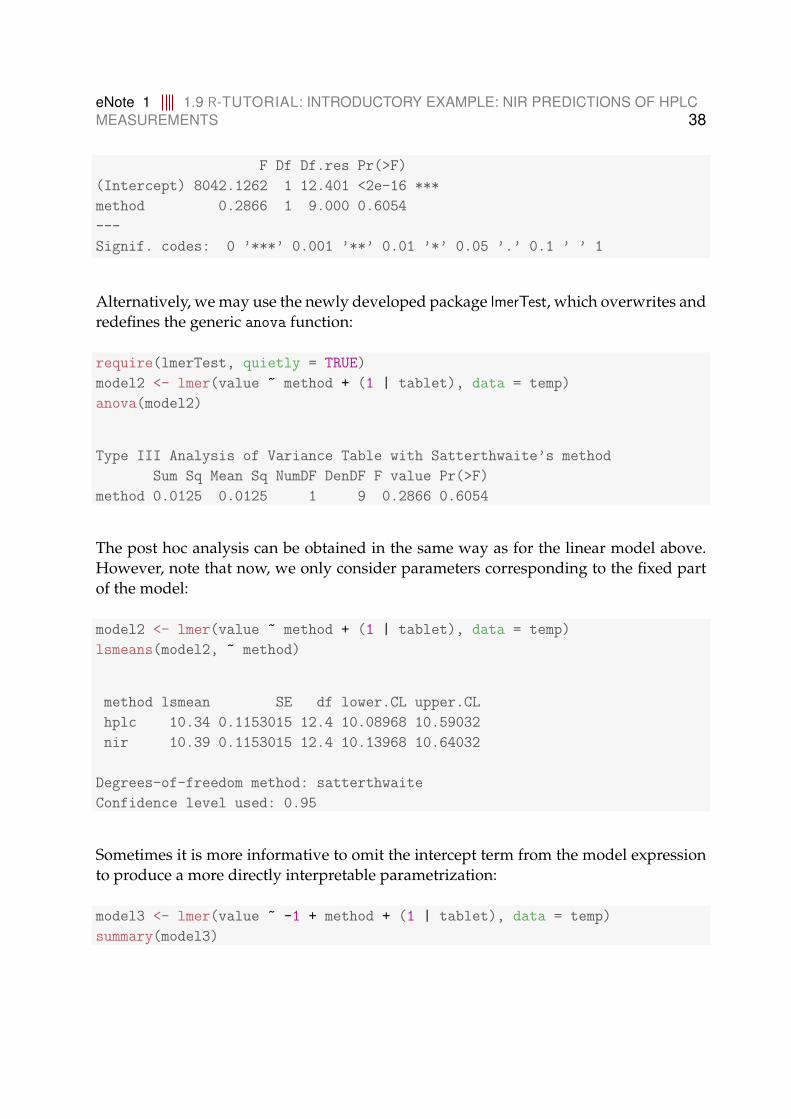
eNote 1 1.9 R-TUTORIAL: INTRODUCTORY EXAMPLE: NIR PREDICTIONS OF HPLCMEASUREMENTS 38
F Df Df.res Pr(>F)
(Intercept) 8042.1262 1 12.401 <2e-16 ***
method 0.2866 1 9.000 0.6054
---
Signif. codes: 0 ’***’ 0.001 ’**’ 0.01 ’*’ 0.05 ’.’ 0.1 ’ ’ 1
Alternatively, we may use the newly developed package lmerTest, which overwrites andredefines the generic anova function:
require(lmerTest, quietly = TRUE)
model2 <- lmer(value ~ method + (1 | tablet), data = temp)
anova(model2)
Type III Analysis of Variance Table with Satterthwaite’s method
Sum Sq Mean Sq NumDF DenDF F value Pr(>F)
method 0.0125 0.0125 1 9 0.2866 0.6054
The post hoc analysis can be obtained in the same way as for the linear model above.However, note that now, we only consider parameters corresponding to the fixed partof the model:
model2 <- lmer(value ~ method + (1 | tablet), data = temp)
lsmeans(model2, ~ method)
method lsmean SE df lower.CL upper.CL
hplc 10.34 0.1153015 12.4 10.08968 10.59032
nir 10.39 0.1153015 12.4 10.13968 10.64032
Degrees-of-freedom method: satterthwaite
Confidence level used: 0.95
Sometimes it is more informative to omit the intercept term from the model expressionto produce a more directly interpretable parametrization:
model3 <- lmer(value ~ -1 + method + (1 | tablet), data = temp)
summary(model3)

eNote 1 1.10 R-TUTORIAL: EXAMPLE WITH MISSING VALUES 39
Linear mixed model fit by REML. t-tests use Satterthwaite’s method [
lmerModLmerTest]
Formula: value ~ -1 + method + (1 | tablet)
Data: temp
REML criterion at convergence: 14
Scaled residuals:
Min 1Q Median 3Q Max
-1.28851 -0.50128 -0.03985 0.52348 1.82403
Random effects:
Groups Name Variance Std.Dev.
tablet (Intercept) 0.08933 0.2989
Residual 0.04361 0.2088
Number of obs: 20, groups: tablet, 10
Fixed effects:
Estimate Std. Error df t value Pr(>|t|)
methodhplc 10.3400 0.1153 12.4007 89.68 <2e-16 ***
methodnir 10.3900 0.1153 12.4007 90.11 <2e-16 ***
---
Signif. codes: 0 ’***’ 0.001 ’**’ 0.01 ’*’ 0.05 ’.’ 0.1 ’ ’ 1
Correlation of Fixed Effects:
mthdhp
methodnir 0.672
Note that the model is exactly the same, but now the lsmeans for the two methods aregiven directly.
1.10 R-TUTORIAL: Example with missing values
In this section, we go through the steps needed to do the calculations given in the in-troductory example with missing values The R-lines needed can be copied from above(changing the file names as necessary):

eNote 1 1.10 R-TUTORIAL: EXAMPLE WITH MISSING VALUES 40
hpnir2 <- read.table("hplcnir2.txt", header = TRUE, sep = ",")
temp2 <- data.frame(tablet = factor(rep(1:20, times = 2)),
method = rep(c("hplc", "nir"), each = 20),
y = c(hpnir2$hplc, hpnir2$nir))
temp2
tablet method y
1 1 hplc 10.4
2 2 hplc 10.6
3 3 hplc 10.2
4 4 hplc 10.1
5 5 hplc 10.3
6 6 hplc 10.7
7 7 hplc 10.3
8 8 hplc 10.9
9 9 hplc 10.1
10 10 hplc 9.8
11 11 hplc NA
12 12 hplc NA
13 13 hplc NA
14 14 hplc NA
15 15 hplc NA
16 16 hplc 10.3
17 17 hplc 9.6
18 18 hplc 10.0
19 19 hplc 10.2
20 20 hplc 9.9
21 1 nir 10.1
22 2 nir 10.8
23 3 nir 10.2
24 4 nir 9.9
25 5 nir 11.0
26 6 nir 10.5
27 7 nir 10.2
28 8 nir 10.9
29 9 nir 10.4
30 10 nir 9.9
31 11 nir 10.8
32 12 nir 9.8
33 13 nir 10.5

eNote 1 1.10 R-TUTORIAL: EXAMPLE WITH MISSING VALUES 41
34 14 nir 10.3
35 15 nir 9.7
36 16 nir NA
37 17 nir NA
38 18 nir NA
39 19 nir NA
40 20 nir NA
Note, again, that R uses NA for missing values.
1.10.1 Simple analysis using an ANOVA approach
The (modified) copies of the R-lines needed are then:
model1 <- lm(y ~ tablet + method, data = temp2)
anova(model1)
Analysis of Variance Table
Response: y
Df Sum Sq Mean Sq F value Pr(>F)
tablet 19 3.7230 0.195947 4.4931 0.01288 *
method 1 0.0125 0.012500 0.2866 0.60537
Residuals 9 0.3925 0.043611
---
Signif. codes: 0 ’***’ 0.001 ’**’ 0.01 ’*’ 0.05 ’.’ 0.1 ’ ’ 1
summary(model1)
Call:
lm(formula = y ~ tablet + method, data = temp2)
Residuals:
Min 1Q Median 3Q Max
-0.325 -0.025 0.000 0.025 0.325

eNote 1 1.10 R-TUTORIAL: EXAMPLE WITH MISSING VALUES 42
Coefficients:
Estimate Std. Error t value Pr(>|t|)
(Intercept) 1.022e+01 1.549e-01 66.021 2.12e-13 ***
tablet2 4.500e-01 2.088e-01 2.155 0.0596 .
tablet3 -5.000e-02 2.088e-01 -0.239 0.8161
tablet4 -2.500e-01 2.088e-01 -1.197 0.2618
tablet5 4.000e-01 2.088e-01 1.915 0.0877 .
tablet6 3.500e-01 2.088e-01 1.676 0.1281
tablet7 6.527e-15 2.088e-01 0.000 1.0000
tablet8 6.500e-01 2.088e-01 3.113 0.0125 *
tablet9 6.389e-15 2.088e-01 0.000 1.0000
tablet10 -4.000e-01 2.088e-01 -1.915 0.0877 .
tablet11 5.250e-01 2.600e-01 2.019 0.0742 .
tablet12 -4.750e-01 2.600e-01 -1.827 0.1010
tablet13 2.250e-01 2.600e-01 0.865 0.4093
tablet14 2.500e-02 2.600e-01 0.096 0.9255
tablet15 -5.750e-01 2.600e-01 -2.212 0.0543 .
tablet16 7.500e-02 2.600e-01 0.288 0.7795
tablet17 -6.250e-01 2.600e-01 -2.404 0.0396 *
tablet18 -2.250e-01 2.600e-01 -0.865 0.4093
tablet19 -2.500e-02 2.600e-01 -0.096 0.9255
tablet20 -3.250e-01 2.600e-01 -1.250 0.2428
methodnir 5.000e-02 9.339e-02 0.535 0.6054
---
Signif. codes: 0 ’***’ 0.001 ’**’ 0.01 ’*’ 0.05 ’.’ 0.1 ’ ’ 1
Residual standard error: 0.2088 on 9 degrees of freedom
(10 observations deleted due to missingness)
Multiple R-squared: 0.9049,Adjusted R-squared: 0.6936
F-statistic: 4.283 on 20 and 9 DF, p-value: 0.01492
Note that the order of the factors was changed compared to above – this is to obtain thesame Type I ANOVA table as in the example. Here, it depends on the order in which thefactors are specified in the model formula, as the data are not balanced. To get the posthoc lsmeans:
lsmeans(model1, ~ method)
method lsmean SE df lower.CL upper.CL

eNote 1 1.10 R-TUTORIAL: EXAMPLE WITH MISSING VALUES 43
hplc 10.2125 0.06177356 9 10.07276 10.35224
nir 10.2625 0.06177356 9 10.12276 10.40224
Results are averaged over the levels of: tablet
Confidence level used: 0.95
1.10.2 Analysis using a mixed model
Now use the missing values data set:
model2 <- lmer(y ~ method + (1 | tablet), data = temp2)
summary(model2)
Linear mixed model fit by REML. t-tests use Satterthwaite’s method [
lmerModLmerTest]
Formula: y ~ method + (1 | tablet)
Data: temp2
REML criterion at convergence: 24.7
Scaled residuals:
Min 1Q Median 3Q Max
-1.16659 -0.43803 0.00315 0.43635 1.84478
Random effects:
Groups Name Variance Std.Dev.
tablet (Intercept) 0.10192 0.3192
Residual 0.04347 0.2085
Number of obs: 30, groups: tablet, 20
Fixed effects:
Estimate Std. Error df t value Pr(>|t|)
(Intercept) 10.21175 0.09259 25.80968 110.288 <2e-16 ***
methodnir 0.07211 0.08697 11.69590 0.829 0.424
---
Signif. codes: 0 ’***’ 0.001 ’**’ 0.01 ’*’ 0.05 ’.’ 0.1 ’ ’ 1

eNote 1 1.11 EXERCISES 44
Correlation of Fixed Effects:
(Intr)
methodnir -0.470
and get the ANOVA table and lsmeans:
anova(model2)
Type III Analysis of Variance Table with Satterthwaite’s method
Sum Sq Mean Sq NumDF DenDF F value Pr(>F)
method 0.029887 0.029887 1 11.696 0.6875 0.4236
lsmeans(model2, ~ method)
method lsmean SE df lower.CL upper.CL
hplc 10.21175 0.09259176 25.81 10.02135 10.40214
nir 10.28386 0.09259176 25.81 10.09346 10.47425
Degrees-of-freedom method: satterthwaite
Confidence level used: 0.95
1.11 Exercises
Exercise 1 R start
1. Start R on your computer.
2. All data sets used in examples and exercises throughout the course are describedin eNote 13 (i.e. chapter 13 of the eBook) and are available for download from thecourse website.
3. Save the data file “hplcnir1.txt” on your computer, in the folder where you intendto save your analyses (i.e. the folder where you will put your R-files).
4. Import the data into R as described in this chapter.

eNote 1 1.11 EXERCISES 45
5. Try to reproduce the scatterplot of the NIR values versus the HPLC values givenin the main text by entering the relevant lines of R code from Section 1.8 into R.
Exercise 2 Sensory evaluation of cookies
Ten different chill or freezer storage treatments were tested on a type of cookies, andafter storage the cookies were evaluated by a sensory panel composed of 13 assessors.Each assessor tasted the cookies in a randomized order, and tasted each type twice. Inconnection with each test, the assessor gave a score for each of the following properties:colour, consistency, taste, and quality (a combined score). The score was an integer be-tween 0 and 10 with 10 being the best. The treatments are numbered 46, . . . , 55, and theassessors are numbered 1, . . . , 13. One assessor did not give any score for quality. Thedata set “cookies.txt” is available for download from the course website, and part of itis shown below:
assessor treatm colour cons taste quality
1 55 3 4 3 4
1 55 5 3 4 4
1 54 4 3 2 3
1 54 5 4 4 4
1 53 4 3 3 3
1 53 3 3 5 4
1 52 4 5 2 4
1 52 2 4 4 3
. . . . . . (There are 260 lines in the data set)
13 46 4 3 2 2
13 46 5 4 4 4
Focus on the quality response.
a) Think about which kind of plots would be suitable to explore the information inthe quality response, and try to make some of these.
b) Carry out a statistical analysis of the quality response with the aim of investigatingassessor and treatment differences (use ordinary analysis of variance techniques)and try to answer the following questions:

eNote 1 1.11 EXERCISES 46
1. Are there any assessor differences?
2. Are there any treatment differences?
3. Are possible treatment differences the same for all assessors?
(Did you make any plots which give an idea of the answer to these questions?)
The following lines of R-code may help as a start:
cookies <- read.table("cookies.txt", header = TRUE, sep = ",")
cookies$assessor <- factor(cookies$assessor)
cookies$treatm <- factor(cookies$treatm)
model1 <- lm(quality ~ assessor + treatm + assessor:treatm,
data = cookies)
anova(model1)
summary(model1)
c) Answer the same questions for the three other response variables: colour, cons andtaste.