Embed Size (px)
Citation preview

SALOME : The Open Source Integration Platform for Numerical Simulation
Copyright © 2001- 2010. All rights reserved.
Page 1 of 56
SA
LO
ME
P
la
tf
or
m
General Fuse Algorithm,
Partition Algorithm,
Boolean Operations Algorithm
Backgrounds

SALOME : The Open Source Integration Platform for Numerical Simulation
Copyright © 2001- 2010. All rights reserved.
Page 2 of 56
SA
LO
ME
P
la
tf
or
m
TABLE OF CONTENTS
1. INTRODUCTION.....................................................................................................................................................4
2. OVERVIEW ..............................................................................................................................................................4
3. ANALYSIS OF OPERATORS ................................................................................................................................5
4. TERMS AND DEFINITIONS..................................................................................................................................5
4.1. TOLERANCES .......................................................................................................................................................5 4.2. INTERFERENCES ...................................................................................................................................................5
4.2.1. Vertex/Vertex interference...........................................................................................................................5 4.2.2. Vertex/Edge interference.............................................................................................................................5 4.2.3. Vertex/Face interference .............................................................................................................................5 4.2.4. Edge/Edge interference ...............................................................................................................................5 4.2.5. Edge/Face interference ...............................................................................................................................5 4.2.6. Face/Face Interference ...............................................................................................................................5 4.2.7. Computation Order .....................................................................................................................................5 4.2.8. Results .........................................................................................................................................................5
4.3. PAVES ..................................................................................................................................................................5 4.4. PAVE BLOCKS ......................................................................................................................................................5 4.5. SHRUNK RANGE...................................................................................................................................................5 4.6. COMMON BLOCKS................................................................................................................................................5 4.7. CONNEXITY CHAINS ............................................................................................................................................5 4.8. SPLIT EDGES ........................................................................................................................................................5 4.9. SECTION EDGES ...................................................................................................................................................5
5. MAIN PARTS OF ALGORITHMS ........................................................................................................................5
5.1. DATA STRUCTURE ...............................................................................................................................................5 5.2. INTERSECTION PART ............................................................................................................................................5 5.3. BUILDING PART ...................................................................................................................................................5
6. GENERAL FUSE ALGORITHM ...........................................................................................................................5
6.1. ARGUMENTS ........................................................................................................................................................5 6.2. RESULTS ..............................................................................................................................................................5
6.2.1. Example 1....................................................................................................................................................5 6.2.2. Example 2....................................................................................................................................................5 6.2.3. Example 3....................................................................................................................................................5 6.2.4. Example 4....................................................................................................................................................5 6.2.5. Example 5....................................................................................................................................................5 6.2.6. Example 6....................................................................................................................................................5 6.2.7. Example 7....................................................................................................................................................5 6.2.8. Example 8....................................................................................................................................................5 6.2.9. Example 9....................................................................................................................................................5 6.2.10. Example 10..................................................................................................................................................5
7. PARTITION ALGORITHM ...................................................................................................................................5
7.1. ARGUMENTS ........................................................................................................................................................5 7.2. RESULTS ..............................................................................................................................................................5
7.2.1. Example 1....................................................................................................................................................5 7.2.2. Example 2....................................................................................................................................................5 7.2.3. Example 3....................................................................................................................................................5
8. BOOLEAN OPERATIONS ALGORITHM...........................................................................................................5
8.1. ARGUMENTS ........................................................................................................................................................5 8.2. RESULTS ..............................................................................................................................................................5
8.2.1. Example 1....................................................................................................................................................5 8.2.2. Example 2....................................................................................................................................................5 8.2.3. Example 3....................................................................................................................................................5 8.2.4. Example 4....................................................................................................................................................5
9. LIMITATIONS OF ALGORITHMS.......................... ............................................................................................5

SALOME : The Open Source Integration Platform for Numerical Simulation
Copyright © 2001- 2010. All rights reserved.
Page 3 of 56
SA
LO
ME
P
la
tf
or
m
9.1. ARGUMENTS ........................................................................................................................................................5 9.1.1. Common requirements ................................................................................................................................5 9.1.2. Pure self-interference..................................................................................................................................5 9.1.3. Self-interferences due to tolerances ............................................................................................................5 9.1.4. Parametric representation ..........................................................................................................................5 9.1.5. Stop-gaps.....................................................................................................................................................5
9.2. INTERSECTION PROBLEMS ....................................................................................................................................5 9.2.1. Pure intersections and common zones ........................................................................................................5 9.2.2. Tolerances ...................................................................................................................................................5

SALOME : The Open Source Integration Platform for Numerical Simulation
Copyright © 2001- 2010. All rights reserved.
Page 4 of 56
SA
LO
ME
P
la
tf
or
m
1. INTRODUCTION
This document describes the backgrounds of the following algorithms: General Fuse Algorithm, Partition
Algorithm, Boolean Operation Algorithm (hereafter Algorithms).
2. OVERVIEW
For the moment there are two algorithms that solve similar tasks:
• Boolean Operations Algorithm in Open CASCADE 6x (BOA).
BOA has been designed and developed in 2000. Since 2000 the algorithm is modified to fix the problems
upon requests (in general the modifications were bug fixes).
• Partition Algorithm for SALOME platform (PA).
PA has been designed and developed in 2005 and uses modern (at that time) algorithms of OCC as
auxiliary tools, for e.g. unbalanced binary tree of overlapped bounding boxes.
PA has the following features:
o PA is based on General Fuse Algorithm (GF).
o PA was developed taking into account the problems faced in BOA between 2000-2005 years.
o The architecture of PA is history-based and has been designed to support modern trends in topology
science.
o The architecture of PA is expandable, that allows to create a lot of specific algorithms upon requests.

SALOME : The Open Source Integration Platform for Numerical Simulation
Copyright © 2001- 2010. All rights reserved.
Page 5 of 56
SA
LO
ME
P
la
tf
or
m
3. ANALYSIS OF OPERATORS
• The General Fuse operator can be applied to arbitrary number of arguments (in terms of
TopoDS_Shape).
The operator can be represented as the following:
RGF=GF (S1, S2… Sn) (3.1.1)
where
RGF – result of the operation,
S1, S2 … Sn - Arguments of the operation,
n - Number of arguments (n>1)
• The Partition operator can be applied to arbitrary number of arguments (in terms of TopoDS_Shape).
The operator can be represented as the following:
RPA=PA (S1, S2… SnOB, [T1, T2… TnT]) (3.1.2)
where
RPA – result of the operation,
S1, S2 … SnOB - Arguments of the operation (Objects),
nOB - number of Objects (nOB>1)
T1, T2 … TnT - Arguments of the operation (Tools),
nT - number of Tools
It is evident that for nT=0
RPA=PA (S1, S2… SnOB)=RGF (3.1.3)
Thus, PA is particular case of GF.

SALOME : The Open Source Integration Platform for Numerical Simulation
Copyright © 2001- 2010. All rights reserved.
Page 6 of 56
SA
LO
ME
P
la
tf
or
m
• BOA provides the operations (Common, Fuse, Cut) between two arguments (in terms of
TopoDS_Shape).
The operator can be represented as the following:
RBOA=B j (S1, S2) (3.1.4)
where
RBOA – result of the operation
Bj – operation of type j (Common, Fuse, Cut),
S1, S2 - Arguments of the operation.
The result RBOA (3.1.4) can be obtained from RGF (3.1.1).
For e.g. for the two arguments S1, S2 (see the Figure 1) the result RGF will be
RGF=GF (S1, S2) = S p1+S p2+Sp12 (3.1.5)
Figure 1
S1
S2
Sp1
Sp2
Sp12

SALOME : The Open Source Integration Platform for Numerical Simulation
Copyright © 2001- 2010. All rights reserved.
Page 7 of 56
SA
LO
ME
P
la
tf
or
m
On the other hand
Bcommon (S1, S2) = Sp12
Bcut12 (S1, S2) = Sp1
Bcut21 (S1, S2) = Sp2
Bfuse (S1, S2) = S p1+S p2+Sp12 = RGF
(3.1.6)
RGF=GF (S1, S2) = Bfuse = Bcommon + Bcut12+ Bcut21 (3.1.7)
The fact that the RGF contains the components of RB (3.1.7) allows to consider that GF is the general
case of BOA. Thus it is possible to implement BOA, PA as subclasses of GF using C++ inheritance
mechanism.

SALOME : The Open Source Integration Platform for Numerical Simulation
Copyright © 2001- 2010. All rights reserved.
Page 8 of 56
SA
LO
ME
P
la
tf
or
m
4. TERMS AND DEFINITIONS
The chapter contains the background, terms, definitions that are necessary to understand how the
algorithms work.
4.1. TOLERANCES
Each shape that has boundary representation in the Open CASCADE contains its own internal value of
geometrical tolerance.
The meaning of the tolerance is different for different shapes (Table 1).
Table 1
No Picture Description
1
Vertex
Value of the tolerance for a vertex V is the value
of radii of a imaginary circumscribed sphere
around the 3-D point of the vertex V
2
Edge
Value of the tolerance for an edge E is the value
of radii of a imaginary circumscribed pipe around
the 3-D curve of the edge E
3
Face
Value of the tolerance for a face F is the value of
thickness of a imaginary offset surfaces to
underlying surface of the face F
Tol
V
Tol E
2Tol
F

SALOME : The Open Source Integration Platform for Numerical Simulation
Copyright © 2001- 2010. All rights reserved.
Page 9 of 56
SA
LO
ME
P
la
tf
or
m
Tolerance is a way of stating how much precision is needed or conversely, how much error can be to accept
the shape.
The tolerances in Open CASCADE are absolute values (in some units: mm, in, etc). Absolute tolerance
defines the maximum permissible distance apart that two shapes (or sub-shapes) are permitted to be and
still be considered to be “close enough”, i.e. that these two shapes will be capable of being joined.
There are the following rules for the values of tolerances:
• For any edge E with vertices Vi:
Tol (E) ≤ max (Tol (V i)), i=1, 2…NbV (4.1.1)
where NbV – Number of vertices of the edge E.
• For any edge face F with edges Ei:
Tol (F) ≤ max (Tol (E i)), i=1, 2…NbE (4.1.2)
where NbE - Number of edges of the face F.

SALOME : The Open Source Integration Platform for Numerical Simulation
Copyright © 2001- 2010. All rights reserved.
Page 10 of 56
SA
LO
ME
P
la
tf
or
m
4.2. INTERFERENCES
The shapes interferes between each other in terms of theirs tolerances.
Shapes are interfered when there is a part of 3D space where the distance between the underlying geometry
of shapes is less or equal to the sum of tolerances of the shapes.
For the three types of shapes (vertex, edge, face) there are six types of interferences.
4.2.1. Vertex/Vertex interference
A vertex Vi and a vertex Vj have Vertex/Vertex interference when VI and Vj have the distance between
corresponding 3D points that is less then sum of the tolerances Tol(V i) and Tol(V j) of the vertices (Figure 2).
Figure 2
Result:
New vertex Vn with 3D point Pn and tolerance value Tol(Vn) that can be computed by the formulas:
Pnew = 0.5•(Pi + Pj)
Tol (V n) = max (Tol(V i), Tol(V j)) + 0.5•D
where
D=distance (P i, Pj)
Tol (Vi) Tol (Vj)
Vj Vi
T s
D
Tol(Vn)
Vn
Pn

SALOME : The Open Source Integration Platform for Numerical Simulation
Copyright © 2001- 2010. All rights reserved.
Page 11 of 56
SA
LO
ME
P
la
tf
or
m
4.2.2. Vertex/Edge interference
A vertex Vi and an edge Ej have Vertex/Edge interference when for the vertex Vi and the edge Ej the
distance D between 3D point of the vertex and its projection on the 3D curve of the edge Ej is less or equal
than sum of tolerances of the vertex Tol(V i) and the edge Tol(E j) (Figure 3).
Figure 3
Result:
• Vertex Vi with the corresponding tolerance value.
Tol(V i) = max (Tol(V i), Tol(E j)) + 0.5•D
where
D=distance (P i, PPi)
• Parameter ti of the projected point PPi on the 3D curve Cj of the edge Ej.
Ej
Vi
Tol(E j)
Tol(V i)
Vi
Cj
Tol(V i)
t i PPi
Pi

SALOME : The Open Source Integration Platform for Numerical Simulation
Copyright © 2001- 2010. All rights reserved.
Page 12 of 56
SA
LO
ME
P
la
tf
or
m
4.2.3. Vertex/Face interference
A vertex Vi and a face Fj have Vertex/Face interference when for the vertex Vi and the face Fj the distance D
between 3D point of the vertex and its projection on the surface of the face is less or equal than sum of
tolerances of the vertex Tol(V i) and the face Tol(F j) (Figure 4).
Figure 4
Result:
• Vertex Vi with the corresponding tolerance value.
Tol(V i) = max (Tol(V i), Tol(E j)) + 0.5•D
where
D=distance (P i, PPi)
• Parameters ui, vi of the projected point PPi on the surface Sj of the face Fj.
Tol(V i)
Fj
Vi Pi
PPi
2•Tol(F j) •
Tol(V i)
Fj
Vi Pi
PPi
u
vvi
ui
Fj

SALOME : The Open Source Integration Platform for Numerical Simulation
Copyright © 2001- 2010. All rights reserved.
Page 13 of 56
SA
LO
ME
P
la
tf
or
m
4.2.4. Edge/Edge interference
An edge Ei and an edge Ej have Edge/Edge interference when for two of edges Ei and Ej (with
corresponding 3D curves Ci, Cj) there is (are) some place(s) where the distance between the curves is less
than (or equals to) sum of tolerances of the edges.
Case 1: Two edges have common part(s) of 3D curves in terms of tolerance (Figure 5).
Figure 5
Result:
• Parametric range [ti1, ti2 ] for the 3D curve Ci of the edge Ei.
• Parametric range [tj1, tj2 ] for the 3D curve Cj of the edge Ej.
Ej
Tol(E j) Tol(E i)
Ei
Ej Ei
t j2 t j1
Cj

SALOME : The Open Source Integration Platform for Numerical Simulation
Copyright © 2001- 2010. All rights reserved.
Page 14 of 56
SA
LO
ME
P
la
tf
or
m
Case 2: Two edges have common point(s) in terms of tolerance (Figure 6).
Figure 6
Result:
• New vertex (-ices) Vn with 3D point Pn and tolerance value Tol(Vn) that are calculated by the formulas:
Pn = 0.5•(Pi + Pj)
Tol(V n) = max (Tol(E i), Tol(E j)) + 0.5•D
where
D=distance (P i, Pj)
Pi, Pj – the nearest 3D points for the curves Ci, Cj
• Parametr ti of Pi for the 3D curve Ci.
• Parametr tj of Pj for the 3D curve Cj.
Ej
Tol(E j)
Ei
Tol(E i)
Ej
Ei
t j
Cj
Vn Tol(Vn)
Ci P
t i

SALOME : The Open Source Integration Platform for Numerical Simulation
Copyright © 2001- 2010. All rights reserved.
Page 15 of 56
SA
LO
ME
P
la
tf
or
m
4.2.5. Edge/Face interference
An edge Ei and a face Fj have Edge/Face interference when for the edge Ei and the face Fj (with
corresponding 3D curve Ci, and surface Sj) there is (are) some place(s) in 3D space where the distance
between the Ci and the surface Sj is less than (or equal to) sum of tolerances of the edge Ei and the face Fj.
Case 1: Edge Ei and Face Fj have common part(s) in terms of tolerance (Figure 7).
Figure 7
Result:
• Parametric range [ti1, ti2 ] for the 3D curve Ci of the edge Ei.
Tol(E i)
Fj
2•Tol(F j)
Ei
Fj Ei
Ci
t i2
t i1

SALOME : The Open Source Integration Platform for Numerical Simulation
Copyright © 2001- 2010. All rights reserved.
Page 16 of 56
SA
LO
ME
P
la
tf
or
m
Case 2: Edge Ei and Face Fj have common point(s) in terms of tolerance (Figure 8).
Figure 8
Result:
• New vertex (-ices) Vn with 3D point Pn and tolerance value Tol(Vn) that are calculated by the formulas:
Pn = 0.5•(Pi + Pj)
Tol (V n) = max (Tol (E i), Tol (F j)) + 0.5•D
where
D=distance (P i, Pj)
Pi, Pj – the nearest 3D points for the curve Ci and surface Sj
• Parameter ti of Pi for the 3D curve Ci.
• Parameters ui, vi of the projected point PPi on the surface Sj of the face Fj.
Tol(E i)
Fj
2•Tol(F j)
Ei
Fj
Ei
Tol(Vn)
Vn
Ci
t i

SALOME : The Open Source Integration Platform for Numerical Simulation
Copyright © 2001- 2010. All rights reserved.
Page 17 of 56
SA
LO
ME
P
la
tf
or
m
4.2.6. Face/Face Interference
A face Fi and a face Fj have Face/Face interference when for the face Fi and the face Fj (with corresponding
surfaces Si, Sj) there are some place(s) in 3D space where the distance between the surfaces is less than
(or equal to) sum of tolerances of the faces.
Case 1: Face Fi and face Fj have common curve(s) Cijk (k=0, 1, 2…kn) in terms of tolerance (Figure 9).
Figure 9
Result:
• Intersection curves Cijk (k=0, 1, 2…kn, kn - number of intersection curves) with correspondent values of
tolerances Tol(C ijk ).
Tol(C ijk ) Fi
2•Tol(F j)
2•Tol(F i)
Fj Cijk

SALOME : The Open Source Integration Platform for Numerical Simulation
Copyright © 2001- 2010. All rights reserved.
Page 18 of 56
SA
LO
ME
P
la
tf
or
m
Case 2: Face Fi and face Fj have common point(s) in terms of tolerance (Figure 10).
Figure 10
Result:
• New vertices Vijm (m=0, 1, 2, mn, - number of intersection points).
• New vertex (-ices) Vijm with 3D point Pn and tolerance value Tol(Vn) that are calculated by the formulas:
Pn = 0.5•(Pi + Pj)
Tol(V ijm ) = max (Tol(F i), Tol(F j)) + 0.5•D
where
D=distance (P i, Pj)
Pi, Pj – the nearest 3D points for the surface Si and surface Sj.
• Parameters ui , vi of the projected point PPj on the surface Sj of the face Fj
• Parameters ui , vi of the projected point PPi on the surface Si of the face Fi
4.2.7. Computation Order
The interferences between shapes are computed on the basis of increasing of the dimension value of the
shape in the following order: Vertex/Vertex, Vertex/Edge, Edge/Edge, Vertex/Face, Edge/Face,
Face/Face . The reason is to avoid the computation of redundant interferences between upper shapes Si, Sj
when there are interferences between lower sub-shapes Sik, Sjm.
Tol(V ijm)
Fi
2•Tol(F j)
2•Tol(F i)
Fj
Vijm

SALOME : The Open Source Integration Platform for Numerical Simulation
Copyright © 2001- 2010. All rights reserved.
Page 19 of 56
SA
LO
ME
P
la
tf
or
m
4.2.8. Results
• The result of the interference is a shape that can be either interfered shape itself (or its part) or a new
shape.
• The result of the interference is a shape with the dimension value that is less or equal to the minimal
dimension value of interfered shapes. For e.g. the result of Vertex/Edge interference is a vertex, but not
an edge.
• The result of the interference splits source shapes on parts each time as it can do that.
4.3. PAVES
The result of interferences of the type Vertex/Edge, Edge/Edge, Edge/Face in a number of cases is a vertex
(new or old) lying on the edge.
The result of interferences of the type Face/Face in a number of cases is intersection curves. These curves
go through the vertices lying on the faces.
The position of the vertex Vi on the curve C is determined by a value of a parameter t i of the 3D point of the
vertex on the curve.
A Pave PVi on a curve C is a structure containing the vertex Vi and correspondent value of the parameter t i
of the of the 3D point of the vertex on the curve. The curve C can be 3D or 2D curve. (Figure 11)
Figure 11
Two paves PV1, PV2 on the one curve C can be compared using the parameter value. PV1>PV2 if t1 > t2.
The usage of paves allows making the difference between the one vertex V shared between arbitrary
number of edges E1, E2, …Ei
The usage of paves allows to bind the vertex to the curve (or any structure that contains a curve: edge,
intersection curve).
PVb
E
C
PVe
PVi t i
te
tb=0
Ve Vb
Vi

SALOME : The Open Source Integration Platform for Numerical Simulation
Copyright © 2001- 2010. All rights reserved.
Page 20 of 56
SA
LO
ME
P
la
tf
or
m
4.4. PAVE BLOCKS
A set of paves PVi (i=1, 2...nPV, nPV- number of paves) of the curve C can be sorted in increasing order
using the value of parameter t on the curve C.
A pave block PBi is a part of the object (edge, intersection curve) between neighboring paves. (Figure 12)
Figure 12
Any finite source edge E has the one bounding pave block that contains two paves PVb, PVe. The pave PVb
corresponds to the vertex Vb with minimal parameter tb on the curve of the edge. The pave PVe corresponds
to the vertex Ve with maximal parameter te on the curve of the edge.
PVb
E
C
PVe
PVi
tb=0
Ve Vb
Vi
PVh PVj th
t i
t j
te
Vh
Vj
PB i

SALOME : The Open Source Integration Platform for Numerical Simulation
Copyright © 2001- 2010. All rights reserved.
Page 21 of 56
SA
LO
ME
P
la
tf
or
m
4.5. SHRUNK RANGE
A pave block PV (Figure 13) of a curve C is bounded by vertices V1, V2 with the values of tolerances Tol(V1),
Tol(V2).
The curve C has a value of tolerance Tol(C) . In case of edge the value of tolerance is tolerance of the edge.
In case of intersection curve the value of tolerance is obtained from an intersection algorithm.
Figure 13
The theoretical parametric range of the pave block is [t 1C, t2C].
The positions of the vertices V1, V2 of the pave block can be different and are determined by the following
conditions:
Distance (P 1, P1c) ≤ Tol(V 1)+Tol(C)
Distance (P 2, P2c) ≤ Tol(V 2)+Tol(C)
The Figure 13 shows that each tolerance sphere of a vertex can reduce the parametric range of the pave
block to [t 1S, t2S]. The range [t 1S, t2S] is the shrunk range of the pave block. At limiting state t1S=t1C, t2S=t2C.
The shrunk range of the pave block is the part of 3D curve that can interfere with other shapes.
V1
V2
C (t)
Tol (V2) Tol (V1) Tol (C)
t1C
t2C t2S t1S
P1
P2
P2C
P1C

SALOME : The Open Source Integration Platform for Numerical Simulation
Copyright © 2001- 2010. All rights reserved.
Page 22 of 56
SA
LO
ME
P
la
tf
or
m
4.6. COMMON BLOCKS
The interferences of the type Edge/Edge, Edge/Face can produce results as common parts. In case of
Edge/Edge interference the common parts are pave blocks having different edges as a base. (Figure 14)
Figure 14
If the pave blocks PV1, PV2…PVNbPV (NbPV – number of the pave blocks) have the same bounding vertices
and geometrically coincide, the pave blocks form common block CB.
In case of Edge/Face interference the common parts are pave block lying on a face(s) (Figure 15).
Figure 15
If the pave blocks PVi geometrically coincide with a face Fj, the pave block form common block CB.
In general case a common block CB contains:
• Pave blocks PVi (i=2, 3… NbPV)
• A set of faces Fj (j=0,1..NbF, NbF – number of faces).
V11 PB
F2
F3 E
CB
Vi
Vj
E1
E2
V11 V12
V21 V22
CB
PB2
PB1

SALOME : The Open Source Integration Platform for Numerical Simulation
Copyright © 2001- 2010. All rights reserved.
Page 23 of 56
SA
LO
ME
P
la
tf
or
m
4.7. CONNEXITY CHAINS
The interfering shapes can produce connexity chains.
The term connexity chains can be explained by the following examples
• Interfering vertices. (Figure 16)
Figure 16
The pairs of interfered vertices are: (nV11, nV12), (nV11, nV13), (nV12, nV13), (nV13, nV15), (nV13, nV14), (nV14,
nV15), (nV21, nV22), (nV21, nV23), (nV22, nV23)
The pairs produce the two connexity chains: (nV11, nV12, nV13, nV14, nV15), (nV21, nV22, nV23).
Each connexity chain is used to create new vertex: VN1, VN2.
• Interfering edges (Figure 17)
Figure 17
The pairs of coincided pave blocks are: (PB11, PB12), (PB11, PB13), (PB12, PB13), (PB21, PB22), (PB21, PB23),
(PB22, PB23)
PB11
PB12
PB13
PB21
PB22
PB22
Chain 1 Chain 2
V11
V12
V13
V14
V15
V21
V22
V23
Chain 1 Chain 2
VN1 VN2

SALOME : The Open Source Integration Platform for Numerical Simulation
Copyright © 2001- 2010. All rights reserved.
Page 24 of 56
SA
LO
ME
P
la
tf
or
m
The pairs produce the two connexity chains: (PB11, PB12, PB13), (PB21, PB22, PB23).
• Interfering faces (Figure 18)
Figure 18
The pairs of same domain faces are: (F11, F21), (F22, F31), (F41, F51) , (F41, F6) , (F51, F6)
The pairs produce the three connexity chains: (F11, F21), (F22, F31), (F41, F51, F6)
A connexity chain contains shapes that are Same Domain Shapes (same domain vertices, same domain
edges, same domain faces).
4.8. SPLIT EDGES
The set of pave blocks PB1, PB2… PBnPB (nPB – number of pave blocks) for the edge E is used to build split
edges Spi (i=1, 2…nPB).
4.9. SECTION EDGES
The set of pave blocks PB1, PB2… PBnPB (nPB – number of pave blocks) for the intercestion curve C is used
to build section edges Sci (i=1, 2…nPB).
F2
Chain 1 Chain 2
F1 F3
F4
F5
F11 F21 F22
F31 F6 F51
F41

SALOME : The Open Source Integration Platform for Numerical Simulation
Copyright © 2001- 2010. All rights reserved.
Page 25 of 56
SA
LO
ME
P
la
tf
or
m
5. MAIN PARTS OF ALGORITHMS
The Algorithms (GF, PA, BOA) consist of three parts:
5.1. DATA STRUCTURE
Data Structure (DS) is used tob
• Store information for data and intermediate results
• Provide the access to the information
• Provide the links between chunks of information
The contents of the information are:
• Arguments
• New shapes
• Interferences
• Pave Blocks
• Common Blocks
5.2. INTERSECTION PART
Intersection Part (IP) is used to
• Initialize DS
• Compute interferences between the arguments (and their sub-shapes)
• Compute same domain vertices, edges
• Build split edges
• Build section edges
• Build p-Curves
• Store all obtained information in DS
IP uses DS as input data.
5.3. BUILDING PART
Building Part (BP) is used to
• Build sub-shapes of the result of the operation
• Build the result of the operation

SALOME : The Open Source Integration Platform for Numerical Simulation
Copyright © 2001- 2010. All rights reserved.
Page 26 of 56
SA
LO
ME
P
la
tf
or
m
• Provide history information (in terms of BRepBuilderAPI_MakeShape::Generated(), ::Modified(),
:IsDeleted())
BP uses DS as input data.
6. GENERAL FUSE ALGORITHM
6.1. ARGUMENTS
• The arguments are shapes (in terms of TopoDS_Shape).
• Number of arguments is non-limited
• Each argument is valid shape (in terms of BRepCheck_Analyzer);
• Each argument can be one of the following types (see theTable 2)
Table 2
No Type Index of Type
1 COMPOUND 0
2 COMPSOLID 1
3 SOLID 2
4 SHELL 3
5 FACE 4
6 WIRE 5
7 EDGE 6
8 VERTEX 7
• The argument of type 0 (COMPOUND) can include any number of shapes of any type (0, 1…7).
• The argument should not be self-interfered, i.e. all sub-shapes of the argument that have geometrical
coincidence through any topological entities (vertices, edges, faces) must share these entities.

SALOME : The Open Source Integration Platform for Numerical Simulation
Copyright © 2001- 2010. All rights reserved.
Page 27 of 56
SA
LO
ME
P
la
tf
or
m
6.2. RESULTS
• During the operation the argument Si can be splitted on parts (Si1, Si2… Si1NbSp, NbSp - number of the
parts). The set (Si1, Si2… Si1NbSp) is image of the argument Si.
• The result of GF operation is a compound. Each sub-shape of the compound (resulting shape)
corresponds to the concrete argument shape S1, S2…Sn and has shared sub-shapes in accordance with
interferences between the argument and the others.
• For the arguments of the type EDGE, FACE, SOLID the result contains split parts of the argument
• For the arguments of the type WIRE, SHELL, COMPSOLID, COMPOUND the result contains the image
of the shape with the corresponding type (i.e. WIRE, SHELL, COMPSOLID, and COMPOUND.
The types of resulting shapes depend on the type of the corresponding argument (Table 3).
Table 3
No Type of argument Type of resulting
shape
Comments
1 COMPOUND COMPOUND The resulting COMPOUND is built from
• Images of sub-shapes of type COMPOUND
COMPSOLID, SHELL, WIRE, VERTEX
• Sets of splitted sub-shapes of type SOLID, FACE,
EDGE
2 COMPSOLID COMPSOLID The resulting COMPSOLID is built from split SOLID-s
3 SOLID Set of split SOLID-s
4 SHELL SHELL The resulting SHELL is built from split FACE-s
5 FACE Set of split FACE-s
6 WIRE WIRE The resulting WIRE is built from split
EDGE-s
7 EDGE Set of split EDGE-s
8 VERTEX VERTEX
The following set of examples is to clarify the definition above.

SALOME : The Open Source Integration Platform for Numerical Simulation
Copyright © 2001- 2010. All rights reserved.
Page 28 of 56
SA
LO
ME
P
la
tf
or
m
6.2.1. Example 1
The arguments are three edges E1, E2, E3 (Figure 19), that intersect in one 3D point.
Figure 19
The result of GF operation is compound.
The compound contains 6 new edges E11, E12, E21, E22, E31, and E32. These edges have one shared vertex
Vn1.
In this case:
• the argument edge E1 has resulting split edges E11, E12 (image of E1),
• the argument edge E2 has resulting split edges E21, E22 (image of E2),
• the argument edge E3 has resulting split edges E31, E32. (image of E3).
E1
E2 E3
Vn1
E31
E11
E21
E12
E22 E32

SALOME : The Open Source Integration Platform for Numerical Simulation
Copyright © 2001- 2010. All rights reserved.
Page 29 of 56
SA
LO
ME
P
la
tf
or
m
6.2.2. Example 2
The arguments are two wires W1 (Ew11, Ew12, Ew13), W2 (Ew21, Ew22, Ew23) and the edge E1 (Figure 20).
Figure 20
The result of GF operation is compound.
The compound consist of 2 wires Wn1 (Ew11, En1, En2, En3, Ew13), Wn2 (Ew21, En2, En3, En4, Ew23) and
edges E11, E12.
In this case
• the argument W1 has image Wn1,
• the argument W2 has image Wn2,
• the argument edge E1 has split edges E11, E22. (image of E1)
The edges En1, En2, En3, En4 and the vertex Vn1 are new shapes created during the operation so as the
edge Ew12 has split edges En1, En2, En3, the edge Ew22 has split edges En2, En3, En4.
E1 W1
W2
Ew21
Ew22
Ew23
Ew11
Ew12
Ew13
E11 Wn1
W2
Ew11 Ew13
Ew21 Ew23
E12
En1 En2 En3 En4
Vn1

SALOME : The Open Source Integration Platform for Numerical Simulation
Copyright © 2001- 2010. All rights reserved.
Page 30 of 56
SA
LO
ME
P
la
tf
or
m
6.2.3. Example 3
The arguments are the edge E1 and the face F2 (Figure 21).
Figure 21
The result of GF operation is compound.
The compound consists of 3 shapes:
• Split parts of the edge E11, E12 (image of E1)
• New face F21 with internal edge E12. (image of F2)
6.2.4. Example 4
The arguments are the edge E1 and the face F2 (Figure 22).
Figure 22
The result of GF operation is compound. The compound consists of 5 shapes:
• Split parts of the edge E11, E12 , E13 (image of E1),
• Split parts of the face F21, F22 (image of F2)
E1
F2
F21
E11 E12
E12
E1
F2
F21
F22
E12
E12
E11 E13

SALOME : The Open Source Integration Platform for Numerical Simulation
Copyright © 2001- 2010. All rights reserved.
Page 31 of 56
SA
LO
ME
P
la
tf
or
m
6.2.5. Example 5
The arguments are the edge E1 and the shell Sh2 that consists of 2 faces F21, F22 (Figure 23).
Figure 23
The result of GF operation is compound. The compound consists of 5 shapes:
• Split parts of the edge E11, E12 , E13, E14 (image of E1)
• Image shell Sh21 (that contains split parts of the faces F211, F212, F221, F222)
6.2.6. Example 6
The arguments are the wire W1 (E1, E2, E3, E4) and the shell Sh2 (F21, F22) (Figure 24).
Figure 24
The result of GF operation is compound. The compound consists of 2 shapes:
• Image wire W11 that consist of split parts of the edges of W1: E11, E12 , E13, E14
• Image shell Sh21 that contains split parts of the faces F211, F212, , F213, F221, F222, F223
F21
F22
E1 E11
E14
F212
F222
F211
F221
E13
E12
F21
F22 W1
F212
F222
F211
F221
F223
F213
W11
Sh2
E11 E12
E13 E14
Sh21
E1 E2
E3 E4

SALOME : The Open Source Integration Platform for Numerical Simulation
Copyright © 2001- 2010. All rights reserved.
Page 32 of 56
SA
LO
ME
P
la
tf
or
m
6.2.7. Example 7
The arguments are 3 faces F1, F2, F3 (Figure 25).
Figure 25
The result of GF operation is compound. The compound consists of 7 shapes:
• Split parts of the faces Fn1, Fn2, Fn3, Fn4, Fn5, Fn6, Fn7
6.2.8. Example 8
The arguments are the shell Sh1 (F11, F12, F13) and the face F2 (Figure 26).
Figure 26
The result of GFoperation is compound. The compound consists of 4 shapes:
• Image shell Sh11 that consist of split parts of the faces of Sh1: Fn1, Fn2, Fn3, Fn4, Fn5, Fn6
• Split parts of the face F2: Fn3, Fn6, Fn7
F1
F3
F2
Fn1
Fn2
Fn3
Fn4
Fn5
Fn6
Fn7
Fn1
Fn2
Fn3
Fn4
Fn5
Fn6
Fn7
F2
Sh1
F11
F12 F13

SALOME : The Open Source Integration Platform for Numerical Simulation
Copyright © 2001- 2010. All rights reserved.
Page 33 of 56
SA
LO
ME
P
la
tf
or
m
6.2.9. Example 9
The arguments are the shell Sh1 (F11, F12…F16) and the solid So2 (Figure 27).
Figure 27
The result of GF operation is compound.
The compound consists of 2 shapes (Figure 28)
• Image shell Sh11 that consist of split parts of the faces of Sh1: Fn1, Fn2….Fn8.
• Solid So21 with internal shell. (image of So2)
Figure 28
So2
Sh1
Fn1
Fn2 Fn2
Fn4 Fn4
Fn3 Fn3
Fn1
Fn5
Fn6
Fn7 Fn8
So21
Sh11

SALOME : The Open Source Integration Platform for Numerical Simulation
Copyright © 2001- 2010. All rights reserved.
Page 34 of 56
SA
LO
ME
P
la
tf
or
m
6.2.10. Example 10
The arguments are the compound Cm1 (of 2 solids So11, So12) and the solid So2 (Figure 29).
Figure 29
The result of GF operation is compound. The compound consists of 4 shapes (Figure 30)
• Image compound Cm11 that consists of split parts of the solids of So11, So12 (Sn1, Sn2, Sn3, Sn4).
• Split parts of the solid So2 (Sn2, Sn3, Sn5).
Figure 30
Fn7
So11
So2
So12
Sn1
Sn2
Sn3
Sn4
Sn2
Sn5 Sn3
Sn1
Sn2
Sn3
Sn4
Sn2
Sn5
Sn3

SALOME : The Open Source Integration Platform for Numerical Simulation
Copyright © 2001- 2010. All rights reserved.
Page 35 of 56
SA
LO
ME
P
la
tf
or
m
7. PARTITION ALGORITHM
7.1. ARGUMENTS
The arguments of the algorithm are shapes (in terms of TopoDS_Shape). The main requirements for the
arguments are described in 6.1
The arguments in PA are separated in two groups:
• Shapes
• Tools
7.2. RESULTS
The main difference between GF and PA algorithms is in the rules of building the result.
• For arguments of Shapes group the rules are the same as it has been described in 6.2.
• For the arguments of Tools group there is the following rule: The result should not contain any shape St i
from Tools group or image of the shape St i (St i1, St i2...StiNbt Nbt - number of Tools) from Tools group if
these shapes are not included in images of Shapes group.
• The result will contain shapes that have complexity (in terms of TopAbs_ShapeEnum) that is less or
equal to given Limit. The values of Limit can have any value. In case when Limit =TopAbs_SHAPE the
result will contain shapes with complexity that corresponds to the complexity of the arguments.

SALOME : The Open Source Integration Platform for Numerical Simulation
Copyright © 2001- 2010. All rights reserved.
Page 36 of 56
SA
LO
ME
P
la
tf
or
m
7.2.1. Example 1
The arguments are
• Shapes: edges E1, E2
• Tools: edge E3 (Figure 31)
• Limit : TopAbs_SHAPE
Figure 31
The result of PA operation is compound.
The compound contains 4 new edges E11, E12, E21, E22. These edges have one shared vertex Vn1.
In this case:
• the argument edge E1 has resulting split edges E11, E12 (image of E1),
• the argument edge E2 has resulting split edges E21, E22 (image of E2)
E1
E2 E3
Vn1
E31
E11
E21
E12
E22

SALOME : The Open Source Integration Platform for Numerical Simulation
Copyright © 2001- 2010. All rights reserved.
Page 37 of 56
SA
LO
ME
P
la
tf
or
m
7.2.2. Example 2
The arguments are
• Shapes: wire W1 (Ew11, Ew12, Ew13) and the edge E1
• Tools: wire W2 (Ew21, Ew22, Ew23) (Figure 32).
• Limit : TopAbs_SHAPE
Figure 32
The result of PA operation is compound.
The compound consist of wire Wn1 (Ew11, En1, En2, En3, Ew13), and edges E11, E12.
In this case
• the argument W1 has image Wn1
• the argument edge E1 has split edges E11, E22. (image of E1)
The edges En1, En2, En3, En4 and the vertex Vn1 are new shapes created during the operation so as the
edge Ew12 has split edges En1, En2, En3, the edge Ew22 has split edges En2, En3, En4.
E1 W1
W2
Ew21
Ew22
Ew23
Ew11
Ew12
Ew13 E11 Wn1
Ew11 Ew13
E12
En1 En2 En3
Vn1

SALOME : The Open Source Integration Platform for Numerical Simulation
Copyright © 2001- 2010. All rights reserved.
Page 38 of 56
SA
LO
ME
P
la
tf
or
m
7.2.3. Example 3
The arguments are
• Shapes: the face F2
• Tools: the edge E1 (Figure 33).
• Limit : TopAbs_FACE
Figure 33
The result of PA operation is compound.
The compound consists of 3 shapes:
• New face F21 with internal edge E12. (image of F2)
E1
F2 F21
E12

SALOME : The Open Source Integration Platform for Numerical Simulation
Copyright © 2001- 2010. All rights reserved.
Page 39 of 56
SA
LO
ME
P
la
tf
or
m
8. BOOLEAN OPERATIONS ALGORITHM
8.1. ARGUMENTS
• The arguments are shapes (in terms of TopoDS_Shape).
• Number of arguments: 2 (Object, Tool ).
• Each argument is valid shape (in terms of BRepCheck_Analyzer).
• Each argument can be one of the following types (Table 4).
Table 4
No Type Index of Type Dimension
1 COMPOUND 0 One of number 0, 1, 2, 3
2 COMPSOLID 1 3
3 SOLID 2 3
4 SHELL 3 2
5 FACE 4 2
6 WIRE 5 1
7 EDGE 6 1
8 VERTEX 7 0
• The argument of type 0 (COMPOUND) can include any number of shapes of any type (0, 1…7).
• Each argument should have constant value of the dimension to (Table 4)
• The argument should not be self-interfered, i.e. all sub-shapes of the argument that have geometrical
coincidence through any topological entities (vertices, edges, faces) must share these entities.
• For Boolean operation Fuse the arguments should have equal dimensions.
• For Boolean operation Cut the dimension of Object should be not less then the dimension of Tool .
SALOME : The Open Source Integration Platform for Numerical Simulation
Copyright © 2001- 2010. All rights reserved.
Page 40 of 56
SA
LO
ME
P
la
tf
or
m
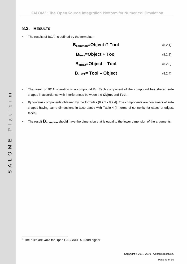
8.2. RESULTS
• The results of BOA1 is defined by the formulas:
Bcommon =Object ∩ Tool (8.2.1)
Bfuse=Object + Tool (8.2.2)
Bcut12=Object – Tool (8.2.3)
Bcut21= Tool – Object (8.2.4)
• The result of BOA operation is a compound Bj . Each component of the compound has shared sub-
shapes in accordance with interferences between the Object and Tool .
• Bj contains components obtained by the formulas (8.2.1 - 8.2.4). The components are containers of sub-
shapes having same dimensions in accordance with Table 4 (in terms of connexity for cases of edges,
faces).
• The result Bcommon should have the dimension that is equal to the lower dimension of the arguments.
1 The rules are valid for Open CASCADE 5.0 and higher

SALOME : The Open Source Integration Platform for Numerical Simulation
Copyright © 2001- 2010. All rights reserved.
Page 41 of 56
SA
LO
ME
P
la
tf
or
m
8.2.1. Example 1
The arguments are (Figure 34)
• Object: edge E1
• Tool: edge E2
Figure 34
The result of BOA operation is compound.
Bcommon The compound contains noting because the dimension of intersection (vertex) is less
than minimal dimension of arguments.
B fuse The compound contains a wire of 4 new edges E11, E12, E21, E22. The edges have one
shared vertex Vn1.
Bcut12 The compound contains a wire of 2 new edges E11, E12. The edges have one shared
vertex Vn1.
Bcut21 The compound contains a wire of 2 new edges E21, E22. The edges have one shared
vertex Vn1.
E1
E2
Vn1
E31
E11
E21
E12
E22
Vn1
E11 E12
Vn1
E31 E21
E22
Bfuse
Bcommon=0
Bcut12
Bcut21

SALOME : The Open Source Integration Platform for Numerical Simulation
Copyright © 2001- 2010. All rights reserved.
Page 42 of 56
SA
LO
ME
P
la
tf
or
m
8.2.2. Example 2
The arguments are (Figure 35):
• Object: edge E1
• Tool: edge E2
Figure 35
The result of BOA operation is compound.
Bcommon The compound contains a wire of 1 new edge E12.
B fuse The compound contains a wire of 3 new edges E11, E12, E13. The edges have shared
vertices.
Bcut12 The compound contains a wire of 1 new edge E11.
Bcut21 The compound contains a wire of 1 new edge E13.
E1
E2
Bfuse
Bcommon
Bcut12
Bcut21
E12
E12
E11
E13
E11
E13

SALOME : The Open Source Integration Platform for Numerical Simulation
Copyright © 2001- 2010. All rights reserved.
Page 43 of 56
SA
LO
ME
P
la
tf
or
m
8.2.3. Example 3
The arguments are (Figure 36)
• Object: face F
• Tool: edge E
Arguments
Bcommon
B fuse=0
Bcut12=0
Bcut21
Figure 36
The result of BOA operation is compound.
Bcommon The compound contains new edge E11.
B fuse The compound contains nothing (different dimensions of the arguments).
Bcut12 The compound contains nothing.
Bcut21 The compound contains new edge E12.
F
E
E11
E12

SALOME : The Open Source Integration Platform for Numerical Simulation
Copyright © 2001- 2010. All rights reserved.
Page 44 of 56
SA
LO
ME
P
la
tf
or
m
8.2.4. Example 4
The arguments are (Figure 37)
• Object: face F1
• Tool: face F2
Arguments
Bcommon
B fuse
F1 F12 F2 F12
F12 F11
F22

SALOME : The Open Source Integration Platform for Numerical Simulation
Copyright © 2001- 2010. All rights reserved.
Page 45 of 56
SA
LO
ME
P
la
tf
or
m
Bcut12
Bcut21
Figure 37
The result of BOA operation is compound.
Bcommon The compound contains new face F12.
B fuse The compound contains a shell of 3 new faces F11, F12, F22.
Bcut12 The compound contains new face F11.
Bcut21 The compound contains new face F22.
F11
F22

SALOME : The Open Source Integration Platform for Numerical Simulation
Copyright © 2001- 2010. All rights reserved.
Page 46 of 56
SA
LO
ME
P
la
tf
or
m
9. LIMITATIONS OF ALGORITHMS
The chapter is devoted to the problems that should be considered as limitations of Algorithms. In most cases
the reason of failure is a superposition of different factors (self-interfered arguments, inappropriate,
ungrounded values of the tolerances of the arguments, adverse mutual position of the arguments, tangency,
etc).
The description below is just to illustrate the limitations and do not exhaust all problems that can be faced in
practice.
Each case of failure of Algorithms is the matter of the maintenance service.
9.1. ARGUMENTS
9.1.1. Common requirements
Each argument should be valid (in terms of BRepCheck_Analyzer), or conversely, if the argument is
considered as not-valid (in terms of BRepCheck_Analyzer), it can not be used as an argument of the
algorithm.
The class BRepCheck_Analyzer is to check the overall validity of a shape. For a shape (or its sub-shapes) to
be valid in Open CASCADE, it must respect certain criteria. If the shape is determined as not valid, the
problems can be fixed by tools from ShapeAnalysis, ShapeUpgrade, ShapeFix packages.
The class BRepCheck_Analyzer is just hand-made tool that has its own problems. Examples of such
problems:
• The Analyzer checks the distances between the two 3D-points Pi, PSi of an edge on a face F. The point
Pi is obtained from 3D-curve (at the parameter ti) of the edge. PSi is obtained from 2D-curve (at the
parameter ti) of the edge on surface S of the face F. To be valid the distance should be less then Tol(E).
The number of these check-points is constant value (say 23). It is supposed that edge E is valid (in terms
of BRepCheck_Analyzer).
• Split the edge E onto two split edges E1, E2. Each split edge has 3D-curve and 2D-curve as the edge E
has. Let’s check E1 (or E2). The Analyzer again checks the distances between the two 3D-points Pi, PSi.
The number of these check-points is again constant value (23). But there are not guarantee that the
distance should be less then Tol(E), because the points for E1 are not the same as for E.
• So, in case when E1 is not valid, the edge E also should not be valid. But E is supposed as valid. Thus
the Analyzer is wrong for E.
The fact that the argument of Algorithm is valid shape (in terms of BRepCheck_Analyzer) is necessary
requirement but not sufficient to produce valid result of the Algorithms.

SALOME : The Open Source Integration Platform for Numerical Simulation
Copyright © 2001- 2010. All rights reserved.
Page 47 of 56
SA
LO
ME
P
la
tf
or
m
9.1.2. Pure self-interference
The argument should not be self-interfered, i.e. all sub-shapes of the argument that have geometrical
coincidence through any topological entities (vertices, edges, faces) should share these entities.
9.1.2.1. Example 1
The compound of two edges E1, E2 (Figure 38) is self-interfered shape and can not be used as the argument
of the Algorithms.
Figure 38
9.1.2.2. Example 2
The edge E (Figure 39) is self-interfered shape and can not be used as the argument of the Algorithms.
Figure 39
9.1.2.3. Example 3
The face F (Figure 40) is self-interfered shape and can not be used as the argument of the Algorithms.
Figure 40
E1
E2
E
F

SALOME : The Open Source Integration Platform for Numerical Simulation
Copyright © 2001- 2010. All rights reserved.
Page 48 of 56
SA
LO
ME
P
la
tf
or
m
9.1.2.4. Example 4
The face F (Figure 42) has been obtained by revolution of the edge E around the line L (Figure 41)
Figure 41 Figure 42
In spite of the fact that the face F is valid (in terms of BRepCheck_Analyzer) the face F is self-interfered
shape and can not be used as the argument of the Algorithms.
E
L
F

SALOME : The Open Source Integration Platform for Numerical Simulation
Copyright © 2001- 2010. All rights reserved.
Page 49 of 56
SA
LO
ME
P
la
tf
or
m
9.1.3. Self-interferences due to tolerances
9.1.3.1. Example 1
The edge E (Figure 43) is based on non-closed circle.
The distance between the vertices of E is D=0.69799.
The values of the tolerances Tol(V1)=Tol(V2)=0.5 (Figure 44).
Figure 43 Figure 44
In spite of the fact that the edge E is valid (in terms of BRepCheck_Analyzer) the edge E is self-interfered
shape because its vertices are interfered. Thus the edge E can not be used as the argument of the
Algorithms.
9.1.3.2. Example 2
The solid S (Figure 45) contains the vertex V. The value of the tolerance Tol(V)= 50.000075982061 (Figure
46). [pkv/901/A9]
Figure 45 Figure 46
In spite of the fact that the solid S is valid (in terms of BRepCheck_Analyzer) the solid S is self-interfered
shape because the vertex V is interfered with a lot of sub-shapes of S without any topological connection
with them. Thus the edge E can not be used as the argument of the Algorithms.
E
E
D
V1
V2
S
V
S
V

SALOME : The Open Source Integration Platform for Numerical Simulation
Copyright © 2001- 2010. All rights reserved.
Page 50 of 56
SA
LO
ME
P
la
tf
or
m
9.1.4. Parametric representation
The parametrization of some surfaces (cylinder, cone, surface of revolution) can be the cause of limitations.
9.1.4.1. Example 1
The parameterization range for cylindrical surface is:
U: [0, 2*π], V: ]-∞, + ∞[ (9.1.4)
The range on U coordinate is always restricted; meanwhile the range on V coordinate is non- restricted.
For clearness
• The face (cylinder-based, radii R=3, H=6) (Figure 47). The Figure 48 shows p-Curves for the cylinder.
Figure 47 Figure 48
• The face (cylinder-based, radii R=3000, H=6000, scale factor ScF=1000) (Figure 49). The Figure 50
shows p-Curves for the cylinder. Please, draw attention on Zoom value on the Figures.
Figure 49 Figure 50

SALOME : The Open Source Integration Platform for Numerical Simulation
Copyright © 2001- 2010. All rights reserved.
Page 51 of 56
SA
LO
ME
P
la
tf
or
m
It is evident that starting with some value of ScF (say ScF>1000000.) all sloped p-Curves on the Figure 48
will be almost vertical (like on the Figure 50). At least there will be not difference between the values of its
angles computed by standard C Run-Time Library functions like double acos(double x). The loss of accuracy
in computation of angles can be the cause of failure of some sub-algorithms of BP (building faces from set of
edges, building solids from set of faces)
9.1.5. Stop-gaps
Due to tolerance model it is possible to create shapes that use sub-shapes of lower order to stop gups.
9.1.5.1. Example 1
The face F has two edges E1, E2 and two vertices, plane {0,0,0, 0,0,1} (Figure 51).
• The edge E1 is based on line {0,0,0, 1,0,0} Tol(E1)=1.e-7.
• The edge E2 is based on line {0,1,0, 1,0,0} Tol(E2)=1.e-7.
• The vertex V1, point {0,0.5,0} Tol(V1)=1.
• The vertex V2, point {10,0.5,0} Tol(V2)=1.
The face F is valid (in terms of BRepCheck_Analyzer).
Figure 51
The values of tolerances Tol(V1), Tol(V2) are big enough to fix the gups between the ends of the edges. But
the vertices V1, V2 does not contain an information about trajectories of connection between corresponding
ends of the edges. The trajectories are undefined. The fact will be the cause of failure of some sub-
algorithms of BP. The sub-algorithms for building faces from set of edges for e.g. use information about all
edges connected in a vertex. The situation when one vertex will have several pairs of edges of kind above
will not be solved in right way.
F
E1 E2
V1
V2

SALOME : The Open Source Integration Platform for Numerical Simulation
Copyright © 2001- 2010. All rights reserved.
Page 52 of 56
SA
LO
ME
P
la
tf
or
m
9.2. INTERSECTION PROBLEMS
9.2.1. Pure intersections and common zones
9.2.1.1. Example 1
Intersection between two edges (Figure 52):
• E1 – based on line: {0,-10,0, 1,0,0} , Tol(E1)=2.
• E2 – based on circle: {0,0,0, 0,0,1}, R=10, Tol(E3)=2.
Figure 52
The result of pure intersection between E1 and E2 is vertex Vx {0,-10,0}.
The result of intersection taking into account tolerances is the common zone CZ (part of 3D-space where the
distance between the curves is less than (or equals to) sum of tolerances of the edges.
As for IP of Algorithms it uses result of pure intersection Vx instead of CZ, because of the reasons:
• The Algorithms does not produce Common Blocks between edges based on underlying curves of
explicitly different type (Line / Circle for this case). The rule of thumb is the following: the different type of
curves is special sign to produce the result of type “vertex”. The rule does not work for non-analytic
curves (Bezier, B-Spline) and theirs combinations with analytic curves.
• The algorithm of intersection between two surfaces (IntPatch_Intersection) does not compute CZ of
intersection curve (-s), point (-s). So even if CZ was computed by Edge/Edge intersection algorithm, its
result could not be treated by Face/Face intersection algorithm.
E2
E1 2*Tol(E1)
2*Tol(E2)
CZ(E1,E2)
Vx

SALOME : The Open Source Integration Platform for Numerical Simulation
Copyright © 2001- 2010. All rights reserved.
Page 53 of 56
SA
LO
ME
P
la
tf
or
m
9.2.2. Tolerances
The limitations are due to modeling errors or inaccuracies.
9.2.2.1. Example 1
The arguments are vertex V1 and edge E2 (Figure 53).
The vertex V1 interferes with the vertex V12. The vertex V1 interferes with the vertex V22.
So the vertex V21 should interfere with the vertex V22.
But it is impossible because the vertices V21, V22 are the vertices of the edge E2, thus V21≠V22.
Figure 53
The problem can not be solved in general, because the length can be as small as possible to provide validity
of E2 (in extreme case: Length (E2)=Tol(V21) + Tol(V22) + ε , ε → 0).
In particular case the problem can be solved by decreasing the values Tol(V21), Tol(V22) Tol(V1) (refinement
of arguments).
It is easy to see that if the E2 were slightly above than tolerance sphere of V1 the problem wouldn’t appear at
all.
V21 V22
E2
V1
Tol(V1)
Tol(V21) Tol(V22)

SALOME : The Open Source Integration Platform for Numerical Simulation
Copyright © 2001- 2010. All rights reserved.
Page 54 of 56
SA
LO
ME
P
la
tf
or
m
9.2.2.2. Example 2
The arguments are two planar rectangular faces F1, F2 (Figure 54).
Intersection curve between the planes is the curve C12. The curve produces new intersection edge EC12.
The edge goes through the vertices V1, V2 thanks to big values of the tolerances of the vertices Tol(V1),
Tol(V2). The situation is: two straight edges (E12, EC12) go through the two vertices. It is impossible for this
case.
Figure 54
The problem can’t be solved in general, because the length of E12 can be infinite and the values of Tol(V1)
and Tol(V2) theoretically can be infinite too.
In particular case the problem can be solved by several ways:
• Decrease if possible the values Tol(V1), Tol(V2) (refinement of F1).
• Analysis of the value of Tol(EC12). Increase Tol(EC12) in order to get common part between the edges
EC12, E12. The common part then will be rejected as already existing edge E12 for the face F1.
It is easy to see that if the C12 were slightly above than tolerance spheres of V1, V2 the problem wouldn’t
appear at all.
V3
Tol(V1)
V2
E12
E23 E41
F1
C12
E34 V4
F2 EC12
V1
Tol(V2)

SALOME : The Open Source Integration Platform for Numerical Simulation
Copyright © 2001- 2010. All rights reserved.
Page 55 of 56
SA
LO
ME
P
la
tf
or
m
9.2.2.3. Example 3
The arguments are two edges E1, E2 (Figure 55):
• The edges E1, E2 have common vertices V1, V2.
• The edges E1, E2 have 3D-curves C1, C2.
• Tol(E1)=1.e-7, Tol(E2)=1.e-7
C1 practically coincides in 3D with C2. The value of deflection is Dmax (say Dmax=1.e-6)
Figure 55
The evident and prospective result should be Common Block between E1, E2. But the result of intersection is
on the Figure 56
Figure 56
The result contains three new vertices Vx1, VX2, Vx3 and 8 new edges (between whiles V1, Vx1, VX2, Vx3, V2)
and no Common Blocks. The result (Figure 56) is quite correct due to source data: Tol(E1)=1.e-7,
Tol(E2)=1.e-7, Dmax=1.e-6.
In particular case the problem can be solved by several ways:
• Increase if possible the values Tol(E1), Tol(E2) to get coincidence in 3D between E1, E2 in terms of
tolerance.
• Replace E1 by more by the more accurate model.
E1
E2
Dmax
V1 V2
C1
C2
E1
E2
2*Tol(E1) 2*Tol(E2)
VX1 VX2 VX3 V1 V2

SALOME : The Open Source Integration Platform for Numerical Simulation
Copyright © 2001- 2010. All rights reserved.
Page 56 of 56
SA
LO
ME
P
la
tf
or
m
The example can be extended from 1D (edges) to 2D (faces) (Figure 57).
Figure 57
The comments and recommendations are the same as for 1D case.
F1
F2
Dmax
S2
Ex1 Ex2 Ex3 E1 E2