General AIMD Congestion Control

General AIMD Congestion Control ∗

Yang Richard Yang, Simon S. Lam

Department of Computer SciencesThe University of Texas at Austin

Austin, TX 78712-1188E-mail: {yangyang,lam }@cs.utexas.edu

Abstract

Instead of the increase-by-one decrease-to-half strategyused in TCP for congestion window adjustment, we con-sider the general strategy such that the increase value anddecrease ratio are parameters. That is, in the congestionavoidance state, the window size is increased byα per win-dow of packets acknowledged and it is decreased toβ ofthe current value when there is congestion indication. Werefer to this window adjustment strategy asgeneral additiveincrease multiplicative decrease(GAIMD). We present the(mean) sending rate of a GAIMD flow as a function ofα, β.We conducted extensive experiments to validate this send-ing rate formula. We found the formula to be quite accuratefor a loss rate of up to 20%. We also present in this paperhow to control flow parameters so that flows with differentparameters can achieve different sending rates. In particu-lar, we present a simple relationship betweenα andβ for aGAIMD flow to beTCP-friendly, that is, for the GAIMDflow to have approximately the same sending rate as aTCP flow under the same path conditions. We present re-sults from simulations in which TCP-friendly GAIMD flows(α = 0.31, β = 7/8) compete for bandwidth with TCPReno flows and with TCP SACK flows, on a DropTail linkas well as on a RED link. We found that the GAIMD flowswere highly TCP-friendly. Furthermore, withβ at 7/8 in-stead of 1/2, these GAIMD flows have reduced rate fluctua-tions compared to TCP flows.

1. Introduction

In a shared network, such as the Internet, end systemsshould react to congestion by adapting their transmission

∗Research sponsored in part by National Science Foundation grant No.ANI-9977267 and grant no. ANI-9506048. Experiments were performedon equipment procured with NSF grant no. CDA-9624082. An early ver-sion of this paper appears inProceedings of ICNP 2000, Osaka, Japan,November 2000.

rates to avoid congestion collapse and keep network uti-lization high [9]. The robustness of the current Internetis due in large part to the end-to-end congestion controlmechanisms of TCP [14]. In particular, TCP uses anaddi-tive increase multiplicative decrease(AIMD) algorithm [5];the TCP sending rate is controlled by a congestion win-dow which is halved for every window of data containinga packet drop, and increased by one packet per window ofdata acknowledged.

Today, a wide variety of new applications such as stream-ing multimedia are being developed to satisfy the growingdemands of Internet users. Many of these new applicationsuse UDP because they do not require reliable delivery andthey are not responsive to network congestion [27]. Thereis great concern that widespread deployment of such unre-sponsive applications may harm the performance of respon-sive TCP applications and ultimately lead to congestion col-lapse of the Internet.

To address this concern one approach is to entice theseapplications to use reservations [7] or differentiated ser-vices [6] that provide QoS. However, even if such servicesbecome available, we expect that many new applicationswill still want to use best-effort service because of its lowcost. A second approach is to promote the use of end-to-endcongestion control mechanisms for best effort traffic and todeploy incentives for its use [9]. However while TCP con-gestion control is appropriate for applications such as bulkdata transfer, many real-time applications would find halv-ing the sending rate of a flow to be too severe a responseto a congestion indication, as it can noticeably reduce theflow’s user-perceived quality [26]. Furthermore, it will beinteresting if we can control service differentiation by usingend-to-end mechanisms, such as by controlling the parame-ters of an end-to-end congestion control protocol.

In the past few years, many unicast congestion controlschemes have been proposed and investigated [13, 17, 29,30, 24, 4, 19, 23, 26, 21, 10, 2]. The common objective ofthese studies is to find a good alternative to the congestioncontrol scheme of TCP. Since the dominant Internet traffic is

TCP-based [28], it is important that new congestion controlschemes beTCP-friendly. By this, we mean that the sendingrate of a non-TCP flow should be approximately the same asthat of a TCP flow under the same conditions of round-triptime and packet loss [17].

The congestion control schemes investigated can be di-vided into two categories: AIMD-based [13, 24, 4, 23, 19]and formula-based [17, 29, 30, 26, 21, 10]. Roughly speak-ing, AIMD-based schemes emulate the increase-by-one anddecrease-to-half window behavior of TCP. Formula-basedschemes use a stochastic model [17, 18, 20] to derive a for-mula that expresses the TCP sending rate as a function ofpacket loss rate, round-trip time, and timeout. Essentially,all of these schemes are based upon the increase-by-one anddecrease-to-half strategy of TCP. We observe that decrease-to-half is not a fundamental requirement of congestion con-trol. In DECbit, also based on AIMD, a flow reduces itssending rate to 7/8 of the old value in response to a packetdrop [16].

In this paper, we consider a more general versionof AIMD than is implemented in TCP; specifically, thesender’s window size is increased byα if there is no packetloss in a round-trip time, and the window size is decreasedto β of current value if there is a triple-duplicate loss in-dication, whereα andβ are parameters. Since the nameAIMD is often used in the literature to refer to TCP Renocongestion control (withα = 1 andβ = 1/2), we call ourapproachgeneral additive increase multiplicative decrease(GAIMD) congestion control.

GAIMD was first considered by Chiu and Jain [5]. Theirstudy is mainly about stability and fairness properties. Theyshowed that ifα andβ satisfy the following relationships,{

0 < α0 < β < 1 (1)

then GAIMD congestion control is “stable” and “fair.”However, their study only considered the case when allflows using the sameα, β parameters. Also, they providedno quantitative study of the effects ofα andβ on perfor-mance metrics. In our study, we consider in detail the rela-tionships between various performance metrics and the pa-rametersα andβ, assuming thatα andβ satisfy (1). In thebalance of this paper, we assume thatα andβ satisfy (1)unless otherwise stated.

In particular, we are interested in the sending rate as asteady state metric, and responsiveness, aggressiveness andrate fluctuations as transient metrics. In this paper, we re-port results on the GAIMD sending rate. Our results ontransient behavior will be reported in [33].

Our first result is a formula showing the GAIMD (mean)sending rate as a function of the control parameters,α andβ, the loss rate, mean round-trip time, mean timeout value,and the number of packets each ACK acknowledges. We

have conducted Internet experiments and extensive simu-lations to validate this formula. The results show that theformula is accurate over a wide range ofα andβ values fora loss rate of up to 20%.

With the formula, we investigate how to chooseα andβsuch that flows with different parameters can achieve differ-ent sending rates. In particular, we obtain our second result:a simple relationship betweenα andβ for a GAIMD flowto be TCP-friendly, that is, for the GAIMD flow to have ap-proximately the same sending rate as that of a TCP flow.The relationship betweenα andβ to be TCP-friendly is

α =4(1− β2)

3

This relationship offers a wide selection of possible valuesfor α andβ to achieve desired transient behaviors, such asresponsiveness and reduced rate fluctuations. For example,we can chooseβ to be 7

8 so that a GAIMD sender has a lessdramatic rate drop than that of TCP given one loss indica-tion. For this choice ofβ, if we useα = 0.31, the GAIMDflow is TCP-friendly.

The balance of this paper is as follows. In Section 2, wepresent the sending rate formula for a GAIMD flow. Exper-iments to validate the formula are also presented in this sec-tion. In Section 3, we use the formula to derive conditionsunder which a GAIMD flow is TCP-friendly. In Section 4,we present experimental results for the TCP-friendlinessconditions. We give a summary of related TCP-friendlycongestion control schemes in Section 5. Conclusion andfuture work are presented in Section 6.

2. Modeling Sending Rate

The motivation of this paper is to consider a generalclass of congestion window adjustment policies. Windowadjustment policy, however, is only one component of acomplete congestion control protocol. Other mechanismssuch as congestion detection and round-trip time estima-tion are needed to make a complete protocol. Since TCPcongestion control has been studied extensively for manyyears, GAIMD adopts these other mechanisms from TCPReno [14, 15, 25, 1]. In the next subsection, we give a briefdescription of the GAIMD congestion window adjustmentalgorithm. All other algorithms are the same as those ofTCP Reno.

2.1. GAIMD congestion window adjustment

A GAIMD session begins in theslowstartstate. In thisstate, the congestion window size is doubled for every win-dow of packets acknowledged. Upon the first congestionindication, the congestion window size is cut in half andthe session enters thecongestion avoidancestate. In this

Tα,β(p, RTT, T0, b) =1

RTT√

2b(1−β)α(1+β) p + T0 min

(1, 3√

(1−β2)b2α p

)p(1 + 32p2)

(2)

state, the congestion window size is increased byα/W foreach new ACK received, whereW is the current conges-tion window size. For convenience, we say that the windowsize is increased byα per round-trip time. So far we haveassumed that the receiver returns one new ACK for eachreceived data packet. Many TCP receiver implementationssend one cumulative ACK for two consecutive packets re-ceived (i.e., delayed ACK [25]). In this case, the windowsize is increased byα/2 per round-trip time. GAIMD re-duces the window size when congestion is detected. Sameas TCP Reno, GAIMD detects congestion by two events:triple-duplicate ACKandtimeout. If congestion is detectedby a triple-duplicate ACK, GAIMD changes the windowsize toβW . If the congestion indication is a timeout, thewindow size is set to1.

2.2. Modeling assumptions

In the Appendix of [34], we derive an analytic expressionfor the sending rate of a GAIMD sender as a function ofα,β, p (loss rate),RTT (round-trip time),T0 (timeout value),andb (number of packets acknowledged by each ACK). Thederivation is a fairly straightforward extension of a similarformula derived for TCP by Padhye, Firoiu, Towsley, andKurose [20]. Various assumptions and simplifications havebeen made in the analysis which are summarized below:

• We assume that the sender always has data to send (i.e.,a saturated sender). The receiver always advertises alarge enough receiver window size such that the sendwindow size is determined by the GAIMD congestionwindow size.

• The sending rate is a random process. We have limitedour efforts to modeling the mean value of the sendingrate. An interesting topic will be to study the varianceof the sending rate which is discussed in [33].

• We focus on GAIMD’s congestion avoidance mecha-nisms. The impact of slowstart has been ignored.

• We model GAIMD’s congestion avoidance behaviorin terms of rounds. A round starts with the back-to-back transmission ofW packets, whereW is the cur-rent window size. Once all packets falling within thecongestion window have been sent in this back-to-backmanner, no more packet is sent until the first ACK is

received for one of theW packets. This ACK recep-tion marks the end of the current round and the begin-ning of the next round. In this model, the duration ofa round is equal to the round-trip time and is assumedto be independent of the window size. Also, it is as-sumed that the time needed to send all of the packetsin a window is smaller than the round-trip time.

• We assume that losses in different rounds are indepen-dent. When a packet in a round is lost, however, weassume all packets following it in the same round arealso lost. Therefore,p is defined to be the probabil-ity that a packet is lost, given that it is either the firstpacket in its round or the preceding packet in its roundis not lost [20].

2.3. Sending rate formula

The analytic expression of Equation (2) for the averageGAIMD sending rateT has been derived (see Appendixof [34] for derivation):

We first observe that the denominator of the formula isthe summation of the following two terms:

TDα,β(p, RTT, b) , RTT

√2b(1− β)α(1 + β)

p (3)

TOα,β(p, T0, b) , T0 min

(1, 3

√(1 − β2)b

2αp

)p(1 + 32p2)

(4)

From the derivation, we know that the denominator consistsof only the first termTDα,β if all congestion indications aretriple-duplicate ACKs; note thatTDα,β does not depend onT0. The second termTOα,β is added when congestion in-dications can be both timeouts and triple-duplicate ACKs;note thatTOα,β does not directly depend onRTT . Com-paring these two terms, we observe that when loss ratep issmall,TDα,β = O(p0.5) andTOα,β = O(p1.5), therefore,TDα,β dominatesTOα,β, and the sending rate is mainlydetermined byTDα,β. However, asp increases,TOα,β be-comes larger. Define

Q , min

(1, 3

√(1 − β2)b

2αp

)

We notice thatQ is the middle term ofTOα,β. From thederivation we know thatQ approximates the probability of aloss being a timeout. From the expression ofQ we note thatwhenp is small, the probability of timeout is low. However,asp increases, the probability of timeout increases rapidlyto 1.

We next consider how the sending rate varies with theparameters,RTT , T0, α, β. It is obvious from Equation(2) that the sending rate decreases with increasingRTT orT0. If β is increased towards 1, bothTDα,β andTOα,β

will decrease, leading to a higher sending rate. Also ifαis increased, bothTDα,β andTOα,β will decrease, leadingto a higher sending rate. Furthermore, we observe thatβmust be less than 1 for the sending rate formula to be valid.If α approaches0, the denominator in Equation (2) goes toinfinity and the sending rate goes to 0.

Lastly, we note that Equation (2) reduces to other well-known TCP formulas when we instantiate it withα = 1 andβ = 1

2 . First, if we ignore theTOα,β term, we obtain

T1, 12(p, RTT, b) = TTCP (p, RTT, b) =

1RTT

√3

2bp

which is the formula derived in [17, 18]. Next, if we includetheTOα,β term, we have

T1, 12(p, RTT, T0, b) =

1

RTT√

2bp3 +T0 min

�1,3√

3bp8

�p(1+32p2)

which is the formula derived in [20]. Therefore, our formulasubsumes these other formulas as special cases.

2.4. Formula validation

Because of the simplicity of GAIMD, we have imple-mented GAIMD in both NetBSD and Linux kernels, andconducted some experiments in a LAN environment. Wehave also tested the formula in Equation (2) extensively us-ing thensnetwork simulator. In all cases, the accuracy ofthe formula is respectable over a wide range ofα and βwhen the loss rate is less than 20%. In this section, we re-port our simulation validations.

The purpose of our validations, presented in this section,is to answer the following questions:

• Is the formula accurate? Over what range of loss ratep is it accurate?

• Since it is a statistical mean, when do sending rate vari-ations become significant?

• What is the general trend when the formula loses ac-curacy?

15Mbps/50msR2R1

TCP s16

TCP s1

GAIMD s1

GAIMD s16

ON/OFF s1

ON/OFF sn

TCP r1

ON/OFF rn

ON/OFF r1

GAIMD r16

GAIMD r1

TCP r16

Figure 1. Simulation topology

2.4.1 Simulation setup

The simulation topology we chose to present results is thewell-known single bottleneck (“dumbbell”) as shown inFigure 1. We have also conducted simulations for othertopologies; the results are similar.

In all of the simulations to be discussed in this section,the bottleneck link bandwidth is fixed at 15Mbps and itspropagation delay at 50ms. We have also conducted exper-iments with other link bandwidths and propagation delays;the results are similar. In all simulations, the access links aresufficiently provisioned to ensure that packet drops/delaysdue to congestion occur only at the bottleneck link fromR1to R2.

We included three types of flows in the simulations. Thefirst type is GAIMD flows. To see sending rate variations,we placed 16 GAIMD flows. For comparison purposes, wealso placed 16 TCP Reno flows. Since the dominant trafficon the Internet is web-like traffic, we believe that it is impor-tant to model the effects of competing web-like traffic (shortTCP connections, some UDP flows). It has been reportedin [22] that WWW-related traffic tends to be self-similarin nature. In [31], it has been shown that self-similar traf-fic can be created by using several ON/OFF UDP sourceswhose ON/OFF times are drawn from a heavy-tailed distri-bution such as the Pareto distribution. Therefore, we choseON/OFF UDP flows as the third type of traffic. In theseexperiments, we set the mean ON time to be 1 second, andthe mean OFF time to be 2 seconds. During ON time eachsource sends at 500Kbps. The shape parameter of the Paretodistribution is set to be 1.5. In our experiments, we variedthe number of ON/OFF sources from 10 to 70 to create aloss rate from about 1% to about 30%.

Another aspect of the simulations worth mentioning ishow we start the flows. To avoid phase effects [11], weassign small random propagation delays to the access linksand start the flows randomly.

In all experiments in this section, each simulation is runfor 120 seconds. The loss rate is approximated by dividingthe number of times a GAIMD flow or TCP flow reduces itswindow size by the total number of packets it sends. Noticethat this estimation of loss rate is a lower bound for the lossrate that we defined in model derivation. Consequently, we

will see that the formula will overestimate and give an upperbound of the sending rate.

2.4.2 Predication accuracy

We first evaluate the predication accuracy of the formula. Agood measure of the accuracy is the ratio of the predicatedsending rate and the actual sending rate. The closer thisratio to 1, the better the predication accuracy. To test thevalidity range of the formula, for eachβ, we varyα from 0.1to 1.0. For eachα, β pair we vary the number of ON/OFFflows from 10 to 70 to create a loss rate from about 1% toabout 30%.

Figures 2, 3, 4 demonstrate the predication accuracy forβ = 0.5, 0.75, 0.875. The bottleneck link is a drop-tail link.In these three figures, the averages of the loss rates, round-trip times, and timeouts of the 16 GAIMD flows in eachexperiment are used to calculate a predicated sending ratefor the experiment. Then the actual sending rates of the16 GAIMD flows are averaged to obtain an average actualsending rate. What the figures show are the ratio betweenthe calculated average sending rate using Equation (2) andthe actual average sending rate. We observe from the fig-ures that for a wide range ofα, β, the formula predicationsare pretty close to the actual sending rate when the loss rateis less than about 20%. Next, we consider the impact of

GAIMD predication accuracy (beta=0.5, drop-tail)

12

510

20 30Loss indication rate (%) 0.2

0.40.6

0.81

alpha

1

Predication/measurement

Figure 2. Accuracy for β = 0.5 and drop-tail


12

510


0.40.6

0.81

alpha

1




12

510


0.40.6

0.81

alpha

1



loss patterns on the accuracy of the formula. In the analyticmodel, we assume that (i) losses in different rounds are in-dependent, and (ii) losses in the same round are correlated,i.e., when one packet is lost, all packets following it in thesame round will also be lost. For a drop-tail router, thiscorrelated-loss assumption is quite reasonable. To see thepotential impact of loss patterns, we repeat the above ex-periments for a RED link. Figure 5 repeats the experimentin Figure 4 but uses a RED link. Comparing Figure 4 and5, we see that loss patterns do not have a large impact onthe accuracy of the formula.

GAIMD predication accuracy (beta=0.875, RED)

12

510


0.40.6

0.81

alpha

1


Figure 5. Accuracy for β = 0.875 and RED2.4.3 Sending rate variation

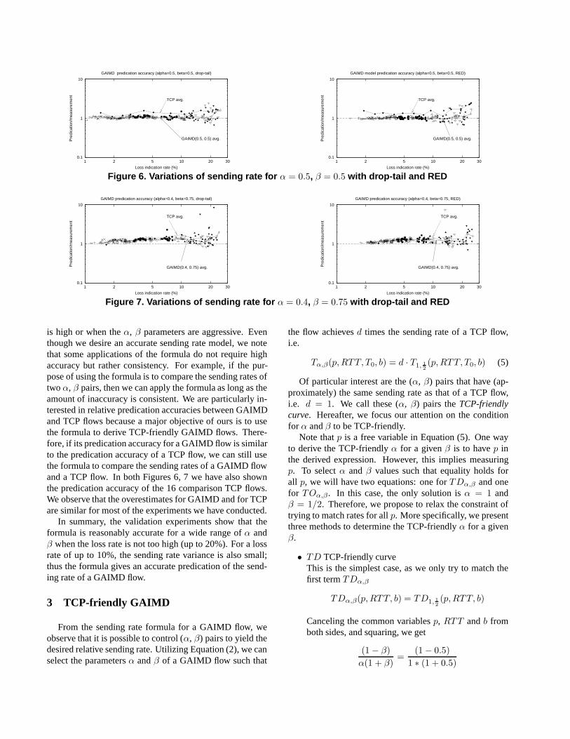
Since what we derived is the mean value of the sending rateas a random process, we expect to see higher variations inthe sending rate when loss rate increases. We illustrate thiseffect in this subsection. In addition to plotting the predi-cation accuracy, Figures 6, 7 show the predication accuracyfor each of the 16 GAIMD flows, forα = 0.5, β = 0.5andα = 0.4, β = 0.75, and for both drop-tail and REDlinks. Observe from the figures that with increasing lossrate, sending rate variations increase. However, from bothfigures we can see that when the loss rate is 10% or less,the predication is accurate and the sending rate variance isreasonably small.

A major trend we observe from all the figures is that thesending rate formula tends to overestimate when loss rate

0.1

1

10

1 2 5 10 20 30

Pre

dica

tion/

mea

sure

men

t

Loss indication rate (%)

GAIMD predication accuracy (alpha=0.5, beta=0.5, drop-tail)

TCP avg.

GAIMD(0.5, 0.5) avg.

0.1

1

10

1 2 5 10 20 30

Pre

dica

tion/

mea

sure

men

t


GAIMD model predication accuracy (alpha=0.5, beta=0.5, RED)

TCP avg.

GAIMD(0.5, 0.5) avg.

Figure 6. Variations of sending rate for α = 0.5, β = 0.5 with drop-tail and RED

0.1

1

10

1 2 5 10 20 30

Pre

dica

tion/

mea

sure

men

t


GAIMD predication accuracy (alpha=0.4, beta=0.75, drop-tail)

TCP avg.

GAIMD(0.4, 0.75) avg.

0.1

1

10

1 2 5 10 20 30

Pre

dica

tion/

mea

sure

men

t


GAIMD predication accuracy (alpha=0.4, beta=0.75, RED)

TCP avg.

GAIMD(0.4, 0.75) avg.

Figure 7. Variations of sending rate for α = 0.4, β = 0.75 with drop-tail and RED

is high or when theα, β parameters are aggressive. Eventhough we desire an accurate sending rate model, we notethat some applications of the formula do not require highaccuracy but rather consistency. For example, if the pur-pose of using the formula is to compare the sending rates oftwo α, β pairs, then we can apply the formula as long as theamount of inaccuracy is consistent. We are particularly in-terested in relative predication accuracies between GAIMDand TCP flows because a major objective of ours is to usethe formula to derive TCP-friendly GAIMD flows. There-fore, if its predication accuracy for a GAIMD flow is similarto the predication accuracy of a TCP flow, we can still usethe formula to compare the sending rates of a GAIMD flowand a TCP flow. In both Figures 6, 7 we have also shownthe predication accuracy of the 16 comparison TCP flows.We observe that the overestimates for GAIMD and for TCPare similar for most of the experiments we have conducted.

In summary, the validation experiments show that theformula is reasonably accurate for a wide range ofα andβ when the loss rate is not too high (up to 20%). For a lossrate of up to 10%, the sending rate variance is also small;thus the formula gives an accurate predication of the send-ing rate of a GAIMD flow.

3 TCP-friendly GAIMD

From the sending rate formula for a GAIMD flow, weobserve that it is possible to control (α, β) pairs to yield thedesired relative sending rate. Utilizing Equation (2), we canselect the parametersα andβ of a GAIMD flow such that

the flow achievesd times the sending rate of a TCP flow,i.e.

Tα,β(p, RTT, T0, b) = d · T1, 12(p, RTT, T0, b) (5)

Of particular interest are the (α, β) pairs that have (ap-proximately) the same sending rate as that of a TCP flow,i.e. d = 1. We call these (α, β) pairs theTCP-friendlycurve. Hereafter, we focus our attention on the conditionfor α andβ to be TCP-friendly.

Note thatp is a free variable in Equation (5). One wayto derive the TCP-friendlyα for a givenβ is to havep inthe derived expression. However, this implies measuringp. To selectα and β values such that equality holds forall p, we will have two equations: one forTDα,β and onefor TOα,β. In this case, the only solution isα = 1 andβ = 1/2. Therefore, we propose to relax the constraint oftrying to match rates for allp. More specifically, we presentthree methods to determine the TCP-friendlyα for a givenβ.

• TD TCP-friendly curveThis is the simplest case, as we only try to match thefirst termTDα,β

TDα,β(p, RTT, b) = TD1,12(p, RTT, b)

Canceling the common variablesp, RTT andb fromboth sides, and squaring, we get

(1 − β)α(1 + β)

=(1 − 0.5)

1 ∗ (1 + 0.5)

Rearranging, we have

α =3(1− β)(1 + β)

(6)

(It is interesting to see that according to Equation (6),for β = 1, we haveα = 0, and forβ > 1, we haveα < 0. Even though these are not stable parameters,the pairing makes sense.)

From both formula derivation and validation, we knowthat compared toTOα,β, TDα,β becomes less impor-tant whenp increases towards 1. Therefore, it may bebetter to try to match theTOα,β term. Thus, a secondequation to determine the TCP-friendlyα for a givenβ is obtained as follows.

• TO TCP-friendly curve

TOα,β(p, T0, b) = TO1, 12(p, T0, b)

Canceling the common variablesp, T0 andb from bothsides, we have√

1 − β2

α=

√1 − 0.52

1

Rearranging, we get

α =4(1− β2)

3(7)

(Notice that forβ = 1, we haveα = 0, and forβ > 1,we haveα < 0, the same pairing as in the previousmethod.)

• Error minimizing TCP-friendly curveThe two previous approaches are based on consider-ing the two terms in the denominator of Equation (2)one at a time. We next consider both terms and useoptimization to findα∗ for a givenβ such that the mis-match between GAIMD and TCP rates is minimizedover a range of loss rates. Formally, we define the er-ror function

Eβ(α) =∫ 1

0

w(p)

∣∣∣∣∣Tα,β(p)T1, 1

2(p)

− 1

∣∣∣∣∣ dp (8)

wherew(p) is a function which allows loss rates thatare important to be given more weight in the optimiza-tion. In this paper, we consider a simple function thatgives a weight of 1 to any loss rate less than a thresh-old value; a loss rate higher than the threshold gets aweight of 0. Figure 8 shows the shape of our weightfunction.

0

1

w(p)

pthreshold

Figure 8. Weight function w(p)

Figure 9 showsEβ(α) for β = 0.875, T0 = 4RTT ,with the weight function threshold varying from 0.1 to0.7. Note thatEβ(α) has a well-defined bottom andthe optimalα∗ for a givenβ is easy to find. We ob-serve the trend that as the weight function thresholdincreases, the optimalα∗ increases. In theβ = 0.875case,α∗ increases from0.26 to about0.3 when theweight function threshold was changed from 0.1 to 0.3.

0

0.05

0.1

0.15

0.2

0.25

0.3

0.35

0.4

0.45

0.5

0.1 0.15 0.2 0.25 0.3 0.35 0.4 0.45 0.5

Inte

grat

ion

of m

issm

atch

alpha

Error integrals (beta=0.875)

threshold=0.1

threshold=0.2

threshold=0.3

Figure 9. Error integral as a function of α

Figure 10 shows TCP-friendly curves obtained by thethree methods described above. There are several inter-esting observations. First we observe that the curve deter-mined byTDα,β is higher than others whenβ is less than0.5, and less than others whenβ is larger than 0.5. Second,we see that the TCP-friendlyα determined byTOα,β givesan upper bound whenβ is larger than 0.5, and the curveis also very close to the one determined by optimization ifthe weight function threshold is above 40%. Therefore, wepropose to use Equation (7) to get the TCP-friendlyα for agivenβ whenever we want to do error minimization up to a40% loss rate.

Figure 11 shows ratios between the sending rates ofGAIMD and TCP Reno for different values of TCP-friendlyα determined by the three methods;β is fixed at 0.875. Weobserve from this figure that at a low loss rate a GAIMDflow using theα determined byTO will receive about20% higher bandwidth than TCP Reno; and the flow us-ing theα determined byTD will receive lower bandwidth.

0

0.2

0.4

0.6

0.8

1

1.2

1.4

1.6

1.8

2

0 0.2 0.4 0.6 0.8 1

alph

a

beta

TCP-friendly curves

TD curve

TO curve

threshold=0.1threshold=0.2threshold=0.3threshold=0.4threshold=0.5

TDTO

Figure 10. TCP-friendly curves

However, the differences diminish as the loss rate becomeshigher. One factor we need to consider when determiningα is that we only compared GAIMD with TCP Reno. How-ever, many variants of TCP, e.g. NewReno, SACK [8], andTCP Vegas [3], achieve higher bandwidth than TCP Reno.Therefore, it is reasonable to select theα that is somewhatmore aggressive than TCP Reno at a low loss rate1. We willsee in the next section that TCP SACK does reduce the ad-vantage of GAIMD when we use theα determined byTO.

We also observe from Figure 11 that when loss rate isvery high, the ratios converge to one because essentially allloss indications are timeouts, and the parametersα andβno longer play an important role. However, as we will seein the next section, under very high loss rate, TCP receivesmore bandwidth than GAIMD because of its more aggres-sive window increasing behavior. This shows that our for-mula loses accuracy when the loss rate is very high.

0.8

0.85

0.9

0.95

1

1.05

1.1

1.15

1.2

0 0.1 0.2 0.3 0.4 0.5 0.6 0.7 0.8

Rat

io

Loss rate (p)

Sending rate relative to TCP at different loss rate (beta=0.875)

TD pair (0.2, 0.875)

TO pair (0.31, 0.875)

th=0.1 pairth=0.2 pairth=0.3 pair

TD pairTO pair

Figure 11. Ratios of the GAIMD flow sendingrate and TCP sending rate

3.1 A closer look at TCP-friendliness

In previous subsections, we derived TCP-friendly curvesusing Equation (2). In this subsection, we provide an in-tuitive explanation of why a GAIMD flow can be TCP-friendly.

1Another possibility is to adaptively changeα by measuring loss rate.

0

5

10

15

20

0 5 10 15 20

GA

IMD

(0.2

, 0

.87

5)

win

do

w s

ize

(p

kt)

TCP window size (pkt)

equal window sizecapacity line

window tracestarting point

steady state line

Figure 12. Window size changing trace

Figure 12 shows the evolution of the window sizes ofa GAIMD(0.2, 7/8) flow and a TCP flow with the sameround-trip time [5]. Since we do not consider timeout, forβ = 7/8, we use the TD curve, and set the value ofα as0.2. The initial window size of the GAIMD(0.2, 7/8) flowis 10, and the initial window size of the TCP flow is 10.Therefore, the starting point of this trace is at (10, 5). Whenthe sum of the window size of the two flows is less than 20,namely the link capacity, the TCP flow will increase its win-dow size by 1 and the GAIMD(0.2, 7/8) flow will increaseby 0.2 per RTT. When the sum is greater than the link ca-pacity, the TCP flow reduces its window size to half, and theGAIMD(0.2, 7/8) flow reduces to 7/8 of the previous value.From this figure, we first observe that the trace will not con-verge to theequal window sizecurve. This means that twoTCP-friendly flows with different control parameters willnot have equal sending rate atany instant of time. We ob-serve, however, that the window size trace crosses the equalwindow size curve. In particular, when the trace is on theleft of the equal window size curve, the GAIMD(0.2, 7/8)flow has a larger window size and therefore will send morepackets. On the other hand, when the trace is on the right ofthe equal window size curve, the TCP flow will send morepackets. As a result, in the long run, they will receive aboutthe same bandwidth. We also observe from this figure thatwhen the flows enter steady states, that is, when the tracefluctuates along the top most line, the oscillation range ofthe GAIMD(0.2, 7/8) flow (projection of the top line on they-axis) is smaller than that of the TCP flow (projection ofthe top line to the x-axis). This result indicates that the ratefluctuations of the GAIMD(0.2, 7/8) flow will be smaller.

4 Experimental Evaluation of GAIMD TCP-friendliness

In this section, we present experimental results for oneparticular GAIMD, namely, forα = 0.31 andβ = 0.875.It will be referred to as GAIMD(0.31, 0.875). We willstudy its performance mainly from the perspective of TCP-friendliness. Results for other TCP-friendly pairs, such asα = 0.58 andβ = 0.75, are similar.

For experiments in this section, we used the topology inFigure 1. However, we used only two types of flows:n TCPReno flows, andn GAIMD(0.31, 0.875) flows. The numbern is varied from 1 to 64. Each simulation was run for 120seconds.

4.1 TCP-friendliness

From the analytic model, we see that loss rate has a ma-jor impact on the sending rate. Therefore, we evaluated theTCP-friendliness of GAIMD(0.31, 0.875) for a wide rangeof loss conditions. There are two experiment parameters wecan use to control the loss rate, namely: the number of flows(2n) and the bottleneck link bandwidth.

0

0.5

1

1.5

2

2.5

3

0 16 32 48 64 80 96 112 128

Nor

mal

ized

sen

ding

rat

e

Total number of GAIMD and TCP flows (2n)

1.5M link (drop-tail), TCP/Reno, GAIMD(0.31, 0.875)

GAIMD(.31, .875) avg.

TCP avg.

GAIMD(0.31, 7/8)TCP

Figure 13. Normalized sending rates for1.5Mbps drop-tail bottleneck link with Reno

0

0.5

1

1.5

2

2.5

3

0 16 32 48 64 80 96 112 128

Nor

mal

ized

sen

ding

rat

e


15M link (drop-tail), TCP/Reno, GAIMD(0.31, 0.875)

GAIMD(.31, .875) avg.

TCP avg.

GAIMD(0.31, 0.875)TCP

Figure 14. Normalized sending rates for15Mbps drop-tail bottleneck link with Reno

Figures 13, 14 show for a drop-tail bottleneck link thenormalized2 average sending rates of GAIMD(0.31, 0.875)and TCP flows, as well as the sending rates of individualflows. We observe that at a low loss rate (15Mbps link, or1.5Mbps link with less than 64 flows), GAIMD(0.31, 0.875)flows receive more bandwidth than TCP flows. This is ex-pected from Figure 11. With a higher loss rate (1.5Mbpslink with more than 64 flows), TCP flows receive higherbandwidth than GAIMD(0.31, 0.875) flows. We have seenconsistently from all of our experiments that at a highloss rate TCP flows receive higher bandwidth than TCP-friendly GAIMD flows. One explanation is that TCP Renoincreases more aggressively under high loss than TCP-friendly GAIMD (i.e., α < 1). Whereas GAIMD’s smallerreduction (i.e.,β > 1/2) does not play as important a rolebecause the congestion window size is small under highloss.

Another observation we can make from these figures isthat the variance of individual flow rates is much higher forthe 1.5Mbps link than for the 15Mbps link. This is expectedbecause we have already seen that sending rate variance in-creases with loss rate increase.

0

0.5

1

1.5

2

2.5

3

0 16 32 48 64 80 96 112 128

Nor

mal

ized

sen

ding

rat

e


1.5M link (RED), TCP/Reno, GAIMD(0.31, 0.875)

TCP avg.

GAIMD(.31, .875) avg.

GAIMD(0.31, 0.875)TCP

Figure 15. Normalized sending rates for1.5Mbps RED link with Reno

0

0.5

1

1.5

2

2.5

3

0 16 32 48 64 80 96 112 128

Nor

mal

ized

sen

ding

rat

e


15M link (RED), TCP/Reno, GAIMD(0.31, 0.875)

TCP avg.

GAIMD(.31, .875) avg.

GAIMD(0.31, 0.875)TCP

Figure 16. Normalized sending rates for15Mbps RED link with Reno

2such that a fair share of the link bandwidth is 1.

We next consider the effects of loss patterns on GAIMDTCP-friendliness. Figures 15 and 16 repeat the experimentsin Figure 13 and 14 with RED links. Comparing the figures,we observe that with RED instead of drop-tail links, TCPreceives higher bandwidth than GAIMD(0.31, 0.875). Weverified this in some other experiments, and it appears thatthe random and early dropping of RED does protect TCPtraffic from less responsive traffic, such as GAIMD(0.31,0.875).

In our third set of experiments, the competing TCP flowsimplement TCP SACK instead of TCP Reno. While it isgenerally assumed that Reno generates the dominant traf-fic in the current Internet, many operating systems are be-ginning to support TCP SACK; for example, Linux kernelsupports TCP SACK as its default. Therefore, we think itis important to evaluate the TCP-friendliness of GAIMDwhen competing with TCP SACK. (We have also experi-mented with the case that GAIMD is based on TCP SACKinstead of Reno. In this case, GAIMD will become moreaggressive.)

0

0.5

1

1.5

2

2.5

3

0 16 32 48 64 80 96 112 128

Nor

mal

ized

sen

ding

rat

e


1.5M link (drop-tail), TCP/Sack, GAIMD(0.31, 0.875)

GAIMD(.31, .875) avg.

TCP avg.

GAIMD(0.31, 0.875)TCP

Figure 17. Normalized sending rates for1.5Mbps drop-tail link with TCP SACK

0

0.5

1

1.5

2

2.5

3

0 16 32 48 64 80 96 112 128

Nor

mal

ized

sen

ding

rat

e


15M link (drop-tail), TCP/Sack, GAIMD(0.31, 0.875)

GAIMD(.31, .875) avg.

TCP avg.

GAIMD(0.31, 0.875)TCP

Figure 18. Normalized sending rates for15Mbps drop-tail link with TCP SACK

Figures 17 and 18 repeat the experiments in Figures 13and 14 except that the competing TCP flows are SACK in-stead of Reno. It can be seen that the results are very similar

to the cases when the competing flows are Reno. However,we do observe that the crossover point in Figure 17 is at alower loss rate than the one in Figure 13 (at 24 flows versus48 flows for a 1.5Mbps drop-tail link).

Figures 19 and 20 repeat the experiments in Figures 15and 16 except that the competing Reno flows are replacedwith SACK flows; we can see that the results are similar tothe previous cases.

0

0.5

1

1.5

2

2.5

3

0 16 32 48 64 80 96 112 128

Nor

mal

ized

sen

ding

rat

e


1.5M link (RED), TCP/Sack, GAIMD(0.31, 0.875)

TCP avg.

GAIMD(.31, .875) avg.

GAIMD(0.31, 0.875)TCP

Figure 19. Normalized sending rates for1.5Mbps RED link with TCP SACK

0

0.5

1

1.5

2

2.5

3

0 16 32 48 64 80 96 112 128

Nor

mal

ized

sen

ding

rat

e


15M link (RED), TCP/Sack, GAIMD(0.31, 0.875)

TCP avg.

GAIMD(.31, .875) avg.

GAIMD(0.31, 0.875)TCP

Figure 20. Normalized sending rates for15Mbps RED link with TCP SACK

To summarize, we see that GAIMD flows compete withboth TCP Reno and TCP SACK flows in a highly friendlymanner over a wide range of loss rates and for both drop-tailand RED queueing disciplines.

4.2 Rate fluctuations

Having investigated long-term sending rate fairness, wenext evaluate the transient behavior of GAIMD. In ourstudy, we are particularly interested in the smoothness ofits sending rate, the convergence speed tofair state and itsresponse to congestion. We observe that a GAIMD flowwith a smaller value ofβ will have a faster response to con-gestion, but its rate fluctuation will be higher. However,

due to space limitation, a detailed discussion of our find-ings is deferred to [33]. Figure 21 shows time traces ofthe sending rates of one GAIMD(0.31, 0.875) flow and oneTCP flow when 4 GAIMD(0.31, 0.875) flows and 4 TCPReno flows share one RED link with 15Mbps bandwidthand 20ms propagation delay. Each point in the figure is cal-culated over a time interval of 150ms, about 2 to 3 timesthe round-trip time. We can observe visually that GAIMD’ssending rate is relatively smooth compared to that of TCP.From [33], we know that if we measure smoothness bysending rate coefficient of variations, GAIMD withβ =7/8 will have about half of the coefficient of variations ofTCP at low loss rate.

0.5

1

1.5

2

2.5

3

3.5

4

4.5

5 10 15 20 25 30 35 40 45 50

Sen

ding

rat

e (M

bps)

Time (sec)

Sending rate changes, 15Mbps RED Link

TCP Reno FlowGAIMD Flow(0.31, 0.875)

Figure 21. GAIMD and TCP sending ratetraces for a 15Mbps RED link

4.3 Implementation

GAIMD is straightforward to implement because weonly need to change two parameters in TCP Reno. Note,however, that we need to distinguish the first loss duringslow start; in this case, the window size is dropped to halfinstead ofβ.

5 Summary of Related Work

AIMD was first proposed by Chiu and Jain in [5]. Thisdesign principle was used in DECbit [16] and TCP [14].One of the first to consider implementing TCP-like conges-tion control for video services is [13]. However, it uses thestandard TCP adjustment rule, and therefore, has the sameTCP rapid rate changes.

Ozdemir and Rhee proposed the TEAR protocol (TCPEmulation at the Receivers) in [19]. In TEAR, a receiveremulates the congestion modifications of a TCP sender.To transform from a window-based scheme to a rate-basedscheme, an weighted sliding window moving average of the

congestion window size is divided by the estimated round-trip time [12]. As we will see in [33], TEAR has some prob-lems in its responsiveness, and aggressiveness behaviors.

Another type of congestion control is to use additive in-crease, multiplicative decrease in some form, but not apply-ing it to a congestion window. The Rate Adaption Protocol(RAP) [23] uses an AIMD rate control scheme based on reg-ular acknowledgments sent by the receiver which the senderuses to detect lost packets and estimate RTT. The authorsuse the ratio between long-term and short-term averages ofRTT to fine tune the sending rate on a per packet basis. Inaddition to the change from a window-based approach toa rate-based approach, RAP also includes a mechanism forthe sender to stop sending in the absence of feedback fromthe receiver. However, RAP does not account for the impactof retransmission timeouts.

Another AIMD protocol is DLA [24] which makes useof RTP reports from the receiver to estimate loss rate andround-trip times.

In equation-based congestion control approaches [17,26, 21, 10], the sender uses an equation that specifies theallowed sending rate as a function of RTT and packet droprate, and adjusts its sending rate as a function of those mea-sured parameters. However, the stability of this particularapproach is not understood yet. Also, measuring loss rateturns out to be a complex issue, especially when the tradeoffbetween responsiveness and accuracy has to be considered.

In [2], Bansal and Balakrishnan use Binomial algorithmsto generalize TCP-style additive-increase by increasing in-versely proportional to a powerk of the current window(for TCP, k=0) and TCP-style multiplicative-decrease bydecreasing proportional to a powerl of the current window(for TCP, l = 1). As we will see in [32], the analysis ofGAIMD and Binomial can be combined to have a more gen-eralized AIMD congestion control.

6 Conclusion

In this paper, we have considered a general version ofAIMD congestion control, where the increase value and de-crease ratio in congestion window adjustment are parame-ters,α andβ, respectively. We derived a simple formulafor the (mean) sending rate of a GAIMD flow as a func-tion of α, β, loss rate, mean round-trip time, mean timeoutvalue, and the number of packets acknowledged by eachACK. Our extensive experiments showed the formula to bequite accurate for a loss rate of up to 20%. We also foundthat we can choose the control parameters to implementend-to-end flow service differentiation. In particular, wepresent in this paper a simple relationship betweenα andβ for a GAIMD flow to be TCP-friendly. We presentedresults from simulations in which TCP-friendly GAIMDflows (α = 0.31, β = 7/8) compete for bandwidth with

TCP Reno flows and with TCP Sack flows, on a DropTaillink as well as on a RED link. We found that the GAIMDflows were highly TCP-friendly. Furthermore, withβ at 7/8instead of 1/2, these GAIMD flows have reduced rate fluc-tuations compared to TCP flows. We are currently investi-gating tradeoffs among rate fluctuation, responsiveness, andconvergence speed. We will report the results in [33].

Acknowledgment

The authors would like to thank Steve Li for valuablediscussions.

References

[1] M. Allman, V. Paxson, and W. Stevens.TCP CongestionControl, RFC 2581, Apr. 1999.

[2] D. Bansal and H. Balakrishnan. TCP-friendly congestioncontrol for real-time streaming applications. Technical Re-port MIT–LCS–TR–806, Massachusetts Institute of Tech-nology, Cambridge, Massachusetts, U.S.A., May 2000.

[3] L. Brakmo, S. O’Malley, and L. Peterson. TCP Vegas: Newtechniques for congestion detection and avoidance. InPro-ceedings of ACM SIGCOMM ’94, Vancouver, Canada, May1994.

[4] S. Cen, C. Pu, and J. Walpole. Flow and congestion con-trol for Internet streaming applications. InProceedings ofMultimedia Computing and Networking 1998, Jan. 1998.

[5] D.-M. Chiu and R. Jain. Analysis of the increase and de-crease algorithms for congestion avoidance in computer net-works. Computer Networks and ISDN Systems, 17, June1989.

[6] D. Clark and J. Wroclawski. An approach to service alloca-tion in the Internet. work in progress (IETF Internet-Draft),July 1997.

[7] D. D. Clark, S. Shenker, and L. Zhang. Supporting real-time applications in an Integrated Services Packet Network:architecture and mechanism. InProceedings of ACM SIG-COMM ’92, July 1992.

[8] K. Fall and S. Floyd. Simulation-based comparisons ofTahoe, Reno, and SACK TCP.ACM Communications Re-view, 26(3):5–21, July 1996.

[9] S. Floyd and K. Fall. Promoting the use of end-to-end con-gestion control in the Internet.IEEE/ACM Transactions onNetworking, 7(4), Aug. 1999.

[10] S. Floyd, M. Handley, J. Padhye, and J. Widmer. Equation-based congestion control for unicast applications. InPro-ceedings of ACM SIGCOMM 2000, Aug. 2000.

[11] S. Floyd and V. Jacobson. On traffic phase effects in packet-switched gateways.Internetworking: Research and Experi-ence, 3(3), Sept. 1992.

[12] J. Golestani and K. Sabnani. Fundamental observations onmulticast congestion control in the Internet. InProceedingsof IEEE INFOCOM ’99, 1999.

[13] S. Jacobs and A. Eleftheriadis. Providing video services overnetworks without quality of service guarantees. InProceed-ings of World Wide Web Consortium Workshop on Real-timeMultimedia and the Web, Oct. 1996.

[14] V. Jacobson. Congestion avoidance and control. InProceed-ings of ACM SIGCOMM ’88, Aug. 1988.

[15] V. Jacobson. Modified TCP congestion avoidance algorithm.Note sent to end2end-interest mailing list, 1990.

[16] R. Jain, K. K. Ramakrishnan, and D.-M. Chiu. Congestionavoidance in computer networks with a connectionless net-work layer. Technical Report DEC–TR–506, DEC, Aug.1987.

[17] J. Mahdavi and S. Floyd. TCP-friendly unicast rate-basedflow control. Note sent to the end2end-interest mailing list,1997.

[18] M. Mathis, J. Semke, J. Mahdavi, and T. Ott. The macro-scopic behavior of the TCP congestion avoidance algorithm.ACM Computer Communication Review, 27(3):67–82, July1997.

[19] V. Ozdemir and I. Rhee. TCP emulation at the receivers(TEAR), presentation at the rm meeting, Nov. 1999.

[20] J. Padhye, V. Firoiu, D. Towsley, and J. Kurose. ModelingTCP throughput: a simple model and its empirical valida-tion. In Proceedings of ACM SIGCOMM ’98, Vancouver,B.C., Sept. 1998.

[21] J. Padhye, J. Kurose, D. Towsley, and R. Koodli. A modelbased TCP-friendly rate control protocol. InProceedings ofNOSSDAV ’99, June 1999.

[22] K. Park, G. Kim, and M. Crovella. On the relationship be-tween file sizes, transport protocols and self-similar networktraffic. In Proceedings of IEEE ICNP ’96, 1996.

[23] R. Rejaie, M. Handley, and D. Estrin. RAP: An end-to-end rate-based congestion control mechanism for realtimestreams in the Internet. InProceedings of IEEE INFOCOM’99, volume 3, Mar. 1999.

[24] D. Sisalem and H. Schulzrinne. The loss-delay based ad-justment algorithm: A TCP-friendly adaptation scheme. InProceedings of NOSSDAV ’98, July 1998.

[25] W. Stevens.TCP/IP Illustrated, Volume 1: The Protocols.Addison-Wesley, 1997.

[26] W.-T. Tan and A. Zakhor. Real-time Internet video usingerror resilient scalable compression and TCP-friendly trans-port protocol.IEEE Trans. on Multimedia, 1, June 1999.

[27] V. Thomas. IP multicast in RealSystem G2. Whitepaper, RealNetworks, Jan. 1998. Available athttp://service.real.com/.

[28] K. Thompson, G. J. Miller, and R. Wilder. Wide-area Inter-net traffic patterns and characteristics.IEEE Network, 11(6),Nov. 1997.

[29] T. Turletti, S. F. Parisis, and J.-C. Bolot. Experiments witha layered transmission scheme over the Internet. ResearchReport No 3296, INRIA, Nov. 1997.

[30] L. Vicisano, L. Rizzo, and J. Crowcroft. TCP-like conges-tion control for layered multicast data transfer. InProceed-ings of IEEE INFOCOM ’99, volume 3, Mar. 1999.

[31] W. Willinger, M. Taqqu, R. Sherman, and D. Wilson. Self-similarity through high variability: statistical analysis ofEthernet LAN traffic at the source level. InProceedings ofACM SIGCOMM ’95, 1995.

[32] Y. R. Yang, M. S. Kim, and S. S. Lam. Analysis of Bino-mial congestion control. Technical Report TR–00–14, TheUniversity of Texas at Austin, June 2000.

[33] Y. R. Yang, M. S. Kim, and S. S. Lam. Transient behav-iors of TCP-friendly congestion control protocols. TechnicalReport TR–00–23, Department of Computer Sciences, TheUniversity of Texas, Austin, Texas, U.S.A., Sept. 2000.

[34] Y. R. Yang and S. S. Lam. General AIMD congestion con-trol. Technical Report TR–00–09, Department of ComputerSciences, The University of Texas, Austin, Texas, U.S.A.,May 2000.

Documents

General AIMD Congestion Control