Embed Size (px)
Citation preview

Gene Expression Data Analyses
(2)
Trupti Joshi
Computer Science Department317 Engineering Building North
E-mail: [email protected](O)

Recap (Lecture 1) RNA is first isolated from different tissues, developmental stages,
disease states or samples subjected to appropriate treatments.
RNA is then labeled and hybridized to the arrays using an experimental strategy that allows expression to be assayed and compared between appropriate sample pairs.
Use a single label and independent arrays for each sample, or a single array with distinguishable fluorescent dye labels for the individual RNAs.
Regardless of the approach chosen, the arrays are scanned after hybridization and independent grayscale images, typically 16-bit TIFF images, are generated for each pair of samples to be compared.
Images are then analyzed to identify the arrayed spots and to measure the relative fluorescence intensities for each element.

Lecture Outline
Image analysis
Data representation
Data Normalization Normalization within slides
Scaled normalization
Linear regression normalization
Lowess Normalization
Global vs. Local normalization
Variance regularization
Replicate Filtering
Normalization between slides

Lecture Outline
Image analysis
Data representation
Data Normalization Normalization within slides
Scaled normalization
Linear regression normalization
Lowess Normalization
Global vs. Local normalization
Variance regularization
Replicate Filtering
Normalization between slides

Spotted Array
Cy5 Cy3

Quality of Images
Common problems:Spot is not regular (e.g. not round, donut shape)Hybridization is not even (e.g. half is good)Hybridization with fogThe hybridization is too weak or saturated

Image Processing
GriddingIdentifying spot locations
SegmentationIdentifying foreground and background
Processing techniquesManual vs. semiautomatic gridding
Variety of segmentation techniques

Segmentation

Data Quality (1)
Irregular size or shape Irregular placement Low intensity
Saturation Spot variance Background variance
indistinguishable saturated bad print artifactmiss alignment

Calculate numeric characteristics of each spot
Throw out spots that do not meet minimum requirements for each characteristic
Throw out spots that do not have minimum overall combined quality
Data Quality (2)
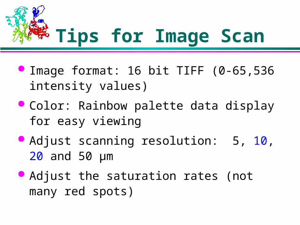
Tips for Image Scan
Image format: 16 bit TIFF (0-65,536 intensity values)
Color: Rainbow palette data display for easy viewing
Adjust scanning resolution: 5, 10, 20 and 50 µm
Adjust the saturation rates (not many red spots)

Signal Extraction
Many softwares are available (Imagene, GPC VisualGrid, TIGR SpotFinder, etc)
Most of them are effective

Tips for Signal Extraction
Signal/noise ratio>+1.96 Background area selection Spot finding automation Batch processing ability might not be good Bad spots should be removed

Lecture Outline
Image analysis
Data representation
Data Normalization Normalization within slides
Scaled normalization
Linear regression normalization
Lowess Normalization
Global vs. Local normalization
Variance regularization
Replicate Filtering
Normalization between slides

Expression Ratio Consider an array that has Narray distinct elements, and
compare a query (R) and a reference sample (G), (for the red and green colors commonly used to represent array data), then the ratio (T) for the ith gene (where i is an index running over all the arrayed genes from 1 to Narray):
Usually use log2(Ti)Reflect the up-regulated and down-regulated genes

Log Transformations Logarithm base 2 transformation, has the advantage of
producing a continuous spectrum of values and treating up and down regulated genes in a similar fashion.
The logarithms of the expression ratios are also treated symmetrically, such that genes up regulated by a factor of 2 has a log2(ratio) of 1, gene down regulated by a factor of 2 has a log2(ratio) of −1, gene expressed at a constant level (ratio of 1) has a log2(ratio) equal to
zero.

Example
Gene 1 2 3 4 5
R: Cy3: 0.1, 0.6, 0.3, 0.3, 0.5 G: Cy5: 0.2, 0.3, 0.6, 0.2, 0.5
Thus
Gene 1: log2(0.1/0.2) = -1
Gene 2: log2(0.6/0.3) = 1
…..
Gene 4: log2(0.3/0.2) = 0.58
…

Lecture Outline
Image analysis
Data representation
Data Normalization Normalization within slides
Scaled normalization
Linear regression normalization
Lowess Normalization
Global vs. Local normalization
Variance regularization
Replicate Filtering
Normalization between slides

Data Normalization
Calibrated, red and green equally detectedUncalibrated, red light under detected

Rational for Data Normalization
Unequal quantities of starting RNA Differences in labeling Differences in detecting efficiencies
between the fluorescent dyes Scanning saturation Systematic biases in the measured
expression levels

Two normalization
Normalization within slides Normalization between slides

Normalization Benefits
Can control for many of the experimental sources of variability (systematic, not random or gene specific)
Bring each image to the same average brightness
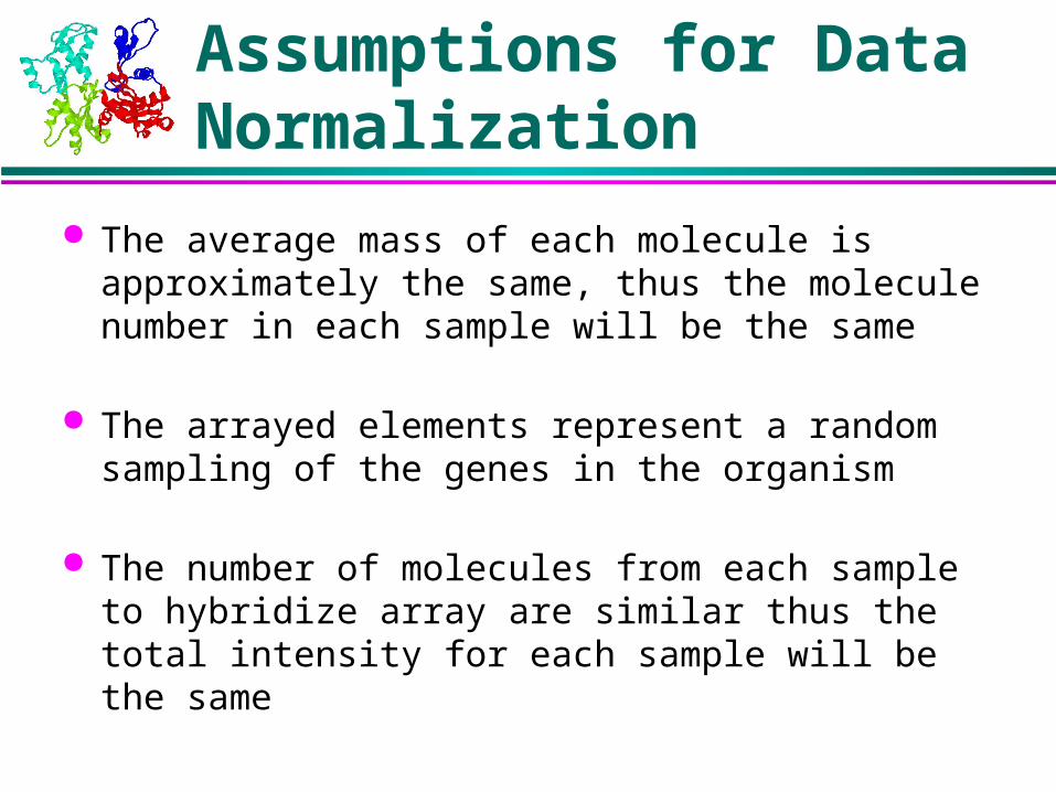
Assumptions for Data Normalization
The average mass of each molecule is approximately the same, thus the molecule number in each sample will be the same
The arrayed elements represent a random sampling of the genes in the organism
The number of molecules from each sample to hybridize array are similar thus the total intensity for each sample will be the same

Lecture Outline
Image analysis
Data representation
Data Normalization Normalization within slides
Scaled normalization
Linear regression normalization
Lowess Normalization
Global vs. Local normalization
Variance regularization
Replicate Filtering
Normalization between slides

Data Normalization Methods
Scaled NormalizationBy total intensityBy meanBy medianBy a group of genes
Linear regression analysis Lowess normalization Log centering Rank invariant methods Chen’s ratio statistics

Scaled Normalization by Total Intensity
Gi and Ri are the measured intensities for the ith array element
Log2(Ti’) is the normalized value

Example
Gene 1 2 3 4 5
R: Cy3: 0.1, 0.2, 0.3, 0.3, 0.5 G: Cy5: 0.2, 0.5, 0.6, 0.2, 0.5Ntotal = (0.1+0.2+0.3+0.3+0.5)/(0.2+0.5+0.6+0.2+0.5)
=1.4/2
=0.7
Thus gene 1: log2(0.5)-log2(0.7)
…

Other Scaled Normalization
Substitute the Ntotal by Nmean, Nmedian
For the normalization for a subset of genes, use the values generated from a subset of genes instead of all genes during the transformation

Regression Normalization
Fit the linear regression model: Assumption: all the genes on the array have the
same variance (homogeneity)
Test the significance of the intercept . Fit a linear regression without if it is insignificant.
Transform the treatment data: Problem:
assumption may not hold
nonlinear trend (the third replicates of RL95 data has a slight quadratic trend) .
iii xy
ii
yy

Scatter Plot of Log Intensity before vs. after Regression Normalization
2 3 4 5 6 7
23
45
67
scatter plot of DMSO vs BAP
log(dmso1)
log(b
ap1)
2 3 4 5 6 7 8
24
68
scatter plot of DMSO vs BAP
log(dmso2)
log(b
ap2)
0 2 4 6 8
13
57
scatter plot of DMSO vs BAP
log(dmso3)
log(b
ap3)
2 3 4 5 6 7
23
45
67
scatter plot after norm
log(dmso1)
log(b
ap1)
2 3 4 5 6 7 82
46
8
scatter plot after norm
log(dmso2)
log(b
ap2)
2 3 4 5 6 7 8
13
57
scatter plot after norm
log(dmso3)
log(b
ap3)

Problem for Above Normalization
Only take care of the intensities between channel
Do not take into account systematic bias that may appear within the dataThe log2(ratio) values can have a systematic
dependence on intensity most commonly a deviation from zero for low-intensity spots.

Systematic Intensity-dependent Effects of log2(ratio)
Examples: Under-expressed genes appear up-regulated in the red channel. Moderately expressed genes appear up-regulated in the green channel.
Explanation: Chemical dyes don’t fluoresce equally at different levels because of different levels of quenching (a phenomenon where dye molecules in close proximity, re-absorb light from each other, thus diminishing the signal)
Solution: Easiest way to visualize intensity-dependent effects is to plot the measured log2(Ri/Gi) for each element on the array as a function of the log2(Ri*Gi) product intensities.
Such 'R-I' (for ratio-intensity) plot can reveal intensity-specific artifacts in the log2(ratio) measurements.

R-I Plots
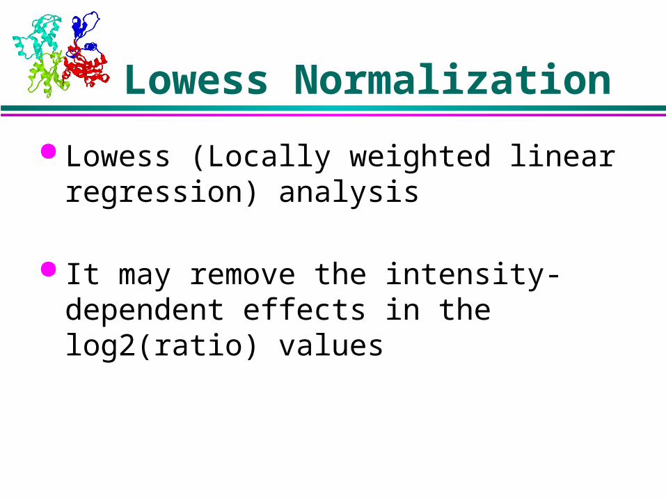
Lowess Normalization
Lowess (Locally weighted linear regression) analysis
It may remove the intensity-dependent effects in the log2(ratio) values
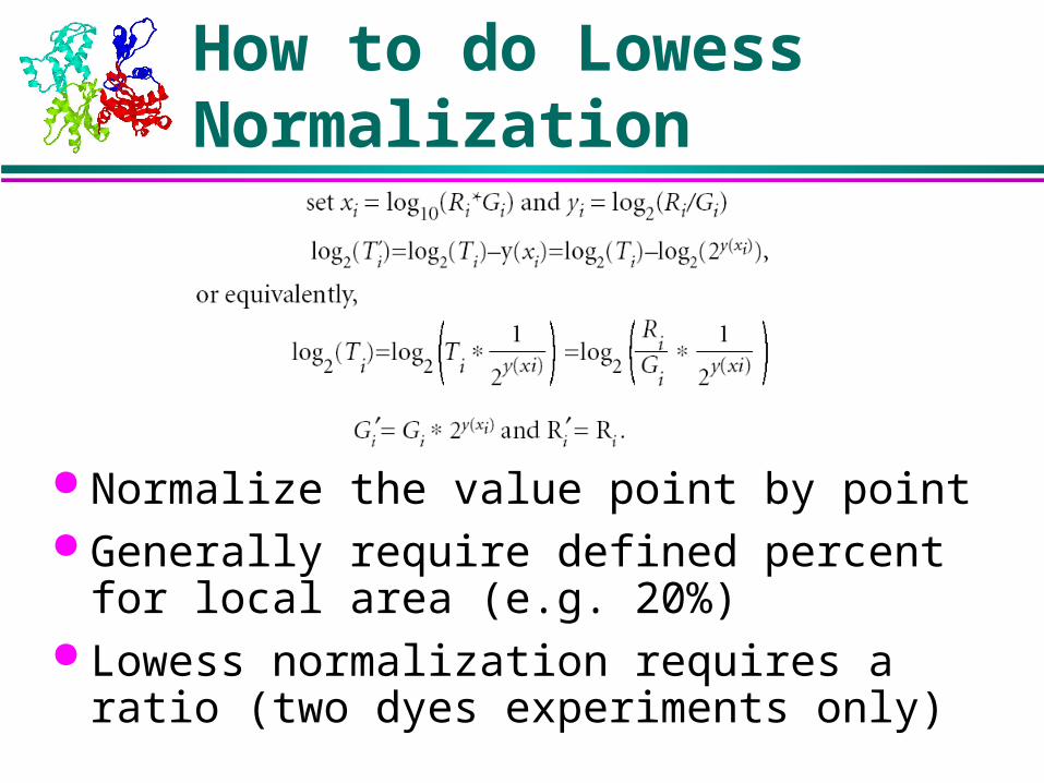
How to do Lowess Normalization
Normalize the value point by point Generally require defined percent for local
area (e.g. 20%) Lowess normalization requires a ratio (two
dyes experiments only)

Effects of Lowess Normalization on R-I Plot

Globe vs Local Normalization
The pin may generate some bias: one region has a larger spots.
Problem: May cause variance of one region to be different from that of another region

Variance Regularization
Assume that each subgrid has M elements, (with mean of the log2(ratio) values in each subgrid already adjusted to zero), then variance in the nth subgrid is
If the number of subgrids in the array is Ngrids, then the appropriate scaling factor for the elements of the kth subgrid is
Scaling all of the elements within the kth subgrid by dividing by the same value ak computed for that subgrid
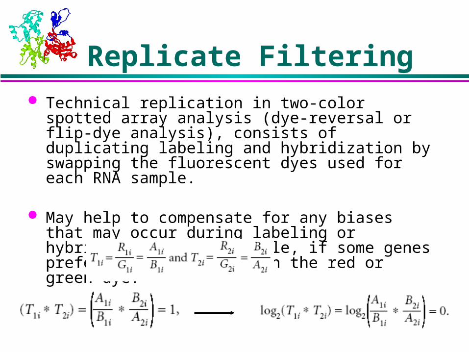
Replicate Filtering Technical replication in two-color spotted array analysis
(dye-reversal or flip-dye analysis), consists of duplicating labeling and hybridization by swapping the fluorescent dyes used for each RNA sample.
May help to compensate for any biases that may occur during labeling or hybridization; for example, if some genes preferentially label with the red or green dye.

Replicate Filtering
Outliers excluded

Lecture Outline
Image analysis
Data representation
Data Normalization Normalization within slides
Scaled normalization
Linear regression normalization
Lowess Normalization
Global vs. Local normalization
Variance regularization
Replicate Filtering
Normalization between slides

Normalization between slides
Use scaled normalization
Generally preferred medium for normalization
Lecture Outline
Image analysis
Data representation
Data Normalization Normalization within slides
Scaled normalization
Linear regression normalization
Lowess Normalization
Global vs. Local normalization
Variance regularization
Replicate Filtering
Normalization between slides

Reading Assignments
Suggested reading: Quackenbush J. Microarray data normalization and
transformation. 2002. Nature Genetics, 32: 496-501.
Yang YH, Dudoit S, Luu P, Lin DM, Peng V, Ngai J, Speed TP. 2002. Normalization for cDNA microarray data: a robust composite method addressing single and multiple slide systematic variation. Nucleic Acids Res. 30: e15.