Embed Size (px)
Citation preview
Gendered Economic Policy Making: The Case of Public
Expenditures on Family Allowances
Oznur Ozdamar
Bologna University, Department of Economics
Strada Maggiore, 45
40125 Bologna (Italy)
Abstract
Parliament is the place where politicians make laws to set the policy direction of countries. Non-
involvement of different voices such as gender, race and ethnicity in policy decisions may create an
inequality in policy-making. Regarding gender, previous literature suggests that women and men may
have different policy preferences and women give more priority to policies related to their traditional
roles as care givers to children in the family. Public spending on family allowances is one of the economic
policies that plays an important role in helping families for the childcare. This paper contributes to the
literature by analyzing the relationship between female political representation and public spending on
family allowances within a perspective of critical-mass framework.
JEL-Classification: H53, H83, J16
Keywords: Women in Economic Policy-Making, Public Expenditures on Family Allowances, Critical Mass,
Panel Data Analysis
1
1 Introduction
The participation of citizens in public policy-making process comes in two forms: a)Direct democracy :
Direct participation of citizens in government affairs b)Indirect democracy : Indirect participation through
representatives who are elected in elections. In line with the global trend to democratization, it has highly
emphasized that the direct or the indirect political participation must cover diverse groups irrespective of
race, class and gender (Guinier, 1994; Lijphart, 2012). The failure of involving different groups in policy-
making may prove the existence of an inequality in political decisions related to public policy-making. Among
these categories, in recent decades, the question of female political participation has emerged as a global
issue in all over the world.
Over the last ten years, therefore, scholars have engaged in theoretical and empirical discussions on
female participation in politics and ask whether there is a link between the number of female politicians
and allocation of public resources to women’s policy preferences (Phillips, 1995; Young, 2002). Contrary to
unitary models, non-unitary models in family economics1 suppose that differences in preferences of men and
women influence the choices of families and women often have stronger preferences on childcare and child
raising issues. The empirical studies also often emphasize on the preference differences between sexes. Their
common argument is that women are more likely than man invest in children and favour redistribution and
they give priority to public policies related to their traditional roles as care givers in the family and society
(Besley and Case, 2000; Case and Deaton, 1998; Alesina and La Ferrara, 2005; Thomas, 1990; Duflo, 2003;
Edlund and Pande, 2002; Chattopadhyay and Duflo, 2004). Such sex differences are now leading to promotion
of gender equality as a potent means of human development2(Duflo, 2012; UN, 2013). The gender differences
in preferences within the society and the family may also be brought into political institutions, influencing
the voting behaviour of politicians, therefore, the allocation of resources across spending categories.
To investigate the role of female politicians in policy making, scholars have empirically analyzed the
relationship between the fraction of female politicians in politics and various public spending categories.
Considering the existing studies in the empirical literature, findings for the effect of the gender specific
decisions on the governance of public spending is mixed so far. On one hand, it has been argued that female
politicians contribute to an increase in public spending that concerns women’s preferences. On the other
hand, some studies find no evidence that such policies are significantly affected by the gender of politicians.
1For more detailed information,see; Manser and Brown (1980); McElroy and Horney (1981); Lundberg and Pollak (1993).2For instance, conditional cash transfers (CCT), which have recently been launched in many countries, target regular
enrollment of the children into schools and getting regular health controls in the health centers (e.g receiving vaccinations).Considering the fact that women have higher tendency to spend for children in families, CCT qualify only mothers.
2
Theoretical literature also has diverging arguments on the importance of the identity of the politician in
shaping the allocation of resources across spending categories. In contrast to Downs (1957)’s Median Voter
Theorem, Citizen Candidate Models (Osborne and Slivinski, 1996; Besley and Coate, 1997) support the fact
that the identity and preferences of a politician matters for the implementation of a policy.
This paper empirically tests the validity of these two alternative theories and contributes to the strand of
literature by studying the relationship between female political participation and public spending on family
allowances across OECD countries. Public spending on family allowances is one of the family-specific policies
that plays an important role in helping families for the child raising which the literature suggests is one of
the woman’s primary concerns.
The preliminary result of this paper is the lack of a relationship between the female political participation
and public spending on family allowances. That result can be interpreted in three ways.
• Median Voter Theorem may apply rather than Citizen Candidate Models.
According to Median Voter Theorem, if candidates are office-seeking, they commit to implement only specific
policies which reflect the preferences of the median voters (Downs, 1957), namely preferences and identities
of the politicians do not matter in public policy making.
Most of the social spending goes to the old-age benefits and pensions over the forty years across OECD
countries. The rapid growth in these spending categories is mainly due to the structural factors such as
population ageing . Although the recent economic crisis (2007/08) has made an increase on family-specific
spending with an idea to support future generations, social spending on the elderly amounted to 11% of GDP
which is exactly half of the overall social welfare spending (22% of GDP) in 2009. 7% of the total is the share
of public health expenditures and the remaining 4% of total social spending is shared by unemployment,
housing, spending on active labor market programs and spending on families (OECD, 2013, 2012). The
disparity in the resource allocation within social welfare areas might be a rational response by vote-seeking
politicians due the population of many OECD countries is getting older and those are with the greatest
propensity to vote3.
• Preferences and the gender identity of politicians might still matter for the policy determination but
3Moreover, electoral participation is falling fastest among the young across the OECD countries, which gives a greaterinfluence to older voters on political decisions. For instance, in 2010 British general election, just 44% of young people agedat 18-24 voted compared to 76% of those aged over 65. In general, older people are much more likely to vote than youngerpeople across OECD countries (Diamond and Lodge, 2013). Among the OECD-34 countries, Italy, Belgium and Australia arethe only countries with a small tendency for the young people to vote more than the old people. The higher participationof elderly people in national elections, as well as the growing share of the elderly population may also influence the politicalprocess, as introducing budget cuts in social welfare spending that unequally benefit the old. In 2011, the average percentagepoint difference in voting rates between those aged over 55 years old and those aged between 16-35 years old was 12.1% in theOECD (OECD, 2011).
3
the preferences of the women who involved in political activities might be close to those of their male
colleagues.
• Gender identity of the politician might matter but the ineffectiveness of the female political participation
on policy-decision making and the insufficient allocation towards family allowances may depend on the
under-representation of women in political institutions.
Namely, the role of female politicians may start to be relevant in terms of bargaining power over policy
making when the percentage share of the female politicians reach a given critical mass threshold.
Therefore, I have further aimed to analyze whether this lack of a relationship may turn to be a significant
relationship after the number of female politicians reach a critical mass threshold in terms of bargaining
power in policy making. Accordingly, the secondary result of the paper shows that a simple positive re-
lationship between the fraction of female parliamentarians and the public spending on family allowances
exists only when a critical mass threshold is passed. However,even though they are over a certain critical
mass threshold, female parliamentarians under majority governments would reflect the preferences of median
voters rather than the preferences of their own interest groups, in contrast to female parliamentarians in
coalition governments.
The paper is organized as follows: section 2 discusses the theoretical background and presents recent
empirical studies on the relationship between female political participation and public policies. Section 3
presents the data, section 4 specifies the empirical model and presents results. Finally, section 5 investigates
the robustness of the relevant results and section 6 concludes.
2 Theoretical Background and Existing Studies
This paper tests the validity of two theories (Citizen Candidate Models versus Median Voter Theorem).
Citizen Candidate Models of Political Economy claims that the identity or preferences of a politician matters
for the policy determination (Besley and Coate, 1997; Osborne and Slivinski, 1996). If politicians can
not commit on moderate policies before being elected, the identity and the individual preferences of the
politician matters for the policy determination rather than the preferences of the median voter. These
models assume that existing political institutions cannot enforce full policy commitment and an increase
in political participation afforded to a disadvantaged group will enhance its influence on a specific policy.
Namely, the political participation of disadvantaged groups such as women, poor or ethnic minorities can
translate into public policy outcomes which reflect the preferences of such groups. For instance Pande (2003)
4
has pointed out that policies chosen by minority politicians reflect the policy preferences of those minorities.
Her empirical results show that the increasing proportions of the minority participation increase the level
of transfers going to this group. Similarly, the political participation of women may translate into a public
policy which reflects women’s preferences.
Existing single-country studies on the relationship between female political participation and policies
that concern women’s interests have heterogeneous results. Thomas (1991), using data gathered from a
survey(1981) on members of the lower houses of the state legislatures of the twelve US states, reveals that
states with the highest percentages of female representatives introduce more priority bills dealing with issues
of women and children. Correspondingly, employing data on the bill introduction in Argentine Chamber
of Deputies and the U.S House of Representatives, Jones (1997) has found that the gender of legislators
matter in investing on the areas concern women rights, families and children. Moreover, Wangnerud (2009),
using parliamentary surveys carried out in the Swedish Parliament, has emphasized on the necessity of
female participation to take into account women’s interests in policy-making. Her findings show that female
members of the parliament address issues of social welfare policies such as family more than their male
colleagues. A more recent work on Swedish municipalities by Svaleryd (2009) has found a positive impact of
the female political participation on public spending towards education and childcare. Similarly Lovenduski
and Norris (2003), using a survey from 2001 British Representation Study of 1,000 national politicians, have
emphasized on the sex differences of legislators in policy making related to women’s issues. One of the other
applications to this line of models has been done by Chattopadhyay and Duflo (2004) who have carried on
a survey for all investments in local public goods in sample villages of two districts in India. They have
found that, female members of reserved village councils make more investment in drinking water than male
members in where women complain more often then men about drinking water. Rehavi (2007), similarly
with Dodson and Carroll (1991) has found a dramatic movement of women into US State Legislators over
the past quarter century for a robustly significant 15% share of the rise in state health spending. In contrast
to these single-country findings, a recent working paper by Ashworth et al. (2012) on Flemish Municipalities
has found a contradictory result claiming that higher female participation to the local parliaments is not
associated with higher spending levels. Furthermore, applying an empirical study on Italian municipalities,
Rigon and Tanzi (2011) has found no evidence on a significant relationship between female politicians and
social expenditures until the number of female politicians reach a critical mass threshold. According to them,
this result indicates that even though Italy is one of the most developed countries, there are still very few
numbers of female politicians in the parliament or municipal councils.
5
Although existing single-country studies have ambigious results, empirical macro level studies have so
far agreed on the positive effectiveness of the female politicians on various policy outcomes such as social
welfare spending, health spending, spending on maternity and parental benefits and education expenditures.
Bolzendahl and Brooks (2007) investigates the influence of female parliamentarians on social welfare spending
in national legislatures within 12 capitalist democracies during the period from 1980 to 1999. They have
found a strong support for the hypothesis that female political participation increases social welfare spending.
Analyzing the impact of female representation in the legislative power on different policy outcomes including
health, education, social welfare spending, Chen (2010) finds a positive effect of the female legislators on
the government expenditures of social welfare. Bonoli and Reber (2010) find a strong impact of women’s
presence in parliament on total public family expenditures using fixed effects model. Kittilson (2008), with
systematic analyses of 19 OECD countries between 1970 and 2000, has showed that women’s parliamentary
presence significantly influences the maternal and parental leave policies. Using a dataset of 80 countries in
the year 2000, Mavisakalyan (2014) has quantified the implications of women’s cabinet representation for
public health policy outcomes. Her main finding is that a higher share of women in cabinet is associated
with higher level of public health spending.
To sum up, this overview reveals several gaps in the prior cross-country research in OECD setting. First
of all, this paper contributes to this strand of cross-country literature by studying public spending on famliy
allowances as the main field of interest. Up to now, there has been no comparative study which examines the
relationship between female political participation and public spending on family allowances. It also extends
the time period of previous studies to 2008 and enlarges the geographical coverage to 27 OECD countries.
Similar with Chen (2010), enlarging the geographical coverage helps to test the research question with
different subsamples to deal with the cross-country heterogeneity bias. There are some traditional OECD
countries which are for long, at the top of the rank order of countries according to the fraction of female
parliamentarians (e.g. Norway, Finland, the Netherlands). Their high level women’s political participation
may translate into more policies considering women’s preferences relative to countries that have recently
joined the OECD (e.g. Korea, Israel, the Slovak Republic). That raises doubt about whether traditional
OECD countries are driving the positive relationship between women’s political participation and public
spending on family allowances. I therefore examine the relationship between female political participation
and public spending on family allowances both excluding and including these new OECD countries with
different subsamples.
Moreover, the negligence of omitted variable bias is a factor which makes prior cross-country studies
6
questionable. Some of them have neglected of using the country fixed effects, the time fixed effects, the
lagged dependent variables for the historical perspective of phenomenon. In the contrary, this paper counts
for both country and the time fixed effects and the lagged dependent variable as well. Furthermore, prior
cross-country panel data applications have used panel data with small numbers of time span. The usual fixed
effect (FE) estimator is inconsistent when the time span is small (Nickell, 1981). In addition to previous cross-
country literature, I apply generalized method of moments (GMM) estimator of Arellano and Bond (1991)
to solve this issue. Likewise, contemporaneous and autocorrelation across the countries are the important
problems that some previous studies have ignored as well. I apply panel corrected standard errors (PCSE)
following Beck and Katz (1995, 1996) to control for contemporaneous correlation across countries. I also
focus on the autoregressive processes of order one (AR(1)) which indicates the presence of autocorrelation
and allowing Prais-Winsten regression for the correction of autocorrelation. Moreover, this study contibutes
to this strand of literature by studying the relationship between women’s parliamentary participation and
public spending on family allowances both in absolute terms (as a percentage of GDP) and in relative terms
(as a percentage of total government spending). Lastly, considering the relevant literature, this study is
the first attempt which analyze the role of critical mass issue on the relationship between female political
participation and family allowances. Related empirical studies on the critical mass concept and public
spending are mainly single-country works4 and this paper will be the first attempt to analyze the threshold
effect in cross-country settings where the main field of interest is the public spending on family allowances.
Several robustness checks for the main results are applied as well.
3 Data Description
Table 1 provides descriptive statistics for the key variables of interest. Data on the dependent variable,
which is family allowances, comes from OECD (2013), “Social Expenditure Statistics”. The share of female
seats in lower chambers is mainly from the IPU (1995), “Women in Parliaments: (1945-1995)” and the
series after 1995 is collected from the website of IPU (Inter-Parliamentary Union). Furthermore, I follow
the related literature for selecting control variables such as the real GDP per capita, unemployment rate,
population rate of the citizens above 65 years old, total old age benefits and below 15 years old to take into
account general economic and labor market situation and demographic development. I have also added the
female labor force participation rate and the female educational attainment for 15-44 year old women to
4The most influential work on the critical mass is Thomas (1994), who focuses on the effects of different proportions ofwomen on public policy in 12 state legislatures in the United States.
7
take into account general social development as well. It is expected that both the family allowances and
political opportunities available to women is affected by the overall level of social, economic and demographic
development. Demographic factors, such as the proportion of the population under age 15 or above age 65
influence the allocation of government budget to family allowances. In other words, the age distribution
of a country’s population would matter for the shape of public policy allocation among old-age benefits,
child benefits, family allowances and other benefits. Similarly labor force participation can shape the unem-
ployment benefits and change the allocation through family allowances. Moreover, more women in politics
may reflect higher female participation rate in labor market and increasing attainment rate of women in
education as well. Considering these facts, relevant variables are controlled. The data on real GDP per
capita at constant prices in 2005 USD are collected from, “Penn World Table 7.1” (Heston et al., 2012)5.
The data on female educational attainment (for 15-44 years old women) comes from IHME (2010),“Edu-
cational Attainment and Child Mortality Estimates by Country (1970-2009)”6. Furthermore, the data on
female labor force participation rate is obtained from ILO (2012), “Online Key Indicators of the Labour
Market Database”. In addition, the data on the unemployment rate as a percentage of civilian labour force
comes from OECD (2010),“OECD Employment and Labour Market Statistics”. The data on total old-age
benefits comes from OECD (2013), “Social Expenditure Statistics”. The data on the population rates is
from UN (2012), “Department of Economic and Social Affairs (Population Division, Population Estimates
and Projections Section)”. Finally, to check the robustness of main results, the additional covariates come
from “Comparative Political Data Set I (1960-2010)” (Armingeon et al., 2012). All variables are normalized
consistently between 0 and 100.
Overall analysis are based on three different samples which consist of balanced panel data. The first
sample, which is shown at Panel A, is called as base sample that covers 19 countries7 from 1980 to 20088. It
is a full sample and includes countries which has the complete data on family allowances (as a percentage
of GDP) from the initial year of OECD Social Expenditure Database (1980). The second sample at Panel
B covers 27 countries9 and also includes countries which are joined to the OECD recently. There are some
traditional OECD countries which are for long, at the top of the list of an established rank order of coun-
tries according to the level of female parliamentary representation, and their high level representation may
5Definition: PPP Converted GDP Per Capita (Chain Series), at 2005 constant prices.6Female educational attainment is represented with mean years of education of women aged between 15-44.7Australia, Belgium, Canada, Denmark, Finland, France, Greece, Ireland, Italy, Japan, Luxembourg, the Netherlands, New
Zealand, Portugal, Spain, Sweden, Switzerland, the United Kingdom and the United States.8Year 2009 is excluded due to the missing observations on family allowances for Switzerland in this year.9Australia, Austria, Belgium, Canada, the Czech Republic, Denmark, Finland, France, Germany, Greece, Ireland, Israel,
Italy, Japan, Korea, Luxembourg, the Netherlands, New Zealand, Norway, Poland, Portugal, the Slovak Republic, Spain,Sweden, Switzerland, the United Kingdom and the United States.
8
translate into larger amount of spending compare to countries having joined the OECD recently. Therefore,
the second sample also includes countries such as Korea, Slovakia, Poland and the Czech Republic where
the number of female politicians in parliaments is arguably lower compared to others. The second sample
at Panel B also consists of balanced panel data but is restricted in terms of the time span, from 1995 to
2008, due to the incomplete data for those countries before 1995. In contrast to first two samples, the third
sample at Panel C uses public spending on family allowances as a percentage of total government spending
to analyze the relationship in relative terms (as a percentage of total government spending) rather than
absolute terms (as a percentage of GDP). The third sample is also a full sample and covers the same period
and almost the same countries of the second sample10.
For all samples there is a substantial variation in public spending on family allowances: for the first
sample shown in Panel A, the mean value of public spending on family allowances (% of GDP) is 0.886%,
the standard deviation is 0.553%. For the larger second sample, mean value of public spending on family
allowances (% of GDP) is 0.872% , and the standard deviation is 0.556%. For the third sample, the mean
value of public spending on family allowances as a percentage of total government spending is %0.886, and
the standard deviation is 0.553%. The main independent variable is the fraction of female parliamentarians
in lower chambers11. The mean score of the fraction of female parliamentarians is 17.392%, with Sweden
(47.3%) being the highest and Korea (2%) is the lowest.
4 Empirical Strategy and Results
4.1 Relationship Between Female Parliamentary Representation and Public
Spending on Family Allowances
Before empirically addressing the role of critical mass in public spending decisions, the relationship between
the fraction of female parliamentarians and public spending on family allowances is initially analyzed to
see whether there exists a relationship between them or not. Findings support that female parliamentary
representation is irrelevant on family allowances. The possibility of relevance in affecting the public spending
on family allowances after reaching a certain critical mass threshold is checked later.
The panel data model has the following framework to analyze the relationship between female parlia-
10It excludes only Japan due to the absence of relevant data on family allowances as a percentage of total governmentspending.
11I employ the data of female parliamentarians in the lower chamber because the election results do not appear in the upperchamber for some countries with a bicameral system, such as in Canada.
9
mentary participation and public spending on family allowances;
yit = αwit + xitβ + γi + µt + υit (1)
where yit denotes the public spending on family allowances as a percentage of GDP of country i in period
t for the first two samples. For the third sample, it represents public spending on family allowances as
a percentage of total government spending of country i in period t. The main independent variable, wit,
represents the fraction of female parliamentarians (the percentage of female seats) in lower chambers across
the OECD. All other potential control variables are included in xit. Moreover, γi denote a full set of country
dummies and µt denotes a full set of year dummies. υit is an error term, capturing all other omitted
factors, with E(υit) = 0 for all i and t. Model is initially estimated using pooled-OLS technique which
excludes country dummies, γi. However, the unobserved historical, cultural and institutional factors which
are unobservable, country-specific and time invariant, can influence both women’s participation in politics
and family allowances. The fixed effect estimator can remove this source of bias. One of the examples
to these factors can be“social capital for political activisim” that can influence both female representation
in politics and allowances to families. For instance the practice of actions such as political movements,
demonstrations and protests to achieve gender equality in politics can influence the position of women in the
parliaments as these actions were successful for women suffrage in the past. Similarly, mass protests, political
demonstrations can be effective on institutions, constituents to increase the budgetary allocations to social
welfare policies (Astrid and Tenorio, 2014) such as family allowances. Therefore, the fixed effect estimation
method is used to control for the country specific time invariant characteristics. Moreover, country-specific
linear time trends are included to capture the effects of omitted factors that vary over time within countries.
The country-specific linear time trend helps capture the impact of slow-moving changes (including some
unobserved policy changes) occuring in a specific country throughout the period of analysis. To further take
into account past occurrences or the historical perspective of phenomenon, the lagged dependent variable is
also added on the right hand side of the regression equation (1) which keeps the results unchanged. However,
due to the possibility that lagged dependent variable may cause to an autocorrelation problem,the relevant
findings with lagged dependent variable are therefore excluded from the tables that show the results.
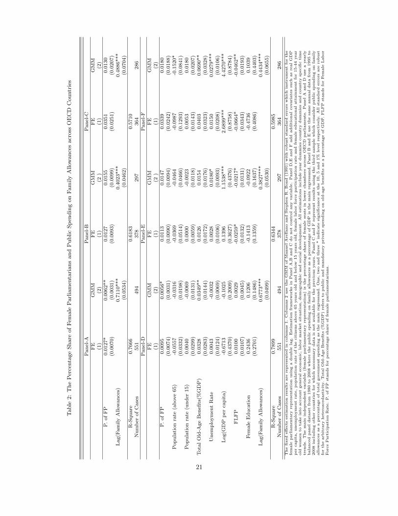
Table 2 shows the estimation results on the relationship between percentage share of female parliamentar-
ians and public spending on family allowances based on three different samples. The estimation frameworks
in Panel A and Panel D use the base sample which is a panel data at one-year intervals for 19 countries be-
10
tween 1980 and 2008. Panel B and Panel E show some estimation results based on the second sample where
the main regressand is public family allowances (as a percentage of GDP). Panel C and Panel F use the third
sample where the main regressand is public family allowances as a percentage of total public spending. Using
these three samples respectively, Panel A, Panel B and Panel C represent results on the relationship between
family allowances and the fraction of female parliamentarians without adding any control variables. Panel
D, Panel E and Panel F add control variables. Considering the econometric specifications without control
variables, the coefficients for the fraction of female parliamentarians are significant in pooled-OLS12 , FE and
GMM estimations. However, using the second and the third samples, the coefficient of the fraction of female
parliamentarians is not significant anymore with the FE and GMM estimations in Panel B and Panel C.
Namely, the relevant results are not robust to estimations when the same techniques are used in the second
and the third samples. Similar finding appears once control variables are added. GMM estimation in Panel
D gives a significant coefficient estimate for the fraction of female parliamentarians. However using neither
FE nor GMM, the coefficient of the fraction of female parliamentarians is not significant using second and
the third samples (Panel E and Panel F). It is an interesting finding that the positive association between
female political participation and public family allowances is found using only the first sample that covers
traditional OECD countries. In contrast to neo-OECD countries, traditional OECD countries have for long
had more numbers of female parliamentarians and results show that their high level participation to politics
may have been translated into larger amount of family allowances compare to neo-OECD countries.
This finding raises a doubt on the fact that the contribution of female parliamentarians to an increase in
family allowances may occur only when their percentage share in parliaments exceed a remarkable value or a
critical mass threshold. Therefore, the paper empirically discusses on the critical mass threshold argument.In
fact, it is possible that the roles of women start to be relevant in terms of bargaining power only when the
percentage share of female parliamentarians reaches a given threshold.
4.2 Relationship Between Female Critical Mass in Parliaments and Public Spend-
ing on Family Allowances
The research on the influence of the critical mass of women relies primarily on Kanter (1977)’s foundational
study. She has hypothesized that women would not be able show their influence in a male-dominated corpo-
rate enviornment, where men (dominants) constitute more than 85 percent and women (tokens) constitute
less than 15 percent of total, since they are subject to performance pressures, role entrapment and boundary
12Due to the biased estimates of Pooled-OLS, relevant findings found using this method is not reported on the tables.
11
heightining. Although her work is the earliest source often cited on the topic and did not deduce a critical
mass threshold for a political enviornment, some political scientists have attempted to determine a critical
mass threshold at which elected female politicians can start to have influence on public spending decisions.
However, the determination of a critical mass threshold is still problematic and undertheorized in the lit-
erature. Related literature can not answer whether there is a single threshold which would be universially
applied. In the literature, threshold has been variously identified at different levels such as 15, 20, 25 or 30
percent (Beckwith and Cowell-Meyers, 2007; Studlar and McAllister, 2002).
Drawing on previous studies, I identify four different thresholds equal to 15, 20, 25 and 30 per cent of
women over total parliamentary seats. Afterwards I test them to examine whether there exists a unique
threshold at which the number of women translates into more public spending on family allowances. Re-
placing main independent variable with thit in equation (1), the role of female critical mass in parliamentary
participation on public family allowances is analyzed using equation (2). In other words, each threshold is
considered as the main independent variable that is a dummy taking value equal to 1 when the share of
female seats exceeds the threshold itself. The rest of the model specification such as the inclusion of control
variables is identical with the equation (1).
yit = αthit + xitβ + γi + µt + υit (2)
Overall findings show that a positive relationship between the fraction of female parliamentarians and public
spending on family allowances exists only when the highest threshold is passed (30%). However, the use of
an arbitrarily chosen critical mass thresholds (15%,20%,25% and 30%) does not mean the analysis is based
on a satisfactory formal test. Therefore, I additionally consider performing a structural break analysis with
an unknown threshold level to formally test for the critical mass argument. Results of the structural break
analysis also supports the evidence on the significance of over 30 per cent participation and more detailed
explanation for this analysis can be found in appendix section.
Turning into results related to thresholds, pooled-OLS estimations on the relationship between the 30%
critical mass threshold and public spending on family allowances give mixed results based on the three
different samples used. However, once country fixed effects are introduced to capture any time-invariant
country characteristics, the positive relationship between the female political representation over 30% critical
mass threshold and the public spending on family allowances holds irrespective of any sample used. The
estimates of α are 0.2324, 0.16 and 0.3236 with the standard errors 0.066, 0.0255, 0.0831 for the first,
12
second and third samples respectively. They are significant at the one percent level where all the standard
errors are robust to arbitrary heteroscedasticity. Moreover, the result on the positive significant relationship
with the fixed effect estimation technique is robust to the inclusion of other additional covariates. As seen
in columns (4) of Table 3, the inclusion of control variables do not change the general finding on the the
positive relationship between over 30 per cent female political participation and the public spending on family
allowances. As an extension to these control variables, columns (5) include two more variables which are
the female labor force participation rate and the female educational attainment. The fixed effect estimates
of α remain significantly positive in this case as well. Findings on the positive significance is also robust to
any sample and the controls that are used under GMM estimation framework. Irrespective of using different
samples at Panel A, B or C, results on the positive relationship are strongly valid under PCSE method as
well. Additionally, all regression estimation techniques in Table 3 use country specific time trends.
As expected, lagged values of the family allowances are positively and strongly related to the public
spending on family allowances in all of the specifications. Turning to other control variables, estimations
based on the first and the third sample show that public and mandatory private spending on old-age benefits
is significant in the specifications of both GMM and PCSE but this result is not robust to estimations based on
the second sample. The log value of GDP per capita is positively significant in all regression estimations of the
third sample (Panel C in Table 3) where the main outcome of interest is public spending on family allowances
as a percentage of total government spending. However, estimations based on the first and the second sample
give mixed results for the significance of GDP. Female labor market participation has a negative relationship
with public spending on family allowances as a percentage of total government expenditures once the second
and third sample are used for the estimations. Women’s earnings may be considered as an additional income
which families rely on. Increasing number of women in labor market increase the income level of households
which causes a decrease in family allowances allocated to households with respect to their new income level.
Some coefficients of the unemployment rate also give expectedly positive signs with GMM estimations when
the third sample is used for the estimations. One possible interpretation for this result could be that family
allowances is a good practice in anti-poverty family policies which are designed to support unemployed
parents for the costs of raising children.
Overall results support (Dahlerup, 1988)’s argument on the critical mass issue. It states that “The idea
of a critical mass is most often applied to situations when women constitute less than 30 percent, in this way
explaining why the entrance of women into politics has not made more difference yet!”. The positive cross-
sectional relationship between the fraction of female parliamentarians and family allowances exists when a
13
certain threshold (30%) is passed. Correspondingly, UN CEDAW’s (The Committee on the Elimination of
Discrimination against Women) General Recommendation on Article 7 of the Convention have also agreed
on the fact that 30 percent is the figure for the female political participation for having a real impact on the
content of policy decisions (CEDAW 1997, paragraph.16). Results in this paper are highly robust to different
econometric techniques from fixed effects to GMM estimation, to estimations in various different samples
and to the inclusion of different sets of covariates although paper does not claim any causal relationship
between related variables due to possible endogeneity problem13.
Moreover, I have not found any significant effect for the other dummy variables associated to the lower
thresholds such as 15%, 20%, 25% (Table 4-6). All the critical mass thresholds under 30% critical mass
threshold show a significant coefficient estimates while using only the pooled OLS estimation technique.
Once country dummies are included to get rid of the bias, the significance disappears. In line with the
previous results of the 15% critical mass threshold, the fraction of female parliamentarians over the 20% or
the 25% critical mass thresholds are also positively significant in the the pooled-OLS estimation framework
based on three different samples. However, these results are not robust to inclusion of country fixed effects,
additional covariates or to the use of different samples. Namely, there is no robust positive relationship
between any critical mass threshold level under the 30% female political representation and the public
spending on family allowances.
5 Empirical Robustness
Robustness of main results are checked in several ways. First of all, the influence of more female parliamen-
tarians on family allowances in the same year when they are just elected can appear unrealistic due to the
yearly time structure of the datasets. In other words, relevant policies can take some time to implement. As
a robustness check for this issue, all estimates are replicated using datasets at 2-year and 3-year intervals to
see the influence of lagged female participation on current family allowances. The main results on the posi-
tive significance of the 30% critical mass threshold remain unchanged using three different samples as seen
in Table 7. I present replications using only the datasets at 3-year intervals. Although it is not presented,
the same also holds using datasets at 2-year intervals. However it is important to emphasize that increasing
13It is known that removing remaining concerns about endogeneity of the female political participation variable wouldnecessitate estimations with instrumental variables. A valid instrumental variable should causally influence female politicalparticipation variable and not be correlated with public spending on family allowances. I believe that such a variable does notexist as it is not used in similar studies that cover gender, public spending and human development issues due to the natureof these variables(Potrafke and Ursprung, 2012; Fortin, 2005; Erhel and Guergoat-Lariviere, 2013; Ruhm, 2000; Tanaka, 2005;Kittilson, 2008).
14
number of intervals unfortunately reduce the number of observations in the datasets. Therefore, due to the
insufficient number of observations, GMM and PCSE techniques can not be applied in contrast to the case
of one year interval.
Secondly, the robustness of the main results are tested adding new variables to see whether more females
have still influencial power on the allocation of expenditures. Each panel of Table 8 investigates the influence
of different covariates on the relationship between the 30% critical mass threshold and the public spending on
family allowances. Panel A adds electoral fractionalization of the party-system. Electoral fractionalization
shows the degree to which political parties in a parliament share the votes in a more equitable way14. In most
of the countries in the world, two big main parties usually share the votes after an election. Liphart (1977)
and Mueller and Murrell (1986) pointed out that the larger number of political parties in a parliament might
decrease efficiency of public spending since multiparty parliaments might make more promises to different
interest groups which can be resulted with less effective reallocation of public expenditures. Econometric
specifications at Panel A of Table 8 control for the electoral fractionalization to check the robustness of
the positive relationship between the 30% critical mass threshold and public spending on family allowances.
All results support the positive significance of it after controlling for the electoral fractionalization as well.
Electoral fractionalization itself has a positive sign only in the PCSE estimations which are done based on
the second and the third samples. However both results are not robust to using GMM and FE techniques.
Therefore it is difficult to make an interpretation on the relationship between the electoral fractionalization
and public spending on family allowances. Furthermore, Panel B includes legislative fractionalization of
the party-system as an other robustness check variable15. Legislative fractionalization is defined as ”the
probability that any two members of the parliament picked at random from the legislature will be from
different parties. This is a measure of the division within parliament which has substantial influence over the
budget”. A higher legislative fractionalization indicates a larger number of small parties occupying legislative
seats. The public finance literature has recently discussed that legislative fractionalization might affect the
level of public spending. Persson and Tabellini (2004) indicate that since majoritarian parliamentary systems
are more likely to produce single party majority governments, whereas coalition and minority governments
become more likely under proportional elections, majoritarian elections lead to smaller welfare programs than
proportional elections. Similarly Roubini and Sachs (1989) explain the higher amount of public spending
14Index of electoral fractionalization of the party-system according to the formula (1−m∑i=1
(vi)2 where vi is the share of votes
for party i and m is the number of parties) proposed by Rae (1968).
15Index of legislative fractionalization of the party-system according to the formula (1−m∑i=1
(si)2 where si is the share of seats
for party i and m is the number of parties) proposed by Rae (1968).
15
with high level of legislative fractionalization and show the presence of many political parties in a ruling
coalition as the reason of larger budget deficits. On the other hand, Bawn and Rosenbluth (2006) find no
effect of a greater number of parties in the legislature on public spending. In line, Volkerink and De Haan
(2001) and Perotti and Kontopoulos (2002) also find some effects that are only marginally significant or not
robust to different estimation frameworks. In this paper, legislative fractionalization itself does not show any
significant relevance on public family allowances. On the other hand, controlling legislative fractionalization
does not change the positive significance of the 30% critical mass threshold.
As another robustness check, the role of female parliamentarians on family allowances is tested regarding
different parliamentary systems. Parliamentary systems are characterized with the presence of either a
majority or a hung (coalition) parliament and larger coalitions tend to be associated with more expenditures,
particularly on transfers (Kontopoulos and Perotti, 1999) since they allow the representation of several
interest groups with respect to gender, race, ethnicity etc. Therefore, the role of over 30 per cent female
parliamentarians on family allowances is tested using two different sub-datasets, which are subset of solely
majority governments and subset of coalition governments. Relevant results are shown in Table 9. As a
surprising result, findings support that female parliamentarians under majority governments might not be
effective in policy making in favor of women when electoral incentives are powerful (see the results at Panel
B in Table 9). Electoral incentives would sometimes make parliamentarians to implement a policy bundle
which is solely favored by the majority of voters, not by her own interest groups. Instead, coefficients belong
to the 30 per cent threshold in coalition governments are significant showing the power of more women
in the allocation of family allowances. However, as expected, if government types (majority or coalition)
are controlled, main results of the paper remained unchanged as seen at Panel C in Tabel 9. All results
represented in this table are obtained using the base sample however they are robust to using second and
the third samples as well.
Moreover, previous literature suggest that the ideology of a governing party can determine the size of
public expenditures and it is argued that left-wing governments expand social transfers more than right-wing
governments. Therefore, composition of the government on the right-left political spectrum is controlled using
”cabinet composition” variable which takes 1 if there is hegemony of right-wing parties, takes 2 if there is
dominance of right wing parties, takes 3, 4 and 5 when there is balance of of power between right and left,
dominance of social democrats together with other left parties and hegemony of social democrats together
with other left parties respectively. However, controlling for cabinet composition does not create any change
in the main results. As another variable, percentage of seats occupied solely by the left-wing parties is
16
controlled but the previous results on the significance of 30 per cent threshold remained unchaged as seen in
Table 10. All results represented in this table are obtained using the base sample however they are robust
to using second and the third samples as well.
6 Conclusions
Representative democracy and the good governance approaches suggest that the participation of the citizens
from different groups in policy making is essential for the fair redistribution. Different voices in public policy
making leads to a resource allocation concerning the preferences of all citizens irrespective of gender, class
and race. Due to the persistent gap between women and men in the political arena, especially female voices
in policy-making has emerged as a global issue all over the world.
The under-representation of women in politics still persist even in the most advanced OECD countries.
Women have constituted just 26.8% percent of the members of parliaments across the OECD in 2012, up
from 19.9% in 2009. There is no country which has reached to equal participation of women and men in
politics among the OECD. Sweden is the only country where male and female parliamentarians have nearly
equal participation with 44.7% of female seats in the parliament. Moreover, the percentage share of the
female seats are still less than one-third in 23 out of 34 OECD countries.
Correspondingly, the percentage share of some public spending categories which reflects women’s prefer-
ences are much more lower than the other spending categories (OECD, 2013). Previous literature suggest
that women are more likely than man to support policies on children and family (Besley and Case, 2000;
Case and Deaton, 1998; Alesina and La Ferrara, 2005; Thomas, 1990; Duflo, 2003; Edlund and Pande, 2002;
Chattopadhyay and Duflo, 2004). Public spending on family allowances is one of the important policies
target especially families who have financial needs for the schooling and the health controls of the children.
Therefore, this paper analyzes whether female under-representation over the thirty years across the OECD
parliaments matters for the low level distribution towards public family allowances. Public spending on
family allowances is a novel contribution which has not been studied before in the relevant literature. My
preference in this subject has also been influenced by the availability of the dataset on family allowances
drawn many new OECD countries that have recently joined the OECD to control the cross-country hetero-
geneity. In fact, estimations based on the data that only includes traditional OECD countries, which have
for long had higher number of female parliamentarians than the new OECD countries, show different results.
To sum up, this paper substantially improves our understanding on the role of female voice. In particular,
17
it helps to explain an important result that small raises in the number of elected female parliamentarians
across the OECD over thirty years might not be enough to observe policy changes in public family allowances,
which probably require stronger changes in female political participation. Using data from the OECD
countries that covers the period of 1980-2010, it is found that female parliamentarians are effective on
increasing the amount of public spending on family allowances once they peaked at a certain critical mass
threshold unless they do not belong to majoritarian governments. This result suggests that the persistent
under-representation of women in the OECD parliaments or their electoral incentives might still be an
obstacle for their efficiency in policy decision making on public family allowances.
7 Appendix
Among papers in the relevant literature, Andrews (1993) initially proposed the following test.
yt = x′tβ1 + εt for t = 1, ......, τ (3)
yt = x′tβ2 + εt for t = τ + 1, ......, T (4)
β1, β2 and xt are at k×1 dimension. There is a single breakpoint, which is τ . Assume the x’s are stationary
and weakly exogenous and the ε’s are serially uncorrelated and homoscedastic. Then we examine the following
hypothesis;
H0 : β1 = β2 (5)
If τ is known the F-statistic is:
FT (τ) = (T − 2k)[SSR1:T − (SSR1:τ + SSRτ+1:T )]/(SSR1:τ + SSRτ+1:T ) (6)
where T is the number of years, k the number of regressors, SSR1:T is the sum of squared residuals of
regression (3) and similarly SSRτ+1:T is the sum of squared residuals of regression (4). The F-statistic
follows asymptotically χ2(k) under H0. In the case where τ is unknown, Quandt (1960) showed that the
18
likelihood ratio statistic corresponding to H0 : β1 = β2 is;
QLRT = maxτε{τmin,......,τmax}
FT (τ) (7)
Andrews (1993) showed that under appropriate regularity conditions, the QLRT statistic, also referred
to as a SupLR statistic has a nonstandard limiting distribution and specifically under H0 is;
QLRT−→D
sup
rε[rmin, rmax](Bk(r)′Bk(r)
r(1− r)) (8)
where 0 < rmin < rmax < 1 and Bk(.) is a Brownian Bridge process defined on [0, 1] and sup is the least
upper bound of a set S.
Accordingly, in Table (11)16 the QLR test statistic, along with the p-values, is reported. It becomes
obvious that every country is exposed in different year of structural break. Then the following regression for
various thresholds is estimated.
yit = αthit + η′i∑i=1
Dit + δ′i∑i=1
Dit × thit + xitβ + γi + µt + υit (9)
where yit is the family allowances, thit indicates the threshold level, Dit is the dummy for country i and
time t, taking value 1 for the post-period (after the structural break) and 0 for the pre-period for i = 1, ......, i
countries. Thus, the regressions control for the dummy Dit, and the interaction term of Dit × thit for all
countries. In Table 12, the coefficient of the threshold (α) for every threshold as well as the F-statistic for
the interaction term Dit × thit are reported. In all cases the null hypothesis of the non-significance of the
joint interaction term Dit× thit for all countries is rejected, confirming that the year of the structural breaks
found in Table 12 exist. On the other hand, the threshold coefficient is significant for a percentage up to
28, while it becomes significant for 29 per cent and higher that almost supports the final finding, which
is 30 per cent, of the paper. The insufficient number of observations did not allow me to test over 33 per
cent, since out of all OECD countries there are only four countries where the percentage share of female
parliamentarians pass 33 per cent as seen in Table 13.
16Due to the longest time dimension compared to other two samples, structural breaks using the first sample of the paperwhich is covered from 1980 to 2008, are shown here. Other structural break tables can be obtained using other samples as well.
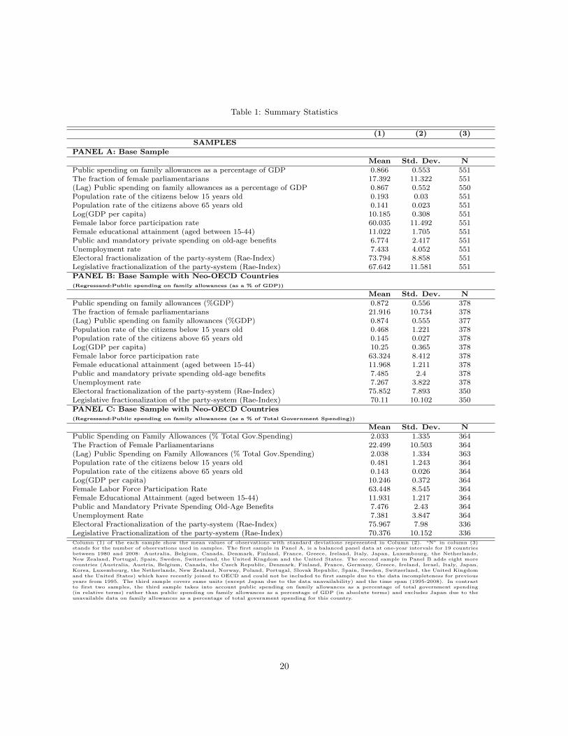
Table 1: Summary Statistics
(1) (2) (3)SAMPLES
PANEL A: Base SampleMean Std. Dev. N
Public spending on family allowances as a percentage of GDP 0.866 0.553 551The fraction of female parliamentarians 17.392 11.322 551(Lag) Public spending on family allowances as a percentage of GDP 0.867 0.552 550Population rate of the citizens below 15 years old 0.193 0.03 551Population rate of the citizens above 65 years old 0.141 0.023 551Log(GDP per capita) 10.185 0.308 551Female labor force participation rate 60.035 11.492 551Female educational attainment (aged between 15-44) 11.022 1.705 551Public and mandatory private spending on old-age benefits 6.774 2.417 551Unemployment rate 7.433 4.052 551Electoral fractionalization of the party-system (Rae-Index) 73.794 8.858 551Legislative fractionalization of the party-system (Rae-Index) 67.642 11.581 551PANEL B: Base Sample with Neo-OECD Countries(Regressand:Public spending on family allowances (as a % of GDP))
Mean Std. Dev. NPublic spending on family allowances (%GDP) 0.872 0.556 378The fraction of female parliamentarians 21.916 10.734 378(Lag) Public spending on family allowances (%GDP) 0.874 0.555 377Population rate of the citizens below 15 years old 0.468 1.221 378Population rate of the citizens above 65 years old 0.145 0.027 378Log(GDP per capita) 10.25 0.365 378Female labor force participation rate 63.324 8.412 378Female educational attainment (aged between 15-44) 11.968 1.211 378Public and mandatory private spending old-age benefits 7.485 2.4 378Unemployment rate 7.267 3.822 378Electoral fractionalization of the party-system (Rae-Index) 75.852 7.893 350Legislative fractionalization of the party-system (Rae-Index) 70.11 10.102 350PANEL C: Base Sample with Neo-OECD Countries(Regressand:Public spending on family allowances (as a % of Total Government Spending))
Mean Std. Dev. NPublic Spending on Family Allowances (% Total Gov.Spending) 2.033 1.335 364The Fraction of Female Parliamentarians 22.499 10.503 364(Lag) Public Spending on Family Allowances (% Total Gov.Spending) 2.038 1.334 363Population rate of the citizens below 15 years old 0.481 1.243 364Population rate of the citizens above 65 years old 0.143 0.026 364Log(GDP per capita) 10.246 0.372 364Female Labor Force Participation Rate 63.448 8.545 364Female Educational Attainment (aged between 15-44) 11.931 1.217 364Public and Mandatory Private Spending Old-Age Benefits 7.476 2.43 364Unemployment Rate 7.381 3.847 364Electoral Fractionalization of the party-system (Rae-Index) 75.967 7.98 336Legislative Fractionalization of the party-system (Rae-Index) 70.376 10.152 336Column (1) of the each sample show the mean values of observations with standard deviations represented in Column (2). “N” in column (3)stands for the number of observations used in samples. The first sample in Panel A, is a balanced panel data at one-year intervals for 19 countriesbetween 1980 and 2008: Australia, Belgium, Canada, Denmark, Finland, France, Greece, Ireland, Italy, Japan, Luxembourg, the Netherlands,New Zealand, Portugal, Spain, Sweden, Switzerland, the United Kingdom and the United States. The second sample in Panel B adds eight morecountries (Australia, Austria, Belgium, Canada, the Czech Republic, Denmark, Finland, France, Germany, Greece, Ireland, Israel, Italy, Japan,Korea, Luxembourg, the Netherlands, New Zealand, Norway, Poland, Portugal, Slovak Republic, Spain, Sweden, Switzerland, the United Kingdomand the United States) which have recently joined to OECD and could not be included to first sample due to the data incompleteness for previousyears from 1995. The third sample covers same units (except Japan due to the data unavailability) and the time span (1995-2008). In contrastto first two samples, the third sample takes into account public spending on family allowances as a percentage of total government spending(in relative terms) rather than public spending on family allowances as a percentage of GDP (in absolute terms) and excludes Japan due to theunavailable data on family allowances as a percentage of total government spending for this country.
20
Table
2:
The
Per
centa
ge
Share
of
Fem
ale
Parl
iam
enta
rians
and
Public
Sp
endin
gon
Fam
ily
Allow
ance
sacr
oss
OE
CD
Countr
ies
Pan
el-A
Pan
el-B
Pan
el-C
FE
GM
MF
EG
MM
FE
GM
M(1
)(2
)(1
)(2
)(1
)(2
)P
.of
FP
0.0
127*
0.0
062**
0.0
127
0.0
155
0.0
351
0.0
130
(0.0
070)
(0.0
031)
(0.0
093)
(0.0
099)
(0.0
251)
(0.0
207)
Lag(F
am
ily
Allow
ance
s)0.7
110***
0.4
023***
0.4
886***
(0.0
534)
(0.0
462)
(0.0
704)
R-S
qu
are
0.7
666
0.6
183
0.5
710
Nu
mb
erof
Case
s551
494
378
297
364
286
Pan
el-D
Pan
el-E
Pan
el-F
FE
GM
MF
EG
MM
FE
GM
M(1
)(2
)(1
)(2
)(1
)(2
)P
.of
FP
0.0
095
0.0
056*
0.0
113
0.0
147
0.0
339
0.0
180
(0.0
074)
(0.0
031)
(0.0
090)
(0.0
094)
(0.0
242)
(0.0
188)
Pop
ula
tion
rate
(ab
ove
65)
-0.0
557
-0.0
316
-0.0
369
-0.0
464
-0.0
987
-0.1
520*
(0.0
332)
(0.0
198)
(0.0
514)
(0.0
466)
(0.1
293)
(0.0
841)
Pop
ula
tion
rate
(un
der
15)
0.0
040
-0.0
069
0.0
000
-0.0
023
0.0
053
0.0
180
(0.0
299)
(0.0
131)
(0.0
059)
(0.0
118)
(0.0
143)
(0.0
207)
Tota
lO
ld-A
ge
Ben
efits
(%G
DP
)0.0
328
0.0
349**
0.0
126
0.0
154
0.0
403
0.0
690**
(0.0
283)
(0.0
144)
(0.0
172)
(0.0
176)
(0.0
323)
(0.0
328)
Un
emp
loym
ent
Rate
0.0
043
-0.0
032
0.0
028
0.0
180*
0.0
150
0.0
279***
(0.0
124)
(0.0
069)
(0.0
106)
(0.0
093)
(0.0
208)
(0.0
106)
Log(G
DP
per
cap
ita)
-0.6
713
-0.1
025
0.1
396
1.1
538***
2.6
899***
4.4
270***
(0.4
370)
(0.2
009)
(0.3
627)
(0.4
376)
(0.8
758)
(0.8
784)
FL
FP
0.0
100
0.0
029
-0.0
259*
-0.0
217*
-0.0
664*
-0.0
462**
(0.0
107)
(0.0
045)
(0.0
132)
(0.0
131)
(0.0
343)
(0.0
193)
Fem
ale
Ed
uca
tion
0.2
436
0.1
206
-0.1
413
-0.0
922
-0.4
736
0.1
039
(0.2
701)
(0.1
486)
(0.1
359)
(0.1
637)
(0.4
086)
(0.4
403)
Lag(F
am
ily
Allow
ance
s)0.6
773***
0.3
827***
0.4
434***
(0.0
499)
(0.0
530)
(0.0
655)
R-S
qu
are
0.7
899
0.6
344
0.5
985
Nu
mb
erof
Case
s551
494
378
297
364
286
The
fixed
eff
ects
est
imati
on
resu
lts
are
repre
sente
din
colu
mns
1.
Colu
mns
2use
the
GM
Mof
Manuel
Are
llano
and
Ste
phen
R.
Bond
(1991)
wit
hro
bust
standard
err
ors
whic
hin
stru
ment
for
the
fem
ale
parl
iam
enta
ryre
pre
senta
tion
usi
ng
adouble
lag.
Est
imati
on
fram
ew
ork
sin
Panel
A,B
and
Cdo
not
contr
ol
any
vari
able
.P
anel
D,E
and
Fadd
addit
ional
covari
ate
ssu
ch
as
real
GD
Pp
er
capit
a,
unem
plo
ym
ent
rate
,p
opula
tion
rate
of
the
cit
izens
ab
ove
65
years
old
and
belo
w15
years
old
,fe
male
lab
or
forc
epart
icip
ati
on
rate
and
fem
ale
educati
onal
att
ain
ment
for
15-4
4year
old
wom
en
tota
ke
into
account
genera
leconom
ic,
lab
or
mark
et
situ
ati
on,
dem
ogra
phic
and
socia
ldevelo
pm
ent.
All
est
imati
ons
inclu
de
year
dum
mie
scountr
ydum
mie
sand
countr
ysp
ecifi
cti
me
trends.
The
main
indep
endent
vari
able
(fem
ale
parl
iam
enta
ryre
pre
senta
tion)
isth
ep
erc
enta
ge
share
of
fem
ale
seats
inlo
wer
cham
bers
acro
ssO
EC
Dparl
iam
ents
.P
anel
Aand
Duse
ayearl
ybala
nced
panel
data
set
from
1980
to2008
where
the
public
spendin
gon
fam
ily
allow
ances
as
ap
erc
enta
ge
of
GD
Pis
the
main
regre
ssand.
Panel
Band
Euse
the
sam
eannual
data
from
1995
to2008
inclu
din
goth
er
countr
ies
for
whic
hnecess
sary
data
isnot
available
for
the
pre
vio
us
years
.P
anel
Cand
Fre
pre
sent
resu
lts
usi
ng
the
thir
dsa
mple
whic
hconsi
der
public
spendin
gon
fam
ily
allow
ances
as
ap
erc
enta
ge
of
tota
lgovenm
ent
spendin
gas
the
main
regre
ssand.
One,
two
and
thre
e*
indic
ate
signifi
cance
at
the
10,
5and
1%
level
resp
ecti
vely
.A
llst
andard
err
ors
are
robust
for
the
arb
itra
ryhete
rosc
edast
icit
y.
Tota
lO
ld-A
ge
Benefi
ts(%
GD
P)
refe
rsto
public
and
mandato
rypri
vate
spendin
gon
old
-age
benefi
tsas
ap
erc
enta
ge
of
GD
P.
FL
FP
stands
for
Fem
ale
Lab
or
Forc
eP
art
icip
ati
on
Rate
.P
.of
FP
stands
for
perc
enta
ge
share
of
fem
ale
parl
iam
enta
rians.
21

Table
3:
Fem
ale
Politi
cal
Rep
rese
nta
tion
over
the
30%
Fem
ale
Cri
tica
lM
ass
Thre
shold
and
Public
Sp
endin
gon
Fam
ily
Allow
ance
s
FE
GM
MP
CSE
FE
FE
GM
MG
MM
PC
SE
(1)
(2)
(3)
(4)
(5)
(6)
(7)
(8)
PA
NE
LA
Thre
shold
-30
thre
sh30
0.2
324***
0.0
938**
0.1
557***
0.2
342***
0.2
202***
0.0
914***
0.0
878***
0.1
466***
(0.0
666)
(0.0
369)
(0.0
344)
(0.0
639)
(0.0
649)
(0.0
325)
(0.0
326)
(0.0
326)
Lag(F
am
ily
All
ow
ances)
0.6
951***
0.3
042***
0.6
597***
0.6
570***
0.2
735***
(0.0
483)
(0.0
416)
(0.0
451)
(0.0
416)
(0.0
394)
Popula
tion
rate
(ab
ove
65)
-0.0
291
-0.0
336
-0.0
240
-0.0
231
-0.0
244
(0.0
354)
(0.0
324)
(0.0
195)
(0.0
183)
(0.0
184)
Popula
tion
rate
(under
15)
0.0
078
0.0
062
-0.0
056
-0.0
057
0.0
091
(0.0
238)
(0.0
252)
(0.0
114)
(0.0
115)
(0.0
099)
Tota
lO
ld-A
ge
Benefi
ts(%
GD
P)
0.0
324
0.0
308
0.0
351***
0.0
346**
0.0
285**
(0.0
256)
(0.0
276)
(0.0
123)
(0.0
138)
(0.0
128)
Unem
plo
ym
ent
Rate
0.0
086
0.0
077
-0.0
024
-0.0
030
0.0
041
(0.0
123)
(0.0
117)
(0.0
066)
(0.0
063)
(0.0
040)
Log(G
DP
per
capit
a)
-0.5
268
-0.5
689
-0.1
239
-0.1
321
-0.3
079*
(0.3
774)
(0.4
006)
(0.2
028)
(0.1
876)
(0.1
728)
FL
FP
0.0
035
0.0
014
0.0
043
(0.0
096)
(0.0
042)
(0.0
046)
Fem
ale
educati
on
0.1
881
0.1
277
0.1
345
(0.2
494)
(0.1
449)
(0.1
042)
R-S
quare
0.7
778
0.9
452
0.7
999
0.8
010
0.9
471
Num
ber
of
Case
s551
494
550
551
551
494
494
550
PA
NE
LB
Thre
shold
-30
0.1
600***
0.1
660***
0.1
298***
0.1
594***
0.1
589***
0.1
401***
0.1
399***
0.1
223**
(0.0
255)
(0.0
358)
(0.0
446)
(0.0
361)
(0.0
310)
(0.0
396)
(0.0
401)
(0.0
504)
Lag(F
am
ily
All
ow
ances)
0.4
018***
0.1
495***
0.4
153***
0.3
919***
0.1
510***
(0.0
257)
(0.0
527)
(0.0
230)
(0.0
309)
(0.0
506)
Popula
tion
rate
(ab
ove
65)
0.0
020
-0.0
078
-0.0
517
-0.0
479
-0.0
142
(0.0
526)
(0.0
473)
(0.0
394)
(0.0
349)
(0.0
241)
Popula
tion
rate
(under
15)
0.0
011
0.0
044
0.0
081
0.0
091
0.0
013
(0.0
052)
(0.0
059)
(0.0
115)
(0.0
111)
(0.0
044)
Tota
lO
ld-A
ge
Benefi
ts(%
GD
P)
0.0
217
0.0
154
0.0
277
0.0
221
0.0
181*
(0.0
205)
(0.0
190)
(0.0
188)
(0.0
199)
(0.0
095)
Unem
plo
ym
ent
Rate
-0.0
051
-0.0
000
0.0
103
0.0
132**
0.0
014
(0.0
125)
(0.0
107)
(0.0
067)
(0.0
063)
(0.0
051)
Log(G
DP
per
capit
a)
-0.1
656
0.0
898
0.9
990***
1.0
698***
0.2
562
(0.2
518)
(0.2
744)
(0.3
625)
(0.3
488)
(0.3
064)
FL
FP
-0.0
273*
-0.0
163
-0.0
216***
(0.0
139)
(0.0
126)
(0.0
062)
Fem
ale
educati
on
-0.1
419
-0.0
217
-0.1
278
(0.1
411)
(0.1
670)
(0.1
790)
R-S
quare
0.6
189
0.9
688
0.6
224
0.6
357
0.9
702
Num
ber
of
Case
s378
297
377
378
378
297
297
377
PA
NE
LC
Thre
shold
-30
0.3
236***
0.2
741**
0.2
407**
0.3
498***
0.3
453***
0.3
126*
0.3
190*
0.2
459**
(0.0
831)
(0.1
345)
(0.0
956)
(0.1
220)
(0.1
100)
(0.1
613)
(0.1
635)
(0.1
100)
Lag(F
am
ily
All
ow
ances)
0.4
742***
0.0
985**
0.4
523***
0.4
321***
0.1
158***
(0.0
542)
(0.0
462)
(0.0
440)
(0.0
385)
(0.0
435)
Popula
tion
rate
(ab
ove
65)
-0.0
190
-0.0
432
-0.1
207
-0.1
099
-0.0
593
(0.1
224)
(0.1
215)
(0.0
816)
(0.0
743)
(0.0
532)
Popula
tion
rate
(under
15)
0.0
060
0.0
144
0.0
409
0.0
424
0.0
069
(0.0
118)
(0.0
142)
(0.0
279)
(0.0
269)
(0.0
107)
Tota
lO
ld-A
ge
Benefi
ts(%
GD
P)
0.0
643
0.0
483
0.0
805***
0.0
726**
0.0
497**
(0.0
425)
(0.0
388)
(0.0
306)
(0.0
321)
(0.0
242)
Unem
plo
ym
ent
Rate
-0.0
052
0.0
079
0.0
177**
0.0
239**
0.0
134
(0.0
256)
(0.0
219)
(0.0
089)
(0.0
103)
(0.0
142)
Log(G
DP
per
capit
a)
1.8
844**
2.5
017***
4.2
015***
4.4
777***
2.7
556***
(0.7
206)
(0.8
376)
(0.8
918)
(0.9
131)
(0.8
818)
FL
FP
-0.0
703*
-0.0
405*
-0.0
579***
(0.0
376)
(0.0
211)
(0.0
135)
Fem
ale
educati
on
-0.4
974
0.1
634
-0.4
291
(0.4
388)
(0.4
250)
(0.4
168)
R-S
quare
0.5
594
0.9
611
0.5
709
0.5
885
0.9
652
Num
ber
of
Case
s364
286
363
364
364
286
286
363
The
fixed
eff
ects
est
imati
on
resu
lts
are
show
nin
colu
mns
(1),
(4),
(5).
Colu
mns
(2),
(6)
and
(7)
use
the
GM
Mof
Manuel
Are
llano
and
Ste
phen
R.
Bond
(1991)
whic
hin
stru
ment
for
the
30%
fem
ale
parl
iam
enta
ryre
pre
senta
tion
usi
ng
adouble
lag.
To
contr
ol
for
conte
mp
ora
neous
corr
ela
tion,
panel-
corr
ecte
dst
andard
err
ors
are
rep
ort
ed
incolu
mns
(3)
and
colu
mns
(8)
whic
hin
clu
de
auto
regre
ssiv
epro
cess
es
of
ord
er
one
(AR
(1))
.It
indic
ate
sth
epre
sence
of
seri
al
corr
ela
tion
and
allow
ing
Pra
is-W
inst
en
regre
ssio
nfo
rth
ecorr
ecti
on
of
seri
al
corr
ela
tion.
Follow
ing
the
pre
vio
us
lite
ratu
re,
colu
mns
(4)
and
colu
mns
(6)
add
addit
ional
covari
ate
ssu
ch
as
real
GD
Pp
er
capit
a,
unem
plo
ym
ent
rate
,p
opula
tion
rate
of
the
cit
izens
ab
ove
65
years
old
and
belo
w15
years
old
tota
ke
into
account
genera
leconom
icdevelo
pm
ent,
lab
or
mark
et
situ
ati
on
and
dem
ogra
phic
develo
pm
ent.
Inaddit
ion
toth
ese
covari
ate
s,colu
mns
(5),
(7)
and
(8)
add
als
ofe
male
lab
or
forc
epart
icip
ati
on
rate
and
fem
ale
educati
onal
att
ain
ment
for
15-4
4year
old
wom
en
tota
ke
into
account
socia
ldevelo
pm
ent.
Year
dum
mie
sare
inclu
ded
inall
regre
ssio
ns.
More
over,
all
est
imati
ons
inclu
de
countr
ydum
mie
sand
countr
ysp
ecifi
cti
me
trends.
The
main
indep
endent
vari
able
(Thre
shold
-30)
isa
dum
my
vari
able
whic
his
the
pro
xy
for
gender
barg
ain
ing
pow
er.
Itta
kes
avalu
eequal
to1
when
the
share
of
fem
ale
seats
innati
onal
parl
iam
ents
acro
ssO
EC
Dexceed
30%
.P
anel
Ause
sa
yearl
ybala
nced
panel
data
from
1980
to2008
where
the
public
spendin
gon
fam
ily
allow
ances
as
ap
erc
enta
ge
of
GD
Pis
the
main
regre
ssand.
Panel
Buse
sth
esa
me
annual
data
from
1995
to2008
inclu
din
goth
er
countr
ies
for
whic
hth
enecess
sary
data
isnot
available
for
the
pre
vio
us
years
.P
anel
Cuse
sth
esa
me
sam
ple
inP
anel
Bw
here
the
public
spendin
gon
fam
ily
allow
ances
as
ap
erc
enta
ge
of
tota
lgovenm
ent
spendin
gis
the
main
regre
ssand.
One,
two
and
thre
e*
indic
ate
signifi
cance
at
the
10,
5and
1%
level
resp
ecti
vely
.T
ota
lO
ld-A
ge
Benefi
ts(%
GD
P)
refe
rsto
public
and
mandato
rypri
vate
spendin
gon
old
-age
benefi
tsas
ap
erc
enta
ge
of
GD
P.
All
standard
err
ors
are
robust
for
the
arb
itra
ryhete
rosc
edast
icit
y.
FL
FP
stands
for
Fem
ale
Lab
or
Forc
eP
art
icip
ati
on
Rate
.
22

Table
4:
Fem
ale
Politi
cal
Rep
rese
nta
tion
over
the
15%
Fem
ale
Cri
tica
lM
ass
Thre
shold
and
Public
Sp
endin
gon
Fam
ily
Allow
ance
s
FE
GM
MP
CSE
FE
FE
GM
MG
MM
PC
SE
(1)
(2)
(3)
(4)
(5)
(6)
(7)
(8)
PA
NE
LA
Thre
shold
-15
0.0
592
0.0
128
0.0
346
0.0
218
0.0
295
-0.0
009
-0.0
015
0.0
209
(0.0
563)
(0.0
289)
(0.0
220)
(0.0
624)
(0.0
620)
(0.0
272)
(0.0
280)
(0.0
235)
Lag(F
am
ily
All
ow
ances)
0.7
209***
0.3
294***
0.6
902***
0.6
843***
0.3
041***
(0.0
491)
(0.0
409)
(0.0
474)
(0.0
431)
(0.0
390)
Popula
tion
rate
(ab
ove
65)
-0.0
361
-0.0
516
-0.0
305*
-0.0
311*
-0.0
335*
(0.0
386)
(0.0
316)
(0.0
184)
(0.0
172)
(0.0
183)
Popula
tion
rate
(under
15)
0.0
158
0.0
080
-0.0
041
-0.0
054
0.0
110
(0.0
296)
(0.0
313)
(0.0
116)
(0.0
120)
(0.0
101)
Tota
lO
ld-A
ge
Benefi
ts(%
GD
P)
0.0
339
0.0
349
0.0
356***
0.0
362***
0.0
310**
(0.0
262)
(0.0
283)
(0.0
122)
(0.0
133)
(0.0
127)
Unem
plo
ym
ent
rate
0.0
029
0.0
025
-0.0
046
-0.0
051
0.0
010
(0.0
132)
(0.0
121)
(0.0
068)
(0.0
064)
(0.0
041)
Log(G
DP
per
capit
a)
-0.6
272
-0.7
334
-0.1
451
-0.1
724
-0.3
726**
(0.4
289)
(0.4
419)
(0.1
979)
(0.1
810)
(0.1
727)
FL
FP
0.0
122
0.0
035
0.0
094**
(0.0
108)
(0.0
043)
(0.0
047)
Fem
ale
educati
on
0.2
942
0.1
431
0.1
885*
(0.2
627)
(0.1
388)
(0.1
050)
R-S
quare
0.7
591
0.9
432
0.7
803
0.7
854
0.9
467
Num
ber
of
Case
s551
494
550
551
551
494
494
550
PA
NE
LB
Thre
shold
-15
0.0
284
-0.0
678
-0.0
115
0.0
263
0.0
268
-0.0
243
-0.0
163
-0.0
105
(0.0
509)
(0.1
102)
(0.0
213)
(0.0
487)
(0.0
488)
(0.0
973)
(0.0
998)
(0.0
228)
Lag(F
am
ily
All
ow
ances)
0.4
416***
0.1
576***
0.4
502***
0.4
277***
0.1
616***
(0.0
385)
(0.0
531)
(0.0
411)
(0.0
481)
(0.0
509)
Popula
tion
rate
(ab
ove
65)
-0.0
397
-0.0
489
-0.0
850*
-0.0
811*
-0.0
414*
(0.0
559)
(0.0
522)
(0.0
506)
(0.0
443)
(0.0
224)
Popula
tion
rate
(under
15)
-0.0
039
-0.0
006
-0.0
030
-0.0
022
-0.0
025
(0.0
054)
(0.0
061)
(0.0
117)
(0.0
112)
(0.0
041)
Tota
lO
ld-A
ge
Benefi
ts(%
GD
P)
0.0
204
0.0
141
0.0
302
0.0
247
0.0
186*
(0.0
207)
(0.0
192)
(0.0
227)
(0.0
242)
(0.0
099)
Unem
plo
ym
ent
Rate
-0.0
030
0.0
021
0.0
105
0.0
135**
0.0
024
(0.0
126)
(0.0
109)
(0.0
070)
(0.0
069)
(0.0
052)
Log(G
DP
per
capit
a)
-0.1
738
0.0
788
0.8
863**
0.9
648***
0.2
269
(0.2
815)
(0.3
300)
(0.3
689)
(0.3
570)
(0.3
184)
FL
FP
-0.0
271*
-0.0
156
-0.0
210***
(0.0
141)
(0.0
138)
(0.0
064)
Fem
ale
educati
on
-0.1
636
-0.0
285
-0.1
525
(0.1
411)
(0.1
466)
(0.1
879)
R-S
quare
0.6
013
0.9
672
0.6
079
0.6
213
0.9
693
Num
ber
of
Case
s378
297
377
378
378
297
297
377
PA
NE
LC
Thre
shold
-15
0.1
299
-0.4
065
0.0
150
0.1
485
0.1
481
-0.2
864
-0.2
849
0.0
360
(0.1
380)
(0.3
552)
(0.0
491)
(0.1
332)
(0.1
328)
(0.3
510)
(0.3
467)
(0.0
512)
Lag(F
am
ily
All
ow
ances)
0.4
759***
0.0
983**
0.4
639***
0.4
498***
0.1
185***
(0.0
517)
(0.0
467)
(0.0
429)
(0.0
418)
(0.0
440)
Popula
tion
rate
(ab
ove
65)
-0.1
223
-0.1
454
-0.1
893*
-0.1
860*
-0.1
191**
(0.1
182)
(0.1
208)
(0.1
043)
(0.0
981)
(0.0
492)
Popula
tion
rate
(under
15)
-0.0
054
0.0
032
0.0
157
0.0
176
-0.0
005
(0.0
117)
(0.0
142)
(0.0
249)
(0.0
225)
(0.0
103)
Tota
lO
ld-A
ge
Benefi
ts(%
GD
P)
0.0
576
0.0
414
0.0
867**
0.0
801*
0.0
477*
(0.0
404)
(0.0
367)
(0.0
413)
(0.0
429)
(0.0
250)
Unem
plo
ym
ent
Rate
0.0
010
0.0
141
0.0
182*
0.0
238**
0.0
166
(0.0
256)
(0.0
220)
(0.0
103)
(0.0
119)
(0.0
141)
Log(G
DP
per
capit
a)
1.9
516**
2.5
730**
3.7
372***
4.0
139***
2.7
388***
(0.8
120)
(0.9
687)
(0.8
781)
(0.9
421)
(0.8
856)
FL
FP
-0.0
708*
-0.0
364
-0.0
574***
(0.0
376)
(0.0
231)
(0.0
137)
Fem
ale
educati
on
-0.5
109
0.3
085
-0.4
381
(0.4
608)
(0.4
427)
(0.4
312)
R-S
quare
0.5
484
0.9
587
0.5
613
0.5
792
0.9
637
Num
ber
of
Case
s364
286
363
364
364
286
286
363
The
fixed
eff
ects
est
imati
on
resu
lts
are
show
nin
colu
mns
(1),
(4),
(5).
Colu
mns
(2),
(6)
and
(7)
use
the
GM
Mof
Manuel
Are
llano
and
Ste
phen
R.
Bond
(1991)
whic
hin
stru
ment
for
the
15%
fem
ale
parl
iam
enta
ryre
pre
senta
tion
usi
ng
adouble
lag.
To
contr
ol
for
conte
mp
ora
neous
corr
ela
tion,
panel-
corr
ecte
dst
andard
err
ors
are
rep
ort
ed
incolu
mns
(3)
and
colu
mns
(8)
whic
hin
clu
de
auto
regre
ssiv
epro
cess
es
of
ord
er
one
(AR
(1))
.It
indic
ate
sth
epre
sence
of
seri
al
corr
ela
tion
and
allow
ing
Pra
is-W
inst
en
regre
ssio
nfo
rth
ecorr
ecti
on
of
seri
al
corr
ela
tion.
Follow
ing
the
pre
vio
us
lite
ratu
re,
colu
mns
(4)
and
colu
mns
(6)
add
addit
ional
covari
ate
ssu
ch
as
real
GD
Pp
er
capit
a,
unem
plo
ym
ent
rate
,p
opula
tion
rate
of
the
cit
izens
ab
ove
65
years
old
and
belo
w15
years
old
tota
ke
into
account
genera
leconom
icdevelo
pm
ent,
lab
or
mark
et
situ
ati
on
and
dem
ogra
phic
develo
pm
ent.
Inaddit
ion
toth
ese
covari
ate
s,colu
mns
(5),
(7)
and
(8)
add
als
ofe
male
lab
or
forc
epart
icip
ati
on
rate
and
fem
ale
educati
onal
att
ain
ment
for
15-4
4year
old
wom
en
tota
ke
into
account
socia
ldevelo
pm
ent.
Year
dum
mie
sare
inclu
ded
inall
regre
ssio
ns.
More
over,
all
est
imati
ons
inclu
de
countr
ydum
mie
sand
countr
ysp
ecifi
cti
me
trends.
The
main
indep
endent
vari
able
(Thre
shold
-15)
isa
dum
my
vari
able
whic
his
the
pro
xy
for
gender
barg
ain
ing
pow
er.
Itta
kes
avalu
eequal
to1
when
the
share
of
fem
ale
seats
innati
onal
parl
iam
ents
acro
ssO
EC
Dexceed
15%
.P
anel
Ause
sa
yearl
ybala
nced
panel
data
from
1980
to2008
where
the
public
spendin
gon
fam
ily
allow
ances
as
ap
erc
enta
ge
of
GD
Pis
the
main
regre
ssand.
Panel
Buse
sth
esa
me
annual
data
from
1995
to2008
inclu
din
goth
er
countr
ies
for
whic
hth
enecess
sary
data
isnot
available
for
the
pre
vio
us
years
.P
anel
Cuse
sth
esa
me
sam
ple
inP
anel
Bw
here
the
public
spendin
gon
fam
ily
allow
ances
as
ap
erc
enta
ge
of
tota
lgovenm
ent
spendin
gis
the
main
regre
ssand.
One,
two
and
thre
e*
indic
ate
signifi
cance
at
the
10,
5and
1%
level
resp
ecti
vely
.T
ota
lO
ld-A
ge
Benefi
ts(%
GD
P)
refe
rsto
public
and
mandato
rypri
vate
spendin
gon
old
-age
benefi
tsas
ap
erc
enta
ge
of
GD
P.
All
standard
err
ors
are
robust
for
the
arb
itra
ryhete
rosc
edast
icit
y.
FL
FP
stands
for
Fem
ale
Lab
or
Forc
eP
art
icip
ati
on
Rate
.
23
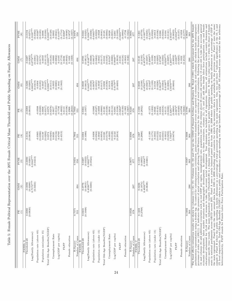
Table
5:
Fem
ale
Politi
cal
Rep
rese
nta
tion
over
the
20%
Fem
ale
Cri
tica
lM
ass
Thre
shold
and
Public
Sp
endin
gon
Fam
ily
Allow
ance
s
FE
GM
MP
CSE
FE
FE
GM
MG
MM
PC
SE
(1)
(2)
(3)
(4)
(5)
(6)
(7)
(8)
PA
NE
LA
Thre
shold
-20
0.0
080
-0.0
090
-0.0
090
-0.0
184
-0.0
089
-0.0
286
-0.0
287
-0.0
194
(0.0
830)
(0.0
289)
(0.0
261)
(0.0
818)
(0.0
819)
(0.0
265)
(0.0
262)
(0.0
271)
Lag(F
am
ily
All
ow
ances)
0.7
173***
0.3
342***
0.6
834***
0.6
778***
0.3
109***
(0.0
453)
(0.0
413)
(0.0
419)
(0.0
381)
(0.0
392)
Popula
tion
rate
(ab
ove
65)
-0.0
365
-0.0
508
-0.0
304
-0.0
310*
-0.0
326*
(0.0
396)
(0.0
329)
(0.0
185)
(0.0
171)
(0.0
185)
Popula
tion
rate
(under
15)
0.0
139
0.0
068
-0.0
047
-0.0
059
0.0
096
(0.0
292)
(0.0
317)
(0.0
107)
(0.0
113)
(0.0
100)
Tota
lO
ld-A
ge
Benefi
ts(%
GD
P)
0.0
374
0.0
379
0.0
390***
0.0
395***
0.0
339***
(0.0
245)
(0.0
278)
(0.0
111)
(0.0
124)
(0.0
129)
Unem
plo
ym
ent
Rate
0.0
020
0.0
017
-0.0
055
-0.0
060
0.0
002
(0.0
134)
(0.0
124)
(0.0
065)
(0.0
062)
(0.0
041)
Log(G
DP
per
capit
a)
-0.6
769
-0.7
736
-0.1
841
-0.2
105
-0.4
105**
(0.4
313)
(0.4
602)
(0.1
843)
(0.1
719)
(0.1
714)
FL
FP
0.0
113
0.0
036
0.0
088*
(0.0
108)
(0.0
043)
(0.0
046)
Fem
ale
educati
on
0.2
966
0.1
422
0.1
872*
(0.2
650)
(0.1
308)
(0.1
057)
R-S
quare
0.7
571
0.9
434
0.7
802
0.7
850
0.9
476
Num
ber
of
Case
s551
494
550
551
551
494
494
550
PA
NE
LB
Thre
shold
-20
0.0
431
0.0
776
0.0
487
0.0
384
0.0
364
0.0
649
0.0
785
0.0
444
(0.1
048)
(0.0
815)
(0.0
332)
(0.1
080)
(0.1
057)
(0.0
812)
(0.0
811)
(0.0
325)
Lag(F
am
ily
All
ow
ances)
0.4
330***
0.1
602***
0.4
445***
0.4
148***
0.1
656***
(0.0
493)
(0.0
524)
(0.0
538)
(0.0
608)
(0.0
506)
Popula
tion
rate
(ab
ove
65)
-0.0
406
-0.0
486
-0.0
876*
-0.0
811*
-0.0
465**
(0.0
564)
(0.0
527)
(0.0
521)
(0.0
464)
(0.0
223)
Popula
tion
rate
(under
15)
-0.0
040
-0.0
008
-0.0
049
-0.0
045
-0.0
028
(0.0
054)
(0.0
060)
(0.0
117)
(0.0
117)
(0.0
041)
Tota
lO
ld-A
ge
Benefi
ts(%
GD
P)
0.0
180
0.0
120
0.0
238
0.0
163
0.0
145
(0.0
179)
(0.0
168)
(0.0
180)
(0.0
185)
(0.0
094)
Unem
plo
ym
ent
Rate
-0.0
033
0.0
016
0.0
119
0.0
154*
0.0
028
(0.0
128)
(0.0
112)
(0.0
082)
(0.0
080)
(0.0
051)
Log(G
DP
per
capit
a)
-0.2
122
0.0
294
0.9
179**
0.9
948**
0.2
261
(0.2
914)
(0.3
108)
(0.4
003)
(0.3
919)
(0.3
169)
FL
FP
-0.0
263*
-0.0
181
-0.0
205***
(0.0
130)
(0.0
124)
(0.0
064)
Fem
ale
educati
on
-0.1
985
-0.0
643
-0.1
738
(0.1
907)
(0.1
646)
(0.1
824)
R-S
quare
0.6
026
0.9
671
0.6
088
0.6
220
0.9
694
Num
ber
of
Case
s378
297
377
378
378
297
297
377
PA
NE
LC
Thre
shold
-20
0.1
403
0.0
236
0.1
219
0.1
367
0.1
339
0.0
049
0.0
145
0.1
261
(0.2
768)
(0.1
874)
(0.0
855)
(0.2
886)
(0.2
832)
(0.2
108)
(0.2
193)
(0.0
779)
Lag(F
am
ily
All
ow
ances)
0.4
932***
0.1
004**
0.4
762***
0.4
579***
0.1
189***
(0.0
638)
(0.0
461)
(0.0
567)
(0.0
597)
(0.0
435)
Popula
tion
rate
(ab
ove
65)
-0.1
189
-0.1
375
-0.2
163*
-0.2
069**
-0.1
247**
(0.1
171)
(0.1
202)
(0.1
109)
(0.1
039)
(0.0
502)
Popula
tion
rate
(under
15)
-0.0
054
0.0
026
0.0
158
0.0
168
-0.0
013
(0.0
122)
(0.0
143)
(0.0
226)
(0.0
205)
(0.0
106)
Tota
lO
ld-A
ge
Benefi
ts(%
GD
P)
0.0
512
0.0
358
0.0
819**
0.0
738*
0.0
386
(0.0
341)
(0.0
318)
(0.0
384)
(0.0
393)
(0.0
244)
Unem
plo
ym
ent
Rate
-0.0
012
0.0
115
0.0
189**
0.0
250***
0.0
164
(0.0
259)
(0.0
226)
(0.0
085)
(0.0
097)
(0.0
141)
Log(G
DP
per
capit
a)
1.7
563**
2.3
281**
3.9
378***
4.2
057***
2.6
533***
(0.8
474)
(0.9
804)
(0.8
604)
(0.8
952)
(0.9
023)
FL
FP
-0.0
674*
-0.0
387*
-0.0
552***
(0.0
349)
(0.0
205)
(0.0
137)
Fem
ale
educati
on
-0.6
700
0.1
922
-0.5
259
(0.5
806)
(0.4
534)
(0.4
177)
R-S
quare
0.5
492
0.9
587
0.5
608
0.5
785
0.9
633
Num
ber
of
Case
s364
286
363
364
364
286
286
363
The
fixed
eff
ects
est
imati
on
resu
lts
are
show
nin
colu
mns
(1),
(4),
(5).
Colu
mns
(2),
(6)
and
(7)
use
the
GM
Mof
Manuel
Are
llano
and
Ste
phen
R.
Bond
(1991)
whic
hin
stru
ment
for
the
20%
fem
ale
parl
iam
enta
ryre
pre
senta
tion
usi
ng
adouble
lag.
To
contr
ol
for
conte
mp
ora
neous
corr
ela
tion,
panel-
corr
ecte
dst
andard
err
ors
are
rep
ort
ed
incolu
mns
(3)
and
colu
mns
(8)
whic
hin
clu
de
auto
regre
ssiv
epro
cess
es
of
ord
er
one
(AR
(1))
.It
indic
ate
sth
epre
sence
of
seri
al
corr
ela
tion
and
allow
ing
Pra
is-W
inst
en
regre
ssio
nfo
rth
ecorr
ecti
on
of
seri
al
corr
ela
tion.
Follow
ing
the
pre
vio
us
lite
ratu
re,
colu
mns
(4)
and
colu
mns
(6)
add
addit
ional
covari
ate
ssu
ch
as
real
GD
Pp
er
capit
a,
unem
plo
ym
ent
rate
,p
opula
tion
rate
of
the
cit
izens
ab
ove
65
years
old
and
belo
w15
years
old
tota
ke
into
account
genera
leconom
icdevelo
pm
ent,
lab
or
mark
et
situ
ati
on
and
dem
ogra
phic
develo
pm
ent.
Inaddit
ion
toth
ese
covari
ate
s,colu
mns
(5),
(7)
and
(8)
add
als
ofe
male
lab
or
forc
epart
icip
ati
on
rate
and
fem
ale
educati
onal
att
ain
ment
for
15-4
4year
old
wom
en
tota
ke
into
account
socia
ldevelo
pm
ent.
Year
dum
mie
sare
inclu
ded
inall
regre
ssio
ns.
More
over,
all
est
imati
ons
inclu
de
countr
ydum
mie
sand
countr
ysp
ecifi
cti
me
trends.
The
main
indep
endent
vari
able
(Thre
shold
-20)
isa
dum
my
vari
able
whic
his
the
pro
xy
for
gender
barg
ain
ing
pow
er.
Itta
kes
avalu
eequal
to1
when
the
share
of
fem
ale
seats
innati
onal
parl
iam
ents
acro
ssO
EC
Dexceed
20%
.P
anel
Ause
sa
yearl
ybala
nced
panel
data
from
1980
to2008
where
the
public
spendin
gon
fam
ily
allow
ances
as
ap
erc
enta
ge
of
GD
Pis
the
main
regre
ssand.
Panel
Buse
sth
esa
me
annual
data
from
1995
to2008
inclu
din
goth
er
countr
ies
for
whic
hth
enecess
sary
data
isnot
available
for
the
pre
vio
us
years
.P
anel
Cuse
sth
esa
me
sam
ple
inP
anel
Bw
here
the
public
spendin
gon
fam
ily
allow
ances
as
ap
erc
enta
ge
of
tota
lgovenm
ent
spendin
gis
the
main
regre
ssand.
One,
two
and
thre
e*
indic
ate
signifi
cance
at
the
10,
5and
1%
level
resp
ecti
vely
.T
ota
lO
ld-A
ge
Benefi
ts(%
GD
P)
refe
rsto
public
and
mandato
rypri
vate
spendin
gon
old
-age
benefi
tsas
ap
erc
enta
ge
of
GD
P.
All
standard
err
ors
are
robust
for
the
arb
itra
ryhete
rosc
edast
icit
y.
FL
FP
stands
for
Fem
ale
Lab
or
Forc
eP
art
icip
ati
on
Rate
.
24
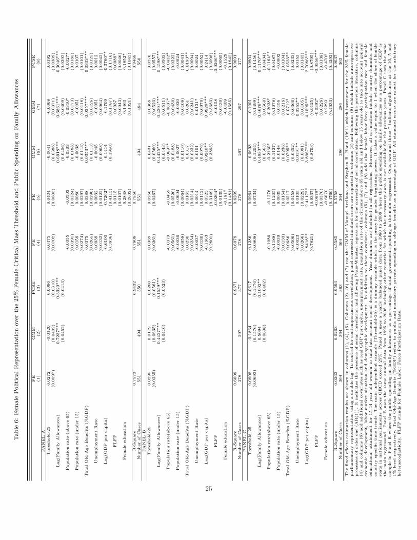
Table
6:
Fem
ale
Politi
cal
Rep
rese
nta
tion
over
the
25%
Fem
ale
Cri
tica
lM
ass
Thre
shold
and
Public
Sp
endin
gon
Fam
ily
Allow
ance
s
FE
GM
MP
CSE
FE
FE
GM
MG
MM
PC
SE
(1)
(2)
(3)
(4)
(5)
(6)
(7)
(8)
PA
NE
LA
Thre
shold
-25
0.0
272
-0.0
120
0.0
096
0.0
475
0.0
404
-0.0
041
-0.0
068
0.0
192
(0.0
597)
(0.0
402)
(0.0
310)
(0.0
702)
(0.0
605)
(0.0
386)
(0.0
371)
(0.0
309)
Lag(F
am
ily
All
ow
ances)
0.7
237***
0.3
320***
0.6
918***
0.6
861***
0.3
046***
(0.0
452)
(0.0
413)
(0.0
456)
(0.0
409)
(0.0
392)
Popula
tion
rate
(ab
ove
65)
-0.0
355
-0.0
503
-0.0
303
-0.0
310*
-0.0
327*
(0.0
391)
(0.0
324)
(0.0
188)
(0.0
173)
(0.0
185)
Popula
tion
rate
(under
15)
0.0
159
0.0
080
-0.0
038
-0.0
051
0.0
107
(0.0
274)
(0.0
297)
(0.0
113)
(0.0
118)
(0.0
101)
Tota
lO
ld-A
ge
Benefi
ts(%
GD
P)
0.0
375
0.0
388
0.0
353***
0.0
357***
0.0
333***
(0.0
265)
(0.0
290)
(0.0
113)
(0.0
126)
(0.0
125)
Unem
plo
ym
ent
Rate
0.0
039
0.0
032
-0.0
045
-0.0
051
0.0
012
(0.0
132)
(0.0
122)
(0.0
068)
(0.0
064)
(0.0
042)
Log(G
DP
per
capit
a)
-0.6
100
-0.7
262*
-0.1
414
-0.1
709
-0.3
766**
(0.3
836)
(0.4
113)
(0.1
950)
(0.1
787)
(0.1
716)
FL
FP
0.0
115
0.0
037
0.0
089*
(0.0
107)
(0.0
043)
(0.0
046)
Fem
ale
educati
on
0.2
848
0.1
463
0.1
852*
(0.2
632)
(0.1
321)
(0.1
043)
R-S
quare
0.7
573
0.9
432
0.7
808
0.7
856
0.9
468
Num
ber
of
Case
s551
494
550
551
551
494
494
550
PA
NE
LB
Thre
shold
-25
0.0
295
0.0
179
0.0
260
0.0
389
0.0
256
0.0
431
0.0
368
0.0
270
(0.0
235)
(0.0
635)
(0.0
561)
(0.0
261)
(0.0
267)
(0.0
560)
(0.0
523)
(0.0
557)
Lag(F
am
ily
All
ow
ances)
0.4
427***
0.1
559***
0.4
425***
0.4
201***
0.1
598***
(0.0
416)
(0.0
523)
(0.0
443)
(0.0
511)
(0.0
503)
Popula
tion
rate
(ab
ove
65)
-0.0
379
-0.0
459
-0.0
897*
-0.0
837*
-0.0
432*
(0.0
561)
(0.0
520)
(0.0
488)
(0.0
430)
(0.0
222)
Popula
tion
rate
(under
15)
-0.0
036
-0.0
004
-0.0
027
-0.0
020
-0.0
024
(0.0
058)
(0.0
064)
(0.0
110)
(0.0
108)
(0.0
041)
Tota
lO
ld-A
ge
Benefi
ts(%
GD
P)
0.0
230
0.0
163
0.0
317
0.0
261
0.0
193**
(0.0
234)
(0.0
214)
(0.0
232)
(0.0
241)
(0.0
094)
Unem
plo
ym
ent
Rate
-0.0
037
0.0
014
0.0
101
0.0
131*
0.0
024
(0.0
130)
(0.0
112)
(0.0
076)
(0.0
070)
(0.0
052)
Log(G
DP
per
capit
a)
-0.1
863
0.0
523
0.9
240**
0.9
929***
0.2
414
(0.2
801)
(0.3
149)
(0.3
895)
(0.3
683)
(0.3
098)
FL
FP
-0.0
264*
-0.0
158
-0.0
206***
(0.0
139)
(0.0
130)
(0.0
065)
Fem
ale
educati
on
-0.1
817
-0.0
409
-0.1
529
(0.1
481)
(0.1
585)
(0.1
842)
R-S
quare
0.6
009
0.9
671
0.6
079
0.6
209
0.9
691
Num
ber
of
Case
s378
297
377
378
378
297
297
377
PA
NE
LC
Thre
shold
-25
0.0
908
-0.1
834
0.0
617
0.1
286
0.0
964
-0.0
693
-0.1
001
0.0
804
(0.0
693)
(0.1
576)
(0.1
476)
(0.0
808)
(0.0
734)
(0.1
204)
(0.1
499)
(0.1
456)
Lag(F
am
ily
All
ow
ances)
0.5
094
0.1
002**
0.4
830***
0.4
676***
0.1
176***
(0.0
608)
(0.0
462)
(0.0
563)
(0.0
560)
(0.0
434)
Popula
tion
rate
(ab
ove
65)
-0.1
086
-0.1
276
-0.2
130*
-0.2
028*
-0.1
164**
(0.1
188)
(0.1
205)
(0.1
127)
(0.1
078)
(0.0
487)
Popula
tion
rate
(under
15)
-0.0
039
0.0
039
0.0
148
0.0
156
-0.0
002
(0.0
133)
(0.0
154)
(0.0
236)
(0.0
218)
(0.0
104)
Tota
lO
ld-A
ge
Benefi
ts(%
GD
P)
0.0
686
0.0
517
0.0
795**
0.0
712*
0.0
523**
(0.0
506)
(0.0
458)
(0.0
352)
(0.0
366)
(0.0
233)
Unem
plo
ym
ent
Rate
-0.0
023
0.0
105
0.0
191**
0.0
252**
0.0
153
(0.0
266)
(0.0
229)
(0.0
091)
(0.0
105)
(0.0
143)
Log(G
DP
per
capit
a)
1.8
418**
2.4
117**
3.8
967***
4.1
595***
2.7
086***
(0.7
821)
(0.9
337)
(0.8
703)
(0.9
125)
(0.8
795)
FL
FP
-0.0
678*
-0.0
392*
-0.0
556***
(0.0
370)
(0.0
228)
(0.0
138)
Fem
ale
educati
on
-0.6
070
0.2
293
-0.4
702
(0.4
769)
(0.4
033)
(0.4
292)
R-S
quare
0.0
263
0.0
263
0.9
593
0.5
585
0.5
758
0.9
637
Num
ber
of
Case
s364
364
363
364
364
286
286
363
The
fixed
eff
ects
est
imati
on
resu
lts
are
show
nin
colu
mns
(1),
(4),
(5).
Colu
mns
(2),
(6)
and
(7)
use
the
GM
Mof
Manuel
Are
llano
and
Ste
phen
R.
Bond
(1991)
whic
hin
stru
ment
for
the
25%
fem
ale
parl
iam
enta
ryre
pre
senta
tion
usi
ng
adouble
lag.
To
contr
ol
for
conte
mp
ora
neous
corr
ela
tion,
panel-
corr
ecte
dst
andard
err
ors
are
rep
ort
ed
incolu
mns
(3)
and
colu
mns
(8)
whic
hin
clu
de
auto
regre
ssiv
epro
cess
es
of
ord
er
one
(AR
(1))
.It
indic
ate
sth
epre
sence
of
seri
al
corr
ela
tion
and
allow
ing
Pra
is-W
inst
en
regre
ssio
nfo
rth
ecorr
ecti
on
of
seri
al
corr
ela
tion.
Follow
ing
the
pre
vio
us
lite
ratu
re,
colu
mns
(4)
and
colu
mns
(6)
add
addit
ional
covari
ate
ssu
ch
as
real
GD
Pp
er
capit
a,
unem
plo
ym
ent
rate
,p
opula
tion
rate
of
the
cit
izens
ab
ove
65
years
old
and
belo
w15
years
old
tota
ke
into
account
genera
leconom
icdevelo
pm
ent,
lab
or
mark
et
situ
ati
on
and
dem
ogra
phic
develo
pm
ent.
Inaddit
ion
toth
ese
covari
ate
s,colu
mns
(5),
(7)
and
(8)
add
als
ofe
male
lab
or
forc
epart
icip
ati
on
rate
and
fem
ale
educati
onal
att
ain
ment
for
15-4
4year
old
wom
en
tota
ke
into
account
socia
ldevelo
pm
ent.
Year
dum
mie
sare
inclu
ded
inall
regre
ssio
ns.
More
over,
all
est
imati
ons
inclu
de
countr
ydum
mie
sand
countr
ysp
ecifi
cti
me
trends.
The
main
indep
endent
vari
able
(Thre
shold
-25)
isa
dum
my
vari
able
whic
his
the
pro
xy
for
gender
barg
ain
ing
pow
er.
Itta
kes
avalu
eequal
to1
when
the
share
of
fem
ale
seats
innati
onal
parl
iam
ents
acro
ssO
EC
Dexceed
25%
.P
anel
Ause
sa
yearl
ybala
nced
panel
data
from
1980
to2008
where
the
public
spendin
gon
fam
ily
allow
ances
as
ap
erc
enta
ge
of
GD
Pis
the
main
regre
ssand.
Panel
Buse
sth
esa
me
annual
data
from
1995
to2008
inclu
din
goth
er
countr
ies
for
whic
hth
enecess
sary
data
isnot
available
for
the
pre
vio
us
years
.P
anel
Cuse
sth
esa
me
sam
ple
inP
anel
Bw
here
the
public
spendin
gon
fam
ily
allow
ances
as
ap
erc
enta
ge
of
tota
lgovenm
ent
spendin
gis
the
main
regre
ssand.
One,
two
and
thre
e*
indic
ate
signifi
cance
at
the
10,
5and
1%
level
resp
ecti
vely
.T
ota
lO
ld-A
ge
Benefi
ts(%
GD
P)
refe
rsto
public
and
mandato
rypri
vate
spendin
gon
old
-age
benefi
tsas
ap
erc
enta
ge
of
GD
P.
All
standard
err
ors
are
robust
for
the
arb
itra
ryhete
rosc
edast
icit
y.
FL
FP
stands
for
Fem
ale
Lab
or
Forc
eP
art
icip
ati
on
Rate
.
25
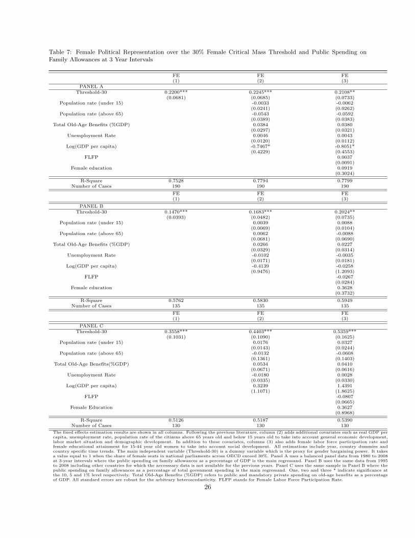
Table 7: Female Political Representation over the 30% Female Critical Mass Threshold and Public Spending onFamily Allowances at 3 Year Intervals
FE FE FE(1) (2) (3)
PANEL AThreshold-30 0.2200*** 0.2245*** 0.2108**
(0.0681) (0.0685) (0.0733)Population rate (under 15) -0.0033 -0.0062
(0.0241) (0.0262)Population rate (above 65) -0.0543 -0.0592
(0.0389) (0.0383)Total Old-Age Benefits (%GDP) 0.0384 0.0380
(0.0297) (0.0321)Unemployment Rate 0.0046 0.0043
(0.0120) (0.0112)Log(GDP per capita) -0.7467* -0.8051*
(0.4229) (0.4553)FLFP 0.0037
(0.0091)Female education 0.0919
(0.3024)
R-Square 0.7528 0.7794 0.7799Number of Cases 190 190 190
FE FE FE(1) (2) (3)
PANEL BThreshold-30 0.1470*** 0.1683*** 0.2024**
(0.0393) (0.0482) (0.0735)Population rate (under 15) 0.0039 0.0088
(0.0069) (0.0104)Population rate (above 65) 0.0062 -0.0088
(0.0681) (0.0690)Total Old-Age Benefits (%GDP) 0.0266 0.0227
(0.0329) (0.0314)Unemployment Rate -0.0102 -0.0035
(0.0171) (0.0181)Log(GDP per capita) -0.4139 -0.0258
(0.9476) (1.2093)FLFP -0.0267
(0.0284)Female education 0.3628
(0.3732)
R-Square 0.5762 0.5830 0.5949Number of Cases 135 135 135
FE FE FE(1) (2) (3)
PANEL CThreshold-30 0.3558*** 0.4403*** 0.5359***
(0.1031) (0.1090) (0.1625)Population rate (under 15) 0.0176 0.0327
(0.0143) (0.0244)Population rate (above 65) -0.0132 -0.0608
(0.1361) (0.1403)Total Old-Age Benefits(%GDP) 0.0534 0.0410
(0.0671) (0.0616)Unemployment Rate -0.0180 0.0028
(0.0335) (0.0330)Log(GDP per capita) 0.3239 1.4391
(1.1071) (1.8625)FLFP -0.0807
(0.0665)Female Education 0.3627
(0.8968)
R-Square 0.5126 0.5187 0.5390Number of Cases 130 130 130
The fixed effects estimation results are shown in all columns. Following the previous literature, column (2) adds additional covariates such as real GDP percapita, unemployment rate, population rate of the citizens above 65 years old and below 15 years old to take into account general economic development,labor market situation and demographic development. In addition to these covariates, columns (3) also adds female labor force participation rate andfemale educational attainment for 15-44 year old women to take into account social development. All estimations include year, country dummies andcountry specific time trends. The main independent variable (Threshold-30) is a dummy variable which is the proxy for gender bargaining power. It takesa value equal to 1 when the share of female seats in national parliaments across OECD exceed 30%. Panel A uses a balanced panel data from 1980 to 2008at 3-year intervals where the public spending on family allowances as a percentage of GDP is the main regressand. Panel B uses the same data from 1995to 2008 including other countries for which the necesssary data is not available for the previous years. Panel C uses the same sample in Panel B where thepublic spending on family allowances as a percentage of total govenment spending is the main regressand. One, two and three * indicate significance atthe 10, 5 and 1% level respectively. Total Old-Age Benefits (%GDP) refers to public and mandatory private spending on old-age benefits as a percentageof GDP. All standard errors are robust for the arbitrary heteroscedasticity. FLFP stands for Female Labor Force Participation Rate.
26
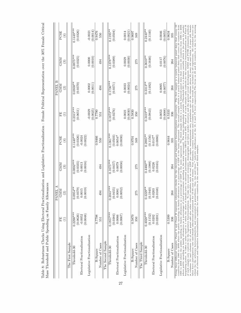
Table
8:
Robust
nes
sC
hec
ks
Usi
ng
Ele
ctora
lF
ract
ionaliza
tion
and
Leg
isla
tive
Fra
ctio
naliza
tion
:F
emale
Politi
cal
Rep
rese
nta
tion
over
the
30%
Fem
ale
Cri
tica
lM
ass
Thre
shold
and
Public
Sp
endin
gon
Fam
ily
Allow
ance
s
PA
NE
LA
PA
NE
LB
FE
GM
MG
MM
PC
SE
FE
GM
MG
MM
PC
SE
(1)
(2)
(3)
(4)
(1)
(2)
(3)
(4)
Th
eF
irst
Sam
ple
Th
resh
old
-30
0.2
290***
0.0
954**
0.0
892***
0.1
440***
0.2
315***
0.0
938**
0.0
875***
0.1
449***
(0.0
626)
(0.0
379)
(0.0
335)
(0.0
326)
(0.0
651)
(0.0
370)
(0.0
325)
(0.0
326)
Ele
ctora
lF
ract
ion
aliza
tion
-0.0
052
0.0
015
0.0
013
-0.0
024
(0.0
048)
(0.0
019)
(0.0
016)
(0.0
022)
Leg
isla
tive
Fra
ctio
naliza
tion
-0.0
029
0.0
002
0.0
000
-0.0
021
(0.0
025)
(0.0
011)
(0.0
010)
(0.0
014)
R-S
qu
are
0.7
798
0.9
466
0.7
790
0.9
476
Nu
mb
erof
Case
s551
494
494
550
551
494
494
550
Th
eS
econ
dS
am
ple
Th
resh
old
-30
0.1
857***
0.2
041***
0.1
675***
0.1
361***
0.1
672***
0.1
736***
0.1
378***
0.1
195**
(0.0
384)
(0.0
455)
(0.0
457)
(0.0
503)
(0.0
276)
(0.0
371)
(0.0
389)
(0.0
504)
Ele
ctora
lF
ract
ion
aliza
tion
0.0
066
0.0
081
0.0
079
0.0
054*
(0.0
067)
(0.0
052)
(0.0
056)
(0.0
030)
Leg
isla
tive
Fra
ctio
naliza
tion
0.0
021
0.0
033
0.0
029
0.0
014
(0.0
030)
(0.0
024)
(0.0
030)
(0.0
021)
R-S
qu
are
0.5
870
0.9
701
0.5
830
0.9
697
Nu
mb
erof
Case
s350
275
275
349
350
275
275
349
Th
eT
hir
dS
am
ple
Th
resh
old
-30
0.4
028***
0.4
229**
0.4
460**
0.2
885**
0.3
419***
0.3
313**
0.3
610**
0.2
440**
(0.1
152)
(0.1
940)
(0.1
988)
(0.1
156)
(0.0
843)
(0.1
492)
(0.1
646)
(0.1
140)
Ele
ctora
lF
ract
ion
aliza
tion
0.0
202
0.0
203
0.0
226
0.0
147*
(0.0
201)
(0.0
168)
(0.0
165)
(0.0
080)
Leg
isla
tive
Fra
ctio
naliza
tion
0.0
053
0.0
095
0.0
117
0.0
046
(0.0
088)
(0.0
077)
(0.0
076)
(0.0
055)
R-S
qu
are
0.5
399
0.9
644
0.5
333
0.9
634
Nu
mb
erof
Case
s336
264
264
335
336
264
264
335
Usin
gthree
diffe
rent
sam
ple
s,
PanelA
and
PanelB
represent
robustness
checks
for
the
ele
ctoraland
legisla
tiv
efractio
nalizatio
nrespectiv
ely
.The
first
sam
ple
isa
yearly
bala
nced
paneldata
that
covers
19
countrie
sfrom
1980
to
2008
where
the
public
spendin
gon
fam
ily
allowances
as
apercentage
ofG
DP
isthe
main
regressand.
The
second
sam
ple
which
isa
yearly
bala
nced
paneldata
that
covers
25
countrie
sfrom
1995
to
2008
where
the
public
spendin
gon
fam
ily
allowances
as
apercentage
ofG
DP
isthe
main
regressand.
The
third
sam
ple
which
isa
yearly
bala
nced
paneldata
that
covers
24
countrie
sfrom
1995
to
2008
where
public
spendin
gon
fam
ily
allowances
as
apercentage
oftotalgovernm
ent
spendin
gis
the
main
regressand.
The
main
independent
varia
ble
(Threshold
-30)
isa
dum
my
varia
ble
which
isthe
proxy
for
gender
bargain
ing
power.
Ittakes
avalu
eequalto
1when
the
share
offe
male
seats
innatio
nalparliam
ents
across
OECD
exceed
30%
.PanelA
ofeach
sam
ple
only
controls
for
the
ele
ctoralfractio
nalizatio
nand
PanelB
ofeach
sam
ple
only
controls
for
the
legisla
tiv
efractio
nalizatio
n.
To
take
into
account
econom
ic,dem
ographic
and
labor
market
situatio
nand
the
generalsocia
ldevelo
pm
ent,G
MM
and
PCSE
estim
atio
nm
ethods
incolu
mns
(3)
and
colu
mns
(4)
ofeach
paneladd
also
other
controlvaria
ble
ssuch
as
realG
DP
per
capita,unem
plo
ym
ent
rate,popula
tio
nrate
ofthe
citiz
ens
above
65
years
old
and
belo
w15
years
old
,fe
male
laborfo
rce
partic
ipatio
nrate
and
fem
ale
educatio
nalattain
mentfo
r15-4
4yearold
wom
en.
Yeardum
mie
s,country
dum
mie
sand
country
specific
tim
etrendsare
inclu
ded
inall
regressio
ns.
All
standard
errorsare
robust
for
the
arbitrary
heteroscedastic
ity
and
represented
inparentheses.
One,two
and
three
*in
dic
ate
sig
nific
ance
at
the
10,5
and
1%
levelrespectiv
ely
.The
focus
on
25
and
24
countrie
sis
due
to
the
missin
gvalu
eofele
ctoraland
legisla
tiv
efractio
nalizatio
nvaria
ble
sfo
rsom
ecountrie
sin
the
second
and
third
sam
ple
s.
27
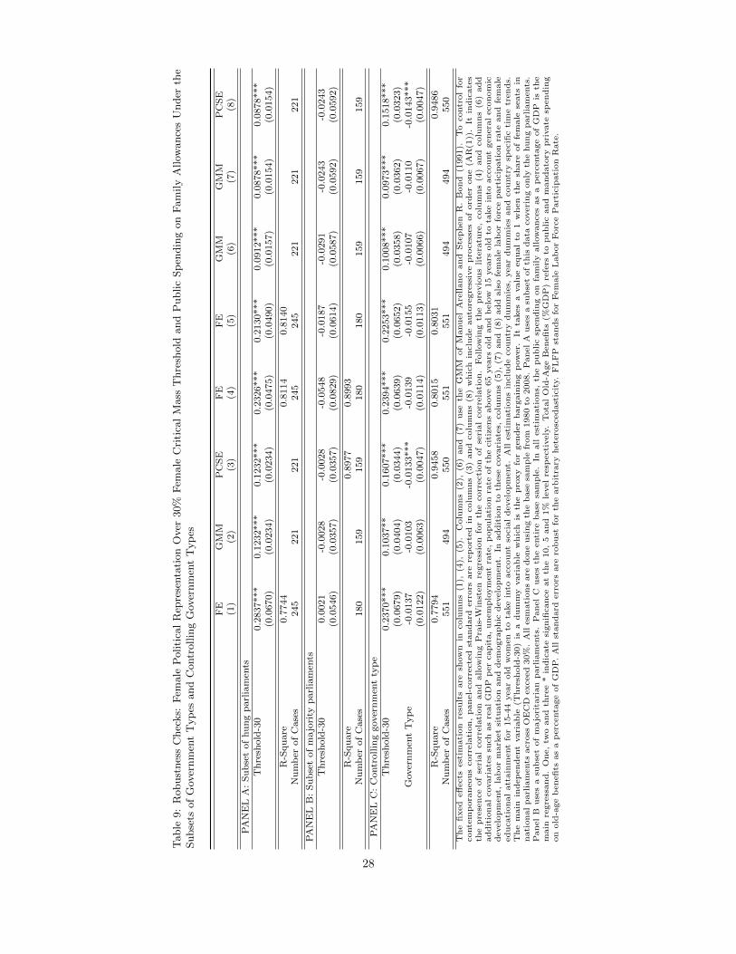
Table
9:
Robust
nes
sC
hec
ks:
Fem
ale
Politi
cal
Rep
rese
nta
tion
Over
30%
Fem
ale
Cri
tica
lM
ass
Thre
shold
and
Public
Sp
endin
gon
Fam
ily
Allow
ance
sU
nder
the
Subse
tsof
Gov
ernm
ent
Typ
esand
Contr
ollin
gG
over
nm
ent
Typ
es
FE
GM
MP
CS
EF
EF
EG
MM
GM
MP
CS
E(1
)(2
)(3
)(4
)(5
)(6
)(7
)(8
)
PA
NE
LA
:S
ub
set
of
hu
ng
parl
iam
ents
Th
resh
old
-30
0.2
837***
0.1
232***
0.1
232***
0.2
326***
0.2
130***
0.0
912***
0.0
878***
0.0
878***
(0.0
670)
(0.0
234)
(0.0
234)
(0.0
475)
(0.0
490)
(0.0
157)
(0.0
154)
(0.0
154)
R-S
qu
are
0.7
744
0.8
114
0.8
140
Nu
mb
erof
Case
s245
221
221
245
245
221
221
221
PA
NE
LB
:S
ub
set
of
ma
jori
typ
arl
iam
ents
Th
resh
old
-30
0.0
021
-0.0
028
-0.0
028
-0.0
548
-0.0
187
-0.0
291
-0.0
243
-0.0
243
(0.0
546)
(0.0
357)
(0.0
357)
(0.0
829)
(0.0
614)
(0.0
587)
(0.0
592)
(0.0
592)
R-S
qu
are
0.8
977
0.8
993
Nu
mb
erof
Case
s180
159
159
180
180
159
159
159
PA
NE
LC
:C
ontr
ollin
ggover
nm
ent
typ
eT
hre
shold
-30
0.2
370***
0.1
037**
0.1
607***
0.2
394***
0.2
253***
0.1
008***
0.0
973***
0.1
518***
(0.0
679)
(0.0
404)
(0.0
344)
(0.0
639)
(0.0
652)
(0.0
358)
(0.0
362)
(0.0
323)
Gover
nm
ent
Typ
e-0
.0137
-0.0
103
-0.0
133***
-0.0
139
-0.0
155
-0.0
107
-0.0
110
-0.0
143***
(0.0
122)
(0.0
063)
(0.0
047)
(0.0
114)
(0.0
113)
(0.0
066)
(0.0
067)
(0.0
047)
R-S
qu
are
0.7
794
0.9
458
0.8
015
0.8
031
0.9
486
Nu
mb
erof
Case
s551
494
550
551
551
494
494
550
The
fixed
eff
ects
est
imati
on
resu
lts
are
show
nin
colu
mns
(1),
(4),
(5).
Colu
mns
(2),
(6)
and
(7)
use
the
GM
Mof
Manuel
Are
llano
and
Ste
phen
R.
Bond
(1991).
To
contr
ol
for
conte
mp
ora
neous
corr
ela
tion,
panel-
corr
ecte
dst
andard
err
ors
are
rep
ort
ed
incolu
mns
(3)
and
colu
mns
(8)
whic
hin
clu
de
auto
regre
ssiv
epro
cess
es
of
ord
er
one
(AR
(1))
.It
indic
ate
sth
epre
sence
of
seri
al
corr
ela
tion
and
allow
ing
Pra
is-W
inst
en
regre
ssio
nfo
rth
ecorr
ecti
on
of
seri
al
corr
ela
tion.
Follow
ing
the
pre
vio
us
lite
ratu
re,
colu
mns
(4)
and
colu
mns
(6)
add
addit
ional
covari
ate
ssu
chas
real
GD
Pp
er
capit
a,
unem
plo
ym
ent
rate
,p
opula
tion
rate
of
the
cit
izens
ab
ove
65
years
old
and
belo
w15
years
old
tota
ke
into
account
genera
leconom
icdevelo
pm
ent,
lab
or
mark
et
situ
ati
on
and
dem
ogra
phic
develo
pm
ent.
Inaddit
ion
toth
ese
covari
ate
s,colu
mns
(5),
(7)
and
(8)
add
als
ofe
male
lab
or
forc
epart
icip
ati
on
rate
and
fem
ale
educati
onal
att
ain
ment
for
15-4
4year
old
wom
en
tota
ke
into
account
socia
ldevelo
pm
ent.
All
est
imati
ons
inclu
de
countr
ydum
mie
s,year
dum
mie
sand
countr
ysp
ecifi
cti
me
trends.
The
main
indep
endent
vari
able
(Thre
shold
-30)
isa
dum
my
vari
able
whic
his
the
pro
xy
for
gender
barg
ain
ing
pow
er.
Itta
kes
avalu
eequal
to1
when
the
share
of
fem
ale
seats
innati
onal
parl
iam
ents
acro
ssO
EC
Dexceed
30%
.A
llesm
ati
ons
are
done
usi
ng
the
base
sam
ple
from
1980
to2008.
Panel
Ause
sa
subse
tof
this
data
coveri
ng
only
the
hung
parl
iam
ents
.P
anel
Buse
sa
subse
tof
majo
rita
rian
parl
iam
ents
.P
anel
Cuse
sth
eenti
rebase
sam
ple
.In
all
est
imati
ons,
the
public
spendin
gon
fam
ily
allow
ances
as
ap
erc
enta
ge
of
GD
Pis
the
main
regre
ssand.
One,
two
and
thre
e*
indic
ate
signifi
cance
at
the
10,
5and
1%
level
resp
ecti
vely
.T
ota
lO
ld-A
ge
Benefits
(%G
DP
)re
fers
topublic
and
mandato
rypri
vate
spendin
gon
old
-age
benefits
as
ap
erc
enta
ge
of
GD
P.
All
standard
err
ors
are
robust
for
the
arb
itra
ryhete
rosc
edast
icit
y.
FL
FP
stands
for
Fem
ale
Lab
or
Forc
eP
art
icip
ati
on
Rate
.
28
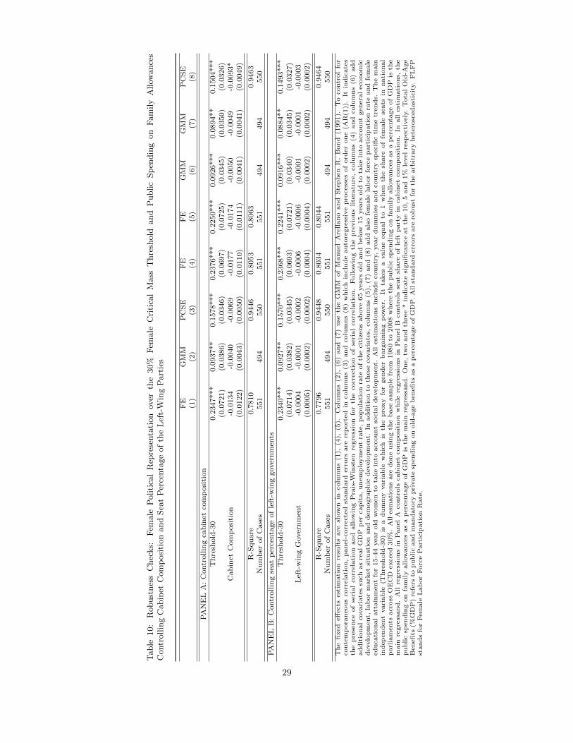
Table
10:
Robust
nes
sC
hec
ks:
Fem
ale
Politi
cal
Rep
rese
nta
tion
over
the
30%
Fem
ale
Cri
tica
lM
ass
Thre
shold
and
Public
Sp
endin
gon
Fam
ily
Allow
ance
sC
ontr
ollin
gC
abin
etC
om
posi
tion
and
Sea
tP
erce
nta
ge
of
the
Lef
t-W
ing
Part
ies
FE
GM
MP
CS
EF
EF
EG
MM
GM
MP
CS
E(1
)(2
)(3
)(4
)(5
)(6
)(7
)(8
)
PA
NE
LA
:C
ontr
ollin
gca
bin
etco
mp
osi
tion
Th
resh
old
-30
0.2
347***
0.0
937**
0.1
578***
0.2
376***
0.2
250***
0.0
926***
0.0
894**
0.1
504***
(0.0
721)
(0.0
386)
(0.0
346)
(0.0
697)
(0.0
725)
(0.0
345)
(0.0
350)
(0.0
326)
Cab
inet
Com
posi
tion
-0.0
134
-0.0
040
-0.0
069
-0.0
177
-0.0
174
-0.0
050
-0.0
049
-0.0
093*
(0.0
122)
(0.0
043)
(0.0
050)
(0.0
110)
(0.0
111)
(0.0
041)
(0.0
041)
(0.0
049)
R-S
qu
are
0.7
810
0.9
446
0.8
053
0.8
063
0.9
463
Nu
mb
erof
Case
s551
494
550
551
551
494
494
550
PA
NE
LB
:C
ontr
ollin
gse
at
per
centa
ge
of
left
-win
ggover
nm
ents
Th
resh
old
-30
0.2
340***
0.0
927**
0.1
570***
0.2
368***
0.2
241***
0.0
916***
0.0
884**
0.1
493***
(0.0
714)
(0.0
382)
(0.0
345)
(0.0
693)
(0.0
721)
(0.0
340)
(0.0
345)
(0.0
327)
Lef
t-w
ing
Gover
nm
ent
-0.0
004
-0.0
001
-0.0
002
-0.0
006
-0.0
006
-0.0
001
-0.0
001
-0.0
003
(0.0
005)
(0.0
002)
(0.0
002)
(0.0
004)
(0.0
004)
(0.0
002)
(0.0
002)
(0.0
002)
R-S
qu
are
0.7
796
0.9
448
0.8
034
0.8
044
0.9
464
Nu
mb
erof
Case
s551
494
550
551
551
494
494
550
The
fixed
eff
ects
est
imati
on
resu
lts
are
show
nin
colu
mns
(1),
(4),
(5).
Colu
mns
(2),
(6)
and
(7)
use
the
GM
Mof
Manuel
Are
llano
and
Ste
phen
R.
Bond
(1991).
To
contr
ol
for
conte
mp
ora
neous
corr
ela
tion,
panel-
corr
ecte
dst
andard
err
ors
are
rep
ort
ed
incolu
mns
(3)
and
colu
mns
(8)
whic
hin
clu
de
auto
regre
ssiv
epro
cess
es
of
ord
er
one
(AR
(1))
.It
indic
ate
sth
epre
sence
of
seri
al
corr
ela
tion
and
allow
ing
Pra
is-W
inst
en
regre
ssio
nfo
rth
ecorr
ecti
on
of
seri
al
corr
ela
tion.
Follow
ing
the
pre
vio
us
lite
ratu
re,
colu
mns
(4)
and
colu
mns
(6)
add
addit
ional
covari
ate
ssu
chas
real
GD
Pp
er
capit
a,
unem
plo
ym
ent
rate
,p
opula
tion
rate
of
the
cit
izens
ab
ove
65
years
old
and
belo
w15
years
old
tota
ke
into
account
genera
leconom
icdevelo
pm
ent,
lab
or
mark
et
situ
ati
on
and
dem
ogra
phic
develo
pm
ent.
Inaddit
ion
toth
ese
covari
ate
s,colu
mns
(5),
(7)
and
(8)
add
als
ofe
male
lab
or
forc
epart
icip
ati
on
rate
and
fem
ale
educati
onal
att
ain
ment
for
15-4
4year
old
wom
en
tota
ke
into
account
socia
ldevelo
pm
ent.
All
est
imati
ons
inclu
de
countr
y,
year
dum
mie
sand
countr
ysp
ecifi
cti
me
trends.
The
main
indep
endent
vari
able
(Thre
shold
-30)
isa
dum
my
vari
able
whic
his
the
pro
xy
for
gender
barg
ain
ing
pow
er.
Itta
kes
avalu
eequal
to1
when
the
share
of
fem
ale
seats
innati
onal
parl
iam
ents
acro
ssO
EC
Dexceed
30%
.A
llesm
ati
ons
are
done
usi
ng
the
base
sam
ple
from
1980
to2008
where
the
public
spendin
gon
fam
ily
allow
ances
as
ap
erc
enta
ge
of
GD
Pis
the
main
regre
ssand.
All
regre
ssio
ns
inP
anel
Acontr
ols
cabin
et
com
posi
tion
while
regre
ssio
ns
inP
anel
Bcontr
ols
seat
share
of
left
part
yin
cabin
et
com
posi
tion.
Inall
est
imati
ons,
the
public
spendin
gon
fam
ily
allow
ances
as
ap
erc
enta
ge
of
GD
Pis
the
main
regre
ssand.
One,
two
and
thre
e*
indic
ate
signifi
cance
at
the
10,
5and
1%
level
resp
ecti
vely
.T
ota
lO
ld-A
ge
Benefits
(%G
DP
)re
fers
topublic
and
mandato
rypri
vate
spendin
gon
old
-age
benefits
as
ap
erc
enta
ge
of
GD
P.
All
standard
err
ors
are
robust
for
the
arb
itra
ryhete
rosc
edast
icit
y.
FL
FP
stands
for
Fem
ale
Lab
or
Forc
eP
art
icip
ati
on
Rate
.
29
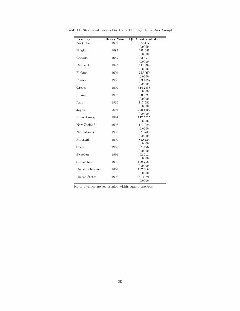
Table 11: Structural Breaks For Every Country Using Base Sample
Country Break Year QLR test statisticAustralia 1991 67.5117
[0.0000]Belgium 1985 225.941
[0.0000]Canada 1985 583.5519
[0.0000]Denmark 1987 49.4299
[0.0000]Finland 1991 75.5060
[0.0000]France 1986 353.4097
[0.0000]Greece 1990 314.7958
[0.0000]Ireland 1992 63.929
[0.0000]Italy 1986 115.593
[0.0000]Japan 2001 220.1292
[0.0000]Luxembourg 1992 117.5735
[0.0000]New Zealand 1996 171.925
[0.0000]Netherlands 1987 62.3748
[0.0000]Portugal 1990 83.8733
[0.0000]Spain 1986 92.0637
[0.0000]Sweeden 1991 52.212
[0.0000]Switzerland 1996 122.7585
[0.0000]United Kingdom 1991 197.0192
[0.0000]United States 1992 81.1321
[0.0000]
Note: p-values are represented within square brackets.
30
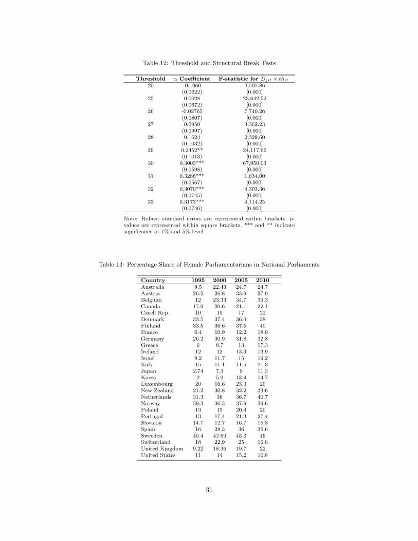
Table 12: Threshold and Structural Break Tests
Threshold α Coefficient F-statistic for Djit × thit20 -0.1060 4,507.86
(0.0622) [0.000]25 0.0028 23,642.52
(0.0672) [0.000]26 -0.02765 7,740.26
(0.0807) [0.000]27 0.0950 3,362.23
(0.0997) [0.000]28 0.1624 2,329.60
(0.1032) [0.000]29 0.2452** 24,117.66
(0.1013) [0.000]30 0.3003*** 67,950.03
(0.0598) [0.000]31 0.3288*** 1,634.00
(0.0567) [0.000]32 0.3070*** 4,303.36
(0.0745) [0.000]33 0.3173*** 4,114.25
(0.0746) [0.000]
Note: Robust standard errors are represented within brackets, p-values are represented within square brackets, *** and ** indicatesignificance at 1% and 5% level.
Table 13: Percentage Share of Female Parliamentarians in National Parliaments
Country 1995 2000 2005 2010Australia 9.5 22.43 24.7 24.7Austria 26.2 26.8 33.9 27.9Belgium 12 23.33 34.7 39.3Canada 17.9 20.6 21.1 22.1Czech Rep. 10 15 17 22Denmark 33.5 37.4 36.9 38Finland 33.5 36.6 37.5 40France 6.4 10.9 12.2 18.9Germany 26.2 30.9 31.8 32.8Greece 6 8.7 13 17.3Ireland 12 12 13.3 13.9Israel 9.2 11.7 15 19.2Italy 15 11.1 11.5 21.3Japan 2.74 7.3 9 11.3Korea 2 5.9 13.4 14.7Luxembourg 20 16.6 23.3 20New Zealand 21.2 30.8 32.2 33.6Netherlands 31.3 36 36.7 40.7Norway 39.3 36.3 37.9 39.6Poland 13 13 20.4 20Portugal 13 17.4 21.3 27.4Slovakia 14.7 12.7 16.7 15.3Spain 16 28.3 36 36.6Sweeden 40.4 42.69 45.3 45Switzerland 18 22.9 25 16.8United Kingdom 9.22 18.36 19.7 22United States 11 14 15.2 16.8
31
References
Alesina, A. and La Ferrara, E. (2005). Preferences for redistribution in the land of opportunities. Journal
of Public Economics, 89(5):897–931.
Andrews, D. W. (1993). Tests for parameter instability and structural change with unknown change point.
Econometrica: Journal of the Econometric Society, pages 821–856.
Arellano, M. and Bond, S. (1991). Some tests of specification for panel data: Monte carlo evidence and an
application to employment equations. The Review of Economic Studies, 58(2):277–297.
Armingeon, K., Weisstanner, D., Engler, S., Potolidis, P., and Gerber, M. (2012). Comparative political
data set i, 1960-2010. Technical report, Bern:Institute of Political Science, University of Bern.
Ashworth, J., Geys, B., and Heyndels, B. (2012). Gender quotas, female representation and public expendi-
tures: New evidence from flemish municipalities. In 2nd World Congress of the Public Choice Societies,
Miami, pages 8–11.
Astrid, B. and Tenorio, Z. (2014). Social spending responses to organized labor and mass protests in latin
america, 1970-2007. Comparative Political Studies, 47(14):1945–1972.
Bawn, K. and Rosenbluth, F. (2006). Short versus long coalitions: electoral accountability and the size of
the public sector. American Journal of Political Science, 50(2):251–265.
Beck, N. and Katz, J. N. (1995). What to do (and not to do) with time-series cross-section data. American
political science review, pages 634–647.
Beck, N. and Katz, J. N. (1996). Nuisance vs. substance: Specifying and estimating time-series-cross-section
models. Political analysis, 6(1):1–36.
Beckwith, K. and Cowell-Meyers, K. (2007). Sheer numbers: Critical representation thresholds and women’s
political representation. Perspectives on Politics, pages 553–565.
Besley, T. and Case, A. (2000). Unnatural experiments? estimating the incidence of endogenous policies.
The Economic Journal, 110(467):672–694.
Besley, T. and Coate, S. (1997). An economic model of representative democracy. The Quarterly Journal of
Economics, 112(1):85–114.
32
Bolzendahl, C. and Brooks, C. (2007). Women’s political representation and welfare state spending in 12
capitalist democracies. Social Forces, 85(4):1509–1534.
Bonoli, G. and Reber, F. (2010). The political economy of childcare in oecd countries: Explaining cross-
national variation in spending and coverage rates. European Journal of Political Research, 49(1):97–118.
Case, A. and Deaton, A. (1998). Large cash transfers to the elderly in south africa. The Economic Journal,
108(450):1330–1361.
Chattopadhyay, R. and Duflo, E. (2004). Women as policy makers: Evidence from a randomized policy
experiment in india. Econometrica, 72(5):1409–1443.
Chen, L.-J. (2010). Do gender quotas influence women’s representation and policies? The European Journal
of Comparative Economics, 7(1):13–60.
Dahlerup, D. (1988). From a small to a large minority: women in scandinavian politics. Scandinavian
Political Studies, 11(4):275–298.
Diamond, P. and Lodge, G. (2013). European welfare states after the crisis. Policy Network.
Dodson, D. L. and Carroll, S. J. (1991). Reshaping the agenda: Women in state legislatures. Eagleton
Institute of Politics, Rutgers, the State University of New Jersey.
Downs, A. (1957). An economic theory of political action in a democracy. The Journal of Political Economy,
65(2):135–150.
Duflo, E. (2003). Grandmothers and granddaughters: Old-age pensions and intrahousehold allocation in
south africa. The World Bank Economic Review, 17(1):1–25.
Duflo, E. (2012). Women empowerment and economic development. Journal of Economic Literature,
50(4):1051–1079.
Edlund, L. and Pande, R. (2002). Why have women become left-wing? the political gender gap and the
decline in marriage. The Quarterly Journal of Economics, 117(3):917–961.
Erhel, C. and Guergoat-Lariviere, M. (2013). Labor market regimes, family policies, and women’s behavior
in the eu. Feminist Economics, 19(4):76–109.
Fortin, N. M. (2005). Gender role attitudes and the labour-market outcomes of women across oecd countries.
oxford review of Economic Policy, 21(3):416–438.
33
Guinier, L. (1994). The Tyranny of the majority: Fundamental Fairness in Representative Democracy. Free
Press New York.
Heston, A., Summers, R., and Aten, B. (2012). Penn world table 7.1. Center for International Comparisons
of Production, Income and Prices at the University of Pennsylvania.
IHME (2010). Educational attainment and child mortality estimates by country 1970-2009. Technical report,
Institute for Health Metrics and Evaluation. Seattle, United States.
ILO (2012). Online key indicators of the labour market database, 6th edition. Technical report, International
Labor Organization.
IPU (1995). Women in parliaments:1945-1995. Worldwide Statistical Survey ISBN 92 / 9142 / 008-5,
Inter-Parliamentary Union.
Jones, M. P. (1997). Legislator gender and legislator policy priorities in the argentine chamber of deputies
and the united states house of representatives. Policy Studies Journal, 25(4):613–629.
Kanter, R. (1977). Men and Women of the Corporation, volume 5049. Basic books.
Kittilson, M. C. (2008). Representing women: The adoption of family leave in comparative perspective. The
Journal of Politics, 70(02):323–334.
Kontopoulos, Y. and Perotti, R. (1999). Government fragmentation and fiscal policy outcomes: Evidence
from oecd countries. In Fiscal institutions and fiscal performance, pages 81–102. University of Chicago
Press.
Lijphart, A. (2012). Patterns of Democracy: Government Forms and Performance in Thirty-Six Countries.
Yale University Press.
Liphart, A. (1977). Democracy in plural societies: A comparative exploration. Yale University Press.
Lovenduski, J. and Norris, P. (2003). Westminster women: The politics of presence. Political studies,
51(1):84–102.
Lundberg, S. and Pollak, R. A. (1993). Separate spheres bargaining and the marriage market. Journal of
Political Economy, pages 988–1010.
Manser, M. and Brown, M. (1980). Marriage and household decision-making: A bargaining analysis. Inter-
national Economic Review, 21(1):31–44.
34
Mavisakalyan, A. (2014). Women in cabinet and public health spending: evidence across countries. Eco-
nomics of Governance, pages 1–24.
McElroy, M. B. and Horney, M. J. (1981). Nash-bargained household decisions: Toward a generalization of
the theory of demand. International Economic Review, 22(2):333–349.
Mueller, D. C. and Murrell, P. (1986). Interest groups and the size of government. Public Choice, 48(2):125–
145.
Nickell, S. (1981). Biases in dynamic models with fixed effects. Econometrica: Journal of the Econometric
Society, pages 1417–1426.
OECD (2010). Labour force statistics: Summary tables. Technical report, OECD Employment and Labour
Market Statistics (database).
OECD (2011). Society at a glance. Technical report, Organisation for Economic Cooperation and Develop-
ment.
OECD (2012). Social spending during the crisis, social expenditure (socx) data update 2012. Technical
report, Organisation for Economic Cooperation and Development.
OECD (2013). Social expenditure statistics: Aggregated data. Technical report, Organisation for Economic
Cooperation and Development.
Osborne, M. J. and Slivinski, A. (1996). A model of political competition with citizen-candidates. The
Quarterly Journal of Economics, 111(1):65–96.
Pande, R. (2003). Can mandated political representation increase policy influence for disadvantaged minori-
ties? theory and evidence from india. The American Economic Review, 93(4):1132–1151.
Perotti, R. and Kontopoulos, Y. (2002). Fragmented fiscal policy. Journal of Public Economics, 86(2):191–
222.
Persson, T. and Tabellini, G. (2004). Constitutional rules and fiscal policy outcomes. American Economic
Review, pages 25–45.
Phillips, A. (1995). The Politics of Presence. Oxford University Press.
Potrafke, N. and Ursprung, H. W. (2012). Globalization and gender equality in the course of development.
European Journal of Political Economy, 28(4):399–413.
35
Quandt, R. E. (1960). Tests of the hypothesis that a linear regression system obeys two separate regimes.
Journal of the American statistical Association, 55(290):324–330.
Rae, D. (1968). A note on the fractionalization of some european party systems. Comparative Political
Studies, 1(3):413–418.
Rehavi, M. M. (2007). Sex and politics: Do female legislators affect state spending. Unpublished manuscript,
University of Michigan.
Rigon, M. and Tanzi, G. M. (2011). Does gender matter for public spending? empirical evidence from italian
municipalities. Technical Report 862, Bank of Italy, Economic Research and International Relations Area,
Temi di discussion.
Roubini, N. and Sachs, J. D. (1989). Political and economic determinants of budget deficits in the industrial
democracies. European Economic Review, 33(5):903–933.
Ruhm, C. J. (2000). Parental leave and child health. Journal of Health Economics, 19(6):931–960.
Studlar, D. T. and McAllister, I. (2002). Does a critical mass exist? a comparative analysis of women’s
legislative representation since 1950. European Journal of Political Research, 41(2):233–253.
Svaleryd, H. (2009). Women’s representation and public spending. European Journal of Political Economy,
25(2):186–198.
Tanaka, S. (2005). Parental leave and child health across oecd countries*. The Economic Journal,
115(501):F7–F28.
Thomas, D. (1990). Intra-household resource allocation: An inferential approach. Journal of Human Re-
sources, pages 635–664.
Thomas, S. (1991). The impact of women on state legislative policies. The Journal of Politics, 53(04):958–
976.
Thomas, S. (1994). How Women Legislate? Oxford University Press New York.
UN (2012). “World Population Prospects: The 2012 Revision”. Technical report, United Nations, Depart-
ment of Economic and Social Affairs, Population Division, Population Estimates and Projections Section.
UN (2013). The millennium development goals report. Technical report, United Nations, New York.
36
Volkerink, B. and De Haan, J. (2001). Fragmented government effects on fiscal policy: New evidence. Public
Choice, 109(3-4):221–242.
Wangnerud, L. (2009). Women in parliaments: Descriptive and substantive representation. Annual Review
of Political Science, 12:51–69.
Young, I. M. (2002). Inclusion and Democracy. Oxford University Press.
37