GEMINI 8-M TELESCOPES PROJECT · Study", Systems Technology ... Thompson, P. Phd, "Keck Telescope Elevation AxisServo Design Evaluation and Feasibility Study", ... for a baseline

GEMINI 8-M TELESCOPES PROJECT

CONTROLS GROUP

GEMINI NONLINEAR

SERVO SIMULATION

DOCUMENT NUMBER: TN-C-G0022 ISSUE NUMBER: 001 REVISION NUMBER: 1.1 DATE: 3 NOVEMBER 1994 PREPARED BY: M.K.BURNS (GEMINI) AND JOHN WILKES (RGO) APPROVED BY: R.J.MCGONEGAL SYSTEMS: J. OSCHMANN PROPRIETARY/NON-DISCLOSURE: NO PROCUREMENT SENSISTIVE: NO

TN-C-G0022

Page 2

Contents LIST OF FIGURES................................................................................................................... 3 LIST OF APPENDICES............................................................................................................ 5 LIST OF TABLES ..................................................................................................................... 6 1.0 SUMMARY........................................................................................................................ 7 2.0 INTRODUCTION .............................................................................................................. 8 3.0 LINE OF SIGHT IMAGE EQUATIONS............................................................................ 9 4.0 STRUCTURES: PIER, MOUNT, TUBE, CASSEGRAIN, SECONDARY....................... 10

4.1 PIER............................................................................................................................. 10 4.2 MOUNT........................................................................................................................ 11 4.3 TUBE ........................................................................................................................... 11 4.4 CASSEGRAIN ................................................................................................................ 12 4.5 SECONDARY MIRROR................................................................................................... 12

5.0 DRIVES AND BEARINGS .............................................................................................. 13 5.1 AZIMUTH DRIVE .......................................................................................................... 14 5.2 ALTITUDE DRIVE.......................................................................................................... 15 5.3 CASSEGRAIN DRIVE ..................................................................................................... 15 5.4 SECONDARY DRIVE...................................................................................................... 16

6.0 DESIGN TRADES ........................................................................................................... 18 7.0 MODEL VERIFICATION................................................................................................ 20

7.1 MODEL DISSECTION ..................................................................................................... 20 7.2 YARDSTICK MODELS................................................................................................... 23 7.3 MODEL COMPARISONS................................................................................................ 26 7.4 CONCLUSIONS.............................................................................................................. 30

8.0 BASELINE CASES: DESCRIPTION AND JUSTIFICATION......................................... 31 8.1 SLOW TRACKING CASES................................................................................................ 31 8.2 TYPICAL TRACKING CASES ........................................................................................... 31 8.3 FAST TRACKING CASES ................................................................................................ 31

9.0 RESULTS OF BASELINE MODEL RUNS ..................................................................... 32 9.1 COMPARATIVE EFFECT OF TIP-TILT UPON VARIOUS IMAGE SMEAR ERROR SOURCES .... 34 9.2 SENSITIVITY OF IMAGE SMEAR TO VARIOUS ERROR SOURCES....................................... 35

10.0 CONCLUSIONS............................................................................................................. 38 11.0 FUTURE WORK............................................................................................................ 39 TABLES .................................................................................................................................. 40 FIGURES ............................................................................................................................... 52 APPENDICES ...................................................................................................................... 137

TN-C-G0022

Page 3

List of Figures Figure 2.1 Top Level Simulation Block Diagram Figure 4.1 Pier Structure Figure 4.2 Mount Structure Figure 4.3 Tube Structure Figure 4.4 Cassegrain Structure Figure 4.5 Secondary Mirror Structure Figure 5.0 Two Coupled Masses Dynamical Model Figure 5.1 Azimuth Drive Figure 5.1.1 Azimuth Command Figure 5.1.2 Azimuth Controller Figure 5.1.2.1 Azimuth Resolver Figure 5.1.2.2 Azimuth Digital Controller Figure 5.1.2.2.1 Azimuth Switching Logic Figure 5.1.2.2.2 Azimuth Acceleration Controller Figure 5.1.2.2.2.1 Azimuth Acceleration and Velocity Estimator Figure 5.1.2.2.2.2 Azimuth Acceleration Command Generator Figure 5.1.2.2.2.3 Azimuth Acceleration reinitialize Figure 5.1.2.2.3 Azimuth Velocity Controller Figure 5.1.2.2.3.1 Azimuth Velocity Estimator Figure 5.1.2.2.4 Azimuth Linear Controller Figure 5.1.2.2.4.1 Azimuth Linear Control reinitialize Figure 5.1.2.3 Azimuth Analog Motors Figure 5.1.2.3.1 Azimuth Motor Voltage to Torque Figure 5.1.2.4 Azimuth Drive Wheel Friction Figure 5.1.2.4.1 Azimuth Bearing Friction Switch Figure 5.2 Altitude Drive Figure 5.2.1 Altitude Command Figure 5.2.2 Altitude Controller Figure 5.2.2.1 Altitude Resolver Figure 5.2.2.2 Altitude Digital Controller Figure 5.2.2.2.1 Altitude Switching Logic Figure 5.2.2.2.1.1 Altitude Linear Control Active Figure 5.2.2.2.1.2 Altitude Deceleration Required Figure 5.2.2.2.2 Altitude Acceleration Controller Figure 5.2.2.2.2.1 Altitude Acceleration and Velocity Estimator Figure 5.2.2.2.2.2 Altitude Acceleration Command Generator Figure 5.2.2.2.2.3 Altitude Acceleration reinitialize Figure 5.2.2.2.3 Altitude Velocity Controller Figure 5.2.2.2.4 Altitude Linear Controller Figure 5.2.2.2.4.1 Altitude Linear Control reinitialize Figure 5.2.2.3 Altitude Analog Motors Figure 5.2.2.3.1 Altitude Analog Motor Voltage to Torque Figure 5.2.2.4 Altitude Drive Wheel Friction

TN-C-G0022

Page 4

Figure 5.3 Cassegrain Drive Figure 5.3.1 Cassegrain Drive Friction Figure 5.3.2 Cassegrain Controller Figure 5.3.2.1 Cassegrain Resolver Figure 5.3.2.2 Cassegrain Digital Controller Figure 5.3.2.3 Cassegrain Analog Motor Figure 5.3.2.4 Cassegrain Drive Mechanics Figure 5.4 Secondary Figure 5.4.1 Secondary Drive Figure 5.4.1.1 Tip-Tilt Secondary Controller Figure 5.10 Deleterious Effect of Tip-tilt for a Field Rotation Figure 6.1 Azimuth Response to 5 arcsec Step Angle Command Figure 6.2 Altitude Response to 5 arcsec Step Angle Command Figure 6.3 Cassegrain Response to 1mrad Step Angle Command Figure 9.0.1 Altitude Slow Tracking With Tip-tilt off Figure 9.0.2 Azimuth Slow Tracking With Tip-tilt off Figure 9.0.3 Cassegrain Slow Tracking With Tip-tilt off Figure 9.0.4 Altitude Slow Tracking With Tip-tilt on Figure 9.0.5 Azimuth Slow Tracking With Tip-tilt on Figure 9.0.6 Cassegrain Slow Tracking With Tip-tilt on Figure 9.2.1 Contours of Constant Image Smear vs. Altitude Rate and Fricrat Figure 9.2.2 Image Smear vs. Azimuth Command and Fricfac for Azimuth Figure 9.2.3 Image Smear vs. Quantm and Fricfac for Az Figure 9.2.4 Image Smear vs. Quantm and Fricfac for Alt Figure 9.2.5 Image Smear vs. Altitude Rate and Fricrat for Alt Figure 9.2.6 Image Smear vs. Quantca and Torqnois for Cass Figure 9.2.7 Image Smear vs. Quantm and Fricrat for Alt Figure 9.2.8 Image Smear vs. Quantm and Torqnois for Alt Figure 9.2.9 Image Smear vs. Quantm and Torqnois for Az Figure 9.2.10 Image Smear vs. Fricfac and Torqnois for Alt Figure 9.2.11 Image Smear vs. Fricfac and Torqnois for Az Figure 9.2.12 Image Smear vs. Fricfac and Torqnois for Cass Figure 9.2.13 Image Smear vs. Fricrat and Torqnois for Az Figure 9.2.14 Image Smear vs. Fricrat and Torqnois for Alt Figure 9.2.15 Image Smear vs. Fricrat and Torqnois for Cass Figure 9.2.16 Image Smear vs. Fricfac and Taufric for Alt Figure 9.2.17 Image Smear vs. Fricfac and Taufric for Az Figure 9.2.18 Image Smear vs. Fricfac and Taufric for Cass Figure 9.2.19 Image Smear vs. Tracking Rate and Fricfac for Cass Figure 9.2.20 Image Smear vs. Tracking Rate and Fricfac for Alt

TN-C-G0022

Page 5

List of Appendices A1: Tip-Tilt Chopper Control Study and Power Requirements A2: A Method for Determining Tip-Tilt Secondary Bandwidth and Power Requirements A3: Chopping Secondary Control Study A4: Image Smear Error Budget with Required Servo Bandwidth and Sampling Rate A5: Comparison of Gemini Tip-Tilt Atmospheric Correction Simulation Results to those of the

FTAS Project A6: Comparison of Lockheed's Keck Chopper with Gemini Chopper Simulation A7: Effect of Filtering on Tracking Errors A8: Restriction Imposed on Tip-Tilt for an Off-Axis Guide Star A9: SNR vs. Sample Rate for Tip-Tilt Using an Off-Axis Guide Star A10: Some Tracking Error Results for the Nonlinear Baseline Telescope Simulation A11: Updated Tracking Error Results for the Nonlinear Baseline Telescope Simulation A12: Effect of Chopping Momentum Disturbances upon Image Smear A13: Tracking Performance Simulation for the Gemini 8-M Telescopes A14: Effect of Jitter Upon the Tip-Tilt Secondary Loop A15: Information on Motors for Azimuth and Altitude Drives A16: Comparison of Two Motors Recommended by Inland Motor A17: Comparison of Two Motors Recommended by Inland Motor (rev) A18: Effect of Constant 500us Delay on Tip-Tilt Control System A19: Compensating Telescope Piston Motion A20: Summary of Servo Controls Work A21: Estimate of Peak Current Needed by Drive Motors A22: Gemini Tip-Tilt Control Loop Characteristics A23: Filtering Requirements for the Gemini Tip-tilt Secondary System A24: Filtering Requirements for the Gemini Tip-Tilt Secondary System (rev) A25: Specification for the Gemini Tip-Tilt Secondary System A26: Report on Compensating Telescope Piston Motion A27: Specification for the Gemini Fast-Focus Secondary System A28: Effect of 2ms Delay on Tip-Tilt Control System A29: Windshake vs. Sample Rate and Centroid Error vs. Sample Rate for Tip-Tilt Using an Off-

Axis Guide Star A30: Centroid Error vs. Sampling Rate for an Off-Axis Guide Star A31: Compensated Windshake Results for Tip-Tilt With Integration Delay A32: Mount Control Motor Parameters A33: Image Smear Error Budget A34: Estimate of M1 Acceleration Due to Windshake A35: A Slewing Controller for the Gemini Altitude and Azimuth Drives A36: Effect of Secondary Position Sensors on Tip-Tilt A37: Effect of Adding Gyros to Secondary Tilt Loop A38: Effect of Adding Gyros to Secondary Tilt Loop (rev)

TN-C-G0022

Page 6

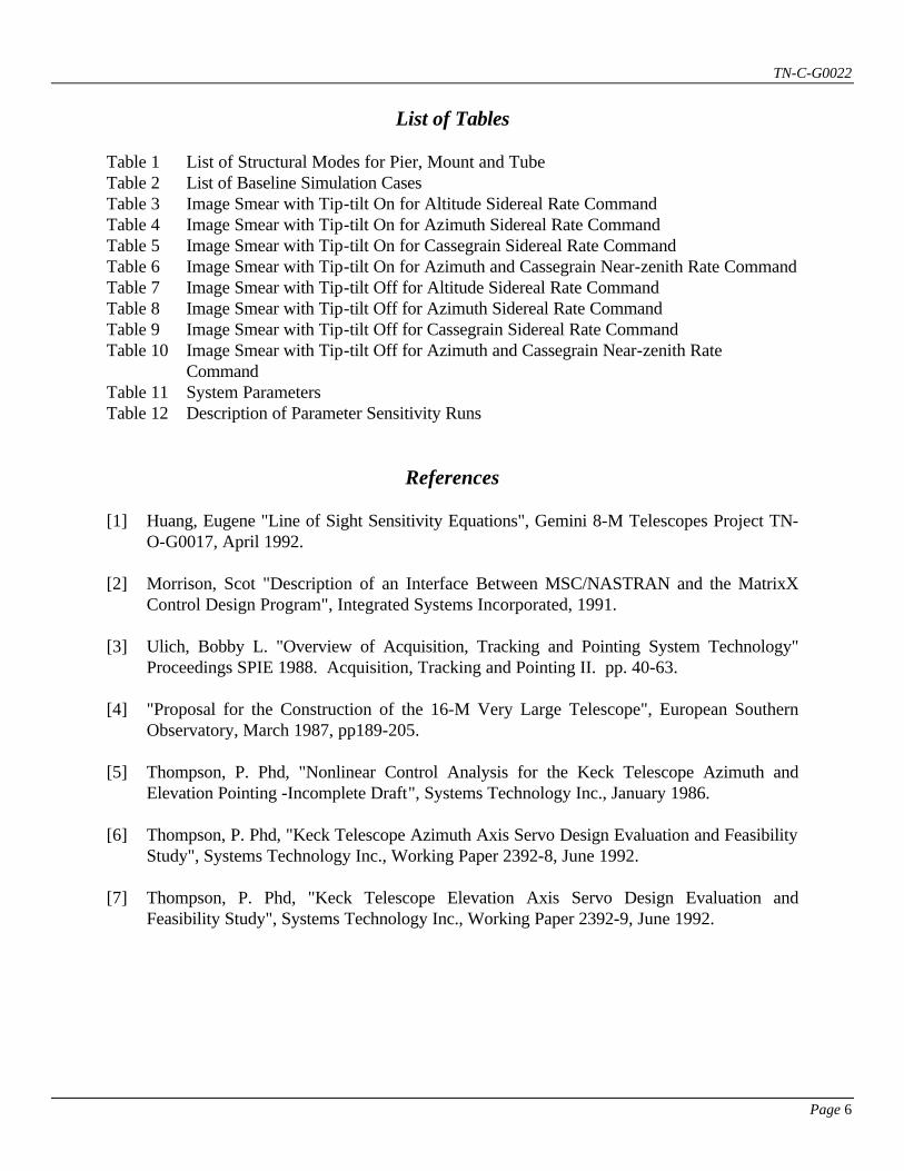
List of Tables Table 1 List of Structural Modes for Pier, Mount and Tube Table 2 List of Baseline Simulation Cases Table 3 Image Smear with Tip-tilt On for Altitude Sidereal Rate Command Table 4 Image Smear with Tip-tilt On for Azimuth Sidereal Rate Command Table 5 Image Smear with Tip-tilt On for Cassegrain Sidereal Rate Command Table 6 Image Smear with Tip-tilt On for Azimuth and Cassegrain Near-zenith Rate Command Table 7 Image Smear with Tip-tilt Off for Altitude Sidereal Rate Command Table 8 Image Smear with Tip-tilt Off for Azimuth Sidereal Rate Command Table 9 Image Smear with Tip-tilt Off for Cassegrain Sidereal Rate Command Table 10 Image Smear with Tip-tilt Off for Azimuth and Cassegrain Near-zenith Rate

Command Table 11 System Parameters Table 12 Description of Parameter Sensitivity Runs

References [1] Huang, Eugene "Line of Sight Sensitivity Equations", Gemini 8-M Telescopes Project TN-

O-G0017, April 1992. [2] Morrison, Scot "Description of an Interface Between MSC/NASTRAN and the MatrixX

Control Design Program", Integrated Systems Incorporated, 1991. [3] Ulich, Bobby L. "Overview of Acquisition, Tracking and Pointing System Technology"

Proceedings SPIE 1988. Acquisition, Tracking and Pointing II. pp. 40-63. [4] "Proposal for the Construction of the 16-M Very Large Telescope", European Southern

Observatory, March 1987, pp189-205. [5] Thompson, P. Phd, "Nonlinear Control Analysis for the Keck Telescope Azimuth and

Elevation Pointing -Incomplete Draft", Systems Technology Inc., January 1986. [6] Thompson, P. Phd, "Keck Telescope Azimuth Axis Servo Design Evaluation and Feasibility

Study", Systems Technology Inc., Working Paper 2392-8, June 1992. [7] Thompson, P. Phd, "Keck Telescope Elevation Axis Servo Design Evaluation and

Feasibility Study", Systems Technology Inc., Working Paper 2392-9, June 1992.

TN-C-G0022

Page 7

1.0 Summary The simulation shows that image smear estimate is 4.3e-8 radians RMS centroid motion (= 0.012 arcseconds increase in 50% encircled energy) for a baseline case of the altitude axis moving at sidereal rate. The parameters are included which are expected to cause the greatest degradation in image quality: encoder quantization, bearing friction, tip-tilt centroiding measurement noise, motor torque variation, tachometer error, drive eccentricity, and D/A motor command quantization. Section 2 describes the tracking simulation generally, including the assumed units, performance measure and axes. Section 3 gives the line of sight equations. Section 4 describes how the telescope structure is divided into sections labeled pier, mount, tube, cassegrain, and secondary mirror. Section 5 describes the drives and bearings that apply forces and torques to the free body structures of section 4. Section 6 describes some of the design trades used to find a reasonable control system gains. Section 7 describes the model verification efforts. Section 8 describes the conditions under which the simulation was run. Section 9 lists the results to date for the simulation, showing the RMS image smear relating to the various parameters for the input conditions described in section 8. Conclusions are listed in section 10, and section 11 describes some further areas of work. This report describes the simulation of the telescope structure and control system. Servo system related error sources are included, and the effect of the tip-tilt secondary mirror is quantified. Errors associated with the cassegrain rotator seem large and are rather uncertain, potentially leading to a significant performance risk.

TN-C-G0022

Page 8

2.0 Introduction The tracking simulation is a nonlinear 6 degree of freedom (6-DOF) time domain simulation which is meant to represent the interaction between the servo controls and the telescope structure. The six degrees of freedom are three translational dimensions, in meters, and three rotational dimensions, in radians. Other units are kilograms, seconds, Amperes and derived units such as Newtons for force and kg-m2 for rotational moment of inertia. The simulation is not meant to model those image smear error sources which are neither caused by nor affected by the servo system, including windshake, primary mirror seeing, and atmospheric effects. Line of sight (LOS) image motion is the metric by which performance is measured. The image equations take into account the motion of the focus, primary mirror pole, secondary mirror, and cassegrain rotator. The image equations produce line of sight errors in the two directions within the image plane labeled Tx and Ty. These image directions are respectively parallel and orthogonal to the altitude axis. Errors in the z-direction, that is along the optical axis, are not represented in this simulation. The LOS motion is usually represented as the root mean square (RMS or equivalent to standard deviation) error. The RMS errors are used for comparing to an error budget. Sometimes the time varying LOS error is used to produce a spectral density in order to show which system modes are contributing most to the RMS error. The image equations include the induced motion for a science object which is 509 microradians (=1.75 arcminutes, representing the edge of the science field) from the optical axis. The active secondary mirror is assumed to be tracking on an object which is 1750 microradians (=6.0 arcminutes, representing the edge of the guide field) from the optical axis. The error induced at the science object for fast tracking on a different object is modeled in the image equations and is more fully described in section 5.4 below with the description of the secondary mirror control system. The tracking simulation is made with the Matlab 4.0 software package running on a Pentium-60 type PC. It takes approximately 6 minutes of real time to run through 10 seconds of simulation time. There are approximately 320 states, with most of the states being used to model the structure of the telescope which has been divided into pier, mount and tube. The drives are modeled as lying between structural blocks, with any force applied to one part of the structure causing an equal and opposite reaction force against an adjoining part. Figure 2.1 shows the top level block diagram of the Matlab simulation. Note that this representation is hierarchical, with each block being composed of a number of sub-blocks, each of which can often be further reduced.

TN-C-G0022

Page 9

3.0 Line of Sight Image Equations The current equations used to represent motion in two dimensions of the image plane given as follows, from reference [1]. Rx(radians) = -2.0Rxp + 0.2584Rxs + 0.0694Typ - 0.0616Tys -0.0078Tyf Ry(radians) = 2.0Ryp - 0.2584Rys + 0.0694Txp - 0.0616Txs -0.0078Txf + Ry_cass where the T's on the right side represent translations in meters and the R's represent rotations in radians. The superscripts represent the axes either x or y. The subscripts represent primary, secondary, or focus positions. The error Ry_cass is due to the cassegrain tracking errors coupled to the use of an off-axis guide star, and is quantified in section 5.4 below.

TN-C-G0022

Page 10

4.0 Structures: Pier, Mount, Tube, Cassegrain, Secondary The structural blocks representing the pier, mount and tube have been supplied by the Gemini Telescope group and derived from a detailed finite element analysis (FEA) of the entire telescope using Nastran. The Nastran output is used to produce a state space representation of each block having the form &x = Ax + Bu y = Cx + Du where the x above represents the state vector, &x is the derivative, u is the vector of inputs and y is the vector of outputs. Each structural block may be thought of as representing a generalized mass having force (or torque) as an input and position (or angle) as an output. The structure blocks are generalized in the sense that each represents all six axes simultaneously, including some cross coupling between axes. Reference [2] describes the method used in the conversion from the FEA model to the state space model used in the tracking simulation. The drawings 4.1 through 4.5 were supplied by the Gemini Telescope group. Table 1 shows the list of modal frequencies in the pier, mount and tube structural blocks. The mount and tube each have 12 very low frequency modes which represent double integrators for each of the 6 degrees of freedom. These frequencies are small (around 1e-6) but non-zero because of the difficulty in the FEA program to represent pure integration. The pier block lacks the very low frequency modes because it is tied to ground; a constant force leads to a constant offset instead of a constant acceleration. One weakness of the transformation from FEA to state space model is that like inputs are all effectively tied together. For example if an azimuth torque is applied to the mount, this is modeled as divided equally among the 4 azimuth drives. Therefore no differential motor torques may be represented in the simulation. Similarly all like outputs are summed to produce the measured rotation in the z direction. This weakness is in the application and is not expected to cause a large impact on the results, since in normal operation the differential motor torques would be expected to be much smaller than the common mode motor torques. The method could be expanded to include all of the motors and bearings acting independently, but at the expense of a manyfold increase in complexity and runtime. 4.1 Pier Figure 4.1 shows a stylized drawing of the pier showing the locations of bearing and drive motor contact points. The model included in the simulation represents the mass, compliance, and damping of the telescope pier together with some compliances and dampings which tie it to ground (earth). The pier is tied to the mount block by way of the azimuth drive. The motor forces are distributed over 4 points, all of which are equal magnitude and always in phase as

TN-C-G0022

Page 11

described earlier. The bearing frictional forces are distributed over 6 points and these are in phase as well, though the bearing forces may be out of phase with the motor forces. The line representing the signal path into the pier block is composed of 12 forces and torques, the first 6 for the motor and the latter 6 for the bearing. The input vector is formed from augmenting the two 6-vectors as shown:

u

xy

y

xyz

xyz

=

direction motor forcedirection motor force

z direction motor forcex axis motor torque

axis motor torquez axis motor torquedirection bearing forcedirection bearing forcedirection bearing force

axis bearing torqueaxis bearing torqueaxis bearing torque

Similarly the output of the pier follows the same convention with forces being replaced by positions and torques being replaced by angles. Throughout the simulation, the x axis is along the altitude axis, the z axis is toward zenith, and the y axis is orthogonal to both of these to form a right-hand coordinate system (x cross y equals z). 4.2 Mount A drawing of the mount structure is shown in Figure 4.2. The mount model has two input signal lines and two output signal lines, where each line is a 12-vector following the same convention described for the pier. The two signal lines represent the forces due to the azimuth and altitude drives. The two output signal lines represent the corresponding positions and angles as measured at the motors and bearings. The mount block is attached to the tube block through the altitude drive. 4.3 Tube The tube structural block is the most complicated of all of the blocks of Figure 2.1 in that it contains the most state variables. Figure 4.3 shows the tube structure. The model is made up of 118 states, representing the most important 59 modes of the telescope model. These modes are the most important in the sense that they contribute the largest amount to the outputs. It interfaces to the mount block by way of the altitude drive. There are two smaller structures

TN-C-G0022

Page 12

attached to the tube, representing the secondary mirror and the cassegrain instrument with their respective drives. The tube model also has two other 6-vectors for outputs, representing the focus and primary mirror pole. These last two outputs are used in the image equations. Included as part of the tube is the primary mirror and its supports. The model has 6 vertical and 4 lateral supports arranged symmetrically. 4.4 Cassegrain A drawing of the cassegrain rotator is shown in the lower portion of Figure 4.4. The model for the cassegrain instrument is quite simple, consisting of only 3 masses and 3 moments of inertia with no cross coupling between axes. Since each of the 6 axes requires 2 states, the cassegrain model has a net 12 states. It interfaces to the tube through the cassegrain drive. The known low frequency modes of the cassegrain instrument/drive assembly are represented in the model for the cassegrain drive, described in section 5.3 below. 4.5 Secondary Mirror A drawing of the secondary support structure is shown in Figure 4.5. The secondary support structure model, like the cassegrain instrument described above, contains only 12 states. No flexural modes are represented for the mirror itself, although the drive described in section 5.4 below contains spring constants and damping to model the structure mounting the secondary support structure to the tube. The secondary mirror is relatively free to rotate in the x and y directions, and relatively stiff for z rotation and all of the translations. The rotation about the x and y axes is used to effect the tip/tilt correction.

TN-C-G0022

Page 13

5.0 Drives and bearings There are four drive blocks, one each for azimuth, altitude, cassegrain, and secondary mirror. These blocks typically model a motor in one free axis of rotation and a spring-damper pair for the other non-free axes. Additionally, the drive blocks contain bearing friction about the free axis. Each of the four drive blocks are described in detail in the following sections of this report. The bearing friction model has been supplied by Kaman Aerospace corporation, and includes three types of friction: viscous, coulomb, and stiction. Viscous friction, sometimes called linear friction, consists of a force which is proportional to velocity. Coulomb friction is a torque which is constant at all velocities. Stiction is a torque which is larger than coulomb friction and present only at tiny velocities. The transition from stiction to Coulomb friction is modeled with a 4th order polynomial to match curves given by Kaman. The transition region from high stiction to lower Coulomb friction has an important effect upon stability, because there is effectively a region of negative damping where increasing speed decreases friction. This negative damping can cause instability or a large limit cycle if not properly taken into account. The axes which are not considered free to rotate must be tied together somehow so that a movement in one structure transmits that movement to an adjacent structure. One possible way would be tie the points together and not permit any deviation. Unfortunately, this would lead to infinitely high frequency structural modes, which would be impossible to simulate. Instead, it has been chosen to tie together the corresponding points on adjacent structures by way of very stiff spring-damper pairs. The stiffness of the springs are chosen to give a natural mode which is fast compared to other system modes so as not to change the overall character of the structural oscillations. The stiffnesses are chosen to be sufficiently slow so as to be modelable within the simulation given a reasonable amount of runtime. Figure 5.1 helps to illustrate how the springs and dampers are chosen for those axes which are to remain relatively fixed. This simple case shows only one translational axis, but the results easily extend to the rotational axes. Two masses are shown separated by a distance x. A force labeled F acts upon both of the masses equally and in opposite directions. The net acceleration will be the sum of the accelerations for the two masses: && / / ( / / )x F M F M F M M= + = +1 2 1 1 1 2 The force will be considered to be supplied by the sum of a spring and a damper. The spring force is proportional to the distance with gain KS, and the damper force is proportional to the velocity with gain KD. Substituting the force into the equation above gives && ( / / )( * * &)x M M KS x KD x= + − −1 1 1 2 Replacing derivatives with the operator S gives the characteristic equation: s2 + s*(1/M1 + 1/M2)*KD + (1/M1 + 1/M2)*KS = 0

TN-C-G0022

Page 14

Compare this to a desired characteristic second-order equation with damping z and natural frequency w(rad/sec) : s2 + s*2zw + w2 = 0. The coefficients of the above two equations may be compared to solve for the spring and damper gains given the natural frequency and damping:

( )( )

KS wM MM M

KDzwM MM M

=+

=+

2 1 21 2

2 1 21 2

**

For most of the non-free axes the damping was chosen to be 3% and the natural frequency was chosen to be 500 rad/sec. The low damping is consistent with the rest of the structure and the high natural frequency is used to avoid introducing any other low-frequency modes into the system. The KS and KD for the various axes of the cassegrain drive were not chosen by the above method but rather were supplied by the instrument group. The FEA model developed by the telescope group does not have the couplings described above. Instead, the FEA model is entirely one piece. The couplings described above are necessary because the FEA model has been bisected to give the state space model used in the servo simulation described in this paper. The bisection process produces 2 nodes where there was only one before. It is necessary to join these 2 nodes with springs and dampers as described, and it is hoped that the resulting natural frequencies are sufficiently high (i.e. 500 rad/sec) to go unnoticed in the simulation. 5.1 Azimuth Drive Figure 5.1 shows a breakdown of the azimuth drive block. There are two 12-vectors input and one 12-vector output. The first input vector represents the positions seen by motor and bearing on the pier side and the second input vector represents the positions seen by the motor and bearing on the mount side. The motor primarily acts upon the z rotation. The oil bearing model provides torques that resist z rotation based on the frictional model. The oil bearing as modeled provides no translational forces in the x or y directions, but is stiff in the z translation as well as x and y rotations. The x and y translations are taken up by radial springs. The difference between the pier and mount z rotations in Figure 5.1 is measured by way of a resolver which is modeled as a quantizer. The output of the quantizer is compared to an azimuth command and applied to the azimuth controller block of Figure 5.1.2. The measured angle and command are acted upon by a digital controller to produce a commanded motor velocity, which passes through a DA converter (modeled as another quantizer) and becomes an analog motor command. The motor produces a torque which is the output of Figure 5.1.2.3. This structure of the controller can be thought of as a fast analog velocity inner-loop embedded within a slower

TN-C-G0022

Page 15

digital position outer-loop consisting of a PI (proportional-integral) controller and velocity feed-forward. The same structure was chosen by the VLT as described in their simulation report, reference [4]. The same structure was also chosen by the Keck telescope as described their reports, references [5] through [7]. Figure 5.1.2.2 shows how the digital controller is broken down into three parts: an acceleration controller a velocity controller and a linear controller. Only one of the three controllers is active at any time, as determined by the switching logic. For very small errors, such as would exist during tracking, the switching logic chooses the linear controller which is effectively a PI (proportional-integral) type controller with the addition of velocity feed-forward. When there is a large error between the commanded angle and achieved, for example during slewing, the switching logic chooses the acceleration controller until velocity is near the specified maximum then activates the velocity controller to hold the maximum velocity until it is time to begin deceleration. The switching logic then activates the acceleration controller to give the maximum allowable deceleration. Finally, when the error and rate are both small, the switching logic activates the linear controller in order to smoothly transition back into tracking. The analog motor model of Figure 5.1.2.3 was suggested by Kaman Aerospace. The analog motor rate command input is compared to the measured motor rate coming from a tachometer to produce a rate error which in fact will be a voltage. The rate error passes through a velocity compensation filter. This filter is effectively a lead-lag chosen to give acceptable stability margins and bandwidth. The output of the lead-lag filter is a voltage command to the motor and there is a power amplifier implied. The commanded voltage minus a back-emf voltage is available for providing motor torque. All motors are modeled as seeing the same voltage, and the gain labeled v2torq converts the voltage command to one motor into the sum of torques supplied by all four motors working together. The net torque is multiplied by the drive ratio to obtain the torque which is applied to the bottom of the mount structure. 5.2 Altitude Drive The altitude drive block of Figure 5.2 is analogous with the azimuth drive described in the previous section, with the only changes being in some specific coefficient values and the effected axes. The altitude drive causes x-rotation of the tube with respect to the mount, whereas the azimuth drive causes z-rotation of the mount with respect to the pier. 5.3 Cassegrain Drive In the top level simulation diagram, Figure 5.3, the cassegrain block contains both the cassegrain drive and the cassegrain structure. The cassegrain drive is analogous to the azimuth drive described in section 5.1 above, with some coefficients changed and the addition of an explicit model of the coupling between motor shaft and driven load. This coupling is not shown on the azimuth or altitude axes because it is implicit to the mount and tube models respectively. The z axis is controlled to de-rotate the image plane, with rates ranging from 0 to 0.009 rad/sec (0.5 deg/sec).

TN-C-G0022

Page 16

The analog motor loop is similar to the loop for azimuth, described in section 5.1, with the addition of the motor moment of inertia. The motor torque minus a back torque, caused by reacting against the telescope structure, goes toward accelerating the motor moment of inertia and is integrated to become the motor shaft position angle. The motor position is output from the analog motor block. The drive mechanism including the drive ratio and compliance is modeled in Figure 5.3.2.4. The spring constant was chosen by the Gemini Instrument group based on manufacturers specification for the gearbox stiffness. The damper was chosen to give a damping of 0.03 based on the calculations described in section 5.0 above. 5.4 Secondary Drive Figure 5.4 shows how the secondary block is broken down into the secondary drive and the secondary support structure. The secondary mirror may be thought of as being mounted on springs, with no sliding bearings, and therefore it lacks the bearing friction described for the previous drives. The secondary mirror is relatively easy to rotate about the x and y axes, since there are only light springs attached to the active optics actuators. These two axes are modeled in the secondary drive, Figure 5.4.1, having a 6.4Hz resonant frequency with a damping of 3%. When tip-tilt is activated, the resonant frequency is increased and the damping is improved electronically. Figure 5.4.1.1 shows the tip-tilt controller. There are in effect two controllers, one for each axis. Each controller is third order, having 3 poles and 3 zeros. One of the poles is placed at the origin (i.e. there is a pure integration) in order to be able to remove steady state errors. The other coefficients are chosen to achieve a 4th order Butterworth closed-loop pole configuration. The closed loop bandwidth was chosen to be 25Hz subject to the requirement that sampling rate should not exceed 200Hz. The sampling rate must be around 8 times the bandwidth in this case because of the destabilizing effect of the relatively large delays associated with the CCD integration and numerical processing. The CCD integration time is 5ms, for an average delay of 2.5 ms, and the processing time is 0.5 ms. The tip-tilt controller includes a centroid measurement noise error, modeled here as a white noise source passed through a low pass filter. The RMS of the noise source at 200Hz sampling is obtained from reference [3]. Since the simulation runs at 1000Hz and the digitized tip-tilt controller will run at 200Hz, it is necessary to apply a scale factor of sqrt(5) to the simulation. A scale factor of sqrt(0.5) is also included to model the noise in one axis rather than both axes simultaneously. The low pass filter on the noise source is meant to approximate the inverse sinc-squared effect which is known to result from sampling the noise at 200Hz. Figure 5.10 shows the negative effect tip-tilt control can have on errors in the field rotation. A guide star, labeled g, is 6 arcminutes from the optical axis in the x direction. The science object, labeled s, is 1.75 arcminutes from the optical axis in the negative x direction. A tracking error, for example due to the cassegrain rotator, causes the field to be rotated an amount labeled rz_err. Then the guide star moves in the negative y direction to the new position labeled g'. This would

TN-C-G0022

Page 17

cause the tip-tilt controller to move in the negative y direction by the same amount, which is in the opposite direction and greater magnitude than the compensation required to keep the science object centered. The total error introduced by the combination of tip-tilt with a cassegrain tracking error will be the sum of the errors at the science object and the guide object. Each error may be calculated by using the approximation x=sin(x) to represent the errors as the moment arm times the field rotation error: ry_cass(arcmin) = 1.75arcmin * rz_err(rad) + 6.0 arcmin * rzerr(rad) ry_cass(arcmin) = 7.75 arcmin * rz_err(rad) ry_cass(rad) = 0.00225(rad) * rz_err(rad) So for example if the cassegrain tracking error is one quantization step for the cassegrain encoder, rz_err= 4.9e-6 and the resulting image plane error will be 0.00225*4.9e-6 = 1.1e-8 rad. In reality it will likely be difficult to keep the cassegrain axis tracking to within one encoder count in the presence of friction, so the cassegrain induced error will be greater than this estimate. The conditions described above are conservative in that the guide star is at the edge of the guide field and the science object is at the edge of the science field, and the two objects are on opposite sides of the optical axis. If the field of view had been translated instead of rotated, then the guide star would have moved the same as the science object and the tip-tilt correction would be correct. So tip-tilt control attenuates field translations and worsens or accentuates field rotations. A separate and much simplified simulation is used to evaluate the effect of the tip-tilt controller upon image smear due to windshake. The justification for this is that the secondary mirror is small compared to the rest of the telescope, and the torques reflected back into the system will cause very little motion. The telescope group supplied spectra of uncompensated image smear due to windshake for a number of different conditions. These spectra were operated upon by a closed loop system modeling the secondary mirror with supports and a controller with sampling. The sampling degrades performance due to the added delay. Appendix A36 describes the latest tip-tilt compensation for windshake.

TN-C-G0022

Page 18

6.0 Design Trades There were a number of somewhat arbitrary assumptions that went into creating the tracking simulation. It was necessary to chose controllers for azimuth, altitude and cassegrain. So the gains and filters were somewhat arbitrarily chosen. It was also necessary to chose motor compensation filters as part of the analog motor controllers. The non-arbitrary physical parameters of the system are listed in Table 11 for reference. Figure 6.1 shows the step response of the azimuth control loop subject to a 5 arcsecond (2.4e-5 radian) command input. The PI gains of the controller, Figure 5.1.2.2.4, were chosen such that the step response would have a settling time (defined as to within 10% of final value) of about 1 second. The velocity compensation lead-lag filter of Figure 5.1.2.3 was chosen based upon Bode plot analysis to give the best gain and phase margins. This figure has considerable overshoot because the step size is outside the range of what can be handled by the purely linear controller. The acceleration controller causes a relatively large overshoot for this small move. Protecting the acceleration limit of the azimuth axis forces the controller to leave the purely linear region, which increases the settling time. Calculations show that the purely linear region should exist for steps less than about 2 arcseconds. Increasing the azimuth acceleration limit will reduce the time required to a step, under the conditions when it is acceleration limited, but it is not known by how much. The azimuth response compares somewhat closely to the Keck results of reference [6], which shows the response to a step settling to 10% about 0.7 second. Figure 6.2 shows the step response for the altitude control loop subject to a 5 arcsecond (2.4e-5 radian) command, subject to the same 1 second settling time. The altitude response is faster and smoother than that obtained for the azimuth of figure 6.1 because the dynamics of the mount cause more phase lag at lower frequencies than do the dynamics of the tube. The azimuth controller could be improved by building a more complex controller which had more information about the dynamics of the plant which it is controlling. The danger in building this into the servo model is that it could lead to overly-optimistic results as a controller is tailored to the exact structure. The Keck report, reference [7] shows a 5% settling time of 0.96 seconds, or 10% in about 0.9 seconds. Figure 6.3 shows the step response for the cassegrain control loop. A larger stepsize (1mrad) was chosen for the cassegrain controller than for the azimuth or altitude described above because the cassegrain has a much coarser encoder resolution. A very small step, on the order of a few encoder counts, would show more overshoot and longer settling because of the effective lag introduced by the encoder. The system would come to rest with approximately 1 encoder count of error. For the step size used, the 10% settling time is about 0.7 seconds. It should be noted that performance will depend somewhat upon the speed of response, or bandwidth, of the servo loops described above. A higher bandwidth loop will do better at rejecting disturbances but might permit more measurement noise to pass through the system. Conversely, a slower system will be more tolerant of measurement noise, but be unable to quickly track out disturbances. So it might be worth spending some time on future work to optimize the

TN-C-G0022

Page 19

digital controller and the analog velocity compensation of Figures 5.1.2.2.4 and 5.1.2.3, subject to the mix of error sources that are present.

TN-C-G0022

Page 20

7.0 Model Verification This chapter describes the work done to evaluate the telescope model and verify its resemblance to reality. With no actual hardware yet built, the problem was knowing what to verify the model against. The mechanics of the model are based upon transformations from a Finite Element Analysis (F.E.A.) model to state-space models. If any discrepancy occurs, it is likely to be with these transformations. Therefore a separate, much simpler, model was built. This used the more conventional method of inertia's coupled by compliance. This model is not as accurate as the main model as it does not take into account nonfree axis movement and does not model as many structural modes. However, the simpler model acts as a yardstick to determine the realism of the main model. Another potential problem with the main model was the derivation of the tacho signals. The main model has no pure velocity signals and therefore tacho feedback is derived by differentiating position signals. It was intended to use the yardstick model to investigate the effect of doing this. The work was divided into four sections • Dissection of main model into its component parts (i.e. Altitude drive, Azimuth drive and

Cassegrain rotator). • Construction of a yardstick model for each of the main model dissections. • Derivation of parameters for the yardstick models. • Comparison of models and tacho derivation investigation. The following sub-sections describe each of these four bits of work in detail. 7.1 Model Dissection There were two reasons for dissecting the main model • Each yardstick could be compared against it's equivalent part of the main model. • Simulation was faster.

Fig 7.1 shows the way in which-the main model was dissected into four. 7.1.1 Azimuth Dissection This dissection consists of the three blocks - Pier, Az dr and Mount. This is effectively a model of the telescope without a tube fitted. Hence the signal representing force reaction from the altitude drive is zero. 7.1.2 Altitude Dissection This dissection consists of three blocks - Mount, Alt dr and Tube. The azimuth drive was considered to be stationary and fixed to ground. To represent this the mount block needed to be

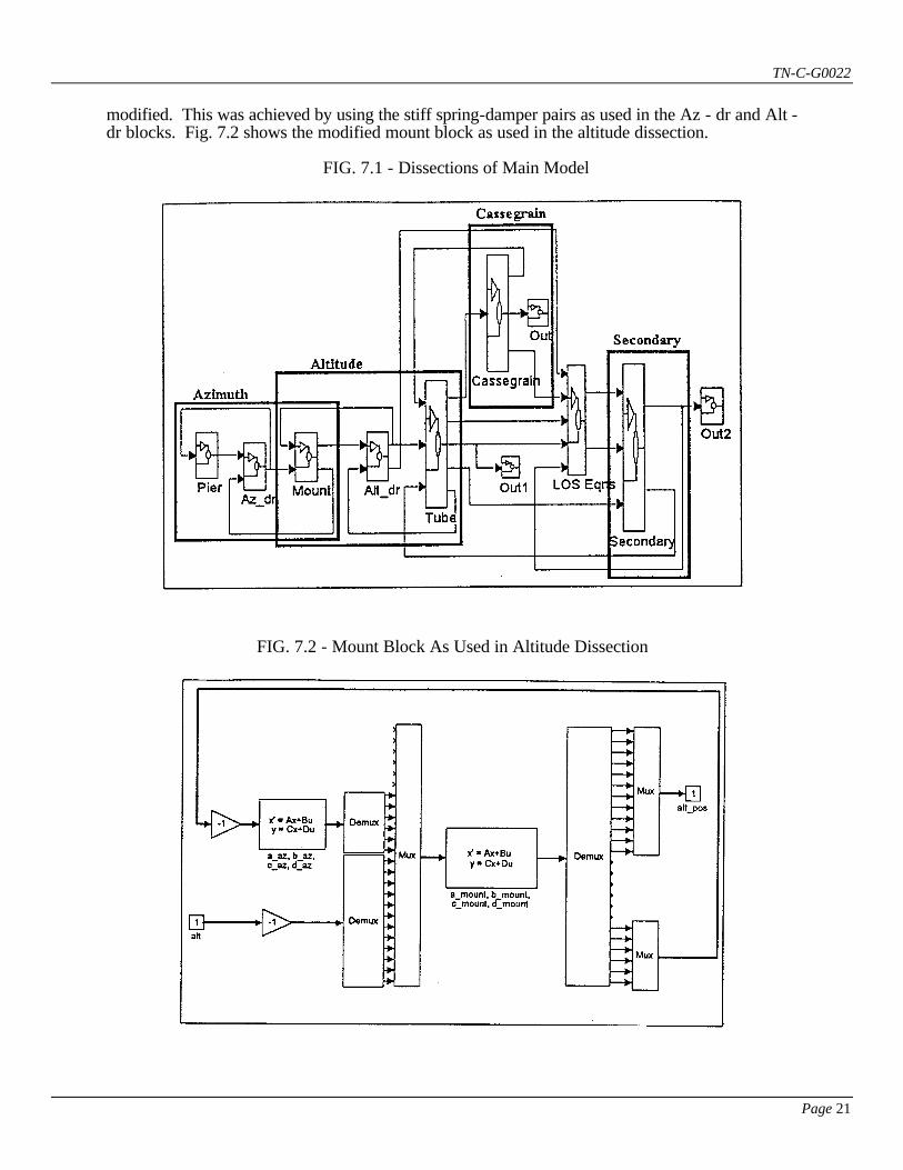
TN-C-G0022

Page 21

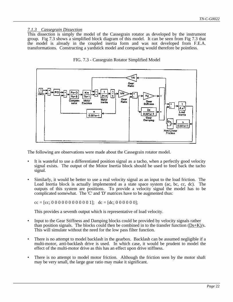
modified. This was achieved by using the stiff spring-damper pairs as used in the Az - dr and Alt - dr blocks. Fig. 7.2 shows the modified mount block as used in the altitude dissection.

FIG. 7.1 - Dissections of Main Model

FIG. 7.2 - Mount Block As Used in Altitude Dissection

TN-C-G0022

Page 22

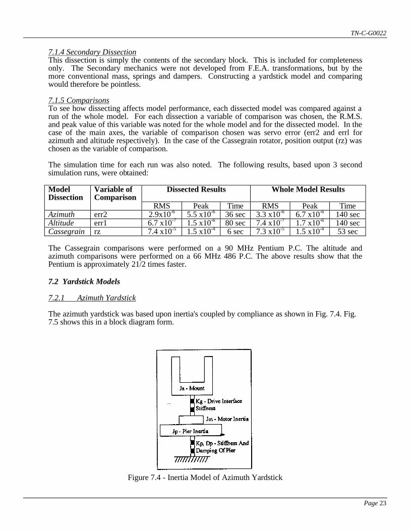
7.1.3 Cassegrain Dissection This dissection is simply the model of the Cassegrain rotator as developed by the instrument group. Fig 7.3 shows a simplified block diagram of this model. It can be seen from Fig 7.3 that the model is already in the coupled inertia form and was not developed from F.E.A. transformations. Constructing a yardstick model and comparing would therefore be pointless.

The following are observations were made about the Cassegrain rotator model. • It is wasteful to use a differentiated position signal as a tacho, when a perfectly good velocity

signal exists. The output of the Motor Inertia block should be used to feed back the tacho signal.

• Similarly, it would be better to use a real velocity signal as an input to the load friction. The

Load Inertia block is actually implemented as a state space system (ac, bc, cc, dc). The outputs of this system are positions. To provide a velocity signal the model has to be complicated somewhat. The 'C' and 'D' matrices have to be augmented thus:

cc = [cc; 0 0 0 0 0 0 0 0 0 0 0 1]; dc = [dc; 0 0 0 0 0 0]; This provides a seventh output which is representative of load velocity. • Input to the Gear Stiffness and Damping blocks could be provided by velocity signals rather

than position signals. The blocks could then be combined in to the transfer function (Ds+K)/s. This will simulate without the need for the low pass filter function.

• There is no attempt to model backlash in the gearbox. Backlash can be assumed negligible if a

multi-motor, anti-backlash drive is used. In which case, it would be prudent to model the effect of the multi-motor drive as this has an effect upon drive stiffness.

• There is no attempt to model motor friction. Although the friction seen by the motor shaft

may be very small, the large gear ratio may make it significant.

FIG. 7.3 - Cassegrain Rotator Simplified Model

TN-C-G0022

Page 23

7.1.4 Secondary Dissection This dissection is simply the contents of the secondary block. This is included for completeness only. The Secondary mechanics were not developed from F.E.A. transformations, but by the more conventional mass, springs and dampers. Constructing a yardstick model and comparing would therefore be pointless. 7.1.5 Comparisons To see how dissecting affects model performance, each dissected model was compared against a run of the whole model. For each dissection a variable of comparison was chosen, the R.M.S. and peak value of this variable was noted for the whole model and for the dissected model. In the case of the main axes, the variable of comparison chosen was servo error (err2 and errl for azimuth and altitude respectively). In the case of the Cassegrain rotator, position output (rz) was chosen as the variable of comparison. The simulation time for each run was also noted. The following results, based upon 3 second simulation runs, were obtained: Model Dissection

Variable of Comparison

Dissected Results

Whole Model Results

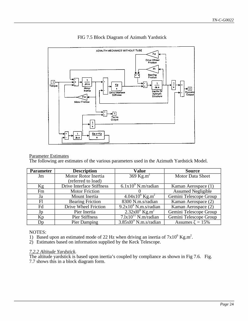
RMS Peak Time RMS Peak Time Azimuth err2 2.9x10-6 5.5 x10-6 36 sec 3.3 x10-6 6.7 x10-6 140 sec Altitude err1 6.7 x10-7 1.5 x10-6 80 sec 7.4 x10-7 1.7 x10-6 140 sec Cassegrain rz 7.4 x10-5 1.5 x10-4 6 sec 7.3 x10-5 1.5 x10-4 53 sec The Cassegrain comparisons were performed on a 90 MHz Pentium P.C. The altitude and azimuth comparisons were performed on a 66 MHz 486 P.C. The above results show that the Pentium is approximately 21/2 times faster. 7.2 Yardstick Models 7.2.1 Azimuth Yardstick The azimuth yardstick was based upon inertia's coupled by compliance as shown in Fig. 7.4. Fig. 7.5 shows this in a block diagram form.

Figure 7.4 - Inertia Model of Azimuth Yardstick

TN-C-G0022

Page 24

Parameter Estimates The following are estimates of the various parameters used in the Azimuth Yardstick Model. Parameter Description Value Source

Jm Motor Rotor Inertia (referred to load)

369 Kg.m2 Motor Data Sheet

Kg Drive Interface Stiffness 6.1x109 N.m/radian Kaman Aerospace (1) Fm Motor Friction 0 Assumed Negligible Ja Mount Inertia 4.04x106 Kg.m2 Gemini Telescope Group Fl Bearing Friction 8300 N.m.s/radian Kaman Aerospace (2) Fd Drive Wheel Friction 9.2x104 N.m.s/radian Kaman Aerospace (2) Jp Pier Inertia 2.32xl08 Kg.m2 Gemini Telescope Group Kp Pier Stiffness 7.lx1011 N.m/radian Gemini Telescope Group Dp Pier Damping 3.85xl09 N.m.s/radian Assumes ζ = 15%

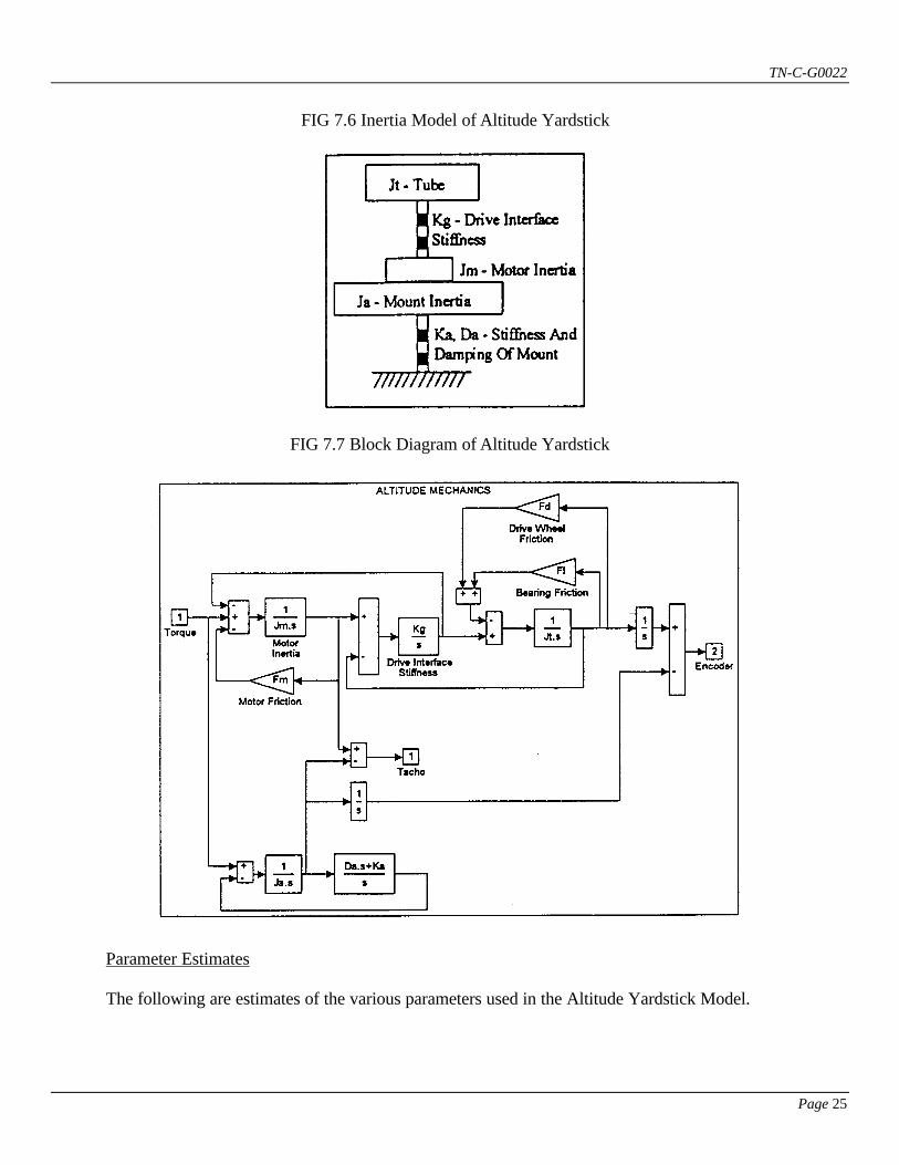
NOTES: 1) Based upon an estimated mode of 22 Hz when driving an inertia of 7x106 Kg.m2. 2) Estimates based on information supplied by the Keck Telescope. 7.2.2 Altitude Yardstick. The altitude yardstick is based upon inertia’s coupled by compliance as shown in Fig 7.6. Fig. 7.7 shows this in a block diagram form.

FIG 7.5 Block Diagram of Azimuth Yardstick

TN-C-G0022

Page 25

Parameter Estimates

The following are estimates of the various parameters used in the Altitude Yardstick Model.

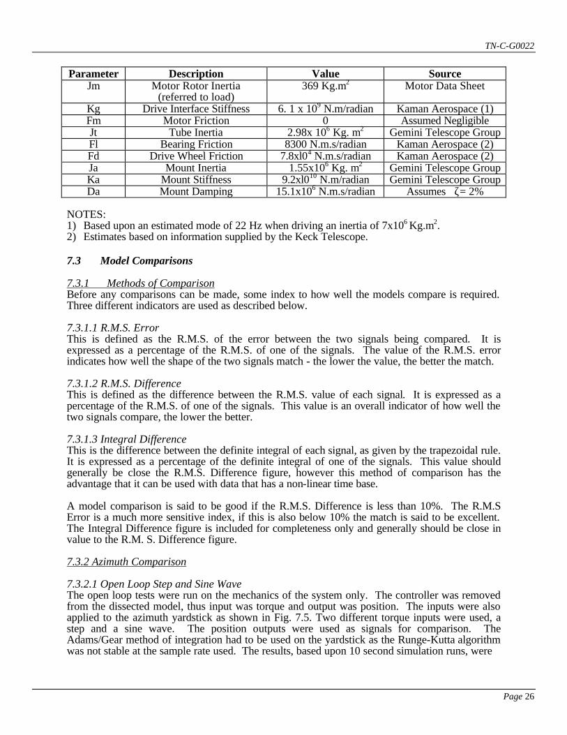
FIG 7.6 Inertia Model of Altitude Yardstick

FIG 7.7 Block Diagram of Altitude Yardstick

TN-C-G0022

Page 26

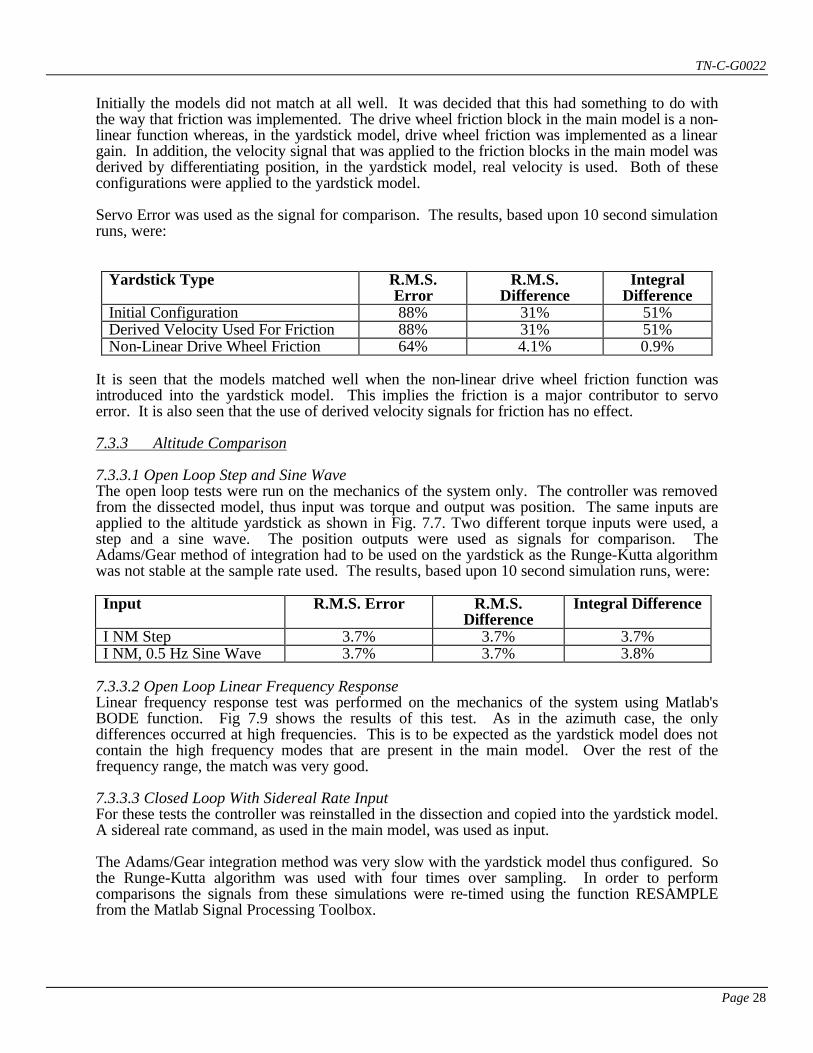
Parameter Description Value Source Jm Motor Rotor Inertia

(referred to load) 369 Kg.m2 Motor Data Sheet

Kg Drive Interface Stiffness 6. 1 x 109 N.m/radian Kaman Aerospace (1) Fm Motor Friction 0 Assumed Negligible Jt Tube Inertia 2.98x 106 Kg. m2 Gemini Telescope Group Fl Bearing Friction 8300 N.m.s/radian Kaman Aerospace (2) Fd Drive Wheel Friction 7.8xl04 N.m.s/radian Kaman Aerospace (2) Ja Mount Inertia 1.55x106 Kg. m2 Gemini Telescope Group Ka Mount Stiffness 9.2xl010 N.m/radian Gemini Telescope Group Da Mount Damping 15.1x106 N.m.s/radian Assumes ζ= 2%

NOTES: 1) Based upon an estimated mode of 22 Hz when driving an inertia of 7x106 Kg.m2. 2) Estimates based on information supplied by the Keck Telescope. 7.3 Model Comparisons 7.3.1 Methods of Comparison Before any comparisons can be made, some index to how well the models compare is required. Three different indicators are used as described below. 7.3.1.1 R.M.S. Error This is defined as the R.M.S. of the error between the two signals being compared. It is expressed as a percentage of the R.M.S. of one of the signals. The value of the R.M.S. error indicates how well the shape of the two signals match - the lower the value, the better the match. 7.3.1.2 R.M.S. Difference This is defined as the difference between the R.M.S. value of each signal. It is expressed as a percentage of the R.M.S. of one of the signals. This value is an overall indicator of how well the two signals compare, the lower the better. 7.3.1.3 Integral Difference This is the difference between the definite integral of each signal, as given by the trapezoidal rule. It is expressed as a percentage of the definite integral of one of the signals. This value should generally be close the R.M.S. Difference figure, however this method of comparison has the advantage that it can be used with data that has a non-linear time base. A model comparison is said to be good if the R.M.S. Difference is less than 10%. The R.M.S Error is a much more sensitive index, if this is also below 10% the match is said to be excellent. The Integral Difference figure is included for completeness only and generally should be close in value to the R.M. S. Difference figure. 7.3.2 Azimuth Comparison 7.3.2.1 Open Loop Step and Sine Wave The open loop tests were run on the mechanics of the system only. The controller was removed from the dissected model, thus input was torque and output was position. The inputs were also applied to the azimuth yardstick as shown in Fig. 7.5. Two different torque inputs were used, a step and a sine wave. The position outputs were used as signals for comparison. The Adams/Gear method of integration had to be used on the yardstick as the Runge-Kutta algorithm was not stable at the sample rate used. The results, based upon 10 second simulation runs, were

TN-C-G0022

Page 27

Input R.M.S. Error R.M.S. Difference Integral Difference I NM Step 1.4% 1.4% 1.4%

1 NK 0.5 Hz Sine Wave 1.6% 1.6% 1.5%

It can be seen that the agreement between the models was excellent.

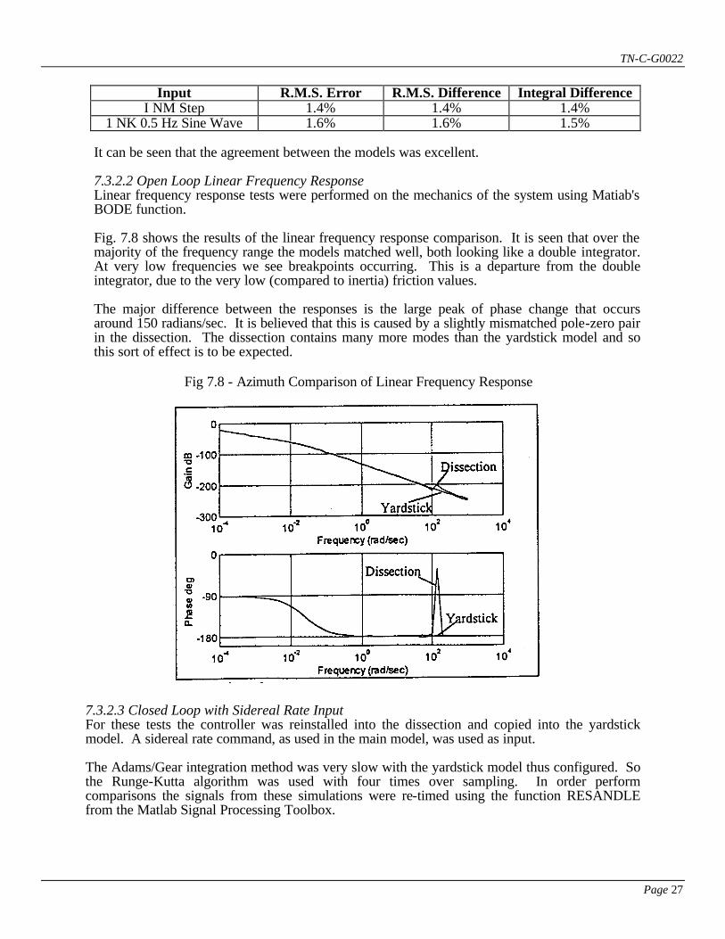
7.3.2.2 Open Loop Linear Frequency Response Linear frequency response tests were performed on the mechanics of the system using Matiab's BODE function.

Fig. 7.8 shows the results of the linear frequency response comparison. It is seen that over the majority of the frequency range the models matched well, both looking like a double integrator. At very low frequencies we see breakpoints occurring. This is a departure from the double integrator, due to the very low (compared to inertia) friction values.

The major difference between the responses is the large peak of phase change that occurs around 150 radians/sec. It is believed that this is caused by a slightly mismatched pole-zero pair in the dissection. The dissection contains many more modes than the yardstick model and so this sort of effect is to be expected.

7.3.2.3 Closed Loop with Sidereal Rate Input For these tests the controller was reinstalled into the dissection and copied into the yardstick model. A sidereal rate command, as used in the main model, was used as input. The Adams/Gear integration method was very slow with the yardstick model thus configured. So the Runge-Kutta algorithm was used with four times over sampling. In order perform comparisons the signals from these simulations were re-timed using the function RESANDLE from the Matlab Signal Processing Toolbox.

Fig 7.8 - Azimuth Comparison of Linear Frequency Response

TN-C-G0022

Page 28

Initially the models did not match at all well. It was decided that this had something to do with the way that friction was implemented. The drive wheel friction block in the main model is a non-linear function whereas, in the yardstick model, drive wheel friction was implemented as a linear gain. In addition, the velocity signal that was applied to the friction blocks in the main model was derived by differentiating position, in the yardstick model, real velocity is used. Both of these configurations were applied to the yardstick model. Servo Error was used as the signal for comparison. The results, based upon 10 second simulation runs, were:

Yardstick Type R.M.S. Error

R.M.S. Difference

Integral Difference

Initial Configuration 88% 31% 51% Derived Velocity Used For Friction 88% 31% 51% Non-Linear Drive Wheel Friction 64% 4.1% 0.9%

It is seen that the models matched well when the non-linear drive wheel friction function was introduced into the yardstick model. This implies the friction is a major contributor to servo error. It is also seen that the use of derived velocity signals for friction has no effect. 7.3.3 Altitude Comparison 7.3.3.1 Open Loop Step and Sine Wave The open loop tests were run on the mechanics of the system only. The controller was removed from the dissected model, thus input was torque and output was position. The same inputs are applied to the altitude yardstick as shown in Fig. 7.7. Two different torque inputs were used, a step and a sine wave. The position outputs were used as signals for comparison. The Adams/Gear method of integration had to be used on the yardstick as the Runge-Kutta algorithm was not stable at the sample rate used. The results, based upon 10 second simulation runs, were: Input R.M.S. Error R.M.S.

Difference Integral Difference

I NM Step 3.7% 3.7% 3.7% I NM, 0.5 Hz Sine Wave 3.7% 3.7% 3.8%

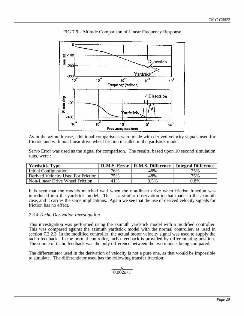
7.3.3.2 Open Loop Linear Frequency Response Linear frequency response test was performed on the mechanics of the system using Matlab's BODE function. Fig 7.9 shows the results of this test. As in the azimuth case, the only differences occurred at high frequencies. This is to be expected as the yardstick model does not contain the high frequency modes that are present in the main model. Over the rest of the frequency range, the match was very good. 7.3.3.3 Closed Loop With Sidereal Rate Input For these tests the controller was reinstalled in the dissection and copied into the yardstick model. A sidereal rate command, as used in the main model, was used as input. The Adams/Gear integration method was very slow with the yardstick model thus configured. So the Runge-Kutta algorithm was used with four times over sampling. In order to perform comparisons the signals from these simulations were re-timed using the function RESAMPLE from the Matlab Signal Processing Toolbox.

TN-C-G0022

Page 29

As in the azimuth case, additional comparisons were made with derived velocity signals used for friction and with non-linear drive wheel friction installed in the yardstick model. Servo Error was used as the signal for comparison. The results, based upon 10 second simulation runs, were : Yardstick Type R-M.S. Error R-M.S. Difference Integral Difference Initial Configuration 76% 48% 75% Derived Velocity Used For Friction 75% 48% 75% Non-Linear Drive Wheel Friction 41% 0.5% 0.8% It is seen that the models matched well when the non-linear drive when friction function was introduced into the yardstick model. This is a similar observation to that made in the azimuth case, and it carries the same implications. Again we see that the use of derived velocity signals for friction has no effect. 7.3.4 Tacho Derivation Investigation This investigation was performed using the azimuth yardstick model with a modified controller. This was compared against the azimuth yardstick model with the normal controller, as used in section 7.3.2.3. In the modified controller, the actual motor velocity signal was used to supply the tacho feedback. In the normal controller, tacho feedback is provided by differentiating position. The source of tacho feedback was the only difference between the two models being compared. The differentiator used in the derivation of velocity is not a pure one, as that would be impossible to simulate. The differentiator used has the following transfer function:

____s____ 0.002s+1

FIG 7.9 - Altitude Comparison of Linear Frequency Response

TN-C-G0022

Page 30

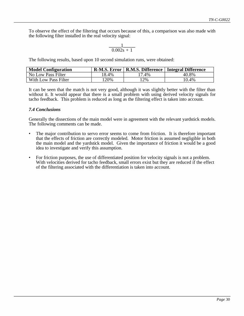
To observe the effect of the filtering that occurs because of this, a comparison was also made with the following filter installed in the real velocity signal:

_____1_____ 0.002s + 1

The following results, based upon 10 second simulation runs, were obtained: Model Configuration R-M.S. Error R.M.S. Difference Integral Difference No Low Pass Filter 18.4% 17.4% 40.8% With Low Pass Filter 120% 12% 10.4% It can be seen that the match is not very good, although it was slightly better with the filter than without it. It would appear that there is a small problem with using derived velocity signals for tacho feedback. This problem is reduced as long as the filtering effect is taken into account. 7.4 Conclusions Generally the dissections of the main model were in agreement with the relevant yardstick models. The following comments can be made. • The major contribution to servo error seems to come from friction. It is therefore important

that the effects of friction are correctly modeled. Motor friction is assumed negligible in both the main model and the yardstick model. Given the importance of friction it would be a good idea to investigate and verify this assumption.

• For friction purposes, the use of differentiated position for velocity signals is not a problem.

With velocities derived for tacho feedback, small errors exist but they are reduced if the effect of the filtering associated with the differentiation is taken into account.

TN-C-G0022

Page 31

8.0 Baseline Cases: Description and Justification The cases described here are meant as a coarse envelope over which to evaluate image smear performance. There are three different servoed axes which accept positional commands: altitude, azimuth, and cassegrain. The axes are excited individually with commands that are denoted either slow, typical or fast. It is assumed that the different axes do not couple together so that the effects may be RSS-ed (root sum squared) to produce a net RMS image smear. Runs are made with the tip-tilt secondary both active and inactive, in order to gain an understanding of the relative effect of tip-tilt upon the different error sources. The different error sources considered are friction, angle encoder A/D quantization, motor commanded rate D/A quantization, tip-tilt measurement noise, motor torque noise, drive eccentricity, and tachometer errors. Each error source acting alone is examined, as well as the combination of all error sources simultaneously. 8.1 Slow tracking cases The slow cases in the first section of table 2 are meant to demonstrate the effect of stick-slip at some disadvantageous points on the sky. For altitude, the near-zenith case shows a slowing down and then a reversal of velocity. For azimuth and cassegrain, the slow case is near the horizon. Position is modeled as a parabola, which makes the velocity pass through zero. The starting velocity and acceleration are taken from a program written by Rick McGonegal. 8.2 Typical tracking cases The so-called "typical" cases in the middle section of table 2 are meant to approximate a sidereal tracking rate of 15 arcseconds/second (7.3e-5 rad/sec). Rates 10 times faster and 10 times slower are also examined as part of the typical runs. 8.3 Fast Tracking Cases The fast cases in the bottom third of table 2 are for azimuth and cassegrain 0.5 degrees (8.7e-3 rad) from zenith, where tracking rates approach 0.5 deg/sec (8.7e-3 rad/sec).

TN-C-G0022

Page 32

9.0 Results of Baseline Model Runs Tables 3 through 6 show some of the results of the simulation for tip-tilt turned on. The results are quoted in the net RMS image smear in radians for both axes of the image plane combined. The four tables differ according to commanded motion of the telescope: altitude sidereal rate command, an azimuth sidereal rate command, a cassegrain sidereal rate command, and a near-zenith case. The near zenith case has the azimuth and cassegrain moving very quickly (0.5 deg/sec=0.009 rad/sec) and in opposite directions. The first line of data in Table 3 corresponds to the altitude command with the error sources turned off, and is labeled the benign case. This is not meant to be representative of a physically realistic case, but rather is used to demonstrate how much image smear the simulation would report in the absence of the modeled errors. Most of the error for the benign case is expected to be due to the transient response of the control loop. The modeled error sources are bearing friction, position encoder quantization, motor D/A converter quantization, tachometer ripple, motor torque noise, drive eccentricity, and tip-tilt measurement noise. The second line in Table 3 is labeled the "baseline" case and is thought to represent what is realistically obtainable since it contains the seven error sources described above. The RMS image smear, in radians of centroid motion, is 4.32e-8 radians after tip-tilt compensation. This represents about 0.012 arcseconds increase in the 50% encircled energy diameter. Among the error sources modeled, tip-tilt measurement noise is the largest contributor to image smear followed by friction. The random time-varying component of friction is responsible for nearly all of the friction induced error. It might be worth examining both the magnitude and bandwidth (time constant) of the model for time-varying bearing friction. The encoder quantization is varied by several orders of magnitude in Table 3. Predictably, the very large encoder errors cause large image smear. For small errors, near the baseline case, the encoder is a minor contributor to image smear, so the RMS does not change significantly. Changing the commanded altitude rate over several orders of magnitude did not show a large change in RMS error. The motor voltage D/A converter quantization was examined at 0.1 and 10 times the nominal values. As expected, the larger quantization errors produced more image smear. The sensitivity of image smear to motor D/A quantization is closely related to the analog motor loop. Since this is the second greatest contributor to image smear, it would be advisable to examine how the inner loop is made on the real telescope, paying specific attention to the voltage compensation. The last seven lines of Table 3 show the effect of each error source by itself. The tip-tilt measurement noise is found to be the third largest for altitude, causing an RMS error of 3.44e-8 with no other errors present. The RMS values for the noise sources alone do not root-sum-square to equal the RMS of the baseline case because the simulation is nonlinear and the error sources have a reinforcing effect that is slightly greater than the RSS.

TN-C-G0022

Page 33

The baseline case for azimuth command in Table 4 shows an RMS of 4.11e-8 rad. The cassegrain baseline case of Table 5 has image smear near that of altitude: 7.76e-8 rad. The fast tracking, near zenith condition of Table 6 has an RMS of 7.75e-8 rad, which is virtually the same as the typical speed case. It is thought that the reason why the fast case is so close to the typical case is that the random component of friction is dominant and is not changed between the two cases. Tables 7 through 10 correspond to Tables 3 through 6, described above, except that tip-tilt compensation has been turned off. Of course the errors are larger than for the earlier tables. The last table, Table 10, has a larger than expected error for the benign case. It is expected that this is due to a cross-coupling effect. For example, a rotation in the azimuth axis (i.e. z-azis) of the tube might be producing some motion in the x-axis. Since the azimuth velocity is high for the near-zenith case, the error ramps up to an appreciable amount of image smear, in this case about 1e-8 rad. 9.0.1 Stick Slip Results Figures 9.0.1 through 9.0.6 show the effect of very slow tracking, and correspond to cases numbered 1 through 6 in table 2. The first 3 of these figures are for tip-tilt and its associated noise turned off, while the last 3 figures are for tip-tilt active. Figure 9.0.1 is for the altitude axis near zenith with tip-tilt control turned off. The midpoint of this 100 second run corresponds to zero velocity. The upper left plot of figure 9.0.1 shows the commanded and achieved altitude position. The altitude axis moves in increments of between 6e-8 and 2e-7. These movements are two to six times larger than the encoder quantization step size of 3.3e-8 rad. For each small step the altitude motors abruptly jump to the new position, as evidenced by the periodic activity in the commanded voltage in the upper right. The tracking error over time is shown in the lower left of figure 9.0.1. The filtered RMS image smear in the lower right of figure 9.0.1 might seem surprisingly small. It should be noted that the RMS was taken first, then this was filtered with 1 second time constant. Had it been filtered then RMS applied, it would have erroneously reduced the RMS. The filtering process described is one which effectively gives a moving average of the RMS error. The fact that the image smear is smaller than the baseline case is due to the removal of the two largest error sources: tip-tilt measurement noise and random friction. The tip-tilt measurement noise is absent because tip-tilt is inactive, and the random friction component is masked because it is not great enough to overcome the static friction. Figure 9.0.2 shows the azimuth axis under slow tracking with the tip-tilt secondary control inactive. The command is much larger for the azimuth axis than for the altitude axis shown in the previous plot, tending to obscure the discrete steps in the azimuth axis. The azimuth axis command is larger because the azimuth axis moves very quickly near the zenith. From the tracking error, it appears that the error steps are around 3e-8 radians, approximately equal to the azimuth encoder step size of 2.4e-8. So for azimuth it seems that the stick-slip would occur in

TN-C-G0022

Page 34

steps smaller than the presently modeled encoder size. This could be tested by forcing the simulation to have an artificially small azimuth encoder step size. The Gemini results compare approximately to the simulation results for the VLT as reported in reference [4]. In that report, the tracking error has an RMS of 0.11 arcseconds before compensation and 0.006 arcseconds after tip-tilt compensation. The Gemini tracking error is around 0.008 arcseconds RMS before compensation, about ten times smaller than the VLT. It is not known why the Gemini model diverges so strongly from the VLT model. This could be an indication that the Gemini model has an overly optimistic model of the nonlinear bearing friction. The Gemini results after tip-tilt compensation are still about 0.008 arcseconds, being dominated by the tip-tilt measurement noise which seems to have been neglected in the VLT report. Both the VLT and Gemini results are for tracking rates of approximately 0.1 arcsec/sec. Figure 9.0.3 shows that the cassegrain control loop is dominated by the encoder step size of 4.9e-6 radians. Figure 9.0.4 shows the altitude response again under slow tracking, but this time with tip-tilt activated. The image smear with tip-tilt active, figure 9.0.4, appears slightly smaller than for the same case with tip-tilt inactive, figure 9.0.1, because of the large tip-tilt measurement noise introduced by the CCD centroiding error. Figure 9.0.5 shows that tip-tilt also degrades the azimuth slow tracking, again due to the tip-tilt measurement noise. Figure 9.0.6 for the cassegrain slow tracking error is smaller than the angular encoder quantization, and the tip-tilt measurement noise is again the largest contributor to image smear. 9.1 Comparative Effect of Tip-Tilt upon Various Image Smear Error Sources For the altitude axis, the overall effect of tip-tilt if to reduce the image smear from 1.09e-7 to 4.32e-8 radians. This is a modest savings of factor 2.5 in RMS or 6.4 in power. The biggest reason why the improvement is so small is that the tip-tilt measurement noise (CCD centroiding error) is broadband and virtually unaffected by the tip-tilt control. For all of the runs in this report, windshake induced disturbance was absent. Perhaps it is better to view tip-tilt as a sunk cost. That is, the cost of using tip-tilt (i.e. measurement noise) has already been paid since it will be required to attenuate windshake disturbances and atmospheric errors. Ignoring the tip-tilt measurement noise, the improvement provided by tip-tilt for altitude errors is a reduction from 1.09e-7 rad to 2.56e-8 rad, giving a factor of 4.3 in RMS or 18.1 in power. Tip-tilt control of the secondary will provide different levels of improvement to the different error sources because of their different frequency content. For example, the altitude friction induced error is reduced by a factor of 6.7 in RMS. Altitude encoder quantization has an improvement of 3.4. Motor D/A conversion errors are relatively unaffected by tip-tilt. Motor torque variation disturbances are improved by a factor of 1.8 in RMS. The very slowly changing drive eccentricity and tachometer induced errors enjoy RMS improvements of 57 and 107 respectively. These latter

TN-C-G0022

Page 35

levels of improvement are likely to be unrealistic. The higher harmonics, though smaller in disturbance magnitude, will get less attenuation and probably be much more significant to the image smear. The effect of tip-tilt upon azimuth errors is similar to the effect for altitude errors described above, but the effect upon cassegrain errors is significantly different. As described in section 5.3 above, tip-tilt tends to increase image smear errors from the cassegrain control loop rather than attenuating the errors. The increases quoted here are for a pessimistic relative placement of the guide object and science object (i.e. 180 degrees opposed, and each at the edge of its respective field). It is generally preferred in control systems to have high frequency measurement noise and low frequency disturbances. Since the errors in cassegrain tracking are analogous to measurement errors, it is expected that the higher frequency errors will be only slightly increased, while low frequency errors will be successfully tracked. Successful tip-tilt tracking of errors on the guide object causes pathological addition of errors to the science object. The errors due to friction are increased by a factor of 2.3 in RMS. Cassegrain encoder quantization errors and motor D/A conversion errors increase by a factor of 1.2 under tip-tilt. The motor torque variation errors are unexpectedly improved by a factor of 1.6. The drive eccentricity and tachometer errors are increased by factors of 1.4 and 3.0 respectively. 9.2 Sensitivity of Image Smear to Various Error Sources It is often assumed that the effects of error sources can be RSS-ed (root sum squared) to arrive at a net error. This assumes that the error sources are decorrelated and that the simulation is linear. Since the telescope servo simulation has a number of nonlinearities, this section shows the results of some cross-correlation testing. For each case described in table 12, the image smear was calculated over a surface defined by varying two possibly related parameters. The x and y axes contain normalized values of the parameters, with an X representing the nominal value. The z-axis represents the RMS image smear centroid in radians. Since each parameter is varied over 20 different values in each plot, the 20x20 grid of 400 runs takes slightly less than 2 days to run using Matlab 4.0 on a Pentium-60 PC. Many of the plots shown in figures 9.2.1 through 9.2.18 show some interesting effects. Figure 9.2.1 for example shows that there is some region where increasing altitude rate actually decreases the RMS image smear, perhaps due to the presence or absence of particular structural modes being excited. Figure 9.2.2 shows that the relative amount of friction has a much stronger effect on image smear than the commanded rate for the azimuth axis. At about 4 times the modeled amount of friction, i.e. at 5000 Nm, a step is reached where the simulation breaks down and performance degrades badly. Figure 9.2.3 shows that when the A/D converter on azimuth commanded rate is about 3 times coarser than the nominal amount, the control system becomes more sensitive to changes in friction.

TN-C-G0022

Page 36

Figure 9.2.4 shows that the altitude axis becomes more sensitive to friction if the A/D converter on altitude commanded rate is about 4 times coarser than nominal. The normal level is nominally shown as 5, so the 4 times level is shown as 20 in the graph. Figure 9.2.5 shows that both tracking rate and the stiction/coulomb friction ratio are well behaved for the altitude axis. The image smear increases in a very smooth, linear manner with either parameter. Figure 9.2.6 shows that the cassegrain axis is nonlinear in its response to both motor torque noise and angular quantization stepsize. There are many peaks and valleys in the plot, unlike the monotonically increasing plot which one would find with a linear system subject to linear error sources. Figure 9.2.7 shows that the altitude axis is relatively insensitive to changes in the ratio of friction/coulomb friction and to the D/A converter motor quantization stepsize. Figure 9.2.8 shows that the altitude axis is relatively insensitive to changes in the motor torque noise and D/A converter motor quantization stepsize. Figure 9.2.9 shows that the azimuth axis becomes more sensitive to torqnoise errors when the D/A converter motor quantization stepsize is made 2 to 3 times coarser than the nominal value. Figure 9.2.10 shows that the altitude axis is considerably more sensitive to changes in the amount of friction than it is to changes in the motor torque noise. Figure 9.2.11 shows that the azimuth axis has some nonlinear sensitivity to the amount of friction and motor torque noise, since the graph is not monotonically increasing for either axis. Figure 9.2.12 shows that the cassegrain axis has considerable nonlinear interaction between the amount of friction and the motor torque noise variations. Figure 9.2.13 shows that when the ratio of stiction to coulomb friction on the azimuth axis is increased 2 to 3 times its nominal value, the azimuth response to torque errors becomes much more nonlinear. Figure 9.2.14 shows that, for the altitude axis, the motor torque noise interacts in a significantly nonlinear way with the ratio of stiction to coulomb friction. Figure 9.2.15 shows that when the ratio of stiction to coulomb friction is increased from the nominal value, the cassegrain axis becomes more nonlinear with respect to motor torque noise. Figure 9.2.16 shows that the image smear for the altitude axis increases very sharply as the time constant drops for the random component of bearing friction. This is because the frictional disturbances become larger bandwidth, and the altitude controller loses the ability to counteract the large variation in frictional torque.

TN-C-G0022

Page 37

Figure 9.2.17 shows that the azimuth axis is also sensitive to reduction in the frictional time constant, especially if the magnitude of friction is increased. Figure 9.2.18 shows that the cassegrain performance becomes quite poor if either the magnitude of friction is increased or the time constant is decreased, as expected. Figure 9.2.19 shows that the cassegrain axis is more sensitive to the magnitude of friction than to the tracking rate, but that the two effects combine in a fairly smooth, linear manner. Figure 9.2.20 shows that the magnitude of friction and tracking rate for the altitude axis combine in a rather linear way.

TN-C-G0022

Page 38

10.0 Conclusions This report describes the simulation of the telescope structure and control system. Servo system related error sources are included, and the effect of the tip-tilt secondary mirror is quantified. Errors associated with the cassegrain rotator seem large and are rather uncertain, potentially leading to a significant performance risk.

TN-C-G0022

Page 39

11.0 Future Work • Tune the controllers to give the best image smear error subject to the best estimated levels of

error sources. This is equivalent to choosing the best bandwidth to minimize the sum of measurement noise (for which low bandwidth is preferred) and disturbance rejection (for which high bandwidth is preferred).

• Verify the level of angular measurement noise on the tip-tilt signal, since this error is the

largest contributor to image smear. • Examine the model of bearing friction paying particular attention to the stochastic component

of friction. This part of bearing friction is noticed to be the second largest contributor to image smear. There seems to be considerable risk in using the image smear errors produced because the random component of friction could be much larger or smaller than the values modeled. The character of the stick-slip region is also strongly dependent upon nonlinear friction model.

• Get more realistic estimates of error sources for the cassegrain rotator drive motors and drive

train. Many of the parameters, such as systematic motor torque ripple and drive eccentricity, are currently modeled coarsely based on analogy to the altitude and azimuth axes. It would also be desirable to model the disturbance torques due to the effect of the cable-rap, both in magnitude and frequency content. The errors in the cassegrain axis appear to contribute more to image smear than errors in altitude and azimuth combined, for the nominal amounts assumed in the simulation. Since the cassegrain error sources are poorly known, this appears to be a large performance risk.

• The slewing controller should be extended to the cassegrain axis. This would enforce the

velocity and acceleration constraints. • Resolve the problem of why the near-zenith cassegrain errors show a large ramp (1e-8 rad) in

image smear even when error sources are removed. This is expected to be a cross-coupling present in the finite-element analysis of the mount or tube structures.

• What are the magnitudes of higher harmonics of motor torque variation and tachometer

errors?

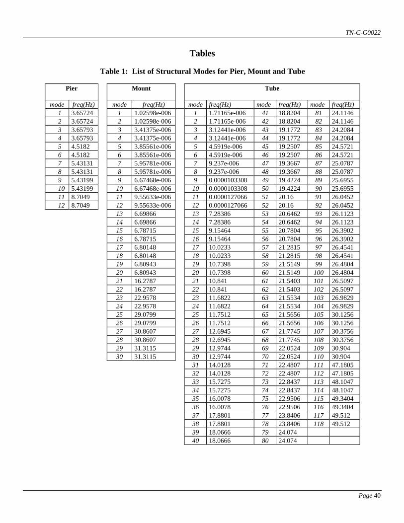
TN-C-G0022

Page 40

Tables

Table 1: List of Structural Modes for Pier, Mount and Tube

Pier

Mount

Tube

mode freq(Hz) mode freq(Hz) mode freq(Hz) mode freq(Hz) mode freq(Hz) 1 3.65724 1 1.02598e-006 1 1.71165e-006 41 18.8204 81 24.1146 2 3.65724 2 1.02598e-006 2 1.71165e-006 42 18.8204 82 24.1146 3 3.65793 3 3.41375e-006 3 3.12441e-006 43 19.1772 83 24.2084 4 3.65793 4 3.41375e-006 4 3.12441e-006 44 19.1772 84 24.2084 5 4.5182 5 3.85561e-006 5 4.5919e-006 45 19.2507 85 24.5721 6 4.5182 6 3.85561e-006 6 4.5919e-006 46 19.2507 86 24.5721 7 5.43131 7 5.95781e-006 7 9.237e-006 47 19.3667 87 25.0787 8 5.43131 8 5.95781e-006 8 9.237e-006 48 19.3667 88 25.0787 9 5.43199 9 6.67468e-006 9 0.0000103308 49 19.4224 89 25.6955 10 5.43199 10 6.67468e-006 10 0.0000103308 50 19.4224 90 25.6955 11 8.7049 11 9.55633e-006 11 0.0000127066 51 20.16 91 26.0452 12 8.7049 12 9.55633e-006 12 0.0000127066 52 20.16 92 26.0452 13 6.69866 13 7.28386 53 20.6462 93 26.1123 14 6.69866 14 7.28386 54 20.6462 94 26.1123 15 6.78715 15 9.15464 55 20.7804 95 26.3902 16 6.78715 16 9.15464 56 20.7804 96 26.3902 17 6.80148 17 10.0233 57 21.2815 97 26.4541 18 6.80148 18 10.0233 58 21.2815 98 26.4541 19 6.80943 19 10.7398 59 21.5149 99 26.4804 20 6.80943 20 10.7398 60 21.5149 100 26.4804 21 16.2787 21 10.841 61 21.5403 101 26.5097 22 16.2787 22 10.841 62 21.5403 102 26.5097 23 22.9578 23 11.6822 63 21.5534 103 26.9829 24 22.9578 24 11.6822 64 21.5534 104 26.9829 25 29.0799 25 11.7512 65 21.5656 105 30.1256 26 29.0799 26 11.7512 66 21.5656 106 30.1256 27 30.8607 27 12.6945 67 21.7745 107 30.3756 28 30.8607 28 12.6945 68 21.7745 108 30.3756 29 31.3115 29 12.9744 69 22.0524 109 30.904 30 31.3115 30 12.9744 70 22.0524 110 30.904 31 14.0128 71 22.4807 111 47.1805 32 14.0128 72 22.4807 112 47.1805 33 15.7275 73 22.8437 113 48.1047 34 15.7275 74 22.8437 114 48.1047 35 16.0078 75 22.9506 115 49.3404 36 16.0078 76 22.9506 116 49.3404 37 17.8801 77 23.8406 117 49.512 38 17.8801 78 23.8406 118 49.512 39 18.0666 79 24.074 40 18.0666 80 24.074

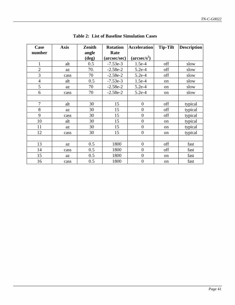
TN-C-G0022

Page 41

Table 2: List of Baseline Simulation Cases

Case

number Axis Zenith

angle (deg)

Rotation Rate

(arcsec/sec)

Acceleration

(arcsec/s2)

Tip-Tilt Description

1 alt 0.5 -7.53e-3 1.5e-4 off slow 2 az 70. -2.58e-2 5.2e-4 off slow 3 cass 70 -2.58e-2 5.2e-4 off slow 4 alt 0.5 -7.53e-3 1.5e-4 on slow 5 az 70 -2.58e-2 5.2e-4 on slow 6 cass 70 -2.58e-2 5.2e-4 on slow 7 alt 30 15 0 off typical 8 az 30 15 0 off typical 9 cass 30 15 0 off typical

10 alt 30 15 0 on typical 11 az 30 15 0 on typical 12 cass 30 15 0 on typical

13 az 0.5 1800 0 off fast 14 cass 0.5 1800 0 off fast 15 az 0.5 1800 0 on fast 16 cass 0.5 1800 0 on fast

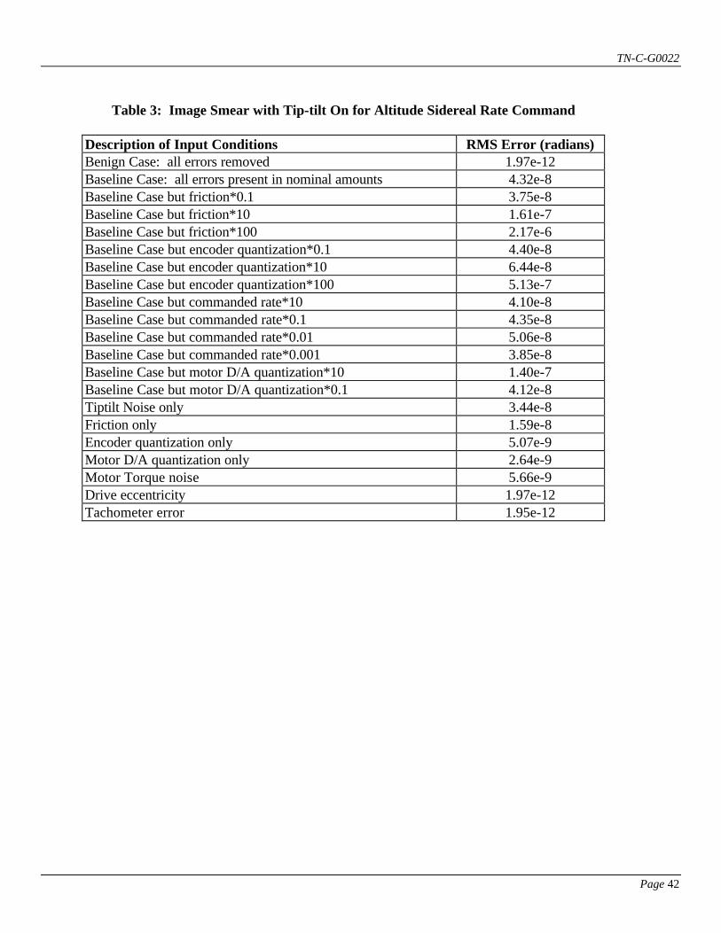
TN-C-G0022

Page 42

Table 3: Image Smear with Tip-tilt On for Altitude Sidereal Rate Command

Description of Input Conditions RMS Error (radians) Benign Case: all errors removed 1.97e-12 Baseline Case: all errors present in nominal amounts 4.32e-8 Baseline Case but friction*0.1 3.75e-8 Baseline Case but friction*10 1.61e-7 Baseline Case but friction*100 2.17e-6 Baseline Case but encoder quantization*0.1 4.40e-8 Baseline Case but encoder quantization*10 6.44e-8 Baseline Case but encoder quantization*100 5.13e-7 Baseline Case but commanded rate*10 4.10e-8 Baseline Case but commanded rate*0.1 4.35e-8 Baseline Case but commanded rate*0.01 5.06e-8 Baseline Case but commanded rate*0.001 3.85e-8 Baseline Case but motor D/A quantization*10 1.40e-7 Baseline Case but motor D/A quantization*0.1 4.12e-8 Tiptilt Noise only 3.44e-8 Friction only 1.59e-8 Encoder quantization only 5.07e-9 Motor D/A quantization only 2.64e-9 Motor Torque noise 5.66e-9 Drive eccentricity 1.97e-12 Tachometer error 1.95e-12

TN-C-G0022

Page 43

Table 4: Image Smear with Tip-tilt On for Azimuth Sidereal Rate Command

Description of Input Conditions RMS Error (radians) Benign Case: all errors removed 2.09e-12 Baseline Case: all errors present in nominal amounts 4.11e-8 Baseline Case but friction*0.1 4.02e-8 Baseline Case but friction*10 9.94e-8 Baseline Case but friction*100 4.24e-6 Baseline Case but encoder quantization*0.1 3.77e-8 Baseline Case but encoder quantization*10 4.92e-8 Baseline Case but encoder quantization*100 3.18e-7 Baseline Case but commanded rate*10 3.98e-8 Baseline Case but commanded rate*0.1 3.99e-8 Baseline Case but commanded rate*0.01 4.32e-8 Baseline Case but commanded rate*0.001 3.87e-8 Baseline Case but motor D/A quantization*10 7.61e-8 Baseline Case but motor D/A quantization*0.1 3.78e-8 Tiptilt Noise only 3.44e-8 Friction only 5.79e-9 Encoder quantization only 3.04e-9 Motor D/A quantization only 5.31e-9 Motor torque noise 5.64e-9 Drive eccentricity 2.07e-12 Tachometer error 2.29e-12

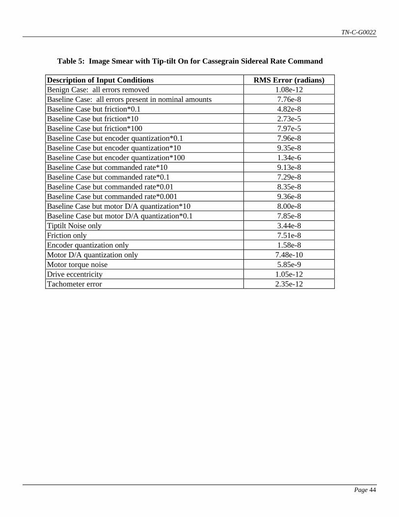
TN-C-G0022

Page 44

Table 5: Image Smear with Tip-tilt On for Cassegrain Sidereal Rate Command

Description of Input Conditions RMS Error (radians) Benign Case: all errors removed 1.08e-12 Baseline Case: all errors present in nominal amounts 7.76e-8 Baseline Case but friction*0.1 4.82e-8 Baseline Case but friction*10 2.73e-5 Baseline Case but friction*100 7.97e-5 Baseline Case but encoder quantization*0.1 7.96e-8 Baseline Case but encoder quantization*10 9.35e-8 Baseline Case but encoder quantization*100 1.34e-6 Baseline Case but commanded rate*10 9.13e-8 Baseline Case but commanded rate*0.1 7.29e-8 Baseline Case but commanded rate*0.01 8.35e-8 Baseline Case but commanded rate*0.001 9.36e-8 Baseline Case but motor D/A quantization*10 8.00e-8 Baseline Case but motor D/A quantization*0.1 7.85e-8 Tiptilt Noise only 3.44e-8 Friction only 7.51e-8 Encoder quantization only 1.58e-8 Motor D/A quantization only 7.48e-10 Motor torque noise 5.85e-9 Drive eccentricity 1.05e-12 Tachometer error 2.35e-12

TN-C-G0022

Page 45

Table 6: Image Smear with Tip-tilt On for Azimuth and Cassegrain Near-zenith

Rate Command of 0.5 deg/sec.

Description of Input Conditions RMS Error (radians) Benign Case: all errors removed 3.00e-10 Baseline Case: all errors present in nominal amounts 7.75e-8 Baseline Case but friction*0.1 3.62e-8 Baseline Case but friction*10 2.64e-4 Baseline Case but friction*100 3.97e-4 Baseline Case but encoder quantization*0.1 7.88e-8 Baseline Case but encoder quantization*10 1.13e-7 Baseline Case but encoder quantization*100 9.59e-7 Baseline Case but commanded rate*10 8.69e-6 Baseline Case but commanded rate*0.1 7.75e-8 Baseline Case but commanded rate*0.01 7.21e-8 Baseline Case but commanded rate*0.001 7.60-e8 Baseline Case but motor D/A quantization*10 7.75e-8 Baseline Case but motor D/A quantization*0.1 7.75e-8 Tiptilt Noise only 3.44e-8 Friction only 7.26e-8 Encoder quantization only 1.01e-8 Motor D/A quantization only 3.09e-10 Motor torque noise 3.90e-9 Drive eccentricity 3.22e-10 Tachometer error 2.01e-9

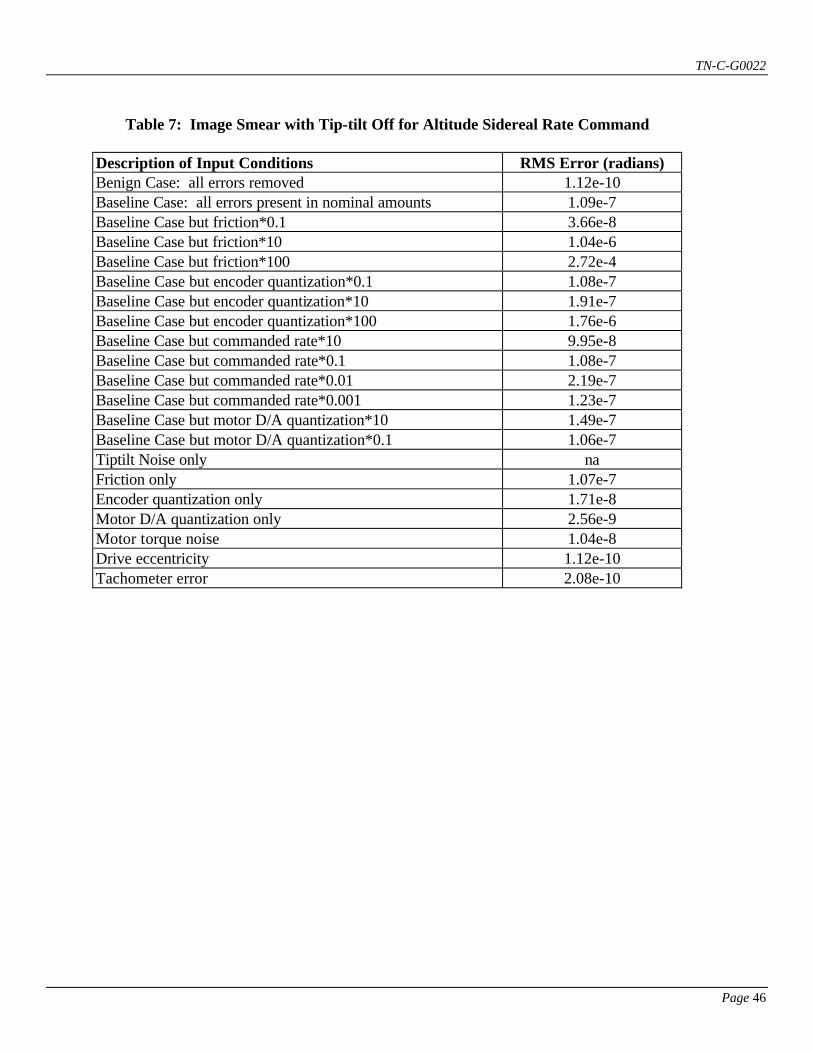
TN-C-G0022

Page 46

Table 7: Image Smear with Tip-tilt Off for Altitude Sidereal Rate Command

Description of Input Conditions RMS Error (radians) Benign Case: all errors removed 1.12e-10 Baseline Case: all errors present in nominal amounts 1.09e-7 Baseline Case but friction*0.1 3.66e-8 Baseline Case but friction*10 1.04e-6 Baseline Case but friction*100 2.72e-4 Baseline Case but encoder quantization*0.1 1.08e-7 Baseline Case but encoder quantization*10 1.91e-7 Baseline Case but encoder quantization*100 1.76e-6 Baseline Case but commanded rate*10 9.95e-8 Baseline Case but commanded rate*0.1 1.08e-7 Baseline Case but commanded rate*0.01 2.19e-7 Baseline Case but commanded rate*0.001 1.23e-7 Baseline Case but motor D/A quantization*10 1.49e-7 Baseline Case but motor D/A quantization*0.1 1.06e-7 Tiptilt Noise only na Friction only 1.07e-7 Encoder quantization only 1.71e-8 Motor D/A quantization only 2.56e-9 Motor torque noise 1.04e-8 Drive eccentricity 1.12e-10 Tachometer error 2.08e-10

TN-C-G0022

Page 47

Table 8: Image Smear with Tip-tilt Off for Azimuth Sidereal Rate Command


TN-C-G0022

Page 48

Table 9: Image Smear with Tip-tilt Off for Cassegrain Sidereal Rate Command


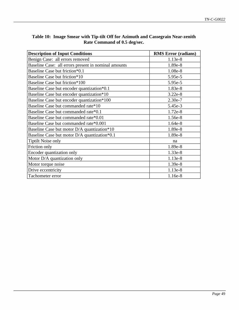
TN-C-G0022

Page 49

Table 10: Image Smear with Tip-tilt Off for Azimuth and Cassegrain Near-zenith

Rate Command of 0.5 deg/sec.


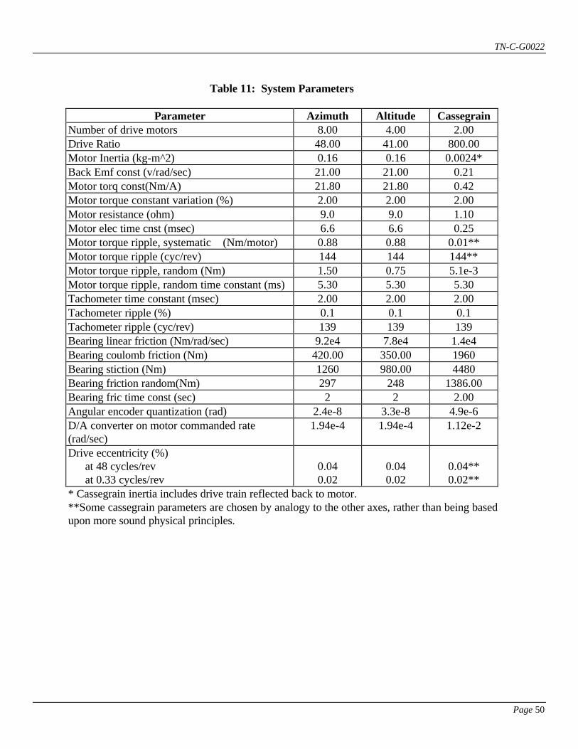
TN-C-G0022

Page 50

Table 11: System Parameters

Parameter Azimuth Altitude Cassegrain

Number of drive motors 8.00 4.00 2.00 Drive Ratio 48.00 41.00 800.00 Motor Inertia (kg-m^2) 0.16 0.16 0.0024* Back Emf const (v/rad/sec) 21.00 21.00 0.21 Motor torq const(Nm/A) 21.80 21.80 0.42 Motor torque constant variation (%) 2.00 2.00 2.00 Motor resistance (ohm) 9.0 9.0 1.10 Motor elec time cnst (msec) 6.6 6.6 0.25 Motor torque ripple, systematic (Nm/motor) 0.88 0.88 0.01** Motor torque ripple (cyc/rev) 144 144 144** Motor torque ripple, random (Nm) 1.50 0.75 5.1e-3 Motor torque ripple, random time constant (ms) 5.30 5.30 5.30 Tachometer time constant (msec) 2.00 2.00 2.00 Tachometer ripple (%) 0.1 0.1 0.1 Tachometer ripple (cyc/rev) 139 139 139 Bearing linear friction (Nm/rad/sec) 9.2e4 7.8e4 1.4e4 Bearing coulomb friction (Nm) 420.00 350.00 1960 Bearing stiction (Nm) 1260 980.00 4480 Bearing friction random(Nm) 297 248 1386.00 Bearing fric time const (sec) 2 2 2.00 Angular encoder quantization (rad) 2.4e-8 3.3e-8 4.9e-6 D/A converter on motor commanded rate (rad/sec)

1.94e-4 1.94e-4 1.12e-2

Drive eccentricity (%) at 48 cycles/rev at 0.33 cycles/rev

0.04 0.02

0.04 0.02

0.04** 0.02**

* Cassegrain inertia includes drive train reflected back to motor. **Some cassegrain parameters are chosen by analogy to the other axes, rather than being based upon more sound physical principles.

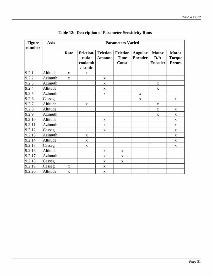
TN-C-G0022

Page 51

Table 12: Description of Parameter Sensitivity Runs

Figure

number Axis Parameters Varied

Rate Friction- ratio:

coulomb/ static

Friction Amount

Friction Time Const

Angular Encoder

Motor D/A

Encoder

Motor Torque Errors

9.2.1 Altitude x x 9.2.2 Azimuth x x 9.2.3 Azimuth x x 9.2.4 Altitude x x 9.2.5 Azimuth x x 9.2.6 Casseg x x 9.2.7 Altitude x x 9.2.8 Altitude x x 9.2.9 Azimuth x x 9.2.10 Altitude x x 9.2.11 Azimuth x x 9.2.12 Casseg x x 9.2.13 Azimuth x x 9.2.14 Altitude x x 9.2.15 Casseg x x 9.2.16 Altitude x x 9.2.17 Azimuth x x 9.2.18 Casseg x x 9.2.19 Casseg x x 9.2.20 Altitude x x

TN-C-G0022

Page 52

Figures

TN-C-G0022

Page 53

Figure 2.1: Top Level Simulation Block Diagram

TN-C-G0022

Page 54

Figure 4.1: Pier Structure

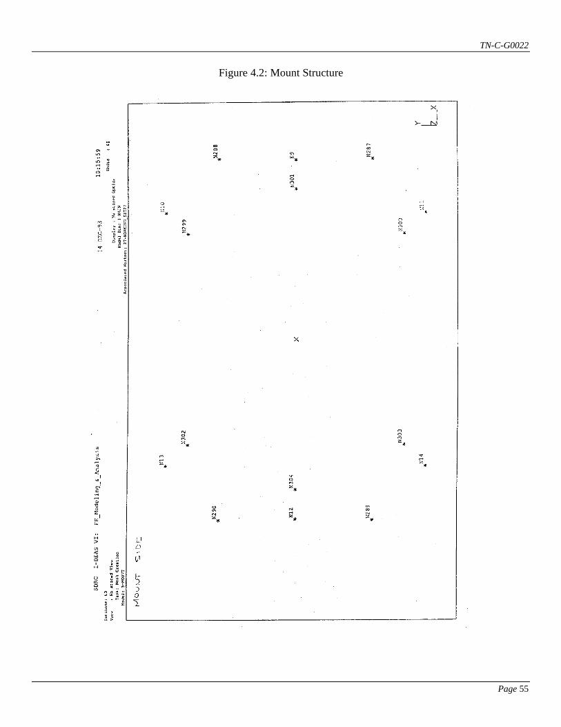
TN-C-G0022

Page 55

Figure 4.2: Mount Structure

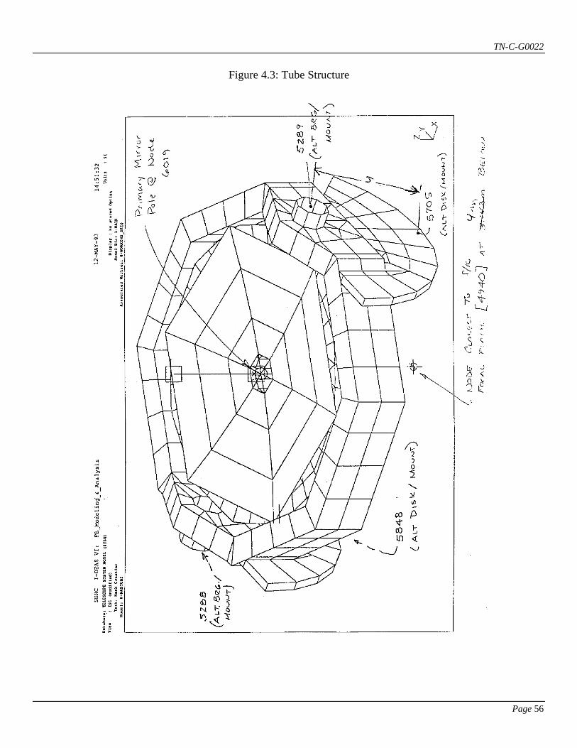
TN-C-G0022

Page 56

Figure 4.3: Tube Structure

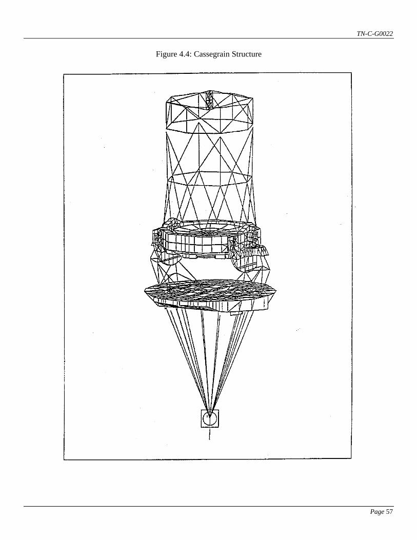
TN-C-G0022

Page 57

Figure 4.4: Cassegrain Structure

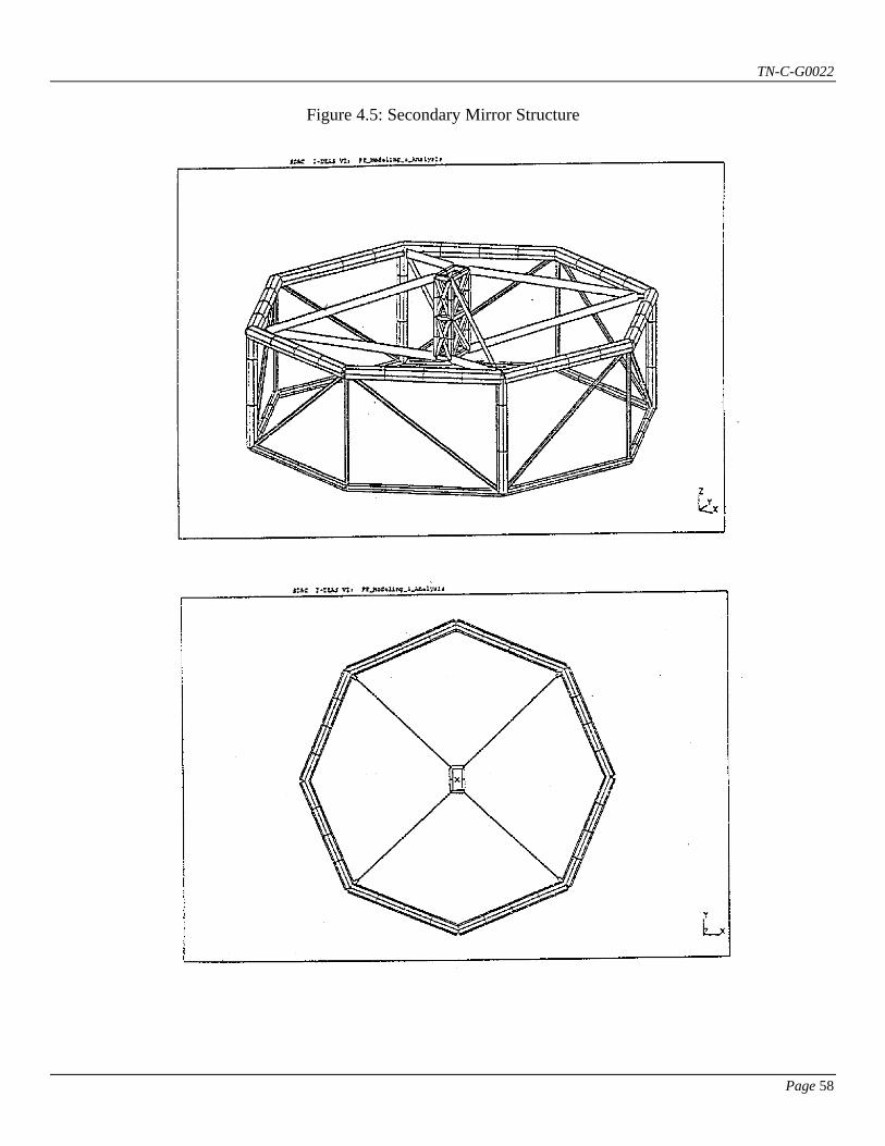
TN-C-G0022

Page 58

Figure 4.5: Secondary Mirror Structure

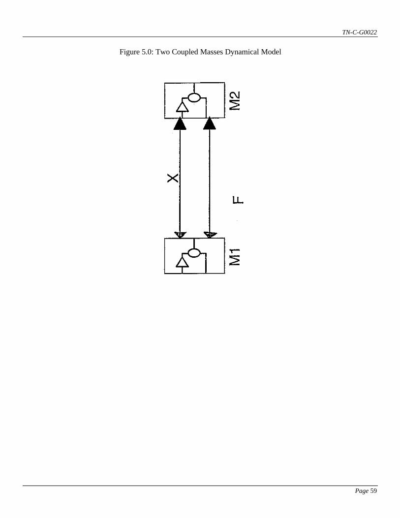
TN-C-G0022

Page 59

Figure 5.0: Two Coupled Masses Dynamical Model

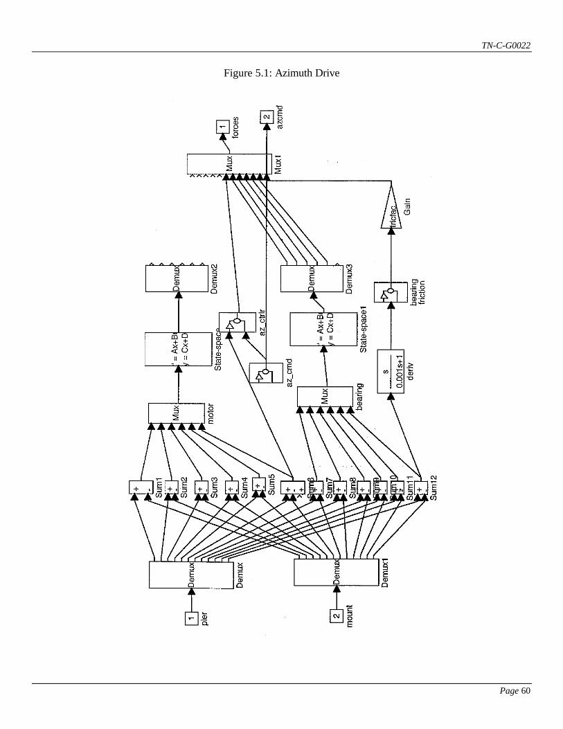
TN-C-G0022

Page 60

Figure 5.1: Azimuth Drive

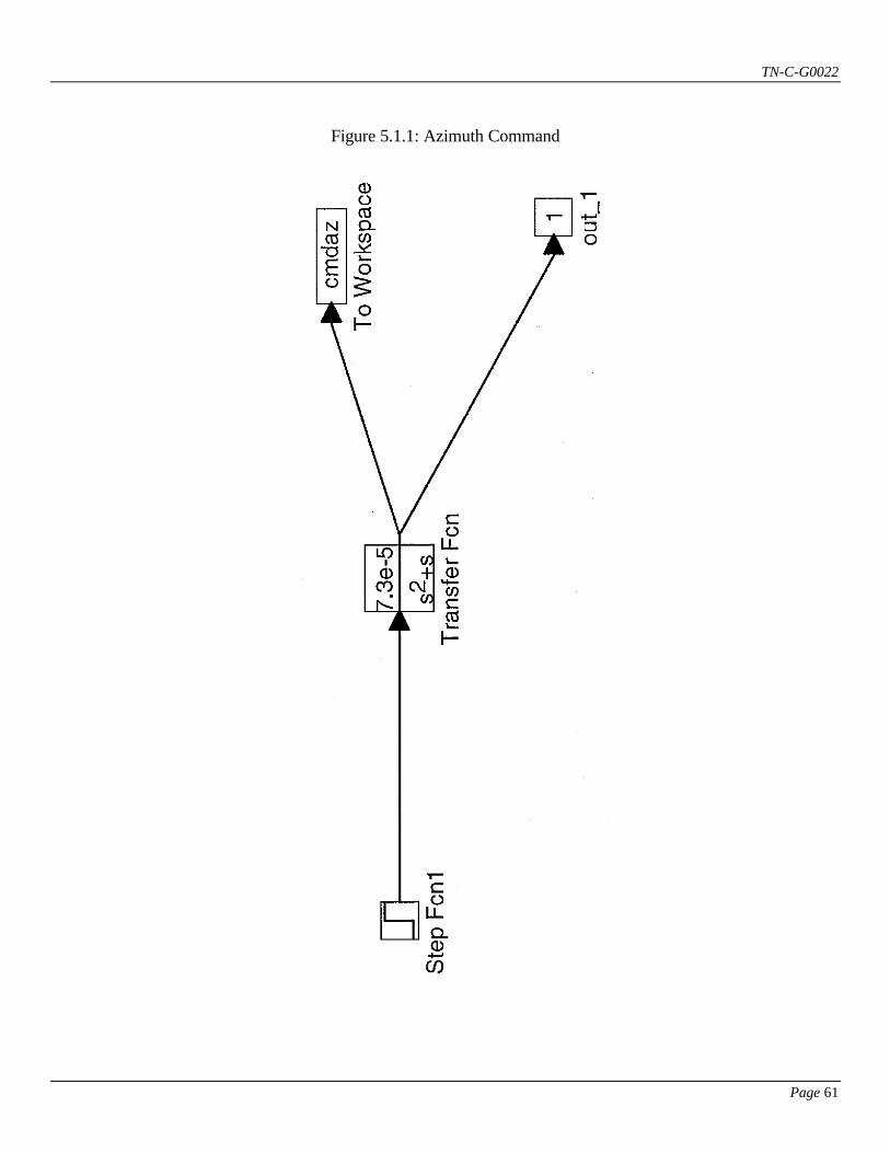
TN-C-G0022

Page 61

Figure 5.1.1: Azimuth Command

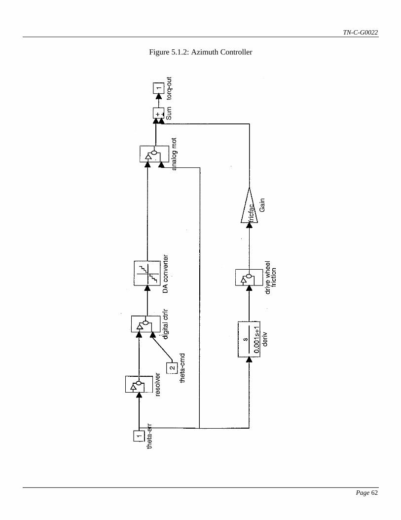
TN-C-G0022

Page 62

Figure 5.1.2: Azimuth Controller

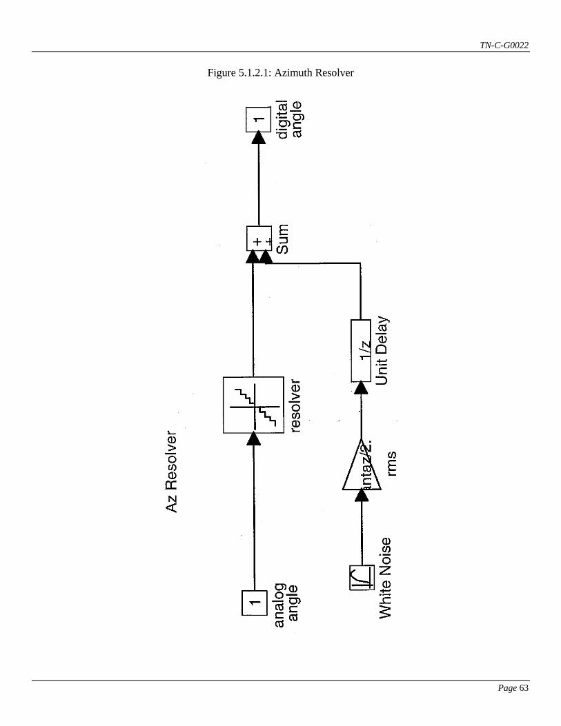
TN-C-G0022

Page 63

Figure 5.1.2.1: Azimuth Resolver

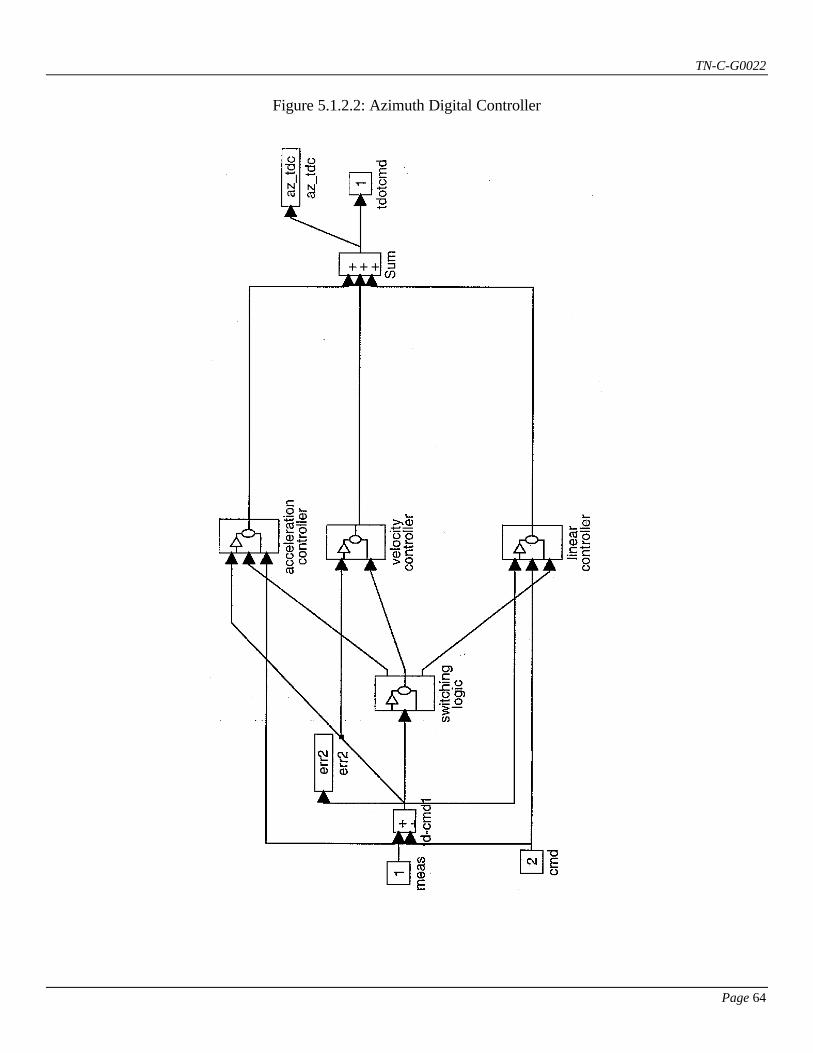
TN-C-G0022

Page 64

Figure 5.1.2.2: Azimuth Digital Controller

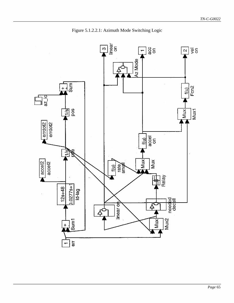
TN-C-G0022

Page 65

Figure 5.1.2.2.1: Azimuth Mode Switching Logic

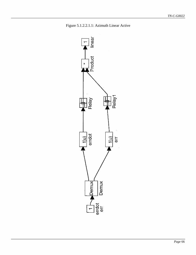
TN-C-G0022

Page 66

Figure 5.1.2.2.1.1: Azimuth Linear Active

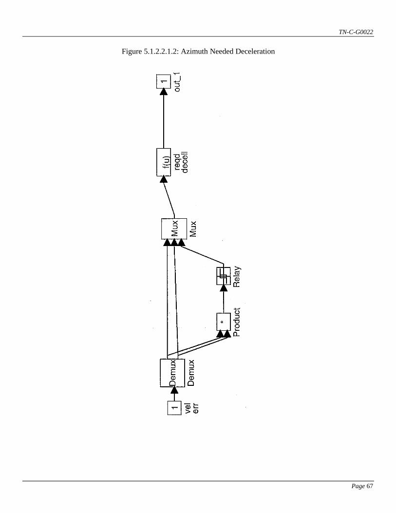
TN-C-G0022

Page 67

Figure 5.1.2.2.1.2: Azimuth Needed Deceleration

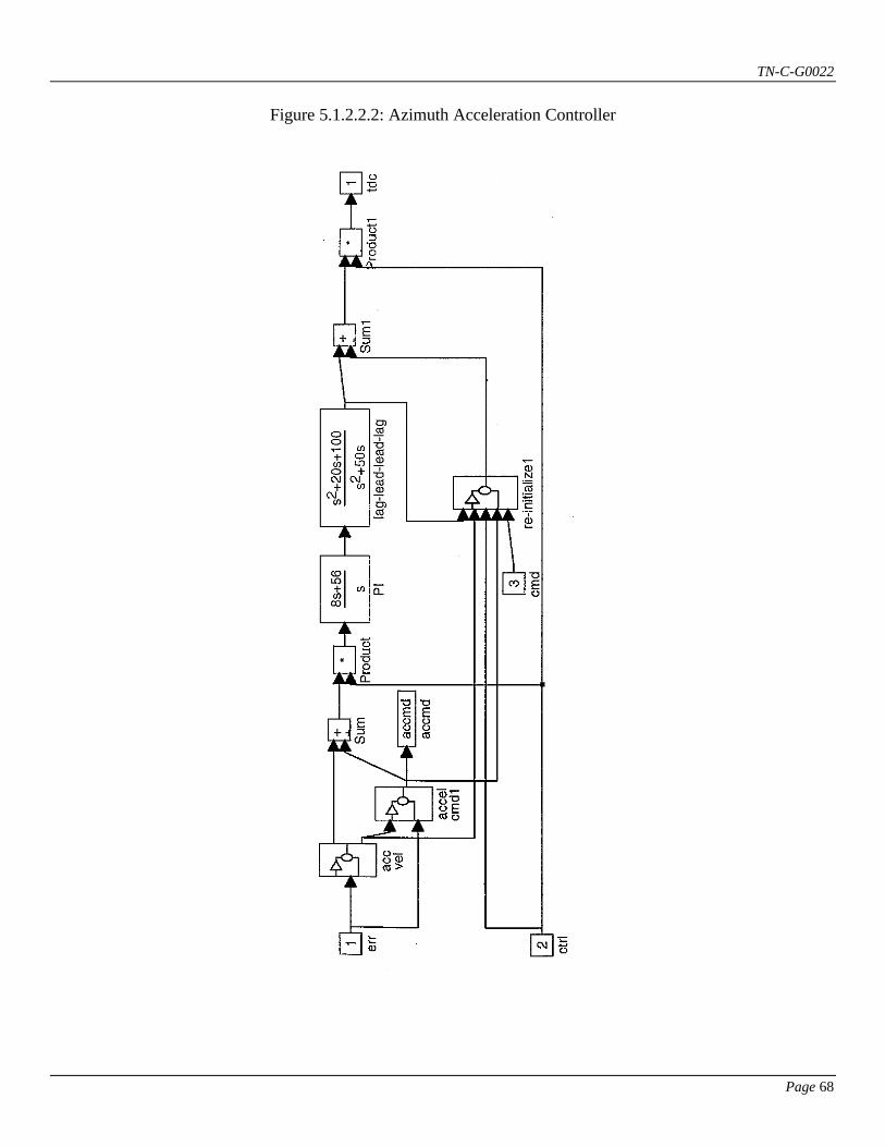
TN-C-G0022

Page 68

Figure 5.1.2.2.2: Azimuth Acceleration Controller

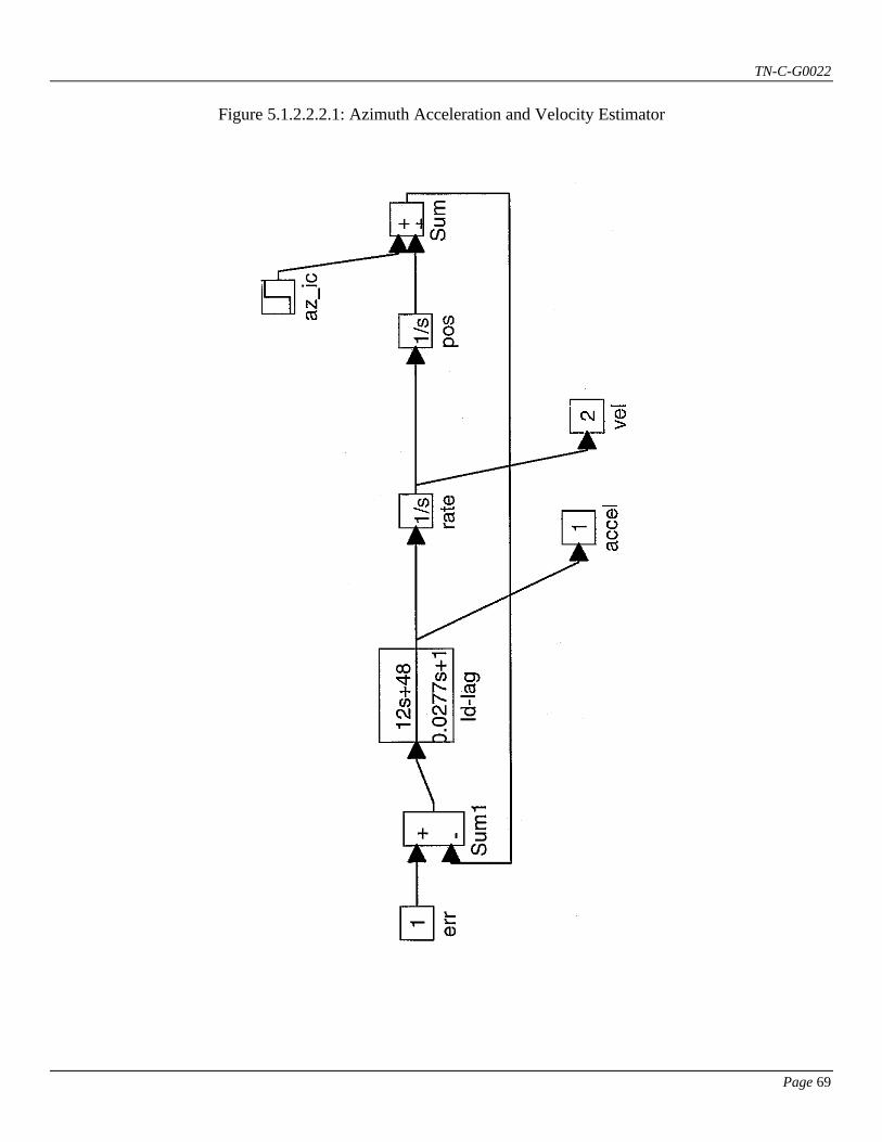
TN-C-G0022

Page 69

Figure 5.1.2.2.2.1: Azimuth Acceleration and Velocity Estimator

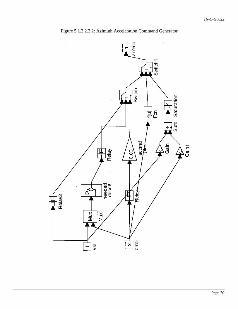
TN-C-G0022

Page 70

Figure 5.1.2.2.2.2: Azimuth Acceleration Command Generator

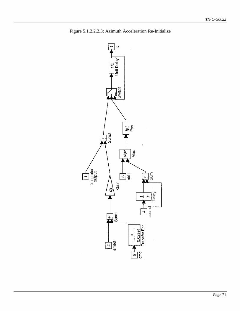
TN-C-G0022

Page 71

Figure 5.1.2.2.2.3: Azimuth Acceleration Re-Initialize

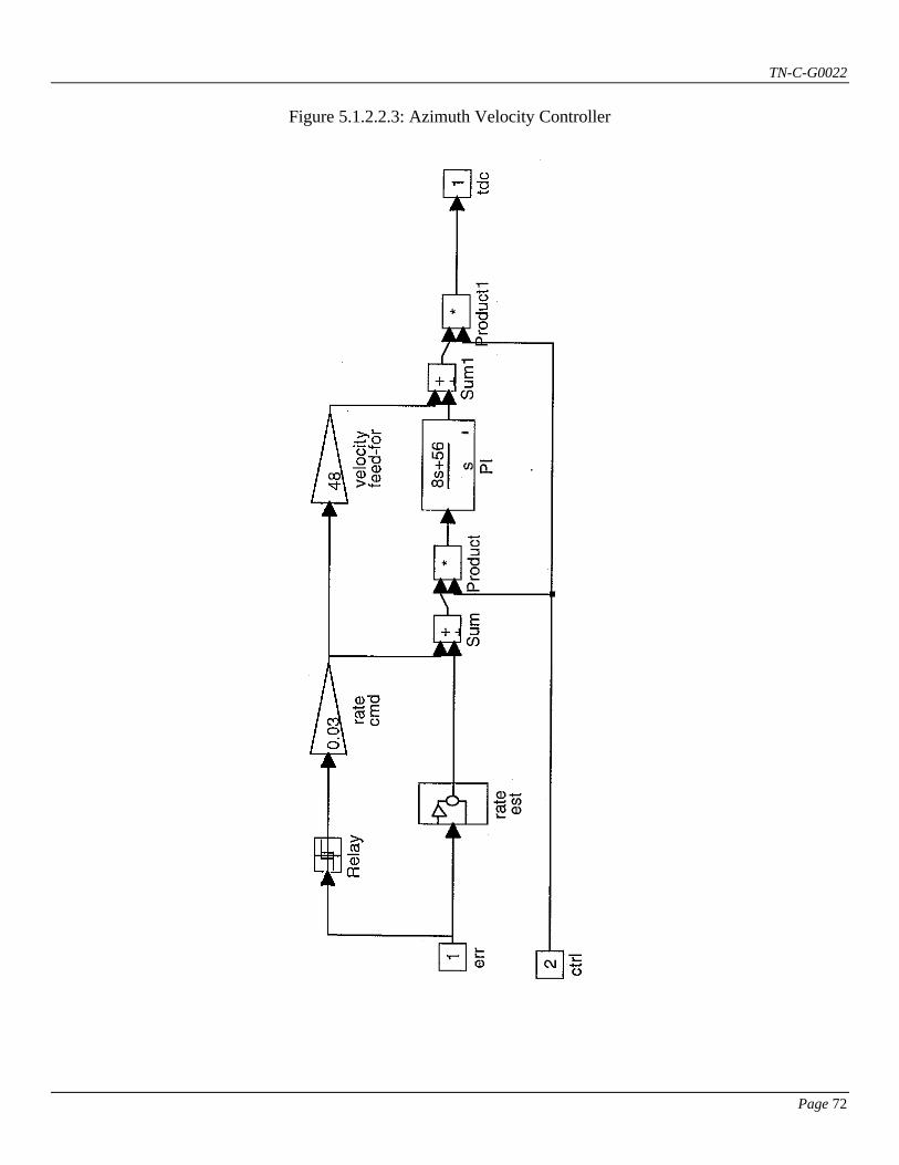
TN-C-G0022

Page 72

Figure 5.1.2.2.3: Azimuth Velocity Controller

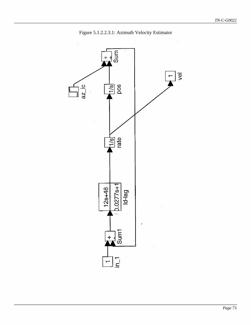
TN-C-G0022

Page 73

Figure 5.1.2.2.3.1: Azimuth Velocity Estimator

TN-C-G0022

Page 74

Figure 5.1.2.2.4: Azimuth Linear Controller

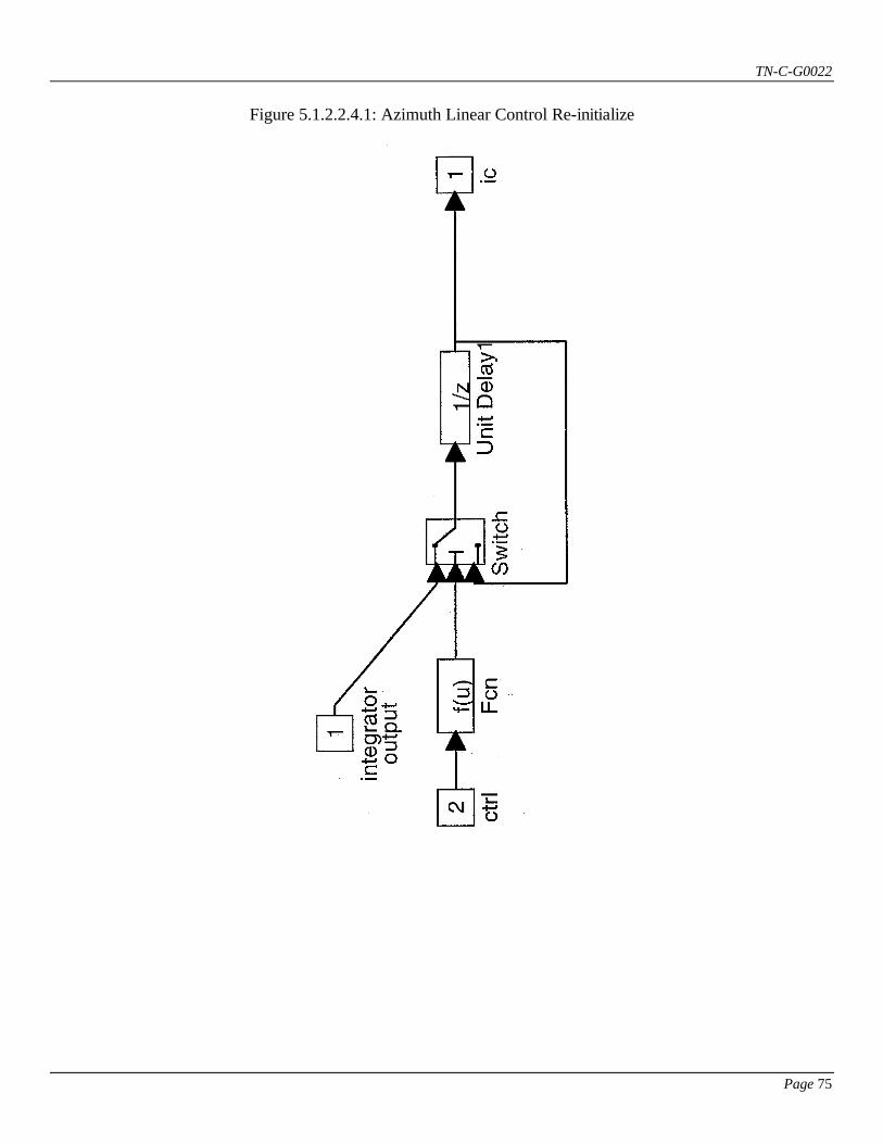
TN-C-G0022

Page 75

Figure 5.1.2.2.4.1: Azimuth Linear Control Re-initialize

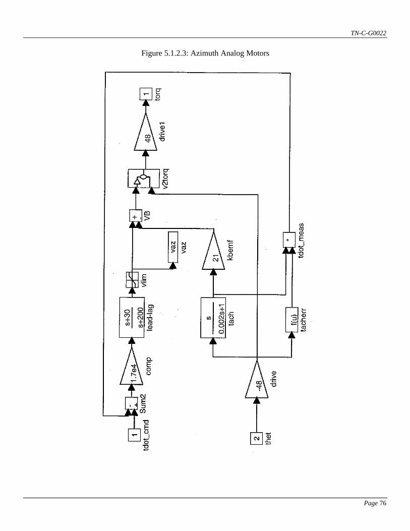
TN-C-G0022

Page 76

Figure 5.1.2.3: Azimuth Analog Motors

TN-C-G0022

Page 77

Figure 5.1.2.3.1: Azimuth Motor Voltage to Torque

TN-C-G0022

Page 78

Figure 5.1.2.4: Azimuth Drive Wheel Friction

TN-C-G0022

Page 79

Figure 5.1.2.4.1: Azimuth Bearing Friction Switch

TN-C-G0022

Page 80

Figure 5.2: Altitude Drive

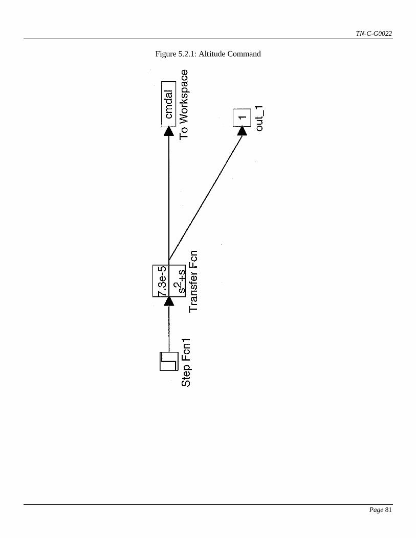
TN-C-G0022

Page 81

Figure 5.2.1: Altitude Command

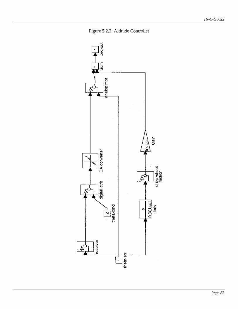
TN-C-G0022

Page 82

Figure 5.2.2: Altitude Controller

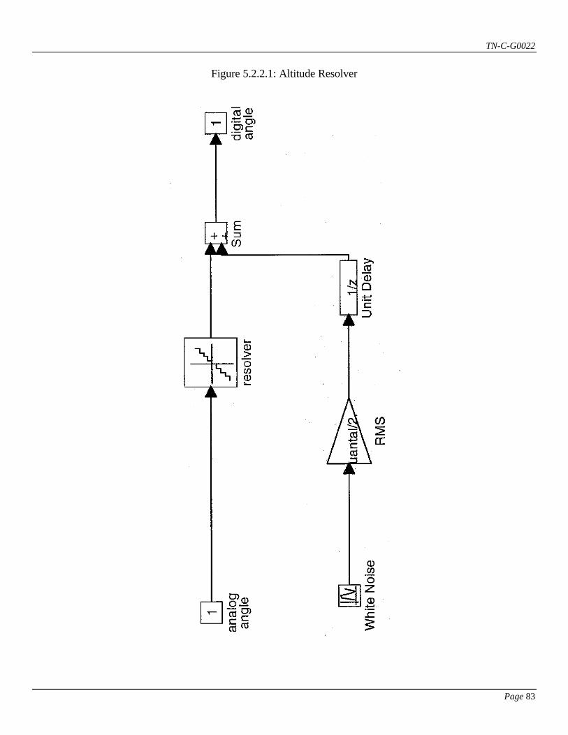
TN-C-G0022

Page 83

Figure 5.2.2.1: Altitude Resolver

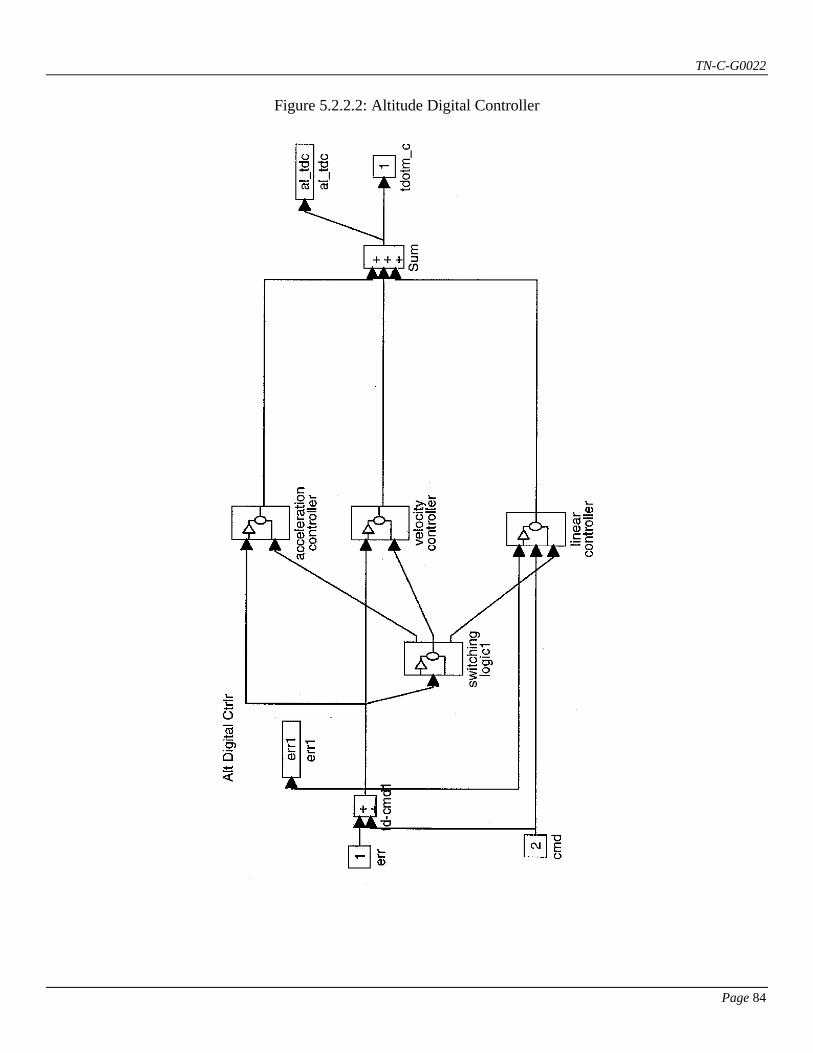
TN-C-G0022

Page 84

Figure 5.2.2.2: Altitude Digital Controller

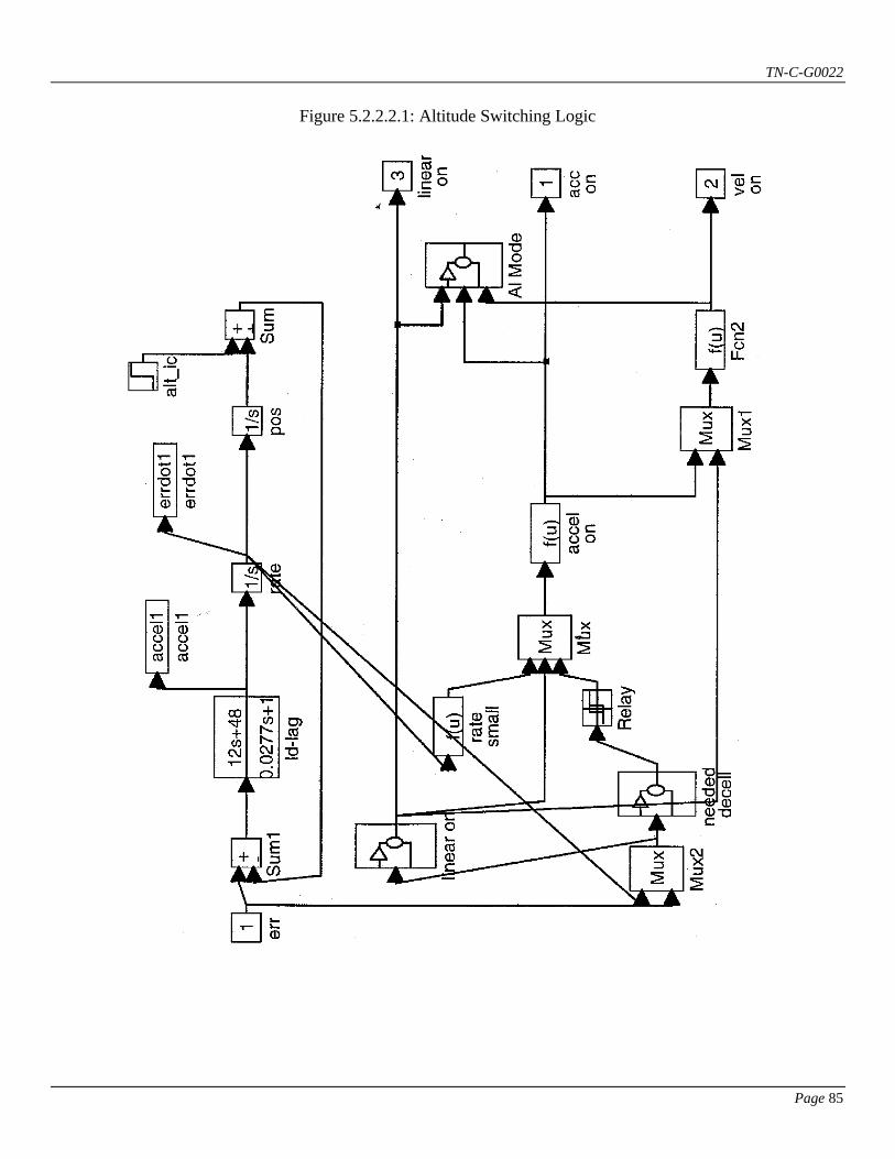
TN-C-G0022

Page 85

Figure 5.2.2.2.1: Altitude Switching Logic

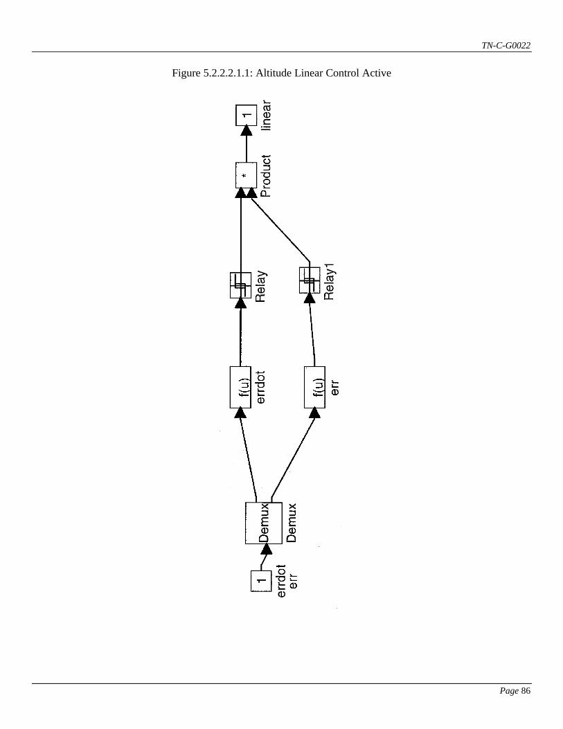
TN-C-G0022

Page 86

Figure 5.2.2.2.1.1: Altitude Linear Control Active

TN-C-G0022

Page 87

Figure 5.2.2.2.1.2: Altitude Deceleration Required

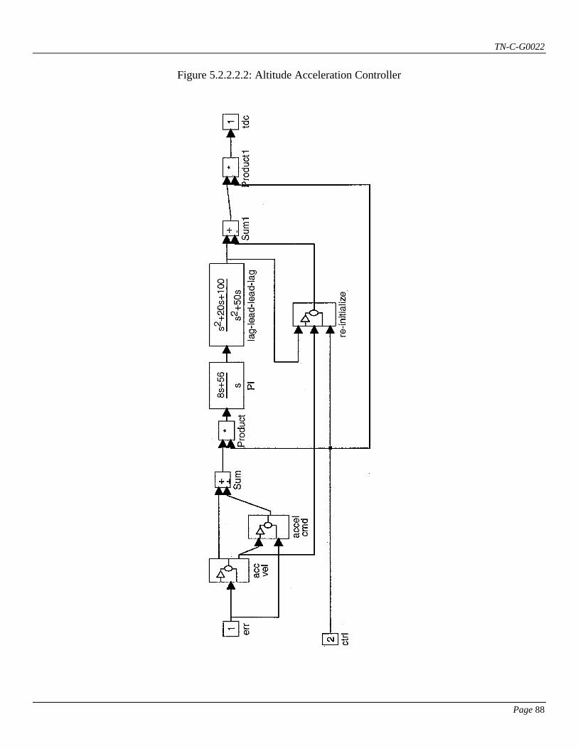
TN-C-G0022

Page 88

Figure 5.2.2.2.2: Altitude Acceleration Controller

TN-C-G0022

Page 89

Figure 5.2.2.2.2.1: Altitude Acceleration Estimator

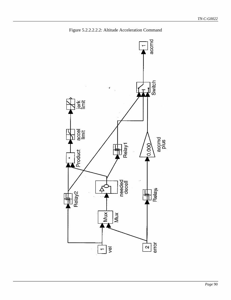
TN-C-G0022

Page 90

Figure 5.2.2.2.2.2: Altitude Acceleration Command

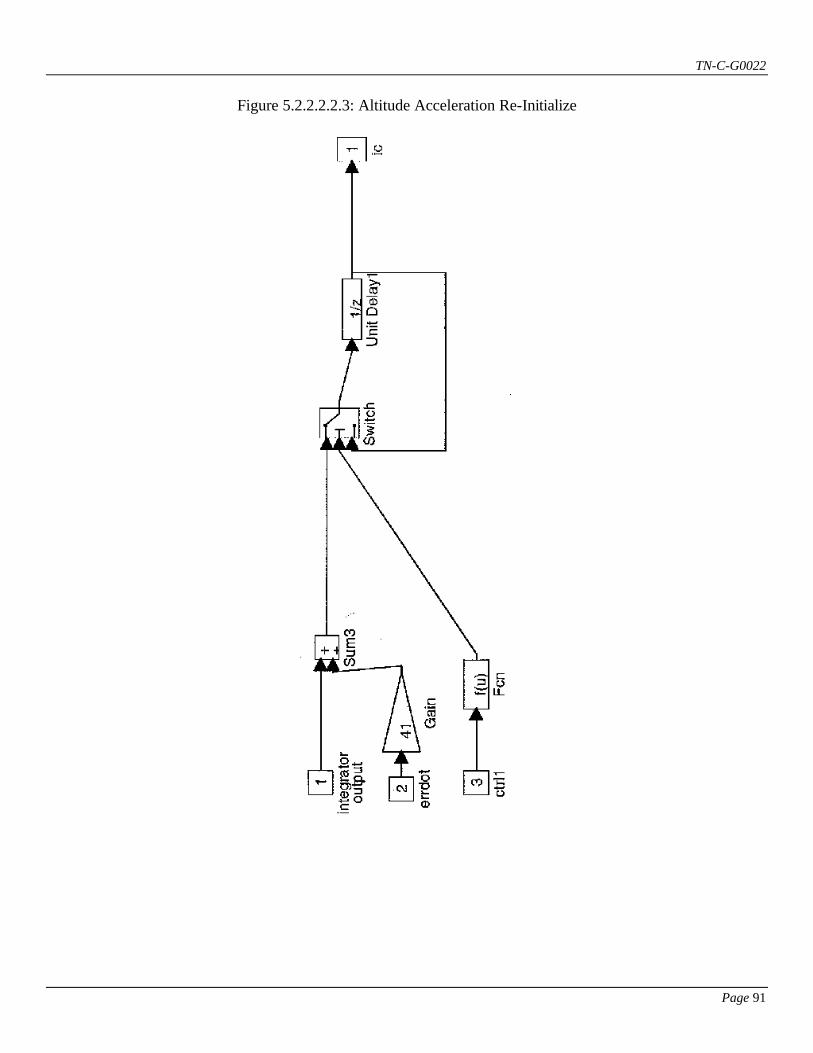
TN-C-G0022

Page 91

Figure 5.2.2.2.2.3: Altitude Acceleration Re-Initialize

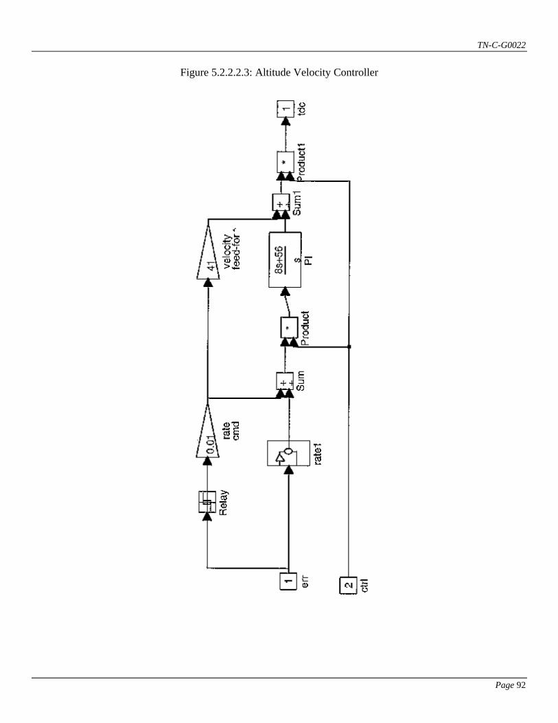
TN-C-G0022

Page 92

Figure 5.2.2.2.3: Altitude Velocity Controller

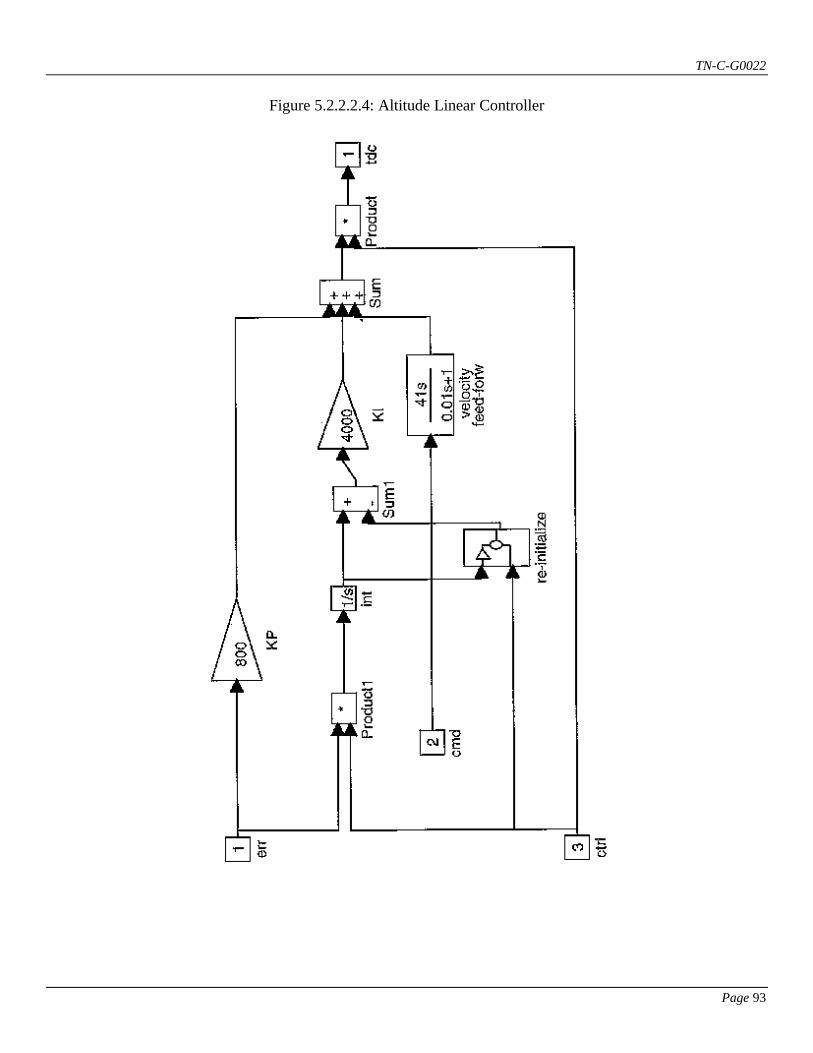
TN-C-G0022

Page 93

Figure 5.2.2.2.4: Altitude Linear Controller

TN-C-G0022

Page 94

Figure 5.2.2.2.4.1: Altitude Linear Controller Re-Initialize

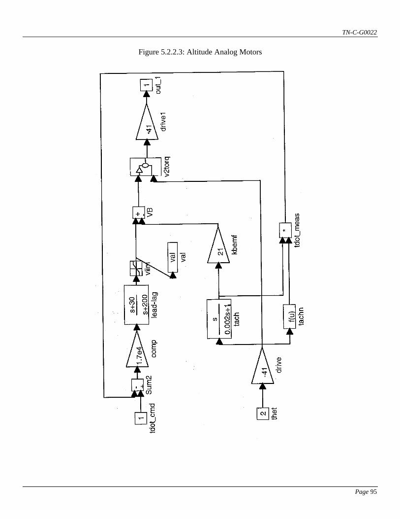
TN-C-G0022

Page 95

Figure 5.2.2.3: Altitude Analog Motors

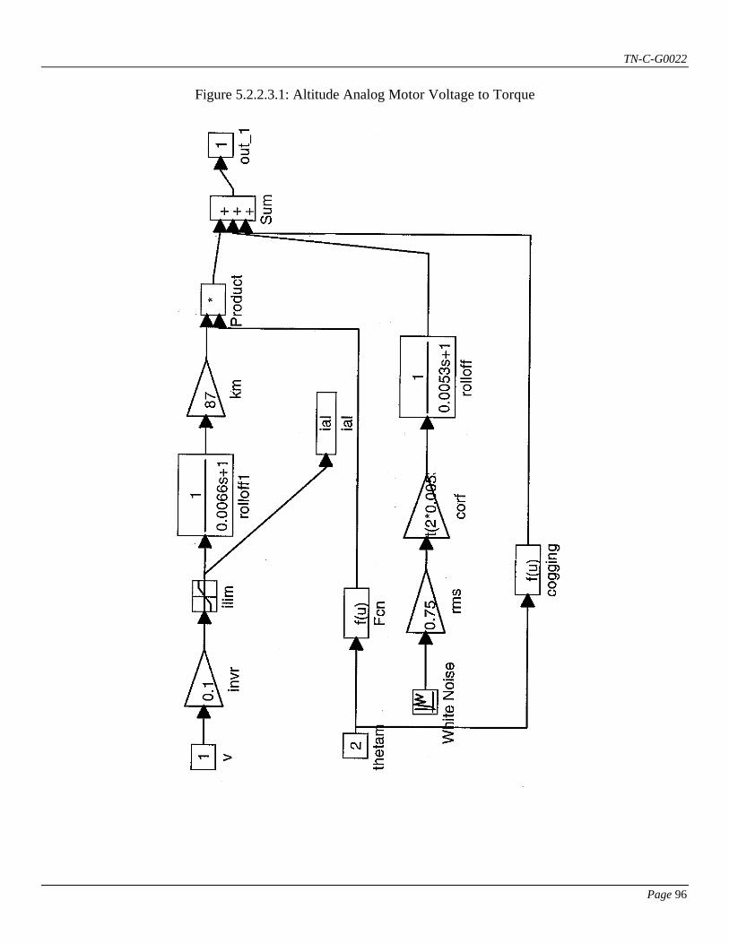
TN-C-G0022

Page 96

Figure 5.2.2.3.1: Altitude Analog Motor Voltage to Torque

TN-C-G0022

Page 97

Figure 5.2.2.4: Altitude Drive Wheel Friction

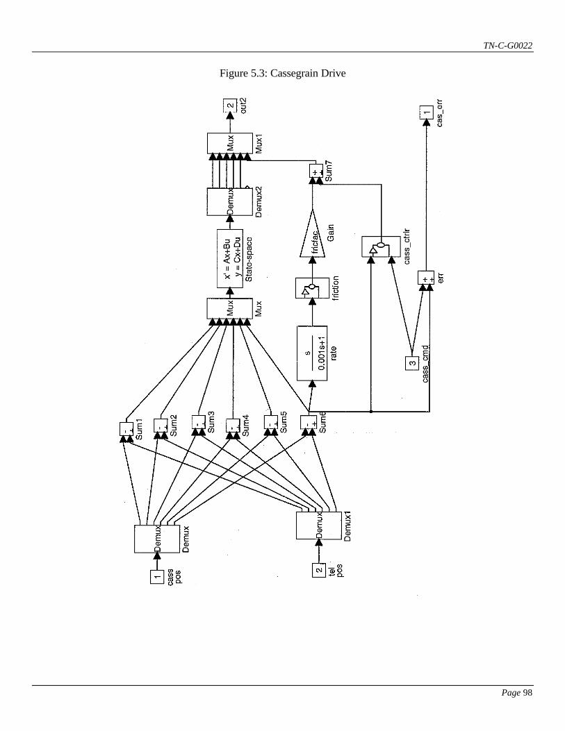
TN-C-G0022

Page 98

Figure 5.3: Cassegrain Drive

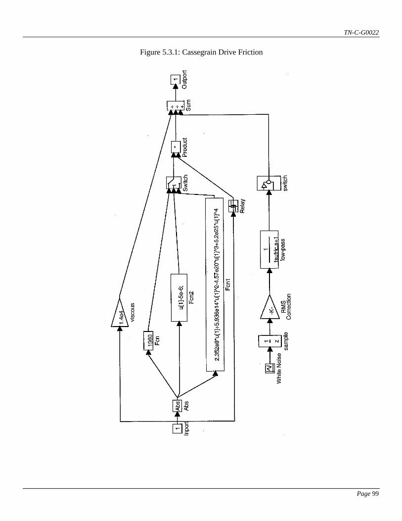
TN-C-G0022

Page 99

Figure 5.3.1: Cassegrain Drive Friction

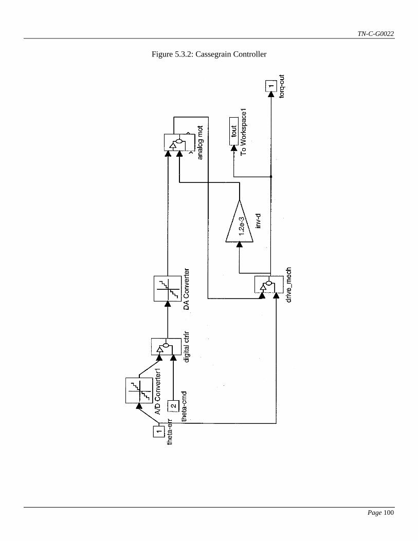
TN-C-G0022

Page 100

Figure 5.3.2: Cassegrain Controller

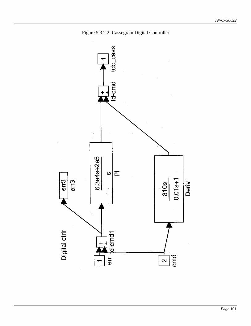
TN-C-G0022

Page 101

Figure 5.3.2.2: Cassegrain Digital Controller

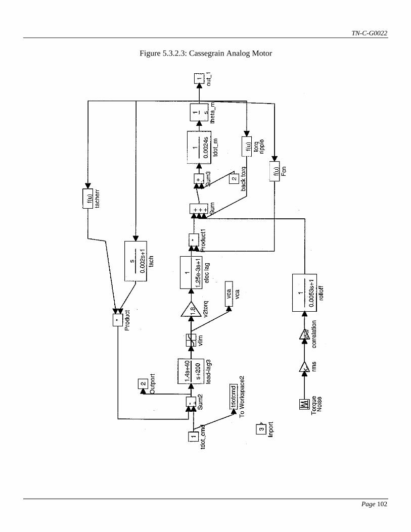
TN-C-G0022

Page 102

Figure 5.3.2.3: Cassegrain Analog Motor

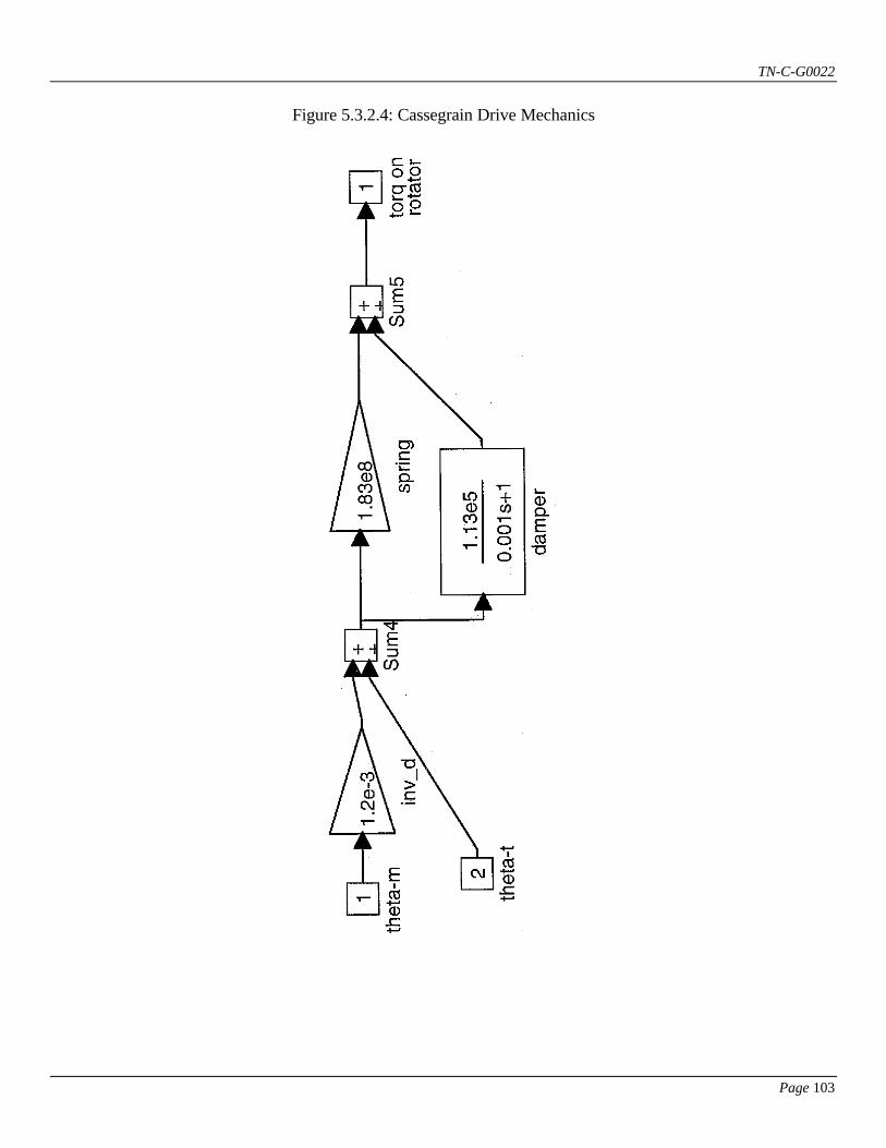
TN-C-G0022

Page 103

Figure 5.3.2.4: Cassegrain Drive Mechanics

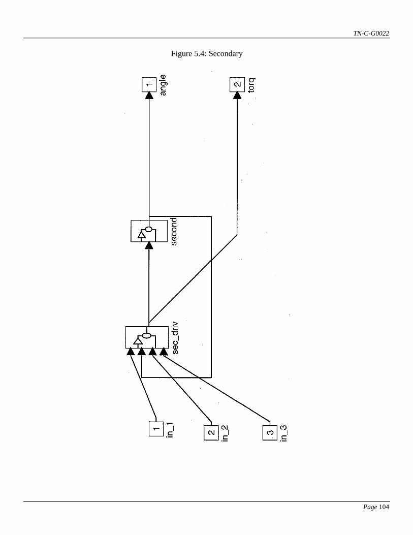
TN-C-G0022

Page 104

Figure 5.4: Secondary

TN-C-G0022

Page 105

Figure 5.4.1: Secondary Drive

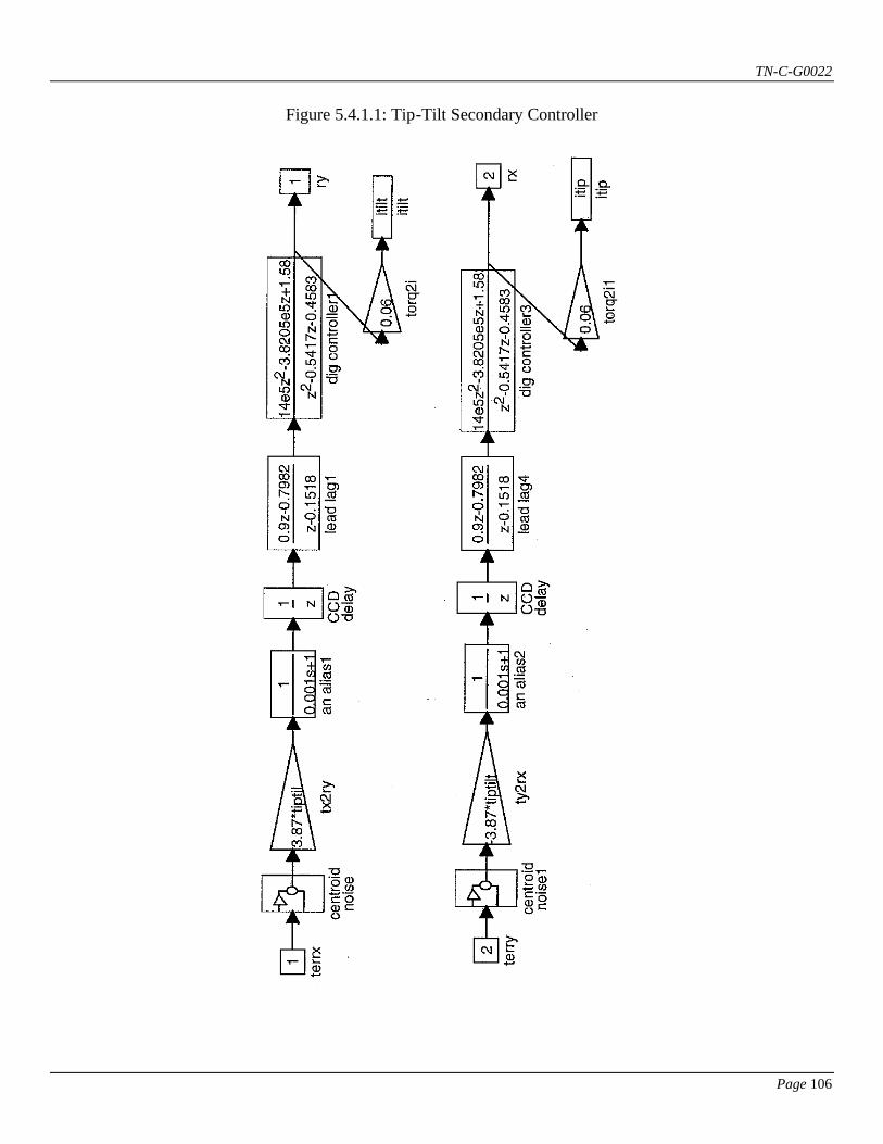
TN-C-G0022

Page 106

Figure 5.4.1.1: Tip-Tilt Secondary Controller

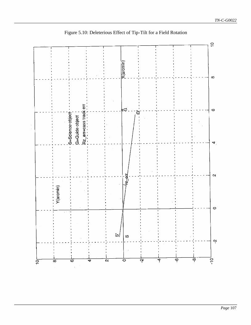
TN-C-G0022

Page 107

Figure 5.10: Deleterious Effect of Tip-Tilt for a Field Rotation

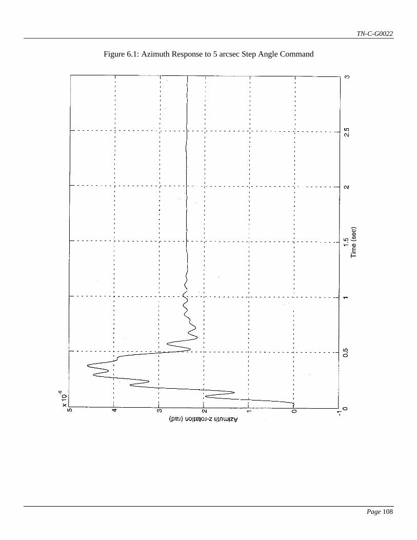
TN-C-G0022

Page 108

Figure 6.1: Azimuth Response to 5 arcsec Step Angle Command

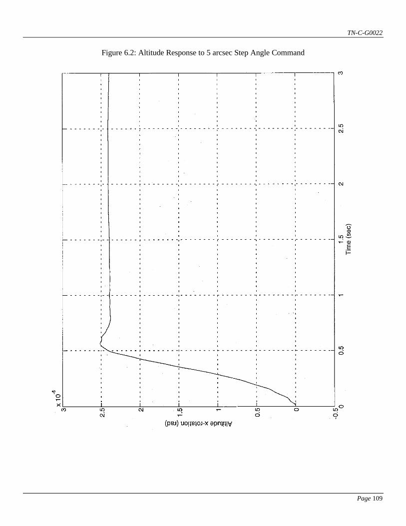
TN-C-G0022

Page 109

Figure 6.2: Altitude Response to 5 arcsec Step Angle Command

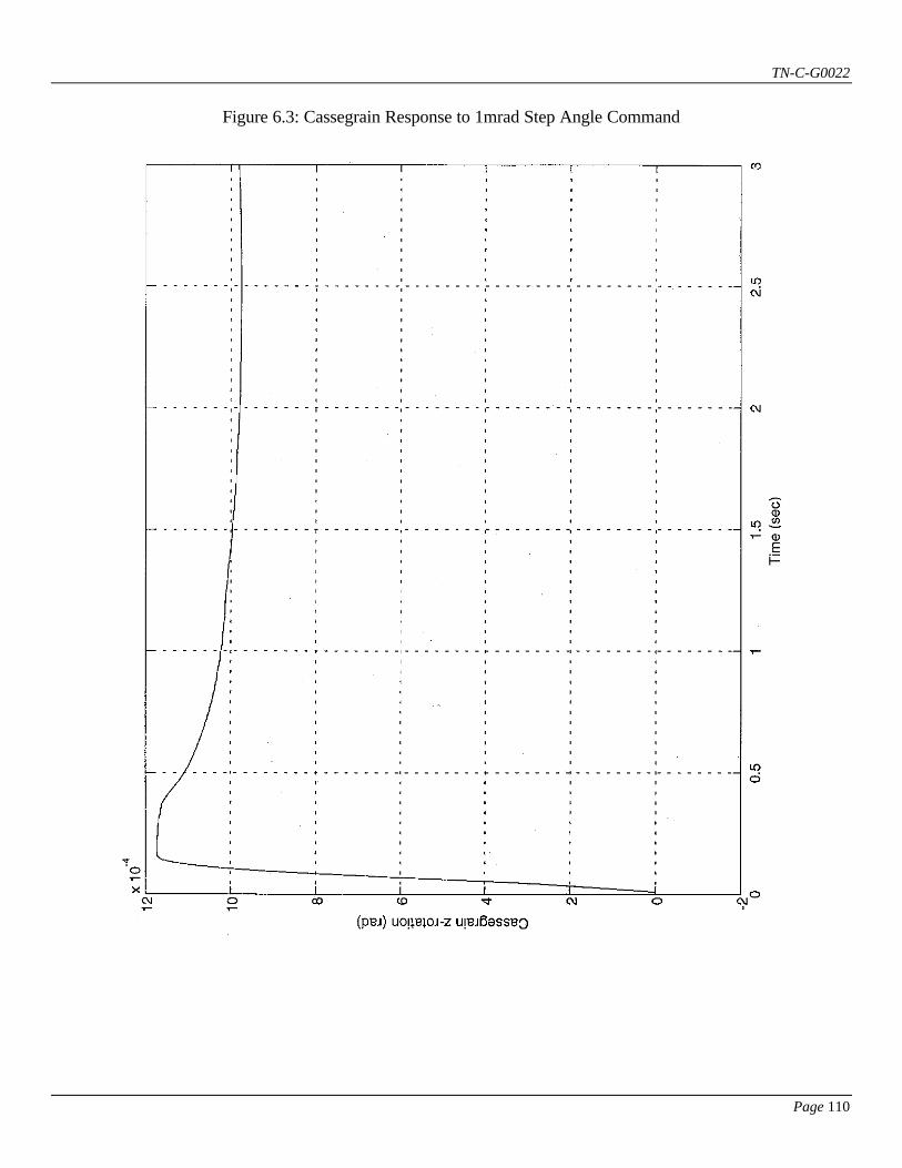
TN-C-G0022

Page 110

Figure 6.3: Cassegrain Response to 1mrad Step Angle Command

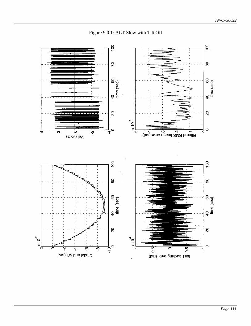
TN-C-G0022

Page 111

Figure 9.0.1: ALT Slow with Tilt Off

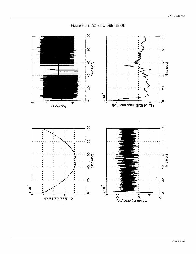
TN-C-G0022

Page 112

Figure 9.0.2: AZ Slow with Tilt Off

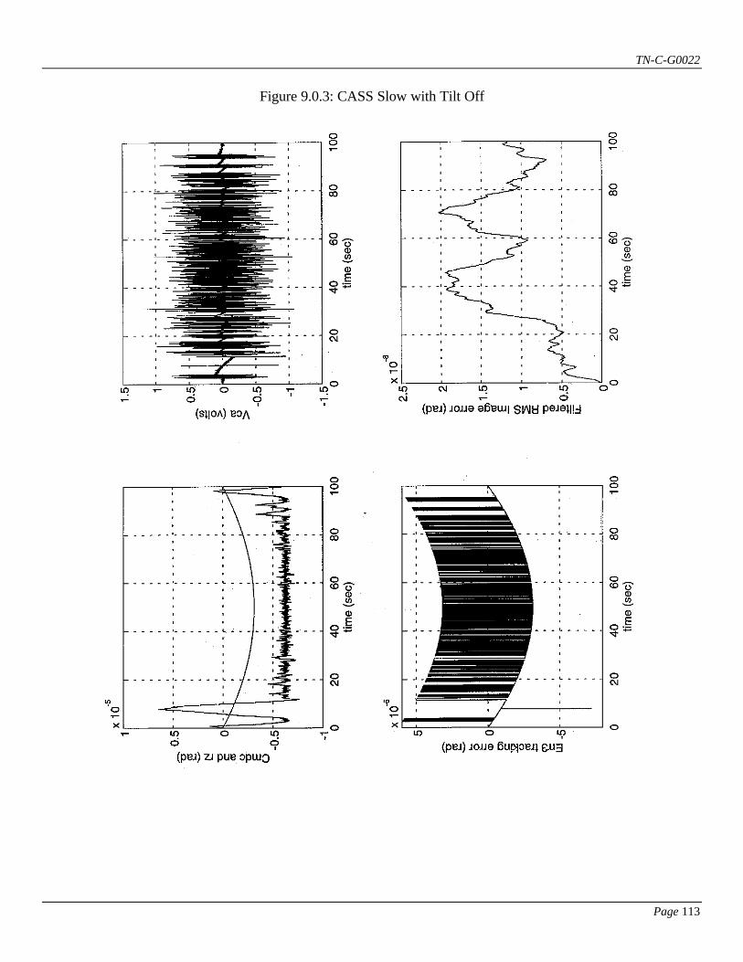
TN-C-G0022

Page 113

Figure 9.0.3: CASS Slow with Tilt Off

TN-C-G0022

Page 114

Figure 9.0.4: ALT Slow with Tilt On

TN-C-G0022

Page 115

Figure 9.0.5: AZ Slow with Tilt On

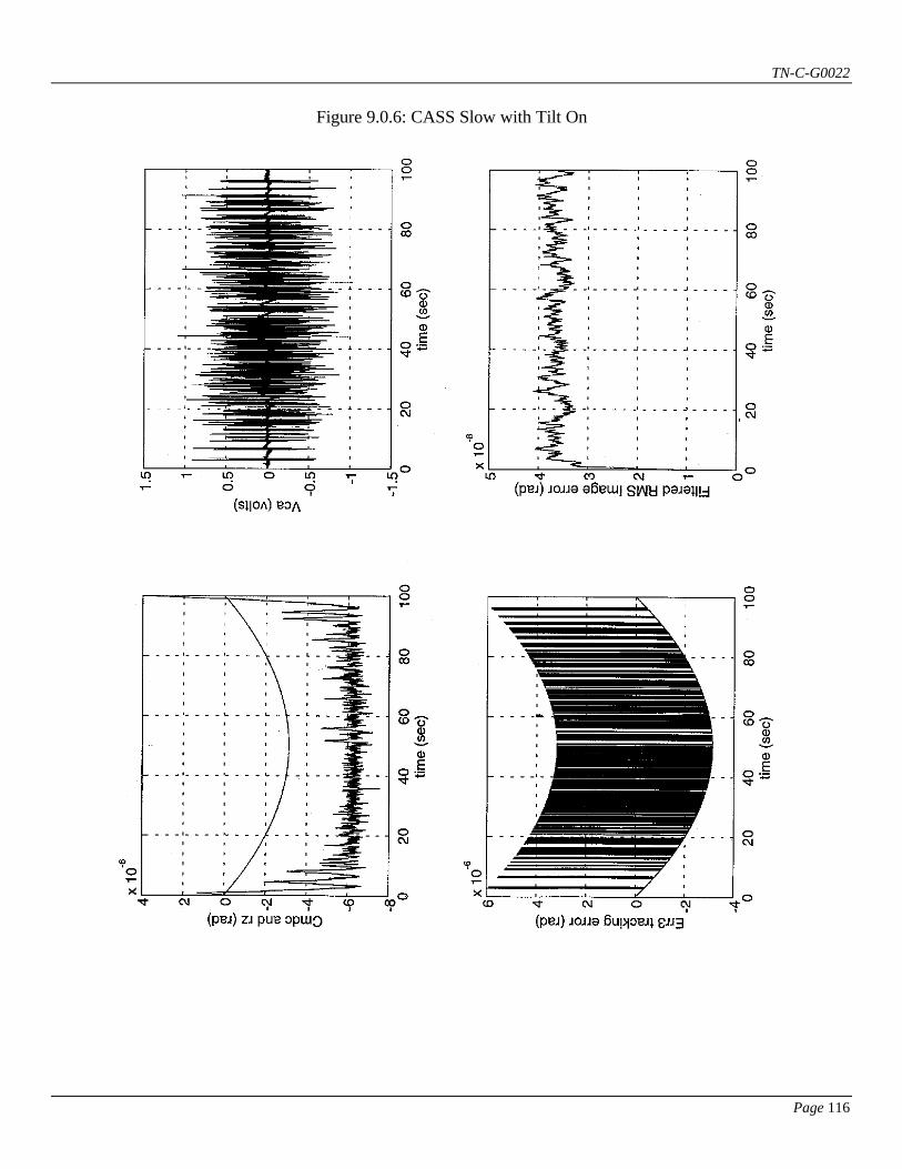
TN-C-G0022

Page 116

Figure 9.0.6: CASS Slow with Tilt On

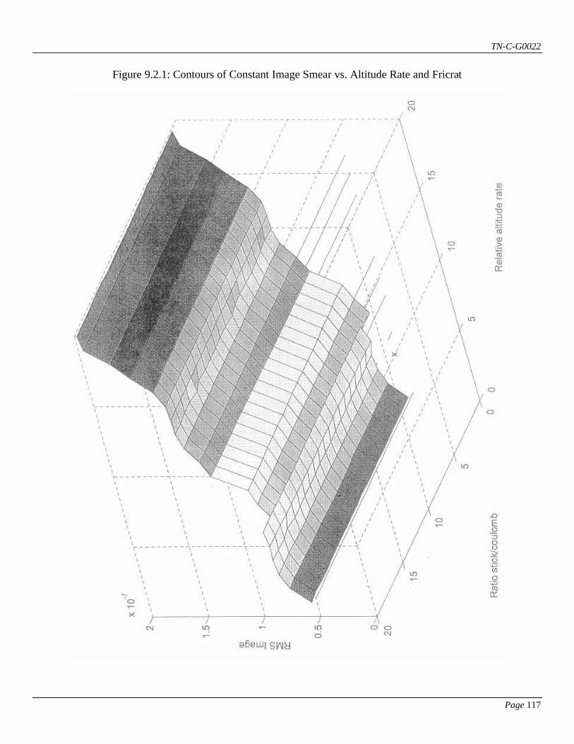
TN-C-G0022

Page 117

Figure 9.2.1: Contours of Constant Image Smear vs. Altitude Rate and Fricrat

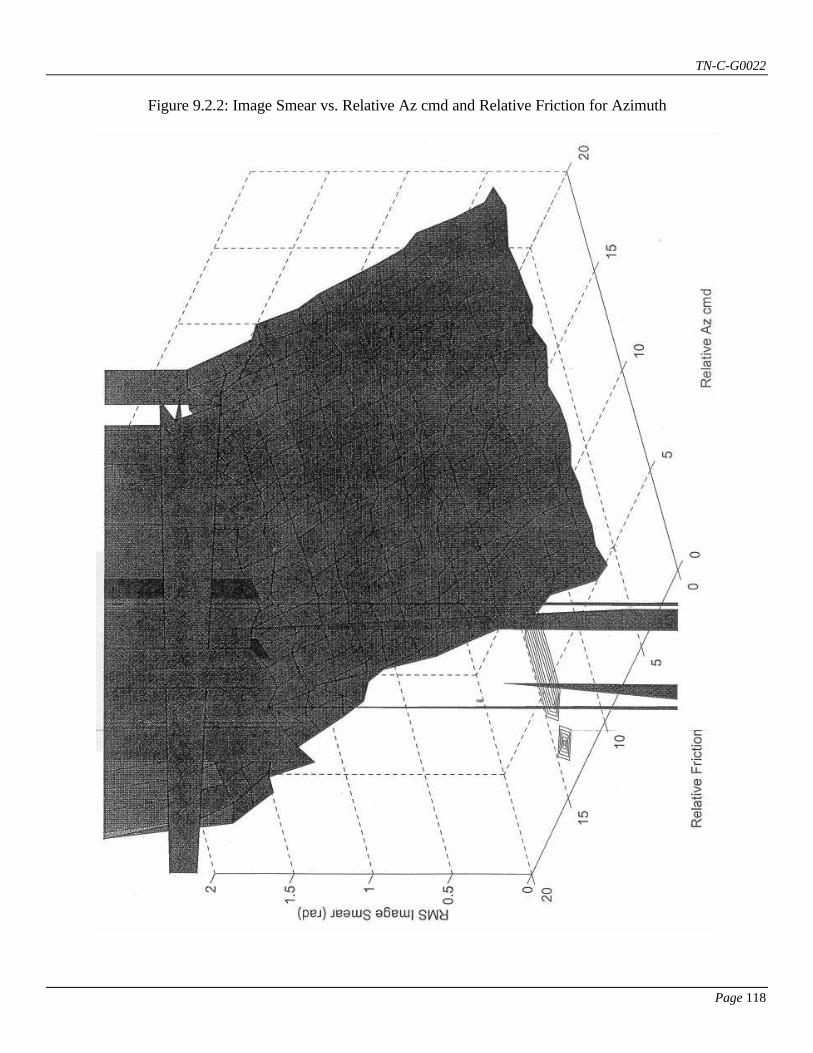
TN-C-G0022

Page 118

Figure 9.2.2: Image Smear vs. Relative Az cmd and Relative Friction for Azimuth

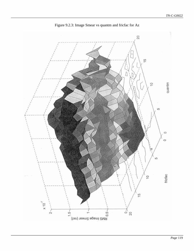
TN-C-G0022

Page 119

Figure 9.2.3: Image Smear vs quantm and fricfac for Az

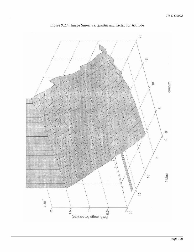
TN-C-G0022

Page 120

Figure 9.2.4: Image Smear vs. quantm and fricfac for Altitude

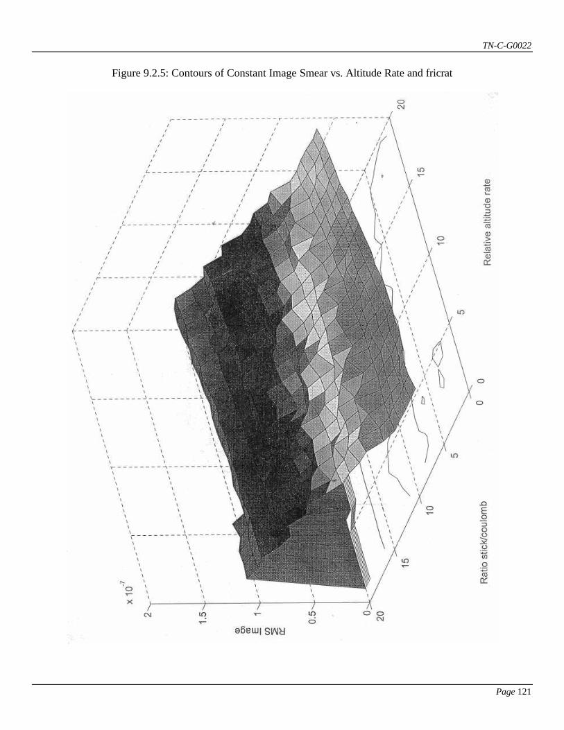
TN-C-G0022

Page 121

Figure 9.2.5: Contours of Constant Image Smear vs. Altitude Rate and fricrat

TN-C-G0022

Page 122

Figure 9.2.6: Image Smear vs quantca and torqnois for Cass

TN-C-G0022

Page 123

Figure 9.2.7: Image Smear vs quantm and fricrat for Alt

TN-C-G0022

Page 124

Figure 9.2.8: Image Smear vs quantm and torqnois for Alt

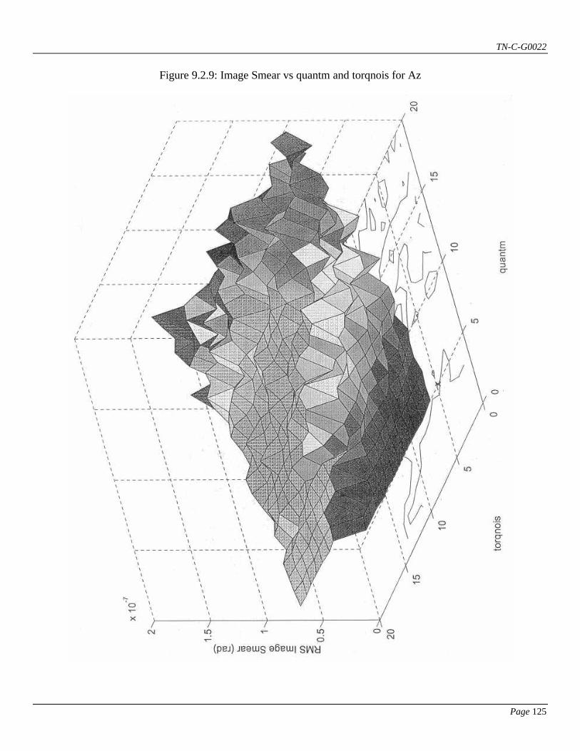
TN-C-G0022

Page 125

Figure 9.2.9: Image Smear vs quantm and torqnois for Az

TN-C-G0022

Page 126

Figure 9.2.10: Image Smear vs fricfac and torqnois for Alt

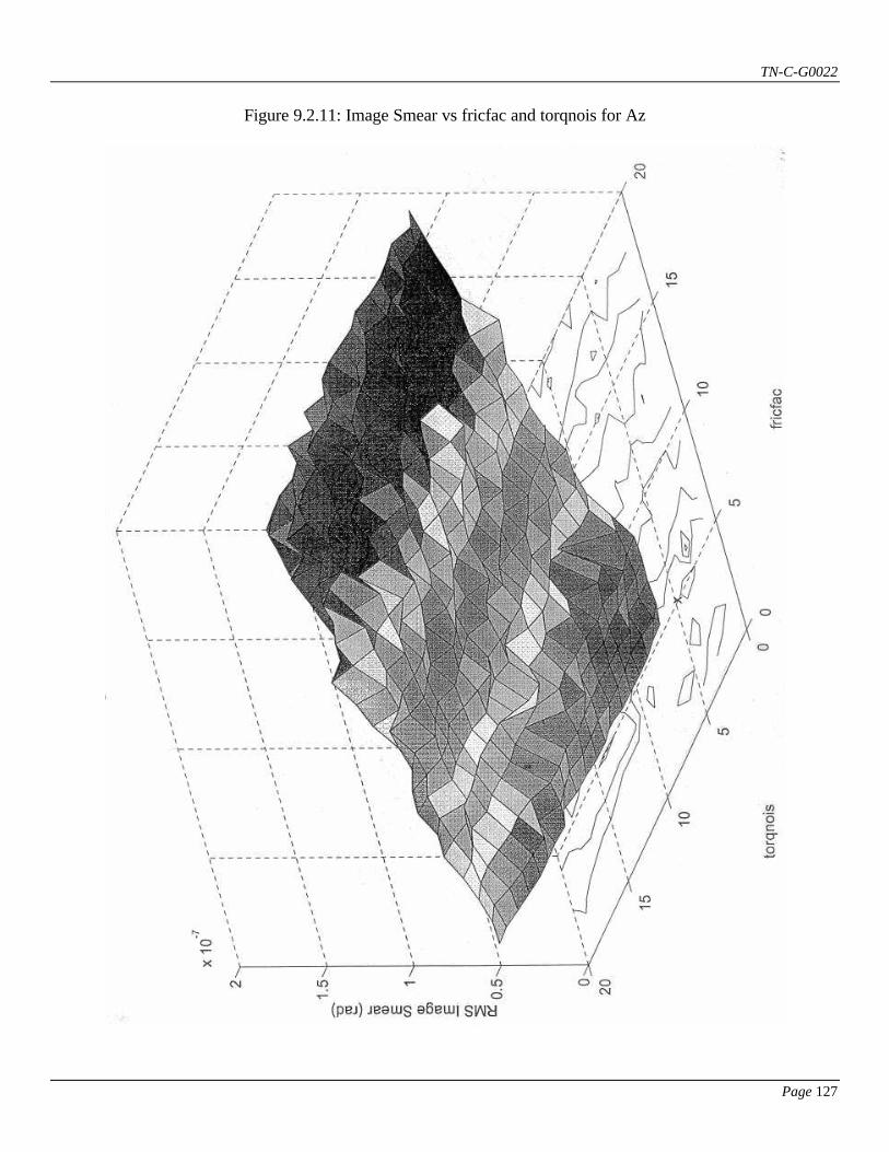
TN-C-G0022

Page 127

Figure 9.2.11: Image Smear vs fricfac and torqnois for Az

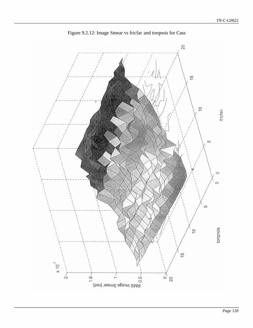
TN-C-G0022

Page 128

Figure 9.2.12: Image Smear vs fricfac and torqnois for Cass

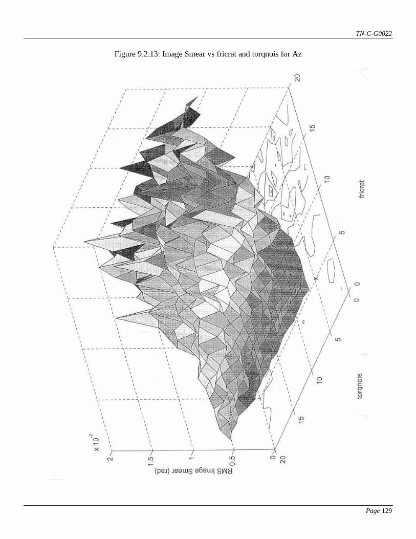
TN-C-G0022

Page 129

Figure 9.2.13: Image Smear vs fricrat and torqnois for Az

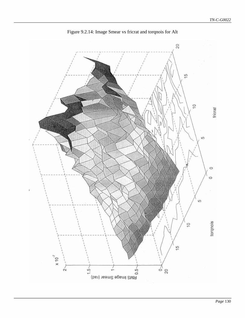
TN-C-G0022

Page 130

Figure 9.2.14: Image Smear vs fricrat and torqnois for Alt

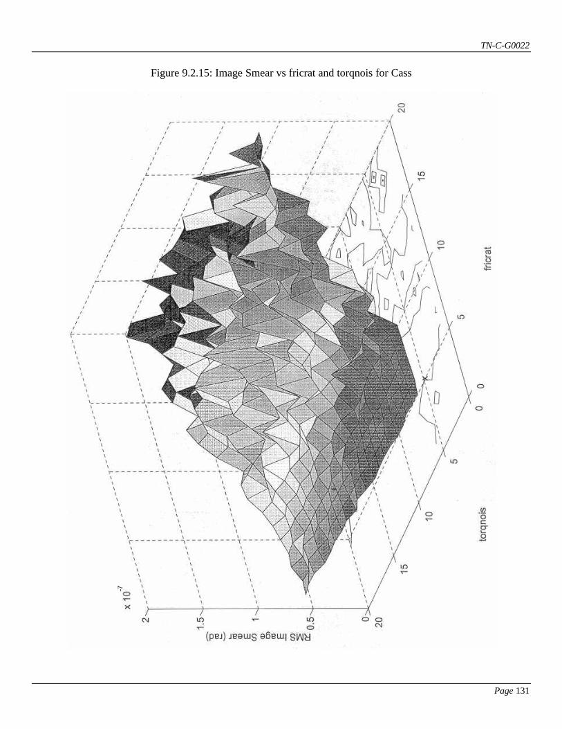
TN-C-G0022

Page 131

Figure 9.2.15: Image Smear vs fricrat and torqnois for Cass

TN-C-G0022

Page 132

Figure 9.2.16: Image Smear vs fricfac and taufric for Alt

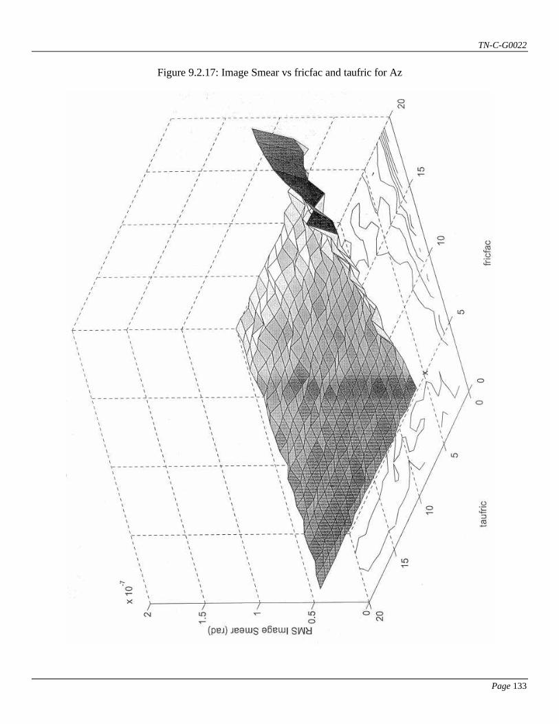
TN-C-G0022

Page 133

Figure 9.2.17: Image Smear vs fricfac and taufric for Az

TN-C-G0022

Page 134

Figure 9.2.18: Image Smear vs fricfac and taufric for Cass

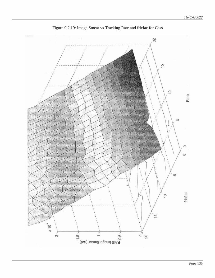
TN-C-G0022

Page 135

Figure 9.2.19: Image Smear vs Tracking Rate and fricfac for Cass

TN-C-G0022

Page 136

Figure 9.2.20: Image Smear vs Tracking Rate and fricfac for Alt

TN-C-G0022

Page 137

Appendices

TN-C-G0022

Page 138

Appendix A1 GEMINI 8-METRE TELESCOPES PROJECT

CONTROLS GROUP _____________________________________________________________________________ To: File Copied To : R. McGonegal From: Mike Burns Date: March 22, 1993 Subject: Tip-Tilt Chopper Control Study and Power Requirements Reference: Power Requirements for Chopper, R. McGonegal , January 17, 1993. Problem It is required that the chopping secondary servo system provide 56.4 arcsecond (=270 micro-rad) motion at a rate of 10Hz. The required settling band of 0.485 micro-rad must be reached in 0.01 seconds to provide a usable duty-cycle of 80%. A candidate controller is developed which meets the requirements and the resulting model is used to estimate the average power. Summary - digital control looks very troublesome at 200 Hz sampling - need 1kHz or more sampling to try digital - continuous control needs 640Hz bandwidth estimator and 75 W net power - summary of power and duty-cycle for various controllers: System Model The basic model of the servo-chopper system is nearly the same as that described in the reference with the addition of some parasitic terms. The calculations of torque and power also have been changed slightly. Figure 1 shows the generalized top-level view of the simulation used for this study. Input is modeled as a 270 micro-rad step that is subtracted from the actual angular position of the secondary to produce an error, labeled Theta-err. The controller block, expanded in Figure 2, acts upon the error to produce a limited command voltage, Vlim, which feeds the servo block of Figure 3. The servo block produces Torque delivered to the Chopper of Figure 4 and an intermediate variable, Ilim, the limited current used by the Power block of Figure 5.

TN-C-G0022

Page 139

The overall simulation is "mixed" in the sense that part of the simulation describes a single actuator and part of the simulation describes the summed effect of 3 actuators. The Controller, Servo, and Power blocks model one actuator, while the Chopper block models the effects of all 3 actuators. The crossover from part to whole occurs in the last gain block of the servo, Figure 3, which is labeled i2trq. The gain i2trq is the scale factor from current in one actuator to net torque produced by 3 actuators. Figure 6 helps to describe the relationship i2trq. Assume that the 3 actuators are placed in the geometry shown and produce forces labeled F1, F2, and F3 Newtons. The desired rotational axis is labeled xx' and the moment arm is z=0.3 meters. The fact that torque is about the xx' axis requires that F2 = F3 . Net force on the mirror must balance, requiring that F1 + F2 + F3 = 0 . Combining the above 2 equations gives F2 = F3 = -F1 / 2 . Noting that sin(30 deg)=0.5, the diagram makes it clear that net torque will be Tnet = F1*z - F2*z/2 - F3*z/2 or Tnet = F1*z + F1*z/4 + F1*z/4 Tnet = F1*z*3/2. For this possible actuator, the relationship between current and force is 35N/A, so the previous equation can be written Tnet = I1 * 35N/A * 0.3m * 3/2 = I1 * 15.8 , showing that the gain i2trq=15.8N*m/A. This is half the value used in the reference but is believed to be more accurate. By way of an argument similar to the one above, the net power may be shown to be 1.5 times the power in the actuator number 1. Note that an alternate geometry would be to draw the axis of rotation through one of the actuators in Figure 6. It is not shown here, but the resulting i2trq=18.2. The 15.8 value is chosen because it is the more pessimistic (hitting the current-limit and torque-limit sooner). In general, the geometry would influence controller gains between these extremes.

TN-C-G0022

Page 140

The Servo block of Figure 3 also shows two other small changes from the referenced memo: addition of a back-EMF term and an electrical time constant, taue=0.25 milli-seconds. A first guess at the controller model is to use the PID controller of the reference. Note that gains appear doubled because this controller goes from theta-err to volts, whereas the reference went from theta-err to current. Current and voltage are related by the 2 ohm armature resistance. The derivative term of the controller is changed from a pure differentiator to one with a very small time-constant, taud=0.3ms to reflect the lag inherent in measuring or calculating speed. The controller also includes a voltage limiter which was not modeled in the reference, but is always part of a power amplifier which will drive the servo. Note that the current limit is also modeled, but is not sufficient. Roughly, the current limit restricts net force and voltage limit restricts rate of change of force. The chopper of figure 4 is fundamentally unchanged from the reference, and the Power block integrates I*I*R and divides by the 0.05sec half-wave time to get average power. To summarize, the basic model used in this study is the same as that of the referenced memo except for the following changes: - i2trq changed from 31.5 to 15.8 N/A - voltage limiting - back EMF in servo - servo dynamic time constant of taue=0.25 ms - controller differentiator time constant, taud=0.3 msec. SIMULATION RESULTS AND THE SEARCH FOR A GOOD CONTROLLER Original PID-Benign case Figure 7 shows simulation results for the most benign possible case, omitting voltage limiting, omitting back EMF, omitting servo electrical time-constant, and having negligible (0.03 ms) differentiator time-constant. The measured outputs are from top to bottom: Theta-error (rad), servo voltage (V), servo current (A), mirror angle (rad), angular rate (rad/sec), and average power (W). Figure 8 redraws the error on a better scale and shows that the spec is met since error falls below 0.485 micro-rad before 0.01 sec. Despite the integral term, the MatrixX implementation of this PID controller has a non-zero steady state error. This error is likely due to quantization effects within MatrixX or to the very tiny integral gain which causes an error to be reduced only very slowly. The resulting power is 5.1 W . Original PID-with parasitics Figures 9 through 18 show the effects of adding gradually more of the parasitic effects. The voltage limit and back-EMF have little effect on power, perhaps reducing power marginally, and make the system slightly slower such that the 0.485 micro-rad settling band is not reached until

TN-C-G0022

Page 141

0.012 sec. The addition of an electrical time-constant has increases power consumption 40% to 7 W. The most devastating effect upon power comes from the controller differentiator lag, taud. Increasing it to 0.1 ms then to 0.3 ms increases power to 9.5 W and 20W. If taud is increased to 1ms, the controller is hopeless, with power increasing to 65W and settling time going to 0.04 sec. Taud=0.3 ms was chosen rather arbitrarily as a good representative value of a realistic sensor without greatly harming performance. PID-increased gain Can the structure of this controller be saved and adequate performance restored by changing gains? The root locus plots of Figures 19-24 help in describing this system. The first 3 of these figures show the root locations of the benign system for changing the proportional, integral, and derivative gains by the scale factors shown on the plots. It is interesting to note that the integral gain may be changed by a factor of 20 while moving the root location negligibly. This indicates that the original controller was nearly a PD type. Since the derivative time constant, taud, was the most important of the parasitic elements modeled, its root locus is shown in Figure 22. Predictably, things get much slower for taud=0.3 ms than for 0.03 ms. Figures 23 and 24 show the proportional and derivative root loci again, this time for the less benign case of taud=0.3 ms. Increasing either the P or D gain improves the root on the real axis near -400 at the expense of the lightly damped root near 400 +j1600. Increasing the P gain by a factor of 1.5 seems to give the best tradeoff, with time responses shown in Figures 25 and 26. The settling time has been restored to near 0.0105 sec but power has increased to near 32 W. Digital control Thus far only a continuous time controller has been modeled, but in the actual system there are strong reasons for using a digital controller, notably ease in changing parameters and stability of coefficients. Figure 27 shows the root locus of the discretized system with a 200Hz sampling rate and an extra step delay to represent computational lag. Figure 27 was found to be poor because of the root near -0.8 at the left of the plot tending to go unstable as gain increased. Figure 28 shows the effect of adding a lead-lag compensator to pull in the errant pole. Still the system response of Figure 29 is poor. Note that at 200Hz the controller has precisely 2 steps in which to reduce the system error by a factor of 0.0018 (from 270 to 0.485 micro-rad), so the effective system root must be near sqrt(0.0018)=0.04 . This is so close to deadbeat as to likely be unattainable with a linear controller, so a bang-bang type controller was examined for the first two steps handing off to a slower linear controller to maintain good noise response. Figure 30 shows the MatrixX block diagram of a controller which was cascaded with the linear digital controller to implement the bang-bang function over the first two time steps. The bang-bang control used here is slightly more sophisticated than that described in the reference in that the chopper is modeled as inertia-spring-damper rather than merely inertia. Following are a few words about derivation of the control steps. The chopper may be represented by the discrete state space equation

TN-C-G0022

Page 142

x(k+1) = PHI * x(k) + gam * u(k) where x(k) is the state [theta(rad) theta-dot(rad/sec)]' and u(k) is the applied torque. It is desired to find torques u(0) and u(1) such that the system is moved from its original state x=[0 0]' to the state [2.7e-4 0]' . The state space equation may be iterated to give x(1) = PHI * x(0) + gam * u(0) x(2) = PHI * PHI * x(0) + PHI * gam * u(0) + gam * u(1) . The last equation above is a simple linear equation in the unknowns u(0) and u(1) and may be rearranged and solved: x(2) = PHI * PHI * x(0) + [PHI * gam | gam ] * [u(0) u(1) ] ' or inv[PHI * gam | gam] * [x(2) - PHI*PHI*x(0)] = [u(0) u(1)] . Solving the above gives the necessary step torques of u(0)=43.618 Nm and u(1)=-41.321Nm. This is quite close to the simpler values derived in the reference of +/- 43.68 Nm, showing that inertia is much the dominant term. Neglecting the effect of the electrical time constant, the computed torques correspond to commanded voltages of 5.521V and -5.231V respectively. Unfortunately, when these are applied to the system the effect is completely unsatisfactory as shown in Figure 31. The large transient response in theta-err is due to the neglected state associated with the electrical time constant. Figure 32 verifies that the system response is excellent, with theta-err=0.03 micro-rad, when the electrical lag is removed. One could rewrite the state equations to include the effect of the electrical lag, but it would require at least 3 time steps to move all three states to the arbitrary location, violating the 0.01 sec required settling time. In general an N-state system will require N steps to move from one state to another specified state. Even if we were to build a controller that would take into account the known states, unmodelled states would remain which would cause harm analogous to that shown above. One would still need a fast linear controller to take out the system error. For example, with a 1kHz sampling rate, one would have 10 steps in which to remove error. The first 3 steps could be used to take out the 3 known states and the other 7 steps could remove the remaining error due to unmodeled effects. Due to actuator current limit, and thus torque limit, 3 steps might be insufficient time in which to move the system. In such a case more steps could be used or the effective torque limit could be increased by including 4 or more actuators in a different geometry. A 1kHz digital filter should easily be implementable on the current system. For an n-state filter, there are required roughly n^2+3n floating point multiplies and as many floating point adds. So a 5 state filter would need approximately 40 multiplies and 40 adds. Assuming a 68030 processor operating at 25MHz, there are 25,000 clock cycles in a 1ms sample time. Conservatively estimating that a floating point multiply takes 64 clock cycles and an add takes 44 clock cycles gives a total of 4,000 clock cycles for the filter. Doubling this to 8,000 clock cycles to

TN-C-G0022

Page 143

conservatively estimate the necessary software overhead still uses only 1/3 of the available CPU power. Kalman Filtering/Optimal Control Since the above analysis shows that a 200Hz digital system has little hope of working, a Kalman-filtering/optimal-control type approach was considered in the continuous domain. Figure 33 shows the resulting system with the estimated states being chopper-angle, angle-rate, and servo-current. Properly speaking, the system shown is neither Kalman-filtering nor optimal-control because the estimator gains ke and controller gains kc are not chosen based on measurement or system noise. Still, the structure is the same. Figures 34 and 35 show the time responses associated with the first iteration of this approach, with controller gains which give poles at -1000 and -700 +/-j714 and estimator gains which give poles at -2000 and -1400 +/-j1428. The transient response is seen to die out quickly enough in 6 ms, but there is left a steady-state error of 1 micro-rad, well above the specified 0.485 micro-rad. One alternative is to add another state, integrated error, and redo the filter and controller gains for the resulting 4-state system. A more simple approach was taken in just making the controller stronger. Figures 36 and 37 show the effect of moving the controller poles to -2000 and -1400 +/-j1428 and the estimator poles to -4000 and -2800 +/-j2828. Now the steady-state error is only 0.25 micro-rad. If this steady-state error were unacceptable, one could cascade the limited PI controller of figure 38. The limiter before the integrator insures that it will not become highly charged by the initial violent transient and will only affect the long term response as shown in Figures 39 and 40. The estimator pole at -4000 rad/sec is equivalent to a bandwidth of 640Hz which should easily be implementable. Notes on Scaling All of the controllers presented here are likely to have a much easier time at a slower chopping rate. Since every controller has an initial transient response similar to bang-bang, it seems reasonable to consider the equation from the reference: T^2 = 4 * theta * J / torq where T is the travel time, theta the angle to be traversed, J the moment of inertia, and torq the maximum torq. Assuming that most of the power is used in the initial transient and letting "~" represent "is proportional to" the following dependencies are noted: Pav ~ Pmax ~ current^2 ~ torq^2 ~ 1/T^4 ~ theta^2 . So for example with a 5Hz chopping rate and a 540 micro-rad angle, the net effect is that power is reduced by a factor of 4. Note that this assumes that the torq limit (current limit) is similarly reduced for the slower chopping case. For those controllers which meet the required settling time this would be allowable. The response could be speeded up by allowing a comparatively larger torque limit at the expense of more power, offering hope for some of the slower controllers which barely missed meeting the settling time.

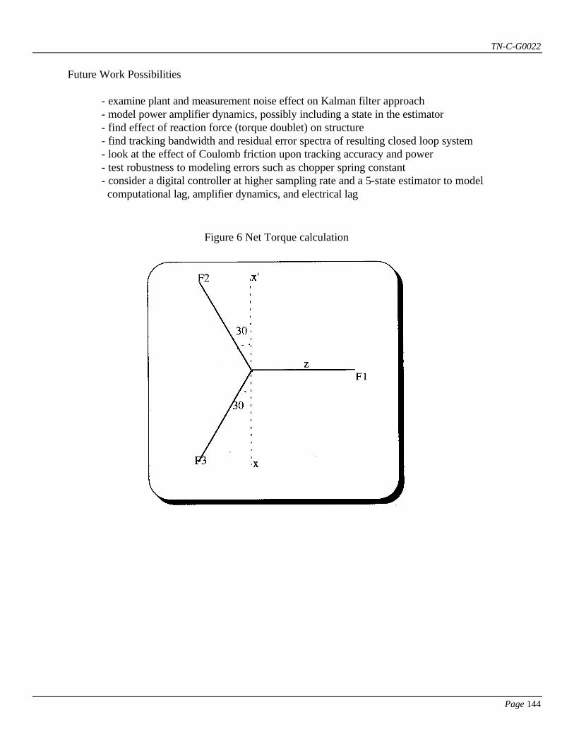
TN-C-G0022

Page 144

Future Work Possibilities - examine plant and measurement noise effect on Kalman filter approach - model power amplifier dynamics, possibly including a state in the estimator - find effect of reaction force (torque doublet) on structure - find tracking bandwidth and residual error spectra of resulting closed loop system - look at the effect of Coulomb friction upon tracking accuracy and power - test robustness to modeling errors such as chopper spring constant - consider a digital controller at higher sampling rate and a 5-state estimator to model computational lag, amplifier dynamics, and electrical lag

Figure 6 Net Torque calculation

TN-C-G0022

Page 145


CONTROLS GROUP _____________________________________________________________________________ To: File Copied To: R. McGonegal From: Mike Burns Date: April 8, 1993 Subject: A Method for Determining Tip-Tilt Secondary Bandwidth and Power Requirements Reference: [1]Bandwidth and Power Requirements for Tip-Tilt, R. McGonegal , January 17, 1993. [2]Power Requirements for Chopper, R. McGonegal, January 17,1993. [3]Tip-Tilt Chopper Control Study and Power Requirements, M. Burns March 22, 1993. Problem It is required to have a tip-tilt secondary mirror system which tracks out 90% or more of the power associated with atmospheric noise on a stars apparent motion. The resulting system must be tolerant of a reasonable number of sample delays and boxcar averaging steps and have acceptable gain and phase margins. Summary Two models of atmospheric noise are considered, the first being the Greenwood model of ref [1] and the second a modified version of the Greenwood model having significant energy at higher frequencies. For the former and more benign case, bandwidth of 5 Hz is sufficient to meet the noise rejection criterion. Achieving a phase margin of 70 degrees pushes the sampling rate requirement to 1Khz to be able to tolerate 5 delays and 5 boxcar averaging steps. For the modified Greenwood noise model, a 15Hz bandwidth servo system is required to reject 90% of the noise. A sampling rate of 1Khz gives a phase margin of 66 deg for 3 delays and 3 boxcar averaging steps. A lower sampling rate would result if the phase margin requirement were relaxed, but this is not recommended since unmodelled delays and lags could greatly degrade performance by pushing the servo loop into a region of excessively light damping or even instability. Both noise models require less than 1 micro-watt of actuator power. These simulation runs can be repeated when we settle on a believable model of the wind.

TN-C-G0022

Page 146

Noise Model: Greenwood Figure 1 shows the power spectral density (in rad^2/Hz) of the Greenwood type noise process as represented in the reference [1]. This power spectrum can be represented in terms of the normalized frequency x=f/f0 as x^(-2/3) H(x) = --------------- for x < 0.332 (2*pi)^2 x^(-2/3) * (1.12-0.361*x) H(x) = ---------------------------------- for 0.332<x<3.1 (2*pi)^2 = near zero for 3.1< x , where f0= v/(pi*D) . The un-normalized power spectrum , in rad^2/Hz is F(f) = H(x) ----------------------------------- 0.481*f0*(r0/D)^(5/3) * (D/lam)^2 where v = velocity of seeing layer = 20 m/s r0 = aperture = 1000 mm D = mirror diameter = 8000 mm lam = wavelength of interest =0.0022 mm . Thus f0 is found to be around 0.8 Hz. The above spectral density, F(f) is referred to as the Greenwood spectral density in this report. Noise Model: Modified Greenwood A better approximation to the atmospheric noise is to let the tail at higher frequencies fall off like f^(-11/3) rather than being considered negligible above the cutoff frequency of 3.1*f0=2.5Hz. Though it still falls off quite quickly, it will be shown that the total energy in this tail is significant both because it extends over a broad frequency range and because it is

TN-C-G0022

Page 147

that part of the spectrum over which we have poor disturbance rejection. The resulting spectrum is referred to as the Modified Greenwood in this report. Thus: x^(-2/3) H(x) = --------------- for x < 3.1 (2*pi)^2 c *x^(-11/3) H(x) = --------------- for x >3.1 . (2*pi)^2 The constant c is chosen such that the spectral density is continuous at x=3.1, thus c=3.1^(9/3)=29.8 . The total normalized power in this can be easily be found by integrating H(x) over x : 3.1 x^(-2/3) inf 29.8 x(-11/3) Pnet = --------- dx + --------------- dx 0 (2*pi)^2 3.1 (2*pi)^2 Pnet = 0.111 + 0.014 = 0.125 , so roughly one eighth of the total power is in the region above the "cutoff" frequency. This might seem like a relatively small amount, but it is important to remember that these higher frequencies are where filtering is weakest, so it will contribute strongly to the residual power after compensation. Consider a simple estimate of bandwidth required to remove some chosen amount of the error power. Assume we have a best case filter with a normalized cutoff frequency xcut. For the purposes of this simple estimate, assume that it is perfectly high pass, that is, that it removes all of the energy below xcut and leaves untouched the energy above xcut. Then the power remaining after compensation will be: inf 29.8 x(-11/3) Pcom = ---------------- dx = 0.283*xcut(-8/3) . xcut (2*pi)^2

TN-C-G0022

Page 148

The table below shows the normalized power and the fractional power which remains

xcut Pcom Pcom/Pnet 3.50 1.0E-2 8.0% 4.00 7.0E-3 5.6% 5.00 3.9E-3 3.1% 7.00 1.6E-3 1.3% 9.00 8.1E-4 0.6%

So it can be seen that if we wish to make the compensated power less than 10% of the total power, a normalized bandwidth of at least 3.5 ( i.e. 2.8 Hz since f0=0.8Hz) is needed, and if we wish remove all but 1% of the total power, a bandwidth of about 8 (i.e. 6.5 Hz) is required. These numbers are useful in that they tell us where to start looking for filters. They represent the very best case, since the assumed filter has an infinitely sharp cutoff. System Model Figure 3 shows a simple block diagram representing the MatrixX model used in the simulations. The Greenwood type noise represents the apparent position of the star due to atmospheric effects. This angular position is called theta-command and is given the symbol theta_c here. The actual pointing of the mirror is labeled theta_o and the difference between the commanded and actual is the error denoted theta_e. This error is passed through Ndelay pure delays and Mbox steps of a boxcar averager to produce a measured position theta_m which drives the servo thus closing the servo loop. The measured position also drives the power calculation block, labeled Power in Figure 3. It should be noted that since a time response is not desired all calculations in this simulation are performed in the frequency domain. Frequency domain calculations of noise power and servo power are done by using the relationship between input and output power spectral density : Phi_out(w) = Phi_in(w) * |H(w)|^2 , where Phi_out(w) is the output power spectrum as a function of frequency, Phi_in(w) the input spectrum, and H(w) the transfer function from input to output. The total power, for example in the error signal, may thus be computed by integrating Phi_out(w) over frequency. To evaluate the noise rejection it is necessary to compute the transfer function from theta_c to theta_e. Computation of servo power requires the transfer function from theta_c to I. Another transfer function which is of value in computing gain and phase margins is the forward path from theta_e to theta_o. The transfer functions of the individual blocks N_delay and M_box are most naturally represented in the discrete, or z domain, while the servo and power are given in the continuous or s domain. The procedure used here is to transform the servo and power blocks to the z-domain, find the required input-output transfer functions in the z-domain, and get Bode plots for power integration

TN-C-G0022

Page 149

and phase margin calculations. Note that one could also choose to transform the delay elements to the s-domain for example by way of a Pade approximation. This method was not chosen due to the notorious inaccuracies of representing a long delay by a relatively small number of poles and zeroes in the s-domain. The transformation of the servo to the discrete domain via Tustin's method is expected to have good fidelity since the sampling rate is much higher than the servo bandwidth (from 5 to 300 times for the candidate systems). The Ndelay block was obtained simply by cascading Ndelay number of 1/z elements. The boxcar averager of order Mbox was obtained by adding the past Mbox number of measurements and dividing by Mbox. In the z-domain this can be represented: Hmbox(z) = (1 + 1 + 1 + 1 ..... Mbox terms) / Mbox - - - z z^2 z^3 So for example a 2 step boxcar averager would be the present plus the last term divided by 2: Hmbox2(z)= (1 + 1/z)/2 = (z + 1)/2z. The continuous domain servo model transfer function (radians/radian) from error signal to mirror angle is: theta_o(s) w0^2 ----------- = --------------------- theta_m(s) s^2 + s*2*zeta*w0 where w0 is 2pi times the bandwidth in Hertz and zeta is the damping coefficient. The damping coefficient was chosen conservatively at 1.0 with the expectation that adding delay would decrease damping by adding phase. Note that the above transfer function gives the more well known closed-loop transfer function from theta_c to theta_o : theta_o(s) 1 ------------ = ------------------------- theta_c(s) s^2 + s*2*zeta*w0 + w0^2 when the unity gain loop is closed around it without any delay or boxcar averaging. The following analysis shows how to get the transfer function from the measured angle theta_m to required current I. From references [2] and [3] the transfer function from torque to mirror angle is: theta_o(s) 1 ------------ = ------------------------ torque(s) 4*s^2 + 10*s + 6500 .

TN-C-G0022

Page 150

From [3] noting that torque is related to actuator current by the factor i2trq=15.8 A/Nm , the above equation yields : theta_o(s) 15.8 ------------ = ------------------------ I(s) 4*s^2 + 10*s + 6500 . The last equation above may be divided by the servo model to get the relationship between theta_m and current I: I(s) theta_o(s) theta_o(s) wo^2(4*s^2 + 10*s + 6500) --------- = ------------ divided by ------------ = ------------------------- theta_m(s) theta_m(s) I(s) 15.8(s^2 + s*2*zeta*w0) . This transfer function may be used to get the power spectral density of the current which can be integrated over frequency to give expected current squared. From ref [3] the current squared times 3 (to account for resistance=2 ohms and 3 actuators having unequal currents) will give net power required by the 3 actuators. Simulation Results Appendices A and B contain the results of a large number of batch runs for the Greenwood and Modified Greenwood models of atmospheric noise. Each appendix required approximately 54 hours to run on a 486 DX2-50MHz type machine, and spans 4 dimensions which are: sample rate = delt = 0.01, 0.003, 0.001 sec servo bandwidth = bw = 3, 5, 7, 10, 15, 20 Hz number delays = ndelay = 1, 2, 3, 4, 5, 6 number boxcar averagers = mbox = 1, 2, 3, 4, 5, 6 . The output pages occur in pairs for a given sampling rate-bandwidth combination, with the first page having outputs for P_error = power remaining after compensation (rad^2) P_servo = power required for 3 servo actuators (Watts) P_ratio = P_error / Ptotal= fractional power remaining after compensation and the second page having outputs corresponding to stability margins: Gnmarg = gain margin (dB) Phmarg = phase margin (deg) Omegagn = normalized freq. defining gain margin (rad/sec/delt) Omegaph = normalized freq. defining phase margin (rad/sec/delt).

TN-C-G0022

Page 151

Each of the above outputs is a 6x6 matrix covering all Ndelay elements and Mbox boxcar averagers. The number of delays increases going down a column and the number of boxcar averagers increases from left to right. Thus, the upper left corner is for 1 delay and 1 averager, and the lower right is the worst case with 6 of each. Note that when the system is unstable, having negative gain or phase margin, the resulting powers are erroneous. This method of integrating over a spectrum in the frequency domain to get a time mean square average assumes that the closed loop system is stable. Appendix C contains the MatrixX simulation code necessary to compute the Greenwood power spectral density and for computing servo loop noise properties given a bandwidth, sample rate, ndelay and mbox. Generally, the noise rejection criterion pushes the required servo bandwidth. Once a bandwidth is established, the sample rate is pushed by the requirement that phase margin be reasonable (near 70 deg) for some number of sample delays. Gain margin is uniformly good. Figure 4 shows a representative cross section of the phase margin data. This was taken at a servo bandwidth of 7 Hz and 1 boxcar averaging step. The phase margin degrades with increasing number of delays and slower sampling rates cause faster degradation. If this same plot were drawn for a higher bandwidth, even faster degradation with ndelay would be shown. Figure 5 shows how varying bandwidth filters perform subject to the more benign Greenwood noise model. The sharp breaks in performance at 2 delays for 15Hz bandwidth and at 4 delays for 10 Hz bandwidth signify the servo loops going unstable beyond these points. Note that the 5Hz bandwidth holds the residual power below 0.1 out to beyond 4 delays. Figure 6 shows the same servo loop performance subject to the much more difficult Modified Greenwood noise model. It is interesting to note that the 10Hz bandwidth actually crosses over the 5Hz bandwidth performance soon after 3 sample delays. Perhaps contra-intuitively, the 5Hz servo loop rejects more noise than the 10Hz loop at 4 sample delays. This is a result of the low damping in the 10Hz loop amplifying noise near its cutoff frequency. Only the 15Hz servo loop meets specification of P_ratio<0.1, and then only for 1 sample delay, so the 0.01 sec sample rate implicit in Figure 6 is too slow. Figure 7 shows the servo loop performance at 1Khz sampling for the Modified Greenwood noise model. The 10Hz bandwidth servo nearly makes the specification that P_ration be less than 0.1, however the more conservative 15Hz was chosen because it continues to make spec when mbox is increased. Future Work The most important thing to do is to decide on a noise model, since this has been shown to greatly affect the required servo bandwidth. It should be noted that there has been no effort to optimize the servo loop for some given number of sample delays and boxcar averaging steps. This means that the simple servo loop studied here is overly sensitive to sample delays and boxcar averaging

TN-C-G0022

Page 152

steps. Considerable improvement in noise rejection probably can be had by building a better servo controller, for example one with an observer having many states to estimate the sample delays. This would also decrease the phase margin problems and probably permit slower sampling than the 1Khz found here.

TN-C-G0022

Page 153


CONTROLS GROUP _____________________________________________________________________________ To: File Copied To : R. McGonegal From: Mike Burns Date: March 22, 1993 Subject: Tip-Tilt Chopper Control Study and Power Requirements Reference: Power Requirements for Chopper, R. McGonegal , January 17, 1993. Problem It is required that the chopping secondary servo system provide 56.4 arcsecond (=270 micro-rad) motion at a rate of 10Hz. The required settling band of 0.485 micro-rad must be reached in 0.01 seconds to provide a usable duty-cycle of 80%. A candidate controller is developed which meets the requirements and the resulting model is used to estimate the average power. Summary - digital control looks very troublesome at 200 Hz sampling - need 1kHz or more sampling to try digital - continuous control needs 640Hz bandwidth estimator and 75 W net power - summary of power and duty-cycle for various controllers:

Controller type Power- 1 actuator (W) Net Power (W) Duty-Cycle (%) Original PID-Benign 5 8 80 Original PID-parasitics 20 30 72 PID-increased gain 32 48 79 Digital PID 3 4 0 Kalman filter/Optimal ctrl 50 75 88 System Model The basic model of the servo-chopper system is nearly the same as that described in the reference with the addition of some parasitic terms. The calculations of torque and power also have been changed slightly.

TN-C-G0022

Page 154

Figure 1 shows the generalized top-level view of the simulation used for this study. Input is modeled as a 270 micro-rad step that is subtracted from the actual angular position of the secondary to produce an error, labeled Theta-err. The controller block, expanded in Figure 2, acts upon the error to produce a limited command voltage, Vlim, which feeds the servo block of Figure 3. The servo block produces Torque delivered to the Chopper of Figure 4 and an intermediate variable, Ilim, the limited current used by the Power block of Figure 5. The overall simulation is "mixed" in the sense that part of the simulation describes a single actuator and part of the simulation describes the summed effect of 3 actuators. The Controller, Servo, and Power blocks model one actuator, while the Chopper block models the effects of all 3 actuators. The crossover from part to whole occurs in the last gain block of the servo, Figure 3, which is labeled i2trq. The gain i2trq is the scale factor from current in one actuator to net torque produced by 3 actuators. Figure 6 helps to describe the relationship i2trq. Assume that the 3 actuators are placed in the geometry shown and produce forces labeled F1, F2, and F3 Newtons. The desired rotational axis is labeled xx' and the moment arm is z=0.3 meters. The fact that torque is about the xx' axis requires that F2 = F3 . Net force on the mirror must balance, requiring that F1 + F2 + F3 = 0 . Combining the above 2 equations gives F2 = F3 = -F1 / 2 . Noting that sin(30 deg)=0.5, the diagram makes it clear that net torque will be Tnet = F1*z - F2*z/2 - F3*z/2 or Tnet = F1*z + F1*z/4 + F1*z/4 Tnet = F1*z*3/2. For this possible actuator, the relationship between current and force is 35N/A, so the previous equation can be written Tnet = I1 * 35N/A * 0.3m * 3/2 = I1 * 15.8 , showing that the gain i2trq=15.8N*m/A. This is half the value used in the reference but is believed to be more accurate. By way of an argument similar to the one above, the net power may be shown to be 1.5 times the power in the actuator number 1.

TN-C-G0022

Page 155

Note that an alternate geometry would be to draw the axis of rotation through one of the actuators in Figure 6. It is not shown here, but the resulting i2trq=18.2. The 15.8 value is chosen because it is the more pessimistic (hitting the current-limit and torque-limit sooner). In general, the geometry would influence controller gains between these extremes. The Servo block of Figure 3 also shows two other small changes from the referenced memo: addition of a back-EMF term and an electrical time constant, taue=0.25 milli-seconds. A first guess at the controller model is to use the PID controller of the reference. Note that gains appear doubled because this controller goes from theta-err to volts, whereas the reference went from theta-err to current. Current and voltage are related by the 2 ohm armature resistance. The derivative term of the controller is changed from a pure differentiator to one with a very small time-constant, taud=0.3ms to reflect the lag inherent in measuring or calculating speed. The controller also includes a voltage limiter which was not modeled in the reference, but is always part of a power amplifier which will drive the servo. Note that the current limit is also modeled, but is not sufficient. Roughly, the current limit restricts net force and voltage limit restricts rate of change of force. The chopper of figure 4 is fundamentally unchanged from the reference, and the Power block integrates I*I*R and divides by the 0.05sec half-wave time to get average power. To summarize, the basic model used in this study is the same as that of the referenced memo except for the following changes: - i2trq changed from 31.5 to 15.8 N/A - voltage limiting - back EMF in servo - servo dynamic time constant of taue=0.25 ms - controller differentiator time constant, taud=0.3 msec. SIMULATION RESULTS AND THE SEARCH FOR A GOOD CONTROLLER Original PID-Benign case Figure 7 shows simulation results for the most benign possible case, omitting voltage limiting, omitting back EMF, omitting servo electrical time-constant, and having negligible (0.03 ms) differentiator time-constant. The measured outputs are from top to bottom: Theta-error (rad), servo voltage (V), servo current (A), mirror angle (rad), angular rate (rad/sec), and average power (W). Figure 8 redraws the error on a better scale and shows that the spec is met since error falls below 0.485 micro-rad before 0.01 sec. Despite the integral term, the MatrixX implementation of this PID controller has a non-zero steady state error. This error is likely due to quantization effects within MatrixX or to the very tiny integral gain which causes an error to be reduced only very slowly. The resulting power is 5.1 W .

TN-C-G0022

Page 156

Original PID-with parasitics Figures 9 through 18 show the effects of adding gradually more of the parasitic effects. The voltage limit and back-EMF have little effect on power, perhaps reducing power marginally, and make the system slightly slower such that the 0.485 micro-rad settling band is not reached until 0.012 sec. The addition of an electrical time-constant has increases power consumption 40% to 7 W. The most devastating effect upon power comes from the controller differentiator lag, taud. Increasing it to 0.1 ms then to 0.3 ms increases power to 9.5 W and 20W. If taud is increased to 1ms, the controller is hopeless, with power increasing to 65W and settling time going to 0.04 sec. Taud=0.3 ms was chosen rather arbitrarily as a good representative value of a realistic sensor without greatly harming performance. PID-increased gain Can the structure of this controller be saved and adequate performance restored by changing gains? The root locus plots of Figures 19-24 help in describing this system. The first 3 of these figures show the root locations of the benign system for changing the proportional, integral, and derivative gains by the scale factors shown on the plots. It is interesting to note that the integral gain may be changed by a factor of 20 while moving the root location negligibly. This indicates that the original controller was nearly a PD type. Since the derivative time constant, taud, was the most important of the parasitic elements modeled, its root locus is shown in Figure 22. Predictably, things get much slower for taud=0.3 ms than for 0.03 ms. Figures 23 and 24 show the proportional and derivative root loci again, this time for the less benign case of taud=0.3 ms. Increasing either the P or D gain improves the root on the real axis near -400 at the expense of the lightly damped root near 400 +j1600. Increasing the P gain by a factor of 1.5 seems to give the best tradeoff, with time responses shown in Figures 25 and 26. The settling time has been restored to near 0.0105 sec but power has increased to near 32 W. Digital control Thus far only a continuous time controller has been modeled, but in the actual system there are strong reasons for using a digital controller, notably ease in changing parameters and stability of coefficients. Figure 27 shows the root locus of the discretized system with a 200Hz sampling rate and an extra step delay to represent computational lag. Figure 27 was found to be poor because of the root near -0.8 at the left of the plot tending to go unstable as gain increased. Figure 28 shows the effect of adding a lead-lag compensator to pull in the errant pole. Still the system response of Figure 29 is poor. Note that at 200Hz the controller has precisely 2 steps in which to reduce the system error by a factor of 0.0018 (from 270 to 0.485 micro-rad), so the effective system root must be near sqrt(0.0018)=0.04 . This is so close to deadbeat as to likely be unattainable with a linear controller, so a bang-bang type controller was examined for the first two steps handing off to a slower linear controller to maintain good noise response. Figure 30 shows the MatrixX block diagram of a controller which was cascaded with the linear digital controller to implement the bang-bang function over the first two time steps. The bang-bang control used here is slightly more sophisticated than that described in the reference in that

TN-C-G0022

Page 157

the chopper is modeled as inertia-spring-damper rather than merely inertia. Following are a few words about derivation of the control steps. The chopper may be represented by the discrete state space equation x(k+1) = PHI * x(k) + gam * u(k) where x(k) is the state [theta(rad) theta-dot(rad/sec)]' and u(k) is the applied torque. It is desired to find torques u(0) and u(1) such that the system is moved from its original state x=[0 0]' to the state [2.7e-4 0]' . The state space equation may be iterated to give x(1) = PHI * x(0) + gam * u(0) x(2) = PHI * PHI * x(0) + PHI * gam * u(0) + gam * u(1) . The last equation above is a simple linear equation in the unknowns u(0) and u(1) and may be rearranged and solved: x(2) = PHI * PHI * x(0) + [PHI * gam | gam ] * [u(0) u(1) ] ' or inv[PHI * gam | gam] * [x(2) - PHI*PHI*x(0)] = [u(0) u(1)] . Solving the above gives the necessary step torques of u(0)=43.618 Nm and u(1)=-41.321Nm. This is quite close to the simpler values derived in the reference of +/- 43.68 Nm, showing that inertia is much the dominant term. Neglecting the effect of the electrical time constant, the computed torques correspond to commanded voltages of 5.521V and -5.231V respectively.Unfortunately, when these are applied to the system the effect is completely unsatisfactory as shown in Figure 31. The large transient response in theta-err is due to the neglected state associated with the electrical time constant. Figure 32 verifies that the system response is excellent, with theta-err=0.03 micro-rad, when the electrical lag is removed. One could rewrite the state equations to include the effect of the electrical lag, but it would require at least 3 time steps to move all three states to the arbitrary location, violating the 0.01 sec required settling time. In general an N-state system will require N steps to move from one state to another specified state. Even if we were to build a controller that would take into account the known states, unmodelled states would remain which would cause harm analogous to that shown above. One would still need a fast linear controller to take out the system error. For example, with a 1kHz sampling rate, one would have 10 steps in which to remove error. The first 3 steps could be used to take out the 3 known states and the other 7 steps could remove the remaining error due to unmodeled effects. Due to actuator current limit, and thus torque limit, 3 steps might be insufficient time in which to move the system. In such a case more steps could be used or the effective torque limit could be increased by including 4 or more actuators in a different geometry.

TN-C-G0022

Page 158

A 1kHz digital filter should easily be implementable on the current system. For an n-state filter, there are required roughly n^2+3n floating point multiplies and as many floating point adds. So a 5 state filter would need approximately 40 multiplies and 40 adds. Assuming a 68030 processor operating at 25MHz, there are 25,000 clock cycles in a 1ms sample time. Conservatively estimating that a floating point multiply takes 64 clock cycles and an add takes 44 clock cycles gives a total of 4,000 clock cycles for the filter. Doubling this to 8,000 clock cycles to conservatively estimate the necessary software overhead still uses only 1/3 of the available CPU power. Kalman Filtering/Optimal Control Since the above analysis shows that a 200Hz digital system has little hope of working, a Kalman-filtering/optimal-control type approach was considered in the continuous domain. Figure 33 shows the resulting system with the estimated states being chopper-angle, angle-rate, and servo-current. Properly speaking, the system shown is neither Kalman-filtering nor optimal-control because the estimator gains ke and controller gains kc are not chosen based on measurement or system noise. Still, the structure is the same. Figures 34 and 35 show the time responses associated with the first iteration of this approach, with controller gains which give poles at -1000 and -700 +/-j714 and estimator gains which give poles at -2000 and -1400 +/-j1428. The transient response is seen to die out quickly enough in 6 ms, but there is left a steady-state error of 1 micro-rad, well above the specified 0.485 micro-rad. One alternative is to add another state, integrated error, and redo the filter and controller gains for the resulting 4-state system. A more simple approach was taken in just making the controller stronger. Figures 36 and 37 show the effect of moving the controller poles to -2000 and -1400 +/-j1428 and the estimator poles to -4000 and -2800 +/-j2828. Now the steady-state error is only 0.25 micro-rad. If this steady-state error were unacceptable, one could cascade the limited PI controller of figure 38. The limiter before the integrator insures that it will not become highly charged by the initial violent transient and will only affect the long term response as shown in Figures 39 and 40. The estimator pole at -4000 rad/sec is equivalent to a bandwidth of 640Hz which should easily be implementable. Notes on Scaling All of the controllers presented here are likely to have a much easier time at a slower chopping rate. Since every controller has an initial transient response similar to bang-bang, it seems reasonable to consider the equation from the reference : T^2 = 4 * theta * J / torq where T is the travel time, theta the angle to be traversed, J the moment of inertia, and torq the maximum torq. Assuming that most of the power is used in the initial transient and letting "~" represent "is proportional to" the following dependencies are noted: Pav ~ Pmax ~ current^2 ~ torq^2 ~ 1/T^4 ~ theta^2 .

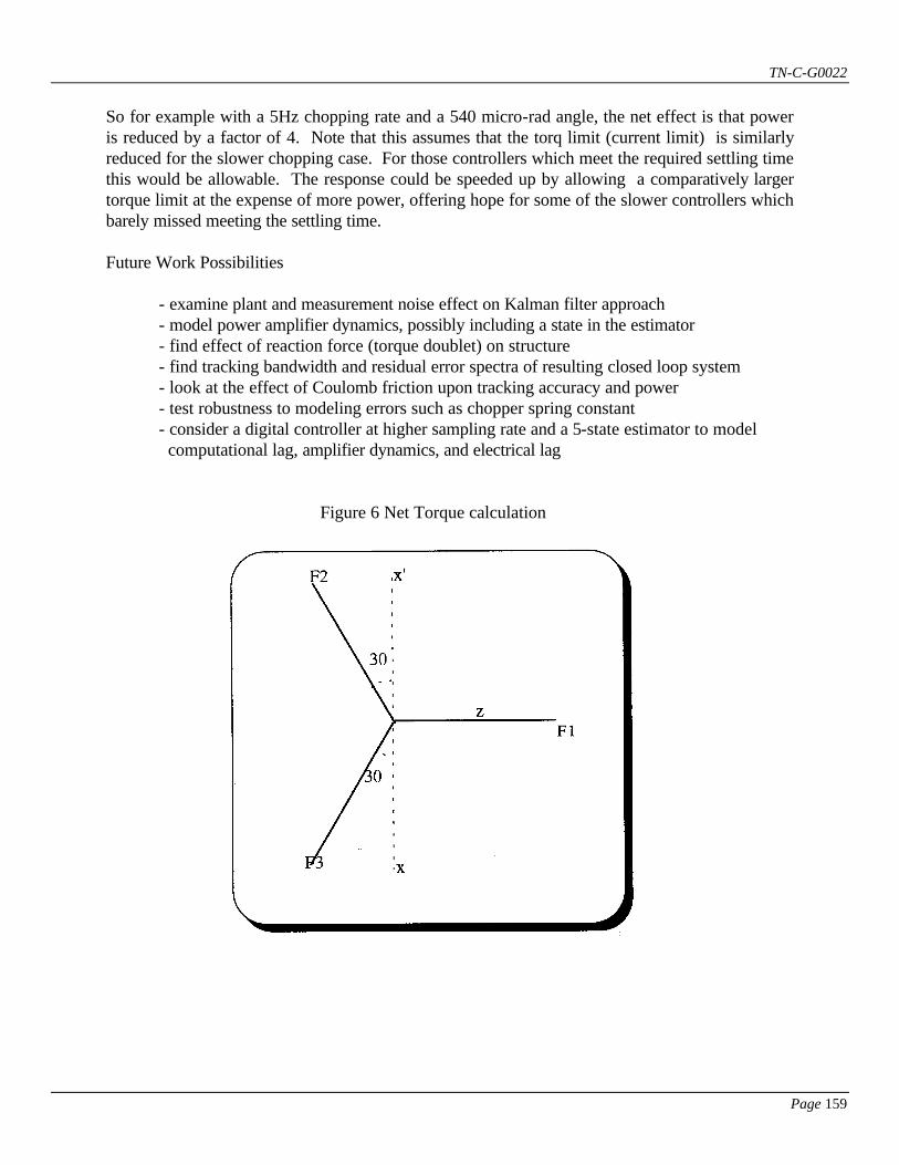
TN-C-G0022

Page 159

So for example with a 5Hz chopping rate and a 540 micro-rad angle, the net effect is that power is reduced by a factor of 4. Note that this assumes that the torq limit (current limit) is similarly reduced for the slower chopping case. For those controllers which meet the required settling time this would be allowable. The response could be speeded up by allowing a comparatively larger torque limit at the expense of more power, offering hope for some of the slower controllers which barely missed meeting the settling time. Future Work Possibilities - examine plant and measurement noise effect on Kalman filter approach - model power amplifier dynamics, possibly including a state in the estimator - find effect of reaction force (torque doublet) on structure - find tracking bandwidth and residual error spectra of resulting closed loop system - look at the effect of Coulomb friction upon tracking accuracy and power - test robustness to modeling errors such as chopper spring constant - consider a digital controller at higher sampling rate and a 5-state estimator to model computational lag, amplifier dynamics, and electrical lag

Figure 6 Net Torque calculation

TN-C-G0022

Page 160

Appendix A4 To: Rick McGonegal From: Mike Burns Date: April 28,1993 Subject: Image Smear Error Budget with Required Servo Bandwidth and Sampling Rate Introduction The value of an active optics system is that a more stable image may be obtained by tip-tilting the secondary mirror to remove random image motion. If the random motion of the image is relatively slow compared to the servo driving the secondary, then compensation will be good and the resulting image motion will be small. Summary The requirment for reducing image smear due to atmospheric effects may be met with a servo closed loop bandwidth of 15Hz sampled at 100Hz. The requirment for reducing image smear due to wind shake may be met with a servo closed loop bandwidth of 40Hz sampled at 200Hz. Problem The total image smear error budget is 0.03 arcsec. This represents an increase in the 50% encircled energy. For simulation purposes it is easier to consider the target to be a point and therefore the RMS motion of the image centroid is more relevant. It is believed that the relationship between 50% encircled energy and centroid motion is near 1:1.35, so the error budget for centroid motion is taken to be 0.022 arcsec RMS or approximately 0.108 micro-radians RMS per axis. The 0.108 micro-radian error budget is for wind-shake and other unmodelled disturbance torques. These torques are considered to be statistically independent so the net RMS level is obtained by RSS-ing (root sum squaring) all of the components. The target for wind shake is that it take up one quarter of the total image smear budget power or one half of the RMS, so the target wind shake after compensation is 0.054 micro-radians RMS. Atmospheric effects are considered separately from the image smear error budget with the requirement that the power in atmospheric noise be reduced by 90%. The uncompensated atmospheric image motion is calculated to be 0.96E-12 rad^2. Multiplying this by 0.1 and taking the square root gives the allowable compensated RMS of 0.31 micro-rad. After discussions with representatives of Starfire Labs, correlation noise will account for 0.083 micro-rad of the 0.31 micro-rad, which means that compensated atmospheric noise must be reduced to 0.3 micro-rad RMS.

TN-C-G0022

Page 161

The 0.08 micro-rad correlation noise is calculated assuming that lambda/R0 Enoise = ---------------- SNR where lambda= 2.2 microns R0 = 1.33 meters SNR = 20. Disturbance Torques The table below shows the expected RMS level of disturbance induced image motion both before and after compensation. Note that the requirement on atmospheric induced error is met for a 15Hz servo bandwidth operating at 100Hz sampling rate but that the requirement on windshake mandates a much higher bandwidth of 40Hz and sampling rate of 200Hz.

Table 1: List of Disturbance Torques Before and After Compensation

Disturbance Torque Uncompensated RMS

(micro-radians)

Compensated with BW=15Hz,rate=100Hz

(micro-radians)

Compensated with BW=40Hz,rate=200Hz

(micro-radians) Atmospheric 0.98 0.25 0.11 Wind shake (Tz) 0.85 0.23 0.10 Other unmodelled 0.17 0.06 0.04 The unmodelled disturbance torques include bearing friction, servo torque ripple and servo reaction torques transmitted through the telescope structure. The compensated values above assume that the disturbances have a bandwidth of 1Hz. If the actual bandwidth is less, then filtering action will improve and a larger uncompensated RMS level will be tolerable. The tradeoffs are shown below in the results section. Figures 1,2 and 3 show the power spectra for atmospheric induced errors before compensation, after compensation with 15Hz bandwidth and after compensation with 40Hz bandwidth. The uncompensated power spectrum is a modified Greenwood distribution which falls off like the 2/3rds power of frequency up to a certain cutoff then falls off like the 11/3rds power afterwards. This distribution is possibly overly conservative, and more accurate data is expected from Starfire Labs soon. If the atmospheric data used for this report were overly conservative then the new data would require less bandwidth and slower sampling than the 15Hz and 100Hz quoted here. The spectra for wind shake in the z-direction, Tz, before and after the same compensation are shown in figures 4, 5 and 6. The corresponding spectra for Tx are expected to be the same for an orthogonal wind. The example spectra for unmodelled disturbance torques are in figures 7, 8, and 9. The unmodelled disturbance torques are modeled as first order Markov processes, that is

TN-C-G0022

Page 162

what noise through a low pass filter with a single pole. Results would improve slightly for higher order models of a given bandwidth and RMS because the fraction of power at higher frequencies would be smaller. All spectra are double-sided, meaning that it is necessary to integrate from negative infinity to positive infinity frequency to encompass all of the energy. Tip/tilt Model Figure 10 shows the block diagram representation of the single axis model of the secondary tip/tilt system used for this study. The input at the left, theta_c is assumed to be a random process with some known spectrum representing uncompensated image motion. The variable theta_o represents the actual position of the secondary and the difference between theta_c and theta_o is the error after compensation which is desired to be near zero. The error signal passes through a sample and hold to give the measured error theta_m. The sample and hold allows the analog model of the servo to interact with the digital control system and causes a small amount of degradation. The measured error is fed to the servo model which acts to attempt to drive the error to zero. The servo model block is theta_o(s) w0*w0 ------------ = ------------ theta_m(s) s^2 + s*2*w0 where w0=2*pi*BW with BW being the desired closed loop bandwidth. Good design dictates that sampling rate should be 5-20 times the closed loop bandwidth. It is noticed that for a bandwidth of 15 Hz and a sample rate of 100Hz the closed loop has a phase margin of 76 degrees. The signal processing delay of 500 microseconds has been neglected in the model because it is small. This delay gives 2.7 degrees of phase lag at 15Hz, which will put the phase margin at 73 degrees, still above our target of 70 degrees. Figure 11 shows the squared magnitude of the filter function from theta_c to theta_e for a 15Hz bandwidth servo loop and 100Hz sampling. The compensated error spectrum (e.g. fig. 2) is found by multiplying this curve point by point times the input spectrum (e.g. fig. 1). The compensated error spectrum is then integrated over frequency to give compensated power and then taking the square root gives compensated RMS. Note that both uncompensated atmospheric (fig. 1) and uncompensated windshake (fig. 4) start to fall off around 2.5 Hz. At this frequency the squared filter function is around 0.1, which attenuates the input power by a factor of 10. Another interesting point to notice about figure 11 is the overshoot magnitude of 1.3 near 18Hz. The filter not only fails to attenuate input power at this frequency but actually amplifies it. The overshoot is undesirable but is an inevitable part of having 70 degrees of phase margin. Increasing the sampling rate for a given servo bandwidth will improve the phase margin and shrink the overshoot.

TN-C-G0022

Page 163

Results The following table shows the resulting image motion after compensation for a range of servo bandwidths. The sampling rates for each bandwidth are also shown. The "compensated other disturbance" values shown are chosen such that for the z-axis the RSS of Tz and the "other" is equal to the total error budget of 0.2 micro-rad.

Table 2: RMS Image Motion After Compensation for Various Disturbance Torques

Servo BW

(Hz)

Sample Rate

(Hz)

Compensated Atmospheric (micro-rad)

Compensated Windshake Tz

(micro-rad)

Compensated other distrb (micro-rad)

5 100 0.54 0.53 ----- 7 100 0.44 0.43 ----- 10 100 0.34 0.32 ----- 15 100 0.25 0.23 ----- 20 100 0.20 0.18 ----- 25 200 0.16 0.15 ----- 30 200 0.14 0.13 ----- 35 200 0.12 0.11 ----- 40 200 0.11 0.10 0.04

Table 3 below shows the effect of the disturbance toorque bandwidth on the servo loop's capability to reject it.

Table 3: Allowable Uncompensated Other Disturbance Torques

Servo BW

(Hz)

Sample Rate

(Hz)

Compensated other distrb (micro-rad)

Uncomp at 0.1 Hz BW (micro-rad)

Uncomp at 1.0 Hz BW (micro-rad)

Uncomp at 10.0 HzBW

(micro-rad) 40 200 0.04 0.53 0.17 0.07

Note that as the bandwidth of the disturbance torque approaches the bandwidth of the servo loop, for example the 40 Hz servo and 10Hz disturbance, the servo loop is capable of removing only a small amount of the disturbance power and the compensated RMS (0.04 micro-rad) approaches the uncompensated RMS (0.07 micro-rad). Alternately, if the servo loop is very fast compared to the disturbance torque, then the uncompensated RMS (0.53) is attenuated greatly to give the compensated RMS (0.04). This is a savings of factor 13 in RMS or 178 in power. If the unmodelled disturbance torques have bandwidth in excess of 10Hz, there is very little savings to be had in compensation so they must be kept small. Conclusion Reduction of atmospheric induced image smear turns out to be an easier task than reduction of the windshake induced image smear. It is easier in the sense of requiring lower servo bandwidth and corresponding lower sampling rate: 15Hz bandwidth and 100Hz sampling vs. 40Hz

TN-C-G0022

Page 164

bandwidth and 200Hz sampling. The reason for this difference is partly that windshake has proportionally more of its energy at higher frequencies and partly that the requirements are different. It is required to reduce atmospheric noise by 90% in power which corresponds to a factor of 0.31 in RMS. The windshake must be reduced from 0.85 microrad RMS to 0.1 microrad RMS, a factor of 0.12 in RMS. List of Figures Figure 1 Greenwood Atmospheric Error Before Compensation Figure 2 Greenwood Atmospheric Error After 15Hz Compensation Figure 3 Greenwood Atmospheric Error After 40Hz Compensation Figure 4 Wind Shake in Z-Direction Before Compensation Figure 5 Wind Shake in Z-Direction After 15Hz Compensation Figure 6 Wind Shake in Z-Direction After 40Hz Compensation Figure 7 Other Disturbance Before Compensation Figure 8 Other Disturbance After 15Hz Compensation Figure 9 Other Disturbance After 40Hz Compensation Figure 10 Simulation Block Diagram Figure 11 Example Filter Attenuation for 15Hz Bandwidth

TN-C-G0022

Page 165

Appendix A5 To: Rick McGonegal From: Mike Burns Re: Comparison of Gemini Tip-Tilt Atmospheric Correction Simulation Results to

those of the FTAS Project Ref: Report on the Fast Two-Axis Secondary Project, Stephen T. Ridgeway This is meant as a brief comparison between my results and those obtained by the prototype project on the 2.1m telescope at Kitt Peak.

Criterion for Comparison FTAS Project My Simulation Input RMS of Atmospheric Distirbance

x-axis: 1.6 microrad y-axis: 0.93 microrad They believe that x-acxis is needlessly large due to a mechanical resonance.

0.98 microrad

Quality of Atmospheric Disturbance

Falls off like f^(-2/3) to 80Hz Falls off like f^(-2/3) to 2.5Hz Falls off like f^(-11/3) after 100Hz

Required Sample Rate for Removing 90% Power

200Hz 100Hz Consistent with lower high-frequency noise

Signal Processing Delay 1 ZOH for Digitization 1 ZOH for Centroider

1 ZOH for Digitization Centroider Neglected

Compensation for Delay lead-lag compensator Not deemed necessary for this model. Lead-lag applied for longer delay case studied earlier.

Servo Bandwidth 10 Hz (measured at 3db point) 6Hz (measured at 3db point) 15Hz pole position

Servo Nature 3 poles 2 poles; Will not fall off as fast as 3 poles, thus will not reject noise as well, but is also less sensitive to modeling errors and loop delay.

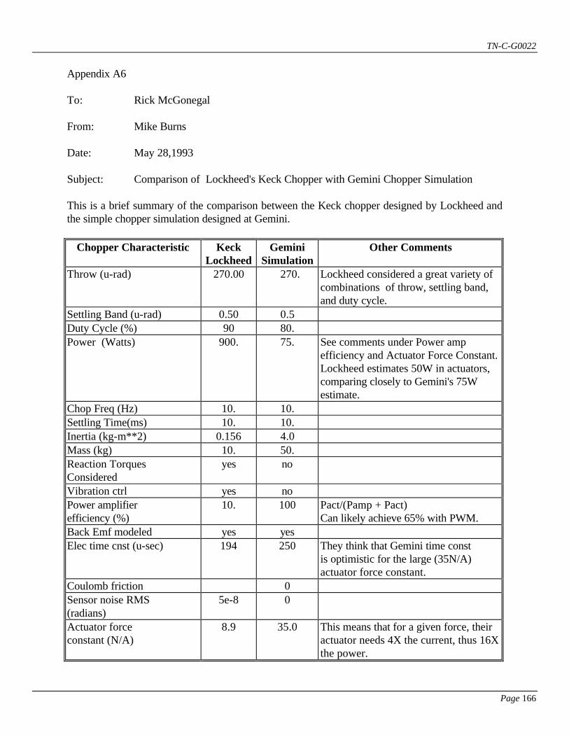
TN-C-G0022

Page 166

Appendix A6 To: Rick McGonegal From: Mike Burns Date: May 28,1993 Subject: Comparison of Lockheed's Keck Chopper with Gemini Chopper Simulation This is a brief summary of the comparison between the Keck chopper designed by Lockheed and the simple chopper simulation designed at Gemini.

Chopper Characteristic Keck Lockheed

Gemini Simulation

Other Comments

Throw (u-rad) 270.00 270. Lockheed considered a great variety of combinations of throw, settling band, and duty cycle.

Settling Band (u-rad) 0.50 0.5 Duty Cycle (%) 90 80. Power (Watts) 900.

75. See comments under Power amp

efficiency and Actuator Force Constant. Lockheed estimates 50W in actuators, comparing closely to Gemini's 75W estimate.

Chop Freq (Hz) 10. 10. Settling Time(ms) 10. 10. Inertia (kg-m**2) 0.156 4.0 Mass (kg) 10. 50. Reaction Torques Considered

yes no

Vibration ctrl yes no Power amplifier efficiency (%)

10. 100 Pact/(Pamp + Pact) Can likely achieve 65% with PWM.

Back Emf modeled yes yes Elec time cnst (u-sec) 194 250 They think that Gemini time const

is optimistic for the large (35N/A) actuator force constant.

Coulomb friction 0 Sensor noise RMS (radians)

5e-8 0

Actuator force constant (N/A)

8.9 35.0 This means that for a given force, their actuator needs 4X the current, thus 16X the power.

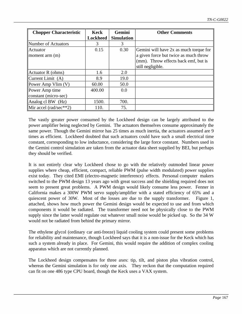
TN-C-G0022

Page 167

Chopper Characteristic Keck Lockheed

Gemini Simulation

Other Comments

Number of Actuators 3 3 Actuator moment arm (m)

0.15 0.30 Gemini will have 2x as much torque for a given force but twice as much throw (mm). Throw effects back emf, but is still negligible.

Actuator R (ohms) 1.6 2.0 Current Limit (A) 8.9 19.0 Power Amp Vlim (V) 60.00 50.0 Power Amp time constant (micro-sec)

400.00 0.0

Analog cl BW (Hz) 1500. 700. Mir accel (rad/sec**2) 110. 75. The vastly greater power consumed by the Lockheed design can be largely attributed to the power amplifier being neglected by Gemini. The actuators themselves consume approximately the same power. Though the Gemini mirror has 25 times as much inertia, the actuators assumed are 9 times as efficient. Lockheed doubted that such actuators could have such a small electrical time constant, corresponding to low inductance, considering the large force constant. Numbers used in the Gemini control simulation are taken from the actuator data sheet supplied by BEI, but perhaps they should be verified. It is not entirely clear why Lockheed chose to go with the relatively outmoded linear power supplies where cheap, efficient, compact, reliable PWM (pulse width modulated) power supplies exist today. They cited EMI (electro-magnetic interference) effects. Personal computer makers switched to the PWM design 13 years ago with great success and the shielding required does not seem to present great problems. A PWM design would likely consume less power. Fenner in California makes a 300W PWM servo supply/amplifier with a stated efficiency of 65% and a quiescent power of 30W. Most of the losses are due to the supply transformer. Figure 1, attached, shows how much power the Gemini design would be expected to use and from which components it would be radiated. The transformer need not be physically close to the PWM supply since the latter would regulate out whatever small noise would be picked up. So the 34 W would not be radiated from behind the primary mirror. The ethylene glycol (ordinary car anti-freeze) liquid cooling system could present some problems for reliability and maintenance, though Lockheed says that it is a non-issue for the Keck which has such a system already in place. For Gemini, this would require the addition of complex cooling apparatus which are not currently planned. The Lockheed design compensates for three axes: tip, tilt, and piston plus vibration control, whereas the Gemini simulation is for only one axis. They reckon that the computation required can fit on one 486 type CPU board, though the Keck uses a VAX system.

TN-C-G0022

Page 168

Another important difference not brought out in the table above is the underlying control strategy. The Gemini design makes a fast linear control loop which attempts to null the error difference between commanded chop angle and achieved. The Lockheed design is very clever in that it effectively generates a Fourier series of different frequency (or sequency) components to feed into the mirror control, thus taking advantage of the repetitive nature of the chopping waveform. The magnitude and phase of the different sequency components are computed adaptively, and it appears to take approximately 15 seconds for it to adapt. The Lockheed approach is not applicable to fast tracking, but it seems to hold promise for chopping.

TN-C-G0022

Page 169

Appendix A7 To: Rick McGonegal From: Mike Burns Date: June 9,1993 Subject: Effect of Filtering on Tracking Errors Reference: Open Loop Tracking, Rick McGonegal, April 22, 1993. Introduction A look up table (LUT) provides some improvement over the error associated with raw tracking. A digital filter with 40Hz bandwidth and 200Hz sampling provides more improvement. Summary With realistic noise (sinc-squared function) the RMS error may be reduced from 0.63 to 0.17 micro-radians by way of a 40Hz sampled-data servo system as shown in the table below.

Type of Noise Used RMS net before filtering (micro-rad)

RMS net after filtering (micro-rad)

Square corner at 20Hz 0.70 0.27 Sinc-squared function 0.63 0.17 none (only Look Up Table) 0.54 0.01 Derivation Figure 1 shows the block diagram used for the Matlab simulation of Appendix A. The spectral density out of the Raw-Tracking block, Phi1 is shown in Figure 2. The effective filtering of the LUT, Figure 3, provides some attenuation of the lower frequencies resulting in the power spectral density Phi2 of Figure 4. The noise associated with sampling the LUT, labeled Phi3 was modeled in the reference as having a square corner at 20Hz but is more realistically a sinc^2 function labeled Phi3 and plotted in Figure 5. Appendix B shows the derivation of the noise PSD. Figure 6 shows Phi4, Phi5 and the servo filter function, where Phi4 is the sum of power spectral densities before filtering, and Phi5 is the same after filtering.

TN-C-G0022

Page 170

Appendix B : Showing Noise PSD = (sig^2/fs) * sinc^2(pi * f/fs) Consider a sampled signal which has random errors x(t) which are uncorellated from sample to sample , and let the RMS of the error be denoted as sig. Note that this analysis nowhere assumes that the errors are Gaussian, although if they are then the RMS will equal to the standard deviation. It is desired to calculated to power spectral density of the noise in units^2/Hz, in this case rad^2/Hz. Clearly the mean and variance of the error are E[x] = 0 E[x^2]=sig^2 . The autocorrelation is defined as psi(t) = E[x(t1)*x(t1+t)]. For this case, it may be shown that psi(t) = 0 for |t|>ts = sig^2 * |1-t/ts| for |t|<ts The fact that the autocorrelation is zero for times greater than the sampling period is a direct result of different pulses having no correlation. Note that the second line of the autocorrelation above degenerates to sig^2 when t=0, which is to say that the correlation of a pulse with itself is the sig^2. For t between these extremes the autocorrelation falls off linearly to represent the proportion of a pulse which overlaps with itself when doing the correlation. The power spectral density as a function of radian frequency is related to the autocorrelation by the Fourier transform Phi(w) = psi(t) * exp(-jwt) dt Since psi(t) is an even function due to the absolute value, the imaginary (i.e. sin(wt)) part of the above integrates to zero. The real part (i.e. cos(wt)) can be integrated from 0 to ts and doubled: Phi(w) = 2*sig^2 (1 - t/ts)*cos(wt) dt t=ts Phi(w) = 2*sig^2 [ sin(wt) - 1*(cos(wt) + t*sin(wt) ) ] -------- - ------- --- w ts w^2 w t=0

TN-C-G0022

Page 171

Phi(w) = 2*sig^2 [ 1 - cos(w*ts)] ---------- ts*w^2 Using the trig identity that [1-cos(u)] = 2*sin^2(u) this becomes Phi(w) = 4*sig^2*sin^2(w*ts) --------- ts*w^2 Phi(w) = sig^2*ts*sin^2(w*ts/2) ---------- (w*ts/2)^2 Phi(w) = sig^2*ts*sinc^2(w*ts/2) Substituting w=2*pi*f and fs=1/ts gives Phi(w)=sig^2*ts*sinc^2(pi*f/fs) QED. It's worth noting that this is also a justification for the frequently used Phi=sig^2*ts to use as the spectral density of white noise represented by a sampled data system, since the sinc function is very flat and equal to 1 in the vicinity of zero, that is when f<<fs. A digital system usually includes filtering well below the sampling rate, so the roll off in the sinc function near fs goes unnoticed and the white noise approximation holds.

TN-C-G0022

Page 172

Appendix A8 To: Rick McGonegal From: Mike Burns Date: August 23,1993 Subject: Restriction Imposed on Tip-tilt for an Off-Axis Guide Star Reference [1] Private Correspondence between R. McGonegal and R. Racine August 20, 1993. Introduction If one attempts to do tip-tilt compensation on a science object by tracking a bright nearby object, what will be the effect of the angular difference between the two? Summary Unless an error has been made in calculating the results of this technical note, it is not practical to do off-axis atmospheric tip-tilt correction if 90% sky coverage is desired near the North Galactic Pole. It is assumed that % reduction in tip-tilt power is used as a measure of practicality. This may show that % reduction in tip-tilt power is not a good measure of improvement in the image. Starfire Lab's results show larger radii with significant Strehl improvement. Calculations There will be an error introduced in doing tip-tilt correction on one object but looking at a different nearby object. The requirement for the Gemini project is that the total atmospheric tip-tilt must be reduced in power to 10% of the uncompensated value. From [1] the variance of error introduced by using an off-axis guide star is sig_iso^2 = (x/r)^2 * sig_unc^2 where sig_unc is the uncompensated RMS, r is the correlation radius (arcminutes), and x is the angular difference (arcminutes) between guide star and science object. The table below shows the normalized variance, that is by what factor the error power is attenuated when the difference between the guide star and science object is specified:

normalized Diameter if normalized Effective Req'd number Required

TN-C-G0022

Page 173

distance (guide-science)

= x/r

isokinetic diam=3.4 arcmin

tip-tilt power TTN= (x/r)^2

tip-tilt pwr reduction

TTPR

of stars per square arcmin

for 90% N

Visual Magnitude for 90% V

0.00 0.00 0.00 0.90 inf inf 0.10 0.34 0.01 0.90 25.30 32.20 0.20 0.64 0.04 0.89 6.30 28.40 0.30 1.02 0.09 0.87 2.80 26.10 0.40 1.36 0.16 0.81 1.60 24.60 0.50 1.70 0.25 0.73 1.00 23.30 0.60 2.04 0.36 0.63 0.70 22.20 0.70 2.38 0.49 0.50 0.52 21.50 0.80 2.72 0.64 0.35 0.40 20.70 0.90 3.06 0.81 0.18 0.31 20.10 1.00 3.40 1.00 -0.01 0.25 19.50 inf inf n/a n/a 0.00 -inf

To get a factor of 2 reduction in tip-tilt power requires a guide star within 0.7 correlation lengths, which in turn requires that stars to magnitude 21.5 be used. In the above table, the effective tip-tilt power reduction represents how much of the noise is removed from the science object. If it is assumed that the guide star has 90% of its power removed, then the remaining noise is the root sum square of 0.1 and the normalized power of column 2. Thus the effective tip-tilt power reduction (TTPR) will be given by TTPR = 1 - sqrt ( 0.1^2 + TTN^2). Ideally, TTPR will be unity, representing all tip-tilt power removed from the science object. This is not possible though because of the assumed 0.1 residual power in the guide star, so the best practical TTPR=0.9. As the angular difference between the guide star and science object increases, the TTPR will shrink and eventually become negative, denoting that the process is actually adding noise to the science object. The correlation radius (isokinetic radius) is empirically given by 0.3*Dtel 0.3* 8 r = ---------- = --------- = 4.8e-4 rad = 1.7 arcmin hturb 5000 where Dtel = the telescope diameter and hturb is the turbulence height. In order to have a 90% probability of finding a star within a given diameter D_90 requires N stars per square arcminute. D_90 = 1.211/sqrt(0.5*N) thus

TN-C-G0022

Page 174

N = 2*(1.211/2x)^2 The number of stars per square arcminute with visual magnitude <V at the North Galactic Pole is log10(N) = 0.158*V - 3.68 3.68 + log10(N) V = ------------------ 0.158 The above table has some interesting implications. At zero difference between the science object and the guide star, there is no noise introduced. This should be expected since it is assumed that the guide star is being tracked exactly. At the other end of the scale, things degrade badly. In fact, if the distance is great, noise is in fact amplified by 2. So when the science object is not near the guide star, we would do better to suffer with the noise as it is, rather than use a guide star. The mathematical break-even point seems to be at x/r = 1.0. It should be noted that the quadratic approximation to correlation is only for small off-axis distances. At x/r=infinity, one would expect the normalized tip-tilt power TTN=2 because science object and guide star will have no correlation. Clearly the quadratic approximation breaks down before x/r=sqrt(2) but is expected to be acceptable at unity.

TN-C-G0022

Page 175

Appendix A9 To: Rick McGonegal From: Mike Burns Date: August 23,1993 Subject: SNR vs. Sample Rate for Tip-Tilt Using an Off-Axis Guide Star Reference [1] Burns, Mike "Restriction Imposed on Tip-tilt for an Off-Axis Guide Star" Technical Note Gemini 8-M Telescopes Project, August 1993. Introduction It is desired to use a bright guide star to attempt to decorrellate atmospheric noise in a faint science object. A larger field of view is more likely to have a brighter guide star which will in turn have a correspondingly better SNR (signal/noise ratio). Slower sampling will collect more photons, which will also improve SNR. This note shows the relationship between sampling rate and SNR for three different effective fields of view. Summary The SNR for a 3.5 arcminute field sampled at 200Hz is nearly 10. Calculations The science field is known to be 3.5 arcminutes in diameter and the guide field is 8.0 arcminutes in diameter. The area of the annulus obtained by removing the science field and leaving the guide field is equivalent to a circle of diameter 7.2 arcminutes ( = sqrt(8.0^2 - 3.5^2) ). From reference [1] it appears that the maximum diameter at which the atmospheric tip-tilt is reduced by a factor of two is 2.4 arcminutes. These three diameters are considered below and are marked on the attached figure. Given a diameter D_90 in arcminutes, if it is desired that there be a 90% chance of finding a sufficiently bright star, then the number of stars required per square arcminute is: N = 2*(1.211/D_90)^2 . N(2.4) = 0.52 N(3.5) = 0.24 N(7.2 )= 0.057

TN-C-G0022

Page 176

Empirically it is known that the number of stars per square arcminute near the North Galactic Pole is related to the visual magnitude V such that V = (3.68 + log10(N)) / 0.158 , V(2.4) = 21.5 V(3.5) = 19.4 V(7.2) = 15.4 and flux (electrons/ sec) is flux = 1.1e12 / ( 10 ^ (V/2.5) ). flux(2.4) = 2.8e3 flux(3.5) = 1.9e4 flux(7.2) = 7.6e5 So from a given diameter D_90, we can compute the flux as above. SNR is related to flux and sampling rate (fs) by SNR = sqrt ( flux/ fs). SNR(D_99=2.4, fs=200Hz) = 3.7 SNR(D_99=3.5, fs=200Hz) = 9.7 SNR(D_99=7.2, fs=200Hz) = 61.6 The sample rate of 200Hz is chosen arbitrarily to show the example SNR's above for the various diameters. The attached figure shows SNR plotted vs. sampling rate for the three effective diameters, 2.4, 3.5 and 7.2 arcminutes, representing a minimum diameter, the science field, and the annulus surrounding the science field.

TN-C-G0022

Page 177

Appendis A10 GEMINI 8-METRE TELESCOPES PROJECT

CONTROLS GROUP _____________________________________________________________________________ To: File Copied To : R. McGonegal From: Mike Burns Date: November 18, 1993 Subject: Some Tracking Error Results for the Nonlinear Baseline Telescope Simulation The accompanying table summarizes the performance of the baseline nonlinear simulation for different levels of friction, angular measurement quantization and tracking rate. The parameters are varied by orders of magnitude from their nominal values in order to note the effect on overall tracking accuracy. The three columns of the table represent the three axes being commanded: altitude, azimuth and cassegrain. Since the telescope model was derived for zenith pointing, only the altitude command directly affects tracking errors. The azimuth and cassegrain commands only affect the tracking error indirectly by way of cross coupling between the axes. The RMS tracking errors shown in the table would likely be orders of magnitude greater for the azimuth and cassegrain axes with non-zenith pointing. The altitude axis seemed relatively immune to the effect of increasing or decreasing bearing friction. The azimuth axis became unstable when friction was increased by 10 times and the cassegrain became unstable at 100 times nominal friction. There is some debate about what the nominal level of bearing friction should be. The values used for this study were recommended by Kaman Aerospace in their fax dated 8/17/93 and might be overly conservative by a factor of 10. This issue is being investigated. Angular quantization size affected RMS tracking for the altitude axis to a roughly square root relation, while the azimuth axis saw a slightly faster increase at roughly a 0.7 power. The cassegrain axis was nearly immune to quantization level, but of course it is likely to suffer considerably for non-zenith pointing. When tracking rate was increased from the nominal sidereal rate (73 micro-rad/sec), the altitude axis tracking error increased by the square root, but showed little improvement for very slow tracking rates. The azimuth axis showed small improvements for slower tracking rates as did the cassegrain. One test case was run corresponding to the high azimuthal rates seen within 0.5 degrees of zenith. The altitude command was set at 15 arcsec/sec, the azimuth at 0.5 deg/sec and the cassegrain at -

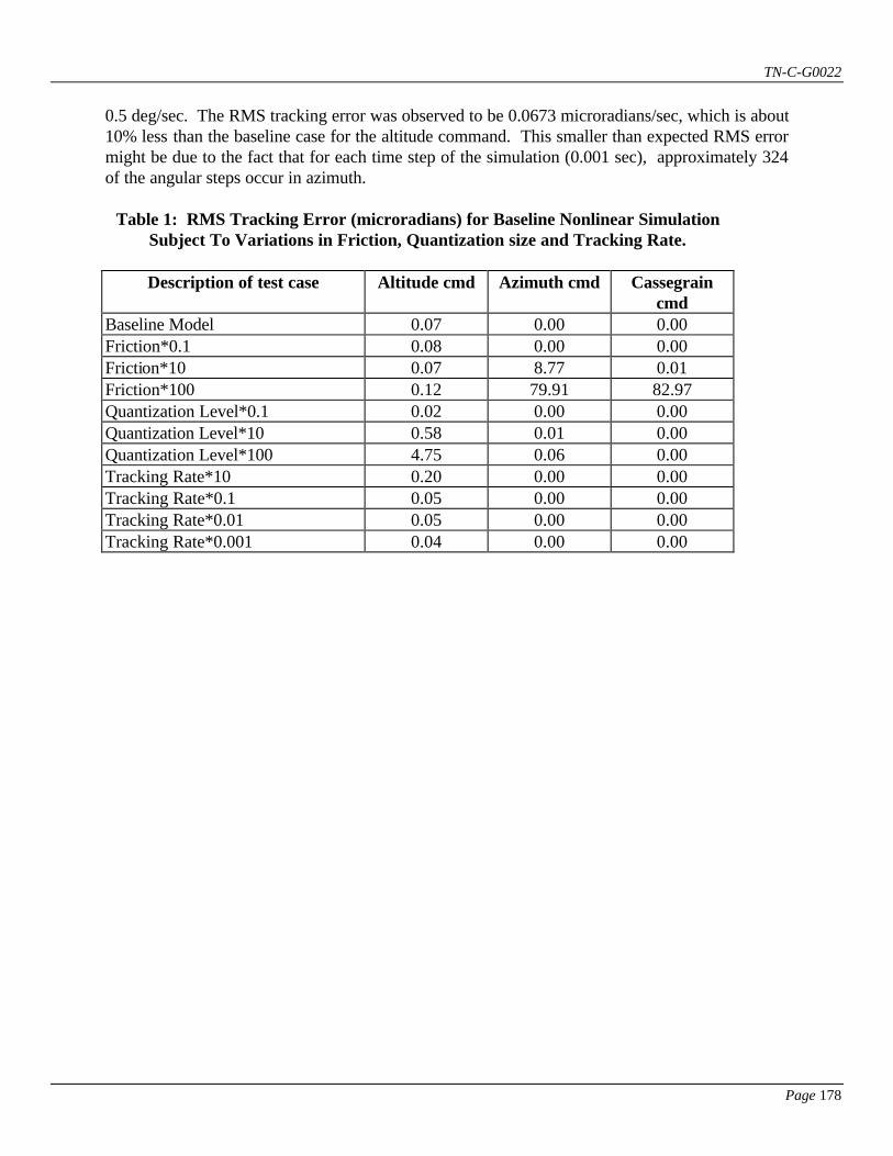
TN-C-G0022

Page 178

0.5 deg/sec. The RMS tracking error was observed to be 0.0673 microradians/sec, which is about 10% less than the baseline case for the altitude command. This smaller than expected RMS error might be due to the fact that for each time step of the simulation (0.001 sec), approximately 324 of the angular steps occur in azimuth.

Table 1: RMS Tracking Error (microradians) for Baseline Nonlinear Simulation Subject To Variations in Friction, Quantization size and Tracking Rate.

Description of test case

Altitude cmd Azimuth cmd Cassegrain

cmd Baseline Model 0.07 0.00 0.00 Friction*0.1 0.08 0.00 0.00 Friction*10 0.07 8.77 0.01 Friction*100 0.12 79.91 82.97 Quantization Level*0.1 0.02 0.00 0.00 Quantization Level*10 0.58 0.01 0.00 Quantization Level*100 4.75 0.06 0.00 Tracking Rate*10 0.20 0.00 0.00 Tracking Rate*0.1 0.05 0.00 0.00 Tracking Rate*0.01 0.05 0.00 0.00 Tracking Rate*0.001 0.04 0.00 0.00

TN-C-G0022

Page 179


CONTROLS GROUP _____________________________________________________________________________ To: File Copied To : R. McGonegal From: Mike Burns Date: December 7, 1993 Subject: Updated Tracking Error Results for the Nonlinear Baseline Telescope Simulation The accompanying tables summarizes the performance of the baseline nonlinear simulation for different levels of friction, angular measurement quantization and tracking rate. The parameters are varied by orders of magnitude from their nominal values in order to note the effect on overall tracking accuracy. The first table shows tracking errors in microradians for tiptilt off and the second table is for tiptilt on. The four columns of data per table represent four cases of tracking commands. The first represents an altitude command equal to sidereal rate (15 arcsec/sec = 7.3e-5 rad/sec) with azimuth and cassegrain fixed. The second column is for azimuth command at sidereal rate, and the other two axes are fixed. The third column is for cassegrain command at sidereal rate. The fourth column represents a case near the zenith where altitude is moving at sidereal rate, azimuth is moving at 0.5deg/sec and cassegrain is moving at -0.5deg/sec. The bearing friction used in this study corresponds to the corrected values obtained from Kaman as of 12/3/93. These values of coulomb friction and stiction are one tenth of the values used previously, due to an error in the decimal place reported by Kaman. The linear component of friction remains unchanged from the earlier studies. Mark Warner believes that the updated values of bearing friction might still be too large. Table 2 shows the RMS errors for tiptilt turned on. The benign case shows 0.017 microradians for all 4 commanded inputs due to the centroid measurment noise. Performance is worse for tiptilt on (Table 2) than when tiptilt is turned off (Table 1) because an intentionally conservative and pathological case was chosen. The guide star is modelled as being 6 arcminutes from the axis of rotation and at an angle of 45 degrees from the horizontal (TX) axis. The science object is modelled as being 1.7 arcminutes from the axis of rotation at an angle of -135 degrees from the horizontal axis. That is, the science object is on the opposite side of the axis of rotation from the guide object. This causes tiptilt to accentuate any errors in rotation about the axis of the field of view, such as those errors caused by the cassegrain rotator. Errors which tend to translate the entire field, such as those associated with the altitude drive, will be corrected.

TN-C-G0022

Page 180

In Table 2, with tiptilt on, the case of having an azimuth command seems to be troubled by friction. In order to meet the desired spec of 0.07 microrad after compensation, friction must be reduced by approximately a factor of 3 for the azimuth axis. For the case of a sidereal command for the cassegrain rotator, it seems that the quantization must be improved by a factor of 5 for the cassegrain axis. The same conclusion can be drawn for the case of near-zenith pointing. Table 1: RMS Tracking Error (microradians) for Baseline Nonlinear Simulation

With Tiptilt Off Subject To Parameter Variations

Description of test case

Altitude cmd

Azimuth cmd

Cassegrain cmd

Near- Zenith

Benign Case 0.00 0.00 0.00 0.01 Baseline Model 0.06 0.04 0.07 0.11 Friction*0.1 0.05 0.01 0.04 0.01 Friction*10 0.16 1.16 2.50 0.11 Friction*100 6.61 15.50 17.20 0.46 Quantization Level*0.1 0.00 0.06 0.01 0.05 Quantization Level*10 0.41 0.09 0.65 0.51 Quantization Level*100 4.74 0.09 11.63 3.90 Tracking Rate*10 0.04 0.19 0.07 0.22 Tracking Rate*0.1 0.04 0.02 0.11 0.07 Tracking Rate*0.01 0.05 0.00 0.13 0.07 Tracking Rate*0.001 0.04 0.00 0.19 0.13 Table 2: RMS Tracking Error (microradians) for Baseline Nonlinear Simulation

With Tiptilt On Subject to Parameter Variations

Description of test case Altitude cmd

Azimuth cmd

Cassegrain cmd

Near- Zenith

Benign Case 0.02 0.02 0.02 0.02 Baseline Model 0.02 0.19 0.26 0.27 Friction*0.1 0.02 0.02 0.15 0.27 Friction*10 5.00 5.09 2.65 0.27 Friction*100 30.24 29.16 38.96 2.15 Quantization*0.1 0.02 0.19 0.03 0.03 Quantization*10 0.02 0.35 2.76 2.13 Quantization*100 0.14 0.45 51.49 17.19 Tracking Rate*10 0.02 0.71 0.20 0.27 Tracking Rate*0.1 0.02 0.03 0.46 0.21 Tracking Rate*0.01 0.02 0.02 0.55 0.21 Tracking Rate*0.001 0.02 0.03 0.86 0.52

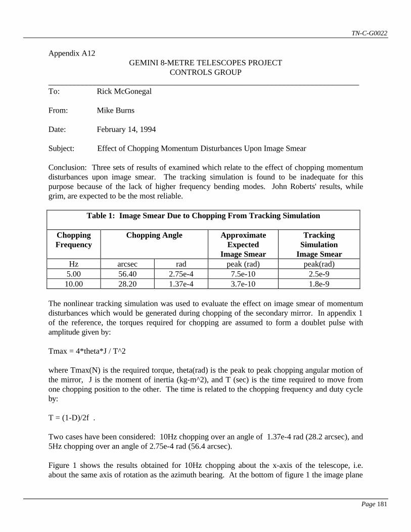
TN-C-G0022

Page 181


CONTROLS GROUP _____________________________________________________________________________ To: Rick McGonegal From: Mike Burns Date: February 14, 1994 Subject: Effect of Chopping Momentum Disturbances Upon Image Smear Conclusion: Three sets of results of examined which relate to the effect of chopping momentum disturbances upon image smear. The tracking simulation is found to be inadequate for this purpose because of the lack of higher frequency bending modes. John Roberts' results, while grim, are expected to be the most reliable.

Table 1: Image Smear Due to Chopping From Tracking Simulation

Chopping Frequency

Chopping Angle

Approximate Expected

Image Smear

Tracking Simulation

Image Smear Hz arcsec rad peak (rad) peak(rad)

5.00 56.40 2.75e-4 7.5e-10 2.5e-9 10.00 28.20 1.37e-4 3.7e-10 1.8e-9

The nonlinear tracking simulation was used to evaluate the effect on image smear of momentum disturbances which would be generated during chopping of the secondary mirror. In appendix 1 of the reference, the torques required for chopping are assumed to form a doublet pulse with amplitude given by: Tmax = 4*theta*J / T^2 where Tmax(N) is the required torque, theta(rad) is the peak to peak chopping angular motion of the mirror, J is the moment of inertia (kg-m^2), and T (sec) is the time required to move from one chopping position to the other. The time is related to the chopping frequency and duty cycle by: T = (1-D)/2f . Two cases have been considered: 10Hz chopping over an angle of 1.37e-4 rad (28.2 arcsec), and 5Hz chopping over an angle of 2.75e-4 rad (56.4 arcsec). Figure 1 shows the results obtained for 10Hz chopping about the x-axis of the telescope, i.e. about the same axis of rotation as the azimuth bearing. At the bottom of figure 1 the image plane

TN-C-G0022

Page 182

motions in the x and y directions are shown. As expected the y image plane motion is far larger, equal to approximately 1.2e-9 rad. This is relatively small compared to the error budge of 1.7e-8 rad. The upper right plot of figure 1 shows the chopping torques over a short time interval and the upper left plot shows the motions reflected back into the secondary mirror. Figure 2 shows that for the same 10Hz chopping about the y-axis (orthogonal to the altitude axis), the response is predominantly in the x image direction. The magnitude is approximately 1.8e-9 rad. Figure 3 shows the effect of 5Hz chopping about the y-axis. Even though the primary mirror is moving twice as far as for the 10Hz case, the image smear increases only 30% to 2.5e-9 rad, which is still small compared to the error budget of 1.7e-8. A quick back of the envelope calculation can give the expected image plane motion for chopping. Consider a force reacting against 2 free bodies having different masses. Then the motion of each body will be inversely proportional to the respective mass or inertia. The inertias of the mirror and telescope tube section are in ratio by roughly 1e6. J(mirror) = 4 kg-m^2 J(telescope) = 3e6 kg-m^2 The motion of the secondary mirror is given as theta, so the amplitude of the motion expected by the telescope is theta(telescope) = theta(mirror) * J(mirror)/J(telescope). From the image equations, the motion of the image plane is double the motion of the focus (telescope above), so the expected image smear is: ty (rad) = 2*theta(mirror) * J(mirror)/J(telescope) which for the 10Hz case gives an expect image smear peak response of ty (rad) = 2*1.37e-4 * 4 / 3e6 = 3.7e-10 rad. This is about 5 times smaller than the observed 1.8e-9 radians obtained from the tracking simulation. The above simple calculations assume a perfectly rigid point-mass type of telescope. The tracking simulation includes a flexible telescope tube model with 50 modes, and so it is quite reasonable that the flexible model would deform and show greater range of motion than the stiff approximation. 2. Comparison to Mike Sheehan's results

TN-C-G0022

Page 183

The table below shows the results quoted in reference [2]. Momentum compensation has been used such that only 5% of the reaction torque is applied to the telescope structure. In the reference, the image smear (called image degradation) is shown as zero, but conversations with Mike Sheehan gave the numbers shown below. Only the rotational components have been shown here for comparison with the tracking simulation. Reference [2] also includes the off-axis effects as well as the effect of pistoning forces. Because the compensated results use only 5% of the reaction torques, an uncompensated value has been inferred by multiplying the compensated by 20.

Table 2: Comparison of FEA model and Tracking Sim for Chopping Induced Image Smear

Chopping Frequency

(Hz)

Compensated Image Smear

(arcsec)


(rad)

Uncomp Image Smear

(rad)

Tracking Sim Image Smear

(rad) 5.00 2.6e-4 1.3e-9 2.5e-8 2.5e-9 10.00 5.2e-4 2.6e-9 5.0e-8 1.8e-9

The uncompensated image smear is noted to be 10 to 30 times as great as that found in the tracking simulation. Mike Sheehan explained to me that this is possibly due to the inadequacy of my model at higher frequencies. My model of the telescope include the first 50 modes, going up to around 40Hz. The chopping disturbance waveform has a strong component at 100Hz and harmonics much higher than that. The net effect is that my model acts very stiff for these higher frequencies, while Mike's model is much more compliant with respect to these quick pulses. 3. Comparison to John Robert's results Table 3: Comparison of Structural Model and Tracking Sim for Chopping Induced Image

Smear

Chopping Frequency

(Hz)


(arcsec)


(rad)

Uncomp Image Smear

(rad)

Tracking Sim Image Smear

(rad) 5.00 3e-3 1.5e-8 3e-7 2.5e-9 10.00 6e-3 3.0e-8 6e-7 1.8e-9

John's results are noted to be 100 to 300 times larger than those for the tracking simulation. He used a much more violent chopping torque waveform in order to drive the mirror to the commanded chop position more quickly. If a linear controller is used, such as is described in reference [1], then such a quick transition will be necessary in order to give the control system time to damp-out the motion and achieve the desired settling band. If the more exotic control scheme described by Rockwell is used , then perhaps smaller torques will be necessary. John also includes some of the higher frequency bending modes and pistoning motion which have not been modeled in the tracking simulation. For these reasons and because he used the larger

TN-C-G0022

Page 184

and more realistic torques, John's results are expected to be the most reliable of the three described above. References [1] Mike Burns, "Chopping Secondary Control Study", Technical Note Gemini 8-M Telescopes Project (TN-C-G0006), Appendix I by Rick McGonegal, April 12, 1993. [2] Gemini 8-M Telescope Critical Design Review, Vol 1, March 1-2, 1994. Section 9 by Mike Sheehan pp 9-102 to 9-107. [3] John Roberts, "Effects of Chopping Magnitude and Frequency On Telescope Performance for the Tip-Tilt Mechanism".

TN-C-G0022

Page 185

Appendix A13

Tracking performance simulation for the Gemini 8-M telescopes

Mike Burns Gemini 8-M Telescopes Project

950 N. Cherry Ave., Tucson AZ, 85726

ABSTRACT The tracking simulation for the control system of the Gemini 8-M Telescopes is a nonlinear time-domain model with six degrees of freedom. Structural elements representing the telescope pier, mount, and tube have been obtained with the NASTRAN finite element analysis package and these results used to create a state-space description. The state-space matrices are used in the control package Matlab 4.0 to model the interaction of the telescope structure with linear and nonlinear elements such as bearing friction, encoder quantization, motor torque cogging and various noise sources. Line of sight image motion equations are used to produce an RMS image centroid error which is the metric by which performance is evaluated. The simulation includes the cassegrain rotator and the associated errors caused by spatial separation of the guide object and science object. A fourth-order tip-tilt secondary is modeled to show the effect of tip-tilt upon the image smear induced by other system components. While the rest of the simulation operates in the continuous domain, the tip-tilt controller is modeled in the discrete domain to include the errors and limitations associated with sampling at 200Hz.

1. INTRODUCTION The tracking simulation is a nonlinear 6 degree of freedom (6-DOF) time domain simulation which is meant to represent the interaction between the servo controls and the telescope structure. The six degrees of freedom are three translational dimensions, in meters, and three rotational dimensions, in radians. Other units are kilograms, seconds, Amperes and derived units such as Newtons for force and kg-m^2 for rotational moment of inertia. Line of sight (LOS) image motion is the metric by which performance is measured. The image equations take into account the motion of the focus, primary mirror pole, secondary mirror, and cassegrain rotator. The image equations produce line of sight errors in the two directions within the image plane labeled Tx and Ty. These image directions are respectively parallel and orthogonal to the altitude axis. Errors in the z-direction, that is along the optical axis, are not represented in this simulation. The LOS motion is usually represented as the root mean square (RMS or equivalent to standard deviation) error. The RMS errors are used for comparing to an error budget. Sometimes the time varying LOS error is used to produce a spectral density in order to show which system modes are contributing most to the RMS error.

TN-C-G0022

Page 186

The assumed orientation of the structure is pointing toward zenith, so it might be expected that the cassegrain rotator errors are inconsequential. However, the image equations include the induced motion for a science object which is 509 microradians (=1.75 arcminutes, representing the edge of the science field) from the optical axis. The active secondary mirror is assumed to be tracking on an object which is 1750 microradians (=6.0 arcminutes, representing the edge of the guide field) from the optical axis. The error induced at the science object for fast tracking on a different object is modeled in the image equations and is more fully described in section 3.4 below with the description of the secondary mirror control system. Figure 1.1 shows the top level block diagram of the Matlab simulation. Note that this representation is hierarchical, with each block being composed of a number of sub-blocks, each of which can often be further reduced. The current line of sight image equations may be found in reference [1].

2. STRUCTURES: PIER, MOUNT, TUBE, CASSEGRAIN AND SECONDARY The structural blocks representing the pier, mount and tube have been supplied by the Telescope group and derived from a detailed finite element analysis (FEA) of the entire telescope using Nastran. The Nastran output is used to produce a state space representation of each block having the form xdot = Ax + Bu y = Cx + Du where the x above represents the state vector, xdot is the derivative, u is the vector of inputs and y is the vector of outputs. Each structural block may be thought of as representing a generalized mass having force (or torque) as an input and position (or angle) as an output. The structure blocks are generalized in the sense that each represents all six axes simultaneously, including some cross coupling between axes. Reference [1] describes the method used in the conversion from the FEA model to the state space model used in the tracking simulation. One weakness of the transformation from FEA to state space model is that like inputs are all effectively tied together. For example if an azimuth torque is applied to the mount, this will be divided equally among the 4 azimuth drives. Therefore no differential motor torques may be represented in the simulation. Similarly all like outputs are summed to produce the measured rotation in the z direction. This weakness is in the application and is not expected to cause a large impact on the results, since in normal operation the differential motor torques would be expected to be much smaller than the common mode motor torques. The method could be expanded to include all of the motors and bearings acting independently, but at the expense of a manyfold increase in complexity and runtime.

TN-C-G0022

Page 187

The model included in the simulation represents the mass, compliance, and damping of the telescope pier together with some compliances and dampings which tie it to ground (earth). The pier is tied to the mount block by way of the azimuth drive. The motor forces are distributed over 4 points, all of which are equal magnitude and always in phase as described earlier. The bearing frictional forces are distributed over 6 points and these are in phase as well, though the bearing forces may be out of phase with the motor forces. The signal line going from pier to azimuth drive represents 12 variables: 6 degrees of freedom each for the motor and bearing connections. The mount model has two input signal lines and two output signal lines, where each line is a 12-vector following the same convention described for the pier. The two signal lines represent the forces due to the azimuth and altitude drives. The two output signal lines represent the corresponding positions and angles as measured at the motors and bearings. The mount block is attached to the tube block through the altitude drive. The tube structural block is the most complicated of all of the blocks of Figure 1.1 in that it contains the most state variables. The model is made up of 100 states, representing the first 50 modes of the telescope model. It interfaces to the mount block by way of the altitude drive. There are two smaller structures attached to the tube, representing the secondary mirror and the cassegrain instrument with their respective drives. The tube model also has two other 6-vectors for outputs, representing the focus and primary mirror pole. These last two outputs are used in the image equations. The model for the cassegrain instrument is quite simple, consisting of only 3 masses and 3 moments of inertia with no cross coupling between axes. Since each of the 6 axes requires 2 states, the cassegrain model has a net 12 states. It interfaces to the tube through the cassegrain drive. The known low frequency modes of the cassegrain instrument/drive assembly are represented in the model for the cassegrain drive block. The secondary mirror model, like the cassegrain instrument described above, contains only 12 states. No flexural modes are represented for the mirror itself, although the drive described in section 3.4 below contains spring constants and damping to model the structure mounting the secondary mirror to the tube. The secondary mirror is relatively free to rotate in the x and y directions, and relatively stiff for z rotation and all of the translations. The rotation about the x and y axes is used to effect the active optics.

3. DRIVES AND BEARINGS There are four drive blocks, one each for azimuth, altitude, cassegrain, and secondary mirror. These blocks typically model a motor in one free axis of rotation and a spring-damper pair for the other non-free axes. Additionally, the drive blocks contain bearing friction about the free axis. Each of the four drive blocks are described in detail in the following sections of this report. The bearing friction model has been supplied by Kaman Aerospace corporation, and includes three types of friction: viscous, coulomb, and stiction. Viscous friction, sometimes called linear

TN-C-G0022

Page 188

friction, consists of a force which is proportional to velocity. Coulomb friction is a force which is constant at all velocities. Stiction is a force which is larger than coulomb friction and present only at tiny velocities. The transition from stiction to Coulomb friction is modeled with a 4th order polynomial to match curves given by Kaman. The transition region from high stiction to lower Coulomb friction has an important effect upon stability, because there is effectively a region of negative damping where increasing speed decreases friction. This negative damping can cause instability if not properly taken into account. The axes which are not considered free to rotate must be tied together somehow so that a movement in one structure transmits that movement to an adjacent structure. One possible way would be tie the points together and not permit any deviation. Unfortunately, this would lead to infinitely high frequency structural modes, which would be impossible to simulate. Instead, it has been chosen to tie together the corresponding points on adjacent structures by way of very stiff spring-damper pairs. The stiffness of the springs are chosen to give a natural mode which is fast compared to other system modes so as not to change the overall character of the structural oscillations. The stiffnesses are chosen to be sufficiently slow so as to be modelable within the simulation given a reasonable amount of runtime. The azimuth drive has two 12-vector inputs and one 12-vector output. The first input vector represents the positions seen by motor and bearing on the pier side and the second input vector represents the positions seen by the motor and bearing on the mount side. The motor primarily acts upon the z rotation, but also provides translational stiffness for x and y motion. The oil bearing model provides torques that resist z rotation based on the frictional model. The oil bearing as modeled provides no translational forces in the x or y directions, but is stiff in the z translation as well as x and y rotations. The altitude drive block of Figure 1.1 is analogous with the azimuth drive described in the previous section, with the only changes being in some specific coefficient values and the effected axes. In the top level simulation diagram, Figure 1.1, the cassegrain block contains both the cassegrain drive and the cassegrain structure. The cassegrain drive is analogous to the azimuth drive described above, with some coefficients changed. The z axis is controlled to de-rotate the image plane, with rates ranging from 0 to 0.009 rad/sec (0.5 deg/sec). The secondary block is broken down into a secondary drive and a secondary structure. The secondary mirror may be thought of as being mounted on springs, with no sliding bearings, and therefore it lacks the bearing friction described for the previous drives. The secondary mirror is relatively easy to rotate about the x and y axes, since there are only light springs attached to the active optics actuators. These two axes are modeled in the secondary drive having a 6.4Hz resonant frequency with a damping of 0.03. When tip-tilt is activated, the resonant frequency is increased and the damping is improved electronically. Figure 3.9 shows the tip-tilt controller. There are in effect two controllers, one for each axis. Each controller is second order, having two poles and two zeros. One of the poles is placed at

TN-C-G0022

Page 189

the origin in order to be able to remove steady state errors. The other coefficients are chosen to achieve a 4th order Butterworth closed-loop pole configuration. The closed loop bandwidth was chosen to be 40Hz which at the time was considered feasible subject to the requirement that sampling rate should not exceed 200Hz (i.e. bandwidth must be less than 5 times sample rate). Since that time there has been some indication that the bandwidth should be lower, so this controller should be updated as described in Appendix A. The tip-tilt controller includes a centroid measurement noise error, modeled here as a white noise source passed through a low pass filter. The RMS of the noise source at 200Hz sampling is obtained from reference [3]. Since the simulation runs at 1000Hz and the digitized tip-tilt controller will run at 200Hz, it is necessary to apply a scale factor of sqrt(5) to the simulation. A scale factor of sqrt(0.5) is also included to model the noise in one axis rather than both axes simultaneously. The low pass filter on the noise source is meant to approximate the inverse sinc-squared effect which is known to result from sampling the noise at 200Hz. Application of tip-tilt control can have a negative effect on errors in the field rotation. A guide star is 6 arcminutes from the optical axis in the x direction. The science object is 1.75 arcminutes from the optical axis in the negative x direction. A tracking error, for example due to the cassegrain rotator, causes the field to be rotated an amount labeled rz. Then the guide star moves in the negative y direction. This would cause the tip-tilt controller to move in the negative y direction by the same amount, which is in the opposite direction and greater magnitude than the compensation required to keep the science object centered. The conditions described above are conservative in that the guide star is at the edge of the guide field and the science object is at the edge of the science field, and the two objects are on opposite sides of the optical axis. If the field of view had been translated instead of rotated, then the guide star would have moved the same as the science object and the tip-tilt correction would be correct. So tip-tilt control attenuates field translations and worsens or accentuates field rotations. A separate and much simplified simulation is used to evaluate the effect of the tip-tilt controller upon image smear due to windshake. The justification for this is that the secondary mirror is small compared to the rest of the telescope, and the torques reflected back into the system will cause very little motion. The telescope group supplied spectra of uncompensated image smear due to windshake for a number of different conditions. These spectra were operated upon by a closed loop system modeling the secondary mirror with supports and a controller with sampling. Sampling degrades performance due to the added delay. Section 7. describes the latest tip-tilt compensation for windshake.

4 DESIGN TRADES There were a number of somewhat arbitrary assumptions that went into creating the tracking simulation. It was necessary to chose controllers for azimuth, altitude and cassegrain. It was also necessary to choose motor compensation filters as part of the analog motor controllers. Figure 4.1 shows the step response of the azimuth control loop subject to a 1 radian command input. The PI gains of the controller were chosen such that the step response would have a

TN-C-G0022

Page 190

settling time (defined as to within 10% of final value) of about 1 second. The velocity compensation lead-lag filter was chosen based upon Bode plot analysis to give the best gain and phase margins.

5 RESULTS OF NONLINEAR TRACKING SIMULATION Table 1 shows some examples of the early results of the simulation for tip-tilt turned on. The results are quoted in the net RMS image smear in radians for both axes of the image plane combined. This table is for an altitude commanded sidereal rate. Similar tables are given in reference [4] for commands about the other axes: altitude sidereal rate command, an azimuth sidereal rate command, a cassegrain sidereal rate command, and a near-zenith case. The near zenith case has the azimuth and cassegrain moving very quickly (0.5 deg/sec=0.009 rad/sec) and in opposite directions. The first line of data in Table 1 corresponds to the altitude command with most of the error sources turned off, and is labeled the benign case. This is not meant to be representative of a physically realistic case, but rather is used to demonstrate how much image smear the simulation would report in the absence of the modeled errors. Most of the error for the benign case is expected to be due to the transient response of the control loop. The modeled error sources are bearing friction, position encoder quantization, motor D/A converter quantization and tip-tilt measurement noise. The second line in Table 1 is labeled the "baseline" case and is thought to represent what is realistically obtainable since it contains the four error sources described above. The error budget specifies 1.7e-8 radians RMS image smear, and the baseline case for altitude is right at this spec value. The individual error sources are varied by orders of magnitude about their nominal operating points in Table 1 to show the effect upon image smear of mismodeling. The last four lines of Table 1 show the effect of each error source by itself. The tip-tilt measurement noise is found to be the largest, causing an RMS error of 1.54e-8 with no other errors present. The RMS values for the noise sources alone do not root-sum-square to equal the RMS of the baseline case due to correlation and system nonlinearity. Description of Input Conditions RMS Error (radians) Benign Case: all errors removed 2.82e-13 Baseline Case: all errors present in nominal amounts 1.70e-8 Baseline Case but friction*0.1 1.54e-8 Baseline Case but friction*10 1.58e-8 Baseline Case but friction*100 1.73e-8 Baseline Case but encoder quantization*0.1 1.73e-8 Baseline Case but encoder quantization*10 1.74e-8 Baseline Case but encoder quantization*100 1.05e-7 Baseline Case but commanded rate*10 1.57e-8

TN-C-G0022

Page 191

Baseline Case but commanded rate*0.1 1.60e-8 Baseline Case but commanded rate*0.01 2.09e-8 Baseline Case but commanded rate*0.001 1.87e-8 Baseline Case but motor D/A quantization*10 2.51e-8 Baseline Case but motor D/A quantization*0.1 1.94e-8 Tiptilt Noise only 1.54e-8 Friction only 5.90e-11 Encoder quantization only 8.35e-11 Motor D/A quantization only 1.34e-9 Table 1: Image Smear with Tip-tilt On for Altitude Sidereal Rate Command

6. FUTURE WORK FOR TRACKING SIMULATION There are a number of refinements to the model which are expected to improve accuracy. The most important change is expected to be converting the controllers to the digital domain, including sampling and anti-aliasing filters. The controllers for azimuth, altitude, cassegrain and secondary tip-tilt all must be modeled as digital filters. This is expected to cause some degradation in the quoted results. The facility to permit non-zenith pointing is planned. This would require putting a coordinate transformation (Euler angles) between the mount and tube models to take into account the changing altitude angle. Torque disturbances are expected to be a minor contributor to the image smear error budget, but will be included for completeness. These disturbances include random bearing torque noise as well as motor torque commutation variations, sometimes called "cogging". The current bearing friction model will also be changed to permit different ratios of stiction to Coulomb friction in order to determine the sensitivity of the controllers to mismodeling of friction. The torque disturbances due to cable wrap could also be added.

7. TIP-TILT SECONDARY SIMULATION: RESPONSE TO WINDSHAKE This simplified model is meant to simulate the fast guiding secondary loop including the digital controller and the secondary mirror structure. Bending modes of the secondary mirror itself are considered to be sufficiently high frequency to be neglected. The tip-tilt loop is expected to interact only lightly with the rest of the telescope structure and control systems, so these too have been neglected. The approach taken has been to keep the calculations entirely in the frequency domain. An input power spectral density, representing uncompensated error, is multiplied by a filtering function to obtain the compensated spectrum. The compensated spectrum is integrated over frequency to get the RMS after compensation. The frequency domain approach has the advantage of being very fast to compute, permitting a large number of different input conditions and hypothetical filters to be examined quickly. The disadvantage of the frequency domain approach is that it assumes an

TN-C-G0022

Page 192

entirely linear system, so nonlinear effects such as friction and the D/A converter are difficult to model. Figure 7.1 shows the block diagram of the complete loop. The sample and hold is included to model the degradation experienced due to the controller being implemented digitally. The input, labeled Command, is the desired angle of rotation for the secondary. The actual secondary rotation is labeled Rx, and the difference between commanded and actual is the error. The error signal is sampled, nominally at 200Hz, and fed to a controller. The controller produces a torque, in Newtons, which is supplied to the secondary mirror. The secondary mirror is modeled as a second-order transfer function with a moment of inertia of 4kg-m^2, a natural frequency of 40.3 rad/sec and a damping of 3%. Given a torque input, the secondary mirror gives a mirror rotation Rx, thus closing the servo loop. The commanded input can be thought of as a band-limited noise source and the controller attempts to null the error by driving the mirror position to match the input as quickly as possible. A higher closed-loop bandwidth will lead to the error being nulled more quickly, giving a lower RMS error. There is a limit to how high the bandwidth can be made based on the sampling rate. The model of the secondary structure is second-order, having two slow and very underdamped poles. The controller must therefore have at least two zeros to be able to move these poles to more acceptable locations. A naive approach might be to use the two controller zeros to cancel the plant poles and use the two controller poles to place the closed loop poles where desired, for example in a second-order Butterworth configuration. This approach leads to a second-order closed-loop system but the design is weak. In a real system the cancellation would be inexact, due to varying plant dynamics or mismodeling. The slowly ringing plant poles would then show through leading to unacceptable performance. A more realistic approach to controller design is to not attempt exact cancellation of the undesired poles, but to rather attempt to place the four resulting closed-loop poles. It is desired that there should be zero steady state error to a step input, so one of the controller poles is placed at the origin (a pure integrator) which makes the lowest order coefficient zero in the controller denominator of Figure 7.1. Without loss of generality, the highest order denominator coefficient of the controller can arbitrarily be set to 1/4 to make the resulting fourth power unity when multiplied by the secondary structure transfer function. The resulting controller has four coefficients to place the four closed-loop poles. One way to choose the four closed-loop poles would be to match a fourth-order Butterworth filter. Unfortunately this would lead to two of the poles having damping of about 22% which was determined to be unacceptable. So the poles are chosen instead to have a given bandwidth and a damping of 60%. This damping value is obtained after the deleterious effect of sampling, which tends to decrease phase margin. In this paper the term bandwidth will refer to the closed-loop pole locations of the system. Another definition sometimes encountered is to take the 3db point from the Bode diagram. A third definition is divide 2*pi by the 63% time rise for a step-response. These latter two

TN-C-G0022

Page 193

definitions depend upon the zero locations, and can lead to significantly different bandwidth estimates. Table 2 shows the RMS windshake in micro-radians after compensation for various assumed structures and controllers. The first column of data shows the raw RMS windshake with no compensation. The second column of data shows the RMS windshake after correction with a second-order Butterworth filter having a bandwidth of 40Hz and a sampling rate of 200Hz. The third column of data shows the RMS windshake after correction with a 4th-order filter having bandwidth of 8Hz and a sampling rate of 200Hz. The 4th-order filter has been changed somewhat from earlier runs to reflect reality constraints. The ratio of sampling rate to bandwidth must be 25 for this filter, whereas the simpler second-order filter can tolerate a ratio of 5:1. This sampling rate is necessary in order to achieve approximately the same gain and phase margins with the two filters. Subject to the constraints mentioned, the 4th-order filter performs approximately the same as the 2nd-order filter. The first row of data is included for purposes of comparison with previously cited results. This previous data showed that a bandwidth of 40Hz and a sampling rate of 200Hz were necessary in order to meet the specification on windshake error of 0.1 micro-radians RMS. It can be seen that the most strenuous case is for the new data labeled TY30, that is the error in the y-direction in the image plane with the altitude axis 30 degrees above horizon pointing and the telescope pointed directly into the wind. For this case, the uncompensated RMS windshake is 16.2 micro-radians vs. 1.06 for the data formerly studied. This increase in windshake magnitude, together with higher spectral content, push the required sampling rate from 200Hz to 270Hz with the formerly studied 2nd-order controller. The 4th-order controller would require a sampling rate of 270Hz for this difficult case. Figure 7.2 shows the uncompensated disturbance spectra for the old TY data and the new worst-case TY30. The new data is seen to have less power at lower frequencies, but much more power in the frequency band between about 5 and 20 Hz. This frequency band is difficult to filter, explaining why the TY30 data requires a higher bandwidth and sampling rate than the older data. The old data had an altitude locked rotor frequency of 3Hz before this area had been analyzed in detail. For the present analysis the frequency was increased from 3Hz to 6Hz. Figure 7.3 shows the compensated windshake versus sample rate corresponding to the input power spectral density labeled TYOLD in figure 7.2. Similar curves were generated for the other input spectra listed in table 2. There is still room for more work on the tip-tilt secondary simulation. The fourth order filter should be modeled entirely in the digital domain, rather than modeling it in the continuous domain then adding a sample and hold. This is expected to provide a small improvement. An anti-aliasing filter should be included, which would help to remove some of the noise caused by sampling. Sampling noise is not included in the results quoted in this report. The anti-aliasing

TN-C-G0022

Page 194

filter would be expected to cause some degradation from the results quoted because it would reduce the phase margin. Data Set Telescope

Altitude (degrees)

Wind Direction

Uncompen- sated (micro-rad)

Compen- sated with 2nd-order filter

Compen- sated with 4th-order filter

Error Budget (micro-rad)

Old TY 90 0 1.06 0.10 0.39 0.10 TY30 30 0 16.20 0.35 0.40 0.26 TY45 45 0 8.81 0.21 0.23 0.20 TY60 60 0 0.90 0.02 0.03 0.17 TY90* 90 0 0.11 0.07 0.07 0.15 TX15 15 90 1.05 0.05 0.05 0.40 TX30 30 90 0.98 0.03 0.04 0.26 TX45 45 90 1.28 0.03 0.04 0.20 TX60 60 90 1.49 0.03 0.05 0.17 TX75 75 90 1.64 0.04 0.05 0.15 TX90 90 90 1.66 0.04 0.05 0.15 * The TY90 case is not for the same model as the rest of the table, and is included only for comparison to the Old data TY. Table 2: RMS Windshake (micro-radians) before and after compensation with 2 possible controllers at 200Hz sampling rate.

8 CONCLUSIONS

The nonlinear tracking simulation shows that the Gemini telescope is within the specification for the tracking error budget, including the effects of encoder quantization, nonlinear bearing friction, motor command quantization, and tip-tilt centroiding measurement noise. The tip-tilt simulation for windshake shows that specification may be met over most of the sky, but that the case of pointing the telescope into the wind and close to the horizon is difficult.

9 ACKNOWLEDGMENTS

The Gemini 8m Telescopes Project is managed by the Association of Universities for Research in Astronomy, for the National Science Foundation, under an international partnership agreement.

10 REFERENCES

[1] Huang, Eugene "Line of Sight Sensitivity Equations", Gemini 8-M Telescopes Project TN-O-G0017, April 1992. [2] Morrison, Scot "Description of an Interface Between MSC/NASTRAN and the MatrixX Control Design Program", Integrated Systems Incorporated, 1991.

TN-C-G0022

Page 195

[3] Ulich, Bobby L. "Overview of Acquisition, Tracking and Pointing System Technology" Proceedings SPIE 1988. Acquisition, Tracking and Pointing II. pp. 40-63. [4] "Gemini 8-M Telescope Critical Design Review Volume 1", Chapter 10, 1-2 March 1994.

TN-C-G0022

Page 196

Appendix A14 To: Rick McGonegal From: Mike Burns Date: March 28, 1994 Subject: Effect of Jitter upon the Tiptilt Secondary Loop The attached figure shows the simulation which was used to estimate the effect of jitter upon the image smear for the tiptilt secondary control loop. The error source in this case is the white noise associated with image centroiding. Even in the absence of other system errors, the centroiding noise will induce an image smear as the control system erroneously tries to follow the measurement error. It is not very important which of the many error sources would be used in this study because for any error source the electrical damping provided by feeding back the measured angular position (marked theta) would be harmed by the varying delay. The variable delay was modeled as a 500us pure delay plus a random delay uniformly distributed on the interval [0,150us]. As a simplification, the interval was broken up into 4 bins : 0us, 50us, 100us and 150us. The control loop sampled at 200Hz, thus each 5ms a sample would be taken from one of the 4 bins at random. The RMS noise from this simulation was found to be as shown in the table below:

Condition Induced RMS Image Motion (radians)

No delay 8.61e-9 500us delay 9.08e-9 500us delay + 150us jitter 9.37e-9 The difference between a pure delay of 500us and the delay plus 150us of jitter was found to be only about 3% of the nominal value. For the current design this is a fairly small and acceptable degradation. It is expected that if one chose to make a more complicated controller that the degradation would be worse. For example, a lead term could be added to the controller in an attempt to drive up bandwidth by compensating for some of the delay. The lead would act something like differentiation and accentuate the effect of the jitter noise.

TN-C-G0022

Page 197

Appendix A15 To: Rick McGonegal From: Mike Burns Date: March 31, 1994 Subject: Information on Motors for Azimuth and Altitude Drives These are my notes from talking with Jeff Arnold (phone 703-639-9046 x8287) of Inland motor about the requirements for the drive motors for the Gemini project. I am awaiting a fax of data sheets for the recommended drive amplifier and power supply. 1. Motor: BMS-11801 - 550 Nm peak torque. We could tolerate a specification of 460Nm and still have a factor of 2 safety margin. - Torque ripple of 2%. Simulations show that this variation in motor torque constant causes noticeable image smear but is acceptable. - Cogging torque is 2.7 Nm regardless of speed. If this is found to be a problem, the motor armature can be skewed and the magnitude reduced. This effect has not yet been simulated. - This motor is sinusoidally commutated, measuring motor position by way of a combination of 3 Hall-effect transducers and incremental encoders (BEI p/n #25). 2. Drive Amplifier: BLMI-325/20-EXX-S (one needed for each axis) - EXX denotes incremental encoders. - S denotes sinusoidal commutation. 3. Power Supplies: PSI 325/75 (one needed for each axis) 4. Tachometer: TG-5723 - Gemini and Kaman Aerospace agree that one tachometer per motor is needed (total of 12 for both axes), due to the compliance of the tube structure between motors. - Inland Motor recommends one tachometer per axis (total 2) and believes that the compliance is not an issue. - The ripple voltage of 0.1% seems to give acceptable performance in tracking simulation. - The electrical time constant of 2ms does not seem to seriously degrade performance.

TN-C-G0022

Page 198

Appendix A16 To: Rick McGonegal From: Mike Burns Date: April 8, 1994 Subject: Comparison of two motors recommended by Inland Motor Parameter Motor

BMS-11801 Motor BM-11803

Comments

Price (k) 9.500 13.000

TN-C-G0022

Page 199

Appendix A17 To: Rick McGonegal From: Mike Burns Date: April 8, 1994 Subject: Comparison of two motors recommended by Inland Motor I have been in communication with Jeff Arnold of Inland Motor about candidate motors for use on the telescope. It is necessary to get one which will deliver sufficient torque and be able to tolerate the resulting temperature rise. The cogging torques are also a consideration because of the image smear they induce. This table summarizes three motors: the BMS-11801 which is currently specced, the BMS-11805 which is similar to the BMS-11801 but with the armature skewed, and a larger candidate, the BM-11803. A smaller motor was considered earlier this week, but it was found to be completely unacceptable thermally, with the temperature increasing by 400 deg C for the required load.

Parameter Motor BMS-11801

Motor BMS-11805

Motor BM-11803

Comments

Price (k) 9.50 9.50 13.00 The BMS-11801 was the one originally specced.

Weight (lb) 48.00 48.00 100.00 arm skewed no yes yes cogging (lb-ft)

2.00 3.00 BM-11803 has worse cogging, despite skewed armature due to size

RMS Image motion (rad)

3.34e-8 3.25e-8 2.2e-8 in absence of cogging These numbers must be checked.

Rqd steady torque (lb-ft)

156.00 156.00 156.00 This includes safety factor of 2.2. Peak torque is 172 lb-ft for 20 sec.

Motor cnst Km= (lb-f/sqrt(W))

5.35 5.00 9.30

Power(W) 850.00 973.00 281.00 =(torq/Km)^2 Thermal resistance,Rt deg C/W

0.15 0.15 0.15 This number is not well known. Perhaps it is worthwhile to do a thermal FEA.

Temp rise deg C

128.00 146.00 42.00 =Power*Rt Can tolerate 155.

It is a risk that the thermal resistance is not well-known. If the estimate is in error by 20%, the BMS-11801 will exceed the spec of 155 degrees. If the thermal resistance is in error by 6%, the BMS-11805 will exceed the spec. Overheating would not likely damage the motor, but rather

TN-C-G0022

Page 200

would activate a motor cutoff. This would be inconvenient for astronomical purposes, but not catastrophic. The power (and thus temperature rise) is proportional to the torque squared. If the safety factor is reduced from 2.2 to 2.0, the temperature rise would be only 121 degrees for the BMS-11805. This would be well within the spec of 155 degrees and would give enough safety for the possible error in estimating thermal resistance. It is surprising that the larger motor, with its correspondingly larger cogging torque, causes a somewhat smaller image smear error. This is still being investigated. Since cogging causes image motion to increase to 3.3e-8 from 2.2e-8 for no cogging, it is expected that cogging will be an issue in choosing the motor. So it makes sense to choose the motor with smaller cogging. The cogging data for the BMS-11805 is expected to be available within a day or two. Mark Warner notes that the required torque is likely to be reduced because of the redesign of the top end of the telescope. This will cause less wind torque which is by far the largest contributor. Mark also notes that the larger motor weight would be a problem in installation. My conclusion is to use the BMS-11805 or equivalent, though it seems to be at a small risk of overheating. Perhaps a thermal FEA would set our minds at ease or the safety factor on torque could be reduced slightly. Since the telescope top end is in the process of being redesigned to reduce wind loading, the required torque and temperature rise will be reduced leading to a more comfortable margin of error with respect to thermal loading. The smaller motor is likely to reduce cogging torque (improving image smear) and will save $4000 per motor compared to the larger BM-11803.

TN-C-G0022

Page 201

Appendix A18 To: Rick McGonegal From: Mike Burns Date: April 19, 1994 Subject: Effect of a constant 500us delay on the secondary tip-tilt control system Reference: G. Franklin and J. Powell "Digital Control of Dynamic Systems" Addison Wesley 1981 pp124-125. It is well known that a pure delay has a harmful effect on control systems. Heuristically, it is obvious that old information has less value than recent information, so it comes as no surprise that a system will suffer degradation if its controller must use delayed information. How to quantify the degradation? For a linear control system, the phase margin is most obviously effected by delay. A lower phase margin is associated with an underdamped or sloppy response, while a large phase margin (say 80 degrees) gives a fast response with little overshoot. The phase margin is calculated by noting the gain crossover (i.e. 0 db) of the magnitude curve then measuring how far the phase curve is above 180 at that frequency. The gain crossover frequency is approximately the system bandwidth, in fact some authors even define it as such. So the phase margin is a measure of the relative time shift between an input sine wave and the output sine wave at a frequency equal to the bandwidth. Adding a pure time delay is equivalent to adding phase as shown below. Let w represent the radian frequency of the input ,dt a time delay and t be the independent time variable. sin(w(t+dt))=sin(wt+phi) where phi=w*dt. The relative phase shift is then the product of the radian frequency and the time delay. The radian frequency of interest i 2*pi*bandwidth in this case, so the added phase is phi=2*pi*bw*dt (rad) = 360*bw*dt (degrees). For the tiptilt secondary, the bandwidth is nominally 40Hz and the time delay is 500us so the degradation in phase margin is phi=360*40*(5e-4)=7.2 degrees. This is noticeable but probably not terribly destructive. It is clear that higher-bandwidth systems are hurt proportionately more by a given time delay. Reference [1] describes how one can try to design for delay. The design takes advantage of the known system dynamics to try to predict (i.e.

TN-C-G0022

Page 202

add phase to) the state. This can provide some positive benefit but has the cost of accentuating noise.

TN-C-G0022

Page 203

Appendix A19 To: Rick McGonegal From: Mike Burns Date: April 25, 1994 Subject: Compensating Telescope Piston Motion The attached figures show the simulated results of compensating piston motion. It is possible that the compensated results quoted here are a bit pessimistic because the controller and plant are the same ones used for the tip-tilt studies. It is possible that one could get better results by tailoring the filter to the known disturbance spectrum. Figure 1 shows the uncompensated piston power spectral density in meters^2/Hz. There is much energy at low frequencies and 2 strong peaks near 19Hz and 42Hz. Figure 2 shows the compensated piston PSD (linear axes). Again, the 19Hz and 42Hz resonances are prominent. This was obtained using the 4th-order servo-loop plus a lead-lag operating at 200Hz sampling rate. This approach might have unnecessarily amplified the peak near 42Hz, giving pessimistic results. Figure 3 shows the filtering function used. For an input near 60Hz, the output will not only fail to be attenuated, but will actually be amplified by a factor of 7 in power. One could build a filter that suffered less amplification at these higher frequencies but provided less attenuation at lower frequencies. Figure 4 shows the compensated RMS Piston motion in meters for different sampling rates (i.e. different possible bandwidths). The compensated motion for the nominal 200Hz case has an RMS of 2.5microns. The output at 100Hz sampling is noted to be less than at 200Hz. This is due to the large overshoot in the frequency domain filtering function of Figure 3.

TN-C-G0022

Page 204

Appendix A20 To: Rick McGonegal From: Mike Burns Date: April 26, 1994 Subject: Summary of Servo Controls Work Improvements continued to be made on the tracking simulation in preparation of handing it off to John Wilkes of RGO. A number of relatively minor error sources were added including drive wheel eccentricity, motor torque cogging, torque constant variation, and tachometer errors. Realistic current and voltage limits were applied in order to make the simulation accurate for larger step commands. The simulation has been kept busy running on weekends and evenings to produce long parameter variation runs to show the effect on image smear of different values of relative friction, stiction/coulomb ratio and tracking rates. Motors have been selected for the altitude and azimuth drives. Working closely with Inland Motor, specifications were developed for making sure that the motors met the required peak torque, steady state torque, cogging error torque, motor torque variation, and thermal characteristics. The Electronic Design Spec was finished with ASA after several rounds of revisions and added comments. The telescope CDR was supported in early March by preparing a paper and presentation describing the tracking simulation and tip-tilt secondary control. Much of the same paper was used later in March for the SPIE conference in Kona. Analysis of telescope windshake has continued. The image smear error due to shaking of the enclosure has been included. The controller had to be slightly redesigned to include a lead-lag in order to provide a bit more phase and improve damping. This new controller improves performance slightly at lower frequencies (such as windshake) at the expense of amplifying some of the high frequencies (such as image centroiding errors). The net effect on image smear error seems to be beneficial. Chopping of the secondary mirror has been examined to determine the motion of the telescope due to reaction forces. The current results seem to indicate that the problem is noticeable but not debilitating.

TN-C-G0022

Page 205

Appendix A21 To: Rick McGonegal Peregrine McGehee From: Mike Burns Date: April 27, 1994 Subject: Estimate of Peak Current Needed by Drive Motors Peregrine asked me to estimate the peak current needed for the drive motors.

Motor Quantity Altitude drive Azimuth Drive Comments Peak Motor Power (W)

4151.00 5216.00 Total for all motors, from file motors.xls.

Assumed amplifier efficiency(unitless)

0.80 0.80 A conservative guess.

Power needed into drive amps (W)

5189.00 6520.00 Motor-pwr/efficiency

Current into drive amps (A)

47.00 59.00 pwr/110v

So the peak current needed is the sum of the currents for all 12 of the altitude and azimuth drive motors : 106A. This is a conservative estimate based on maximum wind load, maximum starting frictional torque, acceleration torque, and a safety factor of 2.2. This load is expected to last approximately 20 seconds upon the start of slewing. The steady state current is expected to be around half of the peak, or about 53A.

TN-C-G0022

Page 206

Appendix A22 To: Brent Ellerbroek CC: Rick McGonegal From: Mike Burns Date: April 28, 1994 Subject: Gemini Tip-Tilt Control Loop Characteristics The attached plots help describe the Gemini tip-tilt secondary control system, as we discussed in our phone call on Thursday 4/28/94. Figure 1 shows the RMS error of the image on the detector for windshake of the telescope structure. The worst-case scenario is the case labeled TY30, representing the telescope pointed into the wind 30 degrees above the horizon. The TY90 case is likely more typical. The independent axis is sampling rate. The closed-loop bandwidth is related to the sampling rate by : bandwidth = sampling/8. I am defining bandwidth as the location of the closed-loop poles. Some people alternately choose to call the 3db point of the transfer function the bandwidth. A third definition is to define bandwidth as the inverse of 2*pi*(63% rise time). The latter two definitions depend upon zero locations. The definition I chose more accurately relates to the necessary sampling rate. Figure 2 shows a worst-case compensated piston motion, in meters. Again, the independent axis is sampling rate=8*bandwidth. It is probably reasonable to assume that a typical case will be a factor of three less in RMS less than the worst-case shown. Figure 3 shows a Bode plot of the magnitude and phase of the transfer function from commanded secondary position (rad) to error angle (rad) for a sampling rate of 200Hz and a bandwidth of 25Hz. As expected the filter attenuates low frequencies and is nearly unity for high frequencies. There is an overshoot in frequency near 380 rad/sec=60Hz of about 8dB or a factor of 2.6 in RMS. This is due to a relatively small gain margin (4dB). It has the practical implication that for a disturbance of this frequency the filter not only fails to attenuate it, but amplifies the error by a factor of 2.6 in RMS. The discrete transfer function of figure 3 can be written as shown below. error z^6 - z^5*2.5906 + z^4*1.8375 + z^3*0.1951 - z^2*0.4879 + z*0.0462 - 0.0003 -------- = -------------------------------------------------------------------------------------------------- command z^6 -z^5*2.0838 + z^4*1.5953 - z^3*0.9571 + z^2*0.7844 - z*0.2842 - 0.0242 This filter is for the case of 200Hz sampling rate and bandwidth of 25Hz.

TN-C-G0022

Page 207

Appendix A23 To: Rick McGonegal File From: Mike Burns Date: May 3, 1994 Subject: Filtering Requirements for the Gemini Tip-Tilt Secondary System 1. Tip-tilt requirements Figure 1 shows TY30, a worst-case power spectral density (rad^2/Hz) of uncompensated image plane errors due to windshake. Also shown is a straight line approximation to the spectrum. The approximation was chosen based on two criteria: 1) that both spectra should have the same RMS error after compensation by a candidate control system; and 2) that both spectra have approximately the same spectral content (i.e. corner frequency and rolloff). The case TY30 is for the telescope pointed into the wind and 30 degrees above the horizon. The approximate PSD has the equation: PSD30(f) = 5e-14 rad^2/Hz for f < 10Hz 5e-10rad^2/Hz ------- for f>10 Hz f^4 Figure 2 shows TY90, a more typical power spectrum of uncompensated windshake. The straight line approximation was chosen as described above. The case TY90 is for the telescope pointed into the wind and at the zenith. The candidate controller used to approximate the closed-loop compensated windshake had a sampling rate of 200Hz and a closed-loop bandwidth of 25Hz. An anti-aliasing filter was included in the design. The approximate PSD for the TY90 case has the equation: PSD90(f) = 3e-15 rad^2/Hz for f < 10Hz 3e-11rad^2/Hz ------- for f>10 Hz f^4 Table 1 below shows the RMS image motion both before and after compensation as well as the error budget requirement.

Table 1: Tip-tilt Requirements

TN-C-G0022

Page 208

Telescope Orientation

Uncompensated Windshake RMS micro-rad

Compensated Windshake RMS micro-rad

Error Budget Requirement RMS micro-rad

TY30 worst-case 16.20 0.38 0.25 TY90 typical 0.39 0.10 0.15 2. Fast-focus requirements Figure 3 shows the PSD of the pistoning motion of the telescope subject to wind, primary mirror motion and thermal expansion. Figure 4 shows the sum of these three contributors. Figure 5 shows one possible approximation to the piston PSD. It was chosen to have the correct RMS before compensation and approximately the correct slope. From the graph, the approximation appears to be somewhat smaller than the true curve but this is because the crossover is at a lower frequency than that plotted. The approximate PSD has the equation: PSD-pist(f) = 1.2e-6 m^2/Hz for f < 0.001Hz 1.2e-12 m^2/Hz ------- for f>0.001 Hz f^2 The weakness of this approximation is that it weights the lower frequencies too heavily and the higher frequencies insufficiently. As a result, this PSD is deceptively easy to filter. Figure 6 shows a better approximation to the PSD which has the same filtering difficulty as the original PSD. The better approximation has much less energy at very low frequencies and therefore a smaller uncompensated RMS. The PSD of the better approximation is PSD-pist(f) = 3e-13 m^2/Hz for f < 10 Hz 3e-11 m^2/Hz ------- for f > 10 Hz f^2 Figure 7 shows the effect of filtering the piston PSD with a filter having sampling rate of 15Hz and a corresponding bandwidth. The integral of the filtered PSD is the net power and the square root is the RMS after compensation. The RMS for this 15Hz sample rate filter is shown in table 2 as the required RMS. If the sampling rate were raised from 15Hz to 200Hz, a correspondingly higher bandwidth filter (around 25Hz) could be used resulting in the filtered PSD of Figure 8. The RMS is lower, as shown in table 2, but not by as much as might be expected from the large increase in sample rate. The reason is that both filters do little to attenuate the large resonance spike near 40Hz.

TN-C-G0022

Page 209

Table 2: Fast-focus Requirement Filtering Case RMS (microns)

Uncompensated 46.90 Requirement (compensated with 15Hz sampling) 3.75 Goal (compensated with 200Hz sampling) 2.33

TN-C-G0022

Page 210

Appendix A24 To: Rick McGonegal File From: Mike Burns Date: May 16, 1994 Subject: Filtering Requirements for the Gemini Tip-Tilt Secondary System References: [1] Burns, Mike "Windshake vs. Sample Rate and Centroid Error vs. Sample Rate for Tip-Tilt Using an Off-Axis Guide Star", Technical Note, Gemini 8-M Telescopes Project (TN-C-G0013), March, 1994. [2] Ulich, Bobby L. "Overview of Acquisition, Tracking and Pointing System Technology" Proceedings SPIE 1988. Acquisition, Tracking and Pointing II. pp 40-63. SUMMARY Five contributors to image smear are described below: direct windshake of the telescope, indirect effect of wind on the telescope through the enclosure, nonlinear servo control induced shake, wavefront sensor pixel centroiding error, and the error induced by using an off-axis guide star. Of these, the first two associated with the wind are by far the dominant sources of error. By controlling the tip and tilt of the secondary mirror, most of the errors can be removed. A higher bandwidth controller would remove more of the error, but bandwidth is limited by the resonance of the telescope structure upon which the secondary mirror is mounted. 1. INTRODUCTION The goal of the tip-tilt secondary control system is to attenuate the motion of the image in the focal plane. It is a requirement that the resulting attenuated motion should have an RMS value within the error budget, but surpassing the requirement under milder conditions has added value. There are five major sources of image motion : direct windshake of the telescope, indirect windshake from the telescope enclosure, nonlinear control system induced shake, image centroiding measurement errors, and off-axis guiding effects. Each of the error sources will be described and quantified in later sections of this technical note. The first 3 of the above mentioned errors are disturbances and the last 2 are measurement errors. Figure 1 helps show the distinction between disturbances and measurement noise. The input is a commanded mirror position with disturbances added. The difference between the command and the actual mirror position, labeled theta, is the true tracking error. The RMS of the true tracking

TN-C-G0022

Page 211

error is the metric by which performance is measured. The true tracking error is corrupted by measurement noise to give the measured tracking error. The measured tracking error is fed into the controller, which generates a torque to move the secondary mirror and attempt to null the error. If the control system were turned off, the disturbances would come through 100% to the true tracking error, while the measurement errors would not at all effect the performance. It should be noted that the tracking error shown in figure 1 is the error in the position of the secondary mirror, which must be scaled by 3.87 to represent the error in the image plane. The transfer function from commanded secondary position to actual secondary position is equal to the transfer function from commanded image plane motion to actual image plane motion. Power spectral densities shown in this paper will be in terms of the image plane errors. The disturbances and measurement noises have different spectra and different paths (i.e. transfer functions) to the output. The disturbances are generally low pass, with most of their energy at relatively low frequencies. The measurement noises are more broad-band. The control system has finite bandwidth, so it can remove the lower frequency portions of the errors. The magnitude of the measurement noise increases with sampling rate as will be described more in section 2.4 below. The uncompensated disturbances are independent of sampling rate, but after compensation the disturbances decrease with sampling rate. For this reason there is a maximum sampling rate at which it would be desirable to sample. Above this optimal sampling rate, measurement noise would dominate the tracking error, and below the optimal rate the other disturbances such as windshake would dominate. As a practical matter it has been noticed that we will usually be constrained to operate below this optimal bandwidth due to the limitation on available sampling rate. 2. IMAGE ERROR SOURCES This section describes the five major error sources with their uncompensated power spectra and net RMS. The RMS corresponds to a 1-hour integration time, which limits the lowest frequency of interest to about 2 cycles per hour or 0.0005 Hz. The 3 disturbances are summed to give the net disturbance power spectrum and the 2 measurement noises are summed to give the net measurement noise power spectrum. 2.1 TELESCOPE WINDSHAKE The telescope windshake is the image motion which is due to the direct effect of wind forcing the telescope to move. It is the interaction between the wind spectrum and the complex structure of the telescope. A stiffer telescope would cause less total motion, but would have a larger fraction of its energy at higher frequencies making tracking less effective. Of these two competing effects, it is expected that the smaller motion would win out, causing the stiffer telescope to have a smaller tracking error after compensation. Telescope windshake was calculated by the Gemini Telescope Group using a finite element analysis (FEA) program and integrating the effect of wind drag over the telescope structure. The

TN-C-G0022

Page 212

amount and frequency content of windshake varies depending upon the orientation of the telescope tube relative to the horizon and relative to the wind. The most strenuous case is for the telescope pointed into the 11 m/s wind and 30 degrees above the horizon. Figure 2 shows the uncompensated windshake as measured at the image plane. Integrating the power spectrum over frequency then taking the square root gives the net uncompensated RMS error of 16.2e-6 rad, or about 4.5 arcseconds increase in the 50% encircled energy. 2.2 ENCLOSURE INDUCED WINDSHAKE This error is caused by the wind vibrating the enclosure, which goes through the soil to the pier, which in turn shakes the telescope. Figure 3 shows the power spectrum of image errors due to uncompensated enclosure shake. This graph exhibits some of the same structure found in the telescope windshake spectrum of figure 2, including peaks near 2Hz and 6Hz, which represent fundamental modes of the telescope. The net uncompensated RMS error due to enclosure shake is 0.37e-6 rad, or about 0.1 arcseconds increase in the 50% encircled energy. 2.3 NONLINEAR CONTROL SYSTEM INDUCED ERROR The telescope control system will generate unwanted noise torques as it attempts to keep the telescope tracking a chosen science object. The Gemini Controls Group has built a simulation to calculate the likely value of image errors due to the control system imperfections. Figure 4 shows the power spectra for a typical tracking scenario involving an altitude command at the sidereal tracking rate (7.3e-5 rad/s) for the telescope 30 degrees above the horizon. The altitude motion corresponds to motion in the y-direction in the image plane, so it is not surprising that the power spectrum in the y-direction is orders of magnitude larger than that for the x-direction. The net uncompensated image motion due to the control system is 0.22e-6 rad, or about 0.06 arcseconds increase in the 50% encircled energy. 2.4 IMAGE CENTROIDING MEASUREMENT ERRORS The motion of the image in the focal plane is sensed by way of a wave front sensor (WFS) which has errors due to the pixel size and thermal noise. The image centroiding errors go down when using a bright guide star and integrating for a long time (i.e. slow sampling rate). Conversely, a high sampling rate or faint guide star leads to a large measurement error noise. From reference [2] the following model is used for measurement noise RMS: fwhm = 0.995 * A^(3/5) * lambda / R0 where A = 2 = airmass (1 for zenith, 2 for 30 degree altitude) lambda = 0.7e-6 m = wavelength of wavefront sensor R0 = 0.6 m = seeing metric at wavelength of wavefront sensor for 10th percentile seeing

TN-C-G0022

Page 213

The RMS measurement noise (centroid error) is given in [2] as a function of the fwhm and the SNR of ref [2] by sig_centroid= [4*ln(2)]^(-0.5) * fwhm / SNR The signal/noise ratio (SNR) is plotted vs. sampling frequency in reference [1]. For a guide field radius of 6 arcminutes, a sampling rate of 200Hz, and a star magnitude of 12.6 (consistent with the 90% confidence at the north galactic pole), the SNR is found to be about 40. This gives the RMS measurement noise of 2.7e-8 rad (or about 0.0075 arcsec increase in the 50% encircled energy diameter). A more complete sky model is under development which might lead to an update of these assumptions. The measurements are assumed to be made each 5ms (i.e. 200Hz) and the noise on each sample is assumed to be uncorrelated to the others, which means that it is "white" in a digital sense. The 200Hz sampling is considered a limit due to the servo bandwidth, which in turn is limited by the structural stiffness. The continuous error spectrum will be a sinc-squared function of the form: PSD= (2*RMS^2*deltat) * (sinc(pi*f/fs))^2 where RMS = the RMS measurement noise=2.7e-8 rad deltat = the sampling time increment = 0.005 sec fs = sampling frequency = 200 Hz f = independent variable of frequency (Hz) Note that sinc(x) is defined as sin(x)/x with x measured in radians. The power spectrum above is single-sided and plotted in figure 5. 2.5 OFF-AXIS GUIDING ERRORS A guide star 6 arcminutes from the axis of rotation is used to measure the focal plane motion of the image. The science object is 1.75 arcminutes off axis in the opposite direction. When there is a field rotation due to the cassegrain rotator control system, there will be an induced motion of the science object relative to the guide star. The induced motion is equivalent to an error in measuring image motion and if the control system reacts to it, it will cause a true tracking error. It is important to remember that this is a worst case of off-axis errors because both the guide star and science object are at their maximum diameters and on opposite sides of the axis of rotation. Figure 6 shows the power spectrum of error due to off axis guiding for the above case. The off-axis error has an RMS of 0.08e-6 rad, which is equivalent to 0.022 arcseconds increase in the 50% encircled energy diameter. 3. COMBINED DISTURBANCE AND MEASUREMENT ERROR SPECTRA The combined disturbance is dominated almost entirely by the windshake model, as can be seen by comparing figure 7 (the total of the error spectrum) with figure 2 (the windshake alone). The

TN-C-G0022

Page 214

total measurement noise spectrum is shown in figure 8 and is seen to be dominated by the centroiding error (figure 5). 4. CURRENT TIP-TILT MODEL The plant and controller of figure 1 have been expanded to show a bit more detail in figure 9, which represents the control system used for all of the analysis presented in this note. The plant has a moment of inertia of 4 kg-m^2, a natural frequency of about 6.4Hz and a damping near 3%. The controller is a digital sampled data filter with two poles and two zeros. The coefficients of the digital filter are chosen to provide some bandwidth and have a minimum phase margin of 60 degrees. It has been found that the addition of a lead-lag controller helps to meet the required phase margin. The maximum available bandwidth is limited by sampling rate. Some experimentation shows that the phase margin requirement probably cannot be satisfied when the closed loop bandwidth is much greater than sampling-rate/8. The sampling rate is limited to around 200 Hz, which limits the closed loop bandwidth to around 25 Hz. It is important to keep the closed loop bandwidth well below the resonance of the secondary structure upon which the mirror is mounted in order to avoid exciting the telescope structural modes. An alternate method for choosing a controller would be to use the two controller zeros to exactly cancel the lightly damped plant poles, then use the two controller poles to place the closed-loop system poles. This approach has the advantage of permitting a bandwidth as high as sampling-rate/5 (i.e. 5 times higher than the fourth-order approach described above). However, it has the serious disadvantage of a slow and underdamped response if the cancellation is inexact. Since it is likely that the plant, actuators and sensors will vary with time and temperature, the pure cancellation approach is considered to be impractical and will not be used. Also shown in figure 9 is an anti-aliasing filter between the controller and plant. This is a first-order lag with cutoff near the sampling frequency (in this case 200Hz). It is meant to attenuate some of the noise associated with sampling, which causing only a small degradation in the phase margin. 5. RESULTS AND ERROR BUDGET Figure 10 shows the power spectral density of the image errors after being operated upon by the closed loop transfer function of the tip-tilt control loop of figure 9. The net RMS error is found to be 3.84e-7 micro-radians (i.e. 0.11 arcseconds increase in the 50% encircled energy diameter), about 90% of which is due to the windshake. The lowest frequency point shown on figure 10 is at 0.1 Hz, which is higher than the 0.0005 Hz mentioned early in this note. This approximation does not seriously degrade accuracy, since it is noticed that the filtering action of the loop causes great attenuation of the low frequencies. Table 1 shows the net RMS of each disturbance source both before and after compensation, as well as the net RMS before and after compensation.

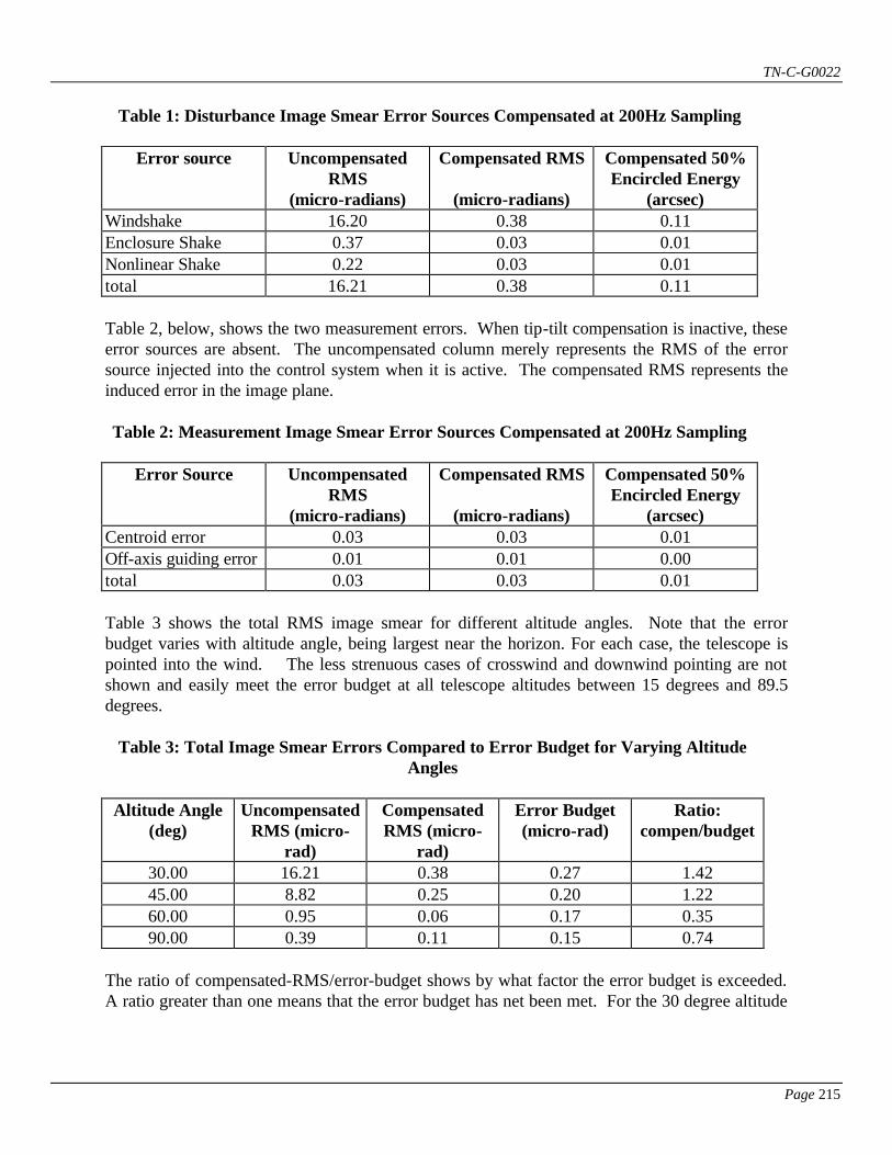
TN-C-G0022

Page 215

Table 1: Disturbance Image Smear Error Sources Compensated at 200Hz Sampling

Error source Uncompensated RMS

(micro-radians)

Compensated RMS

(micro-radians)

Compensated 50% Encircled Energy

(arcsec) Windshake 16.20 0.38 0.11 Enclosure Shake 0.37 0.03 0.01 Nonlinear Shake 0.22 0.03 0.01 total 16.21 0.38 0.11 Table 2, below, shows the two measurement errors. When tip-tilt compensation is inactive, these error sources are absent. The uncompensated column merely represents the RMS of the error source injected into the control system when it is active. The compensated RMS represents the induced error in the image plane. Table 2: Measurement Image Smear Error Sources Compensated at 200Hz Sampling

Error Source Uncompensated

RMS (micro-radians)

Compensated RMS

(micro-radians)

Compensated 50% Encircled Energy

(arcsec) Centroid error 0.03 0.03 0.01 Off-axis guiding error 0.01 0.01 0.00 total 0.03 0.03 0.01 Table 3 shows the total RMS image smear for different altitude angles. Note that the error budget varies with altitude angle, being largest near the horizon. For each case, the telescope is pointed into the wind. The less strenuous cases of crosswind and downwind pointing are not shown and easily meet the error budget at all telescope altitudes between 15 degrees and 89.5 degrees.

Table 3: Total Image Smear Errors Compared to Error Budget for Varying Altitude Angles

Altitude Angle

(deg) Uncompensated

RMS (micro-rad)

Compensated RMS (micro-

rad)

Error Budget (micro-rad)

Ratio: compen/budget

30.00 16.21 0.38 0.27 1.42 45.00 8.82 0.25 0.20 1.22 60.00 0.95 0.06 0.17 0.35 90.00 0.39 0.11 0.15 0.74

The ratio of compensated-RMS/error-budget shows by what factor the error budget is exceeded. A ratio greater than one means that the error budget has net been met. For the 30 degree altitude

TN-C-G0022

Page 216

case, the direct windshake dominates the compensated error, while for greater altitude angles the enclosure and nonlinear shake terms are as important. 6. POSSIBLE AREAS OF FURTHER RESEARCH If the sampling rate could be raised beyond 200Hz, performance could be made to meet the specification under the current preliminary design. Since the closed-loop RMS is almost inversely proportional to the bandwidth, which is in turn proportional to sampling rate, it seems that if the sampling rate were roughly multiplied by 1.5 (to 300Hz) the specification would be met for the most strenuous 30 degree altitude case. One possible way of increasing the sampling rate would be to add fiber-optic-gyros (FOG's) to important places on the telescope structure to sense the motion caused by wind. The FOG's are known to drift over time, which makes them unsuitable for measuring low frequency tracking error, but they are useful for measuring the high speed changes of the telescope. So the rate information from the FOG could be blended with the low frequency positional information from the WFS by way of a complimentary filter as shown in figure 11. The low-pass filter on the WFS measured error and the high-pass filter on the FOG measured error provide a crossover between the two sensors at the cutoff frequency, arbitrarily chosen as 200rad/sec for the example of figure 11. The FOG in this case has been modeled as having a bandwidth of 1000 rad/sec (159Hz), which is thought to be conservative compared to the 500Hz bandwidth quoted for an FOG made by Litton. The difficulty in this method is in choosing appropriate places on the telescope structure to place FOG's and converting the FOG readings into reliable image plane errors. It is thought that placing 3 axis FOG's near the secondary mirror support, the altitude bearings, and on the mount would give some useful information about telescope motion, and would indirectly allow one to calculate an estimate for the image motion due to windshake. Of course the FOG's would add errors of their own and they would have a finite bandwidth, limiting the increase in sample rate afforded by them. The lag of the FOG's would detract from the phase margin of the closed loop tip tilt system and must be taken into account in the controller design to preserve the 60 degree phase margin. Tilt meters and laser Doppler displacement meters (LDDM's) are possible though less promising alternatives to FOG's. A very similar complementary filter can be built to use the slow information from the wavefront sensor to compensate for the low bandwidth atmospheric turbulence, and a brighter off-axis guide star can be used for windshake. The on-axis WFS would be limited to the 3.5 arcminute science field and so would not have the 90% probability of having a bright enough guide star to operate at 300Hz sampling. However this on-axis WFS would adequately sample the low-frequency windshake and all of the atmospheric turbulence, the latter of which usually rolls off at 1Hz. The off-axis WFS, because of the much larger field, could be run at 300Hz due to the much higher probability of finding a sufficiently bright guide star.

TN-C-G0022

Page 217

TN-C-G0022

Page 218

Appendix A25 To: Rick McGonegal File From: Mike Burns Date: May 19, 1994 Subject: Specification for the Gemini Fast-Focus Secondary System Figure 1 shows the PSD of the pistoning motion of the telescope subject to wind, primary mirror motion and thermal expansion. Figure 2 shows the sum of these three contributors. Among the error sources omitted are A/D conversion from the sensor into the digital filter, D/A conversion error from the digital filter to the actuators, and anisoplanitism errors due to using an off-axis star to measure defocus. Figure 3 shows an approximation to the piston PSD. It was chosen to have the correct RMS before and after compensation and approximately the correct slope. The after compensation results were obtained from a control loop having 200Hz sampling and 25Hz closed-loop bandwidth. The approximate PSD is composed of the four line segments: PSD-pist(f) = 2.4e-6 m^2/Hz for f < 0.00025Hz 1.5e-13 m^2/Hz ------- for 0.00025>f>1 Hz f^2 1.5e-13 m^2/Hz for 1>f >10 Hz 1.5e-11 m^2/Hz ------- for f>10 Hz f^2 Figure 4 shows the power spectrum after compensation by the fast-focus control system. The low frequency disturbances have been removed and the higher ones have been left relatively unchanged. If a sampling rate of only 15Hz were available, a correspondingly lower bandwidth filter (around 3Hz) could be used resulting in the filtered PSD of Figure 5. The RMS due to piston disturbances is higher, as shown in table 2, but not by as much as might be expected from the large difference in sample rate. The reason is that both filters do little to attenuate the large amount of power between 20 and 80Hz. Table 2 also includes the measurement noise associated with focus, which varies with sampling frequency. There is an optimum sampling frequency at which to sample because measurement noise increases with sampling rate and compensated piston motion decreases with sampling.

TN-C-G0022

Page 219

Table 1: Fast-focus Requirements

Sampling Rate Uncompensated Piston Motion

RMS (microns)

Compensated Piston Motion

RMS (microns)

Measurement Noise

RMS (microns)

Delivered Piston Motion

RMS (microns) 15Hz 38.30 2.73 0.69 2.82

200Hz 38.30 1.31 2.70 3.00

TN-C-G0022

Page 220

Appendix A26 To: Rick McGonegal From: Mike Burns Date: May 19, 1994 Subject: Report on Compensating Telescope Piston Motion References: [1] R. McGonegal "Focus Measurement Errors" Technical Note Gemini 8-M

Project, to be published May, 1994. [2] M. Burns "Windshake vs. Sample Rate and Centroid Error vs. Sample

Rate for Tip-Tilt Using an Off-Axis Guide Star" Technical Note Gemini 8-M Project (TN-C-G0013), May 1994.

1. SUMMARY The secondary mirror must move axially several microns in order to compensate for the changing telescope focal length and maintain good image quality. This report describes the servo loop for controlling secondary piston motion and quantifies three major sources of piston motion: wind, thermal effects, and primary mirror bending. The expected defocus is calculated both raw (i.e. before compensation) and compensated. 2. INTRODUCTION The fast-focus control loops acts on the secondary mirror to compensate for the piston motion, stretching and compacting of the telescope along the viewing axis. This report examines and quantifies three major sources of piston motion: wind induced, thermally induced and the effective change in focal length due to flexure of the primary mirror. Among the error sources omitted from this report are A/D conversion error from the sensor into the digital controller, D/A conversion error from the digital controller to the actuators, and focus anisoplanatism due to using an off-axis star for focusing. 3. PISTON ERROR SOURCES Figure 1 shows the power spectral densities of the three main sources of telescope piston motion: wind, thermal and primary. 3.1 Telescope Windshake A complex finite element analysis (FEA) of the telescope structure was performed and the resulting model loaded with wind. The component of wind along the z-axis, that is along the line of sight, tends to change the focal length of the telescope.

TN-C-G0022

Page 221

The piston motion due to windshake is the dominant contributor to error for frequencies above 0.01 Hz, as shown in figure 1. The RMS piston motion due to wind is 6.3 microns RMS. Using the conversion factor that 3 microns of defocus is equivalent to 0.01 arcseconds increase in the 50% encircled energy diameter, uncompensated wind will cause 0.021 arcseconds increase in the 50% encircled energy diameter. 3.2 Thermal Drift A change in temperature of 1 deg C/hour was used to estimate the drift in telescope focus as a power spectrum using a 5/3 power law. Thermal drift has a greater total uncompensated RMS than windshake, but because all of its energy is at very low frequencies, it is easily filtered out. So after compensation thermal drift is a small contributor. The uncompensated RMS piston motion due to thermal drift is 31.7 microns, which is equivalent to 0.106 arcseconds increase in the 50% encircled energy diameter. 3.3 Primary Mirror Wind Buffeting The Gemini optics group provided calculations of the optical surface deformations due to wind loading of the primary mirror. These inputs were combined with an idealized wind spectra to estimate the power spectrum due to wind buffeting. The equivalent motion of the secondary mirror to correct for the focus change due to wind on the primary mirror has an RMS of 20.5 microns, which is equivalent to 0.068 arcseconds increase in the 50% encircled energy diameter. 3.4 Focus Measurement Errors Reference [1] gives measurement noise as a function of sampling rate. The calculations of RMS in Ref [1] are based on using a 4-lenslet array, each of which can measure tilt. Ref [2] shows that the RMS tilt error is expected to be 2.7e-8 rad, based on a 6 arcminute field of view, 200Hz sampling, and a star of visual magnitude 12.6 (consistent with 90% probability of finding such a star within the field of view near the north galactic pole). The wavefront defocus, at 200Hz sampling, is found to have a spatial RMS of 54 nm. The spatial RMS of mirror defocus is found to be 27 nm. And the RMS secondary motion is found to be 2.7 microns at 200 Hz sampling. Since the noise is proportional to squar-root of sampling rate, at 15Hz sampling the RMS secondary motion is 0.69 microns. 4. COMBINED DISTURBANCE POWER SPECTRUM Figure 2 shows the net power spectral density (PSD) which is the sum of the three PSD's from figure 1. Also shown is an approximation to the net PSD which comes from the function defined below over four frequency regions. PSD-pist(f) = 2.4e-6 m^2/Hz for f < 0.00025 Hz 1.5e-13 m^2/Hz

TN-C-G0022

Page 222

---------- for 0.00025 > f > 1 Hz f^2 1.5e-13 m^2/Hz for 1 > f > 10 Hz 1.5e-11 m^2/Hz --------- for f > 10 Hz f^2 The approximate PSD above was chosen to have the same net RMS both before and after compensation by the control system as well as to have approximately the correct rolloff in frequency. 5. CURRENT PISTON CONTROL MODEL Figure 3 shows the block diagram used to model the fast-focus plant and controller. The input is a commanded piston motion, measured in meters. The input is compared to the actual position to get an error signal which is measured and passed to the controller. The controller generates a force which acts upon the plant to produce a new position which is fed back closing the loop. The plant, which translates force to position, has a mass of 50kg, a natural frequency of 6.4Hz and light damping of 0.03. The controller attempts to move the two underdamped plant modes to a higher frequency and better damping. The lead-lag controller helps provide some much needed positive phase near the gain crossover, achieving the desired phase margin of 60 degrees which is equivalent to damping of 0.6. The best closed-loop bandwidth that has been obtained is limited to one eighth of the sampling rate. Higher bandwidths for a given sampling rate suffer more degradation in phase margin due to the delay of sampling and cannot meet the 60 degree phase margin. In this report, the closed-loop bandwidth is defined as the location of the closed loop poles. Some authors define bandwidth to be the 3dB frequency of the Bode plot or the inverse of 2*pi*63%-rise-time. These latter two definitions depend upon system zeros while the definition used in this report is more closely related to what can be expected from a given sampling rate. The fast-focus controller described above will operate together with the tip-tilt controller to control the motion of the secondary mirror. They will operate through the same set of actuators but will have different digital controllers. These different controllers can possibly operate at different sampling rates, and their outputs are to be added together digitally to get a net command to each of the three actuators. Implicit in this design is that the two control modes (tip-tilt vs. fast-focus) are decoupled in the sense that commanding a tilt results in very little focus change and commanding piston results in very little tilt. Strong coupling would degrade performance and require a more complicated control strategy. Conceptually, there is no reason why the tip-tilt mode and piston mode must be coupled. If one thinks of a child's seesaw, tip-tilt corresponds to the difference-mode where one side is pressed down and the other moved up an equal amount and opposite direction. Piston corresponds to

TN-C-G0022

Page 223

sum-mode with both sides of the seesaw moving the same amount and the same direction. As a practical matter, there will be some coupling between the axes due to asymmetries in the mechanisms, but it is not expected to be great. 6. RESULTS The attached figures show the simulated results of compensating piston motion. It is possible that the compensated results quoted here are a bit pessimistic because the controller and plant are the same ones used for the tip-tilt studies. It is possible that one could get better results by tailoring the filter to the disturbance spectrum if the latter is known. Figure 4 shows the RMS piston motion after compensation for different sampling rates. The sampling rate directly effects the achievable closed-loop bandwidth according to the relation bandwidth=sampling-rate/8. Figure 5 shows the compensated piston PSD (linear axes). The 15Hz and 40Hz resonances are prominent. This was obtained using the 4th-order servo-loop plus a lead-lag filter operating at 200Hz sampling rate. This approach might have unnecessarily amplified the peak near 40Hz, giving pessimistic results. Figure 6 shows the filtering function used. For an input near 60Hz, the output will not only fail to be attenuated, but will actually be amplified by a factor of nearly 6 in power. One could build a filter that suffered less amplification at these higher frequencies but provided less attenuation at lower frequencies. The filter strategy used in this paper is rather simplistic and does not attempt to trade off the higher frequency response for lower and get a minimum RMS for every sampling frequency. Such an approach would give a lower RMS curve versus sampling rate than figure 4, but would possibly be overly-optimistic because it would assume that the input power spectrum were very well-known and stationary. Table 1 below shows the net RMS piston motion, in microns, before compensation and after compensation with two possible controllers. The 200Hz sampling rate controller attempts to move the plant poles from their 6Hz underdamped positions to 25Hz with 0.6 damping. The 15Hz sampling rate controller gives up attempting to damp the fast poles and just tries to place its own two poles in an acceptable location. Once measurement noise is root-sum-squared with the compensated piston motion, the 200Hz sampling case is actually worse than for 15Hz.

Table 1: Fast Focus RMS Piston Motion Before and After Compensation Sampling Rate Uncompensated

Piston Motion RMS (microns)

Compensated Piston Motion

RMS (microns)

Measurement Noise

RMS (microns)

Total Delivered Error

RMS (microns) 15Hz 38.30 2.73 0.69 2.82

200Hz 38.30 1.31 2.70 3.00

TN-C-G0022

Page 224

Appendix A27 To: Rick McGonegal File From: Mike Burns Date: May 16, 1994 Subject: Specification for the Gemini Tip-Tilt Secondary System Figure 1 shows TY30, a worst-case power spectral density (rad^2/Hz) of uncompensated image plane errors due to windshake. Also shown is a straight line approximation to the spectrum. The approximation was chosen based on two criteria: 1) that both spectra should have the same RMS error both before and after compensation by a candidate control system; and 2) that both spectra have approximately the same spectral content (i.e. corner frequency and rolloff). The candidate controller used to approximate the closed-loop compensated windshake had a sampling rate of 200Hz and a closed-loop bandwidth of 25Hz. An anti-aliasing filter was included in the design. The case TY30 is for the telescope pointed into the wind and 30 degrees above the horizon. The following straight line approximation is used to represent the PSD for this worst case: PSD30(f) = 2.9e-7 rad^2/Hz for f < 0.0004 Hz 4.7e-14 rad^2/Hz for 0.0004<f<1 Hz ------- f^2 4.7e-14 rad^2/Hz for 1<f<10 4.7e-10 rad^2/Hz for f>10 ------- f^4 Figure 2 shows TY90, a more typical power spectrum of uncompensated windshake. The straight line approximation was chosen as described above. The case TY90 is for the telescope pointed into the wind and at the zenith. The straight line approximation to the PSD for this TY90 case is: PSD90(f) = 1.2e-12 rad^2/Hz for f < 0.05 Hz 2.9e-15 rad^2/Hz for 0.05<f<1 Hz ------- f^2 2.9e-15 rad^2/Hz for 1<f<10

TN-C-G0022

Page 225

2.9e-11 rad^2/Hz for f>10 ------- f^4 Table 1 below shows the RMS image motion both before and after compensation as well as the error budget requirement.

Table 1: Tip-tilt Requirements

Telescope Orientation

Uncompensated Windshake RMS

micro-rad

Compensated Windshake RMS

micro-rad

Error Budget Requirement RMS

micro-rad TY30 worst-case 16.20 0.38 0.27 TY90 typical 0.39 0.10 0.15 Vendor is required to meet the values in the "Compensated Windshake RMS" column of table 1 using the secondary tilt system with the straight line approximations for the worst case and typical conditions. It is a goal to meet the "Error Budget Requirement RMS" column of table 1 for the worst case condition.

TN-C-G0022

Page 226

Appendix A28 To: Rick McGonegal From: Mike Burns Date: June 1, 1994 Subject: Effect of 2-millisecond Delay on Tip-Tilt Secondary Control The attached figures show the effect of increasing the delay in the tip-tilt secondary control loop from 500us to 2000us. Increasing delay in a control loop generally results in sloppier control with more overshoot and a larger response to disturbances. Figure 1 shows the response to a commanded step angle position for the tip-tilt secondary controller. The top plot has the nominal delay of 500us and gives an overshoot of 1.4. The bottom plot shows the effect of increasing the delay to 2000us; overshoot increases to 1.6. The phase margin is another measure of quality for a control loop. A phase margin of 60 degrees is often taken as an acceptable. With 500us delay, figure 2 shows a phase margin of 56 degrees. When the delay is increased to 2000us, figure 3 shows the phase margin is only 46 degrees. Figure 4 shows a comparison of the filtering functions for the 500us and 2000us delay cases. The filtering function would be multiplied by an input power spectrum to obtain the after-compensation image plane error. It is desired to have a smaller filtering function to attenuate disturbances. It can be seen in figure 4 that both filtering functions are very small for disturbances below 10Hz. However near 50Hz the 2000us delay loop has much worse performance than the 500us delay loop. At 50Hz, the input disturbance is not only failed to be attenuated, but is actually amplified by a factor of 11 in power (6.5 for the 500us case).

TN-C-G0022

Page 227

Appendix A29 & A30 To: Rick McGonegal From: Mike Burns Date: June 2, 1994 Subject: Windshake vs. Sample Rate and Centroid Error vs. Sample Rate for Tip-Tilt

Using an Off-Axis Guide Star (updated) References: [1] Ulich, Bobby L. "Overview of Acquisition, Tracking and Pointing System Technology" Proceedings SPIE 1988. Acquisition, Tracking and Pointing II. pp40-63. [2] Burns, Mike "SNR vs. Sample Rate for Tip-Tilt Using an Off-Axis Guide Star" Technical Note, Gemini 8-M Telescopes Project. August 1993. [3] Burns, Mike "Windshake vs. Sample Rate and Centroid Error vs. Sample Rate for Tip-Tilt Using an Off-Axis Guide Star", Technical Note, Gemini 8-M Telescopes Project, August 1993. 1. SUMMARY Using the 3.5 arcminute diameter science field to find a bright star with which to compensate for windshake meets the error budget over most of the sky with a sampling rate of 200Hz. Only the cases pointed into the wind and near the horizon (labeled TY30 and TY90 in the text) are not met with a 3.5 arcminute diameter field. In these cases, even an 11.5 arcminute diameter field does not make the error budget because the error is dominated by the windshake and only little affected by the centroid error. From [2] the 3.5 arcminute diameter field provides neither attenuation nor amplification of atmospheric induced tip-tilt error. More recently, information from Brent Ellerbroek of Starfire Labs seems to indicate that a 6.0 arcminute diameter field without suffering an increase in the atmospheric induced tip-tilt error. This larger field will guarantee a brighter guide star and reduce the centroid measurement error. The centroid measurement error is a significant contributor to image smear over much of the sky. Unfortunately, the TY30 and TY45 cases are dominated by windshake and will not be significantly helped by the reduction in centroid error. 2. INTRODUCTION The results presented here are updated from Ref [3]. Building on the earlier note of SNR vs. Sample Rate, this note computes the disturbance shake of the telescope and the RMS centroid error vs. sample sate and root sum squares (RSS) them to

TN-C-G0022

Page 228

calculate a net RMS error. Note that the errors are ignored which result from atmospheric decorrelation due to spatial difference between guide star and science object. 3. TIP-TILT ERROR SOURCES There are two types of image smear error sources to be considered, disturbances and measurement noise. Figure 1 helps distinguish between these. The three disturbances as the far left of figure 1 can be though of as commanded positions for the secondary mirror. These commands are compared to the actual secondary position to get the true tracking error. The true tracking error is corrupted by additive measurement noise to give the measured tracking error. The controller acts upon the measured tracking error to supply a torque through the actuators to the secondary mirror, changing its position and closing the loop. It can be seen that for a purely open loop case, if the controller were removed, the only errors that would be noticed would be the disturbance errors at the far left of figure 1. The measurement errors only affect tracking when the loop is closed. The following sections describe in some detail the individual disturbances (windshake, enclosure shake and nonlinear control system shake) and the measurement errors (centroid noise and off-axis guiding error). 3.1 Windshake The RMS windshake was calculated by using a finite element analysis (FEA) to produce a spectrum of image motion due to the direct effect of wind upon the telescope structure. The spectrum of figure 2 is in the form of a power spectral density, radians^2/Hz vs. frequency. Integrating the spectrum over frequency gives angular noise power. Taking the square root then gives the RMS image centroid motion due to windshake without any correction by the servo loop. If the windshake spectrum is passed through a filter, representing the servo system, then a spectrum "after compensation" results. This latter spectrum will typically have less energy in the lower frequencies because the servo system is capable of tracking these slower moving disturbances. The "after compensation" spectrum may be integrated and the square root gives the compensated windshake RMS image centroid motion. The servo in this case is assumed to be a sampled data system with bandwidth equal to 1/8th of the sampling frequency. The servo loop is 4th order and includes an anti-aliasing filter to prevent the noise associated with sampling from being "folded-back" into the filter. There is also a lead-lag filter to improve the phase margin near the gain-crossover frequency. Higher bandwidth is desirable, but is limited to sampling/8 by the restriction of maintaining 60 degrees of phase margin. The motion of the telescope tube due to wind is dependent upon the altitude of the tube above the horizon and upon the direction of wind relative to the telescope. Many different wind cases are listed in Table 1 of the results section below. The cases labeled TY# are for the telescope pointed into the wind at an angle # degrees above the horizon. The cases labeled TX# are for the

TN-C-G0022

Page 229

telescope pointed across the wind at an angle # degrees above the horizon. The into the wind cases are the most difficult for which to meet the error budget. 3.2 Enclosure Induced Shake Another effect associated with wind is the motion of the telescope enclosure which is transmitted through the pier and then to the telescope tube, causing image smear. Figure 3 shows the uncompensated spectrum for this effect, which is expected to be nearly independent of wind direction. 3.3 Nonlinear Control System Induced Shake The control system will be imperfect and will contribute to error in the image plane. Among the nonlinear errors are altitude and azimuth axis encoder quantizations, bearing frictions, motor torque noise (both cogging and torque constant variation), tachometer ripple, motor D/A conversion error, and drive wheel eccentricities. Figure 4 shows the uncompensated spectrum for these in both the x and y image directions for a typical case. 3.4 Centroiding Measurement Noise The wavefront sensor can not perfectly compute the image centroid. This section quantifies the centroid errors which are plotted in figure 5 for a 200Hz sampling rate. From ref [1] the full width half max error is given by fwhm = 0.995 * A^(3/5) * lambda / R0 where A = 1 lambda = 0.7e-6 m = wavelength of interest R0 = 0.3 m = aperture . From reference [2] the SNR is given as a function of sampling rate and field diameter. The centroid error is given in [1] as a function of the fwhm and the SNR of ref [2] by sig_centroid = [4*ln(2)]^(-0.5) * fwhm / SNR 3.5 Off-Axis Guiding Error Another measurement error is due to the fact that the guide star and science object are not both in the center of the field. Since the cassegrain rotator control system is imperfect, there will be a net RMS error in the cassegrain position. This rotational error of the field will make the guide object appear to move, and when the control system tracks the guide object, the error will be induced in

TN-C-G0022

Page 230

the science object. Figure 6 shows the spectrum of the induced error in the image plane due to off-axis tracking. 3.6 Combined Error Spectra The windshake, enclosure shake, and nonlinear control system induced shake are combined to give a total disturbance spectrum as shown in figure 7. This is for the worst case, TY30, and can be seen to be dominated by the windshake by comparing with figure 2. Figure 8 shows the combined measurement noise spectra from figures 5 and 6, and can be seen to be dominated by the centroid error of figure 5. 4 RESULTS There is a competition between disturbance errors and measurement errors. For a low sampling rate, and therefore a low system bandwidth, disturbance errors dominate the compensated RMS error. As sampling rate is increased, disturbance errors are reduced but measurement errors increase. For a given field diameter, there is an optimum sample rate which gives a minimum total RMS image plane error. Figures 9 through 18 show the results versus sampling rate for the 10 different cases studied. Using figure 9 as an example, the two plots at the top of the page show the dominant error sources: windshake and centroid error vs. sampling rate. These two dominant effects are added, together with the lesser contributors described in section 3 above, to give the total RMS image plane error in the lower left of figure 9. Table 1 summarizes the results for the 10 different wind cases, comparing the error budget with the minimum diameter necessary to meet the error budget (assuming that a sufficiently high sample rate were available). The cases labeled TY30 and TY45 are noticed to be very difficult, requiring about twice the available 200Hz sampling rate. The first column of table 1 shows the wind case studied. The cases labeled TX# are crosswind cases with the telescope pointed # degrees above the horizon. The cases labeled TY# are looking into the wind and # degrees above the horizon. The second column of table 1 shows the error budget in microradians of RMS image centroid motion that is tolerable. The third column shows that diameter of guide field, in arcminutes, which theoretically could just barely meet the error budget at some sampling rate. The required sampling rate is sometimes quite high, as shown in column 5. For any given guide field diameter, there is a stellar visual magnitude such that there is a 90% probability of finding at least one star of that minimum brightness within the guide field. Column 4 shows the stellar visual magnitude based on the guide field diameter of column 3. The last column, column 6, shows that if the guide field were increased to 11.5 arcminutes the required sampling rates would be reduced. This is because a larger guide field would likely have a brighter guide star, which would reduce the amount of image smear due to the centroid calculation noise.

TN-C-G0022

Page 231

For the crosswind cases, labeled TX# in table 1, the required sampling rate increases with altitude angle because the error budget decreases near the zenith. For the cases where the telescope is pointed into the wind, labeled TY# in table 1, the required sampling rate is higher for the lower altitude cases. Unlike the crosswind cases, the secondary support structure presents a larger surface to the wind at low altitude angles, which gathers more energy and causes more image plane motion.

Table 1: Field Diameters and Star Brightness Needed to Meet Error Budget for Different Cases of Wind

Wind Case Error Budget

(microrads)

D_90 Min diameter to meet error-

budget

(arcminutes)

Stellar Mag required

given D_90

(absolute)

Sample freq for D_90 to meet error-

budget

(Hz)

Sample freq for 11.5

arcmin to meet

error-budget (Hz)

TX15 0.43 2.4 21.4 80 50 TX30 0.28 2.3 21.7 120 65 TX45 0.21 2.4 21.4 130 80 TX60 0.18 2.5 21.2 150 90 TX75 0.16 2.7 20.8 170 100 TX90 0.16 2.7 20.8 170 100 TY30 0.28 2.9 20.4 400 280 TY45 0.21 2.9 20.4 350 250 TY60 0.18 2.5 21.2 150 90 TY90 0.16 2.9 20.4 200 120

The results of table 1 as well as figures 9 through 18 were obtained with the Matlab programs correl4.m and correl4b.m in the mburns directory c:\matlab\wind\.

TN-C-G0022

Page 232

Appendix A31 To: Rick McGonegal (8M) CC: Richard Kurz (8M) CC: Peregrine McGehee (8M) CC: Matt Mountain (8M) CC: Jim Oschmann (8M) CC: David Robertson (8M) CC: Doug Simons (8M) CC: Malcolm Stewart (ROE) CC: Magnus Patterson (ROE) CC: Nick Dillon (RGO) CC: Dave Gellatly (RGO) CC: Charles Jenkins (RGO) CC: Robert Laing (RGO) From: Mike Burns Date: June 8, 1994 Subject: Compensated Windshake Results for Tip-tilt with Integration Delay SUMMARY The effect upon the tip-tilt control loop of various delays is to harm the phase margin and cause a larger RMS tracking error. Three sources of delay are considered: CCD integration time, numerical processing delay, and a sample-and-hold. Results are quoted for varying the numerical processing delay from 0ms to 5ms. A processing delay of 0.5ms is acceptable, but larger delays are probably not. SIMULATION DESCRIPTION Figure 1 shows a block diagram for the simulation used in this memo. The input disturbance, in this case windshake, can be thought of as a commanded angular position for the secondary mirror. It is compared to the actual secondary position, labeled theta, to get a real error signal. The root mean square (RMS) of this error signal over time represents the performance measure of the tip-tilt secondary. The true error signal passes through a delay representing the effect of integration within the charge coupled devices (CCD's) plus some small processing delay. The error signal is then passed to a digital filter with an implied sample-and-hold. In this simulation, the digital filtering is composed of a lead-lag filter and a second-order proportional-integral (PI) controller. The controller commands a torque which acts upon the plant and anti-aliasing filter to produce change theta, the angle of the secondary mirror, thus closing the loop.

TN-C-G0022

Page 233

The plant is modeled as having a moment of inertia of 4 kg-m^2, a natural frequency of around 6.4Hz and light damping of about 3%. The simulation operates in the frequency domain. A transfer function is computed from disturbance in to error out. This transfer function is multiplied by an input power spectrum (rad^2/Hz) to get a power spectrum after compensation. The resulting power spectrum is integrated over frequency, and the square root gives an RMS tracking error in radians. The effect upon the tip-tilt control loop of the various delays is to harm the phase margin which in turn lowers the achievable bandwidth for a given sampling frequency. A lower bandwidth results in the tip-tilt loop removing less of the disturbance and ultimately causes a larger tracking error. Even if a control loop with a poor phase margin seemed to give acceptable performance in the simulation, it would still not be advisable to build such a system. A system with low phase margin is not robust and can be easily made to ring or become unstable. For this analysis, the system was designed for a phase margin of 60 degrees and a gain margin of 3 dB. This is near the edge of what could be considered good control design. Some engineers prefer more generous margins of 70 degrees and 6 dB. There are three sources of delay between the existence of a true tracking error and the application of a correcting torque upon the secondary mirror. The CCD's must integrate the error signal. Since the loop is assumed to operate at 200Hz, the average time delay due to integration is half of a period, or 2.5ms. Next there is the delay associated with numerical processing, which was varied between the nominal value of 0.5ms and an upper limit 5ms for this study. A third source of delay is the required sample and hold after the integrator at the input to the digital filter. The sample-and-hold ads about half of a period, or 2.5ms of delay. Figure 2 shows the effect of the various delay sources. The upper left plot shows an input signal, representing image plane error in microradians for example. The upper right shows the corresponding output from the CCD, modeled as an integrator which is reset at 200Hz and scaled appropriately. The lower left plot shows the effect of a sample and hold and the lower right plot ads a bit more delay to account for the numerical processing. RESULTS Table 1 shows the compensated RMS windshake as a fraction of the error budget for the simulated tip-tilt loop. The error budget includes the effect of direct windshake and indirect windshake through the enclosure, but does not take into account the centroid measuring error, which is expect to be small (i.e. 0.027 microradians) compared to the other terms. The telescope is assumed to be pointed into the wind and the altitude axis is varied from 30 degrees above horizon to 90 degrees (i.e. zenith pointing). The direct effect of wind upon the telescope topend is the dominant source of motion in the image plane, but the indirect effect of wind upon the enclosure has also been included.

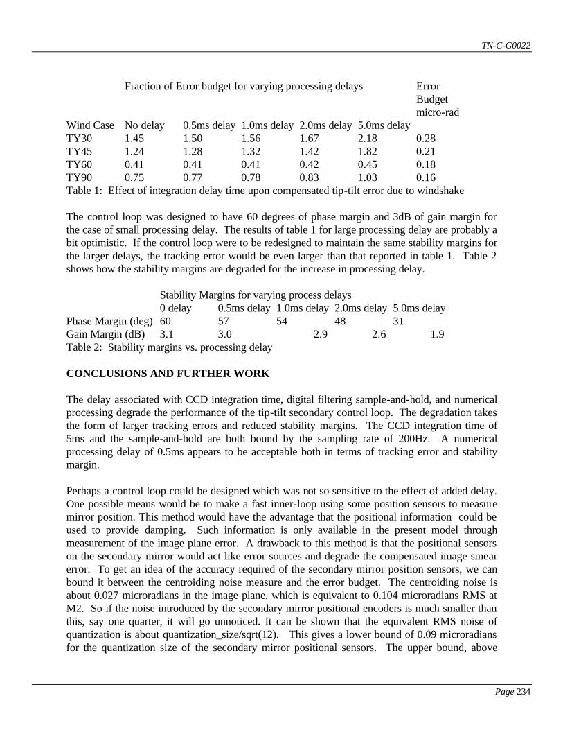
TN-C-G0022

Page 234

Fraction of Error budget for varying processing delays Error

Budget micro-rad

Wind Case No delay 0.5ms delay 1.0ms delay 2.0ms delay 5.0ms delay TY30 1.45 1.50 1.56 1.67 2.18 0.28 TY45 1.24 1.28 1.32 1.42 1.82 0.21 TY60 0.41 0.41 0.41 0.42 0.45 0.18 TY90 0.75 0.77 0.78 0.83 1.03 0.16 Table 1: Effect of integration delay time upon compensated tip-tilt error due to windshake The control loop was designed to have 60 degrees of phase margin and 3dB of gain margin for the case of small processing delay. The results of table 1 for large processing delay are probably a bit optimistic. If the control loop were to be redesigned to maintain the same stability margins for the larger delays, the tracking error would be even larger than that reported in table 1. Table 2 shows how the stability margins are degraded for the increase in processing delay. Stability Margins for varying process delays 0 delay 0.5ms delay 1.0ms delay 2.0ms delay 5.0ms delay Phase Margin (deg) 60 57 54 48 31 Gain Margin (dB) 3.1 3.0 2.9 2.6 1.9 Table 2: Stability margins vs. processing delay CONCLUSIONS AND FURTHER WORK The delay associated with CCD integration time, digital filtering sample-and-hold, and numerical processing degrade the performance of the tip-tilt secondary control loop. The degradation takes the form of larger tracking errors and reduced stability margins. The CCD integration time of 5ms and the sample-and-hold are both bound by the sampling rate of 200Hz. A numerical processing delay of 0.5ms appears to be acceptable both in terms of tracking error and stability margin. Perhaps a control loop could be designed which was not so sensitive to the effect of added delay. One possible means would be to make a fast inner-loop using some position sensors to measure mirror position. This method would have the advantage that the positional information could be used to provide damping. Such information is only available in the present model through measurement of the image plane error. A drawback to this method is that the positional sensors on the secondary mirror would act like error sources and degrade the compensated image smear error. To get an idea of the accuracy required of the secondary mirror position sensors, we can bound it between the centroiding noise measure and the error budget. The centroiding noise is about 0.027 microradians in the image plane, which is equivalent to 0.104 microradians RMS at M2. So if the noise introduced by the secondary mirror positional encoders is much smaller than this, say one quarter, it will go unnoticed. It can be shown that the equivalent RMS noise of quantization is about quantization_size/sqrt(12). This gives a lower bound of 0.09 microradians for the quantization size of the secondary mirror positional sensors. The upper bound, above

TN-C-G0022

Page 235

which performance would clearly be unacceptable is the error budget. The error budget at zenith is 0.158 microradians RMS in the image plane, or 0.61 microradians motion of M2. This leads to an acceptable quantization step size of 0.61*sqrt(12)=2.1 microradians. So it would seem that if the secondary mirror position sensors had smaller error than 0.09 microradians, they would go unnoticed, and if they had a larger error than 2.1 microradians the results would be guaranteed to be unacceptable. In the region between 0.09 and 2.1 microradians, further study would be required to quantify the tradeoff between better damping and the increased noise due to positional measurement error. Another possible method would be to use fiber optic gyros (FOG's) to obtain high frequency windshake motion, and lower the required sampling rate. A complimentary filter would be implemented to blend the high-frequency information from the FOG with low frequency information from the wavefront sensor. A lower sampling rate results in proportionately less phase margin degradation for a given delay time.

TN-C-G0022

Page 236

Appendix A32 To: Perrigrine Mcgehee CC: Rick McGonegal From: Mike Burns Date: June 9, 1994 Subject: Mount Control Motor Parameters Here is my estimation of the motor parameters you asked about. The attached block diagram shows how I imagine the information to flow around the servo loop. The analog motor board gets a motor rate command (not a current command) from the digital filter. This rate command is through a 16-bit D/A converter, so the resolution is max_rate/2^16, which is around 2.6e-5 rad/sec. It is possible that this will be a 12-bit encoder. The tachometer is an analog device and it is kept in an analog loop, so there seems to be no need to digitize it, therefore the resolution is meaningless. It does have an analog noise of about 0.1% of signal. The maximum rate for this tachometer is 47 rad/sec = 450 RPM, which is quite large for our purposes. The encoders which measure mount position are expect to have a resolution of 4.7e-8 radians and a limit of +/- pi radians. The analog motor board uses encoders to measure the position of the motor shaft in order to smoothly commutate the motor. I do not know what the resolution is on these encoders. The motor vendor will choose these. The specification is that these encoders will be whatever is necessary to limit the motor torque variation to 2%.

TN-C-G0022

Page 237

Appendix A33 1. IMAGE SMEAR ERROR BUDGET The image smear error budget is item 1.3 of the image quality error budget and represents those error budget items which cause the centroid of the image to move during the detector integration time. The baseline value of the top level error budget is 0.03 arcseconds increase in 50% encircled energy (f/16, 2.2 microns, 1 arcminute field, zenith pointing, 70th percentile wind). This error budget is zenith angle dependent as the top level image quality error budget increases with zenith angle. The current allocation is: Zenith Angle Error Budget

(50% encircled energy) Error Budget

(image centroid) degrees arcseconds microradians arcseconds microradians

0.00 0.04 0.21 0.03 0.16 15.00 0.05 0.22 0.03 0.16 30.00 0.05 0.24 0.04 0.18 45.00 0.06 0.29 0.04 0.21 60.00 0.08 0.37 0.06 0.28 75.00 0.12 0.58 0.09 0.43

The translation of the science error budget in terms of 50% encircled energy has been translated to an engineering error budget in terms of image centroid rms movement. This is done as all of the analysis of the tracking of the telescope is more naturally done in terms of image centroid rms. The relationship adopted for going from 50% encircled energy to image centroid rms has been detailed elsewhere (reference). The relationship is: E(50%) = 1.35 * E(rms) This relationship is based on calculating the 50% encircled energy diameter of a gaussian curve with unity rms. The relationship is based on calculating the 50% encircled energy from image centroid rms where the motion is sinusoidal is assumed to be: E(50%) = 2.0 * E(rms) This relationship comes from work by John Roberts based on Code V. The breakdown of the error budget into its major parts is detailed in the table below:

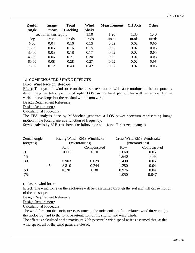
TN-C-G0022

Page 238

Zenith Angle

Image Smear

Total Tracking

Wind Shake

Measurement Off Axis Other

section in this report 1.10 1.20 1.30 1.40 deg arcsec urads urads urads urads urads 0.00 0.04 0.16 0.15 0.02 0.02 0.05

15.00 0.05 0.16 0.15 0.02 0.02 0.05 30.00 0.05 0.18 0.17 0.02 0.02 0.05 45.00 0.06 0.21 0.20 0.02 0.02 0.05 60.00 0.08 0.28 0.27 0.02 0.02 0.05 75.00 0.12 0.43 0.42 0.02 0.02 0.05

1.1 COMPENSATED SHAKE EFFECTS Direct Wind force on telescope Effect: The dynamic wind force on the telescope structure will cause motions of the components determining the telescope line of sight (LOS) in the focal plane. This will be reduced by the various servo loops but the residual will be non-zero. Design Requirement Reference: Design Requirement: Calculational Procedure: The FEA analysis done by M.Sheehan generates a LOS power spectrum representing image motion in the focal plane as a function of frequency. Servo analysis by M.Burns shows the following results for different zenith angles Zenith Angle (degrees)

Facing Wind RMS Windshake (microradians)

Cross Wind RMS Windshake (microradians)

Raw Compensated Raw Compensated 0 0.110 0.10 1.660 0.05 15 1.640 0.050 30 0.903 0.029 1.490 0.05

45 8.810 0.244 1.280 0.04 60 16.20 0.38 0.976 0.04 75 1.050 0.047 enclosure wind force Effect: The wind force on the enclosure will be transmitted through the soil and will cause motion of the telescope. Design Requirement Reference: Design Requirement: Calculational Procedure: The wind force on the enclosure is assumed to be independent of the relative wind direction (to the enclosure) and to the relative orientation of the shutter and wind blinds. The effect is calculated at the maximum 70th percentile wind speed as it is assumed that, at this wind speed, all of the wind gates are closed.

TN-C-G0022

Page 239

Uncompensated Enclosure-Induced Image-Error (microrad)

Compensated Enclosure-Induced Image Error (microrad)

0.37 0.03 See Appendix A for M. Sheehan's memo comparing the transfer functions of M. Sheehan's model with M. Burns' model. [see work by M.Sheehan/M.Burns] enclosure bogies Effect: The vibration of the enclosure bogie wheels as the enclosure is rotated will cause motion of the telescope. Design Requirement Reference: Design Requirement: Calculational Procedure: Just as the direct wind force and enclosure wind force errors are reduced by the tip-tilt control loop, so will the disturbances caused by the enclosure bogies. [see work by M.Sheehan/M.Burns] measurement error Effect: The brightness of the star available for use as a guide signal will act as a noise source. Design Requirement Reference: Design Requirement: Calculational Procedure: [this work should be replaced by more detailed calculations of B.Ellerbroek/C.Jenkins] There are a number of steps needed to calculate the noise equivalent angle of the guide star: the diameter of the guide field determines the brightness of the star available (90% probability at galactic pole) the physical constants of the detector combined with the sampling rate determine the signal/noise of the detected signal the S/N is used to determine the centroiding error according to the equation: sig_centroid = [4*ln(2)]-0.5 * fwhm / SNR where the fwhm is the full width half max error in radians. The following table shows the required visual magnitude for three field diameters such that there is a 90% chance of finding a star of the given magnitude or brighter. The three diameters are 2.4 arcminutes (representing that diameter at which atmospheric tip-tilt may be reduced by a factor of 2), 3.5 arcminutes (representing the edge of the science field), and 7.2 arcminutes (representing the equivalent diameter of the annulus surrounding the science field and within the guide field). Item Field Diameter (arcminutes) 2.40 3.50 8.0 Visual magnitude 21.50 19.40 15.40 SNR 3.70 9.70 61.60 centroid error (microradians)

0.27 0.10 0.02

TN-C-G0022

Page 240

off axis guiding errors Probe Flexure Effect: The use of a probe to measure the centroid of an off axis guide star will result in the relative flexure between probe and the science detector showing up as image smear over the integration time (1 hour). Design Requirement Reference: Design Requirement: Calculational Procedure: [see work by C.Jenkins] anisoplanicity Effect: The use of an off axis guide star will result in the decorrelated part of the image motion due to atmospheric turbulence manifesting itself as additional image smear in the science object over the integration time (1 hour). Design Requirement Reference: Design Requirement: Calculational Procedure: [see work by C.Jenkins & B.Ellerbroek] field rotation errors Effect: The use of an off axis guide star will result in field rotation errors in the guide object being injected into the science object tracking. Design Requirement Reference: Design Requirement: Calculational Procedure: Servo analysis by M.Burns shows the following results. State Value (urads) Raw Value 8e-3 After Tip/Tilt 8e-3 Error Budget 8e-3 other compensated errors compensated altitude errors altitude bearing Effect: The altitude bearing will have viscous, coulomb and stiction friction components. There is also a random component which is modeled as having an RMS of 0.7 times the coulomb friction and a time constant of 2 seconds, per conversation with Martin Fischer of RGO. Although these errors will be reduced by the servo system there will be a residual. Design Requirement Reference: Design Requirement: Calculational Procedure: Servo analysis by M.Burns shows the following results. State Value (urads) Raw Value 5.0e-2

TN-C-G0022

Page 241

After Tip/Tilt 2.2e-2 Error Budget altitude drive ripple Effect: Commutation will cause the output torque of the drive motors to vary at relatively high frequency. Design Requirement Reference: Design Requirement: Calculational Procedure: Servo analysis by M.Burns shows the following results. State Value (urads) Raw Value 1.5e-2 After Tip/Tilt 1.2e-2 Error Budget altitude quantization Effect: The resolution of the altitude encoder will cause a tracking error. Design Requirement Reference: Design Requirement: Calculational Procedure: Servo analysis by M.Burns shows the following results. State Value (urads) Raw Value 3.3e-2 After Tip/Tilt 2.8e-3 Error Budget Altitude Drive Eccentricity Effect: The variation from a perfect circle will cause the drive wheel to have a torque which varies with rotational angle. This will cause non-uniform tracking and result in a tracking error. Design Requirement Reference: Design Requirement: Calculational Procedure: Servo analysis by M. Burns shows the following results State Value(urad) Raw Value 1.4e-3 After Tip/Tilt 5.3e-4 Error Budget Altitude Tachometer Errors Effect: The altitude drive motors rely on tachometers in order to smoothly commutate. These tachometers have a ripple voltage which varies with rotational angle, introducing ripple in the drive motors and leading to tracking error.

TN-C-G0022

Page 242

Design Requirement Reference: Design Requirement: Calculation Procedure: Servo Analysis by M. Burns shows the following results. State Value(urad) Raw Value 3.0e-3 After Tip/Tilt 5.3e-4 Error Budget Altitude Motor D/A Quantization Errors Effect: A digitally implemented controller issues a commanded rate to the altitude drive motors. The rate must be converted from the digital domain to a real voltage by means of a D/A converter which has a finite number of bits. The resulting noise on the motor command leads to tracking errors. Design Requirement Reference: Design Requirement: Calculation Procedure: Servo Analysis by M. Burns shows the following results. State Value(urads) Raw Value 4.6e-2 After Tip/Tilt 1.9e-2 Error Budget Altitude Pointing Effect: The flexures, etc. that cause altitude pointing errors will show up as tracking errors during an exposure. Design Requirement Reference: Design Requirement: Calculational Procedure: Previous analysis done for the primary mirror PDR has estimated the contribution to raw image quality due to telescope flexures as 3.138 arcseconds 50% encircled energy over an hour exposure. If we translate this to rms image centroid motion, 2.324 arcseconds / 11.27 uradians, and then assume that azimuth and altitude equally contribute to this, we get a value of 7.969 uradians as the altitude pointing contribution. The same analysis shows that, after tip/tilt correction, these flexure errors would be reduced to 0.002 arcseconds 50% encircled energy. Going through the same calculation yields 0.005 uradians residual error. State Value (urads) Raw Value 7.97 After Tip/Tilt 0.01 Error Budget compensated azimuth errors

TN-C-G0022

Page 243

azimuth bearing Effect: The azimuth bearing will have viscous, coulomb and stiction friction components. Although these will be reduced by the servo system there will be a residual. Design Requirement Reference: Design Requirement: Calculational Procedure: Servo analysis by M.Burns shows the following results. State Value (urads) Raw Value 1.3e-2 After Tip/Tilt 3.1e-3 Error Budget azimuth drive ripple Effect: Quantization, torque commutation will cause the output of the azimuth drive motors to vary at relatively high frequency. Design Requirement Reference: Design Requirement: Calculational Procedure: Servo analysis by M.Burns shows the following results. State Value (urads) Raw Value 1.4e-2 After Tip/Tilt 1.1e-2 Error Budget azimuth quantization Effect: The resolution of the azimuth encoder will cause a tracking error. Design Requirement Reference: Design Requirement: Calculational Procedure: Servo analysis by M.Burns shows the following results. State Value (urads) Raw Value 1.3e-2 After Tip/Tilt 2.9e-3 Error Budget Azimuth Drive Eccentricity Effect: The variation from a perfect circle will cause the drive wheel to have a torque which varies with rotational angle. This will cause non-uniform tracking and result in a tracking error. Design Requirement Reference: Design Requirement: Calculational Procedure: Servo analysis by M. Burns shows the following results State Value(urads) Raw Value 1.1e-3 After Tip/Tilt 5.3e-4

TN-C-G0022

Page 244

Error Budget Azimuth Tachometer Errors Effect: The azimuth drive motors rely on tachometers in order to smoothly commutate. These tachometers have a ripple voltage which varies with rotational angle, introducing ripple in the drive motors and leading to tracking error. Design Requirement Reference: Design Requirement: Calculation Procedure: Servo Analysis by M. Burns shows the following results. State Value(urads) Raw Value 1.6e-3 After Tip/Tilt 5.3e-4 Error Budget Azimuth Motor D/A Quantization errors Effect: A digitally implemented controller issues a commanded rate to the azimuth drive motors. The rate must be converted from the digital domain to a real voltage by means of a D/A converter which has a finite number of bits. The resulting noise on the motor command leads to tracking errors. Design Requirement Reference: Design Requirement: Calculation Procedure: Servo Analysis by M. Burns shows the following results. State Value(urads) Raw Value 2.0e-2 After Tip/Tilt 1.4e-2 Error Budget Azimuth Pointing Effect: The flexures, etc. that cause azimuth pointing errors will show up as tracking errors during an exposure. Design Requirement Reference: Design Requirement: Calculational Procedure: See previous explanation for altitude pointing. State Value (urads) Raw Value 7.97 After Tip/Tilt 0.01 Error Budget compensated cassegrain rotator errors cassegrain bearing Effect: Design Requirement Reference:

TN-C-G0022

Page 245

Design Requirement: Calculational Procedure: Servo analysis by S. Wieland shows the following results. State Value (urads) Raw Value 3.96e-2 After Tip/Tilt 2.8e-3 Error Budget slow cassegrain errors Pinion Eccentricity Effect: The pinion which drives the cassegrain rotator will have a measurable eccentricity. Design Requirement Reference: Design Requirement: Calculational Procedure: Analysis by the instrument group has shown the following: State Value (urads) Raw Value 0.02 After Tip/Tilt 0.00 Error Budget As these are slowly varying errors we have estimated that the tip tilt system will remove 95% of them. drum eccentricity Effect: The drum against which the pinion drives will have a measurable eccentricity. Design Requirement Reference: Design Requirement: Calculational Procedure: Analysis by the instrument group has shown the following: State Value (urads) Raw Value 0.02 After Tip/Tilt 0.00 Error Budget As these are slowly varying errors we have estimated that the tip tilt system will remove 95% of them. guide probe Effect: The guide probe used to hold the A&G detector will have a measurable flexure. This will result in tracking errors as there will be motion introduced between the guide object and the science object. Design Requirement Reference: Design Requirement: Calculational Procedure: Analysis by the instrument group has shown the following: State Value (urads) Raw Value 0.02

TN-C-G0022

Page 246

After Tip/Tilt 0.00 Error Budget As these are slowly varying errors we have estimated that the tip tilt system will remove 95% of them. drive windup Effect: There will be a measurable backlash in the drive system. Design Requirement Reference: Design Requirement: Calculational Procedure: Analysis by the instrument group has shown the following: State Value (urads) Raw Value 0.00 After Tip/Tilt 0.00 Error Budget As these are slowly varying errors we have estimated that the tip tilt system will remove 95% of them. cassegrain pointing Effect: The flexures, etc. that cause the focal plane to move during an exposure will result in tracking errors. Design Requirement Reference: Design Requirement: Calculational Procedure: Although the rotation axis of the cassegrain rotator is defined as the pointing datum for the telescope there will be, during an exposure, motion of that plane relative to the other cardinal axes of the telescope. Although the goal of the telescope control system is to track the cassegrain rotator axis on the science object, and to track the primary/secondary optical axes to the cassegrain rotator axis, there will be residual, uncorrected motions during an exposure which will move the image centroid. If we look at the analysis done for pointing we find that there is 1.391 arcseconds/6.744 uradians due to motion of the focal plane over the entire sky. If we assume that only 1/6 of this will show up during a 1 hour exposure and that 98% of the effect will be removed by the tip/tilt system then we have the following. State Value (urads) Raw Value 6.74 During 1 hr 1.12 After Tip/Tilt 0.02 Error Budget cassegrain encoder Effect: The resolution of the cassegrain encoder will cause the field to rotate non-uniformly. Design Requirement Reference: Design Requirement: Calculational Procedure:

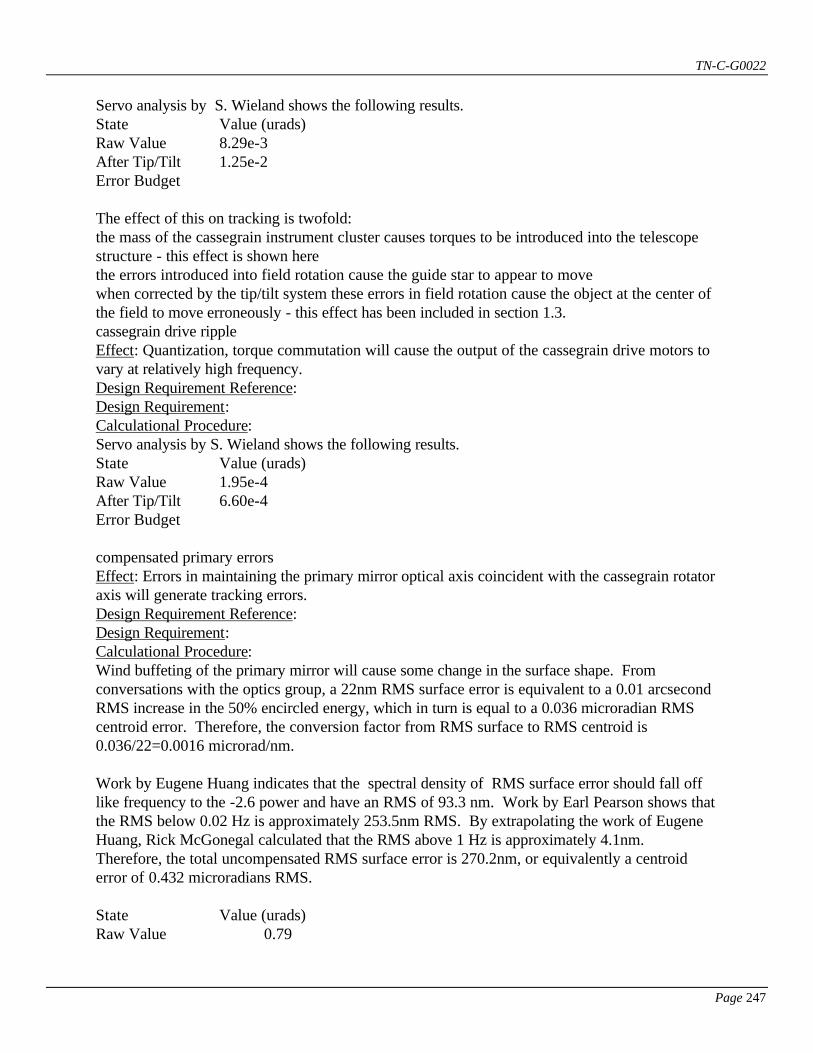
TN-C-G0022

Page 247

Servo analysis by S. Wieland shows the following results. State Value (urads) Raw Value 8.29e-3 After Tip/Tilt 1.25e-2 Error Budget The effect of this on tracking is twofold: the mass of the cassegrain instrument cluster causes torques to be introduced into the telescope structure - this effect is shown here the errors introduced into field rotation cause the guide star to appear to move when corrected by the tip/tilt system these errors in field rotation cause the object at the center of the field to move erroneously - this effect has been included in section 1.3. cassegrain drive ripple Effect: Quantization, torque commutation will cause the output of the cassegrain drive motors to vary at relatively high frequency. Design Requirement Reference: Design Requirement: Calculational Procedure: Servo analysis by S. Wieland shows the following results. State Value (urads) Raw Value 1.95e-4 After Tip/Tilt 6.60e-4 Error Budget compensated primary errors Effect: Errors in maintaining the primary mirror optical axis coincident with the cassegrain rotator axis will generate tracking errors. Design Requirement Reference: Design Requirement: Calculational Procedure: Wind buffeting of the primary mirror will cause some change in the surface shape. From conversations with the optics group, a 22nm RMS surface error is equivalent to a 0.01 arcsecond RMS increase in the 50% encircled energy, which in turn is equal to a 0.036 microradian RMS centroid error. Therefore, the conversion factor from RMS surface to RMS centroid is 0.036/22=0.0016 microrad/nm. Work by Eugene Huang indicates that the spectral density of RMS surface error should fall off like frequency to the -2.6 power and have an RMS of 93.3 nm. Work by Earl Pearson shows that the RMS below 0.02 Hz is approximately 253.5nm RMS. By extrapolating the work of Eugene Huang, Rick McGonegal calculated that the RMS above 1 Hz is approximately 4.1nm. Therefore, the total uncompensated RMS surface error is 270.2nm, or equivalently a centroid error of 0.432 microradians RMS. State Value (urads) Raw Value 0.79

TN-C-G0022

Page 248

After Tip/Tilt TBD Error Budget 0.02 compensated secondary errors Effect: Design Requirement Reference: Design Requirement: Calculational Procedure: See discussion under primary mirror. State Value (urads) Raw Value 0.79 After Tip/Tilt TBD Error Budget 0.02

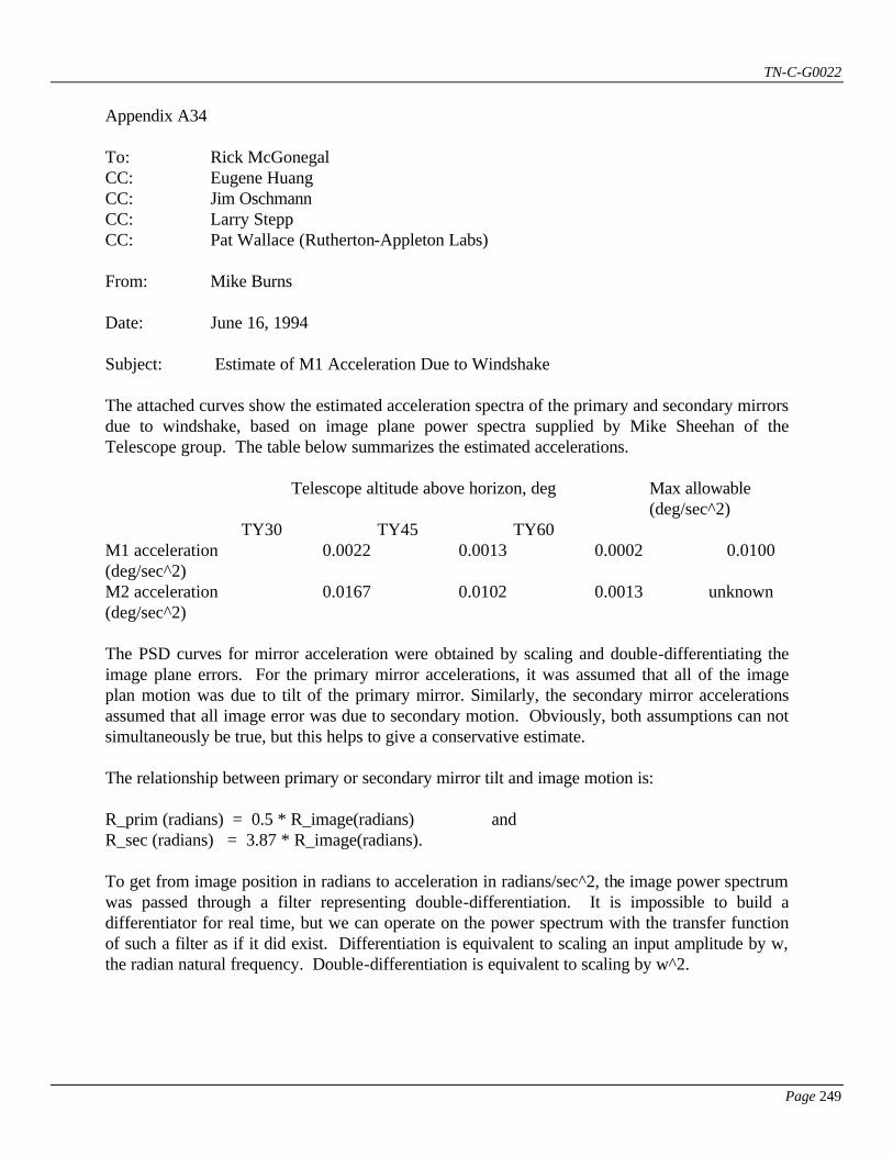
TN-C-G0022

Page 249

Appendix A34 To: Rick McGonegal CC: Eugene Huang CC: Jim Oschmann CC: Larry Stepp CC: Pat Wallace (Rutherton-Appleton Labs) From: Mike Burns Date: June 16, 1994 Subject: Estimate of M1 Acceleration Due to Windshake The attached curves show the estimated acceleration spectra of the primary and secondary mirrors due to windshake, based on image plane power spectra supplied by Mike Sheehan of the Telescope group. The table below summarizes the estimated accelerations. Telescope altitude above horizon, deg Max allowable

(deg/sec^2) TY30 TY45 TY60 M1 acceleration (deg/sec^2)

0.0022 0.0013 0.0002 0.0100

M2 acceleration (deg/sec^2)

0.0167 0.0102 0.0013 unknown

The PSD curves for mirror acceleration were obtained by scaling and double-differentiating the image plane errors. For the primary mirror accelerations, it was assumed that all of the image plan motion was due to tilt of the primary mirror. Similarly, the secondary mirror accelerations assumed that all image error was due to secondary motion. Obviously, both assumptions can not simultaneously be true, but this helps to give a conservative estimate. The relationship between primary or secondary mirror tilt and image motion is: R_prim (radians) = 0.5 * R_image(radians) and R_sec (radians) = 3.87 * R_image(radians). To get from image position in radians to acceleration in radians/sec^2, the image power spectrum was passed through a filter representing double-differentiation. It is impossible to build a differentiator for real time, but we can operate on the power spectrum with the transfer function of such a filter as if it did exist. Differentiation is equivalent to scaling an input amplitude by w, the radian natural frequency. Double-differentiation is equivalent to scaling by w^2.

TN-C-G0022

Page 250

Since the power spectrum represents the square of amplitude, the scale factors described above must be similarly squared. So the relationships between image plane power spectrum and mirror acceleration power spectra are: PSD_M1_accel = PSD_image*(0.5^2)*(w^4) and PSD_M2_accel = PSD_image*(3.87^2)*(w^4). In order to get RMS acceleration, the power spectra must first be integrated over frequency to get net power. Then the square-root of power gives RMS. There is the possibility of considerable error in estimating the RMS of acceleration in this way. The power spectrum should be integrated over all frequencies, not just up to 100Hz. Looking at figure 1, the power spectrum falls off very slowly from 60-100Hz. If it continued to fall off this slowly, the integral up to infinite frequency would be infinite. A log-log plot of power spectrum must fall off with slope less than -1 to be integrable (i.e. we can only integrate 1/x^n if n is greater than 1).

TN-C-G0022

Page 251

Appendix A35 To: Rick McGonegal From: Mike Burns Date: June 15, 1994 Subject: A Slewing Controller for the Gemini Azimuth and Altitude Drives 1 SUMMARY A controller is demonstrated which is capable of slewing the telescope for large angular changes without exceeding the recommended limits on angular velocity or acceleration. The controller smoothly transitions at the appropriate times in order to accelerate maximally, then to hold constant velocity, then decelerate maximally, and finally to apply linear control for tracking. The attached results are for fine encoder resolutions, such as would exist during tracking. Since the encoders degrade at high angular rates, the runs must be repeated for coarser encoder quantization. 2 CONTROLLER DESCRIPTION Figure 1 shows the azimuth controller with inputs of angular position and angle command, and with an output of torque delivered to the mount. The angular position is the difference between the pier rotation (almost zero) and the mount rotation in radians, and is sensed by the resolver. The measured angle and commanded angle are read by the digital controller which generates a commanded motor rate. The commanded motor rate suffers the quantization effect of a DA converter to become a voltage in the analog motor velocity loop, and the motor finally generates torque that is supplied to the telescope mount. Only the azimuth drive is described here, but the altitude drive is organized similarly. Figure 2 shows more detail of the digital controller from figure 1. The commanded and measured positions are combined to form an error signal. This error signal is fed to the switching logic which determines which of three modes the controller should operate in: acceleration, velocity or linear. The linear mode is for tracking and very small angular errors. The acceleration mode is active during large errors, but when the velocity has not yet approached the rate limit. The velocity mode is used to hold constant velocity near the maximum allowable rate, but not exceed the rate limit. The normal operation of slewing, it would be expected to accelerate at the maximum rate for half of the distance then decelerate at the maximum rate for the other half of the slew. For larger slewing angles, say greater than 20 degrees, the maximum velocity would be reached, so there would be no more acceleration until it was time to decelerate.

TN-C-G0022

Page 252

Figure 3 shows the linear controller which is used during tracking. It is effectively a PI (proportional and integral) controller with a velocity feedforward term to match the small velocity of the commanded signal. When the control signal is zero, representing deactivation of the linear control mode, the integral output is initialized to zero to prevent "windup". Figure 4 shows the controller for the constant velocity mode. The commanded rate is the maximum rate (0.035 rad/sec for azimuth) with sign determined by the sign of the error signal. In order to control velocity, it is necessary to have some measure of velocity, so the error signal is passed though a filter which approximates a band-limited differentiator. The available bandwidth of the rate estimator, and therefore the available bandwidth of the velocity controller, is determined by the noise on the error signal. Since the error signal is derived from the angle encoders, coarser encoders would have more noise. The difference between the commanded rate and estimated rate passes through a PI controller and gives the commanded motor rate necessary to maintain constant telescope velocity even under disturbances such as variation in wind and friction. Coarser encoders would force a reduction in bandwidth, which would allow disturbances to have a greater effect on changing the telescope velocity. Figure 5 shows the controller for acceleration mode. It is similar to the velocity mode controller described above, in that there is an estimate of acceleration made, and this is compared to the commanded acceleration (either positive maximum for acceleration, or negative maximum for deceleration) to get an error signal. It was found necessary to use a PII (proportional-integral-integral) controller for acceleration. This was driven by the desire to have a zero steady state acceleration error, i.e. that the achieved acceleration should eventually equal the commanded acceleration. 3 RESULTS Figures 6 through 15 show the results of simulating the proposed slewing controller. Various slewing step sizes are examined ranging from tiny (1 arcminute) to large (90 degrees). The first five runs, figures 6 through 10, are for azimuth and the latter five runs are for altitude movements. Figure 6 shows the response of the azimuth controller for approximately a 1 arcminute step. The upper left plot shows the azimuth position in radians, settles out to the commanded value in less than 2 seconds. The upper right plot shows the error signal which goes to zero as expected. The lower left plot shows the derivative of the error signal. For this small step, the rate signal is far below the azimuth limit of 0.035 rad/sec (2 degrees/sec). The lower right plot shows the acceleration is first near the maximum in one direction then decelerates maximally. The acceleration limit of 1.7e-3 rad/sec^2 (0.1 degrees/sec^2) is approached but not exceeded. Figures 7, 8 and 9 show the responses for azimuth steps of 3 arcminutes, 1 degree and 20 degrees respectively. Each response shows that the velocity and acceleration limits are not exceeded, and the controller eventually settles down to a linear tracking mode within a reasonable amount of time.

TN-C-G0022

Page 253

Figure 10 shows the response for a 90 degree change in azimuth. Note that the velocity limit is approached, representing the flat portion of the velocity curve between 20 and 35 seconds in the lower left plot of Figure 10. The deceleration period, between 35 and 80 seconds, is a bit "choppy". This is due to the difficulty of the controller in estimating the correct time to apply deceleration. The results of the altitude runs, figures 11 through 15, show qualitatively the same behavior as the azimuth runs. The altitude velocity limit of 0.013 rad/sec (0.75 degrees/sec) and the acceleration limit of 5.2e-4 rad/sec^2 (0.03 deg/sec^2) are similarly protected by the controller. 4 FURTHER WORK The described controller was tested subject to encoder resolutions consistent with tracking. It is expected that the encoder resolution will be coarser when the slew rate exceeds about 0.5 deg/sec (0.009 rad/sec). This will cause large noise on the measured angular position, which is expected to force some reduction in the available bandwidth of the acceleration and velocity controllers described. The reduction in bandwidth will cause the controller to take somewhat more time to achieve the maximum acceleration, leading to longer slewing times. Disturbances such as wind gusts and friction variation will not be compensated for as quickly.

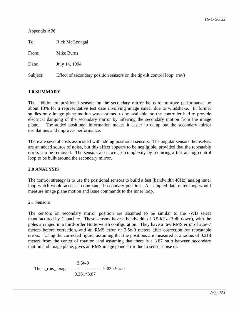
TN-C-G0022

Page 254

Appendix A36 To: Rick McGonegal From: Mike Burns Date: July 14, 1994 Subject: Effect of secondary position sensors on the tip-tilt control loop (rev) 1.0 SUMMARY The addition of positional sensors on the secondary mirror helps to improve performance by about 13% for a representative test case involving image smear due to windshake. In former studies only image plane motion was assumed to be available, so the controller had to provide electrical damping of the secondary mirror by inferring the secondary motion from the image plane. The added positional information makes it easier to damp out the secondary mirror oscillations and improves performance. There are several costs associated with adding positional sensors. The angular sensors themselves are an added source of noise, but this effect appears to be negligible, provided that the repeatable errors can be removed. The sensors also increase complexity by requiring a fast analog control loop to be built around the secondary mirror. 2.0 ANALYSIS The control strategy is to use the positional sensors to build a fast (bandwidth 40Hz) analog inner loop which would accept a commanded secondary position. A sampled-data outer loop would measure image plane motion and issue commands to the inner loop. 2.1 Sensors The sensors on secondary mirror position are assumed to be similar to the -WB series manufactured by Capacitec. These sensors have a bandwidth of 3.5 kHz (3 db down), with the poles arranged in a third-order Butterworth configuration. They have a raw RMS error of 2.5e-7 meters before correction, and an RMS error of 2.5e-9 meters after correction for repeatable errors. Using the corrected figure, assuming that the positions are measured at a radius of 0.318 meters from the center of rotation, and assuming that there is a 3.87 ratio between secondary motion and image plane, gives an RMS image plane error due to sensor noise of: 2.5e-9 Theta_rms_image = ---------------- = 2.03e-9 rad 0.381*3.87

TN-C-G0022

Page 255

The above noise RMS is about a factor of 10 below the image centroiding error and a factor of 100 below the compensated windshake RMS, so it is expected to go unnoticed. The secondary position sensor noise would start to become significant at about 4 times the levels modeled. Under low wind conditions, where image centroiding noise dominates, the secondary position sensor noise would increase the total RMS image error by about 4%. 2.2 Position Inner Loop It is the responsibility of the analog inner loop to accept a commanded secondary mirror position and rapidly drive the mirror to that position, compensating for the dynamic effects of the mirror upon the voice coil actuators. The interaction between the mirror assembly and the telescope top-end are neglected. Figure 1 shows the block diagram of the position inner loop. The controller has 1 pole and 1 zero to provide some phase lead and move the slow, underdamped plant modes (6Hz, 0.03 damping) to more desirable locations (40Hz, 0.9 damping). The denominator of the inner loop compensator is at 350Hz, which is fast compared to the chose inner loop poles yet slow compared to the position sensors (3.5 kHz). The bandwidth of 40Hz on the inner loop was chosen to be considerably below the structural resonance of the telescope top end (around 120Hz), so that the structure could be neglected. If the structural resonances were important, the controller would need to be much more complicated in an attempt to overcome the effect of the phase lag and rapidly changing gain near resonance. Figure 2 shows the response to a commanded step of 1 micro-radian. From a spectral density of wind induced image plane motion, it can be shown that the RMS change in the secondary position for each time step is approximately 0.8 micro-radians, so the 1 micro-radian test is fairly representative. The upper left plot of figure 2 shows the mirror position versus time. The upper right plot shows the error signal, which is 1e-6 minus the position. The lower left plot shows the required current in the actuators. The lower right plot of figure 2 shows the power, based on the current curve and the knowledge that there are 3 actuators each with 2 ohms resistance. Calculating the average power over the first 0.005 seconds gives 0.2mW which is quite small. Earlier estimates showed power consumption of 2mW and included the lower frequency mirror motion. The table below shows the approximate power needed by the secondary inner loop under the design presented here. Power (W) given inner loop bandwidth 40Hz 120Hz 350Hz 1.8e-4 (W) 1.0e-2 (W) 2.3 (W) Table 1: Tip-tilt secondary inner loop power consumption for various inner loop bandwidths. The tilt inner loop bandwidth is probably limited to near 350Hz due to the bandwidth of the position sensors. 2.3 Digital Outer Loop The block diagram for the digital outer loop is shown in figure 3. The position inner loop is embedded in this block diagram in a simplified form as 2 poles at 40Hz. The digital controller is

TN-C-G0022

Page 256

modeled as a PI controller plus a lead-lag as it was in earlier papers. When the filtering functions of figure 4 are applied to a power spectrum representing the TY30 case of windshake, the net RMS image error after tip-tilt correction may be obtained versus sampling rate as shown in figure 5. For the nominal sampling rate of 200Hz, the loop with tilt position sensors shows a 13% improvement over the loop with no sensors, reducing the RMS image centroid error from 0.41 microradians to 0.36 microradians. For sampling rates about 350Hz, the system with tilt sensors becomes inferior to the system lacking such sensors. The reason for this is that the 40Hz inner loop bandwidth starts to limit performance, since the outer loop is trying to accomplish a higher bandwidth. 3.0 FURTHER WORK This work is preliminary and rather unreliable. In order to get a better understanding of the potential benefit of adding tip-tilt sensors to the secondary mirror control loop it would be desirable to include a model of the telescope structure, especially if the inner loop were asked to have a bandwidth above 40Hz. It is known that there will be momentum compensation for the tip-tilt system which should make the telescope appear stiffer to the inner loop controller. The model described above assumes optimistically that the tip-tilt inner loop is reacting against ground. The tip-tilt inner loop bandwidth will likely be limited by the success of the momentum compensation scheme in making the telescope appear stiff. It is not currently known how to model the degradation caused by imperfect momentum compensation.

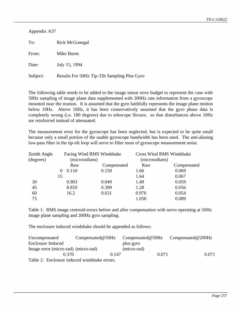
TN-C-G0022

Page 257

Appendix A37 To: Rick McGonegal From: Mike Burns Date: July 15, 1994 Subject: Results For 50Hz Tip-Tilt Sampling Plus Gyro The following table needs to be added to the image smear error budget to represent the case with 50Hz sampling of image plane data supplemented with 200Hz rate information from a gyroscope mounted near the trunion. It is assumed that the gyro faithfully represents the image plane motion below 10Hz. Above 10Hz, it has been conservatively assumed that the gyro phase data is completely wrong (i.e. 180 degrees) due to telescope flexure, so that disturbances above 10Hz are reinforced instead of attenuated. The measurement error for the gyroscope has been neglected, but is expected to be quite small because only a small portion of the usable gyroscope bandwidth has been used. The anti-aliasing low-pass filter in the tip-tilt loop will serve to filter most of gyroscope measurement noise. Zenith Angle (degrees)

Facing Wind RMS Windshake (microradians)

Cross Wind RMS Windshake (microradians)

Raw Compensated Raw Compensated 0 0.110 0.150 1.66 0.069

15 1.64 0.067 30 0.903 0.049 1.49 0.059 45 8.810 0.399 1.28 0.056 60 16.2 0.631 0.976 0.054 75 1.050 0.089 Table 1: RMS image centroid errors before and after compensation with servo operating at 50Hz image plane sampling and 200Hz gyro sampling. The enclosure induced windshake should be appended as follows: Uncompensated Enclosure Induced Image error (micro-rad)

Compensated@50Hz (micro-rad)

Compensated@50Hz plus gyro (micro-rad)

Compensated@200Hz

0.370 0.147 0.071 0.071 Table 2: Enclosure induced windshake errors.

TN-C-G0022

Page 258

In general, the above results with gyros fall somewhere between the performance of the 50Hz system and the 200Hz system without gyros. As a practical matter, we might not want to limit ourselves to having the servo loop operating at 200Hz if a gyro is available. In control systems there is typically a tradeoff between measurement noise and disturbance. A higher bandwidth increases the effect of measurement noise but decreases the disturbance. So a bandwidth is chosen which makes these two sources roughly equal, thus minimizing the RSS. Further work would include modeling the gyroscope noise and choosing a bandwidth accordingly. It would probably be advantageous to have the rate of the tip-tilt loop automatically vary with perceived conditions so that the minimum RSS error was obtained depending on wind, pointing, gyroscope noise and other errors. A lookup table could be built which selected the best sampling rate. The rate should vary slowly, and of course the rate should be over-ridable by the operator. We might also be limited in sampling rate, and therefore bandwidth, by the computer burden imposed by a very fast sampled data system. Even if this is the case, it would still be worth knowing the performance which could be achieved given faster computers.

TN-C-G0022

Page 259

Appendix A38 To: Rick McGonegal (8M) CC: Richard Kurz (8M) CC: Peregrine McGehee (8M) CC: Matt Mountain (8M) CC: Jim Oschmann (8M) CC: David Robertson (8M) CC: Doug Simons (8M) CC: Malcolm Stewart (ROE) CC: Magnus Patterson (ROE) CC: Nick Dillon (RGO) CC: Dave Gellatly (RGO) CC: Charles Jenkins (RGO) CC: Robert Laing (RGO) From: Mike Burns Date: June 8, 1994 Subject: Compensated Windshake Results for Tip-tilt with Integration Delay SUMMARY The effect upon the tip-tilt control loop of various delays is to harm the phase margin and cause a larger RMS tracking error. Three sources of delay are considered: CCD integration time, numerical processing delay, and a sample-and-hold. Results are quoted for varying the numerical processing delay from 0ms to 5ms. A processing delay of 0.5ms is acceptable, but larger delays are probably not. SIMULATION DESCRIPTION Figure 1 shows a block diagram for the simulation used in this memo. The input disturbance, in this case windshake, can be thought of as a commanded angular position for the secondary mirror. It is compared to the actual secondary position, labeled theta, to get a real error signal. The root mean square (RMS) of this error signal over time represents the performance measure of the tip-tilt secondary. The true error signal passes through a delay representing the effect of integration within the charge coupled devices (CCD's) plus some small processing delay. The error signal is then passed to a digital filter with an implied sample-and-hold. In this simulation, the digital filtering is composed of a lead-lag filter and a second-order proportional-integral (PI) controller. The controller commands a torque which acts upon the plant and anti-aliasing filter to produce change theta, the angle of the secondary mirror, thus closing the loop.

TN-C-G0022

Page 260

The plant is modeled as having a moment of inertia of 4 kg-m^2, a natural frequency of around 6.4Hz and light damping of about 3%. The simulation operates in the frequency domain. A transfer function is computed from disturbance in to error out. This transfer function is multiplied by an input power spectrum (rad^2/Hz) to get a power spectrum after compensation. The resulting power spectrum is integrated over frequency, and the square root gives an RMS tracking error in radians. The effect upon the tip-tilt control loop of the various delays is to harm the phase margin which in turn lowers the achievable bandwidth for a given sampling frequency. A lower bandwidth results in the tip-tilt loop removing less of the disturbance and ultimately causes a larger tracking error. Even if a control loop with a poor phase margin seemed to give acceptable performance in the simulation, it would still not be advisable to build such a system. A system with low phase margin is not robust and can be easily made to ring or become unstable. For this analysis, the system was designed for a phase margin of 60 degrees and a gain margin of 3 dB. This is near the edge of what could be considered good control design. Some engineers prefer more generous margins of 70 degrees and 6 dB. There are three sources of delay between the existence of a true tracking error and the application of a correcting torque upon the secondary mirror. The CCD's must integrate the error signal. Since the loop is assumed to operate at 200Hz, the average time delay due to integration is half of a period, or 2.5ms. Next there is the delay associated with numerical processing, which was varied between the nominal value of 0.5ms and an upper limit 5ms for this study. A third source of delay is the required sample and hold after the integrator at the input to the digital filter. The sample-and-hold ads about half of a period, or 2.5ms of delay. Figure 2 shows the effect of the various delay sources. The upper left plot shows an input signal, representing image plane error in microradians for example. The upper right shows the corresponding output from the CCD, modeled as an integrator which is reset at 200Hz and scaled appropriately. The lower left plot shows the effect of a sample and hold and the lower right plot ads a bit more delay to account for the numerical processing. RESULTS Table 1 shows the compensated RMS windshake as a fraction of the error budget for the simulated tip-tilt loop. The error budget includes the effect of direct windshake and indirect windshake through the enclosure, but does not take into account the centroid measuring error, which is expect to be small (i.e. 0.027 microradians) compared to the other terms. The telescope is assumed to be pointed into the wind and the altitude axis is varied from 30 degrees above horizon to 90 degrees (i.e. zenith pointing). The direct effect of wind upon the telescope topend is the dominant source of motion in the image plane, but the indirect effect of wind upon the enclosure has also been included.

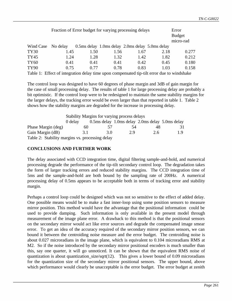
TN-C-G0022

Page 261

Fraction of Error budget for varying processing delays Error Budget micro-rad

Wind Case No delay 0.5ms delay 1.0ms delay 2.0ms delay 5.0ms delay TY30 1.45 1.50 1.56 1.67 2.18 0.277 TY45 1.24 1.28 1.32 1.42 1.82 0.212 TY60 0.41 0.41 0.41 0.42 0.45 0.180 TY90 0.75 0.77 0.78 0.83 1.03 0.158 Table 1: Effect of integration delay time upon compensated tip-tilt error due to windshake The control loop was designed to have 60 degrees of phase margin and 3dB of gain margin for the case of small processing delay. The results of table 1 for large processing delay are probably a bit optimistic. If the control loop were to be redesigned to maintain the same stability margins for the larger delays, the tracking error would be even larger than that reported in table 1. Table 2 shows how the stability margins are degraded for the increase in processing delay. Stability Margins for varying process delays 0 delay 0.5ms delay 1.0ms delay 2.0ms delay 5.0ms delay Phase Margin (deg) 60 57 54 48 31 Gain Margin (dB) 3.1 3.0 2.9 2.6 1.9 Table 2: Stability margins vs. processing delay CONCLUSIONS AND FURTHER WORK The delay associated with CCD integration time, digital filtering sample-and-hold, and numerical processing degrade the performance of the tip-tilt secondary control loop. The degradation takes the form of larger tracking errors and reduced stability margins. The CCD integration time of 5ms and the sample-and-hold are both bound by the sampling rate of 200Hz. A numerical processing delay of 0.5ms appears to be acceptable both in terms of tracking error and stability margin. Perhaps a control loop could be designed which was not so sensitive to the effect of added delay. One possible means would be to make a fast inner-loop using some position sensors to measure mirror position. This method would have the advantage that the positional information could be used to provide damping. Such information is only available in the present model through measurement of the image plane error. A drawback to this method is that the positional sensors on the secondary mirror would act like error sources and degrade the compensated image smear error. To get an idea of the accuracy required of the secondary mirror position sensors, we can bound it between the centroiding noise measure and the error budget. The centroiding noise is about 0.027 microradians in the image plane, which is equivalent to 0.104 microradians RMS at M2. So if the noise introduced by the secondary mirror positional encoders is much smaller than this, say one quarter, it will go unnoticed. It can be shown that the equivalent RMS noise of quantization is about quantization_size/sqrt(12). This gives a lower bound of 0.09 microradians for the quantization size of the secondary mirror positional sensors. The upper bound, above which performance would clearly be unacceptable is the error budget. The error budget at zenith

TN-C-G0022

Page 262

is 0.158 microradians RMS in the image plane, or 0.61 microradians motion of M2. This leads to an acceptable quantization step size of 0.61*sqrt(12)=2.1 microradians. So it would seem that if the secondary mirror position sensors had smaller error than 0.09 microradians, they would go unnoticed, and if they had a larger error than 2.1 microradians the results would be guaranteed to be unacceptable. In the region between 0.09 and 2.1 microradians, further study would be required to quantify the tradeoff between better damping and the increased noise due to positional measurement error. Another possible method would be to use fiber optic gyros (FOG's) to obtain high frequency windshake motion, and lower the required sampling rate. A complimentary filter would be implemented to blend the high-frequency information from the FOG with low frequency information from the wavefront sensor. A lower sampling rate results in proportionately less phase margin degradation for a given delay time.

Documents

GEMINI 8-M TELESCOPES PROJECT · Study", Systems Technology ... Thompson, P. Phd, "Keck Telescope Elevation AxisServo Design Evaluation and Feasibility Study", ... for a baseline