Geir Evensen

The Ensemble Kalman Filter: theoretical formulationand practical implementation

Received: 16 December 2002 /Accepted: 7 May 2003! Springer-Verlag 2003

Abstract The purpose of this paper is to provide acomprehensive presentation and interpretation of theEnsemble Kalman Filter (EnKF) and its numericalimplementation. The EnKF has a large user group,and numerous publications have discussed applicationsand theoretical aspects of it. This paper reviews theimportant results from these studies and also presentsnew ideas and alternative interpretations which furtherexplain the success of the EnKF. In addition to pro-viding the theoretical framework needed for using theEnKF, there is also a focus on the algorithmic for-mulation and optimal numerical implementation. Aprogram listing is given for some of the key subrou-tines. The paper also touches upon specific issues suchas the use of nonlinear measurements, in situ profilesof temperature and salinity, and data which areavailable with high frequency in time. An ensem-ble based optimal interpolation (EnOI) scheme ispresented as a cost-e!ective approach which may serveas an alternative to the EnKF in some applications. Afairly extensive discussion is devoted to the use of timecorrelated model errors and the estimation of modelbias.

Keywords Data assimilation ! Ensemble Kalman Filter

1 Introduction

The Ensemble Kalman Filter has been examined andapplied in a number of studies since it was first intro-duced by Evensen (1994b). It has gained popularitybecause of its simple conceptual formulation and rela-

tive ease of implementation, e.g., it requires no deriva-tion of a tangent linear operator or adjoint equations,and no integrations backward in time. Further, thecomputational requirements are a!ordable and compa-rable with other popular sophisticated assimilationmethods such as the representer method by Bennett(1992); Bennett et al. (1993, 1996); Bennett and Chua(1994) and the 4DVAR method which has been muchstudied by the meteorological community (see, e.g.,Talagrand and Courtier 1997, 1987; Courtier andTalagrand 1987; Courtier et al. 1994).

This paper gives a comprehensive presentation ofthe Ensemble Kalman Filter (EnKF), and it may serveas an EnKF reference document. For a user of theEnKF it provides citations from hopefully all previouspublications where the EnKF has been examined orused. It also provides a detailed presentation of themethod in terms of both theoretical aspects and practicalimplementation. For experienced EnKF users it willprovide a better understanding of the EnKF through thepresentation of a new and alternative interpretation andimplementation of the analysis scheme.

In the next section, an overview is given of previousworks involving the EnKF. Further, in Section 3, anoverview of the theoretical formulation of the EnKF willbe given. Thereafter the focus will be on implementationissues, starting with the generation of the initial ensem-ble in Section 4.1 and the stochastic integration of theensemble members in Section 4.2. The major discussionin this paper relates to the EnKF analysis scheme, whichis given in Section 4.3. Section 5 discusses particularaspects of the numerical implementation. Appendix Apresents an approach for examining the consistency ofthe EnKF based on comparisons of innovations andpredicted error statistics. In Appendix B an optimalinterpolation algorithm is presented. It uses a stationaryensemble but is otherwise similar to the EnKF, and itcan thus be denoted Ensemble Optimal Interpolation(EnOI). In Appendix C we have given an algorithmwhich is currently used for assimilation of observationsof subsurface quantities. In Appendix D the Ensemble

Ocean Dynamics (2003) 53: 343–367DOI 10.1007/s10236-003-0036-9

Responsible Editor: Jorg-Olaf Wol!

Geir EvensenNansen Environmental and Remote Sensing Center,Bergen Norway Edvard Griegsvei 3A,5059 Solheimsviken, Norwaye-mail: Geir.Evensen@nersc.no

Kalman Smoother (EnKS) is presented in terms of theterminology developed in this paper. It is illustrated howthe smoother solution can be very e"ciently computedas a reanalysis following the use of the EnKF. InAppendix E we have reviewed and detailed the presen-tation of the algorithm used for the generation ofpseudorandom fields. Finally, in Appendix F an exam-ple is given illustrating the EnKF and EnKS with asimple stochastic scalar model. This illustrates the use oftime-correlated model errors and how these can beestimated. The use of the EnKF and EnKS for estima-tion of model bias is given in Appendix G.

2 Chronology of ensemble assimilation developments

This section attempts to provide a complete overview ofthe developments and applications related to the EnKF.In addition, it also points to other recently proposedensemble-based methods and some smoother applica-tions.

2.1 Applications of the EnKF

Applications involving the EnKF are numerous andinclude the initial work by Evensen (1994b) and anadditional example in Evensen (1994a), which showedthat the EnKF resolved the closure problems reportedfrom applications of the Extended Kalman Filter(EKF).

An application with assimilation of altimeter data forthe Agulhas region was discussed in Evensen and vanLeeuwen (1996) and later in a comparison with theEnsemble Smoother (ES) by van Leeuwen and Evensen(1996).

An example with the Lorenz equations was presentedby Evensen (1997), where it was shown that the EnKFcould track the phase transitions and find a consistentsolution with realistic error estimates even for such achaotic and nonlinear model.

Burgers et al. (1998) reviewed and clarified somepoints related to the perturbation of measurements inthe analysis scheme, and also gave a nice interpretationsupporting the use of the ensemble mean as the bestestimate.

Houtekamer and Mitchell (1998) introduced a vari-ant of the EnKF where two ensembles of model statesare integrated forward in time, and statistics from oneensemble are used to update the other. The use of twoensembles was motivated by claiming that this wouldreduce possible inbreeding in the analysis. This has,however, led to some dispute, discussed in the commentby van Leeuwen (1999a) and the reply by Houtekamerand Mitchell (1999).

Miller et al. (1999) included the EnKF in a compar-ison with nonlinear filters and the Extended KalmanFilter, and concluded that it performed well, but couldbe beaten by a nonlinear and more expensive filter in

di"cult cases where the ensemble mean is not a goodestimator.

Madsen and Canizares (1999) compared the EnKFand the reduced rank square root implementation of theExtended Kalman filter with a 2-D storm surge model.This is a weakly nonlinear problem, and good agreementwas found between the EnKF and the extended Kalmanfilter implementation.

Echevin et al. (2000) studied the EnKF with a coastalversion of the Princeton Ocean Model and focused inparticular on the horizontal and vertical structure ofmultivariate covariance functions from sea-surfaceheight. It was concluded that the EnKF could captureanisotropic covariance functions resulting from the im-pact of coastlines and coastal dynamics, and had aparticular advantage over simpler methodologies in suchareas.

Evensen and van Leeuwen (2000) rederived theEnKF as a suboptimal solver for the general Bayesianproblem of finding the posterior distribution givendensities for the model prediction and the observations.From this formulation the general filter, could bederived and the EnKF could be shown to be a subop-timal solver of the general filter, where the prior densitiesare assumed to be Gaussian distributed.

Hamill and Snyder (2000) constructed a hybridassimilation scheme by combining 3DVAR and theEnKF. The estimate is computed using the 3DVARalgorithm but the background covariance is a weightedaverage of the time evolving EnKF error covariance andthe constant 3DVAR error covariance. A conclusionwas that with increasing ensemble size the best resultswere found with larger weight on the EnKF errorcovariance.

Hamill et al. (2000) report from working groups in aworkshop on ensemble methods.

Keppenne (2000) implemented the EnKF with a two-layer shallow-water model and examined the method intwin experiments assimilating synthetic altimetry data.He focused on the numerical implementation on parallelcomputers with distributed memory, and found the ap-proach e"cient for such systems. He also examined theimpact of ensemble size and concluded that realisticsolutions could be found using a modest ensemble size.

Mitchell and Houtekamer (2000) introduced anadaptive formulation of the EnKF, where the model er-ror parameterization was updated by incorporatinginformation from the innovations during the integration.

Park and Kaneko (2000) presented an experimentwhere the EnKF was used to assimilate acoustictomography data into a barotropic ocean model.

van Loon et al. (2000) used the EnKF for assimila-tion of ozone data into an atmospheric transportchemistry model.

Grønnevik and Evensen (2001) examined the EnKFfor use in fish stock assessment, and also compared itwith the Ensemble Smoother (ES) by van Leeuwen andEvensen (1996) and the more recent Ensemble KalmanSmoother (EnKS) by Evensen and van Leeuwen (2000).

344

Heemink et al. (2001) have been examining di!erentapproaches which combine ideas from RRSQRT filter-ing and the EnKF to derive computationally more e"-cient methods.

Houtekamer and Mitchell (2001) have continued theexamination of the two-ensemble approach and intro-duced a technique for computing the global EnKFanalysis in the case with many observations, and also amethod for filtering of eventual long range spuriouscorrelations caused by a limited ensemble size. As will beseen below, the current paper presents a much moree"cient way to compute the global analysis and alsoargues against filtering of covariances.

Pham (2001) reexamined the EnKF in an applicationwith the Lorenz attractor and compared results withthose obtained from di!erent versions of the SingularEvolutive Extended Kalman (SEEK) filter and a particlefilter. Ensembles with very few members were usedand this favored methods like the SEEK where the‘‘ensemble’’ of EOFs is selected as a best-possible rep-resentation of the model attractor.

Verlaan and Heemink (2001) applied the RRSQRTand EnKF filters in test examples with the purpose ofclassifying and defining a measure of the degree ofnonlinearity of the model dynamics. Such an estimatemay have an impact on the choice of assimilationmethod.

Hansen and Smith (2001) proposed a method forproducing analysis ensembles based on integrated use ofthe 4DVAR method and the EnKF. A probabilisticapproach was used and lead to high numerical cost, butan improved estimate could be found compared to4DVAR and the EnKF used separately.

Hamill et al. (2001) examined the impact of ensemblesize on noise in distant covariances. They evaluated theimpact of using an inflation factor, as introduced byAnderson and Anderson (1999), and also the use of aSchur product of the covariance with a correlationfunction to localize the background covariances, aspreviously discussed by Mitchell (2001). The inflationfactor is used to replace the forecast ensemble accordingto:

wj " q#wj $ !ww% & !ww; #1%

with q slightly greater than 1 (typically 1.01). The pur-pose is to account for a slight underrepresentation ofvariance due to the use of a small ensemble.

Bishop et al. (2001) used an implementation of theEnKF in an observation system simulation experiment.Ensemble-predicted error statistics were used to deter-mine the optimal configuration of future targetedobservations. The application typically looked at a casewhere additional targeted measurements could be de-ployed over the next few days and the deployment couldbe optimized to minimize the forecast errors in a selectedregion. The methodology was named Ensemble Trans-form Kalman Filter and it was further examined byMajumdar et al. (2001).

Reichle et al. (2002) give a nice discussion of theEnKF in relation to the optimal representer solution.They find good convergence of the EnKF toward therepresenter solution, with the di!erence being caused bythe Gaussian assumptions used in the EnKF at analysissteps. These are avoided in the representer method,which solves for the maximum-likelihood smootherestimate.

Bertino et al. (2002) applied the EnKF and the Re-duced Rank Square Root (RRSQRT) filter with a modelfor the Odra estuary. The two methods were comparedand used to assimilate real observations to assess thepotential for operational forecasting in the lagoon. Thisis a relatively linear model and the EnKF and theRRSQRT filter provided similar results.

Eknes and Evensen (2002) examined the EnKF with a1-D three component marine ecosystem model with fo-cus on sensitivity to the characteristics of the assimilatedmeasurements and the ensemble size. It was found thatthe EnKF could handle strong nonlinearities andinstabilities which occur during the spring bloom.

Allen et al. (2002) take the Eknes and Evensen (2002)work one step further by applying the method with a 1-D version of ERSEM for a site in the MediterraneanSea. They showed that even with such a complex modelit is possible to find an improved estimate by assimilat-ing in situ data into the model.

Haugen and Evensen (2002) applied the EnKF toassimilate sea-level anomalies and sea-surface tempera-ture data into a version of the Miami Isopycnic Coor-dinate Ocean Model (MICOM) by Bleck et al. (1992)for the Indian Ocean. The paper provided an analysis ofregionally dependent covariance functions in the tropicsand subtropics and also the multivariate impact ofassimilating satellite observations.

Mitchell et al. (2002) examined the EnKF with aglobal atmospheric general circulation model with sim-ulated data resembling realistic operational observa-tions. They assimilated 80 000 observations a day. Thesystem was examined with respect to required ensemblesize, and the e!ect of localization (local analysis at agrid point using only nearby measurements). It wasfound that severe localization could lead to imbalance,but with large enough ratio of influence for themeasurements, this was not a problem, and no digitalfiltering was required. In the experiments they also in-cluded model errors and demonstrated the importanceof this to avoid filter divergence. This work is a signi-ficant step forward and it shows promising results withrespect to using the EnKF with atmospheric forecastmodels.

Crow and Wood (2003) demonstrated that the EnKFis an e!ective and a computationally competitive strat-egy for the assimilation of remotely sensed brightnesstemperature measurements into land-surface models.

Brusdal et al. (2003) discussed a similar applicationto Haugen et al. (2002), but focused on the NorthAtlantic. In addition, this paper included an extensivecomparison of the theoretical background of the EnKF,

345

EnKS, and the SEEK filter, and also compared resultsfrom these methods.

Natvik and Evensen (2003a,b) presented the firstrealistic 3-D application of the EnKF with a marineecosystem model. These papers proved the feasibility ofassimilating SeaWiFS ocean color data to control theevolution of a marine ecosystem model. In addition,several diagnostic methods were introduced which canbe used to examine the statistical and other properties ofthe ensemble.

Keppenne and Rienecker (2003) implemented amassively parallel version of the EnKF with the Posei-don isopycnic coordinate ocean model for the tropicalPacific. They demonstrated the assimilation of in situobservations and focused on the parallelization of themodel and analysis scheme for computers with distrib-uted memory. They also showed that regionalization ofbackground covariances has negligible impact on thequality of the analysis.

Several of the most recent publications cited abovehave proved the feasibility of the ensemble-basedmethods for real oceanographic problems.

2.2 Other ensemble-based filters

The EnKF can also be related to some other sequentialfilters such as the Singular Evolutive Extended Kalman(SEEK) filter by Pham et al. (1998), Brasseur et al.(1999), Carmillet et al. (2001) (see also Brusdal et al.2003, for a comparison of the SEEK and the EnKF);the Reduced Rank Square Root (RRSQRT) filter byVerlaan and Heemink (2001); and the Error SubspaceStatistical Estimation (ESSE) by Lermusiaux and Rob-insin (1999a,b) and Lermusiaux (2001), which can beinterpreted as an EnKF where the analysis is computedin the space spanned by the EOFs of the ensemble.

Anderson (2001) proposed a method denoted theEnsemble Adjustment Kalman Filter, where the analysisis computed without adding perturbations to theobservations. If observations are not perturbed in theEnKF this still gives the correct mean of the analyzedensemble, but results in a too low variance, as explainedby Burgers et al. (1998). This is accounted for in theEAKF by deriving a linear operator which replaces thetraditional gain matrix and results in an updatedensemble which is consistent with theory. A drawbackmay be the required inversion of the measurement errorcovariance when this is nondiagonal. This method be-comes a variant of the square root algorithm used byBishop et al. (2001). It is demonstrated that for smallensembles (10–20 members) the EAKF performs betterthan the EnKF.

Whitaker and Hamill (2002) proposed another ver-sion of the EnKF where the perturbation of observa-tions are avoided. The scheme provides a better estimateof the analysis variance by avoiding the sampling errorsof the observation perturbations. The scheme was testedfor small ensemble sizes (10–20 members), where it had a

clear benefit on the results when compared to the EnKF,which has larger sampling errors with such smallensemble sizes. The scheme is based on a redefinition ofthe Kalman gain derived from the equation

Pae " #I$ KH%Pf #I$HTKT % & KRKT

" #I$ KH%Pf ; #2%

where the term KRKT " 0 without perturbations ofmeasurements. A solution of this equation is:

K " PfHT!!!!!!!!!!!!!!!!!!!!!!!!!!HPfHT & R

p" #$1$ %T

'!!!!!!!!!!!!!!!!!!!!!!!!!!HPfHT & R

p&

!!!!Rph i$1

: #3%

An explanation of the terms in these equations is givenin Section 3. This is essentially a Monte Carlo imple-mentation of the square root filter and was namedEnSRF.

A summary of the square root filters by Bishop et al.(2001), Anderson (2001), and Whitaker and Hamill(2002) has been given by Tippet et al. (2003), and seealso the general discussion of ensemble methods in a‘‘local least-squares framework’’ given by Anderson(2003).

2.3 Ensemble smoothers

Some publications have focused on the extension of theEnKF to a smoother formulation. The first formulationwas given by van Leeuwen and Evensen (1996), whointroduced the Ensemble Smoother (ES). This methodwas later examined in Evensen (1997) with the Lorenzattractor; applied with a QG model to find a steadymean flow by van Leeuwen (1999b) and for the time-dependent problem in van Leeuwen (2001); and for fishstock assessment by Grønnevik and Evensen (2001).Evensen and van Leeuwen (2000) reexamined thesmoother formulation and derived a new algorithm withbetter properties named the Ensemble KalmanSmoother (EnKS). This method has also been examinedin Grønnevik and Evensen (2001) and Brusdal et al.(2003).

2.4 Nonlinear filters and smoothers

Another extension of the EnKF relates to the derivationof an e"cient method for solving the nonlinear filteringproblem, i.e., taking non-Gaussian contributions in thepredicted error statistics into account when computingthe analysis. These are discarded in the EnKF (seeEvensen and van Leeuwen, 2000), and a fully nonlinearfilter is expected to improve the results when used withnonlinear dynamical models with multi-modal behaviorwhere the predicted error statistics are far from Gauss-ian. Implementations of nonlinear filters based on eitherkernel approximation or particle interpretations have

346

been proposed by Miller et al. (1999), Anderson andAnderson (1999), Pham (2001), Miller and Ehret (2002),and van Leeuwen (2003), although more research isneeded before these can claimed to be practical forrealistic high-dimensional systems.

3 Sequential data assimilation

This section gives a brief introduction to sequential dataassimilation methodologies such as the Kalman Filter(KF) and the Extended Kalman Filter (EKF) and out-lines the general theory of the EnKF.

3.1 A variance-minimizing analysis

The Kalman Filter is a sequential filter method, whichmeans that the model is integrated forward in time and,whenever measurements are available, these are used toreinitialize the model before the integration continues.We neglect the time index and denote a model forecastand analysis as wf and wa, respectively, and the mea-surements are contained in d. Further, the respectivecovariances for model forecast, analysis and measure-ments are denoted Pf , Pa and R. The analysis equationis then:

wa " wf & PfHT #HPfHT & R%$1#d$Hwf %; #4%

with the analysis error covariances given as

Pa " Pf $ PfHT #HPfHT & R%$1HPf : #5%Here H is the measurement operator relating the truemodel state wt to the observations d allowing for mea-surement errors !, i.e.

d " Hwt & !: #6%

The reinitialization, wa, is determined as a weightedlinear combination of the model prediction, wf , andcovariances, PfHT , corresponding to each of the mea-surements in d. The weights are determined by the errorcovariance for the model prediction projected onto themeasurements, the measurement error covariance, andthe di!erence between the prediction and measurements(i.e., the innovation).

The error covariances for the measurements, R, needto be prescribed based on our best knowledge about theaccuracy of the measurements and the methodologiesused to collect them. The error covariances for themodel prediction are computed by solving an equationfor the time evolution of the error covariance matrix ofthe model state.

A derivation of these equations can be found inseveral publications (see, e.g., Burgers et al. 1998). Notethat these equations are often expressed using theso-called Kalman gain matrix

K " PfHT #HPfHT & R%$1: #7%

3.2 The Kalman Filter

Given a linear dynamical model written on discrete formas:

wk&1 " Fwk; #8%the error covariance equation becomes

Pk&1 " FPkFT &Q; #9%

where the matrix Q is the error covariance matrix for themodel errors. The model is assumed to contain errors,e.g., due to neglected physics and numerical approxima-tions. The Eqs. (8) and (9) are integrated to produce theforecasts wf and Pf , used in the analysis Eqs. (4) and (5).

3.3 The Extended Kalman Filter

With a nonlinear model

wk&1 " f#wk%; #10%the error covariance equation is still Eq. (9) but with Fbeing the tangent linear operator (Jacobian) of f#w%.Thus, in the Extended Kalman Filter (EKF), a linearizedand approximate equation is used for the prediction oferror statistics.

3.4 The Ensemble Kalman Filter

The ensemble Kalman filter as proposed by Evensen(1994b) and later clarified by Burgers et al. (1998) is nowintroduced. We will adapt a three-stage presentationstarting with the representation of error statistics usingan ensemble of model states, then an alternative to thetraditional error covariance equation is proposed for theprediction of error statistics, and finally a consistentanalysis scheme is presented.

3.4.1 Representation of error statistics

The error covariance matrices for the forecast and theanalyzed estimate, Pf and Pa, are defined in the Kalmanfilter in terms of the true state as

Pf " #wf $ wt%#wf $ wt%T ; #11%

Pa " #wa $ wt%#wa $ wt%T ; #12%

where the overline denotes an expectation value, w is themodel state vector at a particular time and the super-scripts f , a, and t represent forecast, analyzed, and truestate, respectively. However, the true state is not known,and we therefore define the ensemble covariance matri-ces around the ensemble mean, !ww,

Pf ’ Pfe " #w

f $ wf %#wf $ w

f %T ; #13%

Pa ’ Pae " #w

a $ wa%#wa $ w

a%T ; #14%

347

where now the overlines denote an average over theensemble. Thus, we can use an interpretation where theensemble mean is the best estimate and the spreadingof the ensemble around the mean is a natural definitionof the error in the ensemble mean.

Since the error covariances as defined in Eqs. (13)and (14) are defined as ensemble averages, there willclearly exist infinitively many ensembles with an errorcovariance equal to Pf

e and Pae . Thus, instead of

storing a full covariance matrix, we can represent thesame error statistics using an appropriate ensemble ofmodel states. Given an error covariance matrix, anensemble of finite size will always provide an approx-imation to the error covariance matrix. However, whenthe size of the ensemble N increases, the errors in theMonte Carlo sampling will decrease proportional to1=

!!!!Np

.Suppose now that we have N model states in the

ensemble, each of dimension n. Each of these modelstates can be represented as a single point in an n-dimensional state space. All the ensemble members to-gether will constitute a cloud of points in the state space.Such a cloud of points in the state space can, in the limitwhen N goes to infinity, be described using a probabilitydensity function

/#w% " dNN; #15%

where dN is the number of points in a small unit volumeand N is the total number of points. With knowledgeabout either / or the ensemble representing /, we cancalculate whichever statistical moments (such as mean,covariances, etc.) we want whenever they are needed.

The conclusion so far is that the information con-tained by a full probability density function can be ex-actly represented by an infinite ensemble of model states.

3.4.2 Prediction of error statistics

The EnKF was designed to resolve two major problemsrelated to the use of the EKF with nonlinear dynamics inlarge state spaces. The first problem relates to the use ofan approximate closure scheme in the EKF, and theother to the huge computational requirements associ-ated with the storage and forward integration of theerror covariance matrix.

The EKF applies a closure scheme where third- andhigher-order moments in the error covariance equationare discarded. This linearization has been shown to beinvalid in a number of applications, e.g., Evensen (1992)and Miller et al. (1994). In fact, the equation is no longerthe fundamental equation for the error evolution whenthe dynamical model is nonlinear. In Evensen (1994b) itwas shown that a Monte Carlo method can be used tosolve an equation for the time evolution of the proba-bility density of the model state, as an alternative tousing the approximate error covariance equation in theEKF.

For a nonlinear model where we appreciate that themodel is not perfect and contains model errors, we canwrite it as a stochastic di!erential equation (on contin-uous form) as:

dw " f#w%dt & g#w%dq: #16%

This equation states that an increment in time will yieldan increment in w, which in addition, is influenced by arandom contribution from the stochastic forcing term,g#w%dq, representing the model errors. The dq describe avector Brownian motion process with covariance Qdt.Because the model is nonlinear, g is not an explicitfunction of the random variable dq, so the Ito inter-pretation of the stochastic di!erential equation has to beused instead of the Stratonovich interpretation (seeJazwinski 1970)

When additive Gaussian model errors forming aMarkov process are used, one can derive the Fokker–Planck equation (also named Kolmogorov’s equation)which describes the time evolution of the probabilitydensity /#w% of the model state,

o/ot&X

i

o#fi/%owi

" 1

2

X

i;j

@2/#gQgT %ijowiowj

; #17%

where fi is the component number i of the model oper-ator f and gQgT is the covariance matrix for the modelerrors.

This equation does not apply any importantapproximations and can be considered as the funda-mental equation for the time evolution of error statistics.A detailed derivation is given in Jazwinsky (1970). Theequation describes the change of the probability densityin a local ‘‘volume’’ which is dependent on the diver-gence term describing a probability flux into the local‘‘volume’’ (impact of the dynamical equation) and thedi!usion term which tends to flatten the probabilitydensity due to the e!ect of stochastic model errors. IfEq. (17) could be solved for the probability densityfunction, it would be possible to calculate statisticalmoments like the mean state and the error covariancefor the model forecast to be used in the analysis scheme.

The EnKF applies a so-called Markov Chain MonteCarlo (MCMC) method to solve Eq (17). The proba-bility density can be represented using a large ensembleof model states. By integrating these model states for-ward in time according to the model dynamics describedby the stochastic di!erential Eq. (16), this ensembleprediction is equivalent to solving the Fokker–Planckequation using an MCMC method. This procedureforms the backbone for the EnKF.

A linear model for a Gauss–Markov process in whichthe initial condition is assumed to be taken from anormal distribution will have a probability densitywhich is completely characterized by its mean andcovariance for all times. One can then derive exactequations for the evolution of the mean and thecovariance as a simpler alternative than solving the fullKolmogorov’s equation. Suchmoments ofKolmogorov’s

348

equation, including the error covariance Eq. (9), areeasy to derive, and several methods are illustrated byJazwinski (1970, examples 4.19–4.21). This is actuallywhat is done in the KF and EKF.

For a nonlinear model, the mean and covariancematrix will not in general characterize /#w; t%. They do,however, determine the mean path and the dispersionabout that path, and it is possible to solve approximateequations for the moments, which is the procedurecharacterizing the extended Kalman filter.

An alternative to the approximate stochastic dynamicapproach for solving Kolmogorov’s equation and pre-dicting the error statistics is to use Monte Carlo meth-ods. A large cloud of model states (points in state space)can be used to represent a specific probability densityfunction. By integrating such an ensemble of statesforward in time, it is easy to calculate approximateestimates for moments of the probability density func-tion at di!erent time levels. In this context the MonteCarlo method might be considered a particle method inthe state space.

3.4.3 An analysis scheme

The KF analysis scheme is using the definitions of Pf

and Pa as given by Eqs. (11) and (12). We will now givea derivation of the analysis scheme where the ensemblecovariances are used as defined by Eqs. (13) and (14).This is convenient, since in practical implementationsone is doing exactly this, and it will also lead to a con-sistent formulation of the EnKF.

As will be shown later, it is essential that the obser-vations are treated as random variables having a distri-bution with mean equal to the first-guess observationsand covariance equal to R. Thus, we start by defining anensemble of observations

dj " d& !j; #18%where j counts from 1 to the number of model stateensemble members N . It is ensured that the simulatedrandom measurement errors have mean equal to zero.Next, we define the ensemble covariance matrix of themeasurements as

Re " !!T ; #19%and, of course, in the limit of an infinite ensemblethis matrix will converge toward the prescribed errorcovariance matrix R used in the standard Kalmanfilter.

The following discussion is valid both using an ex-actly prescribed R and an ensemble representation Re ofR. The use of Re introduces an additional approxima-tion which becomes convenient when implementing theanalysis scheme. This can be justified by the fact that theactual observation error covariance matrix is poorlyknown and the errors introduced by the ensemble rep-resentation can be made less than the initial uncertaintyin the exact form of R by choosing a large enough

ensemble size. Further, the errors introduced by using anensemble representation for R have less impact than theuse of an ensemble representation for P. R only appearsin the computation of the coe"cients for the influencefunctions PfHT while P both appears in the computa-tion of the coe"cients and determines the influencefunctions.

The analysis step for the EnKF consists of the fol-lowing updates performed on each of the model stateensemble members

waj " wf

j & PfeH

T #HPfeH

T & Re%$1#dj $Hwfj %: #20%

With a finite ensemble size, this equation will be anapproximation. Further, if the number of measurementsis larger than the number of ensemble members, thematrices HPf

eHT and Re will be singular, and a pseudo

inversion must be used. Note that Eq. (20) implies that

wa " wf & PfeH

T #HPfeH

T & Re%$1#d$Hwf %; #21%where d " d is the first guess vector of measurements.Thus, the relation between the analyzed and forecastensemble mean is identical to the relation between theanalyzed and forecasted state in the standard Kalmanfilter in Eq. (4), apart from the use of Pf ;a

e and Re insteadof Pf ;a and R. Note that the introduction of an ensembleof observations does not make any di!erence for theupdate of the ensemble mean, since this does not a!ectEq. (21).

If the mean, wa, is considered to be the best estimate,then it is an arbitrary choice whether one updates themean using the first-guess observations d, or if one up-dates each of the ensemble members using the perturbedobservations (Eq. 18). However, it will now be shownthat by updating each of the ensemble members usingthe perturbed observations, one also creates a newensemble having the correct error statistics for theanalysis. The updated ensemble can then be integratedforward in time till the next observation time.

Moreover, the error covariance, Pae , of the analyzed

ensemble is reduced in the same way as in the standardKalman Filter. We now derive the analyzed errorcovariance estimate resulting from the analysis schemegiven above, but using the standard Kalman filter formfor the analysis equations. First, note that Eqs. (20) and(21) are used to obtain:

waj $ wa " #I$ KeH%#wf

j $ wf % & Ke#dj $ d%; #22%

where we have used the definition of the Kalman gain,

Ke " PfeH

T #HPfeH

T & Re%$1: #23%

The derivation is then as follows,

Pae " #w

a $ wa%#wa $ wa%T

" #I$ KeH%Pfe #I$HTKT

e % & KeReKTe

" Pfe $ KeHPf

e $ PfeH

TKTe & Ke#HPf

eHT & Re%KT

e

" #I$ KeH%Pfe : #24%

349

The last expression in this equation is the traditionalresult for the minimum variance error covariance foundin the KF analysis scheme. This implies that the EnKFin the limit of an infinite ensemble size will give exactlythe same result in the computation of the analysis asthe KF and EKF. Note that this derivation clearlystates that the observations d must be treated as ran-dom variables to obtain the measurement errorcovariance matrix Re into the expression. It has beenassumed that the distributions used to generate themodel state ensemble and the observation ensemble areindependent.

3.4.4 Summary

We now have a complete system of equations whichconstitutes the ensemble Kalman filter (EnKF), and theresemblance with the standard Kalman filter is main-tained. This is also true for the forecast step. Eachensemble member evolves in time according to the modeldynamics. The ensemble covariance matrix of the errorsin the model equations, given by

Qe " dqkdqTk ; #25%

converges to Q in the limit of infinite ensemble size. Theensemble mean then evolves according to the equation

wk&1 " f#wk%" f#wk% & n.l.; #26%

where n.l. represents the terms which may arise if f isnon-linear. One of the advantages of the EnKF is thatthe e!ect of these terms is retained, since each ensemblemember is integrated independently by the model.

The error covariance of the ensemble evolvesaccording to

Pk&1e " FPk

eFT &Qe & n.l.; #27%

where F is the tangent linear operator evaluated at thecurrent time step. This is again an equation of the sameform as is used in the standard Kalman filter, except ofthe extra terms n.l. that may appear if f is nonlinear.Implicitly, the EnKF retains these terms also for theerror covariance evolution.

For a linear dynamical model, the sampled Pe con-verges to P for infinite ensemble sizes and, independentfrom the model, Re converges to R and Qe converges toQ. Thus, in this limit, both algorithms, the KF and theEnKF, are equivalent.

For nonlinear dynamics the so-called extended Kal-man filter may be used and is given by the evolutionEqs. (26) and (27) with the n.l. terms neglected.Ensemble-based filters include the full e!ect of theseterms and there are no linearizations or closureassumptions applied. In addition, there is no need for atangent linear operator, such as F, or its adjoint, and thismakes these methods very easy to implement for prac-tical applications.

This leads to an interpretation of the EnKF as apurely statistical Monte Carlo method where theensemble of model states evolves in state space withthe mean as the best estimate and the spreading of theensemble as the error variance. At measurement timeseach observation is represented by another ensemble,where the mean is the actual measurement and thevariance of the ensemble represents the measurementerrors.

4 Practical formulation and interpretation

This section discusses the EnKF in more detail withfocus on the practical formulation and interpretation. Itis shown that an interpretation in the ‘‘ensemble space’’provides a better understanding of the actual algorithmand also allows for very e"cient algorithms to bedeveloped.

4.1 The initial ensemble

The initial ensemble should ideally be chosen to properlyrepresent the error statistics of the initial guess for themodel state. However, a modest mis-specification of theinitial ensemble normally does not influence the resultsvery much over time. The rule of thumb seems to be thatone needs to create an ensemble of model states byadding some kind of perturbations to a best-guess esti-mate, and then integrate the ensemble over a timeinterval covering a few characteristic time scales of thedynamical system. This will ensure that the system is indynamical balance and that proper multivariate corre-lations have developed.

The perturbations can be created in di!erent ways.The simplest is to sample random numbers (for a scalarmodel), random curves (for a 1-D model) or randomfields (for a model with 2 or higher dimensions), from aspecified distribution. In Appendix E there is an exam-ple of a procedure for generating such random pertur-bations.

4.2 The ensemble integration

The ensemble of model states is integrated forward intime according to the stochastic Eq. (16). In a practicalimplementation this becomes just a standard integrationof the numerical model but subject to a stochastic noisewhich resembles the uncertainties in the model. Notethat the EnKF allows for a wide range of noise models.Stochastic terms can be added to all poorly knownmodel parameters and one is not restricted to usingGaussian distributed noise. Further, it is possible to usetime-correlated (red) noise by transforming it into whitenoise, as is explained in the following section. A dif-ferent noise model will change the form of the stochastic

350

Eq. (16) and also lead to a di!erent form of theFokker–Planck Eq. (17). However, the Fokker–Planckequation is never used explicitly in the algorithm andthe EnKF would still provide a Monte Carlo methodfor solving it.

4.2.1 Simulation of model errors

The following equation can be used for simulating thetime evolution of model errors:

qk " aqk$1 &!!!!!!!!!!!!!1$ a2p

wk$1: #28%Here we assume that wk is a sequence of white noisedrawn from a distribution of smooth pseudorandomfields with mean equal to 0 and variance equal to 1. Suchfields can be generated using the algorithm presented inAppendix E. The coe"cient a 2 (0; 1% determines thetime decorrelation of the stochastic forcing, e.g., a " 0generates a sequence which is white in time, while a " 1will remove the stochastic forcing and represent themodel errors with a random field which is constant intime.

This equation ensures that the variance of theensemble of qks is equal to 1 as long as the varianceof the ensemble of qk$1s is 1. Thus, this equation willproduce a sequence of time-correlated pseudorandomfields with mean equal to zero and variance equalto 1.

The covariance in time between qi and qj, determinedby Eq. (28), is

qiqj " aji$jj: #29%

Determination of a. The factor a should be related to thetime step used and a specified time decorrelation lengths. The Eq. (28), when excluding the stochastic term,resembles a di!erence approximation to

@q@t" $ 1

sq; #30%

which states that q is damped with a ratio e$1 over atime period t " s. A numerical approximation becomes

qk " 1$ Dts

& 'qk$1; #31%

where Dt is the time step. Thus, we define a as

a " 1$ Dts; #32%

where s ) Dt.

Physical model. Based on random walk theory (seebelow), the physical model can be written as

wk " f#wk$1% &!!!!!Dtp

rqqk; #33%where r is the standard deviation of the model error andq is a factor to be determined. The choice of the sto-chastic term is explained next.

Variance growth due to the stochastic forcing. To explainthe choice of the stochastic term in Eq. (33) we will use asimple random walk model for illustration, i.e.,

wk " wk$1 &!!!!!Dtp

rqqk: #34%

This equation can be rewritten as:

wk " w0 &!!!!!Dtp

rqXk$1

i"0qi&1: #35%

The variance can be found by squaring (35) and takingthe ensemble average, i.e.,

wnwTn " w0w

T0 & Dtr2q2

Xn$1

k"0qk&1

!Xn$1

k"0qk&1

!T

#36%

" w0wT0 & Dtr2q2

Xn$1

j"0

Xn$1

i"0qi&1q

Tj&1 #37%

" w0wT0 & Dtr2q2

Xn$1

j"0

Xn$1

i"0aji$jj #38%

" w0wT0 & Dtr2q2 $n& 2

Xn$1

i"0#n$ i%ai

!

#39%

" w0wT0 & Dtr2q2 n$ 2a$ na2 & 2an&1

#1$ a%2; #40%

where the expression (29) has been used. Note that nhere denotes the number of time steps and not thedimension of the model state as in the remainder of thispaper. The double sum in Eq. (38) is just summing ele-ments in a matrix and is replaced by a single sumoperating on diagonals of constant values. The sum-mation in Eq. (39) has an explicit solution (Gradshteynand Ryzhik 1979, formula 0.113).

If the sequence of model noise qk is white in time(a " 0), this equation implies an increase in varianceequal to r2q2 when Eq. (34) is iterated n time steps oflength Dt, over one time unit (nDt " 1). Thus, in this caseq " 1 is a natural choice, since this leads to the correctincrease in ensemble variance given by r2.

In the case with red model errors, the increase inensemble variance over one time unit will increase up toa maximum of r2q2=Dt in the case when a " 1 (notcovered by Eq. 39).

The two Eqs. (28) and (33) provide the standardframework for introducing stochastic model errors whenusing the EnKF. The formula (40) provides the meanfor scaling the perturbations in Eq. (33) when changing aand/or the number of time steps per time unit, n, toensure that the ensemble variance growth over a timeunit remains the same.

Thus, the constraint that

1 " q2Dtn$ 2a$ na2 & 2an&1

#1$ a%2; #41%

351

defines the factor

q2 " 1

Dt#1$ a%2

n$ 2a$ na2 & 2an&1 ; #42%

which ensures that the variance growth over time be-comes independent of a and Dt (as long as the dynamicalmodel is linear).

4.2.2 Estimation of model errors

When red model noise is used, correlations will developbetween the red noise and the model variables. Thus,during the analysis it is also possible to consistentlyupdate the model noise as well as the model state. Thiswas illustrated in an example by Reichle et al. (2002).We introduce a new state vector which consists of waugmented with q. The two Eqs. (28) and (33) can thenbe written as

qkwk

& '" aqk$1

f#wk$1% &!!!!!Dtp

rqqk

& '&

!!!!!!!!!!!!!1$ a2p

wk$10

& ':

#43%

During the analysis we can now compute covariancesbetween the observed model variable and the modelnoise vector q and update this together with the statevector. This will lead to a correction of the mean of q aswell as a reduction of the variance in the model noiseensemble. Note that this procedure estimates the actualerror in the model for each ensemble member, given theprescribed model error statistics.

The form of Eq. (28) ensures that, over time, qk willapproach a distribution with mean equal to zero andvariance equal to one, as long as we do not update qk inthe analysis scheme.

For an illustration of the use of time correlated modelerrors and their estimation we refer to Appendix F.

4.3 The EnKF analysis scheme

This section attempts to explain in some detail how theEnKF analysis can be computed e"ciently for practicalapplications. In particular, it discusses how the filter canbe used to compute a global analysis at an a!ordablecost, even with a very large number of measurements. Itpresents a storage scheme which requires only one copyof the ensemble to be kept in memory, and an e"cientalgorithm for computation of the expensive final matrixmultiplication. The concept of a local analysis is dis-cussed in Section 4.4. A discussion is also given on theassimilation of nonlinear measurements in Section 4.5, aproblem which is solved by augmenting the model statewith the model’s measurement equivalents. Moreover,this algorithm also allows for the e"cient assimilation ofin situ measurements in a consistent manner where oneentirely relies on the ensemble predicted error statistics(see Appendix C). Finally a discussion is given on

the assimilation of nonsynoptic measurements inSection 4.6.

4.3.1 Definitions and the analysis equation

Define the matrix holding the ensemble memberswi 2 <n,

A " #w1;w2; . . . ;wN % 2 <n'N ; #44%where N is the number of ensemble members and n is thesize of the model state vector.

The ensemble mean is stored in each column of Awhich can be defined as

A " A1N ; #45%where 1N 2 <N'N is the matrix where each element isequal to 1=N . We can then define the ensemble pertur-bation matrix as

A0 " A$ A " A#I$ 1N %: #46%The ensemble covariance matrix Pe 2 <n'n can be de-fined as

Pe "A0#A0%T

N $ 1: #47%

Given a vector of measurements d 2 <m, with m beingthe number of measurements, we can define the N vec-tors of perturbed observations as

dj " d& !j; j " 1; . . . ;N ; #48%which can be stored in the columns of a matrix

D " #d1; d2; . . . ; dN % 2 <m'N ; #49%while the ensemble of perturbations, with ensemblemean equal to zero, can be stored in the matrix

! " #!1; !2; . . . ; !N % 2 <m'N ; #50%

from which we can construct the ensemble representa-tion of the measurement error covariance matrix

Re "!!T

N $ 1: #51%

The standard analysis equation, expressed in terms ofthe ensemble covariance matrices, is

Aa " A& PeHT #HPeH

T & Re%$1#D$HA%: #52%

Using the ensemble of innovation vectors defined as:

D0 " D$HA #53%

and the definitions of the ensemble error covariancematrices in Eqs. (51) and (47) the analysis can be ex-pressed as:

Aa " A& A0A0THT HA0A0THT & !!T( )$1D0: #54%

The potential singularity of the inverse computationrequires the use of a pseudo inverse and the practicalimplementation is discussed next.

352

4.3.2 Practical formulation and implementation

The traditional way of solving the analysis Eq. (54)would involve the computation of the eigenvaluedecomposition directly from the m' m matrix,

HA0A0THT & !!T " ZKZT ; #55%which has the inverse (or pseudo inverse if the matrix issingular)

#HA0A0THT & !!T %$1 " ZK$1ZT : #56%The cost of the eigenvalue decomposition is propor-tional to m2 and becomes una!ordable for large m.Note, however, that the rank of ZKZT is less than orequal to N . Thus, K will have N or less non-zero ei-genvalues and it may therefore be possible to use a moree"cient eigenvalue decomposition algorithm whichcomputes and stores only the first N columns of Z.

It is important to note that if di!erent measurementtypes are assimilated simultaneously, the observedmodel variables need to be made nondimensional orscaled to have similar variability. This is required toensure that the eigenvalues corresponding to each of themeasurement types have the same magnitude. Thestandard approach for resolving this is to assimilatedi!erent measurement types, which normally have un-correlated errors, sequentially one dataset at a time. Thevalidity of this approach has been shown, e.g., byEvensen and van Leeuwen (2000). This ensures that theresults are not a!ected by a poor scaling, which in theworst case may result in the truncation of all eigenvaluescorresponding to measurements of one kind.

Alternative solution for large m. If the perturbationsused for measurements are chosen such that

HA0!T * 0; #57%meaning that the ensemble perturbations and the mea-surement errors are uncorrelated (equivalent to thecommon assumption of uncorrelated forecast and mea-surement errors), then the following is valid

HA0A0THT & !!T " #HA0 & !%#HA0 & !%T : #58%This is an important point since it means that the inversecan be computed to a cost proportional to mN ratherthan m2. This is seen by the following: first compute thesingular value decomposition (SVD) of the m' N ma-trix

HA0 & ! " URVT : #59%The Eq. (58) then becomes

HA0A0THT & !!T " URVTVRTUT " URRTUT : #60%Here the product RRT will be identical to the upper leftN ' N quadrant of K, which corresponds to the Nnonzero eigenvalues. Further, the N singular vectorscontained in U are also identical to the N first eigen-vectors in Z. Thus, the inverse is again Eq. (56). Thenumerical cost is now proportional to mN , which is a

huge benefit when m is large. This procedure allows us toe"ciently compute the inversion for a global analysis inmost practical situations.

Update costs. As soon as the inversion just discussed hasbeen completed, the analysis can be computed from

Aa " A& A0#HA0%TUK$1UTD0: #61%The matrix K$1 will have nonzero elements only on thediagonal. If we use the pseudo inverse taking into ac-count e.g., 99% of the variance, only the first few p + N ,terms will be nonzero since the rank of the invertedmatrix is p + N from Eq. (58). This can be exploitedusing the following scheme:

X1 " K$1UT 2 <N'm mp; #62%X2 " X1D

0 2 <N'N mNp; #63%X3 " UX2 2 <m'N mNp; #64%X4 " #HA0%TX3 2 <N'N mNN ; #65%Aa " A& A0X4 2 <n'N nNN ; #66%

where the last two columns denote the dimension of theresulting matrix and the number of floating pointoperations needed to compute it. Since p + N and m, nfor all practical applications, the dominant cost is nowthe last computation, which is nN2, and which is inde-pendent of m. All the steps including the singular valuedecomposition have a cost which is linear in the numberof measurements rather than quadratic. A practical ap-proach for performing this last multiplication will bediscussed later.

If we use a full rank matrix, HPeHT & R, where R is

not represented using an ensemble of perturbations, thecomputation of the analysis will be significantly moreexpensive. First, the full matrix HPeH

T " #HA0%#HA0%Tmust be constructed to a cost of m2N , followed by theeigenvalue decomposition Eq. (55), which requires an-other O#m2% floating point operations. In this case, thesteps (63) and (64) also come at a cost of m2N . Thus, theintroduction of low rank by representing the measure-ment error covariance matrix with an ensemble of per-turbations leads to a significant saving by transformingall the m2N operations to be linear in m.

4.3.3 The case with m, N .

The algorithm described above is optimized for the casewhen m- N . In the case when m, N , a small modifi-cation is appropriate. First, note that even if the eigen-value factorization in Eq. (55) now becomes lessexpensive than the singular value decomposition in Eq.(59), the construction of the full matrix HA0#HA0%T iseven more expensive (requires m2N floating point oper-ations). Thus, it is still beneficial to use the ensemblerepresentation, !, for the measurement error statisticsand to compute the SVD using the algorithm describedabove.

353

It was shown above that the dominant cost is asso-ciated with the final computation in Eq. (66) which isnN2. This can now be reduced by a reordering of themultiplications in Eq. (61). After X3 is computed, theequation is

Aa " A& A0#HA0%TX3; #67%where the matrix dimensions in the last term can bewritten as #n' N%#N ' m%#m' N%. Computing themultiplications from left to right requires 2nmN opera-tions, while computing them from right to left requires#m& n%N 2 operations. Thus, for a small number ofmeasurements when 2nmN < #m& n%N 2 it is moree"cient to compute the influence functionsA0#HA0%T " PeH

T first, and then add these to theforecast ensemble using the coe"cients contained in X3.

4.3.4 Remarks on analysis equation

The Eq. (66) expresses the analysis as a first guess plus acombination of ensemble perturbations, i.e., A0X4. Fromthe discussion above we could also write the analysisequation as:

Aa " A& A0#HA0%TX3 " A& PeHT #N $ 1%X3: #68%

This is the standard notation used in Kalman filterswhere one measures the error covariance matrix tocompute the influence functions, one for each measure-ment, which are added to the forecast.

Note also that the Eq. (66) can be written as

Aa " A& #A$ A%X4 #69%" A& A#I$ 1N %X4 #70%" A#I& X4% #71%" AX5; #72%

where we have used 1NX4 * 0. Obviously, the firstobservation to make is that the analyzed ensemble be-comes a weakly nonlinear combination of the predictedensemble. The notation ‘‘weakly nonlinear combina-tion’’ is used since the X5 matrix depends on the forecastensemble only through the projection of A onto themeasurements, i.e., AHT . It then becomes of interest toexamine X5 to study the properties of this particularcombination. Each column of X5 will hold the coe"-cients defining the corresponding new ensemble member.For this estimate to be unbiased, the sum of each col-umn of X5 should be equal to 1, which is actually a goodtest for the numerical coding leading to X5. Also, onecan in most applications expect that X5 is diagonaldominant since the diagonal holds the coe"cient for thefirst-guess ensemble member, while all o!-diagonal ele-ments introduce corrections imposed by the measure-ments. By examining the rows of the matrix X5, one candetermine if some ensemble members appear to be moreimportant than others. Note that the o!-diagonal ele-ments in X5 will also have negative values.

Computation of the mean of the analyzed ensemblecan be written as follows:

wa " 1

N

XN

j"1wa

j ; #73%

" 1

N

XN

j"1

XN

i"1wiXij; #74%

" 1

N

XN

i"1wi

XN

j"1Xij; #75%

" 1

N

XN

i"1wiyi; where yi "

XN

j"1Xij: #76%

Thus, the sum, yi, of the elements in each row in X5

defines the coe"cients for the combination of forecastmembers defining the mean of the analysis. The yi valuestherefore also determine which of the ensemble memberscontributes most strongly to the analysis.

If we compute an SVD decomposition of the forecastensemble, the Eq. (66) can be written as

Aa " AX5; #77%" URVTX5; #78%" UX6: #79%

Thus, it is possible to visualize the analysis as a combi-nation of orthogonal singular vectors. This proceduremay be useful, since it allows us to reject possibledependent ensemble members and possibly add neworthogonal members if these are needed. In particular, itcan be used to examine how linearly independent theensemble of model states is.

Some interesting conclusions which can be drawn are:

1. The covariances are only indirectly used to createthe matrix HPHT , which includes covariances onlybetween the observed variables at the locations of theobservations. The actual covariances are never com-puted when the SVD algorithm in Section 4.3.2 isused, although they are used implicitly.

2. The analysis is not really computed as a combinationof covariance functions. It is, in fact, computed as acombination of the forecast ensemble members. Eachof these members can be considered as drawn from aninfinite sample of dynamically consistent model stateswhere the correct multivariate correlations are pres-ent in each ensemble member.

3. The covariances are important only for computing thebest possible combination, i.e., the matrix X5. As longas the ensemble-based X5 is a good approximation,the accuracy of the final analysis will be determined byhow well the error space spanned by the ensemblemembers represents the true error space of the model.

Clearly, from Eq. (72), the analysis becomes a combi-nation of model states even if Eq. (68) is used for theactual computation, since these two equations areidentical.

354

For a linear model a linear combination of modelsolutions is also a solution of the model. Thus, for alinear model, any choice of X5 will produce an ensembleof analyzed model states which is also a solution of thelinear model.

If Eq. (68) is used for the computation of the analysisbut with filtering applied to the covariance functions,one actually introduces spurious or nondynamicalmodes in the analysis. Based on these points, it is notwise to filter covariance functions, as has been proposedin a number of studies, e.g., by Mitchell (2001).

4.4 Local analysis

To avoid the problems associated with a large m, manyoperational assimilation schemes have made anassumption that only measurements located within acertain distance from a grid point will impact the anal-ysis in this grid point. This allows for an algorithmwhere the analysis is computed grid point by grid point.Only a subset of observations which are located near thecurrent grid point is used in the analysis for this par-ticular grid point. This algorithm is approximative and itdoes not solve the original problem posed. Further, it isnot clear how serious the approximation is.

Such an approach is not needed for handling a largem in the EnKF if the algorithm just described is used.However, there are other arguments for computing localanalyses grid point by grid point. The analysis in theEnKF is computed in a space spanned by the ensemblemembers. This is a subspace which is rather smallcompared to the total dimension of the model state.Computing the analysis grid point by grid point impliesthat a small model state is solved for in a relatively largeensemble space. Further, the analysis will use a di!erentcombination of ensemble members for each grid point,and this also allows for a larger flexibility in the schemeto reach di!erent model solutions.

For each horizontal grid point, we can now computethe corresponding X5 using only the selected measure-ments contributing to that particular grid point andupdate the ensemble for that particular grid point. Theanalysis at grid point #i; j%, i.e., Aa

#i;j% then becomes:

Aa#i;j% " A#i;j%X5;#i;j% #80%

" A#i;j%X5 & A#i;j%#X5;#i;j% $ X5%; #81%

where X5 is the global solution while X5;#i;j% becomes thesolution for a local analysis corresponding to grid point#i; j% where only the nearest measurements are used inthe analysis. Thus, it is possible to compute the globalanalysis first, and then add the corrections from the localanalysis if these are significant.

The quality of the EnKF analysis is clearly connectedto the ensemble size used. We expect that a largerensemble is needed for the global analysis than the localanalysis to achieve the same quality of the result. That is,in the global analysis a large ensemble is neededto properly explore the state space and to provide a

consistent result for the global analysis which is as goodas the local analysis. We expect this to be application-dependent. Note also that the use of a local analysisscheme is likely to introduce nondynamical modes,although the amplitudes of these will be small if a largeenough influence radius is used when selecting mea-surements.

In dynamical models with large state spaces, the localanalysis allows for the computation of a realistic analysisresult while still using a relatively small ensemble ofmodel states. This also relates to the discussions onlocalization and filtering of long range correlations byMitchell et al. (2002).

4.5 Nonlinear measurement operators

The expression D0 " D$HA is just the di!erence be-tween the ensemble of measurements and the ensembleof observed model states. If the observations are non-linear functions of the model state, this matrix formu-lation using H becomes invalid. The traditional solutionis to linearize and iterate. It is possible to augment themodel state with a diagnostic variable which is the modelprediction of the measurement. Thus, if d " h#w; . . .% & !,then a new model state can be defined for each ensemblemember as:

bwwT " (wT ; hT #w; . . .%.: #82%By defining the new ensemble matrix as:

bAA " #bww1; bww2; . . . ; bwwN % 2 <nn'N ; #83%with nn being the n plus the number of measurementequivalents added to the original model state, the anal-ysis can be written:

Aa " A& A0 bAA 0T bHHT bHHbAA0bAA0T bHHT & !!T" #$1

D0; #84%

where the now linear innovations (with bHH being a directand linear measurement functional) becomes

D0 " D$ bHH bAA : #85%From this expression, where the ensemble members havebeen augmented with the observation equivalent, we cancompute the following using a linear (direct) measure-ment functional: the innovation D0; the model-predictederror covariance of the observation’s equivalentsHbAA0bAA0THT ; and the covariance between the observationsand all prognostic model variables from A0bAA0T bHHT .

The analysis is a combination of model-predictederror covariances between the observation equivalentsh#w; . . .% and all other model variables. Thus, we have afully multivariate analysis scheme.

4.6 Assimilation of ‘‘nonsynoptic’’ measurements

In some cases, measurements occur with high frequencyin time. An example is along-track satellite data. It is not

355

practical to perform an analysis every time there is ameasurement. Further, the normal approach of assimi-lating, at one time instant, all data collected within atime interval, is not optimal. Based on the theory fromEvensen and van Leeuwen (2000), it is possible toassimilate the nonsynoptic measurements at one timeinstant by exploiting the time correlations in theensemble. Thus, a measurement collected at a previoustime allows for the computation of the HA at that timeand thereby also the innovations. By treating these asaugmented model variables, Eq. (84) can again be usedbut with the h#w; . . .% now denoting the measurementscollected at earlier times.

5 Numerical implementation of the EnKF

The algorithm as explained in the previous sectionsprovides an optimal approach for computing the EnKFanalysis. The following provides a basis explainingthe implementation of the EnKF analysis scheme. Itassumes access to the BLAS and EISPACK libraries,where highly optimized numerical subroutines areavailable for most computer systems and which can beobtained for free from the archive at www.netlib.no.

5.1 Storing the ensemble on disk

For most practical applications one will not want tokeep the whole ensemble in memory during the ensembleintegrations. Rather, an approach where ensemblemembers are kept in a file residing on disk is convenient.This allows for the system to read a particular memberfrom file, integrate it forward in time, and then store iton disk again following the integration. An approachwhere each member is stored in a record in a directFortran file is most convenient. This allows us to readand write specific records containing individual ensem-ble members.

5.2 Analysis implementation

The algorithm for the analysis exploits that we cancompute once and store all innovations, measurementperturbations and the measurements of the ensemble.Thus, we start with the following:

1. Read the whole ensemble forecast into A.2. Compute the matrix HA.3. Compute the measurement perturbations !.4. Compute the innovations D0.5. Compute HA and subtract it from HA to get HA0

(requires H to be linear).

The following subroutine can then be used without anymodification to compute the analysis for all kinds ofmodel states.

subroutineanalysis (A,D,E, S, ndim, nrens, nrobs)

!Computes the analysed ensemble in theEnKF

!Written byG.Evensen (Geir.Evensen@nersc.no)

!This routine uses subroutines fromBLASandEISPACK

!and calls the additionalmultiplication routinemulta:

usem multa

implicit none

! Dimension of model state

integer; intent#in% :: ndim

! Number of ensemble members

integer; intent#in% :: nrens

! Number of observations

integer; intent#in% :: nrobs

! Ensemble matrix

real; intent#inout% :: A(ndim, nrens)

! Matrix holding innovations

real; intent#in% :: D(nrobs, nrens)

! Matrix holding HA0

real; intent#in% :: S(nrobs, nrens)

! Matrix holding observation perturbations

real; intent#in% :: E(nrobs, nrens)

!Local variables

real; allocatable; dimension #:; :% :: &

X1, X2, U, X4, Reps

real; allocatable; dimension #:% :: &

sig, work

realES(nrobs, nrens), X3(nrobs, nrens), V(nrens, nrens)

real sigsum, sigsum1

integer ierr, nrsigma, i, j, lwork, nrmin, iblkmax

! ! ! ! ! ! ! ! ! ! ! ! ! ! ! ! ! ! ! ! ! ! ! ! ! ! ! ! ! ! ! !

! Do nothing if only one measurement

if (nrobs==1) then

print /; ’ aanalysis: no support for nrobs=1’

return

endif

! ! ! ! ! ! ! ! ! ! ! ! ! ! ! ! ! ! ! ! ! ! ! ! ! ! ! ! ! ! ! !

! Minimum of nrobs and nrens

nrmin=min (nrobs, nrens)

! ! ! ! ! ! ! ! ! ! ! ! ! ! ! ! ! ! ! ! ! ! ! ! ! ! ! ! ! ! ! !

! Compute HA0 & E

ES " S& E

! ! ! ! ! ! ! ! ! ! ! ! ! ! ! ! ! ! ! ! ! ! ! ! ! ! ! ! ! ! ! !

356

! Compute SVD of HA0&E$>U and sig, using Eispack

allocate (U(nrobs, nrmin))

allocate (sig(nrmin))

lwork" 2/max#3/nrens&nrobs;5/nrens%allocate (work(lwork))

sig" 0:0

call dgesvd (’S’; ’N’; nrobs, nrens, ES, nrobs, sig, &

U, nrobs, V, nrens, work, lwork, ierr)

deallocate#work%if #ierr=" 0%thenprint /; ’ierr from call dgesvd=’, ierr

stop

endif

! ! ! ! ! ! ! ! ! ! ! ! ! ! ! ! ! ! ! ! ! ! ! ! ! ! ! ! ! ! ! !

! Convert to eigenvalues

do i " 1; nrmin

sig (i) " sig (i) / /2enddo

! ! ! ! ! ! ! ! ! ! ! ! ! ! ! ! ! ! ! ! ! ! ! ! ! ! ! ! ! ! ! !

! Compute number of significant eigenvalues

sigsum " sum(sig (1 : nrmin))

sigsum1 " 0:0

nrsigma " 0

do i " 1; nrmin

if #sigsum1=sigsum < 0:999% thennrsigma " nrsigma& 1

sigsum1 " sigsum1& sig(i)

sig(i) " 1:0=sig(i)

else

sig(i : nrmin) " 0:0

exit

endif

enddo

! ! ! ! ! ! ! ! ! ! ! ! ! ! ! ! ! ! ! ! ! ! ! ! ! ! ! ! ! ! ! !

! Compute X1

allocate (X1(nrmin, nrobs))

do j " 1; nrobs

do i " 1; nrmin

X1(i, j) " sig(i) /U(j, i)

enddo

enddo

deallocate(sig)

! ! ! ! ! ! ! ! ! ! ! ! ! ! ! ! ! ! ! ! ! ! ! ! ! ! ! ! ! ! ! !

! Compute X2 " X1 /Dallocate (X2(nrmin, nrens))

call dgemm(’n’ , ’n’ , nrmin, nrens, nrobs, 1.0, X1, &

nrmin, D, nrobs, 0.0, X2, nrmin%deallocate#X1%

! ! ! ! ! ! ! ! ! ! ! ! ! ! ! ! ! ! ! ! ! ! ! ! ! ! ! ! ! ! ! !

! Compute X3 " U /X2

call dgemm(’n’, ’n’, nrobs, nrens, nrmin, 1.0, U, &

nrobs, X2, nrmin, 0.0, X3, nrobs)

deallocate#U%deallocate#X2%

! ! ! ! ! ! ! ! ! ! ! ! ! ! ! ! ! ! ! ! ! ! ! ! ! ! ! ! ! ! ! !

! Compute final analysis

if#2 / ndim / nrobs > nrens / #nrobs& ndim%% then! Case with nrobs ’large’

! Compute X4 " #HA’% T /X3

allocate (X4(nrens, nrens))

call dgemm(’t’, ’n’, nrens, nrens, nrobs, 1:0; &

S, nrobs, X3, nrobs, 0.0, X4, nrens)

! Compute X5 "X4& I (stored in X4)

do i " 1; nrens

X4(i,i)" X4#i,i% & 1:0

enddo

! Compute A " A /X5

iblkmax "min #ndim;200%call multa(A, X4, ndim, nrens, iblkmax)

deallocate #X4%else

! Case with nrobs ’small’

! Compute representers Reps" A0 / S T

allocate (Reps(ndim, nrobs))

call dgemm(’n’, ’t’, ndim, nrobs, nrens, 1.0, A; &

ndim, S, nrobs, 0.0, Reps, ndim)

! Compute A " A&Reps /X3

call dgemm(’n’, ’n’, ndim, nrens, nrobs, 1.0, &

Reps, ndim, X3, nrobs, 1.0, A, ndim)

deallocate#Reps%endif

end subroutine analysis

5.3 Final update

The most demanding step in the EnKF analysis is thefinal step when evaluating the analysis ensemble fromEq. (72), i.e.,

357

A " AX5; #86%with

X5 " I& X4 2 <N'N : #87%Here the largest matrix to be held in memory is theensemble matrix A 2 <n'N . Further, the number offloating point operations (a multiply and add) is nN 2

which is likely to be several orders of magnitude morethan for the previous steps in the algorithm.

This matrix multiplication can easily be computedwhile overwriting row by row of A using the subroutinemulta listed below, which requires only one copy of theensemble to be kept in memory. This subroutine hasbeen found to perform the multiplication very e"ciently.It uses optimized BLAS routines and includes a blockrepresentation where only a small part of the model stateneeds to be held as an additional copy in memory duringthe multiplication.

module m multa

contains

subroutine multa (A, X, ndim, nrens, iblkmax)

implicit none

integer; intent#in% :: ndim

integer; intent#in% :: nrens

integer; intent#in% :: iblkmax

real; intent#in% :: X(nrens, nrens)

real; intent#inout% :: A(ndim, nrens)

real v(iblkmax, nrens) ! Automatic work array

integer ia, ib

do ia " 1; ndim; iblkmax

ib " min#ia& iblkmax$ 1; ndim%v#1 : ib$ ia& 1; 1 : nrens% " A#ia : ib; 1 : nrens%call dgemm(’n’, ’n’, ib$ ia& 1; nrens, nrens; &

1:0; v#1; 1%; iblkmax; &

X#1; 1%; nrens; &

0:0;A(ia, 1), ndim%enddo

end subroutine multa

end module m multa

5.3.1 Remark 1

Note that this routine does not care about the order inwhich the elements in A are stored for each ensemblemember. Thus, in the call to multa, A can be a multidimensional matrix e.g., A(nx,ny,nz,nrens) holdingan ensemble of a univariate three-dimensional modelstate. A multivariate model state can be stored in astructure or type declaration, and still be input tomulta.

5.3.2 Remark 2

In principle, the multiplication has a serious drawbackcaused by the stride ndim copies. Here the routine relieson BLAS for the inner matrix multiplication, since theBLAS routines have already been designed to optimizecache performance. The variable iblkmax is used onlyfor storage considerations and a typical value of 200seems to work well. This routine also opens for a pos-sible block representation of the model state.

5.4 A block algorithm for large ensemble matrices

It is still possible to use the EnKF even if the wholeensemble does not fit in memory. In this case, a block al-gorithm can be used for the final update, using additionalreads and writes to file. The algorithm goes as follows:

1. Read each individual ensemble member into a vectorone at the time while computing and storing the col-umns of HA.

2. Compute the measurement perturbations !.3. Compute the innovations D0.4. Compute HA and subtract it from HA to obtain HA0.

Use the algorithm described in the analysis subroutineto compute X5. So far, we have only kept one full modelstate in memory at the time. It remains to solve theEq. (86). Using the block algorithm just discussed, it ispossible to perform this computation without keepingall of the ensemble in memory at once. A proposedstrategy is to store the ensemble in several files, say onefile for the temperature, one for the salinity, etc. Thenthe analysis can be performed sequentially on the indi-vidual blocks, at the cost of one additional read andwrite of the whole ensemble.

Appendix A: Consistency checks on error statistics

The EnKF provides error statistics for the results. Tovalidate the predicted error statistics it is possible tocompare statistics computed from the innovation se-quence with the predicted error statistics.

If the model forecast is written as:

wf " wt & q; #88%i.e., it is given as the truth plus an error, and the mea-surements are written as:

d " Hwt & !; #89%the innovation becomes:

d$Hwf " !$Hq: #90%By squaring this equation and taking the expectation weobtain the expression

#d$Hwf %#d$Hwf %T " R&HPfHT ; #91%where correlations between the forecast error and themeasurement error have been neglected.

358

Thus, it is possible to compute the variance of theinnovation sequence in time, subtract the measurementvariance and compare this with the predicted error vari-ance from the ensemble. This provides a solid consistencytest on the prescribed error statistics used in the EnKF.

Appendix B: Ensemble Optimal Interpolation (EnOI)

Traditional optimal interpolation (OI) schemes haveestimated or prescribed covariances using an ensembleof model states which has been sampled during a longtime integration. Normally, the estimated covariancesare fitted to simple functional forms which are useduniformly throughout the model grid.

Based on the discussion in this paper it is natural toderive an OI scheme where the analysis is computed inthe space spanned by a stationary ensemble of modelstates sampled, e.g., during a long time integration. Thisapproach is denoted Ensemble OI (EnOI).

The EnOI analysis is computed by solving an equa-tion similar to (54) but written as:

wa " w& aA0A0THT aHA0A0THT & !!T( )$1#d$Hw%:#92%

The analysis is now computed for only one single modelstate, and a parameter a 2 #0; 1. is introduced to allowfor di!erent weights on the ensemble versus measure-ments. Naturally, an ensemble consisting of model statessampled over a long time period will have a climato-logical variance which is too large to represent the actualerror in the model forecast, and a is used to reduce thevariance to a realistic level.

The practical implementation introduces a in Eq.(59),which is now written as:!!!ap

HA0 & ! " URVT ; #93%and the coe"cient matrix X4 in Eq.(65) is further scaledwith a before X5 is computed.

The EnOI method allows for the computation of amultivariate analysis in dynamical balance, just like theEnKF. However, a larger ensemble may be useful toensure that it spans a large enough space to properlyrepresent the correct analysis.

The EnOI can be an attractive approach to savecomputer time. Once the stationary ensemble is created,only one single model integration is required in additionto the analysis step where the final update cost is reducedto O #nN% floating point operations because only onemodel state is updated. The method is numerically ex-tremely e"cient but it will always provide a suboptimalsolution compared to the EnKF. In addition it does notprovide consistent error estimates for the solution.

Appendix C: Assimilation of in situ measurements

The direct assimilation of in situ observations such astemperature and salinity profiles is problematic in ocean

models unless both temperature and salinity are knownsimultaneously or the correct temperature-salinity cor-relation is known. Thus, using simple assimilationschemes, it is not known, a priori, how to update thewater-mass properties in a consistent manner, see, e.g.,Troccoli et al. (2002) and Thacker and Esenkov (2002).

From the interpretation of the EnKF analysis as acombination of valid model states, and the discussion onnonlinear measurement functionals in the EnKF, it ispossible to compute a consistent analysis even if onlytemperature (or salinity) is observed. The algorithmapplies a definition of a measurement functional whichinterpolates the model temperature (or salinity) to themeasurement location in depth. The model state is thenaugmented with the observation equivalents for eachindependent in situ measurement. Innovations and co-variances between the measurement equivalents can thenbe evaluated and the standard analysis equations can beused to compute the analysis. This approach ensuresthat the model update in the vertical and horizontal isperformed consistently with the error statistics predictedby the ensemble.

In order to obtain a variable’s value at a specificdepth, an interpolation algorithm is needed. We use asecond-order spline to interpolate in the vertical. It isimportant to note that when interpolating values be-tween di!erent layers the interpolating spline should notpass exactly through the mean of the variable at thecenter of each layer. Instead, a criterion is used wherethe mean value computed by integrating the splinefunction across the layer is equal to the mean of thevariable in that layer. The details of the algorithm fol-lows.

Appendix C.1: Upper layer

Layer one is divided into upper and lower parts wherethe spline polynomial, used to represent the variable tobe interpolated is defined as:

f1#x% "c0 for x 2 (0; 12 h1%a1x2 & b1x& c1 for x 2 (12 h1; h1.:

*#94%

Here hi is the location of the lower interface of layer i.Conditions are specified at x " 1

2 h1 for continuity of thefunction and the derivative, i.e.,

f1" 12

h1

#" c0; #95%

and

@f1#x%@x

++++12h1

" 0; #96%

and in addition the integral over layer 1 should satisfy

1

h1

Zh1

0

f1#x% " c01

2& a1

7

24h21 & b1

3

8h1 & c1

1

2" !uu1; #97%

359

with !uu1 being the model-predicted layer variable in layerone.

Appendix C.2: Interior layers

Within each interior layer, i, a function of the form

fi#x% " aix2 & bix& ci; #98%is used to represent the model variables. For each interiorlayer there are three conditions which determine the threeunknowns in each layer, i.e., continuity at layer interfaces

fi#hi$1% " fi$1#hi$1%; #99%continuity of derivatives at layer interfaces

@fi#x%@x

++++hi$1

" @fi$1#x%@x

++++hi$1

; #100%

and a condition for the mean of the variable becomesafter some manipulations

1

hi $ hi$1

Zhi

hi$1

fi#x%dx " ai1

3h2

i$1 & hi$1hi & h2i( )

& bi1

2hi & hi$1# % & ci " !uui: #101%

Appendix C.3: Closing the system

A final condition is obtained by setting the variable atthe sea floor equal to the mean of the variable in thebottom layer,

fk#hk% " !uuk: #102%Thus, the system is closed.

Appendix d: Ensemble Kalman Smoother (EnKS)

In light of the discussion in this paper it is also possibleto derive an e"cient implementation of the EnKS. TheEnKS, as described in Evensen and van Leeuwen (2000),updates the ensemble at prior times every time newmeasurements are available. The update exploits thespace–time correlations between the model forecast atmeasurement locations and the model state at a priortime. It allows for a sequential processing of the mea-surements in time. Thus, every time a new set of mea-surements becomes available, the ensemble at thecurrent and all prior times can be updated.

Similar to the analysis Eq. (54) the analysis for aprior time t0 which results from the introduction of a newmeasurement vector at time t > t0 can be written as

Aa#t0% " A#t0% & A0#t0%A0T #t%HT

HA0#t%A0T #t%HT & !!T( )$1D0#t%: #103%

This equation is updated repetitively every time a newset of measurements are introduced at future times t.

The EnKS analysis can best be computed using theformulation discussed in the previous sections, and inparticular using the definition of X5 in Eq. (87). It iseasily seen that the matrix of coe"cients X5#t% corre-sponding to the measurements at time t, is also used onthe analysis ensemble at the prior times t0 to update thesmoother estimate at time t0.

Thus, the smoother estimate at a time t0 whereti$1 + t0 < ti + tk, using data from the future data times,i.e., #ti; ti&1; . . . ; tk%, is just

AaEnKS#t

0% " AEnKF#t0%Yk

j"i

X5#tj%: #104%

As long as the previous ensemble files have been stored,it is straightforward to update them with new informa-tion every time a new set of measurements is availableand the matrix X5 corresponding to these measurementshas been computed. This discussion has assumed thata global analysis is used. The local analysis becomesa little less practical since there is an X5 matrix for eachgrid point.

The product in Eq. (104) has an important property.The multiplication of the ensemble with X5 will alwaysresult in a new ensemble with a di!erent mean and asmaller variance. Thus, each consecutive update throughthe repetitive multiplication in (104) will lead to slightreduction of variance and slight change of mean. Even-tually, there will be a convergence with only negligibleupdates of the ensemble when measurements are takenfurther into the future than the actual decorrelation time.

Appendix E: Generating pseudorandom fields

Here a procedure is given which can be used to computesmooth pseudo random fields with mean equal to zero,variance equal to one, and a specified covariance whichdetermines the smoothness of the fields. The algorithmfollows the presentation in the appendix of Evensen(1994a), and additional details and explanations aregiven by Natvik (2001).

Let q " q#x; y% be a continuous field, which may bedescribed by its Fourier transform

q#x; y% "Z1

$1

Z1

$1

bqq#k%eik!xdk: #105%

Now, we are using an N 'M grid. Further, we definek " #jl; cp%, where l and p are counters and jl and cp arewave numbers in the N and M directions, respectively.We now obtain a discrete version of Eq. (105),

q#xn; ym% "X

l;p

bqq#jl; cp%ei#jlxn&cpym%Dk; #106%

where xn " nDx and ym " mDy. For the wavenumbers,we have

jl "2plxN" 2pl

NDx; #107%

360

cP "2ppyM" 2pp

MDy; #108%

Dk " DjDc " #2p%2

NMDxDy: #109%

We define (assume) the following form of bqq#k%:

bqq#jl; cp% "c!!!!!!Dkp e$#j

2l&c2p%=r2

e2pi/l;p ; #110%

where /l;p 2 (0; 1. is a random number which introducesa random phase shift. (The exponential function may bewritten as a sum of sine and cosine terms). Note thatincreasing wavenumbers jl and cp will give an expo-nentially decreasing contribution to the expressionabove. Now, Eq. (110) may be inserted into Eq. (106),and we obtain:

q#xn; ym%

"X

l;p

c!!!!!!Dkp e$#j

2l&c2p%=r2

e2pi/l;p ei#jlxn&cpym%Dk: #111%

We want Eq. (111) to produce real fields only. Thus,when the summation over l; p is performed, all theimaginary contributions must add up to zero. This issatisfied whenever

bqq#jl; cp% " bqq/#j$l; c$p%; #112%

where the star denotes complex conjugate, and

Im bqq#j0; c0% " 0: #113%The formula (111) can be used to generate an ensembleof pseudorandom fields with a specific covariancedetermined by the parameters c and r. An expression forthe covariance is given by:

q#x1; y1%q#x2; y2%"X

l;p;r;s

bqq#jl; cp%bqq#jr; cs%ei#jlx1&cpy1&jrx2&csy2%#Dk%2: #114%

By using Eq. (112), and by noting that the summationgoes over both positive and negative r and s, we mayinsert the complex conjugate instead, i.e.,

q#x1; y1%q#x2; y2%

"X

l;p;r;s

bqq#jl; cp%bqq/#jr; cs%ei#jlx1$jrx2&cpy1$csy2%#Dk%2

"X

l;p;r;s

Dkc2e$#j2l&c2p&j2

r&c2s %=r2

e2pi#/l;p$/r;s%

' ei#jlx1$jrx2&cpy1$csy2%: #115%

We assume that the fields are d- correlated in wavespace. That is, we assume that there is a distancedependence only (isotropy), and we may set l " r andp " s, and the above expression becomes

q#x1; y1%q#x2; y2%

" Dkc2X

l;p

e$2#j2l&c2p%=r2

ei jl#x1$x2%&cp#y1$y2%( .: #116%

From this equation, the variance at #x; y% is

q#x; y%q#x; y% " Dkc2X

l;p

e$2#j2l&c2p%=r2

: #117%

Now, we require the variance to be equal to 1. Further,we define a decorrelation length rh, and we require thecovariance corresponding to rh to be equal to e$1. Forthe variance, we get the equation:

1 " Dkc2X

l;p

e$2#j2l&c2p%=r2

; #118%

which means that

c2 " 1

DkP

l;p e$2#j2l&c2p%=r2

: #119%

If we let x1 $ x2 " rh and y1 $ y2 " 0, we must have acovariance equal to e$1 between these points, i.e.,

e$1 "Dkc2X

l;p

e$2#j2l&c2p%=r2

eijlrh

"Dkc2X

l;p

e$2#j2l&c2p%=r2

cos#jlrh%: #120%

By inserting for c2 from Eq. (119), we obtain:

e$1 "P

l;p e$2#j2l&c2p%=r2

cos#jlrh%P

l;p e$2#j2l&c2p%=r2

: #121%

This is a nonlinear scalar equation for r, which may besolved using some numerical routine. One can thereafterfind a value for c from Eq. (119).

Once the values for c and r have been determined,Eq. (111) may be used to create an ensemble of pseudo-random fields with variance 1 and covariance determinedby the decorrelation length rh. An e"cient approach forfinding the inverse transform in Eq. (111) is to apply atwo-dimensional fast Fourier transform (FFT). Theinverse FFT is calculated on a grid which is a few char-acteristic lengths larger than the computational domainto ensure nonperiodic fields in the subdomain corre-sponding to the computational domain (Evensen, 1994a).

To summarize, we are now able to generate (sample)two-dimensional pseudorandom fields with varianceequal to 1 and a prescribed covariance (isotropic as afunction of grid indices). The simple formulas used inSection 2 (i.e., using Eq. 28 with a choice of a) can beused to introduce correlations between the fields.

Appendix F: An example with a scalar model

A simple example is now presented to illustrate some ofthe properties of the EnKF and EnKS. There are al-ready a large number of applications of the EnKF usingdi!erent physical models, as cited in Section 2. Thus, inthe following example the focus will be on the stochasticbehaviour of the EnKF and EnKS rather than the im-pact of a dynamical model on the evolution of errorstatistics.

361

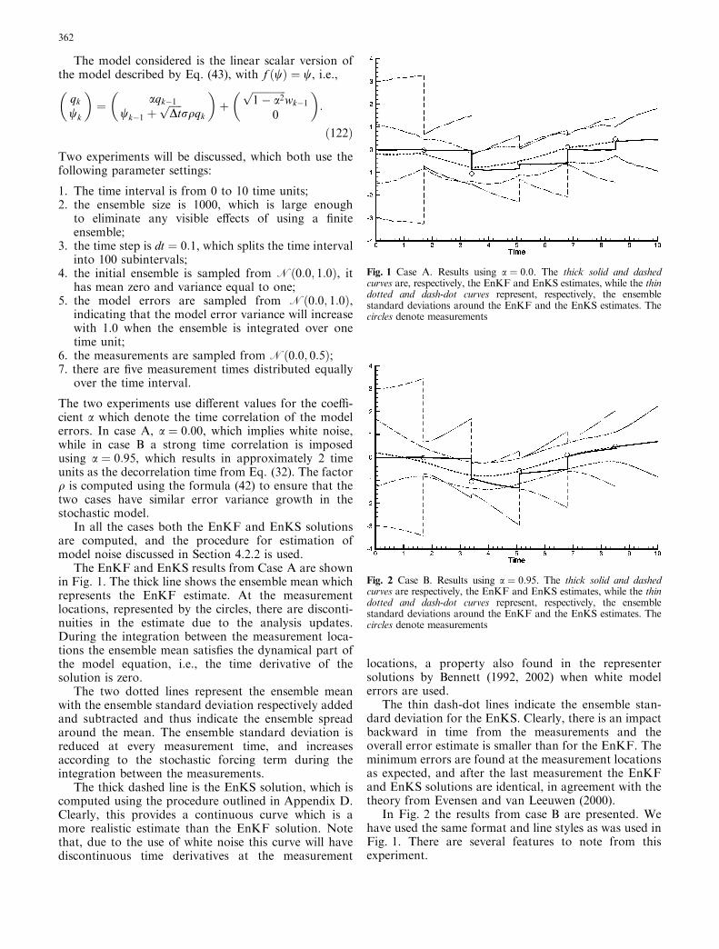
The model considered is the linear scalar version ofthe model described by Eq. (43), with f #w% " w, i.e.,

qk

wk

& '" aqk$1

wk$1 &!!!!!Dtp

rqqk

& '&

!!!!!!!!!!!!!1$ a2p

wk$10

& ':

#122%

Two experiments will be discussed, which both use thefollowing parameter settings:

1. The time interval is from 0 to 10 time units;2. the ensemble size is 1000, which is large enough

to eliminate any visible e!ects of using a finiteensemble;

3. the time step is dt " 0:1, which splits the time intervalinto 100 subintervals;

4. the initial ensemble is sampled from N#0:0; 1:0%, ithas mean zero and variance equal to one;

5. the model errors are sampled from N#0:0; 1:0%,indicating that the model error variance will increasewith 1.0 when the ensemble is integrated over onetime unit;

6. the measurements are sampled from N#0:0; 0:5%;7. there are five measurement times distributed equally

over the time interval.

The two experiments use di!erent values for the coe"-cient a which denote the time correlation of the modelerrors. In case A, a " 0:00, which implies white noise,while in case B a strong time correlation is imposedusing a " 0:95, which results in approximately 2 timeunits as the decorrelation time from Eq. (32). The factorq is computed using the formula (42) to ensure that thetwo cases have similar error variance growth in thestochastic model.

In all the cases both the EnKF and EnKS solutionsare computed, and the procedure for estimation ofmodel noise discussed in Section 4.2.2 is used.

The EnKF and EnKS results from Case A are shownin Fig. 1. The thick line shows the ensemble mean whichrepresents the EnKF estimate. At the measurementlocations, represented by the circles, there are disconti-nuities in the estimate due to the analysis updates.During the integration between the measurement loca-tions the ensemble mean satisfies the dynamical part ofthe model equation, i.e., the time derivative of thesolution is zero.

The two dotted lines represent the ensemble meanwith the ensemble standard deviation respectively addedand subtracted and thus indicate the ensemble spreadaround the mean. The ensemble standard deviation isreduced at every measurement time, and increasesaccording to the stochastic forcing term during theintegration between the measurements.

The thick dashed line is the EnKS solution, which iscomputed using the procedure outlined in Appendix D.Clearly, this provides a continuous curve which is amore realistic estimate than the EnKF solution. Notethat, due to the use of white noise this curve will havediscontinuous time derivatives at the measurement

locations, a property also found in the representersolutions by Bennett (1992, 2002) when white modelerrors are used.

The thin dash-dot lines indicate the ensemble stan-dard deviation for the EnKS. Clearly, there is an impactbackward in time from the measurements and theoverall error estimate is smaller than for the EnKF. Theminimum errors are found at the measurement locationsas expected, and after the last measurement the EnKFand EnKS solutions are identical, in agreement with thetheory from Evensen and van Leeuwen (2000).

In Fig. 2 the results from case B are presented. Wehave used the same format and line styles as was used inFig. 1. There are several features to note from thisexperiment.

Fig. 1 Case A. Results using a " 0:0. The thick solid and dashedcurves are, respectively, the EnKF and EnKS estimates, while the thindotted and dash-dot curves represent, respectively, the ensemblestandard deviations around the EnKF and the EnKS estimates. Thecircles denote measurements

Fig. 2 Case B. Results using a " 0:95. The thick solid and dashedcurves are respectively, the EnKF and EnKS estimates, while the thindotted and dash-dot curves represent, respectively, the ensemblestandard deviations around the EnKF and the EnKS estimates. Thecircles denote measurements

362

The EnKF solution now sometimes shows a positiveor negative trend during the integration between themeasurements. This is caused by the assimilation up-dates of the model noise which introduces a ‘‘bias’’ in thestochastic forcing. An explanation for this can be foundby examining Fig. 3 which plots the EnKF solution asthe dashed line, the EnKF estimate for the model noiseas the thick solid line, and the standard deviation of themodel noise is plotted as the dotted lines. It is clearlyseen that the model noise is being updated at theassimilation steps, e.g., the second measurement indi-cates that the solution is around $1. This leads to anupdate of the model ensemble toward the measurement,as well as an introduction of a negative bias in the sys-tem noise. This is the negative bias which previouslyshould have been used in the model to achieve a betterprediction of this particular measurement. In the con-tinued integration this bias starts working until it iscorrected to become a positive bias at the next assimi-lation step. Note that during the integration between themeasurements the bias slowly relaxes back toward zeroas was discussed in Section 4.2.2.

The EnKS solution in case B is smoother than incase A and there are no longer discontinuous timederivatives at the measurement locations. Further, thestandard deviation for the EnKS is smoother and indi-cates that the impact of the measurements is carriedfurther backward in time.

The estimated EnKS system noise is presented as thethick solid line in Fig. 4 and also here the time deriva-tives are continuous at the measurement locations. Infact, this estimated model noise is the forcing needed toreproduce the EnKS solution when a single model isintegrated forward in time starting from the initial con-dition estimated by the EnKS. That is, the solution of

wk " wk$1 &!!!!!Dtp

rqqqk

w0 " ww0

#123%

with qqk and ww0 being the EnKS estimated model noiseand initial condition, respectively, will exactly reproducethe EnKS estimate.

This is illustrated by the two similar curves in Fig. 4,i.e., the dashed curve which is the EnKS estimate, andthe dash-dot-dot curve which is the solution of themodel forced by the estimated EnKS model noise (notethat the curves are nearly identical and a number 0.1 wassubtracted to make it easier to distinguish the curves).Obviously, the estimated model noise is the same as iscomputed and used in the forward Euler Lagrangeequation in the representer method (Bennett, 1992,2002). This points to the similarity between the EnKSand the representer method, which for linear models willgive identical results when the ensemble size becomesinfinite.

Appendix G: Bias and parameter estimation

The estimation of poorly known model parameters orbiases in dynamical models has been discussed by, e.g.,Evensen at al. (1998) and the references cited therein.The following examples will illustrate how the EnKFand EnKS may be used for parameter and bias estima-tion.

Note first, that the distinction between model biasand time correlated model errors is not clear. As anexample, one can envisage an ocean model which over-estimates a variable during summer and underestimatesit during winter. This could happen if a constant is usedto represent a process which changes slowly on theseasonal time scale. In a multiyear simulation, the poorrepresentation of this process should be interpreted as atime-correlated model error. However, if the model isused only for short simulations, one could also consider

Fig. 3 Case B. The thick solid line is the EnKF estimate of the modelnoise. The dotted lines show the standard deviation of the model noiseensemble around the EnKF estimate of the model noise. The dashedline is the EnKF estimate as shown in Fig. 2

Fig. 4 Case B. The thick solid line is the EnKS estimate of the modelnoise. The dotted lines show the standard deviation of the model noiseensemble around the EnKS estimate of the model noise. The dashedline is the EnKS estimate as shown in Fig. 2. The dash-dot-dot line isthe EnKS estimate computed from the forward model (123) but witha number 0.1 subtracted from the result to make it possible todistinguish the two curves

363

this error to be a model bias since it appears to beconstant on short time scales.

The following model system based on Eq. (122) willnow be examined in two examples to illustrate the im-pact of a model bias,

qk

bk

wk

0

B@

1

CA "aqk$1

bk$1

wk$1 & #g& bk%Dt &!!!!!Dtp

rqqk

0

B@

1

CA

&

!!!!!!!!!!!!!1$ a2p

wk$1

0

0

0

B@

1

CA: #124%

In the dynamical model we have now included a ‘‘trendterm’’, g, which states that the model solution as pre-dicted by the deterministic model should have the slope g.In the examples below g " 1:0, while the measurementsare simulated under the assumption that g " 0:0. Wehave also included an unknown bias parameter bk, whichwill be estimated to correct for the model bias introducedby the trend term. An additional equation is introducedfor the bias bk, stating that it should be stationary in time.

Two examples will be discussed next. In both of themwe set the following parameters in addition to the onesused in cases A and B:

1. The trend term g " 1:0, i.e., the model always pre-dicts a slope equal to one;

2. the initial condition is w0 2N#2:0; 1:0% (2.0 is choseninstead of 0.0 to make it easier to interpret the plots);

3. the measurements are sampled from N#2:0; 0:5%;4. the model error has a time correlation given by

a " 0:99, indicating strong correlation in time withapproximately 10 days decorrelation time;

5. the time interval is from 0 to 50 time units, with thesame Dt as before;

6. the total number of measurements is 25 which givesthe same measurement density in time as before.

In case C we will not attempt to estimate any bias termand the initial statistics for b is N#0:0; 0:0%, i.e., zeromean and variance. The purpose is to examine how atime-correlated model error can correct for the modelbias. The results from case C are shown in Fig. 5 for theEnKF (upper plot), and EnKS (lower plot) respectively.In the EnKF case it is seen how the model trend termwith g " 1:0 introduces a positive drift during theensemble integration, resulting in an overestimate atmeasurement times. The estimated model error has anegative trend and varies around $1, thus it partlycompensates for the positive model bias. However, thenature of the stocastic forcing is to relax back towardszero between the measurement updates and it will notconverge towards a fixed value. For the EnKS the situ-ation is similar. The estimate smooths the measurementsvery well, and the estimated model error is varyingaround $1 to compensate for the positive trend term inthe model. Thus, the use of time-correlated model errorsmay compensate for possible model biases.

In case D we set the statistics for b to be N#0:0; 2:0%,i.e., our first guess of the model bias is zero, but weassume that the error in this guess has variance equal to2.0. The results from case D are given in Fig. 6 for theEnKF (upper plot) and EnKS (lower plot) respectively.

In the EnKF case, the estimated model bias termconverges toward a value bk " $0:845. Thus, it accountsfor, and corrects, 84.5% of the model bias introduced bythe trend term g. The estimate will always be locatedsomewhere between the first guess, b0 " 0:0, and the biaswhich is$1:0. A better fit to$1 can be obtained by usinga larger variance on the first guess of b or by assimilatingadditional measurements. The model error term nowvaries around 0:0 possibly with a small negative trendwhich accounts for the uncorrected 15:5% of the bias.

In the EnKS case, the estimated bias is a constantthrough-out the time interval. This is obvious since thereis no dynamical evolution of bk, thus bk is constructedfrom:

bk " b0

Y25

i"1X5#i%; 8k: #125%

Fig. 5 Case C. The upper plot shows the EnKF estimate as the thicksolid line and the estimated model error as the dashed line. The lowerplot shows the EnKS estimate as the thick solid line while the dottedlines indicate the standard deviation of the estimate. The estimatedmodel error is plotted as the dashed line

364

The value for b is also equal to the final value obtainedby the EnKF. Thus, there is no improvement obtainedin the estimate for b by using the EnKS (see Fig. 7).Figure 7 also illustrates the convergence over time of thebias estimates and their error bars. Also in the EnKS themodel error is varying around zero but with a weak

negative trend. Thus, it is possible to use the EnKF andEnKS for parameter and bias estimation in dynamicalmodels.

Acknowledgements I would like to express my thanks and gratitudeto co-workers at the Nansen Center and elsewhere for providingvaluable inputs and stimulating discussions during the work withthis paper. In particular I would like to thank L. Bertino, K. A.Lister, Y. Morel, L. J. Natvik, D. Obaton, and H. Sagen, who havehelped implementing and testing the new algorithms, checkedderivations and contributed to making this paper readable andhopefully useful for the community developing ensemble methodsfor data assimilation. I am also grateful for comments by twoanonymous reviewers, which helped me to improve the consistencyof the paper. This work was supported by the EC FP–5 projectsTOPAZ (EVK3-CT2000-00032) and ENACT (EVK2-CT-2001-00117), and has received support from The Research Council ofNorway (Programme for Supercomputing) through a grant ofcomputing time.

References

Allen JI, Eknes M, Evensen G (2002) An Ensemble Kalman Filterwith a complex marine ecosystem model: hindcasting phyto-plankton in the Cretan Sea. Annal Geophys 20: 1–13

Anderson JL (2001) An ensemble adjustment Kalman filter fordata assimilation. Mon Weather Rev 129: 2884–2903

Anderson JL (2003) A local least-squares framework for ensemblefiltering. Mon Weather Rev 131: 634–642

Anderson JL, Anderson SL (1999) A Monte Carlo implementationof the nonlinear filtering problem to produce ensemble assimi-lations and forecasts. Mon Weather Rev 127: 2741–2758

Bennett AF (1992) Inverse methods in physical oceanography.Cambridge University Press, Cambridge

Bennett AF (2002) Inverse modeling of the ocean and atmosphere.Cambridge University Press, Cambridge

Bennett AF, Chua BS (1994) Open-ocean modeling as an inverseproblem: the primitive equations. Mon Weather Rev 122: 1326–1336

Bennett AF, Leslie LM, Hagelberg CR, Powers PE (1993) Tropicalcyclone prediction using a barotropic model initialized by ageneralized inverse method. Mon Weather Rev 121: 1714–1729

Bennett AF, Chua BS, Leslie LM (1996) Generalized inversion of aglobal numerical weather prediction model. Meteorol AtmosPhys 60: 165–178

Bertino L, Evensen G, Wackernagel H (2002) Combining geosta-tistics and Kalman filtering for data assimilation in an estuarinesystem. Inverse Methods 18: 1–23

Bishop CH, Etherton BJ, Majumdar SJ (2001) Adaptive samplingwith the ensemble transform Kalman filter. part I. Theoreticalaspects. Mon Weather Rev 129: 420–436

Bleck R, Rooth C, Hu D, Smith LT (1992) Salinity-driven ther-mohaline transients in a wind- and thermohaline-forcedisopycnic coordinate model of the North Atlantic. J PhysOceanogr 22: 1486–1515

Brasseur P, Ballabrera J, Verron J (1999) Assimilation of alti-metric data in the mid-latitude oceans using the SEEK filterwith an eddy-resolving primitive equation model. J Marine Sys22: 269–294

Brusdal K, Brankart J, Halberstadt G, Evensen G, Brasseur P, vanLeeuwen PJ, Dombrowsky E, Verron J (2003) An evaluation ofensemble based assimilation methods with a layered OGCM.J Marine Sys 40-41: 253–289

Burgers G, van Leeuwen PJ, Evensen G (1998) Analysis scheme inthe ensemble Kalman Filter. Mon Weather Rev 126: 1719–1724

Carmillet V, Brankart JM, Brasseur P, Drange H, Evensen G(2001) A singular evolutive extended Kalman filter to assimilateocean color data in a coupled physical-biochemical model of theNorth Atlantic. Ocean Modelling 3: 167–192

Fig. 6 Case D. Same as Fig. 5 but with the additional dash-dot lineshowing the estimated bias for the EnKF and the EnKS

Fig. 7 Case D. The time evolution of the bias estimates from theEnKF (solid line) and the EnKS (dashed line), with the error standarddeviations for the EnKF (dotted line) and the EnKS (dash-dot line)

365

Courtier P (1997) Dual formulation of variational assimilation.Q J R Meteorol Soc 123: 2449–2461

Courtier P, Talagrand O (1987) Variational assimilation of mete-orological observations with the adjoint vorticity equation II:numerical results. Q J R Meteorol Soc 113: 1329–1347

Courtier P, Thepaut, Hollingsworth A (1994) A strategy foroperational implementation of 4DVAR, using an incrementalapproach. Q J R Meteorol Soc 120: 1367–1387

Crow WT, Wood EF (2003) The assimilation of remotely sensedsoil brightness temperature imagery into a land surface modelusing Ensemble Kalman Filtering: a case study based on ES-TAR measurements during SGP97. Adv Water Resources 26:137–149

Echevin V, Mey PD, Evensen G (2000) Horizontal and verticalstructure of the representer functions for sea surface measure-ments in a coastal circulation model. J Phys Oceanogr 30: 2627–2635

Eknes M, Evensen G (2002) An Ensemble Kalman Filter with a1-D marine ecosystem model. J Marine Sys 36: 75–100

Evensen G (1992) Using the extended Kalman filter with a multi-layer quasi-geostrophic ocean model. J Geophys Res 97(C11):17 905–17 924

Evensen G (1994a) Inverse Methods and data assimilation innonlinear ocean models. Physica (D) 77: 108–129

Evensen G (1994b) Sequential data assimilation with a non-linearquasi-geostrophic model using Monte Carlo methods to fore-cast error statistics. J Geophys Res 99(C5): 10 143–10 162

Evensen G (1997) Advanced data assimilation for strongly non-linear dynamics. Mon Weather Rev 125: 1342–1354

Evensen G, van Leeuwen PJ (1996) Assimilation of Geosat alti-meter data for the Agulhas Current using the Ensemble KalmanFilter with a quasi-geostrophic model. Mon Weather Rev 124:85–96

Evensen G, van Leeuwen PJ (2000) An Ensemble KalmanSmoother for nonlinear dynamics. Mon Weather Rev 128:1852–1867

Evensen G, Dee D, Schroter J (1998) Parameter estimation indynamical models. In: Chassignet EP, Verron J (eds.) Oceanmodeling and parameterizations Kluwer Academic, TheNederlands, pp 373–398

Ggradshteyn IS, Ryzhik IM (1979) Table of integrals, series, andproducts: corrected and enlarged edition. Academic Press, Newyork

Grønnevik R, Evensen G (2001) Application of ensemble basedtechniques in fish-stock assessment. Sarsia 86: 517– 526

Hamill TM, Snyder C (2000) A hybrid Ensemble Kalman Filter–3 D variational analysis scheme. Mon Weather Rev 128: 2905–2919

Hamill TM, Mullen SL, Snyder C, Toth Z, Baumhefner DP (2000)Ensemble forecasting in the short to medium range: report froma workshop. Bull Am Meteorol Soc 81(11): 2653–2664

Hamill TM, Whitaker JS, Snyder C (2001) Distance-dependentfiltering of background error covariance estimates in anEnsemble Kalman Filter. Mon Weather Rev 129: 2776–2790

Hansen JA, Smith LA (2001) Probabilistic noise reduction. Tellus,Ser (A) 53: 585–598

Haugen VE, Evensen G (2002) Assimilation of SLA and SST datainto an OGCM for the Indian ocean. Ocean Dynamics 52: 133–151

Haugen VE, Evensen G, Johannessen OM (2002) Indian Oceancirculation: an integrated model and remote sensing study.J Geophys Res 107(C5): 11–1–11–23

Heemink AW, Verlaan M, Segers AJ (2001) Variance reducedensemble Kalman Filtering. Mon Weather Rev 129: 1718– 1728

Houtekamer PL, Mitchell HL (1998) Data assimilation using anEnsemble Kalman Filter technique. Mon Weather Rev 126:796–811

Houtekamer PL, Mitchell HL (1999) Reply. Mon Weather Rev127: 1378–1379

Houtekamer PL, Mitchell HL (2001) A sequential ensembleKalman filter for atmospheric data assimilation. Mon WeatherRev 129: 123–137

Jazwinski AH (1970) Stochastic processes and filtering theory.Academic, San Diego, California

Keppenne CL (2000) Data assimilation into a primitive-equationmodel with a parallel Ensemble Kalman Filter. Mon WeatherRev 128: 1971–1981

Keppenne CL, Rienecker M (2003) Assimilation of Temperatureinto an isopycnal ocean general circulation model using aparallel Ensemble Kalman Filter. J Mar Sys 40-41: 363–380

Lermusiaux PFJ (2001) Evolving the subspace of the three-dimensional ocean variability: Massachusetts Bay. J Marine Sys29: 385–422

Lermusiaux PFJ, Robinson AR (1999a) Data assimilation via errorsubspace statistical estimation. part I. Theory and schemes.Mon Weather Rev 127: 1385–1407

Lermusiaux PFJ, Robinson AR (1999b) Data assimilation via errorsubspace statistical estimation, part II. Middle Atlantic Bightshelfbreak front simulations and ESSE validation. MonWeather Rev 127: 1408–1432

Madsen H, Canizares R (1999) Comparison of Extended andEnsemble Kalman filters for data assimilation in coastal areamodelling. Int J Numer Meth Fluids 31: 961–981

Majumdar SJ, Bishop CH, Etherton BJ, Szunyogh I, Toth Z (2001)Can an ensemble transform Kalman filter predict the reductionin forecast-error variance produced by targeted observations?Q J R Meteorol Soc 127: 2803–2820

Miller RN, Ehret LL (2002) Ensemble generation for models ofmultimodal systems. Mon Weather Rev 130: 2313–2333

Miller RN, Ghil M, Gauthiez F (1994) Advanced data assimilationin strongly nonlinear dynamical systems. J Atmos Sci 51: 1037–1056

Miller RN, Carter EF, Blue ST (1999) Data assimilation intononlinear stochastic models. Tellus Ser (A) 51: 167–194

Mitchell HL, Houtekamer PL (2000) An adaptive Ensemble Kal-man Filter. Mon Weather Rev 128: 416–433

Mitchell HL, Houtekamer PL, Pellerin G (2002) Ensemble size,and model-error representation in an Ensemble Kalman Filter.Mon Weather Rev 130: 2791–2808

Natvik LJ (2001) A data assimilation system for a 3– dimensionalbiochemical model of the North Atlantic. PhD Thesis, Uni-versity of Bergen/Nansen Environmental and Remote SensingCenter, Edv. Griegsv 3a, 5059 Bergen, Norway

Natvik LJ, Evensen G (2003a) Assimilation of ocean colour datainto a biochemical model of the North Atlantic, part 1. Dataassimilation experiments. J Marine Sys 40-41: 127–153

Natvik LJ, Evensen G (2003b) Assimilation of ocean colour datainto a biochemical model of the North Atlantic, part 2. Sta-tistical analysis. J Marine Sys 40-41: 155–169

Park JH, Kaneko A (2000) Assimilation of coastal acoustictomography data into a barotropic ocean model. Geophys ResLett 27: 3373–3376

Pham DT (2001) Stochastic methods for sequential data assimila-tion in strongly nonlinear systems. Mon Weather Rev 129:1194–1207

Pham DT, Verron J, Roubaud MC (1998) A singular evolutiveextended Kalman Filter for data assimilation in oceanography.J Marine Sys 16: 323–340

Reichle RH, McLaughlin DB, Entekhabi D (2002) Hydrologic dataassimilation with the Ensemble Kalman Filter. Mon WeatherRev 130: 103–114

Talagrand O, Courtier P (1987) Variational assimilation of mete-orological observations with the adjoint vorticity equation. I:Theory. Q J R Meteorol Soc 113: 1311–1328

Thacker WC, Esenkov OE (2002) Assimilating XBT data intoHYCOM. J Atmos Ocean Tech 19: 709–724

Tippett MK, Anderson JL, Bishop CH, Hamill TM, Whitaker JS(2003) Ensemble square-root filters. Mon Weather Rev 131:1485–1490

Troccoli A, Balmaseda MA, Segschneider J, Vialard J, AndersonDLT (2002) Salinity adjustment in the presence of temperaturedata assimilation. Mon Weather Rev 130: 89–102

van Leeuwen PJ (1999a) Comment on ‘‘Data assimilation using anEnsemble Kalman Filter technique’’. Mon Weather Rev 127: 6

366

van Leeuwen PJ (1999b) The time mean circulation in the Agulhasregion determined with the Ensemble Smoother. J Geophys Res104: 1393–1404

van Leeuwen PJ (2001) An Ensemble Smoother with error esti-mates. Mon Weather Rev 129: 709–728

van Leeuwen PJ (2003) A variance-minimizing filter for large-scaleapplications. Mon Weather Rev (In press)

van Leeuwen PJ, Evensen G (1996) Data assimilation and inversemethods in terms of a probabilistic formulation. Mon WeatherRev 124: 2898–2913

van Loon M, Builtjes PJH, Segers AJ (2000) data assimilation ofozone in the atmoshperic transport chemistry model LOTUS.Environ Modelling Software 15: 603–609

Verlaan M, Heemink AW (2001) Nonlinearity in data assimilationapplications: a practical method for analysis. MonWeather Rev129: 1578–1589

Whitaker JS, Hamill TM (2002) Ensemble data assimilationwithout perturbed observations. Mon Weather Rev 130: 1913–1924

367