Embed Size (px)
Citation preview

Gaussian Factor Models - Futures and Forward Prices
Cody. B. HyndmanDepartment of Mathematics and Statistics, Concordia University
1455 boulevard de Maisonneuve Ouest
Montreal, Quebec
Canada H3G 1M8
email: [email protected]
March 10, 2007
Abstract
We completely characterise the futures price and forward price of a risky asset (commodity) paying
a stochastic dividend yield (convenience yield). The asset (commodity) price is modelled as an expo-
nential affine function of a Gaussian factors process while the interest rate and dividend yield are affine
functions of the factors process. The characterisation we provide is based on the method of stochastic
flows. We believe this method leads to simpler and more clear-cut derivations of the futures price and
forward price formulae than alternative methods. Hedging a long term forward contract with shorter
term futures contracts and bonds is also examined.
Keywords: futures price; forward price; stochastic flows; factor models; Gaussian state variables
The author would like to thank Andrew Heunis and Robert Elliott for helpful discussions.
The author would like to acknowledge the financial support of MITACS through the “Prediction in Interacting Sys-
tems (PINTS)” and “Modelling Trading and Risk in the Market” projects and the financial support of the Institut de finance
mathematique de Montreal (IFM2).

Gaussian Factor Models - Futures and Forward Prices 2
1 Introduction
Gaussian factor models of asset prices have been extensively used in financial modelling. Gaussian models
remain popular due to their analytic tractability and well established statistical methodology. Continuous-
time models for futures and forward prices have been studied by Gibson and Schwartz (1990), Schwartz
(1997, 1998), Cortazar and Schwartz (1994), Miltersen and Schwartz (1998), Schwartz and Smith (2000),
and Manoliu and Tompaidis (2002) among others. The work of Miltersen and Schwartz (1998) is notable
in that it develops an analogue of the Heath, Jarrow and Morton (1992) model in the context of futures
markets. Other general studies on futures and forward prices include Schroder (1999), Bjork and Landen
(2002), and the references contained therein.
In this paper we completely characterise the futures price and forward price of a risky asset (commodity)
paying a stochastic dividend yield (convenience yield). The interest rate and dividend yield are modelled
as affine functions of a Gaussian factors process. We also assume that the asset price is modelled as
an exponential affine function of the Gaussian factors process. Our analysis is based on the method
of stochastic flows introduced to the term structure literature by Elliott and van der Hoek (2001). The
stochastic flows method presented in this paper includes the Gaussian factors models which have appeared
in the literature as a special case and has been generalized to include models which include non-Gaussian
(square-root or Cox, Ingersoll and Ross (1985) type) factors. One of the main contributions of this paper
is a unified framework under which to study a wide class of models in a systematic and clear-cut way.
Most of the derivations of futures and forward prices which have appeared in the literature, with the excep-
tion of Bjork and Landen (2002), have been model specific and do not address the entire class of Gaussian
factor models. Derivations of futures and forward prices that have appeared in the literature have usually
been based on solving a partial differential equation (PDE) or calculating a conditional expectation using
the distributional properties of the factors process. However, in the case of PDE derivations the exponen-
tial affine form of the solution is guessed and then substituted into the PDE to reduce the problem to the
solution of ordinary differential equations (ODEs). Our method shows why the solution is exponential
affine by characterizing the futures and forward price as the solution to a linear ODE. Derivations of the
prices based on distributional properties of the factors process, for example Bjerksund (1991), are often
complicated when some factors are correlated. Further, our method has been generalised to study other
models, outside the assumptions of this paper, where the functional form of the solution to the PDE for
the contingent claim is not easily guessed.

Gaussian Factor Models - Futures and Forward Prices 3
Due to certain shortcomings of Gaussian models, or the desire to better model asset price movements,
more complicated models which often incorporate non-Gaussian components and jumps have become
widely used. For example Yan (2002), Bjork and Landen (2002), and Ribeiro and Hodges (2004) em-
ploy combinations of Gaussian, non-Gaussian, and jump factors. For non-Gaussian factor models certain
approximations and assumptions, often left unjustified, are made to allow for a practical implementation
of the model or to calibrate the model to historical data. For models containing a combination of Gaus-
sian and Cox, Ingersoll and Ross (1985) type factors the validity of applying the Feynman-Kac formula
to derive derivative prices has only been recently justified by Levendorskiı (2004) despite the previous
appearance of such models and derivations in the literature.
The methods of this paper have been extended to ‘affine term structure models’ and ‘affine price mod-
els’ in Hyndman (2005) where the factors process follows an affine diffusion. This extension includes
as special cases the continuous factors model of Duffie and Kan (1996) for bond prices and Bjork and
Landen (2002) for futures and forward prices. Additional tools, namely changes of measure and forward-
backward stochastic differential equations, are required to derive the bond, futures, and forward prices for
general affine factor models which are not required in the Gaussian case. Therefore, we shall concentrate
exclusively on the Gaussian case in this paper.
The remainder of this paper is organised as follows. Section 2 discusses the market model and sets some
notation. Section 3 studies the futures price, Section 4 reviews some results on the bond price which are
necessary for our discussion of the forward price in Section 5, and Section 6 examines hedging a long
term forward commitment using shorter term futures contracts and bonds. Section 7 briefly discusses
implementation and the estimation of model parameters, Section 8 shows how our methods apply to three
different commodity market models that have appeared in the literature, and Section 9 concludes.
2 Market Model
Let (Ω,F ,P) be a complete probability space on which there is given a standard, m-dimensional Brownian
motion Wt = (W (1)t , . . . ,W (m)
t )′ with ′ denoting the transpose. For a fixed, positive, and finite time horizon
T ∗ define F Wt = σ(Wu : 0 ≤ u ≤ t) for all t ∈ [0,T ∗]. Let N denote the P-null subsets of F W
T ∗ . The filtration
generated by W and augmented by the null sets, Ft = σ(F Wt ∪N ), models the information available to
investors and should be regarded as fixed. That is, we cannot choose to work with a different filtration.
The modelling framework is the filtered probability space (Ω,F ,Ft , t ≥ 0,P). To avoid repeating the

Gaussian Factor Models - Futures and Forward Prices 4
entire development of classical mathematical finance we take the following as given.
Assumption 2.1 Throughout we shall assume a complete and standard financial market in the sense of
Definitions 1.5.1 and 1.6.1 of Karatzas and Shreve (1998).
Under Assumption 2.1 there exists a unique equivalent martingale measure Q on FT ∗ . The practical
advantage of working with the measure Q is that the prices of derivative securities can be expressed as
conditional expectations.
On (Ω,F ,Q) consider a factors process X taking values in Rn given by
dXt = (AtXt + γt)dt +σtdBt (1)
where B is any m-dimensional Brownian motion with respect to the fixed filtration Ft , t ≥ 0 and the
risk-neutral measure Q. In particular the usual Brownian motion constructed using Girsanov’s Theorem
as in Karatzas and Shreve (1998, p. 17) can be used. Also, At is a time-varying (deterministic) (n× n)-
matrix, γt is a time-varying (deterministic) (n×1)-column vector, and σt is a time-varying (deterministic)
(n×m)-matrix. Further, we require the functions γ : [0,T ]→ Rn, A : [0,T ]→ Rn×n, and σ : [0,T ]→ Rn×m
to be Borel measurable, integrable, and globally Lipschitz so that the SDE (1) has a unique strong solution.
Assumption 2.2 We assume that the riskless interest rate, the asset (spot) price, and the dividend (conve-
nience) yield are functions of the factors process. That is,
rt = r(Xt), St = S(Xt), and δt = δ(Xt).
where r : Rn → R, δ : Rn → R, and S : Rn → R++ are specified by:
(i) rt = r(Xt) where, for x ∈ Rn, r(x) = R′x+ k, R is an (n×1)-column vector, and k is a scalar;
(ii) St = S(Xt) where, for x ∈ Rn, S(x) = exp(M′x+h), M is an (n× 1)-column vector, and h is a
scalar; and
(iii) δt = δ(Xt) where, for x ∈ Rn, δ(x) = N′x+ l, N is an (n×1)-column vector, and l is a scalar.
The process rt given by this setup can take negative values with positive probability. However, the Vasıcek
(1977) and Hull and White (1994) interest rate models are special cases of the general Gaussian factors
Gaussian Factor Models - Futures and Forward Prices 5
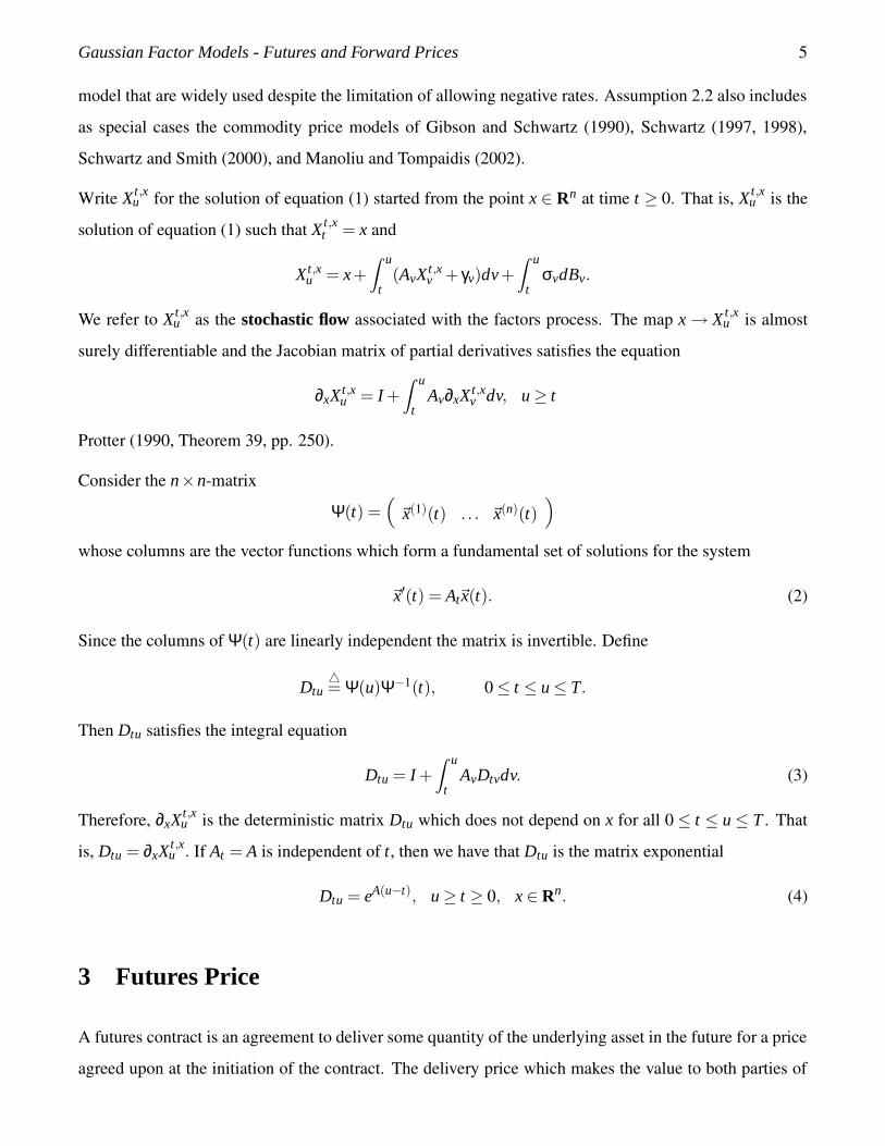
model that are widely used despite the limitation of allowing negative rates. Assumption 2.2 also includes
as special cases the commodity price models of Gibson and Schwartz (1990), Schwartz (1997, 1998),
Schwartz and Smith (2000), and Manoliu and Tompaidis (2002).
Write X t,xu for the solution of equation (1) started from the point x ∈ Rn at time t ≥ 0. That is, X t,x
u is the
solution of equation (1) such that X t,xt = x and
X t,xu = x+
Z u
t(AvX t,x
v + γv)dv+Z u
tσvdBv.
We refer to X t,xu as the stochastic flow associated with the factors process. The map x → X t,x
u is almost
surely differentiable and the Jacobian matrix of partial derivatives satisfies the equation
∂xX t,xu = I +
Z u
tAv∂xX t,x
v dv, u ≥ t
Protter (1990, Theorem 39, pp. 250).
Consider the n×n-matrix
Ψ(t) =(
~x(1)(t) . . . ~x(n)(t))
whose columns are the vector functions which form a fundamental set of solutions for the system
~x′(t) = At~x(t). (2)
Since the columns of Ψ(t) are linearly independent the matrix is invertible. Define
Dtu4= Ψ(u)Ψ−1(t), 0 ≤ t ≤ u ≤ T.
Then Dtu satisfies the integral equation
Dtu = I +Z u
tAvDtvdv. (3)
Therefore, ∂xX t,xu is the deterministic matrix Dtu which does not depend on x for all 0 ≤ t ≤ u ≤ T . That
is, Dtu = ∂xX t,xu . If At = A is independent of t, then we have that Dtu is the matrix exponential
Dtu = eA(u−t), u ≥ t ≥ 0, x ∈ Rn. (4)
3 Futures Price
A futures contract is an agreement to deliver some quantity of the underlying asset in the future for a price
agreed upon at the initiation of the contract. The delivery price which makes the value to both parties of

Gaussian Factor Models - Futures and Forward Prices 6
the contract zero at all times is called the futures price. By the mechanism of marking to market, where
changes in the value of the futures contract are settled daily, in accordance with changes in the futures
price the risk of default by one party is transfered to the exchange. Basic information on futures contracts
and market mechanics can be found in Hull (2002).
In this section we shall characterise the futures price as an exponential affine function of the factors pro-
cess, whose dynamics are given by (1), when the market model satisfies Assumptions 2.1 and 2.2. By
Assumption 2.1 the futures price of the risky asset S is given by
G(t,T ) = EQ[ST |Ft ] (5)
at time t for maturity T (see Karatzas and Shreve (1998, Theorem 3.7, pp. 45-46) for a proof). The
result upon which our methods and results are based is the following version of the Markov property (see
Friedman (1975) for a more general result and proof).
Proposition 3.1 For 0 ≤ t ≤ T
G(t,T ) = G(t,T,Xt)
Q−a.s, where for x ∈ Rn we define
G(t,T,x)4= EQ[S(X t,x
T )]. (6)
The notation G(t,T,x) introduced in Proposition 3.1 can be confused with the notation for the futures
price. However, G(t,T,x) is not a price per se, rather, it is a function expressing the dependence of the
futures price on the factors of the economy at time t. If we can completely understand the functional
dependence of G(t,T,x) on (t,T,x) then Proposition 3.1 allows us to understand the dependence of the
futures price on the factors and sensitivities to changes in the factors.
By differentiating G(t,T,x) with respect to x (denoted by ∂xG(t,T,x)) we obtain, subject to regularity
conditions that allow the exchange of expectation and differentiation, that
∂xG(t,T,x) = EQ[S(X t,xT )D
′tT M]. (7)
Since D′tT M is deterministic it can be brought outside of the expectation and we obtain the following result
which shall be used to characterise the futures price as an exponential affine function of the factors.
Theorem 3.2 For 0 ≤ t ≤ T
∂xG(t,T,x) = D′tT MG(t,T,x) (8)
for all x ∈ Rn.

Gaussian Factor Models - Futures and Forward Prices 7
The solution of the (system of) linear ODE (8) is an exponential affine function of x and, from equation
(6), the terminal condition is G(T,T,x) = S(x).
Corollary 3.3 For 0 ≤ t ≤ T
G(t,T,x) = exp(M′DtT x+L(t,T )). (9)
for all x ∈ Rn and some non-random function L(t,T ) such that L(T,T ) = h, where h is defined in Assump-
tion 2.2 (ii).
Applying Proposition 3.1 to equation (9) gives
Theorem 3.4 For 0 ≤ t ≤ T
G(t,T ) = exp(M′DtT Xt +L(t,T ))
Q−a.s.
We now turn our attention to representing L(t,T ) as the solution of an ODE. Note that for any vector b we
write bi for the i-th element and for any matrix Σ we write Σi j for the (i, j)-th element.
Theorem 3.5 G(t,T,x) satisfies the PDE
0 =∂G(t,T,x)
∂t+
∂G′(t,T,x)∂x
[Atx+ γt ]+12
n
∑i=1
n
∑j=1
∂2G(t,T,x)∂xi∂x j
[σtσ′t ]i j (10)
for all (t,x) ∈ [0,T ]×Rn with G(T,T,x) = S(x).
Proof: For all (t,x) ∈ [0,T ]×Rn define b(t,x) = [Atx + γt ], σ(t,x) = σt , and a(t,x) = σ(t,x)σ′(t,x) so
that
aik(t,x) = ∑mj=1 σi j(t,x)σk j(t,x) 1 ≤ i,k ≤ n.
Consider the operator At defined, for f ∈C2(Rn), by
(At f )(x) =12
n
∑i=1
n
∑k=1
aik(t,x)∂ f (x)∂xi∂x j
+n
∑i=1
bi(t,x)∂ f (x)
∂xi.
By the Feynman-Kac formula, Karatzas and Shreve (1991, pp. 366-367), there exists v(t,x) : [0,T ]×Rn →Rn such that v ∈C1,2([0,T ]×Rn), satisfies the Cauchy problem
−∂v∂t
= Atv ; in [0,T )×Rn,
v(T,x) = S(x) ; x ∈ Rn,

Gaussian Factor Models - Futures and Forward Prices 8
and
v(t,x) = EQ[S(X t,xT )]
is the unique solution. Therefore, by equation (6) we have
v(t,x) = G(t,T,x) ∀(t,x) ∈ [0,T ]×Rn.
Hence, G(t,T,x) satisfies the PDE (10).
Corollary 3.6 L(t,T ) satisfies the ODE
0 =∂∂t
L(t,T )+M′DtT γt +
12
n
∑i=1
n
∑j=1
[D′tT MM
′DtT ]i j(σtσ
′t)i j (11)
for all t ∈ [0,T ], with terminal condition L(T,T ) = h and h is defined in Assumption 2.2 (ii).
Proof: Equation (11) follows by first calculating the partial derivatives of G(t,T,x) using equation (9).
Substituting these partial derivatives into equation (10), dividing by the positive quantity G(t,T,x), and
setting x = 0 gives equation (11).
The terminal condition follows by setting t = T in equation (6) to find G(T,T,x) = S(x) for all x ∈ Rn.
Then, with t = T , comparing equation (9) with Assumption 2.2 (ii) we must have
M′DT T x+L(T,T ) = M
′x+h
for all x ∈ Rn where h is from Assumption 2.2 (ii). However, from equation (3), DT T = I, the n×n identity
matrix, for all x ∈ Rn. Therefore, we must have L(T,T ) = h.
We shall show, in Section 8, that the general methodology presented in this section can be easily applied
to various examples of commodity market models found in the literature. We delay the examples until
after our discussion of the forward price so that we may consider the futures and forward price of a given
model simultaneously. In the next section we briefly review some results on the zero-coupon bond price
that are necessary for our discussion of the forward price.
4 Bond Price
The results of this section are based on results presented for affine term structure models and appeared
in Elliott and van der Hoek (2001). For ease of reference and unity of notation we recall here the results
necessary for our analysis of the forward price of the risky asset.

Gaussian Factor Models - Futures and Forward Prices 9
By Assumption 2.1 the price of the zero-coupon bond is given by
P(t,T ) = EQ[exp(−Z T
trudu)|Ft ] (12)
at time t for maturity T . For 0 ≤ t ≤ T , since Xt is a Markov process (Friedman, 1975), it follows that
P(t,T ) = P(t,T,Xt) (13)
Q−a.s, where for x ∈ Rn we define
P(t,T,x)4= EQ[exp(−
Z T
tr(X t,x
u )du)]. (14)
Therefore, if we characterise the dependence of P(t,T,x) on (t,T,x), the Markov property allows us to
understand the dependence of the bond price on the factors. Differentiating P(t,T,x) with respect to
the initial condition (denoted by ∂xP(t,T,x)), subject to regularity conditions that allow the exchange of
expectation and differentiation, we find
∂xP(t,T,x) = EQ[exp(−Z T
tr(X t,x
u )du)
(
−Z T
tD
′tuRdu
)
]. (15)
We define
B(t,T )4=
Z T
tD
′tuRdu. (16)
Since B(t,T ) is deterministic it may be brought outside of the expectation to obtain the following result
which is used to characterise the bond price as an exponential affine function of the factors.
Theorem 4.1 For 0 ≤ t ≤ T
∂xP(t,T,x) = −B(t,T )P(t,T,x) (17)
for all x ∈ Rn.
The solution of the (system of) ODE (17) is an exponential affine function of x and, from equation (14),
the terminal condition is P(T,T,x) = 1.
Corollary 4.2 For 0 ≤ t ≤ T and for all x ∈ Rn
P(t,T,x) = exp(A(t,T )−B′(t,T )x) (18)
where B(t,T ) is from equation (16) with B(T,T ) = 0, and some non-random function A(t,T ) such that
A(T,T ) = 0.

Gaussian Factor Models - Futures and Forward Prices 10
Applying the Markov property, equation (13), to equation (18) gives:
Theorem 4.3 For 0 ≤ t ≤ T
P(t,T ) = exp(A(t,T )−B′(t,T )Xt) (19)
Q−a.s, for some function A to be determined.
Similar to Corollary 3.6 the function A(t,T ) may be represented as the solution of an ODE by applying
the Feynman-Kac formula. However, as this result is not necessary in the sequel we shall proceed directly
to our discussion of the forward price.
5 Forward Prices
A forward contract is much the same as a futures contract in that a quantity of the asset is agreed to be
delivered at some time in the future. However, unlike a futures contract, the value of a forward contract is
only zero to both parties at the initiation of the contract. The forward price is the delivery price that satisfies
this constraint. Forward contracts, unlike futures contracts, are not settled daily (marked to market) but
only at the delivery time. Basic information on futures and forward contracts and market mechanics can
be found in Hull (2002).
By Assumption 2.1 the forward price of the risky asset S is given by
F(t,T ) =EQ[exp(−R T
t rudu)ST |Ft ]
P(t,T )(20)
at time t for maturity T , where P(t,T ) is the zero-coupon bond price (Karatzas and Shreve, 1998, pp.
43-45). In the absence of a stochastic dividend (convenience yield) the numerator of equation (20) reduces
to the current spot price St by the fact that Q is a martingale measure. In the case of deterministic interest
rates the discount factor in the conditional expectation of equation (20) can be brought outside and cancels
the denominator. That is, in the case of deterministic interest rates the forward price (20) of the risky asset
is equal to the futures price (5) as noted by Cox et al. (1981). Therefore, in both cases the results of the
previous two sections may be used to prove that the forward price is an exponential affine function of the
factors. As such, we shall only consider models which include stochastic interest rates and a stochastic
dividend (convenience) yield given by Assumption 2.2.
The Markov property (Friedman, 1975) gives

Gaussian Factor Models - Futures and Forward Prices 11
Proposition 5.1 For 0 ≤ t ≤ T
F(t,T ) = F(t,T,Xt)
Q-almost surely, where for x ∈ Rn we define
F(t,T,x)4=
EQ[exp(−R Tt r(X t,x
u )du)S(X t,xT )]
P(t,T,x)(21)
and P(t,T,x) is defined as in equation (14).
By differentiating F(t,T,x) with respect to x (denoted by ∂xF(t,T,x)), we obtain, subject to regularity
conditions that allow the exchange of expectation and differentiation
∂xF(t,T,x) =EQ[exp(−R T
t r(X t,xu )du)S(X t,x
T )(
−B(t,T )+D′tT M
)
]−F(t,T,x)∂xP(t,T,x)
P(t,T,x). (22)
Therefore, from equations (21) and (22) we find
∂xF(t,T,x) =
(
−B(t,T )+D′tT M
)
F(t,T,x)P(t,T,x)−F(t,T,x)∂xP(t,T,x)
P(t,T,x). (23)
Applying the result of Theorem 4.1, namely ∂xP(t,T,x) = −B(t,T )P(t,T,x), to equation (23) gives the
following result.
Theorem 5.2 For 0 ≤ t ≤ T
∂xF(t,T,x) = D′tT MF(t,T,x) (24)
for all x ∈ Rn.
The solution of the (system of) ODE (24) is an exponential affine function of x and, from equation (21),
the terminal condition is F(T,T,x) = S(x).
Corollary 5.3 For 0 ≤ t ≤ T
F(t,T,x) = exp(M′DtT x+C(t,T )). (25)
for all x ∈ Rn for some non-random function C(t,T ) such that C(T,T ) = h with h from Assumption 2.2 (ii).
Applying Proposition 5.1 to equation (25) gives
Theorem 5.4 For 0 ≤ t ≤ T
F(t,T ) = exp(M′DtT Xt +C(t,T ))
Q-almost surely, for some function C(t,T ) to be determined where C(T,T ) = h and h is from Assump-
tion 2.2 (ii).
Gaussian Factor Models - Futures and Forward Prices 12
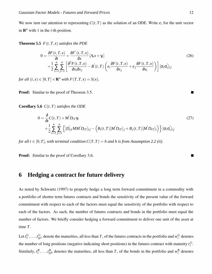
We now turn our attention to representing C(t,T ) as the solution of an ODE. Write ei for the unit vector
in Rn with 1 in the i-th position.
Theorem 5.5 F(t,T,x) satisfies the PDE
0 =∂F(t,T,x)
∂t+
∂F′(t,T,x)∂x
[Atx+ γt ] (26)
+12
n
∑i=1
n
∑j=1
[
∂2F(t,T,x)∂xi∂x j
−B′(t,T )
(
ei∂F(t,T,x)
∂x j+ e j
∂F(t,T,x)∂xi
)]
[σtσ′t ]i j
for all (t,x) ∈ [0,T ]×Rn with F(T,T,x) = S(x).
Proof: Similar to the proof of Theorem 3.5.
Corollary 5.6 C(t,T ) satisfies the ODE
0 =∂∂t
C(t,T )+M′DtT γt (27)
+12
n
∑i=1
n
∑j=1
[D′tT MM
′DtT ]i j −
(
Bi(t,T )[M′DtT ] j +B j(t,T )[M
′DtT ]i
)
[σtσ′t ]i j
for all t ∈ [0,T ], with terminal condition C(T,T ) = h and h is from Assumption 2.2 (ii).
Proof: Similar to the proof of Corollary 3.6.
6 Hedging a contract for future delivery
As noted by Schwartz (1997) to properly hedge a long term forward commitment in a commodity with
a portfolio of shorter term futures contracts and bonds the sensitivity of the present value of the forward
commitment with respect to each of the factors must equal the sensitivity of the portfolio with respect to
each of the factors. As such, the number of futures contracts and bonds in the portfolio must equal the
number of factors. We briefly consider hedging a forward commitment to deliver one unit of the asset at
time T .
Let tG1 , . . . , tG
NG denote the maturities, all less than T , of the futures contracts in the portfolio and wGi denotes
the number of long positions (negative indicating short positions) in the futures contract with maturity t Gi .
Similarly, tB1 , . . . , tB
NB denotes the maturities, all less than T , of the bonds in the portfolio and wBi denotes

Gaussian Factor Models - Futures and Forward Prices 13
the number of long positions in the bond with maturity tGi . Note n = NG + NB and to properly hedge the
forward commitment we must solve the following system of n equations in n unknowns.
NG
∑i=1
wGi e
′1D
′
ttGi
MG(t, tGi ,x)−
NB
∑i=1
wBi e
′1B(t, tB
i )P(t, tBi ,x) = e
′1
[
−B(t,T )+D′tT M
]
P(t,T,x)F(t,T,x)
...NG
∑i=1
wGi e
′nD
′
ttGi
MG(t, tGi ,x)−
NB
∑i=1
wBi e
′nB(t, tB
i )P(t, tBi ,x) = e
′n
[
−B(t,T )+D′tT M
]
P(t,T,x)F(t,T,x)
The choice of the number of futures contracts, NG, and the number of bonds, NB, to include in the portfolio
and at which maturities is not unique. However, such considerations are beyond the scope of this paper.
7 Statistical Estimation
One of the key features of Gaussian factor models and the resulting exponential affine form of the asso-
ciated bond, futures, and forward prices is the ease with which various statistical estimation techniques
can be used to calibrate the model parameters to market data. Further, if it is assumed that the factors
are unobservable while the term structure of bond, futures, or forward prices is observed over time the
Kalman filter can be employed to estimate the model parameters and the time series of the factors given
the observed term structure. Under a logarithmic transformation of the bond, futures, or forward price and
an Euler discretisation of the factors process a state-space model is obtained to which the discrete-time
Kalman filter can be applied. That is, if the term structure of futures prices G(tn,Ti) ; i = 1, . . . ,Mfor contracts expiring at times T1,T2, . . . ,TM is observed in the market at discrete times t0, t1, . . . , tNthen an empirical model to which we can apply the discrete-time (linear) Kalman filter is obtained by an
Euler discretisation of the real-world (P-measure) dynamics for the factors Xt and the ith component of the
observation vector is Y in = logG(tn,Ti)+“noise” with G(t,T ) given by Theorem 3.4.
This procedure has been employed, for example, by Babbs and Nowman (1999) in the case of interest
rates and by Schwartz (1997), Schwartz and Smith (2000), and Manoliu and Tompaidis (2002) in the case
of commodity markets and futures prices. In each case parameters were estimated by direct maximization
of the likelihood function and the factors were estimated by the Kalman filter from the observable term-
structure. An overview of the Kalman filter and maximum likelihood estimation, as well as an alternative
to direct maximization of the likelihood using a filter-based expectation-maximization (EM) algorithm, is
given by Elliott and Hyndman (2006).

Gaussian Factor Models - Futures and Forward Prices 14
8 Examples
We present a number of examples of commodity models that have appeared in the literature which are
special cases of the general Gaussian factor model.
8.1 Models with constant interest rates
The simplest commodity market models are factor models with constant (or deterministic) interest rates
and in such cases the futures and forward prices are equal.
8.1.1 Schwartz and Smith (2000): Uncertain Equilibrium
Schwartz and Smith (2000) consider the dynamics
dχt = (κχt −λχ)dt +σχdB(1)t
dξt = (µξ −λξ)dt +σξdB(2)t
d⟨
B(1),B(2)⟩
t= ρχξdt
and take St = exp(χt +ξt). This model does not use convenience yields but instead assumes that χ models
short-term deviations in the spot-price and ξ models the equilibrium price level. The Kalman filter and
maximum likelihood parameter estimation were employed to study NYMEX oil futures contracts. The
model is equivalent to the two-factor model of Gibson and Schwartz (1990) and Schwartz (1997).
Since our discussions have assumed standard Brownian motion (ρχξ = 0) we consider an equivalent formu-
lation of the model. That is, suppose Xt = (χt ,ξt)′ satisfies equation (1) with Bt = (B(1)
t ,B(2)t )
′ a standard
Brownian motion taking values in R2,
γt =
−λχ
µξ −λξ
, At =
−κ 0
0 0
, and σt =
σ1 0
σ2ρ σ2√
1−ρ2
.
We consider Xt as our underlying factor in the context of the general Gaussian model. Then with R =~0 ∈R2, M =~1 ∈ R2, N =~0 ∈ R2, k = r, h = 0, and l = 0 in Assumption 2.2 the market model is equivalent to
the formulation given by Schwartz and Smith (2000). The Jacobian of the stochastic flow associated with
Xt is
Dtu =
e−κ(u−t) 0
0 1
.

Gaussian Factor Models - Futures and Forward Prices 15
Note that
M′DtT =
(
e−κ(T−t),1)
.
Substituting into equation (11) gives that L(t,T ) satisfies the ODE
0 =∂∂t
L(t,T )+(µξ −λξ +12σ2
2)− (λχ −σ1σ2ρ)e−κ(T−t) +12σ2
1e−2κ(T−t). (28)
Equation (28) along with the terminal condition can be solved to obtain
L(t,T ) = (µξ −λξ +12σ2
2)(T − t)− (λχ −σ1σ2ρ)
(
1− e−κ(T−t))
κ+
14σ2
2
(
1− e−2κ(T−t))
κ. (29)
Hence, by Theorem 3.4, the futures price of the risky asset for the Schwartz and Smith (2000) model is
G(t,T ) = exp(
M′DtT Xt +L(t,T )
)
= exp(
e−κ(T−t)χt +ξt +L(t,T ))
(30)
where L(t,T ) is given by equation (29). Equations (29) and (30) agree with the futures price given by
Schwartz and Smith (2000) which the authors obtained by calculating the conditional expectation (5)
using the fact that (χt ,ξt) are jointly normally distributed.
8.1.2 Manoliu and Tompaidis (2002)
Manoliu and Tompaidis (2002) use a class of multi-factor stochastic models where the spot price is an
exponential affine function of Gaussian factors to study energy futures prices. Specifically Manoliu and
Tompaidis (2002) assume that logSt is of the form
logSt =n
∑i=1
ξit
where
dξit = (αi
t − kitξ
it)dt +
n
∑j=1
σi jt dB( j)
t
and use this formulation to derive the futures price and perform an empirical study of natural gas futures
contracts using the Kalman filter and maximum likelihood parameter estimation. This model fits naturally
into the general Gaussian framework we have discussed with only minor changes in notation. Set
γ′t = (α1t , . . . ,αn
t )′, At = diag
(
−kit
)
, and σt = (σi jt ).
Then, with R =~0 ∈ Rn, M =~1 ∈ Rn, N =~0 ∈ Rn, k = 0, h = 0, and ` = 0 in Assumption 2.2 the market
model is equivalent to that of Manoliu and Tompaidis (2002). In particular, for this model since At =
diag(
−kit
)
the fundamental matrix is given by
Ψ(t) = diag(
βit
)
Gaussian Factor Models - Futures and Forward Prices 16
where βit is the solution of the ODE
dβit
dt = −kitβi
t , βi0 = 1.
Therefore, the Jacobian of the stochastic flow associated with the factors process, Xt , is
Dtu = diag(
βiu(β
it)−1).
Note that
M′DtT =
(
β1T (β1
t )−1, . . . ,βn
T (βnt )
−1) .
Also D′tT MM
′DtT is the n×n matrix whose (i, j)-th entry is
[D′tT MM
′DtT ]i j = βi
T β jT (βi
t)−1(β j
t )−1.
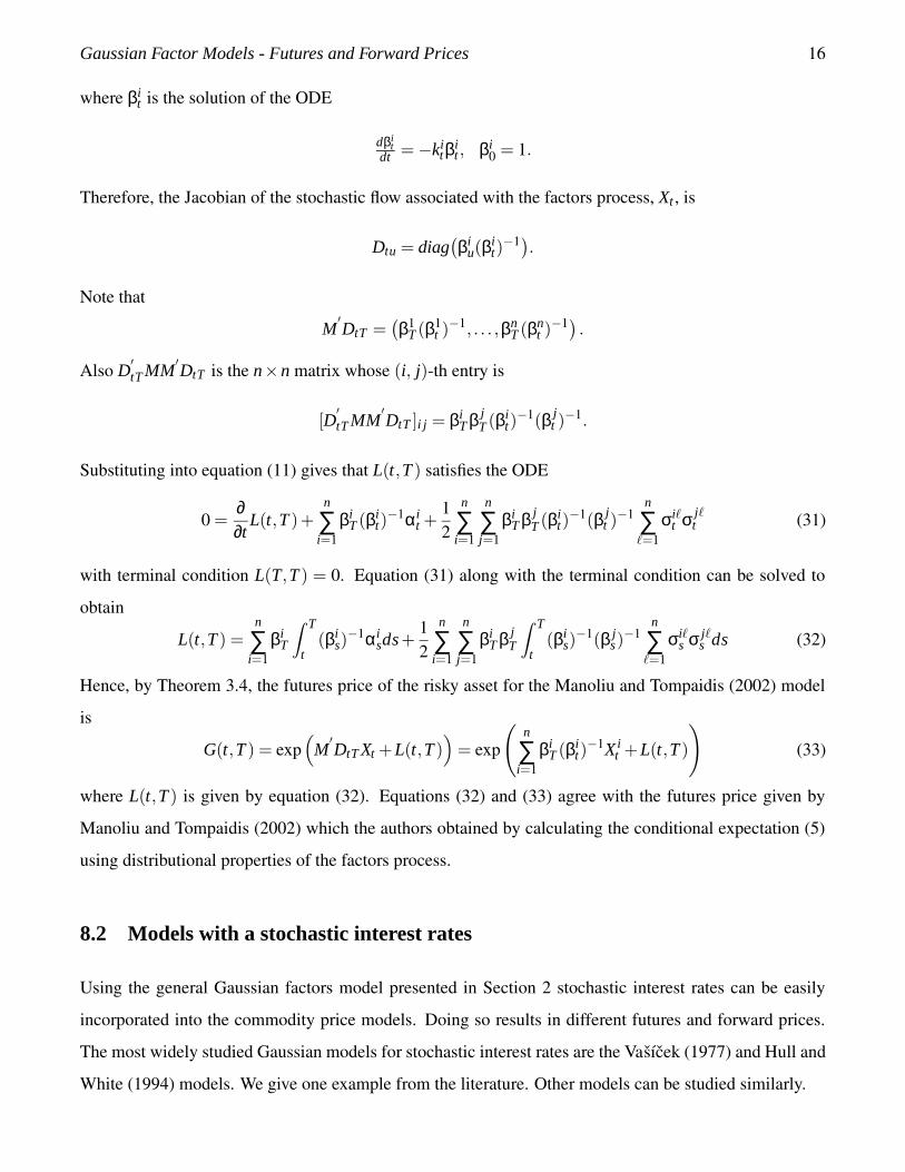
Substituting into equation (11) gives that L(t,T ) satisfies the ODE
0 =∂∂t
L(t,T )+n
∑i=1
βiT (βi
t)−1αi
t +12
n
∑i=1
n
∑j=1
βiT β j
T (βit)−1(β j
t )−1
n
∑=1
σi`t σ j`
t (31)
with terminal condition L(T,T ) = 0. Equation (31) along with the terminal condition can be solved to
obtain
L(t,T ) =n
∑i=1
βiT
Z T
t(βi
s)−1αi
sds+12
n
∑i=1
n
∑j=1
βiT β j
T
Z T
t(βi
s)−1(β j
s)−1
n
∑=1
σi`s σ j`
s ds (32)
Hence, by Theorem 3.4, the futures price of the risky asset for the Manoliu and Tompaidis (2002) model
is
G(t,T ) = exp(
M′DtT Xt +L(t,T )
)
= exp(
n
∑i=1
βiT (βi
t)−1X i
t +L(t,T )
)
(33)
where L(t,T ) is given by equation (32). Equations (32) and (33) agree with the futures price given by
Manoliu and Tompaidis (2002) which the authors obtained by calculating the conditional expectation (5)
using distributional properties of the factors process.
8.2 Models with a stochastic interest rates
Using the general Gaussian factors model presented in Section 2 stochastic interest rates can be easily
incorporated into the commodity price models. Doing so results in different futures and forward prices.
The most widely studied Gaussian models for stochastic interest rates are the Vasıcek (1977) and Hull and
White (1994) models. We give one example from the literature. Other models can be studied similarly.

Gaussian Factor Models - Futures and Forward Prices 17
8.2.1 Schwartz (1997): Model 3 (Three-factor model)
We shall derive the futures price and forward price for a three-factor commodity market model considered
by Schwartz (1997) which includes stochastic interest rates and stochastic dividends. Schwartz (1997)
considers the dynamics
dSt = (rt −δt)Stdt +σ1StdB(1)t (34)
dδt = κ(α−δt)]dt +σ2dB(2)t (35)
drt = a(m− rt)dt +σ3dB(3)t (36)
with d⟨
B(1),B(2)⟩
t= ρ12dt, d
⟨
B(1),B(3)⟩
t= ρ13dt, and d
⟨
B(2),B(3)⟩
t= ρ23dt. Schwartz (1997) used
the Kalman filter and maximum likelihood parameter estimation to study futures contracts on oil, copper,
and gold.
Since our discussions have assumed standard Brownian motion (ρ12 = ρ23 = ρ13 = 0) we consider an
equivalent formulation of the model. That is, suppose Xt = (logSt ,δt ,rt)′ satisfies equation (1) where
Bt = (B(1)t ,B(2)
t ,B(3)t )
′ is a standard Brownian motion taking values in R3,
γt =
−12σ2
1
κα
am
, At =
0 −1 1
0 −κ 0
0 0 −a
,
and
σt =
σ1 0 0
σ2ρ12 σ2
√
1−ρ212 0
σ3ρ13σ3(ρ23−ρ12ρ13)√
1−ρ212
σ3
√
1− ρ213−2ρ12ρ13ρ23+ρ2
231−ρ2
12
.
We consider Xt as our underlying factor in the context of the general Gaussian model. Then with R = e3 ∈R3, M = e1 ∈ R3, N = e2 ∈ R3, k = 0, h = 0, and l = 0 in Assumption 2.2 the market model is equivalent
to the formulation given by Schwartz (1997), i.e., equations (34)-(36).
The Jacobian of the stochastic flow associated with Xt is
Dtu =
1 − 1κ
(
1− e−κ(T−t))
1a
(
1− e−a(T−t))
0 e−κ(T−t) 0
0 0 e−a(T−t)
.
Note that
M′DtT =
(
1 − 1κ
(
1− e−κ(T−t))
1a
(
1− e−a(T−t)))
.

Gaussian Factor Models - Futures and Forward Prices 18
Substituting into equation (11) gives that L(t,T ) satisfies the ODE
0 =∂∂t
L(t,T )− [κα+σ1σ2ρ12]
(
1− e−κ(T−t))
κ+[am+σ1σ3ρ13]
(
1− e−a(T−t))
a(37)
+12
σ22
κ2
(
1− e−κ(T−t))2
+12
σ23
a2
(
1− e−a(T−t))2
−σ2σ3ρ23
(
1− e−κ(T−t))(
1− e−a(T−t))
κa
with terminal condition L(T,T ) = 0. Equation (37) along with the terminal condition can be solved to
obtain
L(t,T ) = (κα+σ1σ2ρ12)
[
(1− e−κ(T−t))−κ(T − t)κ2
]
− (ma+σ1σ3ρ13)
[
(1− e−a(T−t))−a(T − t)a2
]
− σ22
[
4(1− e−κ(T−t))− (1− e−2κ(T−t))−2κ(T − t)4κ3
]
− σ23
[
4(1− e−a(T−t))− (1− e−2a(T−t))−2a(T − t)4a3
]
(38)
+σ2σ3ρ23
κa
(
1− e−κ(T−t))
κ+
(
1− e−a(T−t))
a−
(
1− e−(κ+a)(T−t))
(κ+a)− (T − t)
.
Hence, by Theorem 3.4, the futures price of the risky asset for the three-factor model of Schwartz (1997)
is
G(t,T ) = exp(
M′DtT Xt +L(t,T )
)
= St exp(
−(1− e−κ(T−t))
κδt +
(1− e−a(T−t))
art +L(t,T )
)
(39)
where L(t,T ) is given by equation (38). Equations (38) and (39) agree with the futures price which can be
obtained from the results given by Schwartz (1997). The results presented by Schwartz (1997) are stated
to be verifiable by substitution into the PDE for the futures price.
Substituting into equation (27) gives that C(t,T ) satisfies the ODE
0 =∂∂t
C(t,T )−α(
1− e−κ(T−t))
+m(
1− e−a(T−t))
(40)
+1κ2 σ2
2
(
1− e−κ(T−t))2
− 1a2 σ2
3
(
1− e−a(T−t))2
− σ1σ2ρ12κ
(
1− e−κ(T−t))
with terminal condition C(T,T ) = 0. Equation (40) along with the terminal condition can be solved to
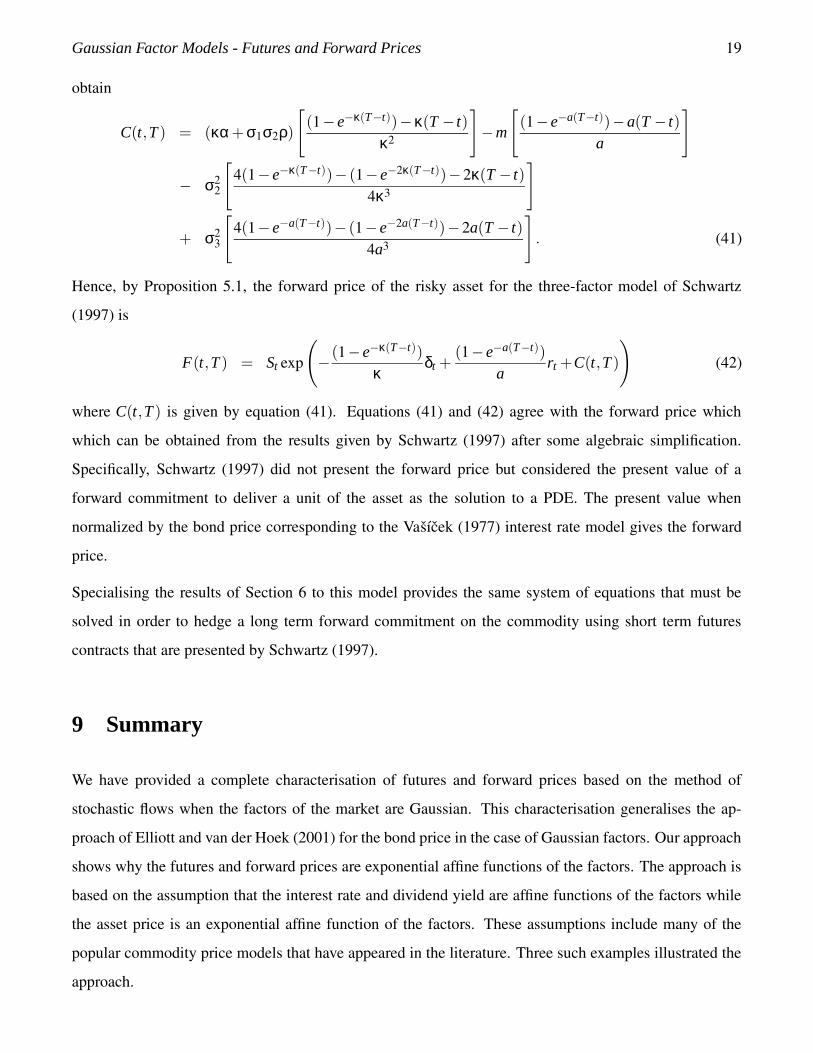
Gaussian Factor Models - Futures and Forward Prices 19
obtain
C(t,T ) = (κα+σ1σ2ρ)
[
(1− e−κ(T−t))−κ(T − t)κ2
]
−m
[
(1− e−a(T−t))−a(T − t)a
]
− σ22
[
4(1− e−κ(T−t))− (1− e−2κ(T−t))−2κ(T − t)4κ3
]
+ σ23
[
4(1− e−a(T−t))− (1− e−2a(T−t))−2a(T − t)4a3
]
. (41)
Hence, by Proposition 5.1, the forward price of the risky asset for the three-factor model of Schwartz
(1997) is
F(t,T ) = St exp(
−(1− e−κ(T−t))
κδt +
(1− e−a(T−t))
art +C(t,T )
)
(42)
where C(t,T ) is given by equation (41). Equations (41) and (42) agree with the forward price which
which can be obtained from the results given by Schwartz (1997) after some algebraic simplification.
Specifically, Schwartz (1997) did not present the forward price but considered the present value of a
forward commitment to deliver a unit of the asset as the solution to a PDE. The present value when
normalized by the bond price corresponding to the Vasıcek (1977) interest rate model gives the forward
price.
Specialising the results of Section 6 to this model provides the same system of equations that must be
solved in order to hedge a long term forward commitment on the commodity using short term futures
contracts that are presented by Schwartz (1997).
9 Summary
We have provided a complete characterisation of futures and forward prices based on the method of
stochastic flows when the factors of the market are Gaussian. This characterisation generalises the ap-
proach of Elliott and van der Hoek (2001) for the bond price in the case of Gaussian factors. Our approach
shows why the futures and forward prices are exponential affine functions of the factors. The approach is
based on the assumption that the interest rate and dividend yield are affine functions of the factors while
the asset price is an exponential affine function of the factors. These assumptions include many of the
popular commodity price models that have appeared in the literature. Three such examples illustrated the
approach.
Gaussian Factor Models - Futures and Forward Prices 20
References
Babbs, S. H. and Nowman, K. B. (1999). Kalman filtering of generalized Vasicek term structure models,
Journal of financial and quantitative analysis 34(1): 115–130.
Bjerksund, P. (1991). Contingent claim evaluation when the convenience yield is stochastic: analytical
results. Working paper, Norwegian School of Economics and Business Administration.
Bjork, T. and Landen, C. (2002). On the term structure of futures and forward prices, Mathematical
finance—Bachelier Congress, 2000 (Paris), Springer Finance, Springer, Berlin, pp. 111–149.
Cortazar, G. and Schwartz, E. (1994). The evaluation of commodity contingent claims, J. Derivatives
1: 27–39.
Cox, J., Ingersoll, J. and Ross, S. (1981). The relation between forward and futures prices, Journal of
Financial Economics 9: 321–346.
Cox, J., Ingersoll, J. and Ross, S. (1985). A theory of the term structure of interest rates, Econometrica
53: 385–408.
Duffie, D. and Kan, R. (1996). A yield-factor model of interest rates, Math. Finance 6(4): 379–406.
Elliott, R. J. and Hyndman, C. B. (2006). Parameter estimation in commodity markets: a filtering ap-
proach. Journal of Economic Dynamics and Control, to appear.
Elliott, R. J. and van der Hoek, J. (2001). Stochastic flows and the forward measure, Finance Stoch.
5: 511–525.
Friedman, A. (1975). Stochastic differential equations and applications., Academic Press, New York.
Gibson, R. and Schwartz, E. S. (1990). Stochastic convenience yield and the pricing of oil contingent
claims, Journal of Finance XLV(3): 959–976.
Heath, D., Jarrow, R. and Morton, A. (1992). Bond pricing and the term structure of interest rates: A new
methodology for contingent claims valuation, Econometrica 60(1): 77–105.
Hull, J. C. (2002). Futures, options, and other derivatives, fifth edn, Prentice-Hall.
Hull, J. C. and White, A. (1994). Numerical procedures for implementing term structure models ii, Journal
of Derivatives 2: 37–48.

Gaussian Factor Models - Futures and Forward Prices 21
Hyndman, C. B. (2005). Affine futures and forward prices, PhD thesis, University of Waterloo, Canada.
Karatzas, I. and Shreve, S. E. (1991). Brownian Motion and Stochastic Calculus, second edn, Springer-
Verlag, New York.
Karatzas, I. and Shreve, S. E. (1998). Methods of mathematical finance, Spinger-Verlag, New York.
Levendorskiı, S. (2004). Consistency conditions for affine term structure models, Stochastic Process.
Appl. 109(2): 225–261.
Manoliu, M. and Tompaidis, S. (2002). Energy futures prices: term structure models with Kalman filter
estimation, Applied Mathematical Finance 9: 21–43.
Miltersen, K. R. and Schwartz, E. S. (1998). Pricing of options on commodity futures with stochastic
term structures of convenience yields and interest rates, Journal of Financial and Quantitative Analysis
33(1): 33–59.
Protter, P. (1990). Stochastic integration and differential equations: a new approach, Vol. 21 of Applica-
tions of Mathematics, Springer-Verlag, New York.
Ribeiro, D. and Hodges, S. (2004). A two-factor model for commodity prices and futures valuation.
Preprint.
Schroder, M. (1999). Changes of numeraire for pricing, futures, forwards, and options, The Review of
Financial Studies 12(5): 1143–1163.
Schwartz, E. S. (1997). The stochastic behaviour of commodity prices: Implications for valuation and
hedging, Journal of Finance LII(3): 923–973.
Schwartz, E. S. (1998). Valuing long-term commodity assets, Financial Management 27(1): 57–66.
Schwartz, E. S. and Smith, J. E. (2000). Short-term variations and long-term dynamics in commodity
prices, Management Science 46(7): 893–911.
Vasıcek, O. (1977). An equilibrium characterization of the term structure, Journal of Financial Economics
5: 177–188.
Yan, X. (2002). Valuation of commodity derivatives in a new multi-factor model, Review of Derivatives
Research 5: 251–271.