Embed Size (px)
Citation preview
8/18/2019 Gasmi Cost Proxy Models
http://slidepdf.com/reader/full/gasmi-cost-proxy-models 1/318
Cost Proxy Models and Telecommunications Policy
A New Empirical Approach to Regulation
F. Gasmi
Institut D’Economie Industrielle, Universit de Toulouse I, France
D.M. Kennet
George Washington University, Washington DC, USA
J.J. Laffont
Institut D’Economie Industrielle, Universit de Toulouse I, France
W.W. Sharkey
Federal Communications Commission, Washington DC, USA
August 2001

8/18/2019 Gasmi Cost Proxy Models
http://slidepdf.com/reader/full/gasmi-cost-proxy-models 2/318
2
to Aaron, Ali, Bndicte, Benjamin, Bertrand, Ccile, Charlotte, Michael, Nadine and Re-
becca
8/18/2019 Gasmi Cost Proxy Models
http://slidepdf.com/reader/full/gasmi-cost-proxy-models 3/318
Contents
Preface 9
1 Introduction 13
1.1 The Need for Regulation in Telecommunications . . . . . . . . . . . . . . . 13
1.2 The Historical Evolution of Practical Regulation . . . . . . . . . . . . . . . 16
1.3 The New Theory of Regulation . . . . . . . . . . . . . . . . . . . . . . . . 19
1.4 Econometrics of Regulation . . . . . . . . . . . . . . . . . . . . . . . . . . 21
1.5 Cost Proxy Models . . . . . . . . . . . . . . . . . . . . . . . . . . . . . . . 24
1.6 A New Empirical Approach to Regulation . . . . . . . . . . . . . . . . . . 26
2 The Local Exchange Cost Optimization Model (LECOM) 33
2.1 Introduction . . . . . . . . . . . . . . . . . . . . . . . . . . . . . . . . . . . 33
2.2 The Local Exchange Network: An Overview . . . . . . . . . . . . . . . . . 35
2.3 Technological Foundations of LECOM . . . . . . . . . . . . . . . . . . . . 38
2.3.1 The Distribution Plant . . . . . . . . . . . . . . . . . . . . . . . . . 38
2.3.2 The Feeder Plant . . . . . . . . . . . . . . . . . . . . . . . . . . . . 42
2.3.3 Switching . . . . . . . . . . . . . . . . . . . . . . . . . . . . . . . . 43
2.3.4 The Interoffice Plant . . . . . . . . . . . . . . . . . . . . . . . . . . 45
3
8/18/2019 Gasmi Cost Proxy Models
http://slidepdf.com/reader/full/gasmi-cost-proxy-models 4/318
4 CONTENTS
2.4 Building an Optimal Network: Economic Trade-Offs Modeled... . . . . . . 46
2.5 Total Cost and Optimization . . . . . . . . . . . . . . . . . . . . . . . . . . 48
2.6 From LECOM Simulations to a LECOM Cost Function . . . . . . . . . . . 53
3 The Use of LECOM under Complete Information 63
3.1 Introduction . . . . . . . . . . . . . . . . . . . . . . . . . . . . . . . . . . . 63
3.2 Data Problems Encountered in Prior Studies . . . . . . . . . . . . . . . . . 65
3.3 Using the LECOM Model for Subadditivity Calculations . . . . . . . . . . 68
3.4 Empirical Results . . . . . . . . . . . . . . . . . . . . . . . . . . . . . . . . 70
3.4.1 Measuring Economies of Scope . . . . . . . . . . . . . . . . . . . . . 70
3.4.2 Economies of Scope in Switched Services . . . . . . . . . . . . . . . 76
3.5 Conclusion . . . . . . . . . . . . . . . . . . . . . . . . . . . . . . . . . . . . 77
4 Regulation under Incomplete Information 83
4.1 Introduction . . . . . . . . . . . . . . . . . . . . . . . . . . . . . . . . . . . 83
4.2 The Model . . . . . . . . . . . . . . . . . . . . . . . . . . . . . . . . . . . . 85
4.3 Optimal Regulation under Incomplete Information... . . . . . . . . . . . . . 87
4.4 Optimal Regulation without Cost Observability . . . . . . . . . . . . . . . 91
4.5 Price-Cap Regulation . . . . . . . . . . . . . . . . . . . . . . . . . . . . . . 92
4.6 Cost-Plus Regulation . . . . . . . . . . . . . . . . . . . . . . . . . . . . . . 95
4.7 Remark . . . . . . . . . . . . . . . . . . . . . . . . . . . . . . . . . . . . . 96
5 The Natural Monopoly Test 101
5.1 Introduction . . . . . . . . . . . . . . . . . . . . . . . . . . . . . . . . . . . 101
8/18/2019 Gasmi Cost Proxy Models
http://slidepdf.com/reader/full/gasmi-cost-proxy-models 5/318
CONTENTS 5
5.2 Theoretical Framework . . . . . . . . . . . . . . . . . . . . . . . . . . . . . 105
5.3 Empirical Methodology . . . . . . . . . . . . . . . . . . . . . . . . . . . . . 110
5.3.1 Simulations of The Engineering Process Cost Model LECOM . . . . 111
5.3.2 Market Structure-Specific Cost Functions . . . . . . . . . . . . . . . 114
5.3.3 Interconnection Costs . . . . . . . . . . . . . . . . . . . . . . . . . . 116
5.3.4 Calibration of Demand and Disutility . . . . . . . . . . . . . . . . . 119
5.4 Empirical Results . . . . . . . . . . . . . . . . . . . . . . . . . . . . . . . . 120
5.4.1 Case I: Usage as Output . . . . . . . . . . . . . . . . . . . . . . . . 121
5.4.2 Case II: Access as Output . . . . . . . . . . . . . . . . . . . . . . . 125
5.5 Conclusion . . . . . . . . . . . . . . . . . . . . . . . . . . . . . . . . . . . . 130
6 Optimal Regulation of a Natural Monopoly 139
6.1 Introduction . . . . . . . . . . . . . . . . . . . . . . . . . . . . . . . . . . . 139
6.2 The Optimal Regulatory Mechanism: Theory . . . . . . . . . . . . . . . . 141
6.3 The Local Exchange Cost Function, Welfare and Regulatory: . . . . . . . . 143
6.4 The Optimal Regulatory Mechanism: Empirical Evaluation . . . . . . . . . 147
6.5 Implications . . . . . . . . . . . . . . . . . . . . . . . . . . . . . . . . . . . 152
6.5.1 Incentives and Pricing . . . . . . . . . . . . . . . . . . . . . . . . . 152
6.5.2 Implementation of Optimal Regulation . . . . . . . . . . . . . . . . 155
6.6 Using an Alternative Disutility of Effort Function . . . . . . . . . . . . . . 161
6.7 Conclusion . . . . . . . . . . . . . . . . . . . . . . . . . . . . . . . . . . . . 163
7 Comparison of Performance... 171
8/18/2019 Gasmi Cost Proxy Models
http://slidepdf.com/reader/full/gasmi-cost-proxy-models 6/318
6 CONTENTS
7.1 Introduction . . . . . . . . . . . . . . . . . . . . . . . . . . . . . . . . . . . 171
7.2 Alternative Regulatory Regimes . . . . . . . . . . . . . . . . . . . . . . . . 173
7.3 Overview of The Results . . . . . . . . . . . . . . . . . . . . . . . . . . . . 177
7.4 Comparisons and Implications . . . . . . . . . . . . . . . . . . . . . . . . . 185
7.4.1 Relative Performance . . . . . . . . . . . . . . . . . . . . . . . . . . 185
7.4.2 Redistributive Consequences . . . . . . . . . . . . . . . . . . . . . . 187
7.4.3 Effect of The Cost of Public Funds . . . . . . . . . . . . . . . . . . 192
7.5 Conclusion . . . . . . . . . . . . . . . . . . . . . . . . . . . . . . . . . . . . 194
8 Universal Service 199
8.1 Introduction . . . . . . . . . . . . . . . . . . . . . . . . . . . . . . . . . . . 199
8.2 The Theoretical Alternatives . . . . . . . . . . . . . . . . . . . . . . . . . . 201
8.3 Empirical Procedure . . . . . . . . . . . . . . . . . . . . . . . . . . . . . . 209
8.4 Empirical Results . . . . . . . . . . . . . . . . . . . . . . . . . . . . . . . . 211
8.4.1 Technological Efficiency . . . . . . . . . . . . . . . . . . . . . . . . 211
8.4.2 Universal Service Obligation and Budget Balance . . . . . . . . . . 213
8.4.3 Implicit and Explicit Taxation of The Urban Sector . . . . . . . . . 215
8.4.4 Impact of Incomplete Information . . . . . . . . . . . . . . . . . . . 217
8.5 Conclusion . . . . . . . . . . . . . . . . . . . . . . . . . . . . . . . . . . . . 218
9 Strategic Cross-Subsidies and Vertical Integration 227
9.1 Introduction . . . . . . . . . . . . . . . . . . . . . . . . . . . . . . . . . . . 227
9.2 Size of Cross-Subsidies Due to Allocation of Common Costs . . . . . . . . 228
8/18/2019 Gasmi Cost Proxy Models
http://slidepdf.com/reader/full/gasmi-cost-proxy-models 7/318
CONTENTS 7
9.3 Size of Effort Allocation Cross-Subsidies . . . . . . . . . . . . . . . . . . . 231
9.4 Strategic Cross-Subsidies Through Effort... . . . . . . . . . . . . . . . . . . 233
9.4.1 The Cost of Effort Channel . . . . . . . . . . . . . . . . . . . . . . 233
9.4.2 The Cost of Production Channel . . . . . . . . . . . . . . . . . . . 235
9.5 Empirical Results . . . . . . . . . . . . . . . . . . . . . . . . . . . . . . . . 237
9.5.1 Simulation of LECOM: Basic vs Enhanced Services . . . . . . . . . 237
9.5.2 Accounting and Strategic Cross-Subsidies . . . . . . . . . . . . . . . 241
9.6 Conclusion . . . . . . . . . . . . . . . . . . . . . . . . . . . . . . . . . . . . 248
10 Conclusion 253
10.1 What Have We Learned? . . . . . . . . . . . . . . . . . . . . . . . . . . . . 254
10.1.1 Implications for incentive regulation and telecommunications policy 254
10.1.2 Lessons for the use of proxy models in empirical research . . . . . . 258
10.2 Directions for Improvements in Our Approach . . . . . . . . . . . . . . . . 261
10.3 Some Issues Not Addressed in Our Analysis and Suggestions . . . . . . . . 264
References 271
Appendix A 281
A.1 The Natural Monopoly Test (Chapter 5) . . . . . . . . . . . . . . . . . . . . 281
A.2 Optimal Regulation of a Natural Monopoly (Chapter 6) . . . . . . . . . . . 282
A.3 Universal Service (Chapter 8) . . . . . . . . . . . . . . . . . . . . . . . . . . 283
A.4 Strategic Cross-Subsidies and Vertical Integration (Chapter 9) . . . . . . . . 285
A.5 Preparation of LECOM Cost Data . . . . . . . . . . . . . . . . . . . . . . . 290
8/18/2019 Gasmi Cost Proxy Models
http://slidepdf.com/reader/full/gasmi-cost-proxy-models 8/318
8 CONTENTS
A.6 A Guide to The Mathematica Analysis . . . . . . . . . . . . . . . . . . . . . 297
A.7 Contents of the CDRom . . . . . . . . . . . . . . . . . . . . . . . . . . . . . 299
Appendix B 303
B.1 The Hybrid Cost Proxy Model (HCPM) . . . . . . . . . . . . . . . . . . . . 303
B.2 International Applications of HCPM . . . . . . . . . . . . . . . . . . . . . . 310
Argentina . . . . . . . . . . . . . . . . . . . . . . . . . . . . . . . . . . . . 311
Portugal . . . . . . . . . . . . . . . . . . . . . . . . . . . . . . . . . . . . . 313
8/18/2019 Gasmi Cost Proxy Models
http://slidepdf.com/reader/full/gasmi-cost-proxy-models 9/318
Preface
The research reported in this book was started during the academic year 1994-1995 when
Bill Sharkey visited the Institut D’Economie Industrielle in Toulouse. The desire to bring
modern industrial economics to the data was already quite strong for Farid Gasmi and
Jean-Jacques Laffont. After some empirical work on oligopolistic markets (Gasmi, Laffont
and Vuong, 1992), auctions (Laffont, Ossard and Vuong, 1995) and contracts (Laffont and
Matoussi, 1995), the challenge to confront the new economics of regulation with the real
world seemed particularly daunting. First, incentive regulation was in place only recently.
Second, data related to these new regulatory policies were very scarce. Third, and thisis particularly true for the case of Telecommunications, the need to focus on forward-
looking technologies in an industry so quickly evolving limited the power of classical
economic methods. We only had the small experience of some simulations on calibrated
models (Gasmi, Ivaldi and Laffont, 1994) following Schmalensee (1989). Bill came to
Toulouse with the desire to invest in empirical approaches to cost studies and industry
structure. At that time, the LECOM cost engineering model, developed by Gabel and
Kennet (1991, 1994), had already been used to investigate economies of scale in local
telecommunications. As a consequence of the debate taking place at the state level in the
U.S., the National Regulatory Research Institute (the research arm of state regulators),
had funded the original version of LECOM through a grant to David Gabel and Mark
Kennet. Bill, who was about to join the Federal Communications Commission, was also
interested in using this type of instrument for the debates about regulatory intervention
at the national level.
The project started with the idea of simulating with LECOM, cost functions which
9

8/18/2019 Gasmi Cost Proxy Models
http://slidepdf.com/reader/full/gasmi-cost-proxy-models 10/318
10 PREFACE
would incorporate moral hazard and adversse selection variables. Endowed with this
instrument, we could then review some of the major policy issues concerning the localtelecommunications industry, including the natural monopoly question, the comparison of
various regulatory mechanisms, the universal service obligation and cross-subsidies, within
the intellectual framework of the new regulatory economics developed in the eighties and
the nineties. All along, Mark Kennet was very helpful in the manipulation of the LECOM
model in order to customize it to our specific simulation needs and later joined the group
to synthesize what we had learned in this book.
Despite the resources put together in our team of four, this was insufficient to realize
a study which could be directly policy relevant. The work presented here is largely
methodological and aimed at showing that a combination of cost engineering models
with econometrics and simulations can help the policy discussions of some of the major
issues of regulation. Precise answers for particular industries and countries or regions
would definitely require more inputs. We, however, hope to convince the reader that this
approach has some value and to stimulate further research along the lines followed in this
book. For academic use, we have provided a CD Rom which will enable researchers to
extend our efforts and further develop the paradigm.
We are grateful to MIT Press for publishing this book and to Richard Schmalensee
for welcoming this volume in the series he is editing. Many thanks to Daniel Benitez,
Srinagesh Padmanabhan and our colleagues in Toulouse for useful comments on an earlier
draft. We would also like to thank David Gabel, who graciously allowed us to include
work to which he has greatly contributed. We warmly thank Christelle Fauchi for skillfully
typing the manuscript. Finally, Farid Gasmi and Jean-Jacques Laffont thank France
Tlcom for financial support without which the undertaking of this work would have never
been possible.
Farid Gasmi, Jean-Jacques Laffont, Toulouse
Mark Kennet, Bill Sharkey, Washington, DC

8/18/2019 Gasmi Cost Proxy Models
http://slidepdf.com/reader/full/gasmi-cost-proxy-models 11/318
11
August 31, 2001

8/18/2019 Gasmi Cost Proxy Models
http://slidepdf.com/reader/full/gasmi-cost-proxy-models 12/318
12 PREFACE
8/18/2019 Gasmi Cost Proxy Models
http://slidepdf.com/reader/full/gasmi-cost-proxy-models 13/318
Chapter 1
Introduction
1.1 The Need for Regulation in Telecommunications
The telecommunications industry, as every economist and industry observer knows, is
an industry in transition. Once regarded as a classic example of a natural monopoly,
the industry today defies easy characterization. A portion of the industry representing
traditional voice communication between parties in widely separated communities - the so-
called “long distance” sector of the industry - has been successfully opened to competition
in many countries, and few would dispute that the market for these services is highly
competitive, at least for now. On the other hand, the local exchange portion of the
industry, though also opened to competitive entry in recent years, has seen relatively
little actual entry, except in the portion of the market serving very high volume users.
Moreover, the adoption of digital transmission and switching technologies has blurred the
distinction between traditional voice communication and the transmission of video and
data messages. The same network can carry all forms of information efficiently in a digital
format, although there remain important regulatory distinctions between the packet only
networks, which include the internet backbones, and circuit switched networks, which
continue to provide most of the voice grade services.
Technology and regulation are the defining characteristics of telecommunications. Reg-
ulation of telecommunications was generally regarded as necessary because portions of the
13
8/18/2019 Gasmi Cost Proxy Models
http://slidepdf.com/reader/full/gasmi-cost-proxy-models 14/318
14 CHAPTER 1. INTRODUCTION
industry have the technological characteristics of natural monopoly. In part, the defini-
tion of natural monopoly is a statement about the technology of the industry, or moreprecisely about the cost function. It is often said that an industry is a natural monopoly if
a single firm can produce the industry output at lower cost than any alternative collection
of two or more firms.1 This definition, however, raises new questions about the meaning
of cost. How are the costs of a single firm in an industry to be measured? Do these costs
depend on the nature of regulation in the industry? Similarly, one must ask what are
the costs of the multifirm alternative to a regulated natural monopoly? These costs will
clearly depend on the nature of regulation that may continue to exist in the market as
well as on the strategic behavior of the firms which seek to maximize their profits subject
to regulatory constraints and the behavior of rival firms.
In the telecommunications industry, regulation clearly has a significant impact on the
cost of any firm subject to that regulation. A regulator must design and oversee the
mechanism by which the regulated firm is allowed to recover its costs. A regulator may
allow open entry in certain markets served by a regulated firm, while restricting entry in
other markets. A regulator may impose structural or accounting constraints on a regulated
firm which serves markets with differing degrees of competition. A regulator may even
require a regulated firm to serve an unprofitable segment of the market in the interest of
satisfying a “universal service” objective. Similarly, in a multifirm telecommunications
market, both accounting or structural constraints and a universal service obligation may
be imposed on one or more firms in the market. These factors will clearly affect the
market equilibrium and the realization of cost for each firm in the market.
An additional factor in evaluating the cost structure of a multifirm market for telecom-
munications services is the set of rules governing the interconnection of carriers. In the
absence of any such rules, large networks may refuse to interconnect with smaller net-
works, and this possibility may itself create a tendency to natural monopoly, even in the
absence of other cost based factors favoring single firm production. Proper interconnec-
tions call for regulatory intervention.2 The interconnection of networks, however, is itself

8/18/2019 Gasmi Cost Proxy Models
http://slidepdf.com/reader/full/gasmi-cost-proxy-models 15/318
1.1. THE NEED FOR REGULATION IN TELECOMMUNICATIONS 15
costly, and the nature of the rules governing interconnection may impose additional costs
on firms in the market, if they create incentives for the inefficient deployment of networkfacilities.3
Finally, an empirical evaluation of telecommunications policies must be concerned
with the actual measurement of a cost function for telecommunications firms. Since
it is clearly recognized that only the forward-looking costs are relevant to most policy
issues in telecommunications, how can the relevant cost function be estimated? The
same regulators that may impose conditions on regulated firms to advance various socialobjectives may also wish to evaluate alternative regulatory policies, including possibly the
partial or total deregulation of the industry. In most cases, historical time series data will
not be adequate for an econometric investigation of cost, unless the policy change has
already been implemented and the evaluation is retrospective. Cross sectional analysis is
more likely to be useful, but only if there exist other regulatory jurisdictions that have
previously implemented a similar policy change.
We see little value in a pedantic reformulation of the definition of natural monopoly
which incorporates the above factors. It is sufficient to observe that both technology and
market forces can lead to situations, in telecommunications and in similarly structured
industries, in which regulation leads to higher social welfare than the unregulated alterna-
tive. Broadly speaking, the purpose of this book is to examine many of the issues raised
above concerning natural monopoly, and the need for regulation of telecommunications,
in an empirical setting. Our analysis is based on the insights of the “new theory of reg-
ulation” which we outline in Section 1.3 below and develop more fully in Chapter 4. An
important, indeed crucial, tool for this analysis is the use of a computer based cost proxy
model as a descriptor of the underlying telecommunications cost or production function.
In the remainder of this introductory chapter we present the basic ingredients of what we
believe to be a new and promising empirical approach to regulation.
Section 1.2 recaps the recent historical evolution of regulation in telecommunications.
The so-called New Theory of Regulation based on a proper recognition of the regulators’
8/18/2019 Gasmi Cost Proxy Models
http://slidepdf.com/reader/full/gasmi-cost-proxy-models 16/318
16 CHAPTER 1. INTRODUCTION
information constraints is introduced in Section 1.3. The difficulties faced by the econo-
metrics of regulated industries are discussed in Section 1.4. The cost proxy models whichprovide an alternative to econometric approaches of costs are described in Section 1.5.
Section 1.6 puts together all these elements to propose the new empirical approach to
regulation which is the topic of this book.
1.2 The Historical Evolution of Practical Regulation
Alexander Graham Bell was granted patents in 1876 and 1877 for “improvements in
telegraphy” which provided the basic ingredients for the new industry of voice telephone
service. Regulation of telephone service began in 1879, when Connecticut and Missouri
became the first states to regulate telephone companies as public utilities. By 1920, all
but three states had established public utility commissions with jurisdiction over rates
and practices of telephone companies.4 After the expiration in 1894 of the basic Bell
patents, there followed a period of entry by independent telephone companies and in-
tense competition between the Bell companies and independents for local services. The
Bell companies, however, maintained the only viable technology for long distance com-
munications between subscribers in different cities through their subsidiary, the American
Telephone and Telegraph Company. In the early years of the 20th Century, many of these
independent companies were forced to merge with A.T.&T., since that company pursued
an aggressive pricing policy and generally refused to interconnect with the independent
companies.
The difficulty of duplicating facilities at the local level, and the refusal of the Bell com-
panies to interconnect led to significant pressure to impose regulation at the federal level.
Rather than opposing these calls for regulation, Theodore Vail, the president of A.T.&.T.,
choose to embrace regulation. In 1913 the company voluntarily agreed to interconnect
with all remaining independents and to refrain from acquiring any more independent
companies. The resulting “Bell System” was initially regulated under the jurisdiction of
the Interstate Commerce Commission. In 1934, the U.S. Congress passed the Commu-
8/18/2019 Gasmi Cost Proxy Models
http://slidepdf.com/reader/full/gasmi-cost-proxy-models 17/318
1.2. THE HISTORICAL EVOLUTION OF PRACTICAL REGULATION 17
nications Act, creating the Federal Communications Commission with authority over all
interstate rates and activities of the Bell System.5
At both the state and federal level, regulation followed traditional public utility pricing
principles, based on the idea of a “fair rate of return” on the utility’s rate base.6 Under
rate of return regulation, the firm essentially reports its costs to the regulator, and subject
to auditing of these reports, the regulator guarantees that the firm is fully reimbursed for
its costs and is allowed to earn a normal rate of return on the firm’s capital assets. It is
now well known that this form of regulation leads to a number of perverse incentives forthe regulated firm. The firm may have an incentive to over-invest in capital inputs relative
to labor or other variable inputs as long as the allowed rate of return exceeds the firm’s
cost of capital.7 Since the firm itself is likely to have more complete information about
its cost function than the regulator, the firm may have weak or non-existent incentives
to engage in cost-reducing activities.8 Finally, under rate of return regulation, the firm
may have powerful incentives to engage in cost shifting between competitive and non-
competitive activities to the extent that these actions cannot be easily detected by the
regulator.
For the above reasons, the costs of a firm operating under rate of return regulation
are likely to be significantly different from those of a similarly situated firm operating in
an unregulated market. Based on this observation, one could conclude that, at least in
principle, an unregulated firm might perform better than a regulated firm in some poten-
tial natural monopoly markets. This result would occur if the various price distortions
associated with the market power of the unregulated firm were judged to be less costly
than the inefficiencies induced by the regulatory process. There are, however, alterna-
tive regulatory policies that should also be evaluated before assessing the proper role of
regulation generally. In fact, a particular alternative, known as price-cap regulation, has
been widely adopted in the telecommunications industry in recent years since it gives the
regulated firm good incentives to produce outputs in a cost-minimizing manner, while
allowing the regulator to maintain some control over the firm’s prices.

8/18/2019 Gasmi Cost Proxy Models
http://slidepdf.com/reader/full/gasmi-cost-proxy-models 18/318
18 CHAPTER 1. INTRODUCTION
Price cap regulation was first suggested by Littlechild (1983) in the United Kingdom
and was later adopted by the FCC and many state regulatory commissions in the UnitedStates.9 The generally favorable analysis of price-cap regulation by economists was based
on a growing understanding of the role of incentives in the design of good regulatory
mechanisms. Price caps are considered a good, or “high-powered” regulatory instrument
since they allow the firm to capture the full benefits of any-cost reducing activities that it
chooses to pursue. Since firms are generally much better informed than regulators about
the nature of the cost or production function, this delegation of authority to the firm can
result in significant cost savings. However, the same informational asymmetry requires
that the regulator allow the firm to retain some monopoly profits in all but the most
adverse circumstances. The trade-off between cost reduction and rents is fundamental
to the modern approach to incentive regulation, and will be the subject of much of this
book.
The adoption of price-cap regulation occurred at approximately the same time that
the so-called “new theory of regulation” was being developed.10 This new approach mod-
els explicitly the informational structure of the regulator-regulated firm relationship, and
solves for the optimal regulatory mechanism under a variety of constraints. This the-
ory provides an ideal setting in which to address a broad range of policy issues in the
telecommunications industry. However, while the theory is capable of offering certain
qualitative conclusions of interest to telecommunications policy makers, there are many
other questions that can only be resolved on the basis of quantitative results. As the dis-
cussion in Section 1.4 of this chapter illustrates, there are serious hurdles in conducting
a traditional empirical test of the incentive approaches to regulation using econometric
analysis of historical data.
Some of the problems in an econometric analysis have been alluded to above, and are
due to the inherent difficulty in estimating a forward-looking cost function for telecom-
munications firms. Another layer of complexity, however, is imposed by the nature of the
theory itself. Optimal incentive mechanisms can be solved for mathematically, but an em-
8/18/2019 Gasmi Cost Proxy Models
http://slidepdf.com/reader/full/gasmi-cost-proxy-models 19/318
1.3. THE NEW THEORY OF REGULATION 19
pirical evaluation of the resulting solution generally requires a highly detailed description
of the telecommunications cost function. Hence, the key factor in an empirical analysisof incentive approaches to regulation is the development of a source of data which will
allow both a forward-looking representation of cost and a highly detailed analysis of the
cost function.
Rather than pursuing the traditional econometric approach to estimating this cost
function, we propose in the present investigation to use an engineering cost proxy model.
The proxy model approach is well suited to resolve each of the above difficulties. With ap-propriate engineering assumptions and input values, the proxy model can be calibrated to
give a very good approximation to the current forward-looking technologies that telecom-
munications firms are deploying. With alternative input assumptions, the proxy model
could also be used to model past or conjectured future technologies. Since a proxy model
is based on a computer generated design of the telecommunications network, it is capable
of providing almost unlimited detail about the resulting cost function. In Section 1.5 of
this chapter we will provide a brief overview of the proxy model approach. In Chapter 2
we then provide a detailed description of the particular proxy model that we use for the
remaining chapters in this book.11
1.3 The New Theory of Regulation
A major achievement of the so-called new theory of regulation has been to provide a nor-
mative framework to think about regulation.12 This literature has put at the forefront of
the analysis the decentralization of information and the strategic use of their private in-
formation by economic agents, and has borrowed its conceptual tools from the mechanism
design literature.
This latter literature started with the project (Hurwicz, 1960) of extending norma-
tive economics to non-convex environments. It blossomed in the nineteen seventies with a
renewal of the study of the free rider problem.13 The goal there was to design optimal allo-
8/18/2019 Gasmi Cost Proxy Models
http://slidepdf.com/reader/full/gasmi-cost-proxy-models 20/318
20 CHAPTER 1. INTRODUCTION
cation rules for public goods when the social welfare maximizer does not know the agents’
willingnesses to pay for the public goods. On this occasion the Revelation Principle14
wasestablished (Gibbard, 1973, Green and Laffont, 1977, Myerson 1979). It made possible
normative analysis in economies with decentralized information. Indeed, it showed that
any allocation rule is equivalent to a truthful direct revelation mechanism. To optimize
social welfare in the set of all possible allocation rules, it is then enough to characterize
the set of truthful direct revelation mechanisms and maximize in this latter set. Such a
characterization simply amounts to a set of inequalities which state that, faced with a
direct revelation mechanism which associates allocations of goods to announcements of
private information, each agent should prefer to announce the truth. The only techni-
cal difficulty is the potentially large number of such inequalities. However, under some
conditions on the agent’s preferences (the so-called Spence-Mirrlees conditions) this large
(even infinite) number of inequalities can be synthesized by simple first-order conditions
and monotonicity conditions. Normative economics can then proceed.
In the case of regulation, one can design in this way the regulatory rules which max-
imize expected social welfare even though regulated firms have private information not
available to the regulator despite all its efforts to acquire as much information as it is rea-
sonably possible. Indeed, one should think about the private information of the regulated
firm as the remaining private information it has, after the best use made by the regulator
of its sources of information, and in particular of the cost models of the industry he has
constructed.
The new constraints due to asymmetric information (called the incentive constraints)
impose welfare losses. Intuitively, it is because private information enables agents to
capture information rents (as efficient agents can mimic inefficient ones without the social
welfare maximizer knowing it); these information rents are costly for society either because
of redistribution concerns or because there is a social cost of public funds. Consequently,
optimization of social welfare will in general entail efficiency distortions to mitigate those
information rents. For example, lower quantities of the regulated good will be requested
8/18/2019 Gasmi Cost Proxy Models
http://slidepdf.com/reader/full/gasmi-cost-proxy-models 21/318
1.4. ECONOMETRICS OF REGULATION 21
because it decreases the expected information rent of the regulated firm.
So, it is clear that society suffers from the private information of the regulated firms.
Accordingly, the social welfare maximizer will attempt to bridge his informational gap
and there are various ways to do so. The traditional way is to use past information to
build an approximation of the regulated firm’s technology and of the demand conditions
for the goods produced by that firm. Econometric technics are by now well developed
and can be used to build an estimated representation of cost and demand conditions for
the regulator. In the next section, we will discus this econometric approach, in particular,how the impact of regulatory rules needs to be and, in the current state of things, is taken
into account in the estimation procedures.
1.4 Econometrics of Regulation
Econometrics has traditionally contributed to the debate on regulation of public utilities
by producing a set of tools for evaluating economies of scale and scope. Various method-
ological attempts have been made to use firm-level data to estimate production and cost
functions. Among the best known of these specifications is the translog cost specifica-
tion popularized by Christensen et al. (1973). This translog functional form, which we
use extensively in the book to summarize cost data, approximates a wide variety of cost
functions and possesses some degree of flexibility that makes it one of the most favored
specifications by economists.15 The main problem faced by these early contributions was
the difficulty of controlling for the effect of the technological progress when measuring
economies of scale. One must recognize, however, that, historically, lack of satisfactory
data rather than satisfactory technics has been the problem for the vast majority of em-
pirical studies of the production process.
Indeed, for our purpose here, we note that a sufficiently large number of observations is
needed in order to render practical the estimation of a generally large number of structural
parameters. More recently, Shin and Ying (1992) have circumvented the data problem by

8/18/2019 Gasmi Cost Proxy Models
http://slidepdf.com/reader/full/gasmi-cost-proxy-models 22/318
22 CHAPTER 1. INTRODUCTION
constructing a large data set that comprises observations on a panel of 57 local exchange
companies during 8 years, that they used to estimate a translog cost function of the localexchange industry. Although, technically, these data requirements can be met by firm-
specific time-series data, data on a cross-section of many firms or a panel data set (such as
Shin and Ying’s), we argue that none of these data types may prove completely suitable
for proper policy analysis.
Time series data on a representative firm are inherently retrospective and typically
available at best on a quarterly basis.
16
If one’s goal is to analyze the data generatingprocess that produces significant variations in the cost figures, then one often has to
examine relatively long series which may correspond to different technological eras and,
hence, to cost structures with different technological characteristics. Clearly, even from a
purely retrospective standpoint, it is crucial that the technological progress be controlled
for, if the intention is to measure economies of scale for policy decision. Furthermore,
again because time series are retrospective, only limited information can be extracted
from the analysis as to what type of cost structure is likely to prevail in the near or
medium future.
Data on a cross-section of firms raise a different type of policy problem that might
be due to the heterogeneity of the sample.17 Indeed, firms may vary in their rate of
implementation of technological innovations and, thus, cost parameter estimates could
at best be meaningfully interpreted as those of a firm of “average efficiency”. As far
as policy is concerned, decisions based on industry average performance parameters may
introduce unforeseen arbitrage opportunities and even some social inefficiencies.18 Finally,
let us note that although they undoubtedly increase the statistical degrees of freedom,
econometric studies of cost based on panel data sets may face the difficulties of both
time-series and cross-sectional data analyses.
The above discussed pitfalls of the classical econometric approaches to the estimation
of the cost structure are essentially technical, and more and more sophisticated instru-
ments are now available that can alleviate them to some extent. For the very purpose of

8/18/2019 Gasmi Cost Proxy Models
http://slidepdf.com/reader/full/gasmi-cost-proxy-models 23/318
1.4. ECONOMETRICS OF REGULATION 23
our book though, a more conceptual problem common to these approaches remains. In-
deed, one must recognize that even in the most recent empirical (standard) contributionsto the analysis of production processes, the effect of the regulatory environment is not
explicitly accounted for. As emphasized by the new theory of regulation, however, costs
are affected by regulation and our position is that such an effect should not be ignored at
both the econometric specification and the estimation levels. Such an important fact then
calls for a more structural approach to the econometric modeling of production processes
that focuses on the regulator-regulated firm relationship which is analyzed at length in
the book.
While such a structural approach is still at an early stage of development, some of its
important underlying features and contributions have been highlighted in the literature.
An extensive review of this literature that generally includes empirical work on contracts,
is beyond the scope of this book, but, for our purpose, it is instructive to mention the
studies by Feinstein and Wolak (1992) and Wolak (1994). The first paper achieves two
things. First, the authors spend a great deal of effort constructing formal econometric
models that explicitly incorporate conditions that are at the heart of the new regulation
modeling approach, the so-called “incentive compatibility conditions” (see Chapter 4 of
the book). Relying on an extension of a model with adverse selection by Besanko (1985)
in which the firm possesses private information on its labor costs, the authors assume a
specific structure for the model disturbances and derive some estimable structural equa-
tions. Second, they investigate the possible estimation biases that can arise when one
ignores the presence of asymmetric information. In particular, they reach the tentative
conclusion that such an omission leads to a systematic overstatement of the scale elas-
ticity. Wolak (1994) provides an implementation of the methodology for the case of the
regulation of the Class A California water utility industry and evaluates the welfare losses
to consumers associated with the reduction of output due to asymmetric information.
From a methodological viewpoint, it is certainly the case that the above empirical
strategy is promising and should be pursued. However, at least for the case of the telecom-
8/18/2019 Gasmi Cost Proxy Models
http://slidepdf.com/reader/full/gasmi-cost-proxy-models 24/318
24 CHAPTER 1. INTRODUCTION
munications industry, it is not so clear that the implications of such an approach can be
translated into simple policy recommendations. Applied econometrics draws heavily onthe past and in an industry with such a high speed of evolution of technology and industry
structure as the telecommunications industry, such an approach might not be appropriate.
In the sections that follow, we will argue that, from a forward-looking perspective, cost
proxy models of the type used in the book, may be more suitable for policy advice and
constitute a powerful tool for the empirical analysis of regulation.
1.5 Cost Proxy Models
As an alternative to standard econometric cost models, two main approaches have been
developed and used by policy makers and regulators: accounting-based cost analyses and
computer-based cost proxy models. Data input requirements for both accounting-based
studies and proxy models vary quite widely. As a general rule, the proxy model approach
uses more disaggregated data than the accounting approach and is thus more flexible in its
application although more demanding in terms of data. Time needed for implementation
may be less for accounting-based approaches, but only if good accounting systems are
already in place.
As to the ability to model dynamically evolving telecommunications networks which
has been alluded to in the previous section, both accounting and proxy model approaches
have inherent limitations. However, a proxy model has the advantage of incorporating
built-in network optimizing routines which can be used to determine an optimal static
network at various points in time in order to approximate certain dynamic considerations.
We should note, however, that this repeated exercise will not necessarily result in an
optimal time path for the network since it always “rebuilds” the network from scratch.
Engineering process models have played a role for many years in empirical economic
analysis. In many cases, a detailed knowledge of cost cannot be obtained by any other
method. The increasingly sophisticated computer-based cost proxy models recently de-
8/18/2019 Gasmi Cost Proxy Models
http://slidepdf.com/reader/full/gasmi-cost-proxy-models 25/318
1.5. COST PROXY MODELS 25
veloped for the telecommunications industry have provided regulators with a new source
of information about the complex technologies used. A cost proxy model conceptuallyconsists of a set of more or less detailed descriptions of the technological processes under-
lying the cost function of a representative firm in the industry. At the simplest level, such
a model might consist of a set of stylized functions that seek to approximate the costs of
individual components of a firm’s technology. For example, the cost of a switch might be
represented by a simple linear relationship a + bx, where a represents the fixed cost of the
switch and bx the variable cost as a function of the number of line terminations x that the
switch is able to process. The cost of the distribution portion of the telecommunications
network might be represented by a similar function (a + bx)d, where in this case a and bx
represent the fixed and variable costs per unit of distance, respectively, and d represents
the total length of the distribution plant. More sophisticated cost proxy models contain
computer algorithms that actually design a hypothetical network based on detailed input
data on the locations of customers, the range of available technologies and information
on input prices.
While meeting the standards of sound engineering design for a given level of quality of
service, an engineering cost model provides the user with the ability to choose a network
configuration consisting of technology, routing and capacity, that minimizes the cost of
providing the service. Such an approach, of course, takes us beyond the traditional
realm of the economist and into areas usually explored by engineers and practitioners
of operations research. However, as we will see in the next chapter, the particular cost
model used for the empirical studies reported in the book keeps the fundamental features
of a genuine economic model, even though, for operational reasons, it incorporates many
of these “foreign” attributes.
Cost estimation methods in general, and engineering proxy models in particular, are
powerful instruments with which the regulator can partially bridge the informational gap
on technology discussed in the previous section. Just by how much the adverse effects
due to asymmetric information can be reduced using these instruments depends to a large
8/18/2019 Gasmi Cost Proxy Models
http://slidepdf.com/reader/full/gasmi-cost-proxy-models 26/318
26 CHAPTER 1. INTRODUCTION
extent on the level of complexity of the cost models and the regulator’s ability to unfold
their numerous components. The situation today is that, typically, the available costproxy models incorporate an exceedingly large number of technological and economic
parameters which need to be specified. To be sure, while the regulator’s information
quality has largely improved due to the availability of such models, it is the case that
asymmetric information is not completely eliminated and thus, still poses impediments to
regulation. Consequently, the mechanism design approach of the new theory of regulation
described in Section 1.3 is still relevant and one of the goals of this book is to demonstrate
that its combination with the engineering cost proxy model approach is fruitful for applied
regulation. The next section describes how precisely this combination is performed.
1.6 A New Empirical Approach to Regulation
In this book we combine two of the most recent ideas of regulatory economics, namely that
asymmetric information is the essence of the difficulties of regulation, but that engineers
can help us design pretty accurate models of the technology.
To synthesize those two elements we need to introduce asymmetric information in a
traditional engineering cost model, here the LECOM model.19 In such a model, the cost
of a given quantity of traffic is the cumulated cost of the various elements of the network
(distribution plant, feeder plant, switching, interoffice plant). These costs depend, in
particular, on the price of labor and the price of capital. Our approach then is to simulatethe cost model for various values of these prices and to interpret the results as follows.
A higher cost due to a higher price of labor can also be viewed as due to a lower effort
level with the same price of labor. One can then calibrate the range of variations of
the price of labor to mimic a reasonable range of effort levels which can be induced by
the different incentives provided by regulatory rules. Similarly, a higher cost of capital
can be interpreted as a less efficient technology with the same cost of capital. One can
calibrate the range of variations for the cost of capital to mimic the range of the regulator’s
uncertainty about the firm’s efficiency.
8/18/2019 Gasmi Cost Proxy Models
http://slidepdf.com/reader/full/gasmi-cost-proxy-models 27/318
1.6. A NEW EMPIRICAL APPROACH TO REGULATION 27
Therefore, through simulations of the basic LECOM model, we can simulate the cost
function of an operator for different levels of effort and different efficiency levels. Forconvenience, we can fit a translog or a quadratic cost function to the data so obtained.
If we now think that the effort level is a moral hazard variable not observed by the
regulator and the level of efficiency an adverse selection variable also private information
of the regulated firm, we have generated a cost function which depends on the number of
subscribers, the traffic, the geographic characteristics of the subscribers, and the level of
effort of the firm as well as its efficiency.
We can complete this information with a choice for the regulator’s subjective uncer-
tainty over the firm’s efficiency, a choice of the disutility of effort function for the firm,
and a choice of demand characteristics, through various calibrations and estimations. We
then have all the ingredients needed for an empirical approach to regulation : we can ask
questions as diverse as; where are the monopoly segments of the industry, what are the
characteristics and properties of optimal regulatory schemes, how do well known regula-
tory rules compare with these schemes, what are the sizes of cross-subsidies when uniform
pricing is required, what are the costs of universal service obligation with or without entry
constraints, etc.
With a rigorously constructed technological model and good demand data, one can
then hope not only to reproduce the theoretical results of the regulatory literature, but also
to get a reasonable sense of the real trade-offs involved, of the cost of simple mechanisms,
of the real cost of universal service obligation, of the real threat for entry due to cross-
subsidies, etc. In other words, one can hope to give to the regulators and to society a
sense of the size of the stakes and of the most important areas of concern. One can hope
to bring modern regulatory economics closer to practice and make economic theory a tool
for action.
In Chapter 2, we give a brief overview of what a local exchange network is, to help the
reader understand the logic of the engineering LECOM model that we use in the book.
The building blocks of the LECOM models are presented as well as the methodology
8/18/2019 Gasmi Cost Proxy Models
http://slidepdf.com/reader/full/gasmi-cost-proxy-models 28/318
28 CHAPTER 1. INTRODUCTION
which leads to simulated cost functions. Chapter 3 provides a first use of the LECOM
model under complete information to measure economies of scope in this industry anddetermine if it is a natural monopoly. Chapter 4 gives a recap of regulation theory under
incomplete information that we use in the book. Optimal regulation with and without
cost observability is characterized as well as optimal price cap regulation and optimal cost
plus regulation. Chapter 5 extends the natural monopoly test to asymmetric information
both when usage and access are outputs. Indeed, under incomplete information one must
take into account not only the usual costs but also the costs created by the information
rents.
Chapter 6 characterizes optimal regulation under incomplete information and studies
the validity of the dichotomy hypothesis. Under this hypothesis, optimal regulation can be
conveniently separated into cost-reimbursement rules and Ramsey pricing. More precisely,
Ramsey pricing does not need to be subject to incentive corrections beyond the fact that
the relevant marginal costs depend on incentives. The comparison of various regulatory
rules such as cost-plus regulation or price-cap regulation with optimal regulation is carried
out in Chapter 7. The various redistributive consequences are assessed. They provide a
useful input to understand the political economy of the choice of regulatory instruments.
The introduction of competition in some segments of the industry such as urban sec-
tors raises new challenges for the implementation of universal obligations. We evaluate
the costs of USO under various regulatory schemes and the difficulties of funding USO
when tax systems are inefficient or corrupt in Chapter 8. Another important question of
regulation concerns the trade-off between maintaining a vertical integration of an incum-
bent monopolist (for the local and long distance activities say) which favors economies of
scope and (maybe) low transaction costs, and implementing vertical desintegration which
creates scope for favoritism and foreclusion. Chapter 9 evaluates the size of accounting
and strategic cross-subsidies which can be associated with vertical integration to evaluate
the risk of sizeable unfair competition for entrants.
In the concluding chapter (Chapter 10), we summarize what we consider as the main
8/18/2019 Gasmi Cost Proxy Models
http://slidepdf.com/reader/full/gasmi-cost-proxy-models 29/318
1.6. A NEW EMPIRICAL APPROACH TO REGULATION 29
lessons we have learned from the research project that culminated into this book. We
describe the most important results of our research program to date and discuss some of their implications for incentive regulation and telecommunications policy. We also discuss
some useful lessons learned on the use of cost proxy models in empirical research. Finally,
we draw the reader’s attention on some directions for improvements in our approach
and suggest some new issues that can be addressed. Appendix A provides additional
information on each of the chapters, useful information on how to use LECOM to generate
cost data, a guide to the Mathematica analysis and a description of the contents of the
CDRom that is included in the book. Appendix B describes a cost proxy model developed
by the FCC (HCPM) and some of its international applications.
8/18/2019 Gasmi Cost Proxy Models
http://slidepdf.com/reader/full/gasmi-cost-proxy-models 30/318
30 NOTES
Notes
1See, e.g., Sharkey (1982).
2Armstrong (1998) and Laffont et alii (1998a, 1998b) stressed the potential use of
interconnection agreements for collusion on final prices and for blokading entry. New-
Zealand which eliminated regulation in the telecommunications industry is returning to
it, because of the excessive delays created by the settling of interconnection disputes by
competition policy.
3In circuit switched networks, the relative prices charged for interconnection at a tan-
dem switch versus interconnection at an end office will dictate the form of interconnection
that competing firms choose. If these prices are set by a regulator, there can be no guar-
antee that the cost minimizing form of interconnection will be chosen. Even in the un-
regulated setting of the internet, voluntary interconnection agreements among backbone
networks can in many cases lead to suboptimal routing decisions by competing networks.
4United States of America vs. A.T.&T. Co., Defendants’ Third Statement of Con-
tentions and Proof, Civil Action No. 74-1698, March 10, 1980, p. 137.
5See Brock (1981) for additional discussion of the competitive era in telecommunica-
tions.
6See, e.g., Kahn (1970), vol. 1, pp. 20-60 for a more detailed discussion of the operation
of cost based rate of return regulation.
7See Averch and Johnson (1962).
8A framework for the analysis of incentives in regulation will be presented in Chapter
4.
9In the United States, price caps were not used on an experimental basis for the
regulation of Michigan Bell from 1980 to 1983. However, it should be noted that simple
forms of price-cap regulation were used in Europe as far back as in the 19th century for

8/18/2019 Gasmi Cost Proxy Models
http://slidepdf.com/reader/full/gasmi-cost-proxy-models 31/318
NOTES 31
the regulation of electricity prices at a time when accounting data were available.
10See, e.g., Baron and Myerson (1982) and Laffont and Tirole (1986) and the synthetic
work of Laffont and Tirole (1993, 2000).
11In an appendix, we also provide a description of an alternative cost proxy model
(HCPM) that was created at the FCC after the present research project was underway.
12See Laffont (1994) for a survey.
13See Green and Laffont (1979) for a survey.
14Interestingly this expression was coined later in Myerson (1981), a major paper in the
new economics of regulation.
15For instance, while the Cobb-Douglas and the CES specifications imply, respectively,
a unitary and a constant (not necessarily equal to one) elasticity of substitution between
factors, the translog specification does not impose any specific value for this elasticity.
16Financial statements are generally filed quarterly for publicly traded firms.
17We should note that econometric methods for the analysis of heterogeneous data sets
have been developed and used with some success (see Green, 2000).
18For example, a universal service fund based on industry average cost parameters may
lead to an inadequate transfer from urban to rural subscribers at least in the short run.
19LECOM stands for Local Exchange Cost Optimization Model. This is the engineering
cost model that we will use throughout the book (see Chapter 2 for a detailed description
of this model).

8/18/2019 Gasmi Cost Proxy Models
http://slidepdf.com/reader/full/gasmi-cost-proxy-models 32/318
32 NOTES
8/18/2019 Gasmi Cost Proxy Models
http://slidepdf.com/reader/full/gasmi-cost-proxy-models 33/318
Chapter 2
The Local Exchange Cost
Optimization Model (LECOM)
2.1 Introduction
The Local Exchange Cost Optimization Model, LECOM for short, seeks to represent in a
reasonably accurate manner the local telephone network for the purpose of analyzing its
cost structure.1,2 Given the fast technological progress that characterizes the telecommu-
nications industry, LECOM adopts, as much as possible, a flexible and forward-looking
perspective in the specification of technological possibilities. The model searches for the
cost-minimizing technology, number and location of telephone switches within a city or
calling area. The technology is chosen by an exhaustive search over a set of feasible alter-
natives. These alternative choices pertain to type (three kinds of digital and two kinds of
analog) and capacity of switching equipment and type3(ordinary copper, subscriber line
carrier on copper, and fiber) and gauge for cable if applicable.4 The number of switches
of a given technology is determined through an exhaustive search over a range of feasi-
ble values, starting with the minimum number physically required to meet the specified
demand.
Various issues pertaining to the local telecommunications market will be addressed
in later chapters of the book. A necessary first step in those analyses is the derivation
of a cost function. LECOM allows us to generate local exchange cost data which are
33

8/18/2019 Gasmi Cost Proxy Models
http://slidepdf.com/reader/full/gasmi-cost-proxy-models 34/318
34CHAPTER 2. THE LOCAL EXCHANGE COST OPTIMIZATION MODEL (LECOM)
then synthesized through standard statistical estimation techniques in a well behaved
functional form. This procedure of examining in great detail the engineering productionprocess in order to uncover the main properties of its cost structure has been used in
other industries as well. This was the case for research that goes back to the early
work by Frisch (1935) in the chocolate industry, Smith (1957) in trucking, Manne (1958)
in petroleum refining and more recently Griffen (1977) in the electric power generation
industry. Chenery (1949) and Griffen (1972) discuss the general methodology and Forsund
(1995) provides a good survey of the literature. In telecommunications, the Rand Model
developed in the late 1980’s in order to illustrate some incremental costing methodology,
is usually considered as the starting point (see Mitchell, 1990).
Although close in general spirit, the engineering optimization model discussed through-
out this book is to be distinguished from the above modeling efforts which have been
termed in the literature “process models”. Typically, these models do not embed a full-
blown optimization of the process being studied, or, at best, employ a linear programming
approximation to the optimization. LECOM attempts to optimize over all inputs, and is
not restricted to linear objective or constraint functions.
Optimization in LECOM is performed in three steps. The switch location determina-
tion is the innermost search loop. In this search, locations for a given number of switches
having given technological characteristics are sought. In the next layer, all feasible tech-
nological combinations capable of serving the (given) demand are distributed across the
given number of switches. Finally, in the outermost search, the number of switches is
permitted to vary.
In the remainder of the book various economic aspects of the telecommunications in-
dustry will be analyzed. This analysis will, to a large extent, be performed by means of
an empirical methodology which heavily relies on LECOM. In order to evaluate the impli-
cations of the economic analyses performed, it is important to have a good understanding
of the assumptions made about the network which is modeled by LECOM, the details
of the basic technological assumptions, the fundamental economic trade-offs considered

8/18/2019 Gasmi Cost Proxy Models
http://slidepdf.com/reader/full/gasmi-cost-proxy-models 35/318
2.2. THE LOCAL EXCHANGE NETWORK: AN OVERVIEW 35
by LECOM and the type of optimization algorithms used to deal with those trade-offs.
The remainder of this chapter is intended to provide that background. In Section 2.2, weprovide a brief overview of the local exchange network and suggest working definitions
for non-specialist readers. Section 2.3 describes the LECOM technology in detail and ex-
plains how the software functions. Section 2.4 discusses the economic trade-offs modeled
by the software, Section 2.5 describes formally the optimization algorithm that the model
performs and Section 2.6 outlines the aggregation process that leads to the local exchange
cost function.
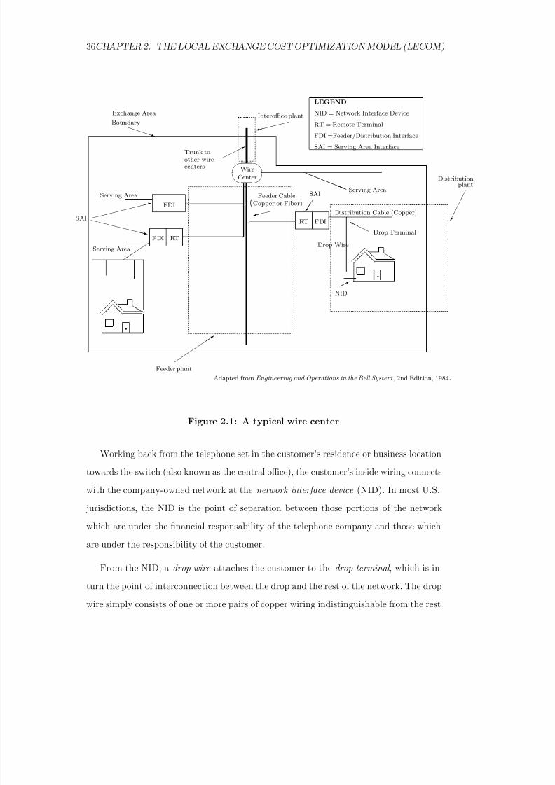
2.2 The Local Exchange Network: An Overview
The local exchange network is composed of four major components: distribution, feeder,
switching, and interoffice plant. Figure 2.1 below shows a stylized network incorporating
the major components and subcomponents.
8/18/2019 Gasmi Cost Proxy Models
http://slidepdf.com/reader/full/gasmi-cost-proxy-models 36/318
36CHAPTER 2. THE LOCAL EXCHANGE COST OPTIMIZATION MODEL (LECOM)
FDI RT
FDI
Wire
Center
Serving Area
Serving Area
RT FDI
Feeder Cable(Copper or Fiber)
SAI
Serving Area
NID
Drop Wire
Distribution Cable (Copper)
Drop Terminal
SAI
Trunk toother wirecenters
Exchange AreaBoundary
Interoffice plant
Feeder plant
LEGEND
NID = Network Interface DeviceRT = Remote Terminal
FDI =Feeder/Distribution Interface
SAI = Serving Area Interface
Adapted from Engineering and Operations in the Bell System , 2nd Edition, 1984.
Distributionplant
Figure 2.1: A typical wire center
Working back from the telephone set in the customer’s residence or business location
towards the switch (also known as the central office), the customer’s inside wiring connects
with the company-owned network at the network interface device (NID). In most U.S.
jurisdictions, the NID is the point of separation between those portions of the network
which are under the financial responsability of the telephone company and those which
are under the responsibility of the customer.
From the NID, a drop wire attaches the customer to the drop terminal , which is in
turn the point of interconnection between the drop and the rest of the network. The drop
wire simply consists of one or more pairs of copper wiring indistinguishable from the rest

8/18/2019 Gasmi Cost Proxy Models
http://slidepdf.com/reader/full/gasmi-cost-proxy-models 37/318
2.2. THE LOCAL EXCHANGE NETWORK: AN OVERVIEW 37
of the copper wiring that makes up the telephone network (except perhaps by its gauge).
The drop terminal is nothing more than a metal or plastic box in which the drop wireis spliced to the distribution backbone . Distribution backbone cables typically follow the
street or road grid pattern of a local geographical area, called a distribution area or serving
area , ultimately attaching to a serving area interface (SAI). The components described
up to the SAI collectively constitute what is known as the distribution plant .5
The SAI may take one of several forms, depending on engineering considerations. For
serving areas close to the central office, particularly areas with a residential customerbase, the SAI is likely to be a simple feeder-distribution interface (FDI). Like the drop
terminal but built to a larger scale, the FDI is nothing more than a box in which copper
cables are spliced together.
Other serving areas may require the use of a remote terminal (RT) designed to work
with digital technology, either some form of T1 (digital signal sent on copper plant) or
fiber optics. In these cases, some electronic equipment is necessary to convert to multiplex
(multi-channel) digital signals. In the case of a fiber optic RT, additional electronics are
used for conversion between optical signals and electronic impulses.
The fiber or copper (digital or analog) plant that carries telecommunications traffic
between the SAI and the switch is known as the feeder plant . At the switch, incoming
traffic is connected to the appropriate destination channel. If that channel is directly
connected to the switch, such traffic is termed intraoffice traffic . Otherwise, it is con-
sidered as interoffice traffic and directed to the appropriate switch via interoffice trunks .
Several functions besides basic switching may be performed at the switch level. First, any
analog interoffice traffic must be converted to digital, since virtually all interoffice trunks
are digital. Second, any advanced services (such as call-waiting, three-party calling, etc.)
are accommodated with additional hardware and software features. Finally, signaling (for
example, the ringing of a particular telephone) may be directed to a separate signaling
network.
8/18/2019 Gasmi Cost Proxy Models
http://slidepdf.com/reader/full/gasmi-cost-proxy-models 38/318
38CHAPTER 2. THE LOCAL EXCHANGE COST OPTIMIZATION MODEL (LECOM)
2.3 Technological Foundations of LECOM
In this section, we describe in detail the assumptions made on each type of plant modeled
in LECOM. Recall from the previous section that the local exchange network is essentially
viewed as the combination of, and interaction among, four elements: distribution, feeder,
switching and interoffice plant. The main design and technological aspects of these four
components are examined in turn.
2.3.1 The Distribution Plant
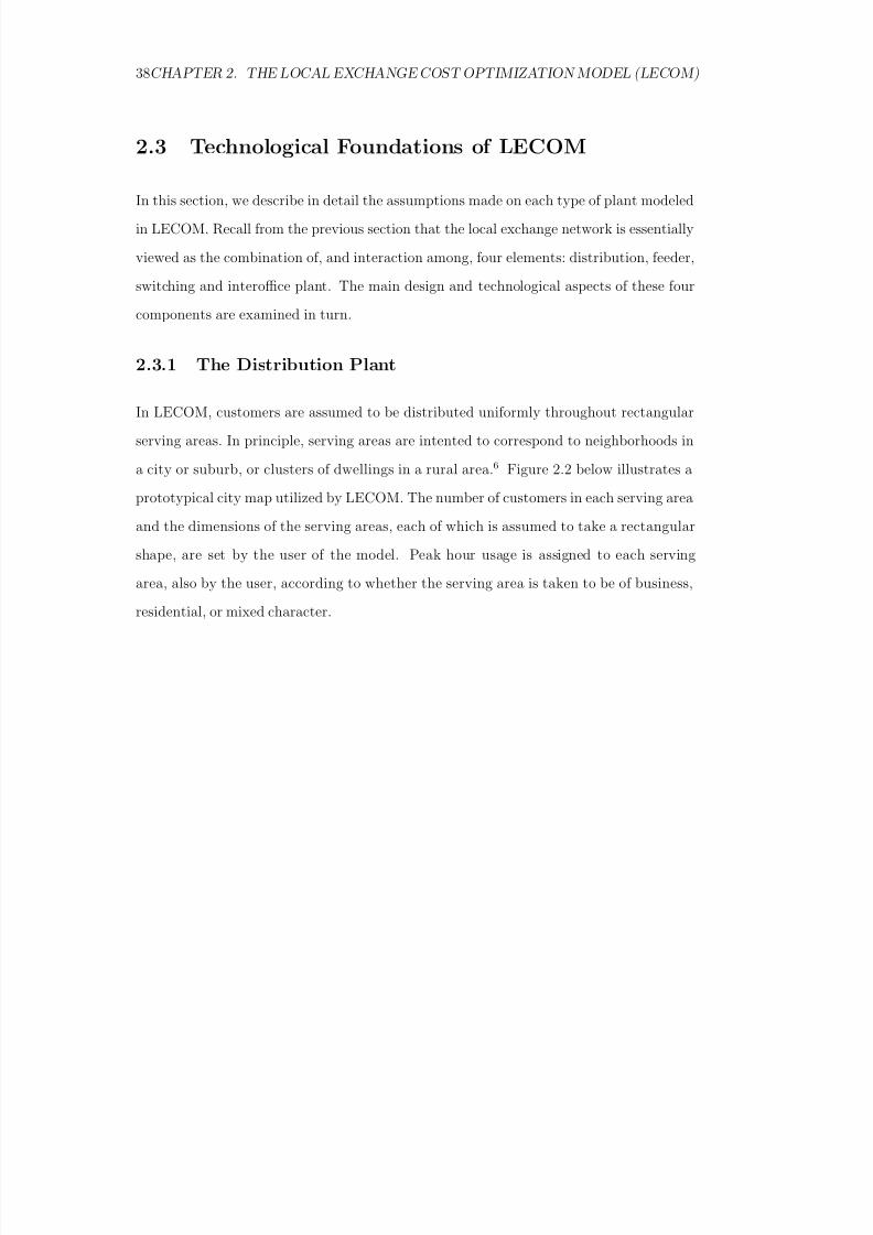
In LECOM, customers are assumed to be distributed uniformly throughout rectangular
serving areas. In principle, serving areas are intented to correspond to neighborhoods in
a city or suburb, or clusters of dwellings in a rural area. 6 Figure 2.2 below illustrates a
prototypical city map utilized by LECOM. The number of customers in each serving area
and the dimensions of the serving areas, each of which is assumed to take a rectangular
shape, are set by the user of the model. Peak hour usage is assigned to each serving
area, also by the user, according to whether the serving area is taken to be of business,
residential, or mixed character.
8/18/2019 Gasmi Cost Proxy Models
http://slidepdf.com/reader/full/gasmi-cost-proxy-models 39/318
2.3. TECHNOLOGICAL FOUNDATIONS OF LECOM 39
Central Business DistrictServing Area
Medium Density RegionServing Area
Suburban RegionServing Area
Figure 2.2: A stylized city map
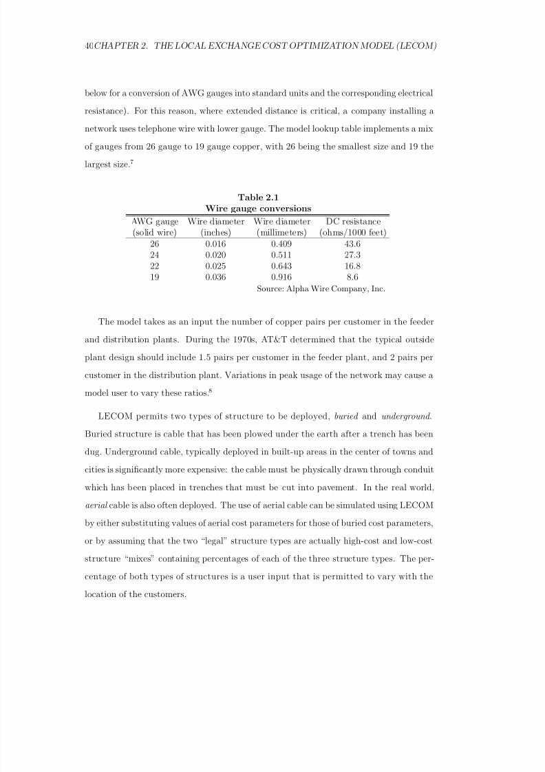
The distribution plant is assumed to carry analog signals over copper pairs. The gauge
of copper wire used is determined by how far the maximum-distance customer is from theswitch using a lookup table that is based on engineering principles. AWG (American Wire
Gauge) is a U.S. standard set of non-ferrous wire conductor sizes. The “gauge” means
the diameter. Non-ferrous includes copper and also aluminum and other materials, but is
most frequently applied to copper household electrical wiring and telephone wiring. In the
U.S., typical household electrical wiring is AWG number 12 or 14, while telephone wire is
usually 22, 24, or 26. Higher gauge numbers correspond to smaller diameters and thinner
(and less costly) wires. Since thicker wire carries more current because it has less electrical
resistance over a given length, thicker wire is better for longer distances (see Table 2.1
8/18/2019 Gasmi Cost Proxy Models
http://slidepdf.com/reader/full/gasmi-cost-proxy-models 40/318
40CHAPTER 2. THE LOCAL EXCHANGE COST OPTIMIZATION MODEL (LECOM)
below for a conversion of AWG gauges into standard units and the corresponding electrical
resistance). For this reason, where extended distance is critical, a company installing anetwork uses telephone wire with lower gauge. The model lookup table implements a mix
of gauges from 26 gauge to 19 gauge copper, with 26 being the smallest size and 19 the
largest size.7
Table 2.1Wire gauge conversions
AWG gauge Wire diameter Wire diameter DC resistance(solid wire) (inches) (millimeters) (ohms/1000 feet)
26 0.016 0.409 43.624 0.020 0.511 27.322 0.025 0.643 16.819 0.036 0.916 8.6
Source: Alpha Wire Company, Inc.
The model takes as an input the number of copper pairs per customer in the feeder
and distribution plants. During the 1970s, AT&T determined that the typical outside
plant design should include 1.5 pairs per customer in the feeder plant, and 2 pairs per
customer in the distribution plant. Variations in peak usage of the network may cause a
model user to vary these ratios.8
LECOM permits two types of structure to be deployed, buried and underground .
Buried structure is cable that has been plowed under the earth after a trench has been
dug. Underground cable, typically deployed in built-up areas in the center of towns andcities is significantly more expensive: the cable must be physically drawn through conduit
which has been placed in trenches that must be cut into pavement. In the real world,
aerial cable is also often deployed. The use of aerial cable can be simulated using LECOM
by either substituting values of aerial cost parameters for those of buried cost parameters,
or by assuming that the two “legal” structure types are actually high-cost and low-cost
structure “mixes” containing percentages of each of the three structure types. The per-
centage of both types of structures is a user input that is permitted to vary with the
location of the customers.
8/18/2019 Gasmi Cost Proxy Models
http://slidepdf.com/reader/full/gasmi-cost-proxy-models 41/318
2.3. TECHNOLOGICAL FOUNDATIONS OF LECOM 41
Since in LECOM customers are assumed to be uniformly distributed throughout each
neighborhood serving area, a simplified route structure is used. The distribution routingincludes a backbone running the length of the rectangle. At intervals equal to the (user
input) width of a city block, distribution branch cables run from the backbone to each
border and drops are added uniformly along the branch cable. Both branch cables and
distribution backbones “telescope”, that is, at each point of the distribution network,
the size of cable used reflects only the number of pairs needed at the given point and no
more.9 All distances in the distribution module are calculated in a rectilinear fashion with
axes running north-south and east-west. Figure 2.3 illustrates a prototypical distribution
serving area in LECOM.
Serving Area Interface
Distribution backbone
Distribution branch cable
Customer drops
Figure 2.3: A distribution serving area

8/18/2019 Gasmi Cost Proxy Models
http://slidepdf.com/reader/full/gasmi-cost-proxy-models 42/318
42CHAPTER 2. THE LOCAL EXCHANGE COST OPTIMIZATION MODEL (LECOM)
2.3.2 The Feeder Plant
Feeder plant runs from the serving area interface (SAI) to the central office.10 In LECOM,
feeder technology is chosen from three available technologies: analog on copper, digital
(T1) on copper, and digital on fiber.11 The model calculates the economic crossover points,
i.e., the route distance from the switch at which one technology is substituted for another,
for these three technologies based on cost. The user can override the model’s choice by
specifying alternative crossover points based on other criteria such as quality-of-service.12
If a digital feeder technology is chosen, the model “installs” a SLC-96 concentrator at the
serving area interface.13
Gauge for feeder pairs carried on analog copper pairs are chosen from the same gauge-
distance table used in the distribution plant. It is always assumed that T1 pairs are of
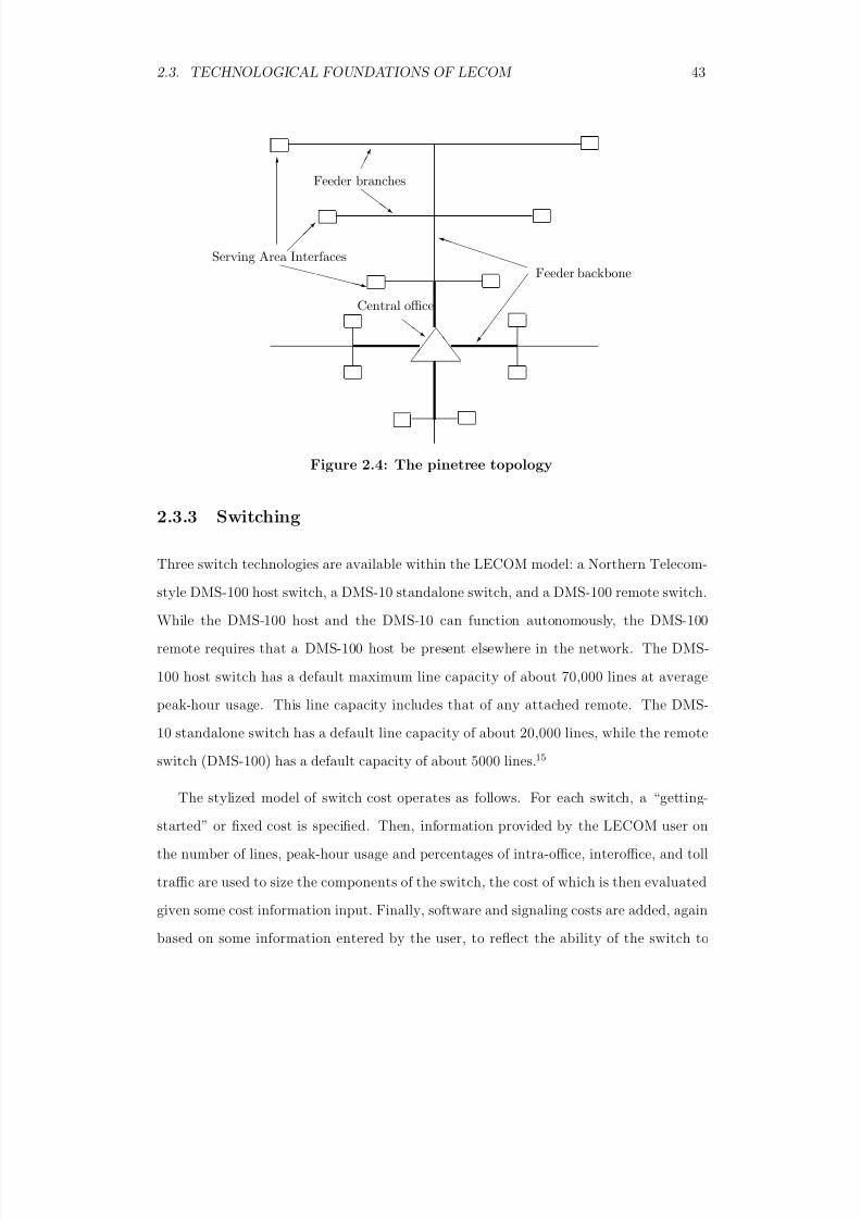
24-gauge copper. As to feeder routing, it is implemented using the relatively standard “
pinetree” design. The pinetree design consists of a main backbone shared by all serving
areas and each serving area connected to the backbone by means of a unique branch. 14
As in the distribution case, feeder distances are rectilinear with axes running north-
south and east-west, and feeder cables of all types are telescoped, with analog copper,
digital copper, and fiber optic cables handled separately (i.e., not carried in the same
cables). Figure 2.4 illustrates the feeder plant design used in LECOM.
8/18/2019 Gasmi Cost Proxy Models
http://slidepdf.com/reader/full/gasmi-cost-proxy-models 43/318
2.3. TECHNOLOGICAL FOUNDATIONS OF LECOM 43
Serving Area Interfaces
Feeder branches
Feeder backbone
Central office
Figure 2.4: The pinetree topology
2.3.3 Switching
Three switch technologies are available within the LECOM model: a Northern Telecom-
style DMS-100 host switch, a DMS-10 standalone switch, and a DMS-100 remote switch.
While the DMS-100 host and the DMS-10 can function autonomously, the DMS-100
remote requires that a DMS-100 host be present elsewhere in the network. The DMS-
100 host switch has a default maximum line capacity of about 70,000 lines at average
peak-hour usage. This line capacity includes that of any attached remote. The DMS-
10 standalone switch has a default line capacity of about 20,000 lines, while the remote
switch (DMS-100) has a default capacity of about 5000 lines. 15
The stylized model of switch cost operates as follows. For each switch, a “getting-
started” or fixed cost is specified. Then, information provided by the LECOM user on
the number of lines, peak-hour usage and percentages of intra-office, interoffice, and toll
traffic are used to size the components of the switch, the cost of which is then evaluated
given some cost information input. Finally, software and signaling costs are added, again
based on some information entered by the user, to reflect the ability of the switch to
8/18/2019 Gasmi Cost Proxy Models
http://slidepdf.com/reader/full/gasmi-cost-proxy-models 44/318
44CHAPTER 2. THE LOCAL EXCHANGE COST OPTIMIZATION MODEL (LECOM)
handle the so-called advanced services.
Each switch’s capacity interacts critically with customer location data. First, serving
areas are sorted according to their population and a provisional cost of attachment to each
switch is calculated for each serving area. Beginning with the most populated serving area,
each serving area is attached to the least costly switch that has remaining capacity. That
is, let P C (i, j) be the provisional cost of attaching the serving area indexed by i to the
switch indexed by j. Let K j be the capacity (in terms of the number of lines) of switch
j and T j the number of lines already served by this switch. Then, serving area k willeffectively be attached to switch l if
l = arg min j
P C (k, j) and K l − T l − N k ≥ 0 (2.1)
where N k is the serving area k’s population.
Because of the capacity constraints imposed on each individual switch (LECOM does
not permit collocation of switches), it is possible however that the configuration of switches
so found be not globally optimal. In order to alleviate this shortcoming, the model permits
switches to “trade” serving areas according to the following rule. Assume that serving
areas i and j are attached to switches k and l, respectively. Then, these switches may
trade the serving areas, i.e., serving area i becomes attached to switch l and serving area
j to switch k if
T k − N i + N j ≤ K k and T l − N j + N i ≤ K l and P C ( j, k) + P C (i, l) < P C (i, k) + P C ( j, l)
(2.2)
where the T ’s, N ’s, K ’s and P C ’s are as defined above.
Finally, as far as remote switches are concerned each of these switches is assigned to
the most proximate host switch up to the maximum number of remote switches attachable
to a host or standalone switch which is by default equal to 6.16 Remote switches serve
8/18/2019 Gasmi Cost Proxy Models
http://slidepdf.com/reader/full/gasmi-cost-proxy-models 45/318
2.3. TECHNOLOGICAL FOUNDATIONS OF LECOM 45
to transfer most of the switching functionality of the host switch to a remote location,
thereby reducing the load on the host switch and enabling the remote traffic to benefitfrom the economies associated with sharing transport plant from the remote location to
the host location. Intraoffice capability is maintained at the remote location, but all
interoffice traffic must go through the host switch.
2.3.4 The Interoffice Plant
The cost of interoffice plant in LECOM is treated by calculating the number of trunksrequired between each pair of central offices present in the area being considered. A
critical parameter used in this calculation is, for each switch, the interoffice portion of
peak-hour traffic per line (set by the LECOM user) multiplied by the number of lines
served by the switch. This aggregate traffic handled by a given switch is distributed to
the other switches of the network according to a formula that takes into account the
distance from those switches to the original switch (the closer a switch the more traffic it
gets). The traffic so calculated is then applied to a table based on engineering principles
that gives the number of interoffice trunks required to handle originating traffic from the
given switch.17 The fraction of total interoffice traffic originating from switch k which is
allocated to switch j, rkj , is given by
rkj = j2i=k
i2(2.3)
where the switches i = k are sorted by descending order of distance from switch k.18
Figure 2.5 below illustrates the interoffice design used by LECOM. In this figure, the
trunk to each switch’s most proximate neighbor is indicated by a relatively thick link,
trunks between second most proximate neighbors are denoted by a link of intermediate
thickness and the most distant neighbors are linked by the thinnest links. The figure also
illustrates a host-remote link, showing how remote switches only directly communicate
with the host switch to which they are attached.
In addition to links between local switches located in the map region, LECOM also
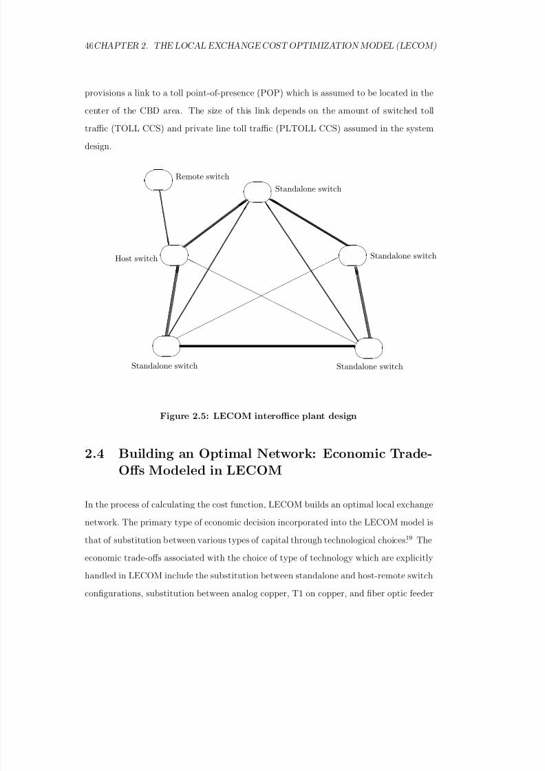
8/18/2019 Gasmi Cost Proxy Models
http://slidepdf.com/reader/full/gasmi-cost-proxy-models 46/318
46CHAPTER 2. THE LOCAL EXCHANGE COST OPTIMIZATION MODEL (LECOM)
provisions a link to a toll point-of-presence (POP) which is assumed to be located in the
center of the CBD area. The size of this link depends on the amount of switched tolltraffic (TOLL CCS) and private line toll traffic (PLTOLL CCS) assumed in the system
design.
Remote switch
Standalone switch
Host switch
Standalone switch Standalone switch
Standalone switch
Figure 2.5: LECOM interoffice plant design
2.4 Building an Optimal Network: Economic Trade-Offs Modeled in LECOM
In the process of calculating the cost function, LECOM builds an optimal local exchange
network. The primary type of economic decision incorporated into the LECOM model is
that of substitution between various types of capital through technological choices.19 The
economic trade-offs associated with the choice of type of technology which are explicitly
handled in LECOM include the substitution between standalone and host-remote switch
configurations, substitution between analog copper, T1 on copper, and fiber optic feeder

8/18/2019 Gasmi Cost Proxy Models
http://slidepdf.com/reader/full/gasmi-cost-proxy-models 47/318
2.4. BUILDING AN OPTIMAL NETWORK: ECONOMIC TRADE-OFFS MODELED...47
technologies, and the trade-off between added electronics in the form of more switches
and building of loop plant in the form of longer loop lengths. Furthermore, in its mosttechnologically advanced feature, LECOM takes into account trade-offs in the locations
of switches between centralization of local demand and the cost of interconnection.
In effect the third trade-off described above can be thought of as a generalization of
the first since remote switches are really just extra switches being added for the purpose
of reducing loop lengths and, as in the more conventional interpretation, of redistributing
traffic loads to more decentralized locations. However, a distinction is made betweenthese trade-offs in that, in the model, the host-remote system exists solely to exploit any
economies of concentrated loop plant, while the trade-off between host-remote systems
and standalones also captures the traffic redistribution effect. This is because remote
interoffice plant is assumed to connect only to hosts, while standalone switches connect
directly via trunks with all other switches in the network.
If quality of service is held constant at a voice-grade level, for any location within
a certain distance from the central office, which is determined by line resistance and
impedance, service is provided most economically, given current levels of cost of material,
through analog copper pairs passing through the feeder and distribution plants directly to
the customer location from the switch. As this distance increases, voice grade service on
analog plant requires load coils, a type of amplifier, to improve signal quality, as well as
an increase in the gauge (thickness) of copper used. As an alternative, digital signals may
be transmitted over specially conditioned copper (T1) or fiber optic plant, but the signals
must be converted electronically at a remote location for use as voice communication
which requires a significant investment in electronic equipment at the site. The model
explicitly models this trade-off by creating a set of economic crossover points that is uses
to replace analog copper with digital copper, and digital copper with digital fiber.
The choice of any switch’s location is sensitive to two conflicting factors: the distance
of that switch from its served customers and its distance from its points of interconnection
with the rest of the network. While the latter costs are relatively small, typically of the
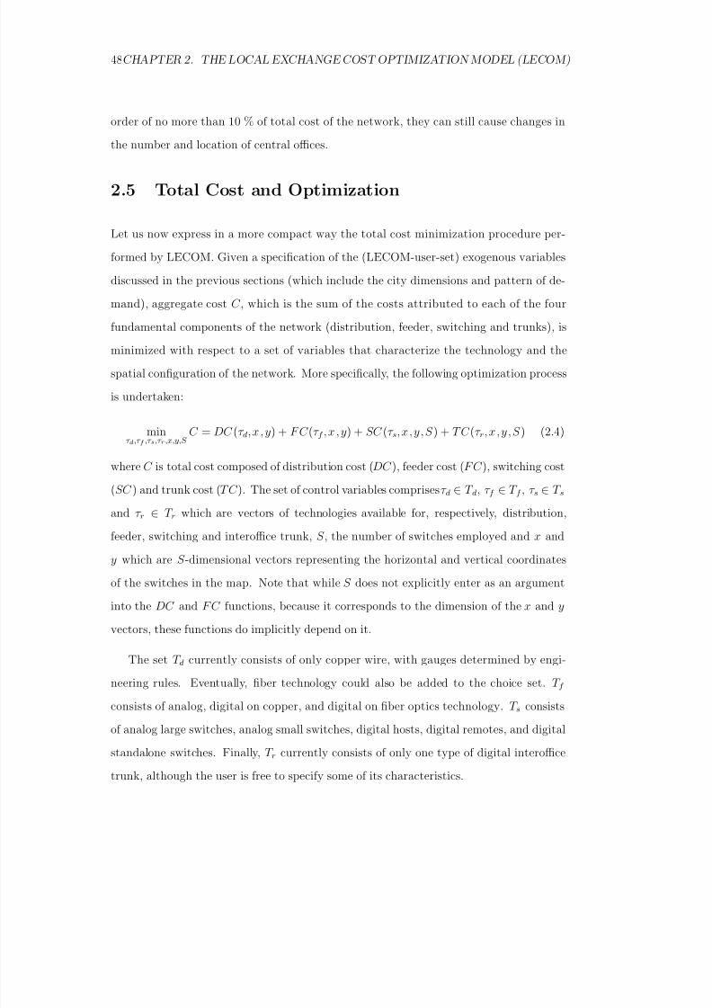
8/18/2019 Gasmi Cost Proxy Models
http://slidepdf.com/reader/full/gasmi-cost-proxy-models 48/318
48CHAPTER 2. THE LOCAL EXCHANGE COST OPTIMIZATION MODEL (LECOM)
order of no more than 10 % of total cost of the network, they can still cause changes in
the number and location of central offices.
2.5 Total Cost and Optimization
Let us now express in a more compact way the total cost minimization procedure per-
formed by LECOM. Given a specification of the (LECOM-user-set) exogenous variables
discussed in the previous sections (which include the city dimensions and pattern of de-
mand), aggregate cost C , which is the sum of the costs attributed to each of the four
fundamental components of the network (distribution, feeder, switching and trunks), is
minimized with respect to a set of variables that characterize the technology and the
spatial configuration of the network. More specifically, the following optimization process
is undertaken:
minτ d,τ f ,τ s,τ r,x,y,S
C = DC (τ d, x , y) + F C (τ f , x , y) + SC (τ s, x , y, S ) + T C (τ r, x , y, S ) (2.4)
where C is total cost composed of distribution cost (DC ), feeder cost (F C ), switching cost
(SC ) and trunk cost (T C ). The set of control variables comprises τ d ∈ T d, τ f ∈ T f , τ s ∈ T s
and τ r ∈ T r which are vectors of technologies available for, respectively, distribution,
feeder, switching and interoffice trunk, S , the number of switches employed and x and
y which are S -dimensional vectors representing the horizontal and vertical coordinates
of the switches in the map. Note that while S does not explicitly enter as an argument
into the DC and F C functions, because it corresponds to the dimension of the x and y
vectors, these functions do implicitly depend on it.
The set T d currently consists of only copper wire, with gauges determined by engi-
neering rules. Eventually, fiber technology could also be added to the choice set. T f
consists of analog, digital on copper, and digital on fiber optics technology. T s consists
of analog large switches, analog small switches, digital hosts, digital remotes, and digital
standalone switches. Finally, T r currently consists of only one type of digital interoffice
trunk, although the user is free to specify some of its characteristics.

8/18/2019 Gasmi Cost Proxy Models
http://slidepdf.com/reader/full/gasmi-cost-proxy-models 49/318
2.5. TOTAL COST AND OPTIMIZATION 49
The search for optimal switch location is accomplished by the derivative-free search
algorithm proposed by Nelder and Mead (1965), as described in Press et al. (1986), overthe x and y - coordinates of a map representing in a discrete fashion the city being served
by the telephone network.20 This derivative-free algorithm suits particularly well our
problem for two reasons. First, LECOM assumes that all cabling in the city follows city
streets, which are set in a rectangular grid patter, so that the L1 norm (sum of absolute
deviations) is the relevant distance measure. Second, since copper wire is only available in
a finite number of gauges, the relationship between distance from wire center to customer
and cabling cost is not smooth.21
Figure 2.6 below illustrates the nested optimization process. The model takes as data
the dimensions of a city, customer distribution and usage levels. LECOM then searches
for the technological mix, capacity, number and location of switches that minimize the
annual cost of production. This is equivalent to minimizing the present value of capital
cost and operation, maintenance and tax expenditures. Each of capital cost, depreciation
expense, operating expense, maintenance expense, and taxes is expressed as a percentage
of investment in each network component, and these percentages are summed up to form
the annual charge factor . For example, if the cost of capital is 7%, depreciation is 10%
and the cost of operation and maintenance is 6%, the annual charge factor would be
0.23 (23%). Annual charge factors are one mechanism through which labor costs are
introduced into the model. Indeed, operating and maintenance expenses are largely labor
costs (as well as some material cost). Labor costs are also incorporated in the cost of
installation, which is assumed to be part of the first cost, or initial investment, in each
piece of equipment. The optimal locations of the switches are found by means of the
nonlinear derivative-free routine mentioned earlier.
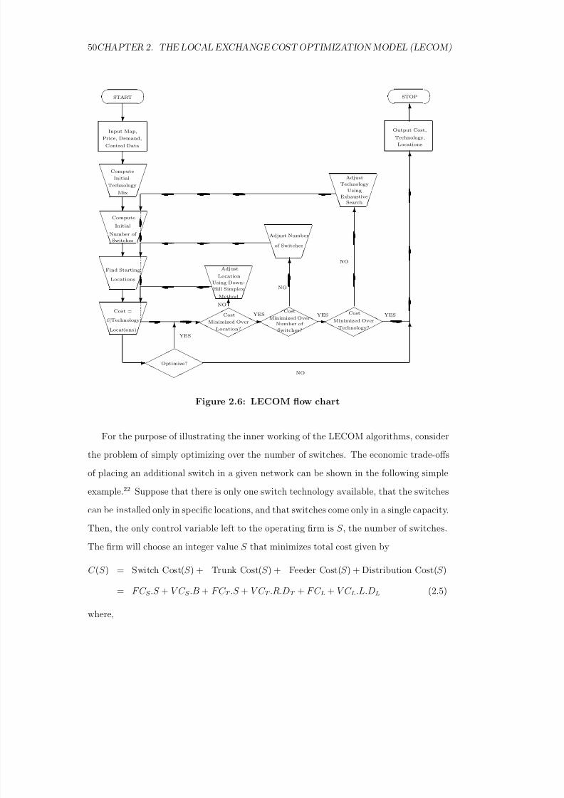
8/18/2019 Gasmi Cost Proxy Models
http://slidepdf.com/reader/full/gasmi-cost-proxy-models 50/318
50CHAPTER 2. THE LOCAL EXCHANGE COST OPTIMIZATION MODEL (LECOM)
START
Input Map,
Price, Demand,
Control Data
Compute
Initial
Technology
Mix
Compute
Initial
Number of Switches
Find Starting
Locations
Cost =
f(Technology,
Locations)
Optimize?
YES
Cost
Minimized Over
Location?
NO
YES YES
NO
NO
Adjust
Location
Using Down-
Hill Simplex
Method
Adjust Number
of Switches
Adjust
Technology
Using
ExhaustiveSearch
Cost
Minimized OverNumber of
Switches?
Cost
Minimized Over
Technology?
YES
Output Cost,
Technology,
Locations
STOP
NO
Figure 2.6: LECOM flow chart
For the purpose of illustrating the inner working of the LECOM algorithms, consider
the problem of simply optimizing over the number of switches. The economic trade-offs
of placing an additional switch in a given network can be shown in the following simple
example.22 Suppose that there is only one switch technology available, that the switches
can be installed only in specific locations, and that switches come only in a single capacity.
Then, the only control variable left to the operating firm is S , the number of switches.
The firm will choose an integer value S that minimizes total cost given by
C (S ) = Switch Cost(S ) + Trunk Cost(S ) + Feeder Cost(S ) + Distribution Cost(S )
= F C S .S + V C S .B + F C T .S + V C T .R.DT + F C L + V C L.L.DL (2.5)
where,

8/18/2019 Gasmi Cost Proxy Models
http://slidepdf.com/reader/full/gasmi-cost-proxy-models 51/318
2.5. TOTAL COST AND OPTIMIZATION 51
C (S ) is the total cost expressed only as a function of S , the number of switches
DT is the average distance per trunk (depends on S )
DL is the average loop length (depends on S )
R is the number of interoffice trunks (depends on S )
F C L is the fixed cost of loops for a given city size (exogenous cost parameter)
F C S is the fixed cost of a switch (exogenous cost parameter)
F C T is the fixed cost of terminating a trunk of any size at a switch (exogenous cost
parameter)
V C L is the variable cost per unit of distance of loop plant (exogenous cost parameter)
V C S is the variable switching cost per hundred busy-hour calling seconds (exogenous cost
parameter)
V C T is the variable cost per unit of distance of trunk plant (exogenous cost parameter)
L is the number of loops (exogenous demand parameter)
B represents hundreds of busy-hour calling seconds (exogenous demand parameter)
In general, one would expect
∂R
∂S > 0,
∂DL
∂S < 0, and
∂DT
∂S < 0 (2.6)
that is, as the number of switches increases, the number of trunks increases while theaverage loop length and the average trunk length decrease.23 If equation (2.5) were
differentiable, the first-order condition of this optimization problem would be24
∂C
∂S = F C S + F C T + V C T
DT
∂R
∂S + R
∂DT
∂S
+ V C LL
∂DL
∂S ∼= 0. (2.7)
In fact, since only integer values of S (the number of switches) are acceptable, we
cannot set this equation exactly equal to zero. Hence, if the derivative ∂C/∂S is neg-
ative, i.e., total cost declines when an additional switch is deployed, then the switch

8/18/2019 Gasmi Cost Proxy Models
http://slidepdf.com/reader/full/gasmi-cost-proxy-models 52/318
52CHAPTER 2. THE LOCAL EXCHANGE COST OPTIMIZATION MODEL (LECOM)
is added. The motivation is that a switch should be added if the additional fixed
cost of switching and trunks (F C S + F C T ) to which we add the cost of the additionaltrunks V C T DT (∂R/∂S ) is less than the cost savings from shorter loops and trunks
V C T R(∂DT /∂S ) + V C LL(∂DL/∂S ).25
Table 2.2 below gives the pseudo-code for the LECOM cost function. In the pseudo-
code, we see that equation (2.4) is integrated into the nested optimizations by declaring
cost as a function of technology, number of switches, and location. Table 2.2 also gives
an indication of how the switching, feeder, distribution, and trunk cost modules areintegrated.
It is worthwhile to make some comments on how these modules operate. For example,
the feeder module involves constructing the pinetree route design for feeder cables, which
in turn involves sorting the serving areas along each feeder main by distance. The module
(like the other modules computing cabling costs) exploits the economies associated with
bundling cables together, which enriches the optimization procedure. Furthermore, feeder
(as well as distribution and trunk) cables are assumed to follow only street grids, which
means that all distances are L1 (absolute deviation) norms rather than the more familiar
Cartesian norm.
The derivative-free algorithm for the location optimization, mentioned above, is par-
ticularly useful to handle the non linearity of some of the engineering functions that are
incorporated into the switching cost modules. Manufacturers of switches have developed
engineering algorithms that determine the appropriate physical quantities of equipment
for various levels of demand. For example, the number of multiplex loops in the DMS-
10 module, the number of line group controllers in DMS-100 and the number of remote
switches attached to the DMS-100 are all nonlinear functions of peak-period usage. 26
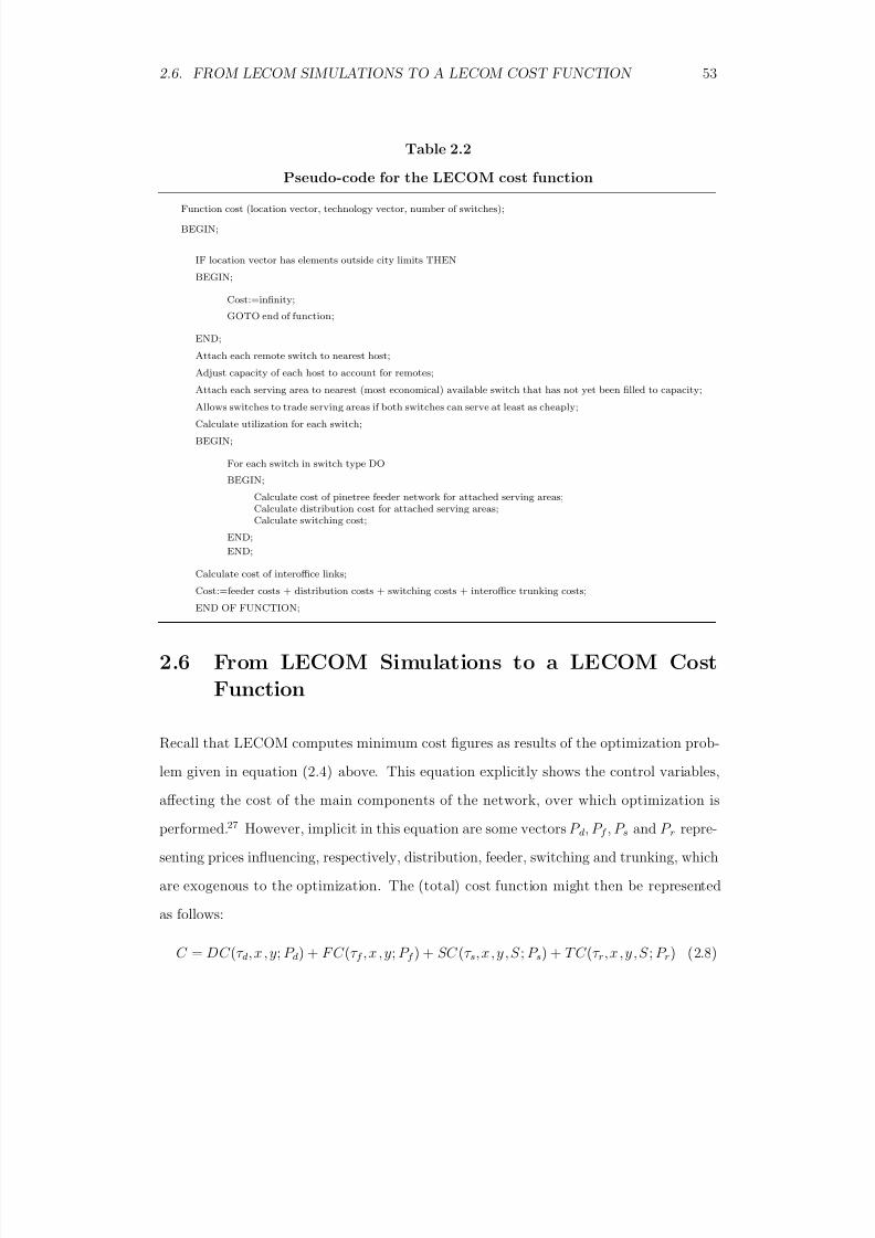
8/18/2019 Gasmi Cost Proxy Models
http://slidepdf.com/reader/full/gasmi-cost-proxy-models 53/318
2.6. FROM LECOM SIMULATIONS TO A LECOM COST FUNCTION 53
Table 2.2
Pseudo-code for the LECOM cost functionFunction cost (location vector, technology vector, number of switches);
BEGIN;
IF location vector has elements outside city limits THEN
BEGIN;
Cost:=infinity;
GOTO end of function;
END;
Attach each remote switch to nearest host;
Adjust capacity of each host to account for remotes;
Attach each serving area to nearest (most economical) available switch that has not yet been filled to capacity;
Allows switches to trade serving areas if both switches can serve at least as cheaply;
Calculate utilization for each switch;
BEGIN;
For each switch in switch type DO
BEGIN;
Calculate cost of pinetree feeder network for attached serving areas;Calculate distribution cost for attached serving areas;Calculate switching cost;
END;
END;
Calculate cost of interoffice links;
Cost:=feeder costs + distribution costs + switching costs + interoffice trunking costs;
END OF FUNCTION;
2.6 From LECOM Simulations to a LECOM CostFunction
Recall that LECOM computes minimum cost figures as results of the optimization prob-
lem given in equation (2.4) above. This equation explicitly shows the control variables,
affecting the cost of the main components of the network, over which optimization is
performed.27 However, implicit in this equation are some vectors P d, P f , P s and P r repre-
senting prices influencing, respectively, distribution, feeder, switching and trunking, which
are exogenous to the optimization. The (total) cost function might then be represented
as follows:
C = DC (τ d, x , y; P d) + F C (τ f , x , y; P f ) + SC (τ s, x , y, S ; P s) + T C (τ r, x , y, S ; P r) (2.8)

8/18/2019 Gasmi Cost Proxy Models
http://slidepdf.com/reader/full/gasmi-cost-proxy-models 54/318
54CHAPTER 2. THE LOCAL EXCHANGE COST OPTIMIZATION MODEL (LECOM)
Table 2.3 below lists some representative values for the user adjustable pricing inputs that
influence the cost of each of the four components of the network.28
Table 2.3Representative user adjustable LECOM inputs
Factor Price Multipliers0.676 labor factor price multiplier1.467 capital factor price multiplier1.000 central office material price multiplier1.000 outside plant material price multiplier
Annual Charge Factors0.313 carrying charge for land0.326 carrying charge for buildings0.301 carrying charge for circuit0.375 carrying charge for analog switches0.280 carrying charge for conduit0.281 carrying charge for underground cable0.316 carrying charge for buried cable0.316 carrying charge for underground fiber0.343 carrying charge for buried fiber
Prices for Outside Plant andSwitching Equipment1.682 fixed investment/foot of underground copper2.172 fixed investment/foot of buried copper0.007 marginal investment/foot of underground copper0.009 marginal investment/foot of buried copper1.575 fixed cost of underground fiber0.187 cost per foot of underground fiber2.778 fixed cost of buried fiber0.197 cost per foot of buried fiber30.00 cost per foot of conduit0.070 investment loading for building (circuit)0.070 investment loading for building (switch)0.005 investment loading for land (circuit)0.005 investment loading for land (switch)53.00 main distribution frame cost/customer21.37 1990 tandem investment per CCS∗
* Telecommunications traffic is measured in hundreds of busy-hour calling seconds, i.e., in CCS
where the first C is the Roman numeral for 100. This represents the time the average line is
used per hour during the peak period.

8/18/2019 Gasmi Cost Proxy Models
http://slidepdf.com/reader/full/gasmi-cost-proxy-models 55/318
2.6. FROM LECOM SIMULATIONS TO A LECOM COST FUNCTION 55
We separate the price inputs to LECOM into three categories. At the lowest level there
are factor prices for a broad range of materials and labor inputs for the telecommunicationsproduction function. These include the fixed and variable costs of deploying copper and
fiber cable and structures, as well as the costs of associated circuit equipment (electronics
required for digital/analog conversions) and switching equipment. Given these factor
prices, and a set of additional inputs which describe user demands and the characteristics
of the serving area, the LECOM optimization algorithms provide an estimate of the total
network investment required to provide local exchange service.
At the next level, there are additional input variables which describe the way in which
total network investment is converted to an annual (or monthly) cost per subscriber.
These annual charge factors include three distinct components:
1. the cost of capital, which represents the weighted average cost of debt and equity
financing for a representative firm in the industry,
2. the depreciation factor, which represents both the salvage value and the expected
economic life for each category of telecommunications plant and equipment, and
3. annual operating expenses for the firm, including maintenance, network planning
and corporate overhead expenses.
At the highest level, LECOM includes input values for factor price multipliers for
labor, capital, central office equipment and outside plant. These multipliers are intended
primarily to account for regional variations in the larger set of inputs that enter the
firm’s cost function. For example, a change in the value of the price multiplier for capital
will have a significant impact on the cost of cable, circuit equipment and switches, while
a change in the labor multiplier will have the greatest impact on the cost of structure
placements, maintenance activities and other labor intensive activities of the firm.
As is readily apparent from the foregoing discussion, a proper engineering specification
of the cost of a local exchange network is significantly more complex than traditional

8/18/2019 Gasmi Cost Proxy Models
http://slidepdf.com/reader/full/gasmi-cost-proxy-models 56/318
56CHAPTER 2. THE LOCAL EXCHANGE COST OPTIMIZATION MODEL (LECOM)
econometric specifications. Standard economic theory shows that the programming dual
to the problem of profit maximization is that of cost minimization; these problems leadto equivalent solutions in terms of the optimal choices of capital (K ), labor (L), and
materials (M ) inputs and levels of outputs. It is easy to show that the minimization of
cost given the level of output Q and input prices leads to a function
C (P K , P L, P M , Q) (2.9)
where the partial derivative of this function with respect to factor prices, P K , P L, and P M ,
gives the firm’s conditional factor demand for the respective inputs.29 For the purpose of
the book, this cost function might be expanded into its component-cost functions of prices
that correspond to the four fundamental modules retained in the design of the LECOM
network, namely, distribution, feeder, switching and trunking.
While traditional econometric specifications assume that such a function is smooth
and continuous, thereby leading to “nice” statistical specification properties, it is worth
noting that a cost function need not be expressible in an analytical form. One can simply
write down a table of costs along with associated input prices and output levels.
By varying input prices and levels of output, a simulation “ experiment” using LECOM
can be performed leading to such a table. In a later chapter of this book, we will describe
the features and details of such experiments. For our purposes we simply point out that
such a table can readily be treated in a manner similar to empirical data generated in
the real world. That is, the table contains independent observations on total cost, factor
prices, and output levels. It is then a simple matter to apply a traditional econometric
specification to these data. One must do so advisedly though, since no stochastic com-
ponent in the usual sense is present.30 This exercice is however worthwhile in that it is
possible to summarize the properties of the cost function underlying the data (i.e., the
LECOM simulation) in ways that are familiar to economists.
A full analytical representation of the aggregate cost function modeled by LECOM is
not feasible as the program uses a large number of integer search algorithms and cumulates

8/18/2019 Gasmi Cost Proxy Models
http://slidepdf.com/reader/full/gasmi-cost-proxy-models 57/318
2.6. FROM LECOM SIMULATIONS TO A LECOM COST FUNCTION 57
costs by summing up the costs of individual network components which connect the
population of customers. Nevertheless, Equations (2.4), (2.5) and (2.8) express differentconceptual views of the same underlying cost function, which by the design of LECOM
as an optimizing process, are fully consistent with the representation of “... all of the
economically relevant aspects of the technology” (Varian, 1992) of the local exchange by
a cost function as required by economic theory.
An overly simplified representation of this cost function might be obtained by expand-
ing Equation (2.5) as follows:
C (P K , P L, P M ; L,S,CCS,R) = F C S (P K , P L, P M ; S,CCS ).S
+CCS.V CC S (P K , P L, P M ; S,CCS ) + F C T (P K , P L, P M ; R,CCS ).S
+V C T (P K , P L, P M ; R,CCS ).R.DT + F C L(P K , P L, P M ; L) + V C L(P K , P L, P M ; L).L.DL
(2.10)
A change in any of the underlying input parameters in equation (2.4) will lead to
a more or less complicated change in total cost. For example, a change in one of the
“demand” parameters will directly affect one or more of the quantities L,S,CCS and
R, which will in turn lead to a direct multiplicative effect as can be seen from (2.10).
In addition, there will be an indirect effect to the extent that the fixed and variable
cost functions depend on these quantities. Similarly, a change in any of the underlying
input prices P K , P L and P M will have a direct impact through the fixed and variable cost
functions as well as an indirect impact to the extent that such a change in prices results
in a substitution effect among the technologies which the LECOM algorithm chooses to
deploy. Any change in relative price can, in principle, result in a redesigned network which
will be reflected in the distance functions DL and DT as well as the number of switches
S that LECOM selects.
8/18/2019 Gasmi Cost Proxy Models
http://slidepdf.com/reader/full/gasmi-cost-proxy-models 58/318
58 NOTES
Notes
1This model was developed as part of a research grant from the National Regulatory
Research Institute (see Gabel and Kennet, 1991).
2A reader not familiar with the technology of voice telecommunications at the local
exchange level may wish to consult some outside sources in order to have a better under-
standing of the LECOM cost model. See, for example, Sharkey (2001).
3
Digital technology is now the dominant technology in telecommunications for bothswitching and transmission functions. When a subscriber is served by a digital switch,
voice signals must be converted from an analog to a digital format and this can be done
either at the central office or at the serving area interface level. If this conversion is done
in the field, concentrating the resulting digital signals on a reduced number of pairs of
copper or fiber optic cables leads to some cost savings. This concentration technology is
referred to as subscriber-line-carrier.
4While copper cables are available in the model in four different sizes (gauges), 26,24,22
and 19- gauge wire, fiber optic cable comes only in one size (see Section 3.1 for the more
precise meaning of these gauges). The installed size of copper wire critically depends on
the distance to be covered and the desired level of quality of communications. The shorter
the distance, the smaller the diameter of the copper cable that can be used and hence
the lower the cost. The drawback, however, is that smaller size cables have more electric
resistance than larger ones, which could impede communications. Gauge bears no direct
relation with the amount of traffic that a line can handle.
5LECOM assumes that distribution cables are always copper, the technology of choice
for voice-grade only networks. In other words, the model at this time does not handle
“fiber to the curb,” possibly the next generation of distribution technology.
6Typically, a serving area contains 350 to 600 subscribers.
7See footnote 3 above for the factors that determine the choice of gauge in the dis-

8/18/2019 Gasmi Cost Proxy Models
http://slidepdf.com/reader/full/gasmi-cost-proxy-models 59/318
NOTES 59
tribution plant. Those same considerations are taken into account when determining the
proper gauge of cable in the feeder plant (see Section 2.3.2 below). See also Section 2.4below.
8These standards have been established by AT&T in order to allow users to possess a
second line and provide spare capacity in the distribution and feeder plants in anticipating
of high level of usage (see Stiles, 1978).
9Note, however, that cable is available only in discrete sizes. Thus, suppose the total
pairs required by customers at point A (which is more distant from the switch) are 5, and
customers at point B have additional demand for 5 pairs. The smallest cable size used is
6 pairs, and the next larger size is 12 pairs. Thus, from point A to point B, a cable with
a capacity of 6 pairs is used, and from point B toward the SAI the cable size must be
increased to the next size 12 pairs. This is an example of “telescoping”.
10Recall, from Section 2.2, that the feeder network connects every area to a central
office and that the distribution plant provides a link for every customer in a given serving
area to a serving area interface (SAI).
11T1 is a U.S. standard in which 24 digital channels are carried over 2 copper pairs.
The European standard, E1, carries 30 digital channels over 2 pairs. In either case, the
deployment decision hinges on the relative cost of the copper (a function of the distance
the signal must travel), expected traffic (a “ concentrated” digital channel shares the
capacity of the copper line with other channels, while an analog line is dedicated), and
the cost of the electronics required to convert the digital signal to analog so that the
customer is able to use it.
12Long analog copper runs may impede the ability of the network to support high-speed
services.
13
SLC-96 (subscriber-line-carrier) is the subscriber-line concentrator that has typically
been used by the Bell Operating Companies (see footnote 2 above for a discussion of the

8/18/2019 Gasmi Cost Proxy Models
http://slidepdf.com/reader/full/gasmi-cost-proxy-models 60/318
60 NOTES
role of the subscriber-line-carrier technology).
14Recently, a minimum cost spanning tree type algorithm, which is more general than
the pinetree method, has been used to model feeder routing (see Bush et al., 1999). For
computational efficiency reasons, however, the pinetree algorithm might still be desirable
as it requires no iterative procedures, searching or sorting.
15Switching capacity can be changed by the LECOM user, although it is usually set
once and for all.
16This parameter may be increased up to 9 by the LECOM user.
17In general, the greater peak usage, the larger the ratio of interoffice trunk lines to
single-channel local loops (see, e.g., Engineering and Operations in the Bell System , 1983).
18Note that this interoffice trunk model builds interoffice trunks between every pair of
switches. Alternatively, SONET technology only requires that a switch belong to one or
more rings of interconnected switches and hence would most likely lead to less interoffice
plant overall.
19LECOM is less successful in explicitly modeling substitution between capital and la-
bor, although implicitly this too is possible. This is accomplished through the model’s
use of annual charge factors, which include a labor loading on each piece of capital equip-
ment used in the optimization. Thus, the cost of labor is taken into account when the
optimization is performed and trade-offs can be explored by varying the capital and labor
cost indexes which are input parameters in LECOM.
20To alleviate the problem of local optimum, LECOM restarts the optimization a certain
number of times specified by the user, by randomly adjusting the initial values.
21Recall that as distance traversed by copper wire increases, thicker wire is required in
order to compensate for electrical energy losses.
22For the purpose of the example, we simplify the exposition by merging distribution

8/18/2019 Gasmi Cost Proxy Models
http://slidepdf.com/reader/full/gasmi-cost-proxy-models 61/318
NOTES 61
and feeder plants into loop plant.
23Note that even though feeder and distribution costs are not directly functions of the
number of switches, they are functions of the locations of those switches.
24The solution to the first-order condition may result in a non-integer-valued number of
switches. In this case the exact solution may be the integer on either side of the fractional
part, depending on which one gives the lower cost.
25
Recall that in performing the requisite optimizations, LECOM is more flexible thanthe preceding discussion might indicate. Indeed, LECOM simultaneously optimizes over
the number of switches, the technology of the switches, as well as their location within
the city served.
26A multiplex loop is a multi-channel connection within a switch. The number of chan-
nels depends on usage, since heavy peak usage will occupy more of any given connection
thereby reducing its availability to carry other channels. A line group controller electron-ically manages a group of line cards; the number of line cards it can handle depends on
their peak usage, with heavier usage reducing the effective capacity of the controller.
27See the discussion following equation (2.4) for a description of these control variables.
28The complete set of LECOM inputs is shown in Tables A.13 and A.14 of Appendix
A.
29This is the so-called Shephard’s lemma.
30More specifically, the standard disturbance term reflects the goodness of the approx-
imation of the functional form used.

8/18/2019 Gasmi Cost Proxy Models
http://slidepdf.com/reader/full/gasmi-cost-proxy-models 62/318
62 NOTES

8/18/2019 Gasmi Cost Proxy Models
http://slidepdf.com/reader/full/gasmi-cost-proxy-models 63/318
Chapter 3
The Use of LECOM under Complete
Information
3.1 Introduction
In this chapter, we develop a simple application of the LECOM cost model described in
the previous chapter that demonstrates its straighforward use as a regulatory measure-
ment aid.1 It is well known in the now-traditional regulation literature that the presence
of subadditive2 costs in an industry is a necessary condition for natural monopoly (see
Baumol et al., 1982 and Sharkey, 1982), leading to a justification in the eyes of most
economists for government regulation of that industry. At the same time, the physical
conditions under which this justification exists can be difficult to establish, particularly
when the industry provides products or services through joint production. As in many
of the examples discussed in this book, statistical data may not be reliable for various
reasons; the dynamics of technological change may render established wisdom obsolete
before the regulators become aware that this is so. An optimization tool such as LECOM,
then, can help to determine either the necessity for regulation or the need for its removal.
In this chapter, we describe the application of the software to addressing the question of
whether economies of scope exist in three prototypical networks.
Beginning with the licensing of private microwave systems in the years immediately
following World War II, the Federal Communications Commission (FCC) began issuing a
63
8/18/2019 Gasmi Cost Proxy Models
http://slidepdf.com/reader/full/gasmi-cost-proxy-models 64/318
64 CHAPTER 3. THE USE OF LECOM UNDER COMPLETE INFORMATION
series of decisions which have encouraged entry into the long distance part of the telephone
industry. At each stage in which a further reduction in legal barriers-to-entry was consid-ered, policymakers were confronted with the welfare effect of moving from a monopoly to
an oligopolistic or competitive market structure. As alluded to earlier, the contribution
made by economists has been constrained by the quality of the data. Economists tradi-
tionally used Bell System data to examine the extent to which the telecommunications
industry is a natural monopoly. No observations were available on the cost of having
two or more firms serve the same market. Lacking observations for firms which provided
only part of the industry vector of outputs, tests for subadditivity of the cost function
have been constrained to the output region of the observed data (see Evans and Heckman,
1984 and Palmer, 1992). While this approach has its appeal, in that no extrapolations are
made outside the sample which is used to estimate the cost function, the methodology
does not allow for the possibility that an entrant will offer service with a significantly
different vector of outputs and network topology than the incumbent.
Because LECOM allows us to estimate the cost of stand-alone telecommunications
networks, we are able to estimate the cost of a single network which is required to carry
four distinct outputs (toll and local switched services and toll and local private line) with
the costs of various combinations of networks that carry only a single output as well as the
cost of networks providing only some of the services. We find that, in densely populated
markets, there are diseconomies of scope between switched and non-switched services. In
all markets, there are strong economies-of-scope between switched toll and private line
services. Let us first discuss in some detail data problems encountered in more traditional
approaches (Section 3.2), then turn to the description of an approach that uses LECOM
(Section 3.3). Section 3.4 presents the results and Section 3.5 gives some concluding
remarks.
8/18/2019 Gasmi Cost Proxy Models
http://slidepdf.com/reader/full/gasmi-cost-proxy-models 65/318
3.2. DATA PROBLEMS ENCOUNTERED IN PRIOR STUDIES 65
3.2 Data Problems Encountered in Prior Studies
In recent years, as policy makers have considered structural and pricing changes in the
telecommunications industry, parties to regulatory and judicial proceedings have pre-
sented econometric estimates of the industry’s total cost curve. Researchers were initially
unable to reach strong conclusions because of the poor quality of data. Working with
Bell System data for the years 1947 to 1977, analysts encountered the problem of how to
control for technological change (Christensen et al. 1982, p.7). The technology during this
time period varied greatly. At the end of World War II, manual switchboards constituted
fifty percent of the in-service switches owned by the Bell Operating Companies. But by
1977, operators were rarely used to complete calls. Indeed, over twenty percent of the
switching machines were computer controlled electronic switching (FCC, 1949 and 1979,
Tables 15 and 25). While both research and development expenditures and the number of
access lines served by modern switching machines have been used as proxies for technical
change, they only roughly control for shifts in the cost curve. If shifts in the cost function
are not properly taken into account, biased parameter estimates may result.
Analysts have also had trouble controlling for input prices and constructing output
indexes for the various categories of service. Because of these and other data problems,
Evans and Heckman (1984) argued that before conclusive statements about the cost func-
tion can be made, new data would have to be located.
Somewhat more recently, Shin and Ying (hereafter SY) claimed that they “solved the
data problems (1992, p. 172)”. Using data constructed from the Federal Communications
Commission’s Statistics of Communication Common Carriers , SY use the translog flexible
functional form to estimate the local exchange carriers’ cost function.3 They conclude
that the “cost function is definitely not subadditive,” and therefore efficiency gains can
be achieved if the local exchange carriers are broken up (1992, p. 181). There are,
however, at least five flaws with their methodology that might lead to questioning these
conclusions.

8/18/2019 Gasmi Cost Proxy Models
http://slidepdf.com/reader/full/gasmi-cost-proxy-models 66/318
66 CHAPTER 3. THE USE OF LECOM UNDER COMPLETE INFORMATION
First, the data source used by SY classifies the firms as local exchange companies.
The SY analysis suggests that the output of these firms is limited to customer access, andexchange and toll usage. Many of the firms included in the data set were simultaneously
providing such vertical services as private branch exchanges and key systems. Their model
specification does not control for variations in these outputs across firms.
Many of the local exchange companies were also providing interexchange services. Bell
Operating Companies such as Pacific Bell Telephone, as well as many of the larger inde-
pendent telephone companies, owned interexchange facilities that were used to transportcalls for hundreds of miles. Other carriers, such as Cincinatti Bell and small indepen-
dent companies, had few interexchange facilities. The local exchange companies which
had limited ownsership of interexchange facilities handed off almost all toll calls to other
carriers. The larger local exchange companies, on the other hand, were actively involved
in interexchange transport. Since the large firms were providing interexchange transport
service while most of the small firms were not, the marginal cost of a toll call within a
large firm would be significantly higher than that for a small firm. The difference in cost
is attributable to the varying functions carried out within the firm rather than to the
increasing marginal costs of production, all else equal. Since SY are not able to control
for variations in mode of operations between firms, their parameter estimates are likely
to be biased (Mundlak, 1978).
SY attempted to control for economies of density by using a proxy variable, average
loop length (1992, p. 175). SY calculated average loop length (AL) by dividing the miles
of cable by the number of telephones. They proposed that, all else equal, density decreases
as AL increases. The miles of cable listed in the Statistics of Common Carriers includes
the wire used for interexchange, exchange interoffice (between central offices), building
cable, as well as the variable of interest, the cable used to connect a central office to the
customer’s location. For large exchange companies, the proxy for customer density would
be biased upward because of the inclusion of building, and interoffice and interexchange
cables that are of minimal magnitude for smaller companies.
8/18/2019 Gasmi Cost Proxy Models
http://slidepdf.com/reader/full/gasmi-cost-proxy-models 67/318
3.2. DATA PROBLEMS ENCOUNTERED IN PRIOR STUDIES 67
SY calculated their real capital stock measurement by dividing capital expenditures
by a single communications equipment price deflator obtained from The National Income and Product Accounts (1992, p. 174). This index is based on the cost of equipment used
inside buildings (Flamm, 1988, p. 30).4 It does not take into account changes in the
price of outside plant, facilities which account for approximately one-third of the local
exchange companies’ investment. Since the price trend for outside plant facilities was
significantly different from that for inside plant, there is the possibility of inconsistent
and biased estimates resulting from the measurement error.5
Finally, many of the output values constructed by SY to test for subadditivity of the
cost function were not technically feasible during the period of the study. In their test,
SY apportion market output between two hypothetical firms A and B . They constructed
hypothetical output vectors as follows:
q a = (q a1 , q a2 , q a3 ) = (κq m1 , λq m2 , µq m3 )
q
b
= (q
b
1, q
b
2, q
b
3) = ((1 − κ)q
m
1 , (1 − λ)q
m
2 , (1 − µ)q
m
3 ) (3.1)
where the scalars κ, λ and µ = (0.1, 0.2, · · · , 0.9) and q mi (for i = 1, 2, 3) refer to, respec-
tively, access, local, and toll calls of the monopoly (m) firm (1992, p. 1777-78). The cost
function is subadditive if
C (κq m1 , λq m2 , µq m3 ) + C ((1 − κ)q m1 , (1 − λ)q m2 , (1 − µ)q m3 ) > C (q m1 , q m2 , q m3 ) (3.2)
During the peak-calling hour, the period which determines most central office capitalexpenditures, usage per access line is typically in the order of five minutes.6 Assume that
initially q 1, the number of customer access lines in a market, is equal to 100, and usage
per subscriber during the peak calling hour is five minutes. SY allowed the value of κ to
be as low as 0.1, while λ and µ can be as high as 0.9. Under these assumptions, Firm A
would supply 10 access lines and 450 minutes of usage. This translates to 45 minutes of
usage per line. This level of usage is not observed even among the most intense users of
switched services,7 and as a result, switching machines have not been designed to handle
such a high load level.
8/18/2019 Gasmi Cost Proxy Models
http://slidepdf.com/reader/full/gasmi-cost-proxy-models 68/318
68 CHAPTER 3. THE USE OF LECOM UNDER COMPLETE INFORMATION
3.3 Using the LECOM Model for Subadditivity Cal-
culations
The judge who oversaw the 1974 AT&T anti-trust case, Harold H. Greene, concurred with
the Department of Justice that it was necessary to monitor and control the activities of the
Bell Operating Companies because the local exchange market was a “ natural monopoly”.
Judge Greene concluded that effective competition was not likely to occur in the near
future because there were “very substantial economies of scale and scope...” (US vs.
Western Electric, 673 F. Supp. 525, 538 D.D.C., 1987). Judge Greene’s characterization
of the cost structure of the industry critically hinges on the question of cost subadditivity.
In this chapter, we address the issue of economies of scope by analyzing data generated
with LECOM.
Traditionally, economists have analyzed the cost structure of an industry by observing
the relationship between sample observations of input prices, outputs and the cost of
production. But because of the data problems encountered in earlier work (see Section
3.2), we choose instead to study the cost function by working with data generated through
LECOM simulations. LECOM is designed to select the combination and placement of
facilities in a manner which minimizes the cost of production. Since the placement and
selection of the number of network nodes is endogenous, we use the simulation model
to represent the long-run cost function. The simulation involves three steps. First, as
explained in Chapter 2, algorithms are developed that model the production function.
Second, the cost-output relationship is derived from the assumed optimization behavior.
Here the minimum cost of production is identified for various output levels given 1990
input prices and the production function. Finally, the information contained in the data
set created by the simulation is summarized in a form familiar and useful to an economist
or policymaker.
The data generated by the simulation offers some important advantages relative to
the data set used in previous studies. As argued by Griffin, “The explicit representations
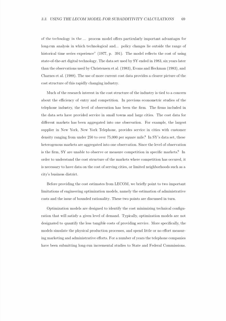
8/18/2019 Gasmi Cost Proxy Models
http://slidepdf.com/reader/full/gasmi-cost-proxy-models 69/318
3.3. USING THE LECOM MODEL FOR SUBADDITIVITY CALCULATIONS 69
of the technology in the ... process model offers particularly important advantages for
long-run analysis in which technological and... policy changes lie outside the range of historical time series experience” (1977, p. 391). The model reflects the cost of using
state-of-the-art digital technology. The data set used by SY ended in 1983, six years later
than the observations used by Christensen et al. (1983), Evans and Heckman (1983), and
Charnes et al. (1988). The use of more current cost data provides a clearer picture of the
cost structure of this rapidly changing industry.
Much of the research interest in the cost structure of the industry is tied to a concernabout the efficiency of entry and competition. In previous econometric studies of the
telephone industry, the level of observation has been the firm. The firms included in
the data sets have provided service in small towns and large cities. The cost data for
different markets has been aggregated into one observation. For example, the largest
supplier in New York, New York Telephone, provides service in cities with customer
density ranging from under 250 to over 75,000 per square mile.8 In SY’s data set, these
heterogenous markets are aggregated into one observation. Since the level of observation
is the firm, SY are unable to observe or measure competition in specific markets.9 In
order to understand the cost structure of the markets where competition has occured, it
is necessary to have data on the cost of serving cities, or limited neighborhoods such as a
city’s business district.
Before providing the cost estimates from LECOM, we briefly point to two important
limitations of engineering optimization models, namely the estimation of administrative
costs and the issue of bounded rationality. These two points are discussed in turn.
Optimization models are designed to identify the cost minimizing technical configu-
ration that will satisfy a given level of demand. Typically, optimization models are not
designated to quantify the less tangible costs of providing service. More specifically, the
models simulate the physical production processes, and spend little or no effort measur-
ing marketing and administrative efforts. For a number of years the telephone companies
have been submitting long-run incremental studies to State and Federal Commissions.
8/18/2019 Gasmi Cost Proxy Models
http://slidepdf.com/reader/full/gasmi-cost-proxy-models 70/318
70 CHAPTER 3. THE USE OF LECOM UNDER COMPLETE INFORMATION
In response to the charge that their process models did not incorporate these overhead
costs, the telephone companies have developed loading factors that take into account ad-ministrative and marketing expenses. Those loading factors have been included in our
model.10
Analytical properties of the LECOM cost function are difficult to determine outside
a direct experimental context. That is, it is not possible to know whether the cost
function is globally concave, which means that we do not know if the solution found by
our optimization model is a local or global minimum. Since there are an infinite number of possible configurations to be considered, and each proposed solution is costly to evaluate,
we limit our research to a reasonable number of possibilities. For each economically and
technically feasible combination of switches, we allow for up to 1000 possible iterations. An
iteration involves the calculation of the cost of service at one or more alternative locations
for the switches. For each market, and a given level of demand, LECOM evaluates a
number of different switch combinations. This further increases the number of solutions
that are evaluated. Therefore while this search process is not exhaustive, the model
considers a wide-range of feasible solutions.
3.4 Empirical Results
3.4.1 Measuring Economies of Scope
An industry is considered to be a natural monopoly if and only if a single firm can produce
the desired output at lower cost than any combination of two or more firms. This property,
known as subadditivity of the cost function, holds if for any set of goods N = {1, · · · , n}
and for any m output vectors Q1, · · · , Qm of goods in N : C (Q1) + C (Q2) + · · · + C (Qm) >
C (Q1 + Q2 · · · + Qm) (Baumol, 1977, p. 810). A necessary but not sufficient condition
for a natural monopoly is the presence of economies-of-scope. Economies of scope exist
if there is some exhaustive partitioning of the output space into nonintersecting subsets
and the cost of separately producing each subset exceeds the cost of producing all outputs
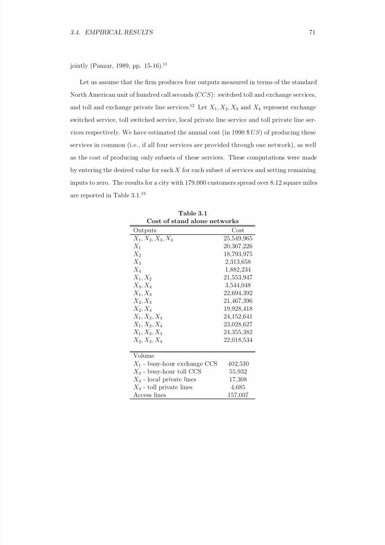
8/18/2019 Gasmi Cost Proxy Models
http://slidepdf.com/reader/full/gasmi-cost-proxy-models 71/318
3.4. EMPIRICAL RESULTS 71
jointly (Panzar, 1989, pp. 15-16).11
Let us assume that the firm produces four outputs measured in terms of the standard
North American unit of hundred call seconds (CCS ): switched toll and exchange services,
and toll and exchange private line services.12 Let X 1, X 2, X 3 and X 4 represent exchange
switched service, toll switched service, local private line service and toll private line ser-
vices respectively. We have estimated the annual cost (in 1990 $ US ) of producing these
services in common (i.e., if all four services are provided through one network), as well
as the cost of producing only subsets of these services. These computations were madeby entering the desired value for each X for each subset of services and setting remaining
inputs to zero. The results for a city with 179,000 customers spread over 8.12 square miles
are reported in Table 3.1.13
Table 3.1Cost of stand alone networks
Outputs Cost
X 1, X 2, X 3, X 4 25,549,965X 1 20,367,226X 2 18,793,975X 3 2,313,658X 4 1,882,234X 1, X 2 21,553,947X 3, X 4 3,544,048X 1, X 3 22,694,392X 2, X 3 21,467,396X 2, X 4 19,928,418X 1, X 3, X 4 24,152,641X 1, X 2, X 4 23,028,627X 1, X 2, X 3 24,355,382X 2, X 3, X 4 22,018,534
VolumeX 1 - busy-hour exchange CCS 402,530X 2 - busy-hour toll CCS 55,932X 3 - local private lines 17,308X 4 - toll private lines 4,685Access lines 157,007
8/18/2019 Gasmi Cost Proxy Models
http://slidepdf.com/reader/full/gasmi-cost-proxy-models 72/318
72 CHAPTER 3. THE USE OF LECOM UNDER COMPLETE INFORMATION
In order to determine the extent to which there are economies of scope, in Table 3.2,
we compare the cost of providing all four services on one network (C (X 1, X 2, X 3, X 4) =25, 549, 965), with the cost of providing the four services on two or more networks (see
column b).
Table 3.2(Dis)economies of scope
Multi-network offering* Stand-alone cost Degree of scope economies**(a) (b) (d)
C (X 1) + C (X 2, X 3, X 4) 42,385,760 0.658936C (X 2) + C (X 1, X 3, X 4) 42,946,616 0.680887C (X 3) + C (X 1, X 2, X 4) 25,342,285 -0.008130C (X 4) + C (X 1, X 2, X 3) 26,237,616 0.026914
C (X 1) + C (X 2) + C (X 3) + C (X 4) 43,357,093 0.696953C (X 1, X 2) + C (X 3, X 4) 25,097,995 -0.017690C (X 1, X 4) + C (X 2, X 4) 42,165,522 0.650316
C (X 1, X 2) + C (X 3) + C (X 4) 25,749,839 0.007823C (X 1, X 3) + C (X 2) + C (X 4) 43,370,601 0.697482C (X 1, X 4) + C (X 2) + C (X 3) 42,575,029 0.666344C (X 2, X 3) + C (X 1) + C (X 4) 42,947,586 0.680925C (X 2, X 4) + C (X 1) + C (X 3) 42,609,303 0.667685C (X 3, X 4) + C (X 1) + C (X 2) 42,705,249 0.671441
* The volumes X 1, X 2, X 3 and X 3 are those that are given at the bottom of Table 3.1 above.
** In this column, values greater than zero indicate economies of scope and values less than
zero indicate diseconomies of scope. This column (d) is computed according to the formula
(d) = ((b) − c)/c, where (b) refers to the column (b) containing the cost of stand-alone networks
and c is the cost of providing all services jointly, i.e., 25,549,965.
The first row of Table 3.2 shows that the total cost of providing exchange service
on one network C (X 1) and switched toll and private line services on a second network
C (X 2, X 3, X 4) is 42,385,760, which by Table 3.1 is equal to (20,367,226 + 22,018,534).
The cost of providing the four services on one network is 25,549,965. Consequently, the
ratio appearing in column (d) is greater than zero. When this ratio is greater than zero,
economies-of-scope are present. This indicates that it is more expensive to construct two
networks than to provide all four services on one network.
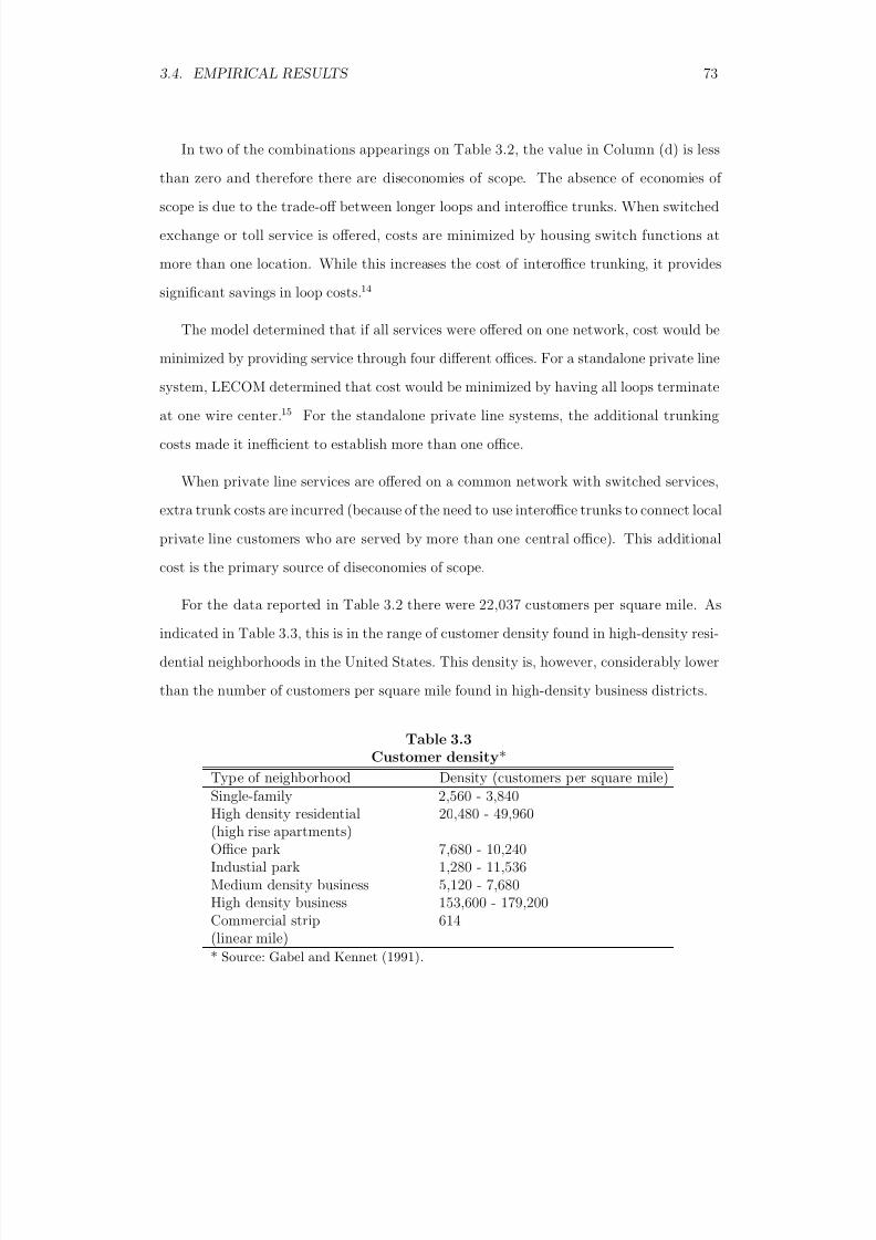
8/18/2019 Gasmi Cost Proxy Models
http://slidepdf.com/reader/full/gasmi-cost-proxy-models 73/318
3.4. EMPIRICAL RESULTS 73
In two of the combinations appearings on Table 3.2, the value in Column (d) is less
than zero and therefore there are diseconomies of scope. The absence of economies of scope is due to the trade-off between longer loops and interoffice trunks. When switched
exchange or toll service is offered, costs are minimized by housing switch functions at
more than one location. While this increases the cost of interoffice trunking, it provides
significant savings in loop costs.14
The model determined that if all services were offered on one network, cost would be
minimized by providing service through four different offices. For a standalone private linesystem, LECOM determined that cost would be minimized by having all loops terminate
at one wire center.15 For the standalone private line systems, the additional trunking
costs made it inefficient to establish more than one office.
When private line services are offered on a common network with switched services,
extra trunk costs are incurred (because of the need to use interoffice trunks to connect local
private line customers who are served by more than one central office). This additional
cost is the primary source of diseconomies of scope.
For the data reported in Table 3.2 there were 22,037 customers per square mile. As
indicated in Table 3.3, this is in the range of customer density found in high-density resi-
dential neighborhoods in the United States. This density is, however, considerably lower
than the number of customers per square mile found in high-density business districts.
Table 3.3Customer density*
Type of neighborhood Density (customers per square mile)Single-family 2,560 - 3,840High density residential 20,480 - 49,960(high rise apartments)Office park 7,680 - 10,240Industial park 1,280 - 11,536Medium density business 5,120 - 7,680High density business 153,600 - 179,200Commercial strip 614(linear mile)* Source: Gabel and Kennet (1991).
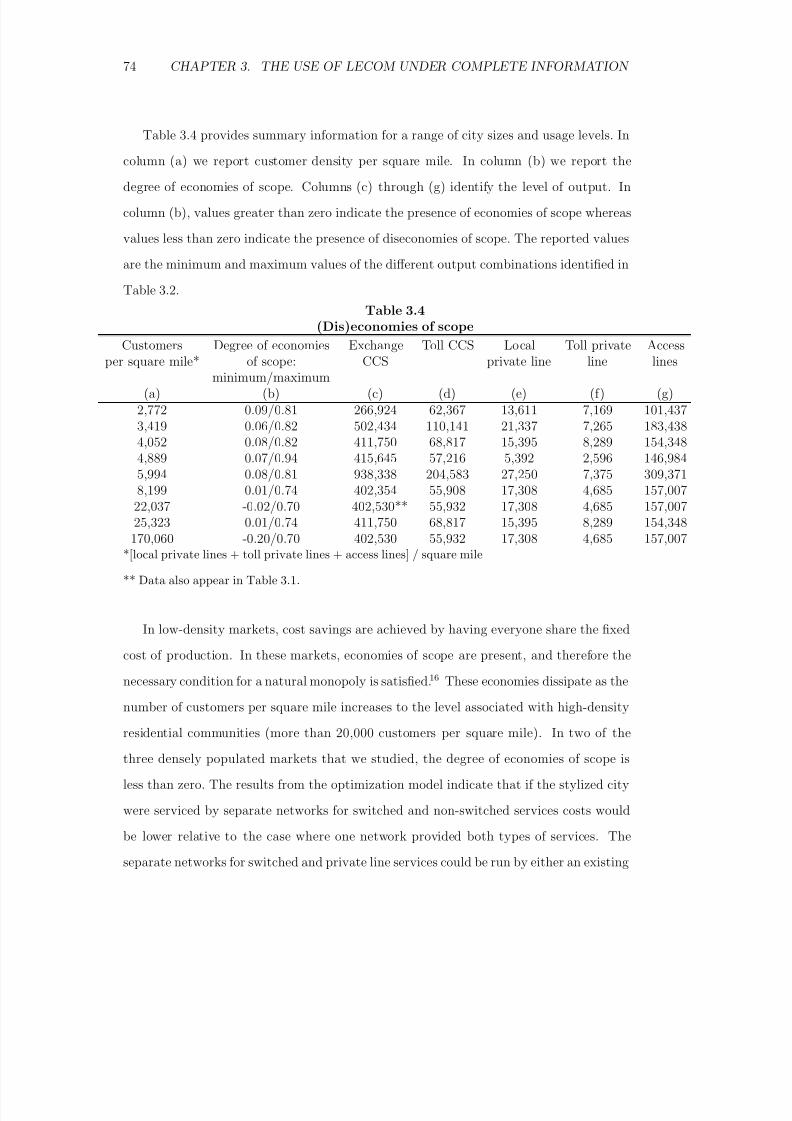
8/18/2019 Gasmi Cost Proxy Models
http://slidepdf.com/reader/full/gasmi-cost-proxy-models 74/318
74 CHAPTER 3. THE USE OF LECOM UNDER COMPLETE INFORMATION
Table 3.4 provides summary information for a range of city sizes and usage levels. In
column (a) we report customer density per square mile. In column (b) we report thedegree of economies of scope. Columns (c) through (g) identify the level of output. In
column (b), values greater than zero indicate the presence of economies of scope whereas
values less than zero indicate the presence of diseconomies of scope. The reported values
are the minimum and maximum values of the different output combinations identified in
Table 3.2.
Table 3.4
(Dis)economies of scopeCustomers Degree of economies Exchange Toll CCS Local Toll private Access
per square mile* of scope: CCS private line line linesminimum/maximum
(a) (b) (c) (d) (e) (f) (g)2,772 0.09/0.81 266,924 62,367 13,611 7,169 101,4373,419 0.06/0.82 502,434 110,141 21,337 7,265 183,4384,052 0.08/0.82 411,750 68,817 15,395 8,289 154,3484,889 0.07/0.94 415,645 57,216 5,392 2,596 146,9845,994 0.08/0.81 938,338 204,583 27,250 7,375 309,371
8,199 0.01/0.74 402,354 55,908 17,308 4,685 157,00722,037 -0.02/0.70 402,530** 55,932 17,308 4,685 157,00725,323 0.01/0.74 411,750 68,817 15,395 8,289 154,348
170,060 -0.20/0.70 402,530 55,932 17,308 4,685 157,007*[local private lines + toll private lines + access lines] / square mile
** Data also appear in Table 3.1.
In low-density markets, cost savings are achieved by having everyone share the fixed
cost of production. In these markets, economies of scope are present, and therefore thenecessary condition for a natural monopoly is satisfied.16 These economies dissipate as the
number of customers per square mile increases to the level associated with high-density
residential communities (more than 20,000 customers per square mile). In two of the
three densely populated markets that we studied, the degree of economies of scope is
less than zero. The results from the optimization model indicate that if the stylized city
were serviced by separate networks for switched and non-switched services costs would
be lower relative to the case where one network provided both types of services. The
separate networks for switched and private line services could be run by either an existing
8/18/2019 Gasmi Cost Proxy Models
http://slidepdf.com/reader/full/gasmi-cost-proxy-models 75/318
3.4. EMPIRICAL RESULTS 75
local exchange carrier or an entrant.
The results reported in Table 3.4 suggest that the likelihood of entry increases with
customer density. This is consistent with recent trends in the industry; entry has indeed
largely occurred in high-density nonresidential markets. Entry could be the result of one
or both of the following factors. First, in high density markets, the distance between the
customer and the telephone company’s office is relatively short compared to less dense
markets (New England Telephone, 1986, book 1, p. III. E.1.19). The cost of connecting a
customer to the office increases with the distance of that customer from the nearest facilityshared with other customers. If the lower cost of providing connections on short routes
is not reflected in the rates, subscribers in densely populated markets may be charged a
rate that exceeds the cost of service. The supra-competitive price would attract entry.
Second, an entrant may also be attracted to a densely populated market because of
the diseconomies of scope of the type of those that have been identified by LECOM. The
number of nodes on a network is determined by the number of customers served and
the size of the service territory. In densely populated markets, the incumbent telephone
companies provide service through multiple locations.
Entrants have found that because they serve a smaller number of customers than the
incumbent, and provide almost exclusively non-switched services (X 3 and X 4), produc-
tion costs are minimized by constructing a network with fewer nodes. For example, while
New York Telephone serves the area of Manhattan south of 96th Street with switching
machines at over 15 locations, an entrant, Teleport, serves the same territory with just
one node.17 We note that the incremental cost estimates we show here are similar to
those of Mitchell (1990) and those made by at least one industry participant (New Eng-
land Telephone, 1986). For example, for a roughly similar experiment involving a city
of about 40,000 lines, LECOM gives a loop cost estimate of about $113 per year (Gabel
and Kennet, 1991), while Mitchell shows about $104 and NET shows a range from $69 to
$156.
8/18/2019 Gasmi Cost Proxy Models
http://slidepdf.com/reader/full/gasmi-cost-proxy-models 76/318
76 CHAPTER 3. THE USE OF LECOM UNDER COMPLETE INFORMATION
3.4.2 Economies of Scope in Switched Services
The data reported in Table 3.5 below indicate that the degree of scope economies between
toll and exchange service is in the order of 0.8 for a large range of customer densities. To
a large degree, these economies of scope arise from the public input nature of the local
loop. Panzar defines joint goods as inputs “that are, once acquired for use in producing
one good, they are costlessly available for use in the production of others” (1989, p.17).
Local and toll usage on an access line during the peak hour is in the order of five minutes
(Rey, 1983, p.125). Once the loop is installed for a given service, the additional cost
of providing another service over the same facility is nil.18 If, on the other hand, local
and toll services are provided on separate networks, the non-trivial cost of the loop is
duplicated. In light of these intuitively clear strong economies of scope that derive from
the shared use of the local loop, there are reasons to be skeptical about SY’s finding that
for the products access lines, toll and exchange calls, the cost function is superadditive.
It should be noted that a potential shortcoming of the bottom-up modeling approach
is the failure to account for managerial economies and diseconomies. The bottom-up
method used here necessarily investigates costs at the level of the service area, while
managerial economies and diseconomies would occur at a super-regional level. One can
argue, however, that the evidence in the industry suggests that, if anything, there are
managerial economies of scale rather than diseconomies. For example, the number of
Regional Bell Operating Companies has dropped from seven after the breakup in 1984to four today. Several of these four, in turn, have either absorbed, or been absorbed by,
non-Bell companies. In 1985, according to the FCC there were 1518 study areas in the
United States. A study area represents the service area of a unique company operating
within a state. By 1999, this number had fallen to 1426. While both numbers actually
represent overestimates of the number of telephone companies operating within the U.S.,
the change together with anecdotal evidence clearly indicates that the total number of
companies has declined significantly in recent years. This fact suggests that management
believes it can operate most efficiently when the scale of operations is larger rather than
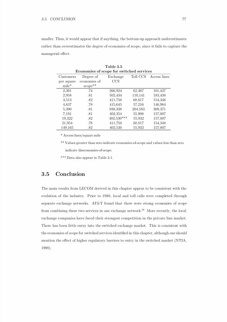
8/18/2019 Gasmi Cost Proxy Models
http://slidepdf.com/reader/full/gasmi-cost-proxy-models 77/318
3.5. CONCLUSION 77
smaller. Thus, it would appear that if anything, the bottom-up approach underestimates
rather than overestimates the degree of economies of scope, since it fails to capture themanagerial effect.
Table 3.5Economies of scope for switched services
Customers Degree of Exchange Toll CCS Access linesper square economies of CCS
mile* scope**2,301 .74 266,924 62,367 101,437
2,958 .81 502,434 110,141 183,4383,513 .82 411,750 68,817 154,3484,637 .78 415,645 57,216 146,9845,390 .81 938,338 204,583 309,3717,191 .81 402,354 55,908 157,007
19,322 .82 402,530*** 55,932 157,00721,954 .78 411,750 68,817 154,348
149,165 .82 402,530 55,932 157,007
* Access lines/square mile
** Values greater than zero indicate economies-of-scope and values less than zero
indicate diseconomies-of-scope.
*** Data also appear in Table 3.1.
3.5 Conclusion
The main results from LECOM derived in this chapter appear to be consistent with theevolution of the industry. Prior to 1980, local and toll calls were completed through
separate exchange networks. AT&T found that there were strong economies of scope
from combining these two services in one exchange network.19 More recently, the local
exchange companies have faced their strongest competition in the private line market.
There has been little entry into the switched exchange market. This is consistent with
the economies of scope for switched services identified in this chapter, although one should
mention the effect of higher regulatory barriers to entry in the switched market (NTIA,
1988).

8/18/2019 Gasmi Cost Proxy Models
http://slidepdf.com/reader/full/gasmi-cost-proxy-models 78/318
78 CHAPTER 3. THE USE OF LECOM UNDER COMPLETE INFORMATION
One policy implication of the study described in this chapter is that regulatory over-
sight of the incumbents’ pricing of local network access in the presence of private lineservice may be problematic. The question of a proper allocation of cost between these
two services which share a large portion of the network infrastructure can be addressed
using LECOM, but regulators must be aware of the appropriate methodology for such
an allocation (see Sharkey, 1982). At times when faced with entry, the local exchange
companies have adopted rates that were based on the cost structure of their competitors
(Temin, 1990, p.353). If the incumbents continue to use one network for both switched
and non-switched services, regulatory commissions should set the incumbents’ rates for
private line services based on the marginal cost of production of the existing network
architecture.
While there are diseconomies of scope in part of the local exchange market, the
LECOM calculation approach departs from SY in the measurement of their magnitude.
This approach does not yield “considerable” (SY, 1992, p. 181) diseconomies of scope.
Consequently, the larger gains expected from competition are most likely to arise from
the dynamic incentives of rivalry rather than static diseconomies of scope.

8/18/2019 Gasmi Cost Proxy Models
http://slidepdf.com/reader/full/gasmi-cost-proxy-models 79/318
NOTES 79
Notes
1This chapter is based on Gabel and Kennet (1994). We thank David Gabel for his
permission to use the material.
2See Section 3.4.1 for a definition.
3Leggette (1985) has also used the translog cost function and data from the Statistics
of Common Communication Carriers to estimate a multiproduct cost function. Leggette
concluded that there were no economies of scope between the two outputs he considered
in his study, private branch exchange and main station telephones.
4When Christensen, Cummings and Schoech (1981) built the data set that has been
used by prior econometricians, they used different price indexes for each of the primary
types of facilities.
5For example, between 1976 and 1980, the price of outside plant increased by 33 %,
while inside plant increased by 12 % (Bell System Telephone Plant Indexes).
6See Rey (1983, p.125). In standard traffic engineering terminology, this level of peak
usage corresponds to 0.125 Erlang or 3 C CS . In this example, we treat usage as the sum
of exchange and toll usage. This simplification does not affect our analysis.
7See ”Usage Forecasting by Class of Service”, American Telephone and Telegraph Sys-
tem Letter , 83-05-128.
8Response of New York Telephone to User Request #147 , Case 28978, New York Public
Service Commission.
9The data set used by Christensen, Cummings and Schoech (1983), Evans and Heck-
man (1983), and Charnes et al. (1988) suffers from the same problem.
10To be somewhat more specific, administrative costs are a linear function of the level of
investment. Therefore, the administrative costs will exhibit the same economies or disec-

8/18/2019 Gasmi Cost Proxy Models
http://slidepdf.com/reader/full/gasmi-cost-proxy-models 80/318
80 NOTES
onomies that are present in the use of physical facilities. Evans and Heckman (1983, p.141)
raise the issue of whether managerial diseconomies can exceed engineering economies. Be-cause of this concern, they argue that “Although engineering studies may be useful to
businessmen choosing between alternative technologies, they are of little use for deter-
mining whether an industry is a natural monopoly.” Evans and Heckman express their
preference for “hard data” rather than engineering constructs. (Ibid., p. 141). Unfortu-
nately, the “hard data” approach provides little or no indication on the industry’s current
or future cost trends. In order to identify prospective costs, in a dynamic, capital intensive
industry, we believe that data generated through an optimization model provides more
insights than “hard” but historical data.
11Sufficient conditions for a multiproduct natural monopoly are economies of scope and
declining average incremental costs (see Evans and Heckman 1984, pp. 615-16). Other
sufficient conditions for a natural monopoly are discussed in Sharkey (1982), pp. 67-73.
12
Whenever toll or exchange switched service is provided, the customer is connected to
the switch via an access line. While this cost is included in the tables below, here we do
not list it as a product by itself.
13See Chapter 2 for the shape of the generic city which is assumed in LECOM.
14The diseconomies of scope occur between switched services on one hand and private
line networks on the other. Since both networks build a trunk to an interoffice POP
(see Section 2.3.4 of Chapter 2), interconnection is already included in the cost, and the
diseconomies arise purely because of the fact that the model “forces” the firm in providing
the private line network to use the same infrastructure used for the switched plant. In
practice, these diseconomies might disappear because a single firm can mimic the two-firm
solution modeled by LECOM.
15No switching costs are incurred with an all private line system.
16We have not tested for the sufficient conditions of a natural monopoly (see footnote
8/18/2019 Gasmi Cost Proxy Models
http://slidepdf.com/reader/full/gasmi-cost-proxy-models 81/318
NOTES 81
12).
17New York Telephone response to information request CPBCS 199, in Docket 28978,
New York Public Service Commission.
18Within the industry, the cost attributes commonly allocated to the local loop are
non-traffic sensitive. The nomenclature reflects a situation with no congestion in the
local loop.
19
Memorandum from T. Sheridan to J. Hudson (November 20, 1895), box 1275, Amer-ican Telephone and Telegraph Corporate Archive.

8/18/2019 Gasmi Cost Proxy Models
http://slidepdf.com/reader/full/gasmi-cost-proxy-models 82/318
82 NOTES
8/18/2019 Gasmi Cost Proxy Models
http://slidepdf.com/reader/full/gasmi-cost-proxy-models 83/318
Chapter 4
Regulation under Incomplete
Information
4.1 Introduction
The new economics of regulation has stressed the role of asymmetric information be-
tween regulators and regulated firms, in particular, asymmetric information about cost
functions.1 Before explaining in Chapter 5 how asymmetric information is introduced
in the engineering model described in Chapter 2, we present in this chapter a canoni-
cal model of regulation that will constitute the central theoretical basis of the empirical
analyses conducted in this book.
In Section 4.2 we describe the basic theoretical model we will be using throughout the
remaining chapter. This regulation model of a telecommunications monopoly is borrowed
from Laffont and Tirole (1986). The production cost of the regulated good depends
on an efficiency characteristic which is private information of the regulated firm and on
a level of effort which decreases cost but creates a disutility for the firm’s managers.
The complete information benchmark is also derived in this section. In this complete
information scheme, the marginal disutility of effort equates the marginal cost saving, the
price of the regulated good equates the social marginal cost and no rent is left to the firm.
Optimal regulation under incomplete information when cost is observable ex post is
characterized in Section 4.3. Asymmetric information obliges the regulator to give up an
83
8/18/2019 Gasmi Cost Proxy Models
http://slidepdf.com/reader/full/gasmi-cost-proxy-models 84/318
84 CHAPTER 4. REGULATION UNDER INCOMPLETE INFORMATION
information rent to efficient firms. This rent is socially costly since it must be financed
with distortive taxes and the regulator wishes to decrease it. To do so the regulatoraccepts some distortions. First, it offers a menu of cost-reimbursement rules among which
firms self-select themselves according to their type. These rules induce underprovisions of
effort relative to the complete information allocations. Second, pricing is made according
to the Ramsey rule with two corrections: an incentive correction may be added to the
Ramsey pricing formula (under some conditions on the cost function this correction is
not needed) and the marginal cost in the Ramsey rule is evaluated at the effort level
induced by the cost-reimbursement rule and not the complete information effort level.
The ex post observability of cost requires proper auditing which may not be available
or which may be too costly and regulation must then be designed in the absence of cost
observability. Section 4.4 derives optimal regulation in the absence of cost observability.
In this case, regulation has only one instrument, namely pricing, to decrease the socially
costly information rents which must be given up to the efficient types. Distortion of
pricing, and therefore of the production level, with respect to Ramsey pricing is then
always needed.
The two types of regulation characterized in Sections 4.3 and 4.4 use transfers from
the regulator to the firm. These transfers could alternatively come from consumers in the
form of the fixed fees of two-part tariffs; then, the social distortions would not arise from
the distortive financing of the transfers, but from the costly disconnections of those who
would not find worthwhile to pay the fixed fees. We do not derive this type of regulation
which requires a delicate modeling of consumers’ behavior, but instead we characterize in
Section 4.5 several variants of price-cap regulation which is a regulation without transfers
and without cost observability. A simple cap on prices makes the firm residual claimant for
its cost saving and induces an effort level which is efficient conditionally on the quantity
produced. However, it yields high rents to the efficient types. This very common regula-
tory rule is sometimes complemented by taxation of the firm’s profit (in which case cost
observability is again assumed). This approach decreases profits and therefore incentives
8/18/2019 Gasmi Cost Proxy Models
http://slidepdf.com/reader/full/gasmi-cost-proxy-models 85/318
4.2. THE MODEL 85
for cost minimization, but enables the regulator to decrease the information rents.
Finally, in Section 4.6 the traditional cost-plus regulation is characterized. Under this
scheme, the firm which is fully reimbursed for its costs has no incentive to minimize them.
Effort is minimal and efficiency low. However, the regulator is then able to eliminate
information rents. To mitigate the distortions due to the balanced budget condition
implicit in cost-plus regulation, the regulator may complement the revenues of the firm
with costly transfers. This cost-plus regulation with transfers is also considered in this
section.
4.2 The Model
We consider a single-product regulated firm with aggregate cost function
C = C (β, e, q ) (4.1)
where β is a technological parameter or firm’s type, with C β > 0, e is its managers’
cost-reducing effort, with C e < 0, q is the firm’s output level, with C q > 0 and C qq < 0.
We denote E (β, C , q ) the effort required for a firm of type β to produce q at cost C .
By definition
C = C (β, E (β, C , q ), q ). (4.2)
First, we assume that cost is ex post observable and we make the accounting convention
that cost is reimbursed by the regulator to the firm and that the revenue R(q ) generated
by the sale of outputs is received by the regulator.
Letting t denote the net monetary transfer2 from the regulator to the firm and ψ the
disutility of effort for the firm’s managers (with ψ(0) = 0, ψ > 0, ψ < 0), the objective
function of the firm is
U = t − ψ(e). (4.3)

8/18/2019 Gasmi Cost Proxy Models
http://slidepdf.com/reader/full/gasmi-cost-proxy-models 86/318
86 CHAPTER 4. REGULATION UNDER INCOMPLETE INFORMATION
The firm is willing to participate in the regulatory process if and only if its participation
constraint is satisfied, i.e., here
U ≥ 0. (4.4)
Let 1 + λ (> 1) denote the social value of public funds. If S (q ) is the gross consumer
surplus attached to the consumption of telecommunications goods q , the social value of
q , denoted V (q ), is equal to the sum of the net consumer surplus, S (q ) − R(q ), and of the
social value from the sales of the goods, (1 + λ)R(q ). That is,
V (q ) = S (q ) + λR(q ). (4.5)
This social value of production is composed of the utility of the good supplemented by
the fiscal value of revenues, i.e., the decrease of tax distortions allowed by these revenues.
In particular, for linear prices such that R(q ) = P (q )q , where P (·) is the inverse demand
function,
V (q ) = S (q ) + λP (q )q. (4.6)
Consumers’ welfare (CW ) equals the utility of the good minus the costs which include
the real cost C and the transfer to the firm t evaluated at the social value of public funds,
namely,
CW = V (q ) − (1 + λ)(t + C (β, e, q )). (4.7)
The utilitarian social welfare function is the sum of the consumers’ welfare and the
firm’s welfare, i.e.,
W = [V (q ) − (1 + λ)(t + C (β, e, q ))] + U (4.8)
= V (q ) − (1 + λ)(C (β, e, q ) + ψ(e)) − λU. (4.9)
From the expression (4.9) of the social welfare function we see that it is costly to give
up rents (U > 0) to the firm. Under complete information this does not happen. Then,
8/18/2019 Gasmi Cost Proxy Models
http://slidepdf.com/reader/full/gasmi-cost-proxy-models 87/318
4.3. OPTIMAL REGULATION UNDER INCOMPLETE INFORMATION... 87
maximizing social welfare under the firm’s participation constraint (4.4) yields:
ψ(e) = −C e(β, e, q ) (4.10)
V (q ) = (1 + λ)C q(β, e, q ) (4.11)
t = ψ(e) or U = 0. (4.12)
The marginal disutility of effort is equated to the marginal cost saving of effort ((4.10)).
The marginal social valuation of production is equated to the marginal social cost of
production ((4.11)). As the regulator is fully informed, he leaves no rent to the firm in
order to save on the tax distortions ((4.12)).
Under complete information this optimal allocation can be implemented in various
ways with cost plus schemes, price-caps or more general cost sharing rules.
4.3 Optimal Regulation under Incomplete Informa-tion with Cost Observability
Regulation takes place now under incomplete information. The regulator observes neither
β nor e, which are known by the firm. The regulator must design regulation without
knowing the cost characteristic β . He is modeled as a Bayesian statistician who has
a prior probability distribution on β and who maximizes expected social welfare. We
assume thus that it is common knowledge that β is drawn from a cumulative distribution
function
3
F (·) on [β, ¯β ] with a density function f (β ) > 0 for any β .
For simplicity of exposition, we assume that no type is ever shut-down in the solutions
of the various programs below, i.e, the social value of production is so high that the firm
must be active whatever its cost characteristics.
We model regulation as a revelation mechanism4
q (β ), C (β ), t(β ) (4.13)
which specifies, for each announcement β , a production level to realize, a cost target to
meet and a net transfer from the regulator.

8/18/2019 Gasmi Cost Proxy Models
http://slidepdf.com/reader/full/gasmi-cost-proxy-models 88/318
88 CHAPTER 4. REGULATION UNDER INCOMPLETE INFORMATION
The utility level of a β -firm claiming that it is of type β is
U (β, β ) = t(β ) − ψ(E (β, C (β ), q (β ))). (4.14)
Truthful revelation of the cost characteristic β or incentive compatibility amounts to
t(β ) − ψ(E (β, C (β ), q (β ))) ≥ t(β ) − ψ(E (β, C (β ), q (β ))) (4.15)
for all (β, β ). In other words, β = β must maximize U (β, β ), i.e., for a differentiable
mechanism5,6,
t(β ) = ψ (e)
E C C (β ) + E q q (β )
. (4.16)
Let U (β ) denote firm β ’s utility level when it tells the truth, i.e, U (β ) = U (β, β ).
From the envelope theorem7, the first-order incentive compatibility condition is8
˙U (β ) = −ψ
(e)E β (β, C (β, e, q ), q ). (4.17)
So, incentive theory characterizes with (4.17) the additional constraints put by asymmetric
information on the allocation of resources. The regulator who does not know β behaves
as a Bayesian statistician and maximizes expected social welfare under the participation
constraints (4.4) and the new incentive constraints (4.17), i.e., solves
max{q(·),e(·),U (·)} E β W = β
β [V (q (β )) − (1 + λ)(C (β, e(β ), q (β )) + ψ(e(β )) − λU (β )] f (β )dβ (4.18)
s.t. (4.4) and (4.17). The first-order conditions of this program9 are
ψ(e) = −C e − λ
1 + λ
F (β )
f (β )
d
de(ψ(e)E β ) (4.19)
V (q ) = (1 + λ)C q + λF (β )
f (β )ψ(e)
d
dq E β . (4.20)
Equation (4.19) refers to the cost-reimbursement rule imbedded in optimal regulation.
Let us see why. When the firm is residual claimant for its cost savings due to effort, the

8/18/2019 Gasmi Cost Proxy Models
http://slidepdf.com/reader/full/gasmi-cost-proxy-models 89/318
4.3. OPTIMAL REGULATION UNDER INCOMPLETE INFORMATION... 89
firm equates the marginal disutility of effort, ψ(e), to marginal cost saving, −C e. I f a
share α of its cost is reimbursed, the firm solves
mine
[ψ(e) + (1 − α)C (β, e, q )], (4.21)
i.e.,
ψ(e) = −(1 − α)C e. (4.22)
Therefore, in (4.19),
λ1 + λ
F (β )f (β )
dde (ψ(e)E β )
(−C e) (4.23)
can be interpreted as the share α of costs reimbursed to the type β firm.
The share 1 − α represents the power of the incentive scheme. Indeed, if α = 0, the
firm is residual claimant of its cost savings and chooses the level of effort which is first
best conditionally on the level of output. It is a “high-powered incentive scheme”. If
α = 1, the whole monetary cost is reimbursed to the firm and there is no incentive for
effort. It is a “low-powered incentive scheme”.
Equation (4.20) describes optimal pricing. For linear pricing R(q ) = P (q )q and
V (q ) = S (q ) + λ[P (q )q + P (q )]. (4.24)
Noting that S (q ) = p we have the Lerner index formula:
p − C q
p = λ
1 + λ
1
η + λ
1 + λ
F (β )
f (β )
ψ(e)
p
d
dq E β (4.25)
or
L = R + I (4.26)
where η is the price elasticity of demand. We thus obtain a modified Ramsey pricing rule
in which the Lerner index, L = ( p − C q)/p, equals the inverse price elasticity of demand
times λ/(1 + λ), R = (λ/(1 + λ))(1/η), to which an incentive correction I given by
I = λ
1 + λ
F (β )
f (β )
ψ(e)
p
d
dq E β (4.27)

8/18/2019 Gasmi Cost Proxy Models
http://slidepdf.com/reader/full/gasmi-cost-proxy-models 90/318
90 CHAPTER 4. REGULATION UNDER INCOMPLETE INFORMATION
is added.
In general, incentive considerations affect pricing. Let us see why. We can integrate
equation (4.17) to obtain the information rent of a type β form (using the fact that
U (β ) = 0, since rents are costly to the regulator)
U (β ) =
β
β
ψ(e(b))E β (b, C (b, e(b), q (b)), q (b))db. (4.28)
Contrary to the situation of complete information, the regulator is now obliged to give
up this rent which is socially costly.10 He will then want to decrease it. From (4.28)
this is possible by decreasing e(β ) to decrease ψ(e(β )) and also by more sophisticated
distortions involving also q (β ) and therefore pricing when E β is a function of q (·).
A dichotomy between pricing and incentives occurs when the incentive correction
vanishes, i.e., when
d
dq E β ≡ 0, (4.29)
i.e., when
C = C (Φ(β, e), q ) (4.30)
by the Leontief theorem.11 When the rate E β at which the firm can substitute a decrease
of effort to an increase of β , (which affects how the information rent must decrease with
β for incentive reasons (see 4.28)), is independent of the production level, it is useless
to distort the production level to decrease the information rent. This benchmark case of
dichotomy is interesting for its simplicity and we will investigate empirically whether it
can be viewed as a reasonable approximation for the true cost function.12
Optimal regulation with cost observability will be referred to as LT regulation from
Laffont-Tirole (1986).
8/18/2019 Gasmi Cost Proxy Models
http://slidepdf.com/reader/full/gasmi-cost-proxy-models 91/318
4.4. OPTIMAL REGULATION WITHOUT COST OBSERVABILITY 91
4.4 Optimal Regulation without Cost Observability
When cost is not observable and therefore cannot be reimbursed, the firm has always the
incentive to choose the optimal effort level given its type and production level, i.e.,
ψ(e) = −C e(β, e, q ). (4.31)
Letting e∗(β, q ) denote the solution of (4.31), the firm’s objective function is now:
U (β ) = t(β ) − C (β, e∗(β, q (β )), q (β )) − ψ(e∗(β, q (β ))). (4.32)
Following the same steps as in the previous section, we can derive the incentive constraint
which, from the envelope theorem, writes now as:
U (β ) = −C β (β, e∗(β, q (β )), q (β )). (4.33)
The regulator’s program becomes
maxq(·),U (·)
β
β
[V (q (β )) − (1 + λ) (C (β, e∗(β, q (β )), q (β )) + ψ(e∗(β, q (β ))) − λU (β )] f (β )dβ
(4.34)
s.t. (4.33) and U (β ) ≥ 0 for any β . The first order condition of this program is:
V (q ) = (1 + λ)C q + λF (β )
f (β )C βq (4.35)
or, for linear pricing,
p − C q
p
= λ
1 + λ
1
η
+ λ
1 + λ
F (β )
f (β )
C βq
p
. (4.36)
Without cost observability we have lost one instrument and the distortion of the
pricing rule away from Ramsey pricing is now the only way to decrease the information
rent. Indeed, from (4.33) the information rent is:
U (β ) =
β
β
C β (b, e∗(b, q (b)), q (b))db (4.37)
and only a distortion of q (·) can affect it.
The optimal regulation without cost observability will be referred to as BM regulation
from Baron-Myerson (1982).

8/18/2019 Gasmi Cost Proxy Models
http://slidepdf.com/reader/full/gasmi-cost-proxy-models 92/318
92 CHAPTER 4. REGULATION UNDER INCOMPLETE INFORMATION
4.5 Price-Cap Regulation
Price-cap regulation is a regulation without cost observability and without transfer. Let
q ( p) be the demand function. Let us denote by pM (β ) the profit-maximizing price asso-
ciated with the optimal effort level, that is, the solution in p of
maxe,p
pq ( p) − C (β, e, q ( p)) − ψ(e). (4.38)
The first-order conditions of (4.38) can readily be seen to be13
ψ(e) = −C e(β, e, q ( p)) (4.39)
and
p − C q(β, e, q ( p)) = − q ( p)
dq
dp( p)
, or p − C q
p =
1
η, (4.40)
the latter being the classical monopoly pricing formula. Under appropriate assumptions
on the aggregate cost function (C ee > 0, C βe > 0, C eq < 0 and C βq > 0) it can be shown, by
using a standard revealed-preference argument, that the monopoly price is nondecreasing
in β . A regulatory solution with a price-cap ¯ p gives the monopoly price pM (β ) for β less
than or equal to some β ∗ and ¯ p for β > β ∗ (see Figure 4.1).14
¯ p
β β ∗ β β
pM (β )
pM (β )
( pM (β ∗))
pM
Figure 4.1: Price-cap with downward price flexibility

8/18/2019 Gasmi Cost Proxy Models
http://slidepdf.com/reader/full/gasmi-cost-proxy-models 93/318
4.5. PRICE-CAP REGULATION 93
So, the optimal price-cap regulation in this simple example with a single price is
obtained by finding the optimal value β ∗
or the optimal ¯ p under the condition that theleast efficient firm (type β ) does not make negative profit, i.e, the optimal price-cap
regulation solves
max¯ p
β ∗
β
[S (q ( pM (β ))) − C (β, e∗(β, q ( pM (β ))), q ( pM (β )))
−ψ(e∗(β, q ( pM (β ))))]f (β )dβ
+
β
β ∗[S (q (¯ p)) − C (β, e∗(β, q (¯ p)), q (¯ p))
−ψ(e∗(β, q (¯ p)))]f (β )dβ (4.41)
under the participation constraint of the least efficient firm:
¯ pq (¯ p) − C (β, e∗(β, q (¯ p)), q (¯ p)) − ψ(e∗(β, q (¯ p))) ≥ 0. (4.42)
Two regimes are possible a priori, according to whether or not the constraint (4.42) is
binding. With C qq < 0, this constraint is binding. Suppose it is not. Then q (¯ p) maximizes
(4.41) without constraint. Using (4.39), the first-order condition is β
β ∗[S (q (¯ p)) − C q(β, e∗(β, q (¯ p)), q (¯ p)]f (β )dβ = 0, (4.43)
or using ¯ p = S (q (¯ p))
¯ p =
β
β ∗C q(β, e∗(β, q (¯ p)), q (¯ p))f (β )dβ
1 − F (β ∗) . (4.44)
Since C qβ > 0, C qe < 0 and ∂e∗/∂β > 0, (4.44) implies ¯ p ≤ C q(β, e∗(β, q (¯ p)), q (¯ p)) which
gives a contradiction of (4.42) since C qq < 0.15 We will therefore solve for ¯ p from (4.42)
above to obtain the optimal price-cap regulation in which β ∗ is defined by pM (β ∗) =
¯ p, when the regulator wants the firm to be active whatever its type in [β, β ]. This
mechanism corresponds to an optimal price-cap regulation without transfers and without
cost observability. It is designated by PC in the book.
The excessive profits associated with (pure) price-cap regulation have sometimes led
regulators to append to it a profit-sharing rule.16 The firm’s financial profit net of taxes
8/18/2019 Gasmi Cost Proxy Models
http://slidepdf.com/reader/full/gasmi-cost-proxy-models 94/318
94 CHAPTER 4. REGULATION UNDER INCOMPLETE INFORMATION
(at a rate τ ) is then given by17
(1 − τ )[ pq ( p) − C (β, e∗(β, q ( p)), q ( p))]. (4.45)
The price-cap ¯ p is again determined by the individual rationality constraint of the least
efficient firm β ,
(1 − τ )[¯ pq (¯ p) − C (β, e(β, q (¯ p), τ ), q (¯ p))] − ψ(e(β, q (¯ p), τ )) = 0, (4.46)
where e(β, q (¯ p), τ ) is defined as the solution to
ψ(e) = (1 − τ )C e(β, e, q (¯ p)). (4.47)
Let ¯ p(τ ) be the solution obtained from (4.46) and (4.47), and pM (β, τ ) the monopoly
price under profit sharing. Note that if the revenue from taxing the firm is used to decrease
taxes elsewhere in the economy18, then it has net social value
λτ β ∗
β [ pM
(β, τ )q ( pM
(β, τ )) − C (β, e( pM
(β, τ )), q ( pM
(β, τ )))]f (β )dβ
+
β
β ∗[¯ p(τ )q (¯ p(τ )) − C (β, e(β, q (¯ p(τ ))), q (¯ p(τ )))]f (β )dβ
. (4.48)
The optimal sharing rule then solves
maxτ
β ∗
β
[S (q ( pM (β, τ ))) − (1 + λτ )C (β, e(β, q ( pM (β, τ ))), q ( pM (β, τ )))
+λτ pM (β, τ )q ( pM (β, τ )) − ψ(e(β, q ( pM (β, τ ))))]f (β )dβ
+ β
β ∗[S (q (¯ p(τ ))) − (1 + λτ )C (β, e(β, q (¯ p(τ ))), q (¯ p(τ )))
+λτ ¯ p(τ )q (¯ p(τ )) − ψ(e(β, q (¯ p(τ ))))]f (β )dβ
, (4.49)
where β ∗ is defined by pM (β ∗, τ ) = ¯ p(τ ).
The particularly interesting feature of price-cap regulation with taxation of earnings
(called PCT) is the simplicity and practicability of the mechanism. However, it presumes
the observability of profits, which is equivalent to the observability of costs if revenues
are observable as we have assumed so far, and uses one-way transfers, i.e., taxes but not
8/18/2019 Gasmi Cost Proxy Models
http://slidepdf.com/reader/full/gasmi-cost-proxy-models 95/318
4.6. COST-PLUS REGULATION 95
subsidies. Conditionally on these informational or institutional constraints, it is not an
optimal mechanism, because expected social welfare could be improved by using a menuof price-cap/tax rates or by making a better use of cost observability.
It is worthwhile to note that the quality of price-cap mechanisms, which is a mechanism
without transfers contrary to LT and BM, is related to the size of the fixed costs. As fixed
costs increase, pricing is more and more distorted away from optimal Ramsey pricing to
cover costs and disutility of effort.
4.6 Cost-Plus Regulation
Under cost-plus regulation the regulator is again assumed to observe costs ex post and
to fully reimburse the firm for them. We will first consider the case where no additional
transfers to the firm are made, i.e., a balanced-budget constraint is imposed. This regula-
tory scheme, called C +, will be thought of as a formal representation of standard cost-plusregulation. Since the firm’s utility is then given by −ψ(e), the profit-maximizing firm can
be assumed to choose the minimum level of effort (emin = 0), which gives zero disutility.
In this case, the regulator imposes a production level q (β ) that solves
P (q (β ))q (β ) − C (β, 0, q (β )) = 0, (4.50)
leading to expected social welfare given by β
β
[S (q (β )) − C (β, 0, q (β ))]f (β )dβ. (4.51)
Alternatively, one could consider the case where, after collecting revenues, the regula-
tor gives to the firm a net transfer T = C (β, 0, q (β )) − P (q (β ))q (β ), which can be used to
ensure that the firm’s budget is balanced ex post . Since the firm has its cost reimbursed,
it is indifferent to the level of output. Under this scheme called C + T , the regulator
can therefore instruct the firm to produce the level q (β ) that maximizes expected social

8/18/2019 Gasmi Cost Proxy Models
http://slidepdf.com/reader/full/gasmi-cost-proxy-models 96/318
96 CHAPTER 4. REGULATION UNDER INCOMPLETE INFORMATION
welfare given by
¯β
β
[S (q (β )) − P (q (β ))q (β ) − (1 + λ)T ]f (β )dβ
=
β
β
[V (q (β )) − (1 + λ)C (β, 0, q (β ))]f (β )dβ. (4.52)
4.7 Remark
In the Laffont-Tirole (1986) model described above, the disutility of effort which decreases
the monetary cost has the nature of a fixed cost. One might want to extend the model
to cases where the disutility of effort depends on the level of production, i.e., when it can
be written as ψ(e, q ).
Following the same steps as above, we have now
U = t − ψ(e, q ) (4.53)
W = V (q ) − (1 + λ)(C (β, e, q ) + ψ(e, q )) − λU (4.54)
Under the assumption that C (β, e, q ) + ψ(e, q ) is convex in (e, q ), optimal regulation is
characterized by the first-order conditions
ψ(e) = −C e − λ
1 + λ
F
f
d
de(ψeE β ) (4.55)
V (q ) = (1 + λ)(C q + ψq) + λF
f
d
dq
(ψeE β ). (4.56)
A noticeable difference with the analysis above is the condition for the incentives-
pricing dichotomy to hold which now is expressed as:
d
dq [ψeE β ] = 0 (4.57)
It is natural to look for independent conditions on the cost function and on the disutil-
ity of effort function to obtain (4.57). We need the same condition on the cost function as
before (i.e. when ψ is independent of q ), which ensures that d
dq E β = 0, and then we must
8/18/2019 Gasmi Cost Proxy Models
http://slidepdf.com/reader/full/gasmi-cost-proxy-models 97/318
4.7. REMARK 97
have ψeq = 0. With the normalization ψ(0, q ) = 0 for all q , we are back to the original
Laffont-Tirole formulation. So, we cannot expect the incentives-pricing dichotomy to holdwhen the disutility of effort depends on the production level unless the terms in q of ψe
and E β cancel out which is, in general, very unlikely to occur.
Pursuing this latter strategy is not very attractive since we do not have enough prior
information on ψ(e, q ) in order to make interesting the characterization of cost functions
such that (4.57) holds for particular specifications of ψ(e, q ). Nevertheless, in Chapter 6,
leaving out the dichotomy property we will test the robustness of the other features of optimal regulation for the case ψ(e, q ) = ϕ(e)q .

8/18/2019 Gasmi Cost Proxy Models
http://slidepdf.com/reader/full/gasmi-cost-proxy-models 98/318
98 NOTES
Notes
1See Laffont (1994) for a survey of this literature and Laffont and Tirole (2000) for a
non-technical exposition. For a more technical presentation of the basic concepts and yet
at a relatively elementary level, the reader might find it useful to go through Chapter 1
of Laffont and Tirole (1993), in particular, Section 1.3 of that chapter.
2The gross transfer t would be such that t = t + R(q ) − C .
3
To avoid regulatory solutions with bunching we make the monotone hazard rate as-sumption
d
dβ
F (β )
f (β )
> 0 for all β.
Without fear of confusion, we denote with C both the cost function C (β, e, q ) and the
argument C (β ) of the revelation mechanism.
4Without loss of generality because of the Revelation Principle (Gibbard (1973), Green
and Laffont (1977) and Myerson (1979)), any regulation mechanism is equivalent to a
truthful revelation mechanism.
5From now on, we make the arguments of functions explicit only when it is needed for
clarity. Derivatives with respect to β of functions which are only functions of β will be
denoted with dots, i.e., t(β ), q (β ), C (β ), U (β ).
6From (4.14), we see that a necessary condition for truthful behavior (i.e. for β = β
to be an optimal announcement or U (β, β ) to be maximized with respect to β ) is the first
order condition of the maximization of U (β, β ) with respect to β .
7From (4.16), U β (β, β )/β =β = 0 for any β, β or U β (β, β ) = 0 for any β . Since U (β ) =
U (β, β ), U (β ) = U β (β, β ) + U β (β, β ) = U β (β, β ) = −ψ(e)E β .
8We do not discuss here the second-order conditions. See Laffont and Tirole (1993).
9They are obtained by using the Pontryagin principle or by integrating (4.17) using

8/18/2019 Gasmi Cost Proxy Models
http://slidepdf.com/reader/full/gasmi-cost-proxy-models 99/318
NOTES 99
U (β ) = 0 since no rent needs to be given to the most inefficient type, and by substituting
in (4.18) and integrating by parts.
10This is the key implication of asymmetric information. It is due to the fact that a
β -firm can mimic a less efficient firm with less effort.
11See Laffont and Tirole (1993). Note that E β = de
dβ = −C β /C e. So (4.29) means that
the marginal rate of substitution between e and β in the cost function is independent of
q .
12Note nevertheless that Ramsey pricing is defined relatively to a marginal cost which
is affected by the effort level and therefore by the incentives provided by the cost reim-
bursement rule.
13Indeed, as in the BM regulation, the firm is residual claimant for its cost saving.
14Note that β ∗ is defined by pM (β ∗) = ¯ p.
15If C qq > 0, it is conceivable that (4.42) is not binding. However, we will concentrate
on the case where it is binding.
16The regulatory reforms conducted by the FCC in the 1980s incorporate such sharing
rules.
17Since the regulator cannot observe effort levels, financial rather than actual profits
are used as the basis for profit sharing.
18A less efficient use of these resources would be to reimburse consumers; this is what
is often done in practice.

8/18/2019 Gasmi Cost Proxy Models
http://slidepdf.com/reader/full/gasmi-cost-proxy-models 100/318
100 NOTES

8/18/2019 Gasmi Cost Proxy Models
http://slidepdf.com/reader/full/gasmi-cost-proxy-models 101/318
Chapter 5
The Natural Monopoly Test
5.1 Introduction
While Chapter 3 has illustrated the use of the forward-looking cost model LECOM (de-
scribed in great details in Chapter 2) in a complete information context, this chapter
further illustrates its usefulness within an incomplete information framework as described
in Chapter 4. The specific issue addressed here is that of assessing the relative merits
of policies which promote entry into the local exchange market versus maintaining a reg-
ulated monopoly. This issue has traditionally been addressed both at a theoretical and
empirical level by the literature concerned with the concept of natural monopoly. This
chapter argues that the new economics of regulation, the fundamentals of which have been
outlined in Chapter 4, offers some interesting opportunities for enlarging the empirical
testing of this concept.
It is by now widely recognized that asymmetric information is a fundamental feature
of the relationship between public utilities and regulatory and/or competition (anti-trust)
authorities. Instances where the regulated firm (the agent) has information not available
to the regulator (the principal) constitute the rule rather than the exception. This is most
certainly the case in telecommunications where the provision of increasingly sophisticated
services is made possible by rapid technological progress. Moreover, and to some extent
as a consequence of this progress, it is becoming increasingly difficult for regulators to
101

8/18/2019 Gasmi Cost Proxy Models
http://slidepdf.com/reader/full/gasmi-cost-proxy-models 102/318
102 CHAPTER 5. THE NATURAL MONOPOLY TEST
obtain information on the cost of input factors used in increasingly complex production
processes.1
The availability of advanced technology allows incumbent firms to engage in vast pro-
grams of upgrading and modernization of their existing networks, but it also allows en-
trants to invest in new facilities which may offer superior service quality or lower marginal
cost than that of the incumbent. In the investigation of precisely how the introduction
of these new technologies affects costs, firms have a clear advantage. Hence, under reg-
ulation, incumbent firms should be able to extract information rents on the basis of thisadvantage. In face of these dynamics, a regulator who is chiefly concerned with the
best possible allocation of resources should carefully account for these information asym-
metries while regulating the activities of incumbent firms and simultaneously consider
policies which foster (efficient) entry and prepare for eventual deregulation.
Competition policy, which seeks to promote entry when it is technically feasible, can be
a useful policy instrument which can simultaneously encourage technological innovation
and limit socially costly rents to incumbent firms. Entry may not be desirable, or even
possible, in all cases, however. If the market is a natural monopoly, successful entry may
result in duplication of facilities and higher costs than a monopoly provider would incur.
These costs need to be weighted against the benefits of competition in an evaluation of
any deregulation or active promotion of competitive entry.
While the technical definition of natural monopoly in terms of subadditivity of the
cost function has been given a precise foundation in the literature (see Sharkey, 1982),
the term itself has been used much more broadly. On the one hand, natural monopoly
has been used to designate a market equilibrium condition in which only a single firm
can survive. On the other hand, the concept has been used in a normative context in
order to suggest that a monopoly can, in some circumstances, be a socially desirable
outcome. While we believe that both interpretations can be valid and useful, this chapter
will strictly adhere to the second interpretation.2
8/18/2019 Gasmi Cost Proxy Models
http://slidepdf.com/reader/full/gasmi-cost-proxy-models 103/318
5.1. INTRODUCTION 103
Early empirical investigations of telecommunications technology tested for natural
monopoly by estimating the degree of economies of scale. As already discussed in Chapter3, more recent work by Shin and Ying (1992) attempted to directly test the subadditivity
of the industry cost function. For the case of the U.S. local exchange market, these
authors estimated a translog cost function using a pooled cross section time series data
set which includes observations on 58 local exchange carriers over 8 years (1976-1984).3
Based on simulations of a very large number of hypothetical post-entry configurations of
output, they concluded “... that the cost function is definitely not subadditive” and that
their results “... also support permitting entry into local exchange markets.” While the
authors point out the importance of controlling for the impact of technological change on
the costs in their estimations, one wonders whether some other important factors related
to market structure should also be taken into account in the comparison of the pre-entry
and post-entry industry configurations.
Given the new issues raised by the evolution of the industry, at both a practical and
a theoretical level, we believe that the methodology of testing for the existence of natural
monopoly characteristics needs to be reconsidered. On the one hand, since output need not
remain constant after entry occurs, a broader test of its costs and benefits should account
for changes in consumer welfare associated with entry. Such a test needs to incorporate the
benefit of entry coming from the reduction or, in the most favorable case, the elimination
of information rents to a monopoly firm. On the other hand, entry may generate a
duplication of fixed costs and some interconnection costs as the entrant’s network needs
to provide communication with the incumbent’s subscribers. At a more conceptual level,
the cost structure which summarizes the essential features of the technology need not be
independent of the market stucture and market conduct of the firms after entry occurs as
is assumed in the traditional approach.4 In this chapter, we explore some ways to extend
the traditional empirical natural monopoly test by incorporating each of these factors in
a comparison of the monopoly and the duopoly market structures.5
To extend this test, we propose in this chapter an approach that combines the forward-

8/18/2019 Gasmi Cost Proxy Models
http://slidepdf.com/reader/full/gasmi-cost-proxy-models 104/318
104 CHAPTER 5. THE NATURAL MONOPOLY TEST
looking engineering process model of the costs of the local exchange telecommunications
network (LECOM) with economic modeling. This engineering model is flexible enoughso as to allow us to specify some internal parameters that we use to represent a given
market structure. Hence, we use this model as a process by which we generate, through
simulations, cost data which are summarized in market structure-specific cost functions
which will depend on the specific entry strategies used. These cost functions together with
the appropriate economic model describing the market structure are used to calculate
a market equilibrium. In place of, or rather in addition to, a strictly cost-based test
for natural monopoly, our approach allows us to compare regulated monopoly to both
regulated and unregulated duopoly outcomes in terms of aggregate social welfare achieved
under each of these outcomes.
The use of an engineering process approach in empirical analysis of telecommunications
markets is clearly a departure from the traditional econometric approach that may require
further explanation. First, while our simulation approach is not intended to model the
costs of a particular company providing service in an actual geographic area, if a detailed
map of subscriber locations and a set of price and technology inputs specific to that
company were available, this would be feasible. Since our objective is rather to model
the cost structure of a representative company serving a representative area, on this
account the simulation approach is entirely satisfactory. As explained in Chapter 2 and in
Section 5.3 below, the proxy model we use has been designed with flexible data structures
which can be customized to describe specific company locations, and in our approach we
simply use a generic set of inputs for the model. Moreover, the proxy model approach
has a significant advantage over a typical econometric approach in terms of its ability to
accurately model the forward-looking cost of providing service. Historical data are limited
in both the quality and quantity that would be needed to model a cost function at the
level of technical detail that we require for the present analysis. In one important respect,
the ability to endogenously locate switching centers according to forward-looking cost
minimization criteria, the proxy model that we use provides us with a representation of the
8/18/2019 Gasmi Cost Proxy Models
http://slidepdf.com/reader/full/gasmi-cost-proxy-models 105/318
5.2. THEORETICAL FRAMEWORK 105
long run cost function that wouldn’t be obtainable from any other empirical methodology.
This long run cost function, we believe, is the one that is appropriate for the empiricalissues that we address in this and other chapters of the book.
The next section describes the theory underlying the empirical tests of natural monopoly
that we perform. Because Chapter 4 has already described the essential features of this
theory, here, we content ourselves with recalling the components of this theory which are
necessary for the purpose at hand. Section 5.3 describes our empirical methodology based
on the LECOM model which allows us to introduce some variables that serve as proxiesfor the asymmetric information on the local exchange cost function. Section 5.4 presents
and discusses the results of our empirical tests. A conclusion to the chapter summarizes
the main implications of our approach to the empirical evaluation of deregulatory policies.
5.2 Theoretical Framework
This section presents the structural equations that will be used in our empirical compar-
ison of monopoly and duopoly in local telecommunications markets. These equations,
which determine the endogenous variables of interest, are derived from the model of
regulation which is presented in the previous chapter. Here, we briefly recall the main
determinants of this theoretical framework and put together the structural equations used
for the implementation of the empirical tests of natural monopoly.
The new view of regulation stresses the role of asymmetric information in the analysis
of the regulator-regulated firm relationship. In a framework where the regulator designs
the regulatory contract, an important consequence of this asymmetry is that he must
recognize the need to give up a rent to the firm (which has superior information) in order
to provide that firm with (social welfare enhancing) incentives to minimize costs. This is
the fundamental rent-efficiency trade-off that regulators need to deal with when regulating
public utilities.6
The canonical model of the regulator-firm relationship may be reviewed as follows.

8/18/2019 Gasmi Cost Proxy Models
http://slidepdf.com/reader/full/gasmi-cost-proxy-models 106/318
106 CHAPTER 5. THE NATURAL MONOPOLY TEST
Supply is characterized by a regulated firm which is assumed to produce various levels of
output q according to a cost function C . As usual in telecommunications studies, outputwill be either interpreted as usage or as the number of access lines. This technology is
better known to the firm than to the regulating authority. Specifically, the regulated firm
possesses knowledge of a technological parameter β that is unavailable to the regulator.
Moreover, the firm may invest in some cost-reducing activity, e (effort), that the regulator
does not observe. In the former case the information problem concerns an exogenous
variable (this leads to a so-called adverse selection situation), whereas in the latter case the
information problem concerns an endogenous variable (this is a moral hazard situation).
Hence, total cost of production is a function of these two variables as well, i.e., C =
C (β, e, q ).7 Cost-reducing effort generates disutility to the firm according to an increasing
convex function ψ(e). We assume an inverse demand function P (q ) for the good, yielding
a gross consumer surplus S (q ).
Assuming that the firm’s cost is observable ex post, one can use (without loss of
generality) the convention that the regulator (the government) collects the firm’s revenue,
reimburses its production cost and gives it a (net) transfer t. If the firm is assumed to
value income and effort only, its utility, which is commonly referred to as the firm’s
“rent”, is then expressed as U = t − ψ(e). The revenue from the firm diminishes the need
for the government to rely on distortionary taxes and hence should be evaluated at the
shadow price of public funds. Consequently, social surplus (net consumer surplus plus
revenue for the government) brought about by the production of the good is given by
V (q ) = S (q ) + λP (q )q where λ is the shadow price of public funds.8 Social welfare, the
objective function of the regulator who is assumed to weigh equally the consumers’ and
the firm’s welfare, is then given by (see Section 2 of Chapter 4)
W = V (q ) − (1 + λ)[C (β, e, q ) + ψ(e)] − λU. (5.1)
The right hand side of equation (5.1) clearly indicates that leaving rent to the firm
8/18/2019 Gasmi Cost Proxy Models
http://slidepdf.com/reader/full/gasmi-cost-proxy-models 107/318
5.2. THEORETICAL FRAMEWORK 107
is socially costly. A properly designed incentive regulatory contract, however, allows the
firm to retain some rents in return for exerting a higher level of effort than the firm wouldchoose to provide under a cost-based regulatory contract.
If we assume that the regulator’s beliefs about the firm’s technology can be described
by a cumulative distribution F with support [β, β ] and density f , then the regulator’s
(optimal) policy can be made contingent upon these beliefs. The greater the part of the
efficiency gains that accrue to the firm, the greater its incentives to produce efficiently,
but also the greater the (socially costly) information rent that the regulator must leave tothe firm. Characterizing optimally this trade-off is the fundamental objective of optimal
regulation. The optimal regulatory contract with ex post cost observability, labelled LT,
has been completely characterized in Section 4.3 of Chapter 4, by its first-order conditions
(4.16) and (4.17), and its qualitative properties discussed. Here, we seek to express in a
compact form the optimization program associated with it.
Recall that the firm’s rent is given by (4.28) of Chapter 4 which we repeat here as
U (β ) =
β
β
ψ(e(b))E β (b, C (b, e(b), q (b)), q (b))db (5.2)
where the function E (β, C , q ) gives the effort required from a firm of type β to produce
output q at cost C .9 Integrating by parts the expected value of this rent yields
β
β
U (β )f (β )dβ =
β
β
F (β )
f (β )ψ(e(β ))E β (β, C (β, e(β ), q (β )), q (β ))f (β )dβ. (5.3)
Moreover, differentiating the function E to obtain an expression for E β and substi-
tuting back into the regulatory program given in equation (4.15) of Chapter 4 yields thefollowing program for the optimal regulatory mechanism LT :

8/18/2019 Gasmi Cost Proxy Models
http://slidepdf.com/reader/full/gasmi-cost-proxy-models 108/318
108 CHAPTER 5. THE NATURAL MONOPOLY TEST
maxq(·),e(·)
β
β
V (q (β )) − (1 + λ) [C (β, e(β ), q (β )) + ψ(e(β ))]
+λF (β )
f (β )ψ(e(β ))
C β (β, e(β ), q (β ))
C e(β, e(β ), q (β ))
f (β )dβ (5.4)
While optimal regulation can sometimes be implemented by a menu of relatively sim-
ple linear contracts, here we consider two simpler forms of regulation which are widely
observed in practice - price cap regulation and cost plus regulation. Under price-cap reg-ulation, the price (output) decision is decentralized. The main objective of the regulator
in this case is productive efficiency which is a consequence of the fact that the firm is
the residual claimant of any cost reductions. The firm therefore chooses the optimal level
of effort e∗ conditionally on the level of production.10 In order to prevent the firm from
exercising its monopoly power, the regulator sets a price ceiling ¯ p. The firm may, however,
choose its monopoly price pM if the ceiling turns out to be not binding. The regulatory
mechanism determines the level of this cap that maximizes expected social welfare. This
price-cap mechanism, labelled PC, is characterized in Chapter 4 Section 4.5. In that
section we saw that this mechanism is characterized by the participation constraint:
¯ pq (¯ p) − C (β, e∗(β, q (¯ p)), q (¯ p)) − ψ(e∗(β, q (β ))) ≥ 0 (5.5)
which is binding.
Under cost-plus regulation, the regulator is assumed to observe ex post costs and to
fully reimburse the firm for them. Clearly the firm then has no incentive to minimize its
production cost and can be expected to choose its minimum level of effort e (normalized
to zero). The regulator does not make any additional transfers to the firm (besides
reimbursing its production cost) and imposes the output level that balances the firm’s
budget. Hence, as seen in Chapter 4 (Section 4.6) cost plus regulation, labelled C+, is
characterized by the following equation:
8/18/2019 Gasmi Cost Proxy Models
http://slidepdf.com/reader/full/gasmi-cost-proxy-models 109/318
5.2. THEORETICAL FRAMEWORK 109
P (q (β ))q (β ) − C (β, e, q (β )) = 0 (5.6)
As a benchmark, we also consider the case of unregulated monopoly (labelled UM) in
which the firm selects the price which maximizes its utility given by
π = pq ( p) − C (β, e∗(β, q ( p)), q ( p)) − ψ(e∗(β, q ( p))). (5.7)
In order to compare social welfare under regulated (or unregulated) monopoly and
duopoly, we require a formal model of equilibrium behavior of the competing firms in the
case of regulated duopoly. First, we consider a model of regulated duopoly, labelled YS
in the chapter, in which yardstick competition reveals the firms’ technological parameter
(which is assumed to be the same for both firms) and the regulator infers effort from the
cost function C = C (β, ei, q i), using the observation of cost and output.11 The regulator
then solves for output and effort that maximize
V (q 1 + q 2) − (1 + λ)[C (β, e1, q 1) + C (β, e2, q 2) + ψ(e1) + ψ(e2)]. (5.8)
Next, we consider three models of unregulated (symmetric) duopoly. The first model,
referred to as CD, is a Cournot-type model in which firm i selects a quantity q i and a
level of effort ei in order to maximize its utility given by
P (q 1 + q 2)q i − C (β, ei, q i) − ψ(ei). (5.9)
In a second model, labelled AC (average-cost pricing), we assume that Bertrand compe-
tition drives the utility of each firm to zero. Hence, this model is characterized by the
following equation:
8/18/2019 Gasmi Cost Proxy Models
http://slidepdf.com/reader/full/gasmi-cost-proxy-models 110/318
110 CHAPTER 5. THE NATURAL MONOPOLY TEST
P (q 1 + q 2)q i − C (β, e∗i (β, q i), q i) − ψ(e∗i (β, q i)) = 0. (5.10)
Finally, in a third model, labelled MC, firms are assumed to apply marginal-cost pricing
and to use the fixed part of a two-part tariff to recover the associated losses. In this model
P (q 1 + q 2) = ∂C (β, e∗i (β, q i), q i)/∂q i. (5.11)
These equations are solved to yield equilibrium output, effort and social welfare given in
each case by12
W ∗(β ) = S (2q ∗i (β )) − 2[C (β, e∗i (β, q ∗i (β )), q ∗i (β )) + ψ(e∗i (β, q ∗i (β )))]. (5.12)
5.3 Empirical Methodology
Our empirical approach to the analysis of the relative (social welfare) performance of
monopoly versus duopoly will be illustrated by means of two exercises that use LECOM
quite differently. In the first analysis where usage is the output, we assume that the
number of subscribers is the same under both monopoly and duopoly. Under duopoly,
each subscriber obtains access to both networks, but divides usage between them based
on prevailing prices.13
In the second analysis, we explicitly develop a model in which firms compete in the
provision of telephone access lines. Telephone service is assumed, in this model, to be
a homogeneous commodity, so that each potential subscriber will wish to obtain service
from at most one company. Furthermore, whenever two or more companies succeed
in attracting subscribers, the costs of interconnecting networks must be accounted for,
since we assume that access to the network includes the ability to communicate with the
subscribers of rival networks.
8/18/2019 Gasmi Cost Proxy Models
http://slidepdf.com/reader/full/gasmi-cost-proxy-models 111/318
5.3. EMPIRICAL METHODOLOGY 111
It should be clear from the theoretical developments of the previous section that an
evaluation of the performance of monopoly versus duopoly outcomes will critically dependon the properties of the cost and demand functions that characterize the market. In the
following subsections we describe the steps that we have followed in order to calibrate
these functions. First, we describe the simulations of LECOM that we performed in order
to generate cost data that we used in both analyses mentioned above. Second, we present
the empirical cost functions corresponding to different market structure scenarios that we
compare. Third, we describe the method used to measure interconnection costs in the
case of duopoly. Finally, we describe the way we calibrate the demand and disutility of
effort functions.
5.3.1 Simulations of The Engineering Process Cost Model LECOM
In order to define a cost function for both monopoly and duopoly providers, we use the
cost proxy model LECOM (Local Exchange Cost Optimization Model) that has been
presented in much detail in Chapter 2 of the book. Here, we simply recall some of its
important features and describe the way we model the incomplete information variables
introduced in Section 5.2.
LECOM combines an engineering process model, which computes the cost of a local
exchange network for a given configuration of switch locations, with an optimization
algorithm, which solves for the optimal number and location of switches. It allows the
user to specify a local exchange territory, which consists of three areas representing a
central business district, an area of mixed residential and commercial demand and a
residential district. Both the size and the population density of each of these areas are
specified by the user, as are more detailed data on calling patterns. In addition, the user
is able to specify a set of technological inputs and a detailed set of input prices in order
to calibrate the model to the specific characteristics of a given exchange area.
In our empirical analysis of monopoly vs. duopoly performance, we use LECOM to
generate, through appropriate simulations, the cost data that we use to estimate a cost
8/18/2019 Gasmi Cost Proxy Models
http://slidepdf.com/reader/full/gasmi-cost-proxy-models 112/318
112 CHAPTER 5. THE NATURAL MONOPOLY TEST
function. We will also use properties of this cost function to calibrate the demand and
disutility of effort functions. A theoretical cost function expresses cost as a function of output and input prices. In addition to a large number of engineering and technical
parameters, LECOM allows the user to specify multipliers for the prices of labor and
capital. We use the multiplier for the price of capital (P K ) as a proxy for the level
of technological uncertainty, β , which enters the firm’s cost function. We believe that
this multiplier represents a plausible one-dimensional measure of this uncertainty as it
has a direct impact on all of the technological variables embedded in the engineering
model.14 Equivalently, if we had access to the internal structure of LECOM, we could have
modeled the technological uncertainty by the variation of a large number of technological
parameters, all of which would be constrained to vary proportionately.
Similarly, we have used the multiplier for the price of labor (P L) as a proxy for the
cost-reducing effort, e. Indeed, in our analysis we focus on managerial effort and in this
interpretation, if we assume that labor is measured in efficiency units, an increase in
effort leads to an increase in the number of efficiency units associated with a given size
of workforce, and hence, a decrease in the unit price of labor. 15 Again, the underlying
assumption is that effort is primarily directed toward efficiently utilizing labor inputs.
This is clearly a strong assumption, but given the dramatic reductions in work force that
often come with industry reforms (e.g., when privatization of state-owned firms takes
place), we believe that this is a plausible assumption. This assumption turns out to be
useful for calibrating the firm’s disutility of effort function.
In our first approach to the issue studied in this chapter, we apply LECOM to obtain an
empirical cost function for a firm operating a generic local exchange network of 108,000
subscribers in an area of approximately 57 square miles. This represents a large local
exchange area with a medium population density of approximately 1895 subscribers per
square mile.16 Since our measures of technological uncertainty and effort are multipliers
for the price of capital and labor respectively, where the average price for each input is
equal to one, we have chosen to simulate local exchange costs in the range [0.5; 1.5] for
8/18/2019 Gasmi Cost Proxy Models
http://slidepdf.com/reader/full/gasmi-cost-proxy-models 113/318
5.3. EMPIRICAL METHODOLOGY 113
both parameters.17 In this first approach, our measure of output consists of telephone
usage of a representative subscriber measured in CCS . We let this usage output varywithin the range [0.5; 5.5] which includes the range of 1 to 4 CCS reported in standard
engineering data. The result of the simulation allows us to obtain a generic cost function
of the form C (PK,PL,CCS ) which is the empirical counterpart of the theoretical cost
function C (β, e, q ) used in the models of regulation presented in Section 5.2.18 We will
devote more attention to this empirical cost function in the next chapter.
In the second approach, we estimate a cost function in which output is measured innumber of access lines. Several new issues arise when cost is expressed as a function of the
number of access lines.19 First, the cost of a telecommunications network depends to a
large extent on the subscriber density of the territory served. Thus, the cost function for
both a monopoly provider and a duopoly provider must properly account for not only the
number of access lines provided but also the area of the territory in which those access lines
are provided. Second, in the case of duopoly provision (and more generally in any model
of multifirm competition) there will be interconnection costs incurred in transferring calls
between two distinct networks. As stressed in the introductory section of this chapter,
these costs should be accounted for when assessing the relative performance of monopoly
and duopoly.
In order to address the economies of density, we use LECOM to simulate the cost of
providing service as a function of both the number of access lines (subscribers) N and the
size of the area served A. In addition, as discussed above, we use appropriate LECOM
inputs to model the technology type of the firm β and the level of hidden managerial effort
used by the firm e which are arguments of the cost function. This results in a generic cost
function, C (β, e, N, A) that can be used to model both monopoly and duopoly regimes.
We estimated this cost function using “pseudo” data obtained from running LECOM
for 900 combinations of values of these four parameters. These 900 LECOM simulations
were performed as follows. Area varied from 5.7 square miles to 57 square miles with
increments of 5.7, while the number of access lines varied from 20,000 to 100,000 with
8/18/2019 Gasmi Cost Proxy Models
http://slidepdf.com/reader/full/gasmi-cost-proxy-models 114/318
114 CHAPTER 5. THE NATURAL MONOPOLY TEST
increments of 10,000. For each choice of N and A we ran 9 simulations for values of e
and β equal to 0.6, 1.0 and 1.4. Another special feature of this approach is that it allowsus to customize the empirical cost function to the specific market structure under which
the firm operates. Let us describe the way we generate the various cost functions.
5.3.2 Market Structure-Specific Cost Functions
When access rather than usage is used as the output we use a generic cost function C to
generate specific cost functions for three distinct market structure scenarios. In the case
of regulated monopoly, in which a single firm serves the whole territory the cost function
is defined as
C M (β, e, N ) = C (β,e,N, A). (5.13)
Here it is assumed that when the number of subscribers varies they continue to be uni-
formly distributed over each of the respective density zones which together comprise an
area of A = 57 square miles.
In the case of duopoly we consider two entry scenarios. The first scenario, which we
call “uniform entry” occurs when each duopolist serves subscribers that are distributed
throughout the entire serving area. Strictly speaking, each duopolist does not serve a
uniform distribution of subscribers, since we have used a feature of LECOM that allows
us to define a stylized local exchange area as one consisting of three separate regions (acentral business, a mixed commercial and residential and a residential district) of varying
subscriber density. Under the uniform entry scenario, we assume that an entering firm
that serves a given share of the total number of access lines serves exactly the same share
of business, mixed and residential sectors.20 In order to visualize the impact of the uniform
entry assumption, the reader may find Figure 5.1 below helpful. This figure represents the
local exchange territory as a set of three nested rectangles corresponding to three density
zones served by a representative firm. If the firm serves 25% of the residential market,
it is assumed that these residential suscribers are uniformly distributed over the entire
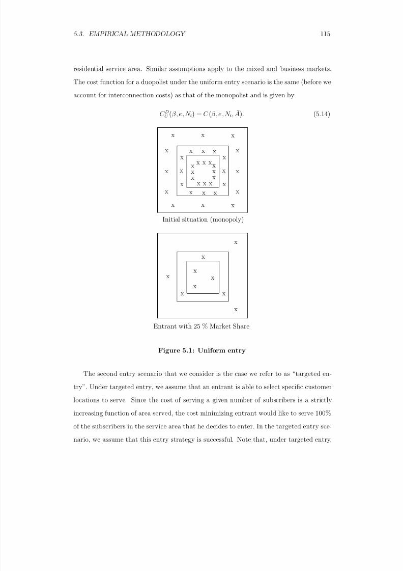
8/18/2019 Gasmi Cost Proxy Models
http://slidepdf.com/reader/full/gasmi-cost-proxy-models 115/318
5.3. EMPIRICAL METHODOLOGY 115
residential service area. Similar assumptions apply to the mixed and business markets.
The cost function for a duopolist under the uniform entry scenario is the same (before weaccount for interconnection costs) as that of the monopolist and is given by
C DU (β, e, N i) = C (β, e, N i, A). (5.14)
x x x
x x x
xxx
xxx
x x xx
x
xx x x
x
x
x
x x x
x x x
x
x
x
x
x
x
Initial situation (monopoly)
x
x
x
x
xx
x
x
x
Entrant with 25 % Market Share
Figure 5.1: Uniform entry
The second entry scenario that we consider is the case we refer to as “targeted en-
try”. Under targeted entry, we assume that an entrant is able to select specific customer
locations to serve. Since the cost of serving a given number of subscribers is a strictly
increasing function of area served, the cost minimizing entrant would like to serve 100%
of the subscribers in the service area that he decides to enter. In the targeted entry sce-
nario, we assume that this entry strategy is successful. Note that, under targeted entry,

8/18/2019 Gasmi Cost Proxy Models
http://slidepdf.com/reader/full/gasmi-cost-proxy-models 116/318
116 CHAPTER 5. THE NATURAL MONOPOLY TEST
subscriber density is the same for each duopolist, and is equal to the subscriber density of
a monopoly provider. Targeted entry is illustrated in Figure 5.2 below. The cost functionfor a duopolist in this scenario is defined by
C DT (β, e, N i) = C (β, e, N i, A × N i/(N 1 + N 2)). (5.15)
x x x
x x x
xxx
xxx
x x xx
x
xx x x
x
x
x
x x x
x x x
x
x
x
x
x
x
Initial situation (monopoly)
Entrant with 25 % Market Share
x x x
x x x
x x x
Figure 5.2: Targeted entry
5.3.3 Interconnection Costs
As indicated above, in our second approach using access lines as output we take into
account the costs of traffic that originates on one network and terminates on a differ-
ent network in the case of duopoly. LECOM was originally conceived for a monopoly

8/18/2019 Gasmi Cost Proxy Models
http://slidepdf.com/reader/full/gasmi-cost-proxy-models 117/318
5.3. EMPIRICAL METHODOLOGY 117
environment. While it includes the cost of providing swiching and interoffice transmis-
sion capacity to handle toll traffic which is carried outside of the local network to a tollprovider’s point of presence (a user input sets the amount of toll traffic as a percentage of
total traffic), there is no comparable method of accounting for the cost of interconnecting
with an alternative local access provider. We believe that it is important to account for
these costs in any analysis that attempts to evaluate the performance of duopoly versus
monopoly.
Consider the case of a duopoly equilibrium in which each firm supplies exactly onehalf of the market. As described above, we are able to estimate the costs of such a
firm in the case of both uniform and targeted entry. Figure 5.3a below illustrates a
stylized representation of a LECOM simulation for a targeted duopolist serving 50% of
the entire market. The relevant costs include the cost of access lines which connect each
subscriber to a local switch, as well as the cost of the switching and interoffice transport
capacity necessary to provide the assumed level of usage demand among all subscribers
in the duopolist’s network. In Figure 5.3b, we illustrate the network that both duopolists
would construct assuming that each duopolist carried only the traffic that both originates
and terminates on its own network. In order to measure the increase in switching and
interoffice transport capacity that would be required to carry inter-network traffic, we
treat the combined network as if it were a monopoly, and run a constrained LECOM
simulation of the resulting costs. That is, we take the exact set of switch locations
and levels of network investment that LECOM calculates for the two duopoly firms in
isolation, and perform a new simulation to compute total network costs assuming that the
monopoly network is constrained to use the duopoly investments. The resulting network
is illustrated in Figure 5.3c.
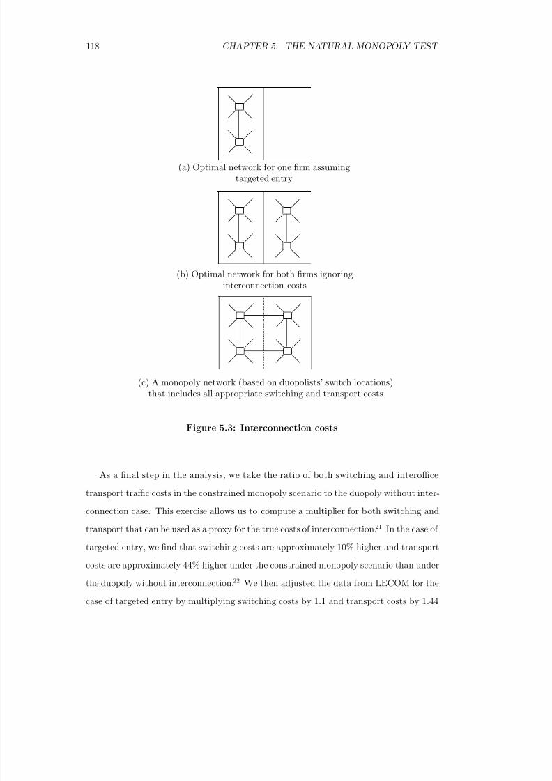
8/18/2019 Gasmi Cost Proxy Models
http://slidepdf.com/reader/full/gasmi-cost-proxy-models 118/318
118 CHAPTER 5. THE NATURAL MONOPOLY TEST
(a) Optimal network for one firm assumingtargeted entry
(b) Optimal network for both firms ignoringinterconnection costs
(c) A monopoly network (based on duopolists’ switch locations)that includes all appropriate switching and transport costs
Figure 5.3: Interconnection costs
As a final step in the analysis, we take the ratio of both switching and interoffice
transport traffic costs in the constrained monopoly scenario to the duopoly without inter-
connection case. This exercise allows us to compute a multiplier for both switching and
transport that can be used as a proxy for the true costs of interconnection.21 In the case of
targeted entry, we find that switching costs are approximately 10% higher and transport
costs are approximately 44% higher under the constrained monopoly scenario than under
the duopoly without interconnection.22 We then adjusted the data from LECOM for the
case of targeted entry by multiplying switching costs by 1.1 and transport costs by 1.44
8/18/2019 Gasmi Cost Proxy Models
http://slidepdf.com/reader/full/gasmi-cost-proxy-models 119/318
5.3. EMPIRICAL METHODOLOGY 119
for each simulation. These data were then used to obtain a translog representation of the
duopoly cost function for that scenario. For the case of uniform entry, a similar exercisefound that switching costs increased by 0.56% and transport costs increased by 5.6% in
comparing the constrained monopoly to the unconstrained duopoly outcomes. We used
these values to adjust the raw LECOM data which then were used to estimate a translog
cost function.23
5.3.4 Calibration of Demand and Disutility
We have described above how, in our two approaches and for each scenario, we have
defined a cost function in terms of three independent variables - technology, effort and
output. The next step is to specify the market demand function and the cost of public
funds in order to obtain some measure of social surplus. Since public funds are obtained
through taxation, their cost depends upon the efficiency of the tax collection system.
In our analysis, we use the value of 0.3 as a benchmark, suggesting that each dollar
transferred to the firm costs 1.3 dollars to society.24 As to the demand function, we have
used an exponential form.25 The two parameters of the exponential demand function
were determined through calibration by relying on two assumptions. First, we assumed
that the elasticity of demand is equal to -0.2 and -0.05 when, respectively, output is
usage and access. Second, we assumed that revenue collected from the representative
customer covers the cost of serving this customer, which by using LECOM amounts to
approximately $240.26 These two assumptions yield two independent equations that we
solve to obtain the (inverse) demand functions we use in the two approaches. When usage
is taken as the output we obtain
P (q ) = −421Log[0.204683q ], (5.16)
whereas, when access is the output, we obtain
P (q ) = −4800Log[0.951229q ]. (5.17)
Clearly, much less is known about the disutility of effort function than about market
8/18/2019 Gasmi Cost Proxy Models
http://slidepdf.com/reader/full/gasmi-cost-proxy-models 120/318
120 CHAPTER 5. THE NATURAL MONOPOLY TEST
demand since the variables that this function is meant to represent are, by definition,
unobservable. Nevertheless, any increasing convex function would be consistent withtheory. We have specified a polynomial form of degree 2 when usage is the output and
of degree 4 when access is the output. In order to calibrate these functions we use the
facts that, under cost-plus regulation, the marginal disutility of effort should be equal to
zero and that after deregulation it should be equal to marginal cost saving. We also make
the assumption that labor force gets reduced by 40% after deregulation.27 This yields
disutility of effort functions of the form
ψ(e) = (1.04397 × 10⁷)e2, (5.18)
and
ψ(e) = (1.20928 × 10⁷)e4, (5.19)
in, respectively, the first (usage as output) and the second (access as output) case. Since
we do not have detailed information about the regulatory environment, we have assumed
a uniform probability distribution to model the regulator’s uncertainty about the technol-
ogy. The support of this distribution has been assumed to be [0.5; 1.5], which includes the
values for which the LECOM cost functions have been defined in our simulations. When
usage is the output, we also examine how sensitive the results of the natural monopoly test
are to the demand elasticity used in the calibration, the distribution of the technological
parameter β and the cost of public funds λ.
5.4 Empirical Results
We have argued above that any criterion that is to be used in a comparison of monopoly
and duopoly should account for the differences in not only technological efficiency but
also consumer and producer surpluses. Aggregate social welfare therefore appears as the
appropriate measure of performance since it encompasses both of those factors. We have
calculated social welfare in each of the market structure scenarios discussed above, which

8/18/2019 Gasmi Cost Proxy Models
http://slidepdf.com/reader/full/gasmi-cost-proxy-models 121/318
5.4. EMPIRICAL RESULTS 121
we summarize in Table 5.1 below. In the following subsections, we analyze the details of
the results in the two cases we consider. Case I is the case where usage is assumed to bethe output and Case II is the case where access is the output.
Table 5.1Market structure scenarios
Scenario DescriptionLT Optimally regulated monopolyPC Price cap regulated monopoly
C+ Cost plus regulated monopolyUM Unregulated monopolyCD Cournot duopolyAC Average cost pricing duopolyMC Marginal cost pricing duopolyYS Yardstick competition duopoly
5.4.1 Case I: Usage as Output
5.4.1.1 Results
Table 5.2 below reports effort e and (total industry) output Q, for different values of the
firm’s type β , under the market structures optimally regulated monopoly (LT ), Yardstick
competition regulated duopoly (Y S ), unregulated Cournot duopoly (CD) and unregu-
lated monopoly (U M ), discussed in Section 5.2 above. Table 5.3 gives social welfare
achieved under these alternative scenarios. A casual look at the data presented in thesetables shows that except for LT , effort is not sensitive to the technological efficiency pa-
rameter β . Output and social welfare are moderately sensitive to β . Figures 5.4, 5.5 and
5.6 illustrate these results.
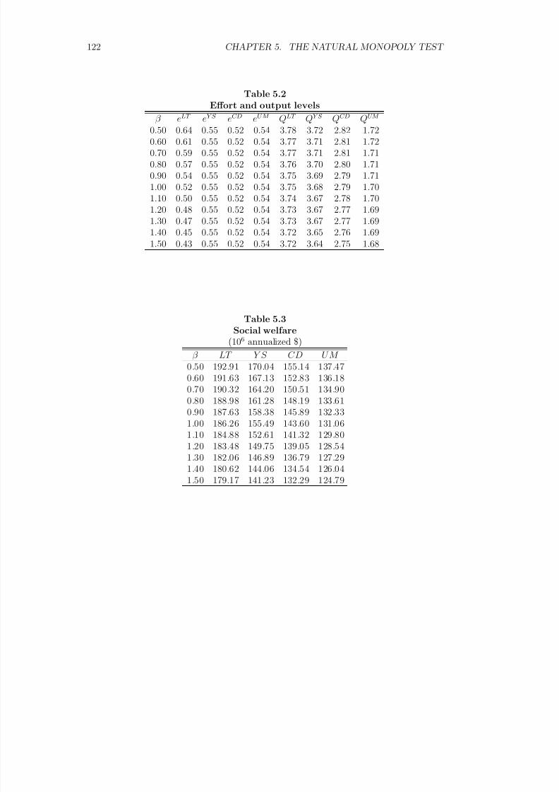
8/18/2019 Gasmi Cost Proxy Models
http://slidepdf.com/reader/full/gasmi-cost-proxy-models 122/318
122 CHAPTER 5. THE NATURAL MONOPOLY TEST
Table 5.2Effort and output levels
β eLT eY S eCD eU M QLT QY S QCD QUM
0.50 0.64 0.55 0.52 0.54 3.78 3.72 2.82 1.720.60 0.61 0.55 0.52 0.54 3.77 3.71 2.81 1.720.70 0.59 0.55 0.52 0.54 3.77 3.71 2.81 1.710.80 0.57 0.55 0.52 0.54 3.76 3.70 2.80 1.710.90 0.54 0.55 0.52 0.54 3.75 3.69 2.79 1.711.00 0.52 0.55 0.52 0.54 3.75 3.68 2.79 1.701.10 0.50 0.55 0.52 0.54 3.74 3.67 2.78 1.701.20 0.48 0.55 0.52 0.54 3.73 3.67 2.77 1.691.30 0.47 0.55 0.52 0.54 3.73 3.67 2.77 1.69
1.40 0.45 0.55 0.52 0.54 3.72 3.65 2.76 1.691.50 0.43 0.55 0.52 0.54 3.72 3.64 2.75 1.68
Table 5.3Social welfare
(106 annualized $)
β LT Y S CD U M 0.50 192.91 170.04 155.14 137.470.60 191.63 167.13 152.83 136.180.70 190.32 164.20 150.51 134.900.80 188.98 161.28 148.19 133.610.90 187.63 158.38 145.89 132.331.00 186.26 155.49 143.60 131.061.10 184.88 152.61 141.32 129.801.20 183.48 149.75 139.05 128.541.30 182.06 146.89 136.79 127.29
1.40 180.62 144.06 134.54 126.041.50 179.17 141.23 132.29 124.79
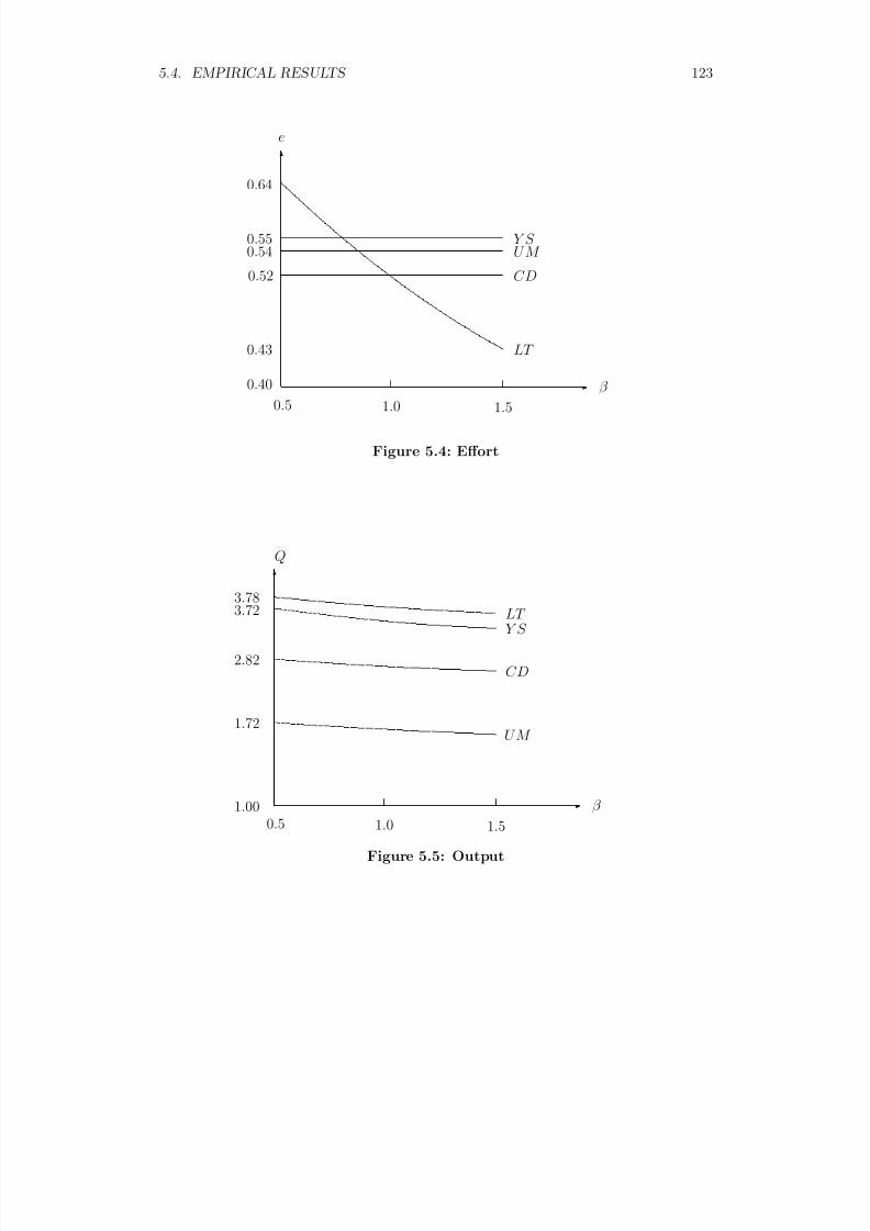
8/18/2019 Gasmi Cost Proxy Models
http://slidepdf.com/reader/full/gasmi-cost-proxy-models 123/318
5.4. EMPIRICAL RESULTS 123
0.52
0.40
0.540.55
0.64
1.5
β
Y S U M
CD
LT
0.5
e
1.0
0.43
Figure 5.4: Effort
1.5
β
0.5
1.0
1.00
1.72
Q
3.783.72
2.82
LT Y S
CD
U M
Figure 5.5: Output
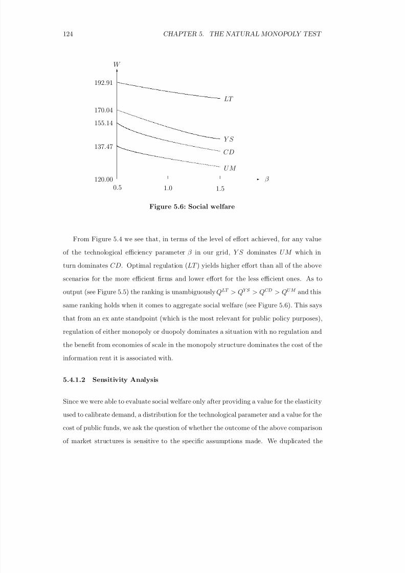
8/18/2019 Gasmi Cost Proxy Models
http://slidepdf.com/reader/full/gasmi-cost-proxy-models 124/318
124 CHAPTER 5. THE NATURAL MONOPOLY TEST
1.5
β
0.5
1.0
W
120.00
192.91
170.04
155.14
137.47
LT
Y S
CD
U M
Figure 5.6: Social welfare
From Figure 5.4 we see that, in terms of the level of effort achieved, for any value
of the technological efficiency parameter β in our grid, Y S dominates UM which in
turn dominates CD. Optimal regulation (LT ) yields higher effort than all of the above
scenarios for the more efficient firms and lower effort for the less efficient ones. As to
output (see Figure 5.5) the ranking is unambiguously QLT > QY S > QCD > QU M and this
same ranking holds when it comes to aggregate social welfare (see Figure 5.6). This says
that from an ex ante standpoint (which is the most relevant for public policy purposes),
regulation of either monopoly or duopoly dominates a situation with no regulation and
the benefit from economies of scale in the monopoly structure dominates the cost of the
information rent it is associated with.
5.4.1.2 Sensitivity Analysis
Since we were able to evaluate social welfare only after providing a value for the elasticity
used to calibrate demand, a distribution for the technological parameter and a value for the
cost of public funds, we ask the question of whether the outcome of the above comparison
of market structures is sensitive to the specific assumptions made. We duplicated the
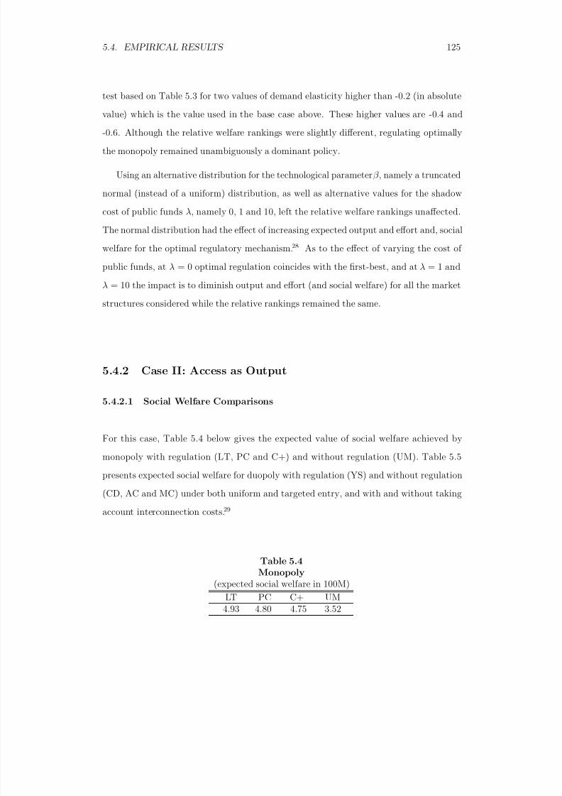
8/18/2019 Gasmi Cost Proxy Models
http://slidepdf.com/reader/full/gasmi-cost-proxy-models 125/318
5.4. EMPIRICAL RESULTS 125
test based on Table 5.3 for two values of demand elasticity higher than -0.2 (in absolute
value) which is the value used in the base case above. These higher values are -0.4 and-0.6. Although the relative welfare rankings were slightly different, regulating optimally
the monopoly remained unambiguously a dominant policy.
Using an alternative distribution for the technological parameter β , namely a truncated
normal (instead of a uniform) distribution, as well as alternative values for the shadow
cost of public funds λ, namely 0, 1 and 10, left the relative welfare rankings unaffected.
The normal distribution had the effect of increasing expected output and effort and, socialwelfare for the optimal regulatory mechanism.28 As to the effect of varying the cost of
public funds, at λ = 0 optimal regulation coincides with the first-best, and at λ = 1 and
λ = 10 the impact is to diminish output and effort (and social welfare) for all the market
structures considered while the relative rankings remained the same.
5.4.2 Case II: Access as Output
5.4.2.1 Social Welfare Comparisons
For this case, Table 5.4 below gives the expected value of social welfare achieved by
monopoly with regulation (LT, PC and C+) and without regulation (UM). Table 5.5
presents expected social welfare for duopoly with regulation (YS) and without regulation
(CD, AC and MC) under both uniform and targeted entry, and with and without taking
account interconnection costs.29
Table 5.4Monopoly
(expected social welfare in 100M)LT PC C+ UM
4.93 4.80 4.75 3.52
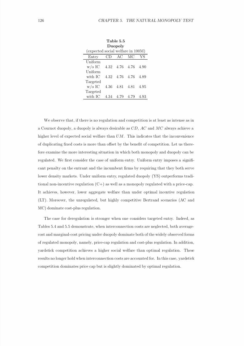
8/18/2019 Gasmi Cost Proxy Models
http://slidepdf.com/reader/full/gasmi-cost-proxy-models 126/318
126 CHAPTER 5. THE NATURAL MONOPOLY TEST
Table 5.5Duopoly
(expected social welfare in 100M)Entry CD AC MC YS
Uniformw/o IC 4.32 4.76 4.76 4.90
Uniformwith IC 4.32 4.76 4.76 4.89
Targetedw/o IC 4.36 4.81 4.81 4.95
Targetedwith IC 4.34 4.79 4.79 4.93
We observe that, if there is no regulation and competition is at least as intense as in
a Cournot duopoly, a duopoly is always desirable as CD, AC and M C always achieve a
higher level of expected social welfare than UM . This indicates that the inconvenience
of duplicating fixed costs is more than offset by the benefit of competition. Let us there-
fore examine the more interesting situation in which both monopoly and duopoly can be
regulated. We first consider the case of uniform entry. Uniform entry imposes a signifi-
cant penalty on the entrant and the incumbent firms by requiring that they both serve
lower density markets. Under uniform entry, regulated duopoly (YS) outperforms tradi-
tional non-incentive regulation (C+) as well as a monopoly regulated with a price-cap.
It achieves, however, lower aggregate welfare than under optimal incentive regulation
(LT). Moreover, the unregulated, but highly competitive Bertrand scenarios (AC and
MC) dominate cost-plus regulation.
The case for deregulation is stronger when one considers targeted entry. Indeed, as
Tables 5.4 and 5.5 demonstrate, when interconnection costs are neglected, both average-
cost and marginal-cost pricing under duopoly dominate both of the widely observed forms
of regulated monopoly, namely, price-cap regulation and cost-plus regulation. In addition,
yardstick competition achieves a higher social welfare than optimal regulation. These
results no longer hold when interconnection costs are accounted for. In this case, yardstick
competition dominates price cap but is slightly dominated by optimal regulation.
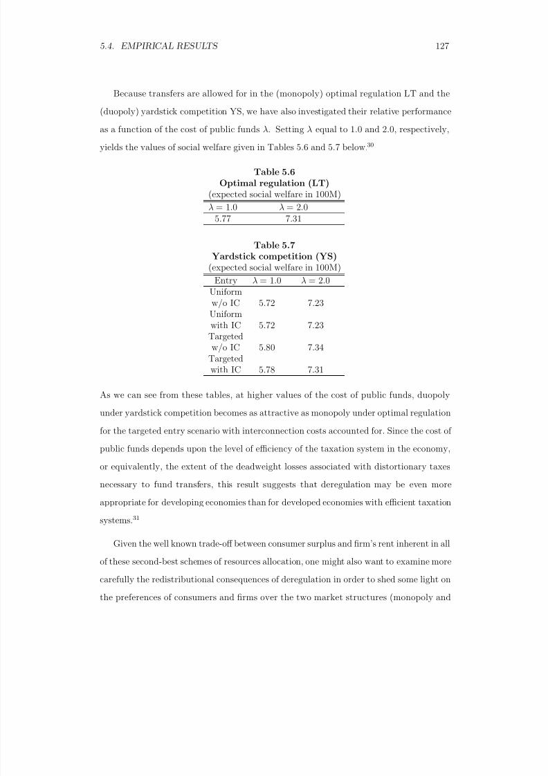
8/18/2019 Gasmi Cost Proxy Models
http://slidepdf.com/reader/full/gasmi-cost-proxy-models 127/318
5.4. EMPIRICAL RESULTS 127
Because transfers are allowed for in the (monopoly) optimal regulation LT and the
(duopoly) yardstick competition YS, we have also investigated their relative performanceas a function of the cost of public funds λ. Setting λ equal to 1.0 and 2.0, respectively,
yields the values of social welfare given in Tables 5.6 and 5.7 below.30
Table 5.6Optimal regulation (LT)
(expected social welfare in 100M)
λ = 1.0 λ = 2.05.77 7.31
Table 5.7Yardstick competition (YS)
(expected social welfare in 100M)
Entry λ = 1.0 λ = 2.0Uniformw/o IC 5.72 7.23
Uniformwith IC 5.72 7.23
Targetedw/o IC 5.80 7.34
Targetedwith IC 5.78 7.31
As we can see from these tables, at higher values of the cost of public funds, duopoly
under yardstick competition becomes as attractive as monopoly under optimal regulation
for the targeted entry scenario with interconnection costs accounted for. Since the cost of
public funds depends upon the level of efficiency of the taxation system in the economy,
or equivalently, the extent of the deadweight losses associated with distortionary taxes
necessary to fund transfers, this result suggests that deregulation may be even more
appropriate for developing economies than for developed economies with efficient taxation
systems.31
Given the well known trade-off between consumer surplus and firm’s rent inherent in all
of these second-best schemes of resources allocation, one might also want to examine more
carefully the redistributional consequences of deregulation in order to shed some light on
the preferences of consumers and firms over the two market structures (monopoly and
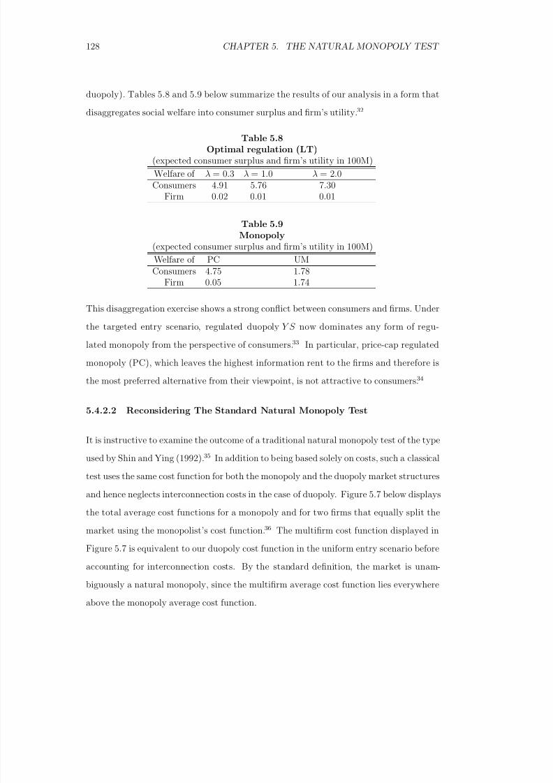
8/18/2019 Gasmi Cost Proxy Models
http://slidepdf.com/reader/full/gasmi-cost-proxy-models 128/318
128 CHAPTER 5. THE NATURAL MONOPOLY TEST
duopoly). Tables 5.8 and 5.9 below summarize the results of our analysis in a form that
disaggregates social welfare into consumer surplus and firm’s utility.32
Table 5.8Optimal regulation (LT)
(expected consumer surplus and firm’s utility in 100M)
Welfare of λ = 0.3 λ = 1.0 λ = 2.0Consumers 4.91 5.76 7.30
Firm 0.02 0.01 0.01
Table 5.9Monopoly
(expected consumer surplus and firm’s utility in 100M)
Welfare of PC UMConsumers 4.75 1.78
Firm 0.05 1.74
This disaggregation exercise shows a strong conflict between consumers and firms. Under
the targeted entry scenario, regulated duopoly Y S now dominates any form of regu-
lated monopoly from the perspective of consumers.33
In particular, price-cap regulated
monopoly (PC), which leaves the highest information rent to the firms and therefore is
the most preferred alternative from their viewpoint, is not attractive to consumers.34
5.4.2.2 Reconsidering The Standard Natural Monopoly Test
It is instructive to examine the outcome of a traditional natural monopoly test of the type
used by Shin and Ying (1992).35
In addition to being based solely on costs, such a classicaltest uses the same cost function for both the monopoly and the duopoly market structures
and hence neglects interconnection costs in the case of duopoly. Figure 5.7 below displays
the total average cost functions for a monopoly and for two firms that equally split the
market using the monopolist’s cost function.36 The multifirm cost function displayed in
Figure 5.7 is equivalent to our duopoly cost function in the uniform entry scenario before
accounting for interconnection costs. By the standard definition, the market is unam-
biguously a natural monopoly, since the multifirm average cost function lies everywhere
above the monopoly average cost function.
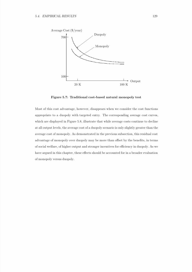
8/18/2019 Gasmi Cost Proxy Models
http://slidepdf.com/reader/full/gasmi-cost-proxy-models 129/318
5.4. EMPIRICAL RESULTS 129
Average Cost ($/year)
Output20 K 100 K
100
700
Monopoly
Duopoly
Figure 5.7: Traditional cost-based natural monopoly test
Most of this cost advantage, however, disappears when we consider the cost functions
appropriate to a duopoly with targeted entry. The corresponding average cost curves,
which are displayed in Figure 5.8, illustrate that while average costs continue to decline
at all output levels, the average cost of a duopoly scenario is only slightly greater than the
average cost of monopoly. As demonstrated in the previous subsection, this residual cost
advantage of monopoly over duopoly may be more than offset by the benefits, in terms
of social welfare, of higher output and stronger incentives for efficiency in duopoly. As we
have argued in this chapter, these effects should be accounted for in a broader evaluation
of monopoly versus duopoly.

8/18/2019 Gasmi Cost Proxy Models
http://slidepdf.com/reader/full/gasmi-cost-proxy-models 130/318
130 CHAPTER 5. THE NATURAL MONOPOLY TEST
Average Cost ($/year)
Output20 K 100 K
100
500
Monopoly
Duopoly
Figure 5.8: Cost-based natural monopoly test - targeted entry
5.5 Conclusion
The evolution of the telecommunications industry throughout the world, beyond any
shadow of doubt, is one of the most interesting recent cases of successful introduction of
technological progress coupled with efforts of countries to implement deregulatory policies.
For example, in the U.S., and to a very large extent elsewhere, since the breakup of the
Bell system in the early eighties, a wave of deregulatory reforms has successively swept
the long distance and the local exchange markets. Even though the trend towards a
generalized deregulation of the industry is a reality which is beyond any dispute, some
observers have come to question the rhythm of arrival of new competitors that has followed
the fall of the regulatory “walls” in the local business and, in some instances, expressed
reservations about its progress.
Given the fast evolution of technology and the questions raised by the new economics
of regulation on the one hand, and the dearth of econometric data, on the other hand,
we have suggested in this chapter an empirical methodology for reconsidering the rel-
ative merits of policies that promote entry into the local exchange market versus the
maintenance of a regulated monopoly. This methodology uses a flexible state-of-the-art
technology process model, along an old tradition pioneered by Frisch (1935), to generate
8/18/2019 Gasmi Cost Proxy Models
http://slidepdf.com/reader/full/gasmi-cost-proxy-models 131/318
5.5. CONCLUSION 131
pseudo data on costs within reasonable ranges of outputs. It then calibrates various mod-
els of monopoly and duopoly markets in order to assess relative performance on the basisof aggregate social welfare. An attractive feature of this methodology is that it allows
us to empirically model incomplete information, a cornerstone of the new economics of
regulation.
The social welfare comparisons of monopoly and duopoly are made under various
assumptions on firms’ behavior, the regulatory context and the nature of the output. In
our first exercise, in which usage is considered as the output and the serving territoryarea and the number of subscribers are held constant, we find a cost elasticity of 0.3
indicating that when output increases by 1% cost increases only by 0.3%. These quite
strong economies of scale allow local exchange telecommunications to retain monopoly
characteristics even when information costs of regulation, due to a cost uncertainty of the
order of 20 to 30% in our case, are properly taken into account. This exercise shows that
even total expropriation of firms’ rents by means of effective yardstick competition is not
enough, in this case, to offset the cost of duplicating fixed costs.
Our second exercise, in which access is considered as the output and average usage is
held constant, develops a richer model of competitive entry, and a broader comparison of
regulated and competitive scenarios. A methodological point made by this latter exercise
is that using a strictly cost-based test of natural monopoly, as is traditionally done, may
be misleading when it comes to evaluating the relative performance of monopoly and
duopoly in a broader sense. Our empirical results strongly demonstrate that deregulatory
policies can enhance social welfare in a variety of situations. The performance of a dereg-
ulated market clearly depends on the assumptions made about the way firms compete.
Under either regulated (YS) competition or highly competitive unregulated competition
(AC or MC) we have found that duopoly outperforms traditional cost plus (C+) reg-
ulated monopoly. In the most favorable targeted entry scenario, yardstick competition
outperforms incentive regulation under price cap regulation (PC), while competitive un-
regulated duopoly achieves slightly lower aggregate social welfare. When only consumer

8/18/2019 Gasmi Cost Proxy Models
http://slidepdf.com/reader/full/gasmi-cost-proxy-models 132/318
132 CHAPTER 5. THE NATURAL MONOPOLY TEST
welfare is used as the criterion, regulated competition is unambiguously preferred to reg-
ulated monopoly, while unregulated competition leads to outcomes which are superior toprice cap regulated monopoly as long as competition is sufficiently intense.
While from the perspective of theory we do not regard the above conclusions as surpris-
ing, we should note that the process model approach, on which our empirical methodology
rests, is the best suited approach for a full exploration of the question of natural monopoly
from a forward-looking point of view. By necessity, the econometric approach must rely
on historical data in which the industry structure and regulatory environment are fixedor rather retrospective. In order to provide a quantitative estimate of the costs and ben-
efits of deregulatory policies in the telecommunications arena, it is necessary to model
as carefully as possible the actual technologies that are most likely to be used by future
entrants and incumbent firms. This chapter is an example of a research approach that can
be used with success in future analyses of telecommunications and other rapidly evolving
industries.
8/18/2019 Gasmi Cost Proxy Models
http://slidepdf.com/reader/full/gasmi-cost-proxy-models 133/318
NOTES 133
Notes
1This is particularly true of labor costs which can have a large variance across regions.
2In this chapter, although we consider the possibility of interfirm rivalry in markets
that might be characterized as natural monopolies, we focus on the final outcome of such
a process, i.e., on the equilibrium state.
3Even more recently, Maher (1999) has estimated a translog cost function in order to
measure access costs at the local level. The data set used by Maher consists of observations
on the central offices of two companies during the year of 1985. The main findings of the
study is that there are differences in access costs across geographical locations but that,
because of significant economies of scale, “... cost-based rates at the local level wouldn’t
be prohibitively high and would not threaten universal service objective.”
4That is to say, in a forward-looking framework, the relationship between the cost and
market structures needs to be taken into account.
5Using a standard oligopoly modeling framework, von Weizscker (1980) shows the
importance of accounting for welfare effects when drawing policy conclusions concerning
barriers to entry. For example, the author shows that, for a given configuration of demand
and cost parameters, social welfare is higher under restricted entry than under free-entry
Cournot equilibrium. In our analysis, we examine Cournot as well as other Bertrand-
type duopoly equilibria and contrast those with some regulated monopoly outcomes. Our
approach incorporates the impact on welfare of both economies of scale and information
rents in the comparisons of monopoly and duopoly.
6See Chapter 4 (Section 3) for a more technical discussion of this trade-off.
7It is assumed that a higher β corresponds to a less efficient technology and that effort
reduces cost at a decreasing rate.
8Under standard assumptions on demand, the social surplus function V is increasing

8/18/2019 Gasmi Cost Proxy Models
http://slidepdf.com/reader/full/gasmi-cost-proxy-models 134/318
134 NOTES
and concave in output.
9See Chapter 4.
10This optimal level of effort, which will be indicated by a “star” hereafter, solves the
equation C e = −ψ(e) that equates marginal cost-saving and marginal disutility. Hence,
this optimal effort can be expressed as e∗(β, q ).
11The main idea behind yardstick competition is that asymmetric information problems
can be alleviated if the principal uses some measure of the relative performance of theeconomic agents. Shleifer (1985) discusses this concept in the context of regulation.
12Note that, strictly speaking, in the case of the MC model one should account for, if
any, the welfare losses associated with the disconnection of some low-income customers
unable to pay for the fixed fee.
13In this approach, we also assume that interconnection costs are negligible and that
total subscribership is independent of market structure and prices for usage.
14A one-dimensional adverse selection parameter makes both the theoretical and em-
pirical analysis considerably more tractable.
15Note that in our interpretation, P L refers to a parameter (effort) that is endogenous
to the decision-making within the firm, whereas P K refers to an exogenous parameter that
describes the technology type of the firm. Both of these interpretations are permissiblesince LECOM is not intented to be an explicit structural model of economic behavior
equilibrium. The function of LECOM is to describe (approximately) the set of cost
minimizing facilities that an efficient firm would choose to deploy given a set of assumed
input values. Whenever a LECOM input value such as P L is a decision variable for the
firm, it is necessary to determine this value as part of the profit maximization problem
for the firm, subject to the competitive and regulatory constraints in which it operates.
This is the approach we have taken in our empirical work. An alternative interpretation
of P L is that it represents the unit price of labor input where the latter is measured in

8/18/2019 Gasmi Cost Proxy Models
http://slidepdf.com/reader/full/gasmi-cost-proxy-models 135/318
NOTES 135
efficiency units. Then, if the nominal (exogenous) price of labor is held constant, changes
in P L are perfectly (inversely) correlated with changes in underlying effort.
16This corresponds to an area of approximately 150 square kilometers with a density
close to 720 subscribers per square kilometer.
17This range of values corresponds to total cost differences (that can be interpreted as
uncertainty on costs) due to adverse selection (modeled through P K ) and moral hazard
(modeled through P L) that could be as large as 23% and 30%, respectively.
18This empirical cost function is presented in the section corresponding to this chap-
ter of Appendix A that can be found at the end of the book. Again, let us note that
interconnection costs are here neglected.
19Assuming that the number of lines per subscriber remains constant our cost function
in this approach is equivalently a function of the number of subscribers.
20In Chapter 8 we study the case in which an entrant specifically targets the lower cost
business district. This form of targeted entry, however, is not considered in the present
analysis.
21LECOM also reports the disaggregated costs of the feeder and distribution networks.
Theory predicts, and our empirical analysis verifies, that the corresponding multipliers
for distribution should be equal to one, and for the feeder network, close to one.
22Total cost increased by about 6%.
23The appendix at the end of the book gives the specific form of the various cost
functions.
24A mean-value estimate of 0.3 for the shadow cost of public funds λ is considered
reasonable for a developed country such as the United States (see Ballard et al., 1985 and
Hausman and Poterba, 1987).

8/18/2019 Gasmi Cost Proxy Models
http://slidepdf.com/reader/full/gasmi-cost-proxy-models 136/318
136 NOTES
25See Taylor (1994) for an extensive survey of the empirical literature on telecommuni-
cations demand.
26For the purpose of the calibration exercise, both of these assumptions seem plausible
for the case of the U.S. local Telecommunications. Initially we also used an elasticity of
-0.2 for access and the qualitative results of the monopoly vs duopoly exercise were the
same (see Gasmi et al, 1999c). Under both of these assumptions we used P K = 1 and
P L = 1.5 and when output is usage we used q = 4CCS and when output is access we
used q = 60, 000 lines.
27In Chapter 6, we give a more detailed description of these two assumptions that we
use to calibrate the disutility of effort functions.
28The issue of the value of information to the regulator certainly deserves a more careful
investigation.
29
Expected social welfare, expected consumer surplus and firm’s rent (see below) aregiven in hundred million dollars (100M).
30The substantial increase in social welfare at higher values of λ is due to the extremely
low elasticity of demand for access to the network (equal to -0.05) that has been assumed
for this simulation. From (5.1) it follows that social welfare can be expressed as W =
S (q )−[C (β, e, q )+ψ(e)]+λ[P (q )q −C (β, e, q )−t]. For low demand elasticities, the second
term in brackets is positive. Hence, under optimal regulation, telephone subscribers may
contribute to general governmental revenues. At higher elasticities, these results would
no longer hold. We explore these issues in more detail in Chapters 6 and 7 where higher
elasticities are more plausible.
31Note, however, that for less developed countries (LDCs) one should include the effect
of possible corruption of the tax system in the comparisons (in Chapter 8, we explore this
issue in the context of the financing of universal service).
32Note that these tables provide only the relevant information. In particular, two pieces

8/18/2019 Gasmi Cost Proxy Models
http://slidepdf.com/reader/full/gasmi-cost-proxy-models 137/318
NOTES 137
of information are implicit in the results and are therefore not presented in these tables.
First, for all of the scenarios that do not allow for transfers (PC, C+, UM, CD, AC andMC), the results are independent of the cost of public funds λ. Second, the whole social
welfare goes to consumers in the scenarios which do not leave any rent to the firm (C+,
AC, MC and YS).
33For λ = 0.3, see Tables 5.5, 5.8 and 5.9. For λ = 1.0 and λ = 2.0, see Tables 5.7, 5.8
and 5.9. Note that under Y S the firm’s rent is nil.
34Note from Tables 5.5 and 5.9 that Bertrand competition (AC ) dominates P C from
the point of view of consumers.
35In the next chapter, we further compare the results of this study with ours.
36These average cost functions are calculated at the average values of the adverse se-
lection and moral hazard parameters for both monopoly and duopoly.

8/18/2019 Gasmi Cost Proxy Models
http://slidepdf.com/reader/full/gasmi-cost-proxy-models 138/318
138 NOTES

8/18/2019 Gasmi Cost Proxy Models
http://slidepdf.com/reader/full/gasmi-cost-proxy-models 139/318
Chapter 6
Optimal Regulation of a Natural
Monopoly
6.1 Introduction
By now, the reader should be familiar with the methodology suggested in this book for
jointly applying engineering and economic models to the empirical analysis of telecommu-
nications markets. The previous chapter has shown how the LECOM engineering model
can be used to generate a cost function that incorporates some elements of incomplete
information that have been emphasized in the new economics of regulation. Further-
more, we have suggested a technique for obtaining an empirical cost function that takes
explicit account of the relationship between the cost function and the market structure
under which firms operate. Using the same methodology, this chapter considers a local
exchange telecommunications industry which possesses the features of a natural monopoly
and investigates in some detail the economic properties and the implementation of the
optimal incentive regulation of a firm that serves the market.
Recall from the previous two chapters, that in models of incentive regulation the solu-
tions typically depend on detailed information about the cost function (both observable
cost and unobservable disutility of effort) and about the form of the regulator’s beliefs
regarding the uncertain technological parameters. Applying these models therefore re-
quires a careful specification of the relevant cost functions and probability distributions.
139
8/18/2019 Gasmi Cost Proxy Models
http://slidepdf.com/reader/full/gasmi-cost-proxy-models 140/318
140 CHAPTER 6. OPTIMAL REGULATION OF A NATURAL MONOPOLY
Schmalensee (1989) presented some simulation results in which cost and disutility of ef-
fort functions are given specific functional forms. His objective was not to model actualcost structures but rather to compare analytically the performance of linear regulatory
mechanisms, which include cost-plus and price-cap regulation as extreme cases, without
attempting to solve for the optimal mechanism. Gasmi et al. (1994) used the Schmalensee
model in order to measure the trade-off between rent extraction and efficiency in various
incentive regulation mechanisms including optimal regulation under asymmetric informa-
tion. These authors did not attempt to evaluate empirically costs or beliefs, but rather
relied on sensitivity analyses for a range of plausible values for these unknown terms.
Wunsch (1994) applied the Laffont-Tirole model to the regulation of European urban
mass transit firms. The central focus of his work was the empirical estimation of the
parameters of the regulator’s beliefs about technological uncertainty, and the calibration
of the firm’s disutility of effort function.
The objective of this chapter is to carry this line of research a step further by incorpo-
rating into the analysis a detailed model of the firm’s cost. Rather than using field data
and econometric techniques to model costs, we will make use of the engineering simulation
model of the costs of local exchange telecommunications networks LECOM, described in
Chapter 2, to generate cost data. In Section 6.2 we recall the optimal regulatory mech-
anism under asymmetric information and the various functions necessary to analyze the
efficiency and welfare properties of this mechanism.1 In Section 6.3 we describe the way
the LECOM model is used to estimate the cost function used in this chapter and discuss
the manner in which we parameterize the various functions entering the expressions that
characterize the optimal regulatory mechanism, namely, the consumer surplus function,
the disutility of effort function and the density function representing regulatory uncer-
tainty. Section 6.4 presents the empirical results related to the endogenous variables of the
mechanism, the implied values of some welfare measures and the outcome of a sensitivity
analysis of the results to some factors used in the calibration.
A couple of implications of these results are discussed in Section 6.5. First, we evaluate

8/18/2019 Gasmi Cost Proxy Models
http://slidepdf.com/reader/full/gasmi-cost-proxy-models 141/318
6.2. THE OPTIMAL REGULATORY MECHANISM: THEORY 141
the extent of the incentive correction, which expresses the divergence of pricing under the
optimal mechanism from optimal pricing under complete information. Second, we askwhether the optimal regulatory mechanism can be implemented through a menu of linear
contracts. We find that the incentive correction term is small in magnitude and that
optimal regulation can be well approximated by a menu of simple linear contracts. Section
6.6 investigates the stability of the optimal regulatory scheme by using an alternative
disutility of effort function to that used above. We summarize our approach and empirical
findings in a concluding section.
6.2 The Optimal Regulatory Mechanism: Theory
We briefly recap in this section the main features of the optimal regulatory mechanism
with ex post cost observability.2 Recall from Chapter 4 that P (q ) denotes the inverse
demand function for a private good produced by a regulated firm, S (q ) represents gross
consumer surplus, and V (q ) = S (q ) + λP (q )q represents the social value associated withproduction of the good, where λ is the shadow cost of public funds.
The firm has private information about (knows) its technological parameter β , which
we refer to as the type of the firm. In addition, the firm exerts an unobservable level of
“effort” e, which reduces costs, according to C = C (β, e, q ) for a production level q , but
which also generates a disutility to the firm of ψ(e) with ψ > 0 and ψ > 0. The utility of
the firm, which chooses effort level e, is given by U = t − ψ(e) where t is the net transferto the firm determined by the regulatory mechanism. The regulator is assumed to have
beliefs about the uncertain technological parameter given by a cumulative distribution
F (β ) on the interval [β, β ] with density f (β ).
Recall that the utilitarian social welfare function (the sum of the consumers’ and firm’s
welfare) is given by
W = V (q ) − (1 + λ)[C (β, e, q ) + ψ(e)] − λU. (6.1)
8/18/2019 Gasmi Cost Proxy Models
http://slidepdf.com/reader/full/gasmi-cost-proxy-models 142/318
142 CHAPTER 6. OPTIMAL REGULATION OF A NATURAL MONOPOLY
The regulator is assumed to have complete information about this objective function,
except for the values of β and e. (That is, the regulator knows the functions P (·), C (·)and ψ(·)).
As seen in Chapter 4, a regulatory mechanism is equivalent to a truthful revela-
tion mechanism {q (β ), C (β ), t(β )}. Cost observation allows the regulator to invert C =
C (β, e, q ) to obtain the effort function E (β, C , q ). The regulatory mechanism can there-
fore be rewritten as {q (β ), e(β ), U (β )} where e(β ) = E (β, C (β ), q (β )) and U (β ) = t(β ) −
ψ(e(β )). The regulatory program is thus given by
maxq(·),e(·),U (·)
β
β
V (q (β )) − (1 + λ) [C (β, e(β ), q (β )) + ψ(e(β ))]
−λU (β )
f (β )dβ, (6.2)
under the participation and incentive compatibility constraints given by
U (β ) ≥ 0 for all β in β, β (6.3)
and
U (β ) = −ψ(e(β ))E β (β, C (β, e(β ), q (β )), q (β )). (6.4)
Integrating (6.4), using (6.3)3 and substituting for U (β ) in (6.2) yields the regulatory
program
maxq(·),e(·)
β
β
V (q (β )) − (1 + λ) [C (β, e(β ), q (β )) + ψ(e(β ))]
+λF (β )
f (β )ψ(e(β ))
C β (β, e(β ), q (β ))
C e(β, e(β ), q (β ))
f (β )dβ. (6.5)
In order to quantify the variables which are endogenous to this optimal regulatory mech-
anism for the case of local exchange telecommunications markets, we proceed to develop
appropriate measures for each of the terms which enter the regulator’s objective function
(6.5).
8/18/2019 Gasmi Cost Proxy Models
http://slidepdf.com/reader/full/gasmi-cost-proxy-models 143/318
6.3. THE LOCAL EXCHANGE COST FUNCTION, WELFARE AND REGULATORY:143
6.3 The Local Exchange Cost Function, Welfare and
Regulatory Uncertainty: Estimation and Cali-bration
In Subsection 3.1 of the previous chapter we have provided a justification of the way we use
some input parameters of the LECOM engineering cost computation software to model
elements of incomplete information that affect the cost function. More specifically, those
LECOM input parameters are used to model an adverse selection parameter representing
some uncertainty that the regulator has on the firm’s production technology and a moral
hazard variable that measures the intensity of the firm’s (unobservable) investment in
a cost-reducing activity. Here, we devote more attention to the procedure we use to
construct this cost function which, as one can see from the previous section, is a critical
component of the optimal regulatory mechanism.
We recall from Chapter 5 that we use the ranges of values [0.5; 1.5] and [0.5; 5.5]
for, respectively, the capital and labor price multipliers (P K and P L) and the level of
telephone usage measured in C CS (output Q) to run LECOM and generate cost data for
a firm covering an area of about 57 square miles and serving 108,000 subscribers. These
data are then used to fit a cost function of the translog form. However, we have to take
care of the two following minor difficulties. First, increasing the level of effort reduces
cost, whereas an increase in the multiplier of the price of labor P L increases cost. Second,
since these data are to be used to fit a translog functional form for the cost function, it is
necessary that the values of all independent variables be bounded away from zero.
Let P L0 = 1.50 be the maximal value of the price of labor in the grid that we consider.
It corresponds to the minimum level of effort equal to an arbitrary small number . Effort
e decreases the price of labor P L according to P L = P L0 + − e, i.e., e = P L0 + − P L.
Then, we can define the empirical cost function C from the theoretical cost function C
according to:
C (PK , PL , Q) = C (P K , P L0 + − PL , Q). (6.6)
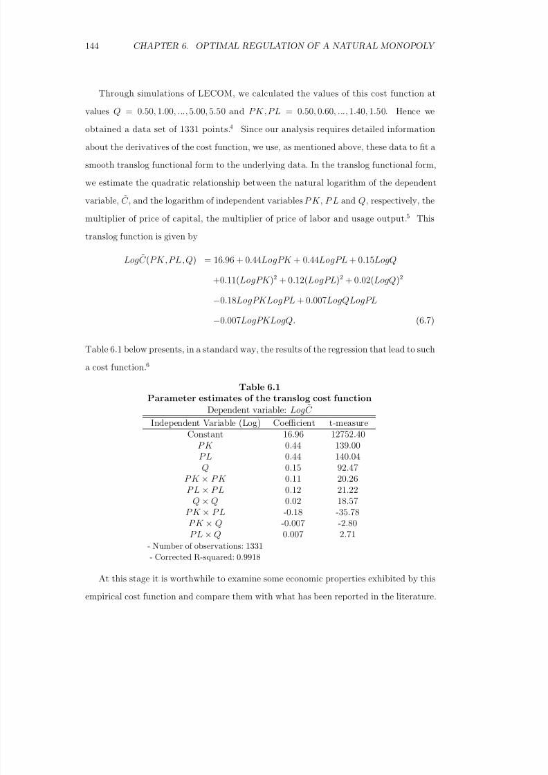
8/18/2019 Gasmi Cost Proxy Models
http://slidepdf.com/reader/full/gasmi-cost-proxy-models 144/318
144 CHAPTER 6. OPTIMAL REGULATION OF A NATURAL MONOPOLY
Through simulations of LECOM, we calculated the values of this cost function at
values Q = 0.50, 1.00, ..., 5.00, 5.50 and P K , P L = 0.50, 0.60, ..., 1.40, 1.50. Hence weobtained a data set of 1331 points.4 Since our analysis requires detailed information
about the derivatives of the cost function, we use, as mentioned above, these data to fit a
smooth translog functional form to the underlying data. In the translog functional form,
we estimate the quadratic relationship between the natural logarithm of the dependent
variable, C , and the logarithm of independent variables P K , P L and Q, respectively, the
multiplier of price of capital, the multiplier of price of labor and usage output. 5 This
translog function is given by
Log C (PK , PL , Q) = 16.96 + 0.44LogPK + 0.44LogPL + 0.15LogQ
+0.11(LogPK )2 + 0.12(LogPL)2 + 0.02(LogQ)2
−0.18LogPKLogPL + 0.007LogQLogPL
−0.007LogPKLogQ. (6.7)
Table 6.1 below presents, in a standard way, the results of the regression that lead to such
a cost function.6
Table 6.1Parameter estimates of the translog cost function
Dependent variable: Log C
Independent Variable (Log) Coefficient t-measureConstant 16.96 12752.40
P K 0.44 139.00
P L 0.44 140.04Q 0.15 92.47
P K × P K 0.11 20.26P L × P L 0.12 21.22
Q × Q 0.02 18.57P K × P L -0.18 -35.78P K × Q -0.007 -2.80P L × Q 0.007 2.71
- Number of observations: 1331
- Corrected R-squared: 0.9918
At this stage it is worthwhile to examine some economic properties exhibited by this
empirical cost function and compare them with what has been reported in the literature.
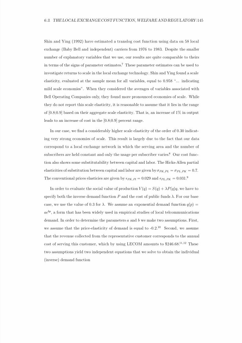
8/18/2019 Gasmi Cost Proxy Models
http://slidepdf.com/reader/full/gasmi-cost-proxy-models 145/318
6.3. THE LOCAL EXCHANGE COST FUNCTION, WELFARE AND REGULATORY:145
Shin and Ying (1992) have estimated a translog cost function using data on 58 local
exchange (Baby Bell and independent) carriers from 1976 to 1983. Despite the smallernumber of explanatory variables that we use, our results are quite comparable to theirs
in terms of the signs of parameter estimates.7 These parameter estimates can be used to
investigate returns to scale in the local exchange technology. Shin and Ying found a scale
elasticity, evaluated at the sample mean for all variables, equal to 0.958 “... indicating
mild scale economies”. When they considered the averages of variables associated with
Bell Operating Companies only, they found more pronounced economies of scale. While
they do not report this scale elasticity, it is reasonable to assume that it lies in the range
of [0.8;0.9] based on their aggregate scale elasticity. That is, an increase of 1% in output
leads to an increase of cost in the [0.8;0.9] percent range.
In our case, we find a considerably higher scale elasticity of the order of 0.30 indicat-
ing very strong economies of scale. This result is largely due to the fact that our data
correspond to a local exchange network in which the serving area and the number of
subscribers are held constant and only the usage per subscriber varies.8 Our cost func-
tion also shows some substitutability between capital and labor. The Hicks-Allen partial
elasticities of substitution between capital and labor are given by σPK,PL = σPL,PK = 0.7.
The conventional prices elasticies are given by PK,Pl = 0.029 and PL,PK = 0.031.9
In order to evaluate the social value of production V (q ) = S (q ) + λP (q )q , we have to
specify both the inverse demand function P and the cost of public funds λ. For our base
case, we use the value of 0.3 for λ. We assume an exponential demand function q ( p) =
aebp, a form that has been widely used in empirical studies of local telcommunications
demand. In order to determine the parameters a and b we make two assumptions. First,
we assume that the price-elasticity of demand is equal to -0.2. 10 Second, we assume
that the revenue collected from the representative customer corresponds to the annual
cost of serving this customer, which by using LECOM amounts to $246.68.11,12 These
two assumptions yield two independent equations that we solve to obtain the individual
(inverse) demand function
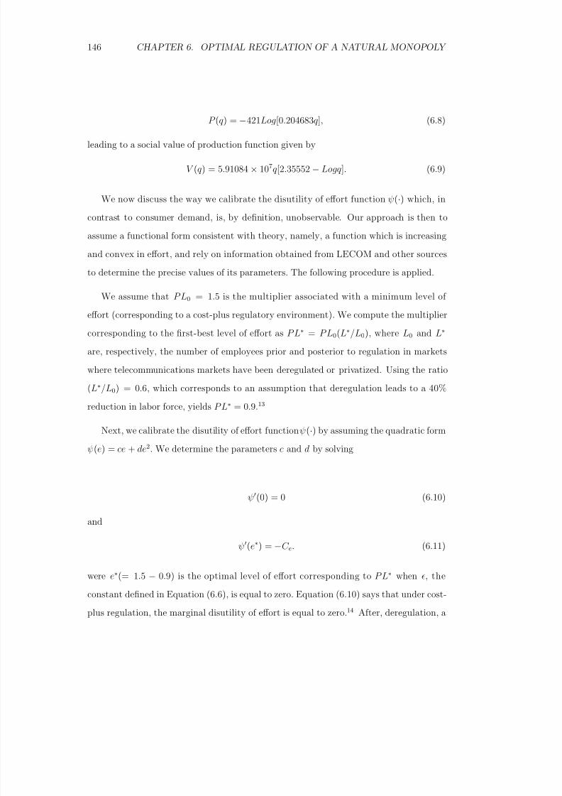
8/18/2019 Gasmi Cost Proxy Models
http://slidepdf.com/reader/full/gasmi-cost-proxy-models 146/318
146 CHAPTER 6. OPTIMAL REGULATION OF A NATURAL MONOPOLY
P (q ) = −421Log[0.204683q ], (6.8)
leading to a social value of production function given by
V (q ) = 5.91084 × 10⁷q [2.35552 − Logq ]. (6.9)
We now discuss the way we calibrate the disutility of effort function ψ(·) which, in
contrast to consumer demand, is, by definition, unobservable. Our approach is then to
assume a functional form consistent with theory, namely, a function which is increasing
and convex in effort, and rely on information obtained from LECOM and other sources
to determine the precise values of its parameters. The following procedure is applied.
We assume that P L0 = 1.5 is the multiplier associated with a minimum level of
effort (corresponding to a cost-plus regulatory environment). We compute the multiplier
corresponding to the first-best level of effort as P L∗ = P L0(L∗/L0), where L0 and L∗
are, respectively, the number of employees prior and posterior to regulation in markets
where telecommunications markets have been deregulated or privatized. Using the ratio
(L∗/L0) = 0.6, which corresponds to an assumption that deregulation leads to a 40%
reduction in labor force, yields P L∗ = 0.9.13
Next, we calibrate the disutility of effort function ψ(·) by assuming the quadratic form
ψ(e) = ce + de2. We determine the parameters c and d by solving
ψ(0) = 0 (6.10)
and
ψ(e∗) = −C e. (6.11)
were e∗(= 1.5 − 0.9) is the optimal level of effort corresponding to P L∗ when , the
constant defined in Equation (6.6), is equal to zero. Equation (6.10) says that under cost-
plus regulation, the marginal disutility of effort is equal to zero. 14 After, deregulation, a

8/18/2019 Gasmi Cost Proxy Models
http://slidepdf.com/reader/full/gasmi-cost-proxy-models 147/318
6.4. THE OPTIMAL REGULATORY MECHANISM: EMPIRICAL EVALUATION 147
cost-minimizing firm sets effort such that marginal disutility equals marginal cost saving
as is shown in Equation (6.11).15
Solving these equations yields parameter values c = 0and d = 1.04397 × 10⁷. The calibrated disutility of effort function is then
ψ(e) = (1.04397 × 10⁷)e2. (6.12)
Finally, concerning the regulatory environment, we assume that the regulator’s un-
certainty about the technological parameter β is captured by a uniform distribution of
this parameter over the range [0.5; 1.5], which is the range of values for which the costfunction has been simulated. We nevertheless examine how sensitive our results are to
changes in the support of this uniform distribution.
6.4 The Optimal Regulatory Mechanism: EmpiricalEvaluation
We now use the empirical cost function given by Equation (6.7), the social valuation of
production given by Equation (6.9) and the uniform distribution with support [0.5;1.5] of
the parameter β to solve the regulator’s program given in (6.5) above. Table 6.2 presents
the optimal levels of output (Q) and effort (e), as a function of firm type (β ).16 We see
that output as well as effort decline as β increases, i.e., as the firm’s efficiency decreases.
It is striking that while effort of the least efficient firm is about 30% lower than that of
the most efficient firm, production drops only by about 2%.
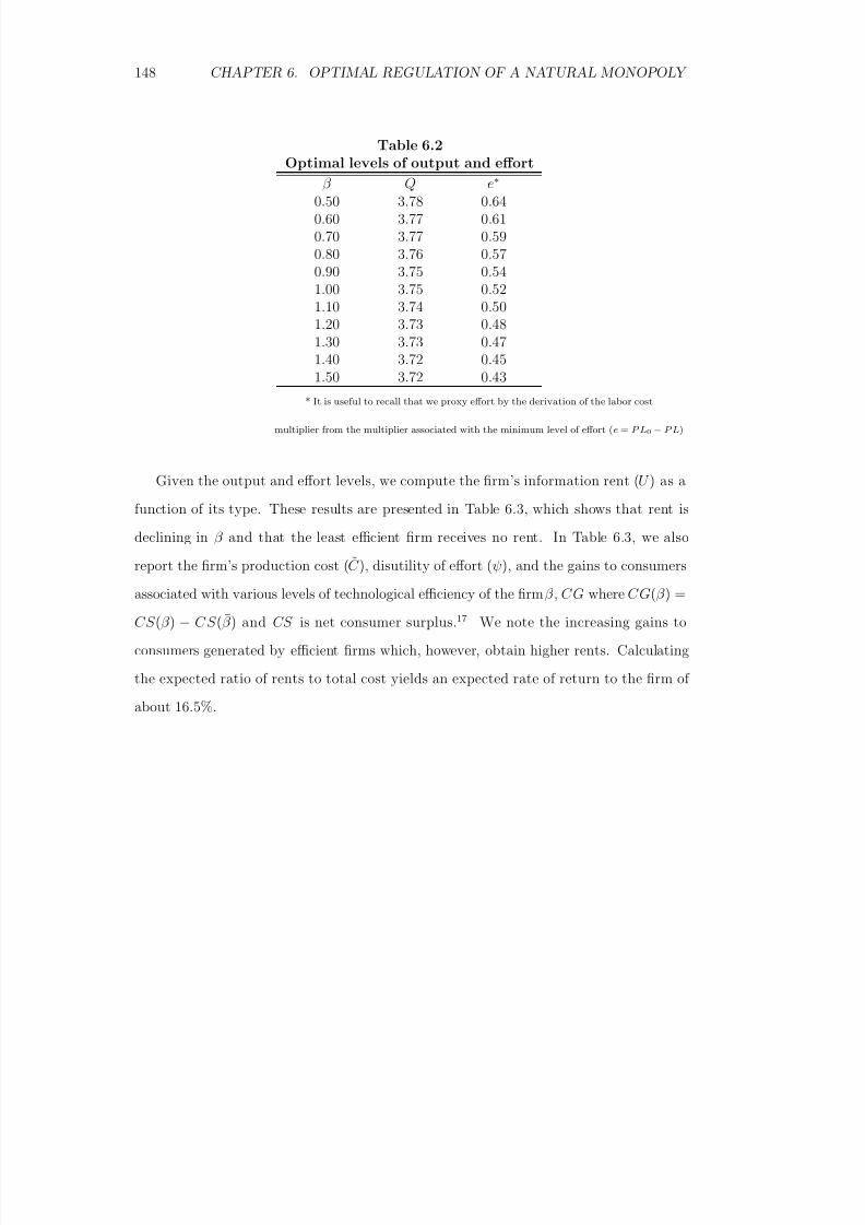
8/18/2019 Gasmi Cost Proxy Models
http://slidepdf.com/reader/full/gasmi-cost-proxy-models 148/318
148 CHAPTER 6. OPTIMAL REGULATION OF A NATURAL MONOPOLY
Table 6.2Optimal levels of output and effort
β Q e∗0.50 3.78 0.640.60 3.77 0.610.70 3.77 0.590.80 3.76 0.570.90 3.75 0.541.00 3.75 0.521.10 3.74 0.501.20 3.73 0.481.30 3.73 0.47
1.40 3.72 0.451.50 3.72 0.43
* It is useful to recall that we proxy effort by the derivation of the labor cost
multiplier from the multiplier associated with the minimum level of effort (e = P L0 − P L)
Given the output and effort levels, we compute the firm’s information rent ( U ) as a
function of its type. These results are presented in Table 6.3, which shows that rent is
declining in β and that the least efficient firm receives no rent. In Table 6.3, we alsoreport the firm’s production cost ( C ), disutility of effort (ψ), and the gains to consumers
associated with various levels of technological efficiency of the firm β , C G where C G(β ) =
CS (β ) − C S (β ) and CS is net consumer surplus.17 We note the increasing gains to
consumers generated by efficient firms which, however, obtain higher rents. Calculating
the expected ratio of rents to total cost yields an expected rate of return to the firm of
about 16.5%.
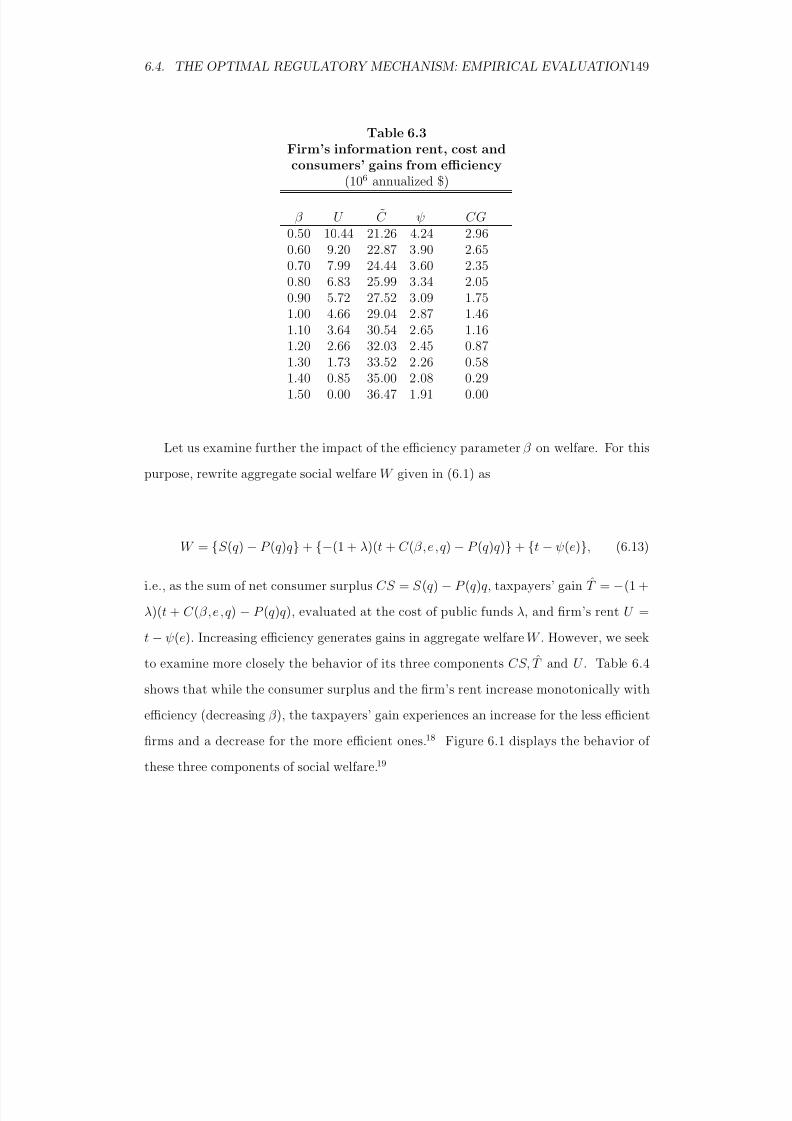
8/18/2019 Gasmi Cost Proxy Models
http://slidepdf.com/reader/full/gasmi-cost-proxy-models 149/318
6.4. THE OPTIMAL REGULATORY MECHANISM: EMPIRICAL EVALUATION 149
Table 6.3Firm’s information rent, cost and
consumers’ gains from efficiency(106 annualized $)
β U C ψ CG0.50 10.44 21.26 4.24 2.960.60 9.20 22.87 3.90 2.650.70 7.99 24.44 3.60 2.350.80 6.83 25.99 3.34 2.050.90 5.72 27.52 3.09 1.751.00 4.66 29.04 2.87 1.46
1.10 3.64 30.54 2.65 1.161.20 2.66 32.03 2.45 0.871.30 1.73 33.52 2.26 0.581.40 0.85 35.00 2.08 0.291.50 0.00 36.47 1.91 0.00
Let us examine further the impact of the efficiency parameter β on welfare. For this
purpose, rewrite aggregate social welfare W given in (6.1) as
W = {S (q ) − P (q )q } + {−(1 + λ)(t + C (β, e, q ) − P (q )q )} + {t − ψ(e)}, (6.13)
i.e., as the sum of net consumer surplus CS = S (q ) − P (q )q , taxpayers’ gain T = −(1 +
λ)(t + C (β, e, q ) − P (q )q ), evaluated at the cost of public funds λ, and firm’s rent U =
t − ψ(e). Increasing efficiency generates gains in aggregate welfare W . However, we seek
to examine more closely the behavior of its three components CS, T and U . Table 6.4
shows that while the consumer surplus and the firm’s rent increase monotonically with
efficiency (decreasing β ), the taxpayers’ gain experiences an increase for the less efficient
firms and a decrease for the more efficient ones.18 Figure 6.1 displays the behavior of
these three components of social welfare.19
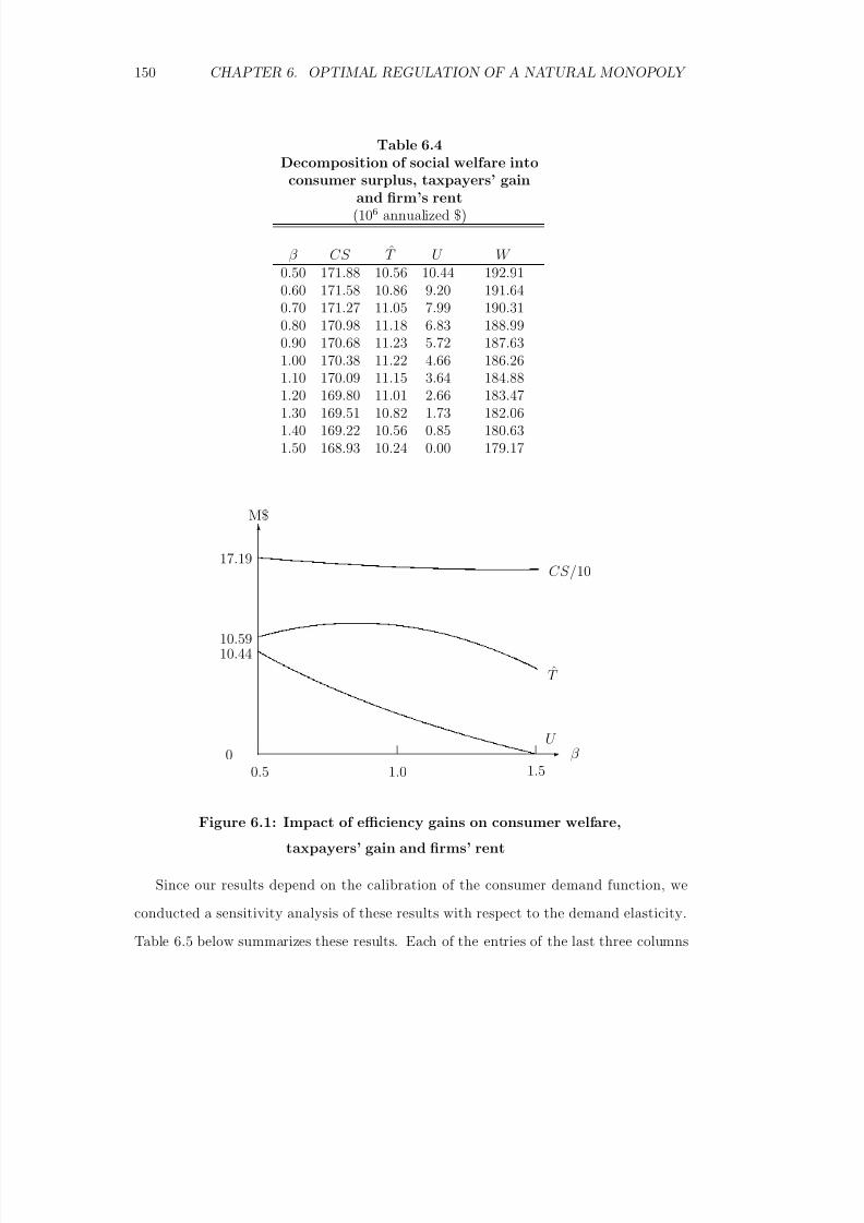
8/18/2019 Gasmi Cost Proxy Models
http://slidepdf.com/reader/full/gasmi-cost-proxy-models 150/318
150 CHAPTER 6. OPTIMAL REGULATION OF A NATURAL MONOPOLY
Table 6.4Decomposition of social welfare into
consumer surplus, taxpayers’ gainand firm’s rent
(106 annualized $)
β CS T U W 0.50 171.88 10.56 10.44 192.910.60 171.58 10.86 9.20 191.640.70 171.27 11.05 7.99 190.310.80 170.98 11.18 6.83 188.990.90 170.68 11.23 5.72 187.63
1.00 170.38 11.22 4.66 186.261.10 170.09 11.15 3.64 184.881.20 169.80 11.01 2.66 183.471.30 169.51 10.82 1.73 182.061.40 169.22 10.56 0.85 180.631.50 168.93 10.24 0.00 179.17
1.50.5 1.0
17.19
10.59
0
10.44
β
M$
CS /10
T
U
Figure 6.1: Impact of efficiency gains on consumer welfare,
taxpayers’ gain and firms’ rent
Since our results depend on the calibration of the consumer demand function, we
conducted a sensitivity analysis of these results with respect to the demand elasticity.
Table 6.5 below summarizes these results. Each of the entries of the last three columns
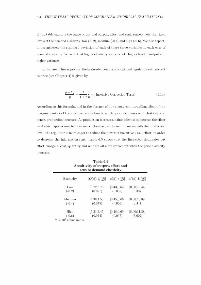
8/18/2019 Gasmi Cost Proxy Models
http://slidepdf.com/reader/full/gasmi-cost-proxy-models 151/318
6.4. THE OPTIMAL REGULATORY MECHANISM: EMPIRICAL EVALUATION 151
of the table exhibits the range of optimal output, effort and rent, respectively, for three
levels of the demand elasticity, low (-0,2), medium (-0.4) and high (-0.6). We also report,in parentheses, the standard deviation of each of these three variables in each case of
demand elasticity. We note that higher elasticity leads to both higher level of output and
higher variance.
In the case of linear pricing, the first-order condition of optimal regulation with respect
to price (see Chapter 4) is given by
p − C q p
= λ
1 + λ
1
η + {Incentive Correction Term}. (6.14)
According to this formula, and in the absence of any strong countervailing effect of the
marginal cost or of the incentive correction term, the price decreases with elasticity and
hence, production increases. As production increases, a first effect is to increase the effort
level which applies now to more units. However, as the rent increases with the production
level, the regulator is more eager to reduce the power of incentives, i.e., effort, in order
to decrease the information rent. Table 6.5 shows that the first-effect dominates but
effort, marginal cost, quantity and rent are all more spread out when the price elasticity
increases.
Table 6.5Sensitivity of output, effort and
rent to demand elasticity
Elasticity [Q(β ); Q(β )] [e(β ); e(β )] [U (β ); U (β )]
Low [3.72;3.78] [0.43;0.64] [0.00;10.44](-0.2) (0.021) (0.065) (3.307)
Medium [4.39;4.53] [0.45;0.66] [0.00;10.89](-0.4) (0.045) (0.066) (3.447)
High [5.21;5.45] [0.48;0.69] [0.00;11.38](-0.6) (0.074) (0.067) (3.602)
* In 106 annualized $.

8/18/2019 Gasmi Cost Proxy Models
http://slidepdf.com/reader/full/gasmi-cost-proxy-models 152/318
152 CHAPTER 6. OPTIMAL REGULATION OF A NATURAL MONOPOLY
We also conducted a sensitivity analysis with respect to the support of the distribution
of the regulator’s prior beliefs about the technological uncertainty parameter β . Whenwe varied the support of the uniform distribution of β , we found that a tighter support,
which can be interpreted as an improvement of information, leads to lower rent for every
firm and higher expected social welfare.20
6.5 Implications
6.5.1 Incentives and Pricing
In our model of incentive regulation described in Section 6.2, asymmetric information
requires the regulator to leave a rent to the firm for inducing efficient production. A
regulator with complete information would set production at a socially efficient level by
equating the marginal social value of production with its social marginal cost,21 that is,
V (q ) = (1 + λ)C q. (6.15)
In addition, a regulator with complete information would ensure that effort is set at its
cost minimizing level, so that
ψ
(e) = −C e. (6.16)
Under asymmetric information, however, the regulator’s desire to minimize the transfer
to the firm is in conflict with his desire to minimize cost. This conflict may give rise to
an incentive distortion as can be seen from the first-order condition of the regulator’s
program (6.5)
V (q ) = (1 + λ)C q + [λF (β )
f (β )ψ(e)
d
dq (∂E/∂β )]. (6.17)
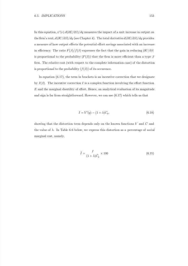
8/18/2019 Gasmi Cost Proxy Models
http://slidepdf.com/reader/full/gasmi-cost-proxy-models 153/318
6.5. IMPLICATIONS 153
In this equation, ψ (e).d(∂E/∂β )/dq measures the impact of a unit increase in output on
the firm’s rent, d(∂U/∂β )/dq (see Chapter 4). The total derivative d(∂E/∂β )/dq providesa measure of how output effects the potential effort savings associated with an increase
in efficiency. The ratio F (β )/f (β ) expresses the fact that the gain in reducing |∂U/∂β |
is proportional to the probability (F (β )) that the firm is more efficient than a type β
firm. The relative cost (with respect to the complete information case) of the distortion
is proportional to the probability (f (β )) of its occurence.
In equation (6.17), the term in brackets is an incentive correction that we designateby I (β ). The incentive correction I is a complex function involving the effort function
E and the marginal disutility of effort. Hence, an analytical evaluation of its magnitude
and sign is far from straightforward. However, we can use (6.17) which tells us that
I = V (q ) − (1 + λ)C q, (6.18)
showing that the distortion term depends only on the known functions V and C and
the value of λ. In Table 6.6 below, we express this distortion as a percentage of social
marginal cost, namely,
I = I
(1 + λ) ˜C q
× 100 (6.19)
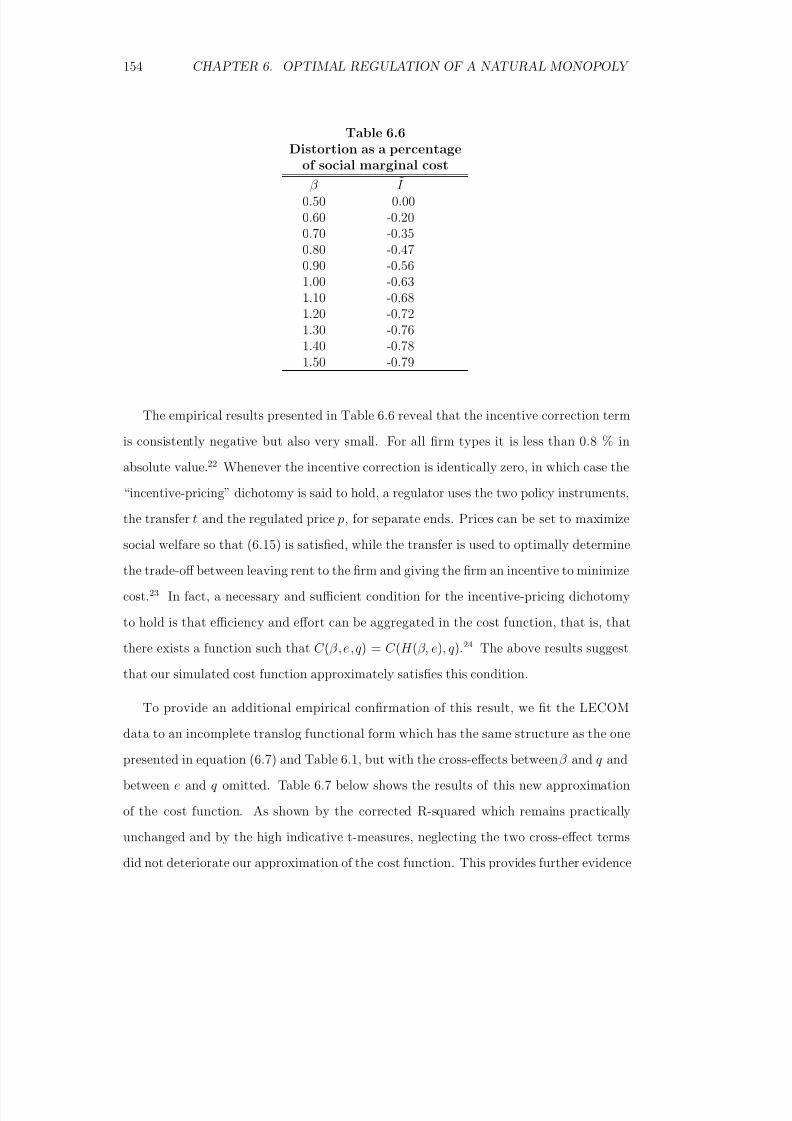
8/18/2019 Gasmi Cost Proxy Models
http://slidepdf.com/reader/full/gasmi-cost-proxy-models 154/318
154 CHAPTER 6. OPTIMAL REGULATION OF A NATURAL MONOPOLY
Table 6.6Distortion as a percentage
of social marginal costβ I
0.50 0.000.60 -0.200.70 -0.350.80 -0.470.90 -0.561.00 -0.631.10 -0.681.20 -0.72
1.30 -0.761.40 -0.781.50 -0.79
The empirical results presented in Table 6.6 reveal that the incentive correction term
is consistently negative but also very small. For all firm types it is less than 0.8 % in
absolute value.22 Whenever the incentive correction is identically zero, in which case the
“incentive-pricing” dichotomy is said to hold, a regulator uses the two policy instruments,
the transfer t and the regulated price p, for separate ends. Prices can be set to maximize
social welfare so that (6.15) is satisfied, while the transfer is used to optimally determine
the trade-off between leaving rent to the firm and giving the firm an incentive to minimize
cost.23 In fact, a necessary and sufficient condition for the incentive-pricing dichotomy
to hold is that efficiency and effort can be aggregated in the cost function, that is, that
there exists a function such that C (β, e, q ) = C (H (β, e), q ).24 The above results suggest
that our simulated cost function approximately satisfies this condition.
To provide an additional empirical confirmation of this result, we fit the LECOM
data to an incomplete translog functional form which has the same structure as the one
presented in equation (6.7) and Table 6.1, but with the cross-effects between β and q and
between e and q omitted. Table 6.7 below shows the results of this new approximation
of the cost function. As shown by the corrected R-squared which remains practically
unchanged and by the high indicative t-measures, neglecting the two cross-effect terms
did not deteriorate our approximation of the cost function. This provides further evidence
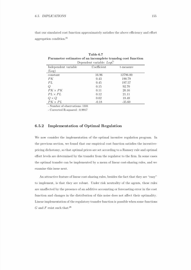
8/18/2019 Gasmi Cost Proxy Models
http://slidepdf.com/reader/full/gasmi-cost-proxy-models 155/318
6.5. IMPLICATIONS 155
that our simulated cost function approximately satisfies the above efficiency and effort
aggregation condition.25
Table 6.7Parameter estimates of an incomplete translog cost function
Dependent variable: Log C
Independent variable Coefficient t-measure(Log)constant 16.96 12796.00
P K 0.43 190.79P L 0.45 197.57Q 0.15 92.70P K × P K 0.11 20.16P L × P L 0.12 21.11Q × Q 0.02 18.48P K × P L -0.18 -35.60- Number of observations: 1331
- Corrected R-squared : 0.9917
6.5.2 Implementation of Optimal Regulation
We now consider the implementation of the optimal incentive regulation program. In
the previous section, we found that our empirical cost function satisfies the incentive-
pricing dichotomy, so that optimal prices are set according to a Ramsey rule and optimal
effort levels are determined by the transfer from the regulator to the firm. In some cases
the optimal transfer can be implemented by a menu of linear cost-sharing rules, and we
examine this issue next.
An attractive feature of linear cost-sharing rules, besides the fact that they are “easy”
to implement, is that they are robust. Under risk neutrality of the agents, these rules
are unaffected by the presence of an additive accounting or forecasting error in the cost
function and changes in the distribution of this noise does not affect their optimality.
Linear implementation of the regulatory transfer function is possible when some functions
G and F exist such that:26
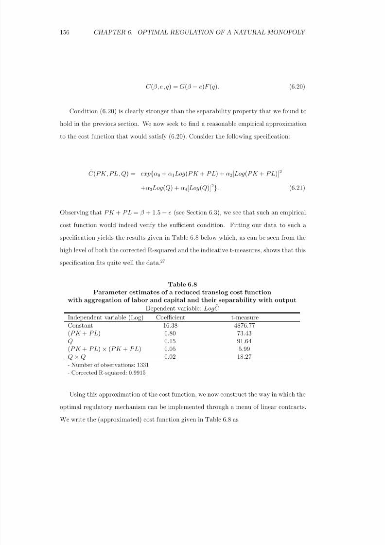
8/18/2019 Gasmi Cost Proxy Models
http://slidepdf.com/reader/full/gasmi-cost-proxy-models 156/318
156 CHAPTER 6. OPTIMAL REGULATION OF A NATURAL MONOPOLY
C (β, e, q ) = G(β − e)F (q ). (6.20)
Condition (6.20) is clearly stronger than the separability property that we found to
hold in the previous section. We now seek to find a reasonable empirical approximation
to the cost function that would satisfy (6.20). Consider the following specification:
C (PK , PL , Q) = exp{α0 + α1Log(P K + P L) + α2[Log(P K + P L)]2
+α3Log(Q) + α4[Log(Q)]2}. (6.21)
Observing that P K + P L = β + 1.5 − e (see Section 6.3), we see that such an empirical
cost function would indeed verify the sufficient condition. Fitting our data to such a
specification yields the results given in Table 6.8 below which, as can be seen from thehigh level of both the corrected R-squared and the indicative t-measures, shows that this
specification fits quite well the data.27
Table 6.8Parameter estimates of a reduced translog cost function
with aggregation of labor and capital and their separability with output
Dependent variable: Log C
Independent variable (Log) Coefficient t-measureConstant 16.38 4876.77(P K + P L) 0.80 73.43Q 0.15 91.64(P K + P L) × (P K + P L) 0.05 5.99Q × Q 0.02 18.27- Number of observations: 1331
- Corrected R-squared: 0.9915
Using this approximation of the cost function, we now construct the way in which the
optimal regulatory mechanism can be implemented through a menu of linear contracts.
We write the (approximated) cost function given in Table 6.8 as
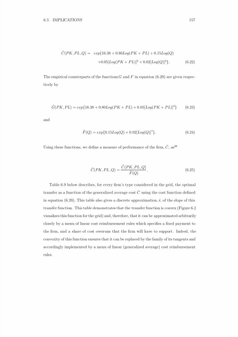
8/18/2019 Gasmi Cost Proxy Models
http://slidepdf.com/reader/full/gasmi-cost-proxy-models 157/318
6.5. IMPLICATIONS 157
C (PK , PL , Q) = exp{16.38 + 0.80Log(P K + P L) + 0.15Log(Q)
+0.05[Log(P K + P L)]2 + 0.02[Log(Q)]2}. (6.22)
The empirical counterparts of the functions G and F in equation (6.20) are given respec-
tively by
G(P K , P L) = exp{16.38 + 0.80Log(P K + P L) + 0.05[Log(P K + P L)]2} (6.23)
and
F (Q) = exp{0.15Log(Q) + 0.02[Log(Q)]2}. (6.24)
Using these functions, we define a measure of performance of the firm, ¯C , as
28
C (PK , PL , Q) =C (PK , PL , Q)
F (Q). (6.25)
Table 6.9 below describes, for every firm’s type considered in the grid, the optimal
transfer as a function of the generalized average cost C using the cost function defined
in equation (6.20). This table also gives a discrete approximation, s, of the slope of this
transfer function. This table demonstrates that the transfer function is convex (Figure 6.2
visualizes this function for the grid) and, therefore, that it can be approximated arbitrarily
closely by a menu of linear cost reimbursement rules which specifies a fixed payment to
the firm, and a share of cost overruns that the firm will have to support. Indeed, the
convexity of this function ensures that it can be replaced by the family of its tangents and
accordingly implemented by a menu of linear (generalized average) cost reimbursementrules.

8/18/2019 Gasmi Cost Proxy Models
http://slidepdf.com/reader/full/gasmi-cost-proxy-models 158/318
158 CHAPTER 6. OPTIMAL REGULATION OF A NATURAL MONOPOLY
Table 6.9Performance ( C ), transfer (t) and slope (s)
of the transfer function
β C t s(106 annualized $) (106 annualized $)
0.50 16.75 14.68 -1.240.60 18.05 13.09 -1.200.70 19.32 11.59 -1.160.80 20.56 10.17 -1.120.90 21.80 8.82 -1.071.00 23.02 7.52 -1.03
1.10 24.25 6.29 -0.981.20 25.46 5.12 -0.941.30 26.68 3.99 -0.901.40 27.90 2.92 -0.861.50 29.11 1.91 -0.82
30161
15
C
t
Figure 6.2: Transfer function
It has been argued in the literature (Wilson, 1989) that, in practice, a few elements
are needed in the menu of linear reimbursement rules for approximating quite closely
the optimal regulation mechanism.29 Below we consider a menu with three elements
and compute the associated welfare loss. We consider the tangents associated with the
transfer-perfomance pairs30 denoted A, B,D in Figure 6.3.
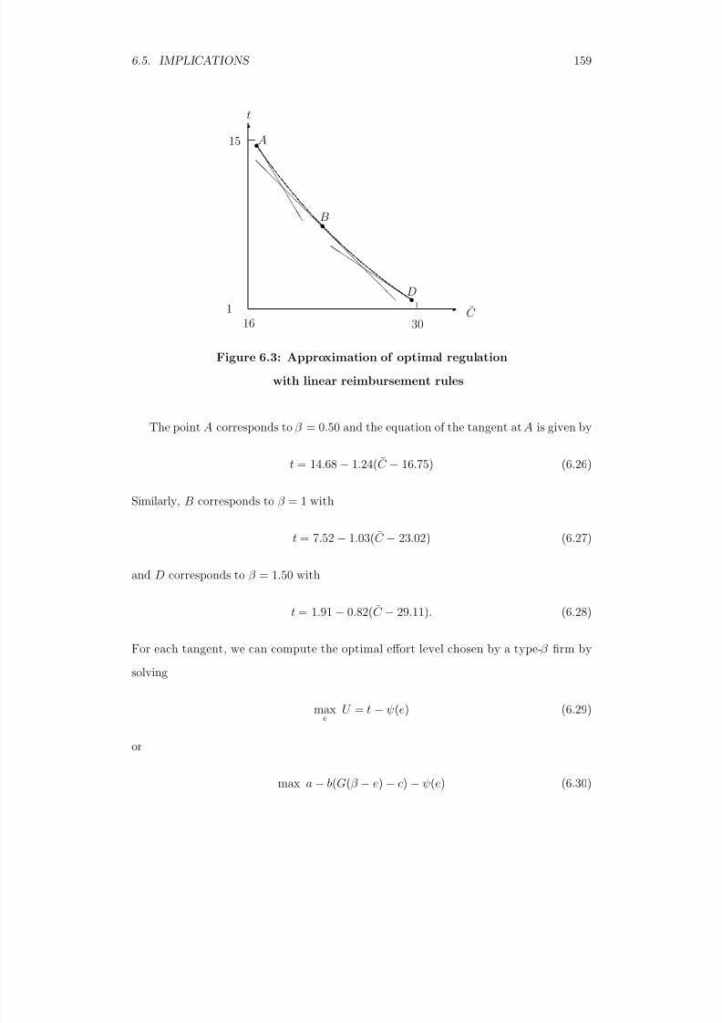
8/18/2019 Gasmi Cost Proxy Models
http://slidepdf.com/reader/full/gasmi-cost-proxy-models 159/318
6.5. IMPLICATIONS 159
30161
15
C
t
A
B
D
Figure 6.3: Approximation of optimal regulation
with linear reimbursement rules
The point A corresponds to β = 0.50 and the equation of the tangent at A is given by
t = 14.68 − 1.24( C − 16.75) (6.26)
Similarly, B corresponds to β = 1 with
t = 7.52 − 1.03( C − 23.02) (6.27)
and D corresponds to β = 1.50 with
t = 1.91 − 0.82( C − 29.11). (6.28)
For each tangent, we can compute the optimal effort level chosen by a type-β firm by
solving
maxe
U = t − ψ(e) (6.29)
or
max a − b(G(β − e) − c) − ψ(e) (6.30)

8/18/2019 Gasmi Cost Proxy Models
http://slidepdf.com/reader/full/gasmi-cost-proxy-models 160/318
160 CHAPTER 6. OPTIMAL REGULATION OF A NATURAL MONOPOLY
where a,b,c are the parameters of the appropriate tangent, G(β − e) is the estimated
function31
G(β − e) = exp{16.38 + 0.80Log(1.5 + β − e) + 0.05[Log(1.5 + β − e)]2} (6.31)
and ψ(e) is the calibrated function
ψ(e) = (1.04395 × 10⁷)e2. (6.32)
We obtain in this way three effort functions eA(β ), eB(β ), eD(β ).
Next, we determine the cut-off points β 1 and β 2 such that
- For β ∈ [β 1, β 1], type β prefers the tangent to A than the tangent to B or D.
- For β ∈ [β 1, β 2], type β prefers the tangent to B than the tangent to A or D.
- For β ∈ [β 2, β ], type β prefers the tangent to D than the tangent to A or B .
The associated information rents are32
U (β ) = β
β
ψ(e∗D(b))db for β ∈ [β 2, β ]
=
β 2
β
ψ(e∗B(b))db +
β
β 2
ψ(e∗D(b))db for β ∈ [β 1, β 2]
=
β 1
β
ψ(e∗A(b))db +
β 2
β 1
ψ(e∗B(b))db +
β
β 2
ψ(e∗D(b))db for β ∈ [β, β 1]
(6.33)
We can then compute the associated best welfare for the regulation by solving
maxq(·)
β
β
[V (q (β )) − (1 + λ)(C (β, e(β ), q (β ) + ψ(e(β ))) − λU (β )]f (β )dβ (6.34)
with
e(β ) = eA(β ) for β ∈ [β, β 1]
= eB(β ) for β ∈ [β 1, β 2]
= eD(β ) for β ∈ [β 2, β ], (6.35)
and compare it with the optimal social welfare. We obtain a loss of 0.054 %.33
8/18/2019 Gasmi Cost Proxy Models
http://slidepdf.com/reader/full/gasmi-cost-proxy-models 161/318
6.6. USING AN ALTERNATIVE DISUTILITY OF EFFORT FUNCTION 161
6.6 Using an Alternative Disutility of Effort Function
This and the other empirical chapters of the book are based on a theoretical framework
in which effort is viewed as the investment that the firm’s manager makes in order to
reduce costs. An assumption appended to this interpretation is that the firm’s disutility
of effort has the nature of a fixed cost, namely, that it is independent of the level of
output. However, if effort is of a more disaggregated nature, e.g., if it affects cost at the
level of each piece of capital, then it is reasonable to assume that the disutility it creates
depends on the level of output. In this section, we present the results of a computation of
the optimal regulatory mechanism using a disutility of effort of the form ψ(e, q ) = ϕ(e)q .
The first-order conditions that define the optimal regulatory mechanism in the general
case ψ(e, q ) have been derived in Chapter 4 (Section 4.7). In the special case where
ψ(e, q ) = ϕ(e)q , the regulatory program that we solve takes the following compact form:
maxq(·),e(·)
β
β
V (q (β )) − (1 + λ)[C (β, e(β ), q (β )) + ϕ(e(β ))q (β )]
+λF (β )
f (β )ϕ(e(β ))q (β )
C β (β, e(β ), q (β ))
C e(β, e(β ), q (β ))
f (β )dβ (6.36)
Using the same calibration techniques as in the case ψ(e), we have solved the program
(6.36). Tables 6.10, 6.11 and 6.12 duplicate Tables 6.2, 6.3 and 6.4 for this case where
ψ(e, q ) = ϕ(e)q . We also have evaluated the incentive distortion as a percentage of social
marginal cost (see Section 6.5.1) and found it to be on average close to 81%. This confirms
our expectation that the incentive-pricing dichotomy does not hold. Besides this expected
result, these new figures show that the main qualitative features of the optimal regulatory
mechanism are robust to this change in the disutility technology.
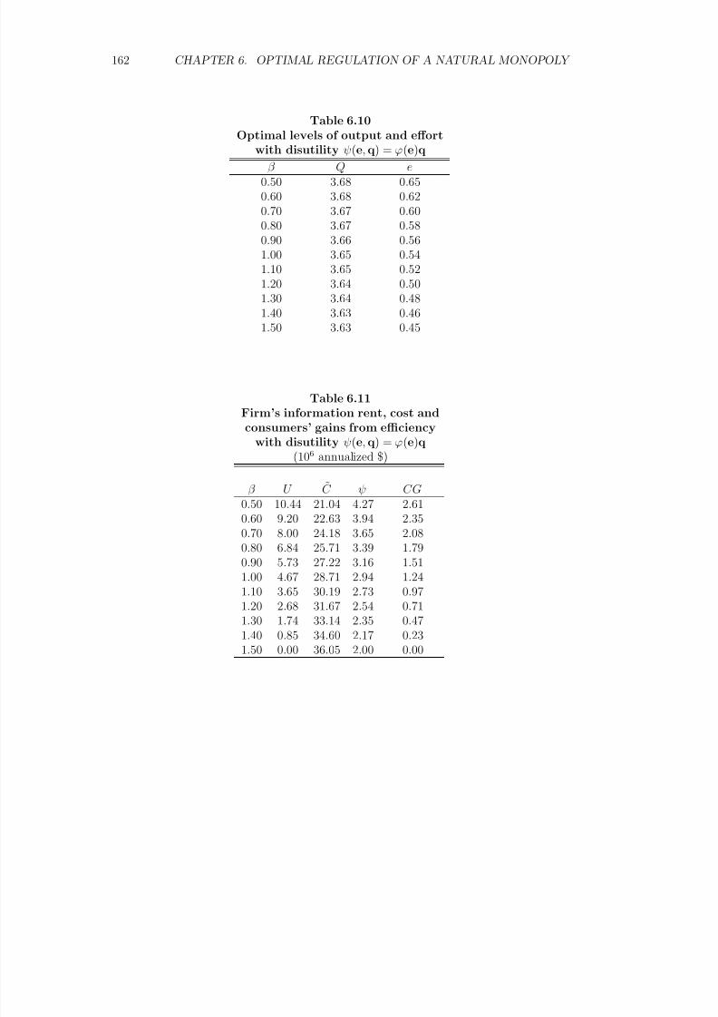
8/18/2019 Gasmi Cost Proxy Models
http://slidepdf.com/reader/full/gasmi-cost-proxy-models 162/318
162 CHAPTER 6. OPTIMAL REGULATION OF A NATURAL MONOPOLY
Table 6.10Optimal levels of output and effort
with disutility ψ(e, q) = ϕ(e)qβ Q e
0.50 3.68 0.650.60 3.68 0.620.70 3.67 0.600.80 3.67 0.580.90 3.66 0.561.00 3.65 0.541.10 3.65 0.521.20 3.64 0.50
1.30 3.64 0.481.40 3.63 0.461.50 3.63 0.45
Table 6.11Firm’s information rent, cost andconsumers’ gains from efficiency
with disutility ψ(e, q) = ϕ(e)q(106 annualized $)
β U C ψ CG0.50 10.44 21.04 4.27 2.610.60 9.20 22.63 3.94 2.350.70 8.00 24.18 3.65 2.080.80 6.84 25.71 3.39 1.790.90 5.73 27.22 3.16 1.511.00 4.67 28.71 2.94 1.241.10 3.65 30.19 2.73 0.971.20 2.68 31.67 2.54 0.711.30 1.74 33.14 2.35 0.471.40 0.85 34.60 2.17 0.231.50 0.00 36.05 2.00 0.00
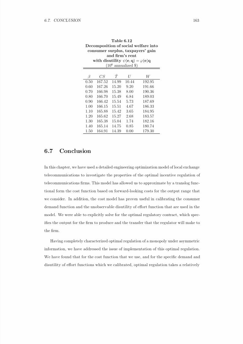
8/18/2019 Gasmi Cost Proxy Models
http://slidepdf.com/reader/full/gasmi-cost-proxy-models 163/318
6.7. CONCLUSION 163
Table 6.12Decomposition of social welfare into
consumer surplus, taxpayers’ gainand firm’s rent
with disutility ψ(e, q) = ϕ(e)q(106 annualized $)
β CS T U W 0.50 167.52 14.99 10.44 192.950.60 167.26 15.20 9.20 191.660.70 166.98 15.38 8.00 190.360.80 166.70 15.49 6.84 189.03
0.90 166.42 15.54 5.73 187.691.00 166.15 15.51 4.67 186.331.10 165.88 15.42 3.65 184.951.20 165.62 15.27 2.68 183.571.30 165.38 15.04 1.74 182.161.40 165.14 14.75 0.85 180.741.50 164.91 14.39 0.00 179.30
6.7 Conclusion
In this chapter, we have used a detailed engineering optimization model of local exchange
telecommunications to investigate the properties of the optimal incentive regulation of
telecommunications firms. This model has allowed us to approximate by a translog func-
tional form the cost function based on forward-looking costs for the output range that
we consider. In addition, the cost model has proven useful in calibrating the consumer
demand function and the unobservable disutility of effort function that are used in the
model. We were able to explicitly solve for the optimal regulatory contract, which spec-
ifies the output for the firm to produce and the transfer that the regulator will make to
the firm.
Having completely characterized optimal regulation of a monopoly under asymmetric
information, we have addressed the issue of implementation of this optimal regulation.
We have found that for the cost function that we use, and for the specific demand and
disutility of effort functions which we calibrated, optimal regulation takes a relatively
8/18/2019 Gasmi Cost Proxy Models
http://slidepdf.com/reader/full/gasmi-cost-proxy-models 164/318
164 CHAPTER 6. OPTIMAL REGULATION OF A NATURAL MONOPOLY
simple form. Prices should be set according to the Ramsey rule, and a monetary transfer
to the firm determines the optimal level of rent to leave to the firm (and simultaneouslythe optimal deviation from cost minimizing behavior for the firm). Moreover, the optimal
transfer can be implemented by a menu of contracts linear in performance and we have
illustrated the design of such contracts.
8/18/2019 Gasmi Cost Proxy Models
http://slidepdf.com/reader/full/gasmi-cost-proxy-models 165/318
NOTES 165
Notes
1To the risk of repeating ourselves, because this chapter focuses on the optimal regu-
latory mechanism, it is worthwhile recalling its main theoretical ingredients.
2See Chapter 4 for more details.
3Appropriate assumptions ensure that ∂E/∂β > 0 so that U (β ) is decreasing in β .
The participation constraint reduces to U (β ) ≥ 0 and from the objective function it is
clear that at the optimum this constraint is binding.
4A LECOM run takes roughly a minute for a medium-sized city of the type we consider
here. A typical simulation with about 600 runs would then approximately take 10 hours
on a machine ranging from 200 MHz to 500 MHz.
5Note that the translog function is viewed as a second-order Taylor expansion (in
natural logarithms) that approximates the true underlying cost function. Given that we
generate our data through a process which may be thought as a deterministic process
(LECOM), the disturbance term in the regression might be thought as merely reflecting
the imprecision of this quadratic approximation fit and not some unobservable random
effect.
6An important point is worth mentioning here though. While the only requirements in
order to properly run the standard OLS method on these cost data are the usual Gauss-
Markov assumptions, the use of the t-statistic to test the significance of the coefficients
necessitates, in the case of small samples, by construction of the student distribution,
the normality of the disturbance term. However, because of the large size of our data
sample, we benefit from the asymptotic normality of the t-statistic. Nevertheless, given
the deterministic nature of our data-generating process (LECOM), the numbers presented
in the third column of Tables 6.1, 6.7 and 6.8 below should only be taken as an “indication”
of the goodness of the respective nul hypotheses. They will be referred to as “t-measures”.
7Also, Shin and Ying report an (uncorrected) R-squared of 0.9977 for their cost equa-
8/18/2019 Gasmi Cost Proxy Models
http://slidepdf.com/reader/full/gasmi-cost-proxy-models 166/318
166 NOTES
tion.
8In contrast, Shin and Ying estimate a cost function using data on firms that serve
areas of different sizes and with different population densities and compute an overall
scale elasticity by summing up their three output (access, local calls and toll calls) cost
elasticities.
9In our context, these elasticities are given by
σPK,PL(PK , PL , Q) = σPL,PK (PK , PL , Q) =
C (PK , PL , Q).C P K P L
C P K .C P L,
PK,PL(PK , PL , Q) = C P K .( P L
C (PK , PL , Q)) and
PL,PK (PK , PL , Q) = C P L.( P K
C (PK , PL , Q)).
10Taylor (1994) reports a demand elasticity in the range [−0.38; −0.17]. In our base
case the value of -0.2 is used at an output q = 4CCS .
11See Section 5.3.4 for some more quantitative details on this demand calibration exer-
cise.
12Two comments are worth making. First, while LECOM can handle disaggregated
output in business, residential, private line, etc., taking a multi-dimensional output ap-
proach would make both the theoretical exposition and the computational burden much
heavier. Relying on an assumption of existence of a representative customer allows us to
circumvent these issues. Second, we assume that the cost of local exchange services must
be fully recovered from local revenues. While telephone rate structures have traditionally
embodied a subsidy from toll to local usage, we believe that, given changing technologies
and liberalized regulatory regimes, this assumption is appropriate for future regulation of
local exchange companies.
13As informal evidence in support of this assumption, see the Wall Street Journal, Oct.
2, 1995, page A6, where the following statement appears: “BT [British Telecom]... like

8/18/2019 Gasmi Cost Proxy Models
http://slidepdf.com/reader/full/gasmi-cost-proxy-models 167/318
NOTES 167
many phone companies around the world, has been forced to gird for the new competition
by slashing costs. Since 1984, when the former state phone monopoly was privatized, BThas shed nearly 102000 jobs, or 43% of its work force.”
14Note that if there is monitoring of effort, then under cost-plus regulation the marginal
disutility of effort is positive but there is a positive cost of monitoring.
15We evaluate the derivative of C with respect to e at average output (3 CCS ) and
average value of the technological parameter β (1).
16These calculations were carried out using Mathematica . Stricly speaking, our cost
function C defined in equation (6.6) is valid only for positive values of . We report in
Table 6.2 the limiting values for e as → 0. We have also directly estimated a translog cost
function C (P K , P L0 + − PL , Q) for positive values of , and for = 0 (by eliminating
data points where necessary). In all cases the regression results were qualitatively the
same as those that we report.
17Recall from Chapter 4 that the net consumer surplus CS (q ) is defined as the gross
consumer surplus S (q ) =
q
0
P (s)ds minus the total consumer expense (the firm’s rev-
enue) R(q ) = P (q )q .
18Note that the non-monotonicity of T does not prevent W from behaving as its two
other components CS and U , i.e., monotonically increasing in efficiency.
19Note that CS is rescalled by dividing by 10.
20See Appendix A2. We also present in the appendix data showing that using the
normal instead of the uniform distribution decreases rents and increases social welfare.
Note, however, that in this model of optimal regulation under asymmetric information an
improvement of the information structure even in the strong sense of Blackwell (1951) is
not necessarily beneficial to the principal (the regulator) because it also affects directly
the information rents.

8/18/2019 Gasmi Cost Proxy Models
http://slidepdf.com/reader/full/gasmi-cost-proxy-models 168/318
168 NOTES
21The complete information regulatory scheme is found by solving
maxq,e
V (q ) − (1 + λ)[C (β, e, q ) + ψ(e)]
22Note from (6.17) that the incentive correction term is nil for the most efficient firm.
23When the incentive-pricing dichotomy holds, the first-order condition of the regula-
tor’s program (6.5) yields the Ramsey formula
p − C q p
= λ1 + λ
. 1η
where η is the demand elasticity (see Chapter 4).
24See Laffont & Tirole (1993) p.179.
25Note, from Table 6.1, that the cross-terms that have been removed are relatively small
in magnitude and have the smallest values of the indicative t-measures.
26This sufficient condition for linear implementation is given in Laffont & Tirole (1993),
p. 171.
27We also have fitted a specification similar to (6.21) which contains the cross-term
Log(P K + P L) × Log(Q) and found that the coefficient corresponding to this term had
a very low t-measure.
28This measure might be thought of as a generalized average cost.
29Proposition 3 in Wilson (1989) shows that priority service which is a form of optimal
non-linear pricing with n priority classes incurs an efficiency less that is of order no more
than 1/n2.
30Ideally, one could optimize over this choice pairs.
31To be more explicit, G(x) = G(0, x) = G(x, 0) where G is given in (6.23) above.
32See Equation (6.4) above. Note that given the form of our cost function E β = 1.
33On the basis of a grid of demand and cost parameters defined by Schmalensee (1989),
8/18/2019 Gasmi Cost Proxy Models
http://slidepdf.com/reader/full/gasmi-cost-proxy-models 169/318
NOTES 169
Gasmi et al. (1997) find values that show a much higher welfare loss of linear regulation
relative to optimal regulation of about 0.5 %. Although using a higher demand elasticitythe welfare loss increased by a factor of 4, the comparison of these results should only be
done at a methodological level for at least two reasons. First, while the exercise of these
authors is based on a grid of parameters which is built mainly for illustration purposes,
ours uses cost data based on real local exchange technology as described by LECOM.
Second, our results still depend on our calibration of the unobservable disutility of effort
function and how sensitive they are to the precise form of this function is still under
investigation.

8/18/2019 Gasmi Cost Proxy Models
http://slidepdf.com/reader/full/gasmi-cost-proxy-models 170/318
170 NOTES
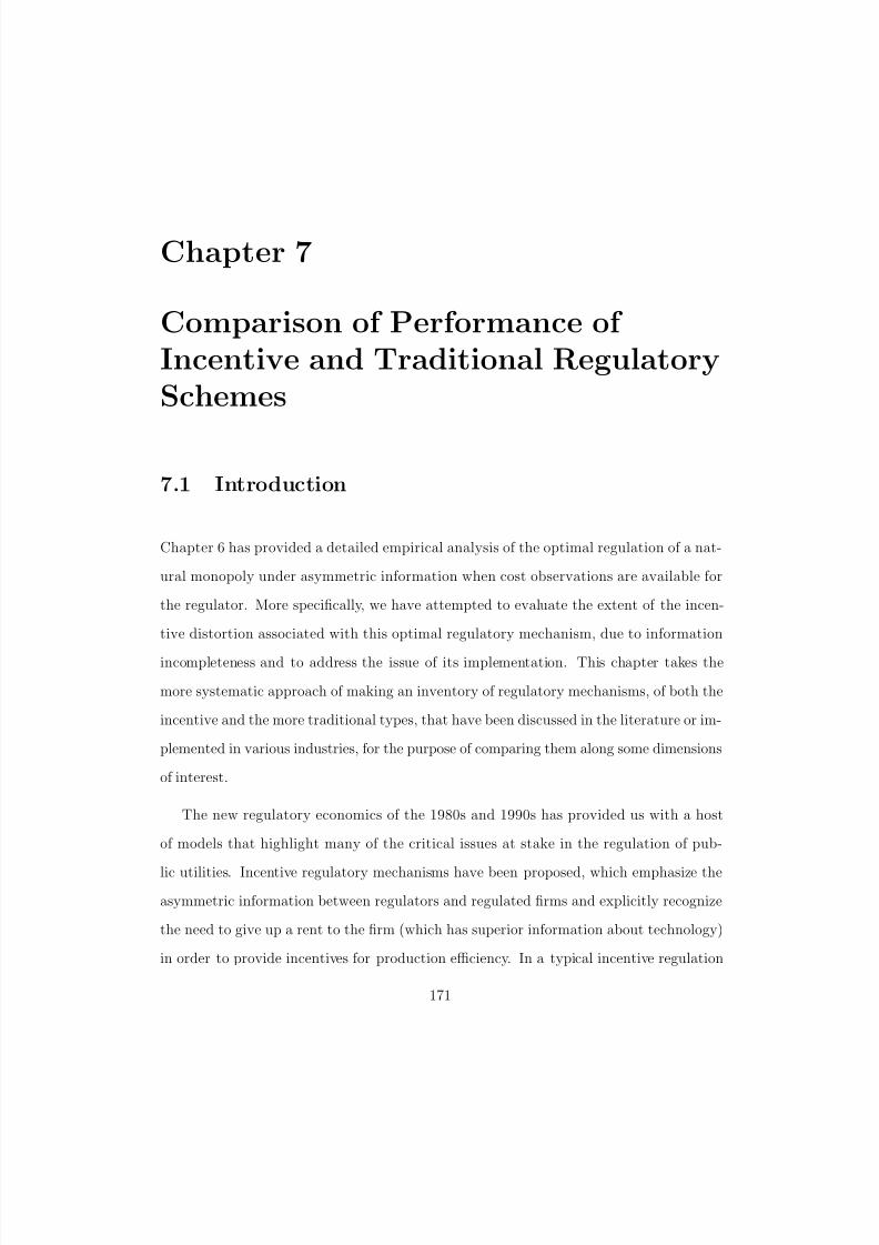
8/18/2019 Gasmi Cost Proxy Models
http://slidepdf.com/reader/full/gasmi-cost-proxy-models 171/318
Chapter 7
Comparison of Performance of
Incentive and Traditional RegulatorySchemes
7.1 Introduction
Chapter 6 has provided a detailed empirical analysis of the optimal regulation of a nat-
ural monopoly under asymmetric information when cost observations are available for
the regulator. More specifically, we have attempted to evaluate the extent of the incen-
tive distortion associated with this optimal regulatory mechanism, due to information
incompleteness and to address the issue of its implementation. This chapter takes the
more systematic approach of making an inventory of regulatory mechanisms, of both the
incentive and the more traditional types, that have been discussed in the literature or im-
plemented in various industries, for the purpose of comparing them along some dimensions
of interest.
The new regulatory economics of the 1980s and 1990s has provided us with a host
of models that highlight many of the critical issues at stake in the regulation of pub-
lic utilities. Incentive regulatory mechanisms have been proposed, which emphasize the
asymmetric information between regulators and regulated firms and explicitly recognize
the need to give up a rent to the firm (which has superior information about technology)
in order to provide incentives for production efficiency. In a typical incentive regulation
171
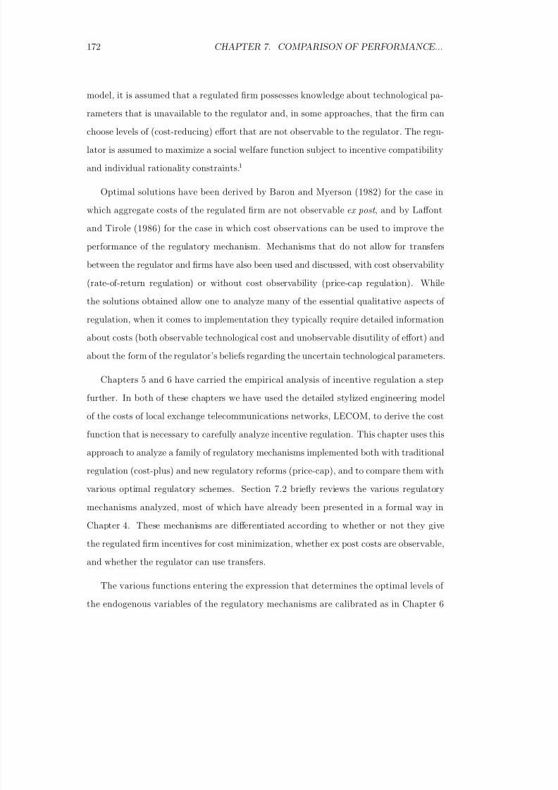
8/18/2019 Gasmi Cost Proxy Models
http://slidepdf.com/reader/full/gasmi-cost-proxy-models 172/318
172 CHAPTER 7. COMPARISON OF PERFORMANCE...
model, it is assumed that a regulated firm possesses knowledge about technological pa-
rameters that is unavailable to the regulator and, in some approaches, that the firm canchoose levels of (cost-reducing) effort that are not observable to the regulator. The regu-
lator is assumed to maximize a social welfare function subject to incentive compatibility
and individual rationality constraints.1
Optimal solutions have been derived by Baron and Myerson (1982) for the case in
which aggregate costs of the regulated firm are not observable ex post , and by Laffont
and Tirole (1986) for the case in which cost observations can be used to improve theperformance of the regulatory mechanism. Mechanisms that do not allow for transfers
between the regulator and firms have also been used and discussed, with cost observability
(rate-of-return regulation) or without cost observability (price-cap regulation). While
the solutions obtained allow one to analyze many of the essential qualitative aspects of
regulation, when it comes to implementation they typically require detailed information
about costs (both observable technological cost and unobservable disutility of effort) and
about the form of the regulator’s beliefs regarding the uncertain technological parameters.
Chapters 5 and 6 have carried the empirical analysis of incentive regulation a step
further. In both of these chapters we have used the detailed stylized engineering model
of the costs of local exchange telecommunications networks, LECOM, to derive the cost
function that is necessary to carefully analyze incentive regulation. This chapter uses this
approach to analyze a family of regulatory mechanisms implemented both with traditional
regulation (cost-plus) and new regulatory reforms (price-cap), and to compare them with
various optimal regulatory schemes. Section 7.2 briefly reviews the various regulatory
mechanisms analyzed, most of which have already been presented in a formal way in
Chapter 4. These mechanisms are differentiated according to whether or not they give
the regulated firm incentives for cost minimization, whether ex post costs are observable,
and whether the regulator can use transfers.
The various functions entering the expression that determines the optimal levels of
the endogenous variables of the regulatory mechanisms are calibrated as in Chapter 6
8/18/2019 Gasmi Cost Proxy Models
http://slidepdf.com/reader/full/gasmi-cost-proxy-models 173/318
7.2. ALTERNATIVE REGULATORY REGIMES 173
and they, therefore, will not be recalled in this chapter. In Section 7.3, we present the
empirical results and discuss their main features. The comparisons of the alternativeregulatory regimes (presented in Section 7.4) are organized in three steps. In Section
7.4.1 we assess their relative performance in terms of expected social welfare. In Section
7.4.2 we analyze the redistributive consequences of the various forms of regulation. Section
7.4.3 presents the results and implications of a sensitivity analysis of the performance of
the mechanisms with respect to the cost of public funds. We summarize our findings in a
concluding section (Section 7.5).
7.2 Alternative Regulatory Regimes
The various regulatory regimes analyzed in this chapter are described by means of some
basic theoretical ingredients which have been presented in the previous chapters. For
the purpose of evaluating the performance of regulation, it is worth recalling that, in
our framework, the basic objective function of the regulator is a utilitarian social welfarefunction (the sum of the consumers’ and the firm’s welfare) which can be written as
W = V (q ) − (1 + λ)[C (β, e, q ) + ψ(e)] − λU. (7.1)
where V (q ) is social value of the production q , C is the firm’s cost function, β is a
technological parameter, e is effort, ψ is the firm’s disutility of effort function, U is the
firm’s utility level and λ is the cost of public funds. Except for values of β , on which he has
some beliefs, and e, which he cannot observe, the regulator is assumed to have complete
information about this objective function (that is, the regulator knows the demand, cost
and disutility functions).2
The incomplete information regulatory mechanisms considered in this chapter are
characterized by various kinds of institutional assumptions that constrain their perfor-
mance relative to a complete information situation. It is then useful to derive a complete
information regulation which we use as a benchmark in our comparisons. This regulatory

8/18/2019 Gasmi Cost Proxy Models
http://slidepdf.com/reader/full/gasmi-cost-proxy-models 174/318
174 CHAPTER 7. COMPARISON OF PERFORMANCE...
solution, that we call C I , is found by solving for output, effort and utility levels q , e and
U that maximize social welfare given in (7.1) under the participation constraint that alltypes of firms achieve non-negative utility. Clearly, the participation constraint is binding
and the problem reduces to finding q and e that maximize
W CI = V (q ) − (1 + λ)[C (β, e, q ) + ψ(e)]. (7.2)
The formal representation of the various regulatory mechanisms we consider is given
in Chapter 4 in which we also discuss some of their important qualitative properties.3
Table 7.1 below gives a brief description of these regulatory schemes. These schemes are
subject to constraints of three types. Mechanisms differ in the (ex post) observability of
costs, in the feasibility of lump-sum transfers to the firm, and in the degree of bounded
rationality of the regulator (in addressing incentive issues). Therefore, conceptually, the
mechanisms can be visualized in a pair of two-dimensional transfer-observability diagrams
as shown in Figure 7.1. Along the transfer axis there are three possibilities: no transfers,
one-way transfers, and two-way transfers. Along the observability axis there is (ex post)
cost observability and effort observability (which applies only to the complete-information
benchmark).
8/18/2019 Gasmi Cost Proxy Models
http://slidepdf.com/reader/full/gasmi-cost-proxy-models 175/318
7.2. ALTERNATIVE REGULATORY REGIMES 175
Table 7.1Description of the regulatory mechanisms
Description Shorthand codeComplete information benchmark CI
Incomplete information optimal regulation LT with cost observability and transfers
Incomplete information optimal regulation BM without cost observability and with transfers
Price-cap regulation with no cost observability P C
and no transfers
Price-cap regulation with sharing of earnings P CT with cost observability and one-way transfers
Cost-plus regulation with reimbursement of C +observable costs and no additional transfers(balanced budget)
Cost-plus regulation with transfers used C + T
to balance the firm’s budget
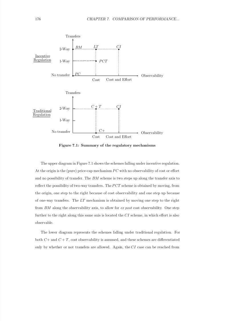
8/18/2019 Gasmi Cost Proxy Models
http://slidepdf.com/reader/full/gasmi-cost-proxy-models 176/318
176 CHAPTER 7. COMPARISON OF PERFORMANCE...
Transfers
2-Way
No transfer
LT CI
Cost Cost and EffortObservability
IncentiveRegulation
Transfers
Observability
2-Way
1-Way
No transfer
C + T
C +
TraditionalRegulation
P CT 1-Way
BM
P C
Cost Cost and Effort
CI
Figure 7.1: Summary of the regulatory mechanisms
The upper diagram in Figure 7.1 shows the schemes falling under incentive regulation.
At the origin is the (pure) price-cap mechanism P C with no observability of cost or effort
and no possibility of transfer. The BM scheme is two steps up along the transfer axis to
reflect the possibility of two-way transfers. The P CT scheme is obtained by moving, from
the origin, one step to the right because of cost observability and one step up because
of one-way transfers. The LT mechanism is obtained by moving one step to the right
from BM along the observability axis, to allow for ex post cost observability. One step
further to the right along this same axis is located the CI scheme, in which effort is also
observable.
The lower diagram represents the schemes falling under traditional regulation. For
both C + and C + T , cost observability is assumed, and these schemes are differentiated
only by whether or not transfers are allowed. Again, the CI case can be reached from
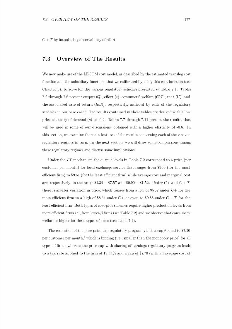
8/18/2019 Gasmi Cost Proxy Models
http://slidepdf.com/reader/full/gasmi-cost-proxy-models 177/318
7.3. OVERVIEW OF THE RESULTS 177
C + T by introducing observability of effort.
7.3 Overview of The Results
We now make use of the LECOM cost model, as described by the estimated translog cost
function and the subsidiary functions that we calibrated by using this cost function (see
Chapter 6), to solve for the various regulatory schemes presented in Table 7.1. Tables
7.2 through 7.6 present output (Q), effort (e), consumers’ welfare (CW ), rent (U ), and
the associated rate of return (RoR), respectively, achieved by each of the regulatory
schemes in our base case.4 The results contained in these tables are derived with a low
price-elasticity of demand (η) of -0.2. Tables 7.7 through 7.11 present the results, that
will be used in some of our discussions, obtained with a higher elasticity of -0.6. In
this section, we examine the main features of the results concerning each of these seven
regulatory regimes in turn. In the next section, we will draw some comparisons among
these regulatory regimes and discuss some implications.
Under the LT mechanism the output levels in Table 7.2 correspond to a price (per
customer per month) for local exchange service that ranges from $9.00 (for the most
efficient firm) to $9.61 (for the least efficient firm) while average cost and marginal cost
are, respectively, in the range $4.34 − $7.57 and $0.90 − $1.52. Under C + and C + T
there is greater variation in price, which ranges from a low of $5.62 under C + for the
most efficient firm to a high of $8.54 under C + or even to $9.88 under C + T for the
least efficient firm. Both types of cost-plus schemes require higher production levels from
more efficient firms i.e., from lower-β firms (see Table 7.2) and we observe that consumers’
welfare is higher for these types of firms (see Table 7.4).
The resolution of the pure price-cap regulatory program yields a cap ¯ p equal to $7.50
per customer per month,5 which is binding (i.e., smaller than the monopoly price) for all
types of firms, whereas the price-cap-with-sharing-of-earnings regulatory program leads
to a tax rate applied to the firm of 19.44% and a cap of $7.70 (with an average cost of
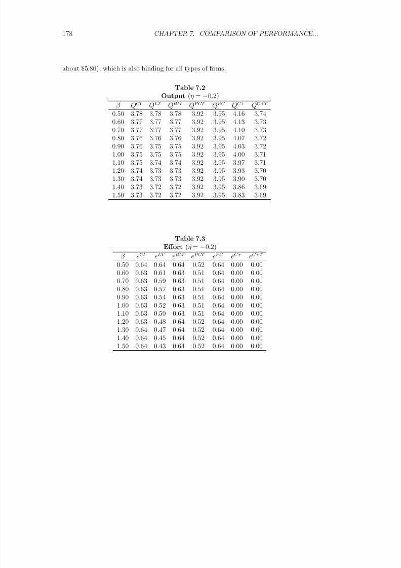
8/18/2019 Gasmi Cost Proxy Models
http://slidepdf.com/reader/full/gasmi-cost-proxy-models 178/318
178 CHAPTER 7. COMPARISON OF PERFORMANCE...
about $5.80), which is also binding for all types of firms.
Table 7.2Output (η = −0.2)
β QCI QLT QBM QP CT QP C QC + QC +T
0.50 3.78 3.78 3.78 3.92 3.95 4.16 3.740.60 3.77 3.77 3.77 3.92 3.95 4.13 3.730.70 3.77 3.77 3.77 3.92 3.95 4.10 3.730.80 3.76 3.76 3.76 3.92 3.95 4.07 3.720.90 3.76 3.75 3.75 3.92 3.95 4.03 3.721.00 3.75 3.75 3.75 3.92 3.95 4.00 3.711.10 3.75 3.74 3.74 3.92 3.95 3.97 3.711.20 3.74 3.73 3.73 3.92 3.95 3.93 3.701.30 3.74 3.73 3.73 3.92 3.95 3.90 3.701.40 3.73 3.72 3.72 3.92 3.95 3.86 3.691.50 3.73 3.72 3.72 3.92 3.95 3.83 3.69
Table 7.3Effort (η = −0.2)
β eCI eLT eBM eP CT eP C eC + eC +T
0.50 0.64 0.64 0.64 0.52 0.64 0.00 0.000.60 0.63 0.61 0.63 0.51 0.64 0.00 0.000.70 0.63 0.59 0.63 0.51 0.64 0.00 0.000.80 0.63 0.57 0.63 0.51 0.64 0.00 0.000.90 0.63 0.54 0.63 0.51 0.64 0.00 0.001.00 0.63 0.52 0.63 0.51 0.64 0.00 0.001.10 0.63 0.50 0.63 0.51 0.64 0.00 0.001.20 0.63 0.48 0.64 0.52 0.64 0.00 0.001.30 0.64 0.47 0.64 0.52 0.64 0.00 0.001.40 0.64 0.45 0.64 0.52 0.64 0.00 0.001.50 0.64 0.43 0.64 0.52 0.64 0.00 0.00
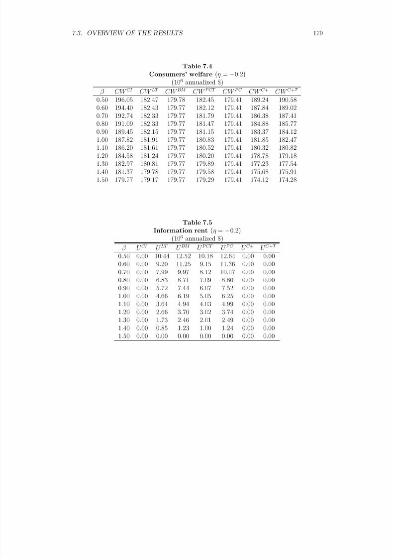
8/18/2019 Gasmi Cost Proxy Models
http://slidepdf.com/reader/full/gasmi-cost-proxy-models 179/318
7.3. OVERVIEW OF THE RESULTS 179
Table 7.4Consumers’ welfare (η = −0.2)
(106 annualized $)β CW CI CW LT CW BM CW P CT CW P C CW C + CW C +T
0.50 196.05 182.47 179.78 182.45 179.41 189.24 190.580.60 194.40 182.43 179.77 182.12 179.41 187.84 189.020.70 192.74 182.33 179.77 181.79 179.41 186.38 187.410.80 191.09 182.33 179.77 181.47 179.41 184.88 185.770.90 189.45 182.15 179.77 181.15 179.41 183.37 184.121.00 187.82 181.91 179.77 180.83 179.41 181.85 182.471.10 186.20 181.61 179.77 180.52 179.41 180.32 180.821.20 184.58 181.24 179.77 180.20 179.41 178.78 179.18
1.30 182.97 180.81 179.77 179.89 179.41 177.23 177.541.40 181.37 179.78 179.77 179.58 179.41 175.68 175.911.50 179.77 179.17 179.77 179.29 179.41 174.12 174.28
Table 7.5Information rent (η = −0.2)
(106 annualized $)
β U CI U LT U BM U P CT U P C U C + U C +T
0.50 0.00 10.44 12.52 10.18 12.64 0.00 0.000.60 0.00 9.20 11.25 9.15 11.36 0.00 0.000.70 0.00 7.99 9.97 8.12 10.07 0.00 0.000.80 0.00 6.83 8.71 7.09 8.80 0.00 0.000.90 0.00 5.72 7.44 6.07 7.52 0.00 0.001.00 0.00 4.66 6.19 5.05 6.25 0.00 0.001.10 0.00 3.64 4.94 4.03 4.99 0.00 0.001.20 0.00 2.66 3.70 3.02 3.74 0.00 0.001.30 0.00 1.73 2.46 2.01 2.49 0.00 0.00
1.40 0.00 0.85 1.23 1.00 1.24 0.00 0.001.50 0.00 0.00 0.00 0.00 0.00 0.00 0.00
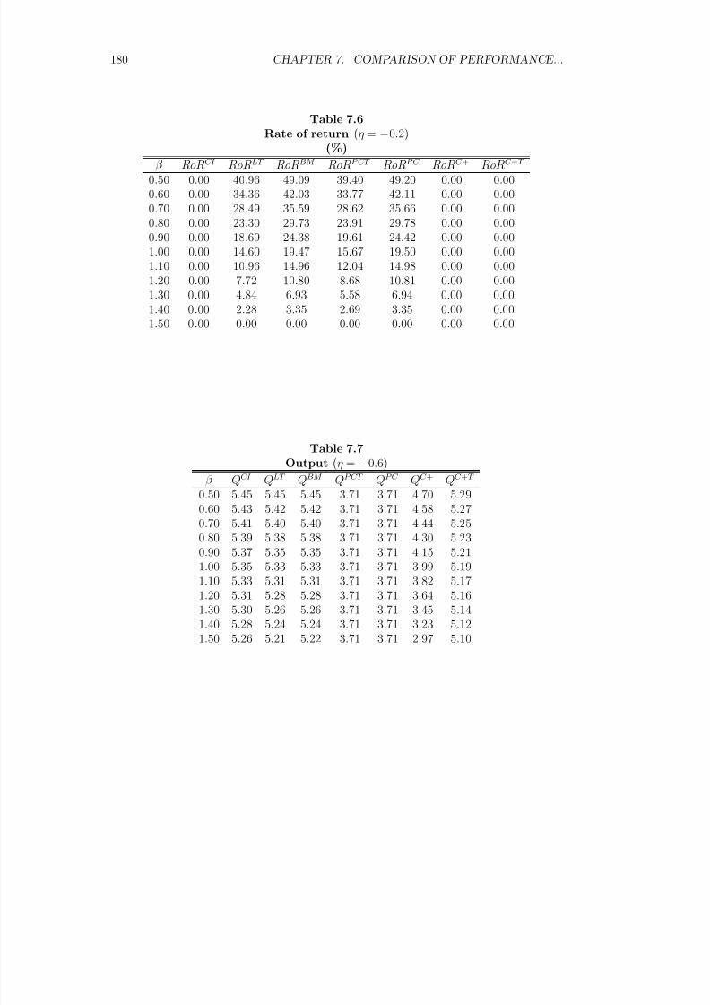
8/18/2019 Gasmi Cost Proxy Models
http://slidepdf.com/reader/full/gasmi-cost-proxy-models 180/318
180 CHAPTER 7. COMPARISON OF PERFORMANCE...
Table 7.6Rate of return (η = −0.2)
(%)β RoRCI RoRLT RoRBM RoRP CT RoRP C RoRC + RoRC +T
0.50 0.00 40.96 49.09 39.40 49.20 0.00 0.000.60 0.00 34.36 42.03 33.77 42.11 0.00 0.000.70 0.00 28.49 35.59 28.62 35.66 0.00 0.000.80 0.00 23.30 29.73 23.91 29.78 0.00 0.000.90 0.00 18.69 24.38 19.61 24.42 0.00 0.001.00 0.00 14.60 19.47 15.67 19.50 0.00 0.001.10 0.00 10.96 14.96 12.04 14.98 0.00 0.001.20 0.00 7.72 10.80 8.68 10.81 0.00 0.00
1.30 0.00 4.84 6.93 5.58 6.94 0.00 0.001.40 0.00 2.28 3.35 2.69 3.35 0.00 0.001.50 0.00 0.00 0.00 0.00 0.00 0.00 0.00
Table 7.7Output (η = −0.6)
β QCI QLT QBM QP CT QP C QC + QC +T
0.50 5.45 5.45 5.45 3.71 3.71 4.70 5.290.60 5.43 5.42 5.42 3.71 3.71 4.58 5.270.70 5.41 5.40 5.40 3.71 3.71 4.44 5.250.80 5.39 5.38 5.38 3.71 3.71 4.30 5.230.90 5.37 5.35 5.35 3.71 3.71 4.15 5.211.00 5.35 5.33 5.33 3.71 3.71 3.99 5.191.10 5.33 5.31 5.31 3.71 3.71 3.82 5.17
1.20 5.31 5.28 5.28 3.71 3.71 3.64 5.161.30 5.30 5.26 5.26 3.71 3.71 3.45 5.141.40 5.28 5.24 5.24 3.71 3.71 3.23 5.121.50 5.26 5.21 5.22 3.71 3.71 2.97 5.10
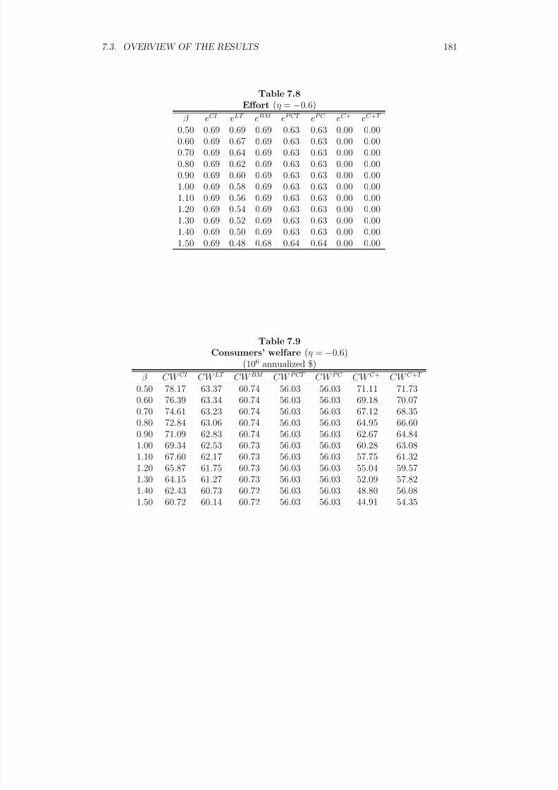
8/18/2019 Gasmi Cost Proxy Models
http://slidepdf.com/reader/full/gasmi-cost-proxy-models 181/318
7.3. OVERVIEW OF THE RESULTS 181
Table 7.8Effort (η = −0.6)
β eCI eLT eBM eP CT eP C eC + eC +T
0.50 0.69 0.69 0.69 0.63 0.63 0.00 0.000.60 0.69 0.67 0.69 0.63 0.63 0.00 0.000.70 0.69 0.64 0.69 0.63 0.63 0.00 0.000.80 0.69 0.62 0.69 0.63 0.63 0.00 0.000.90 0.69 0.60 0.69 0.63 0.63 0.00 0.001.00 0.69 0.58 0.69 0.63 0.63 0.00 0.001.10 0.69 0.56 0.69 0.63 0.63 0.00 0.001.20 0.69 0.54 0.69 0.63 0.63 0.00 0.001.30 0.69 0.52 0.69 0.63 0.63 0.00 0.00
1.40 0.69 0.50 0.69 0.63 0.63 0.00 0.001.50 0.69 0.48 0.68 0.64 0.64 0.00 0.00
Table 7.9
Consumers’ welfare (η = −0.6)(106 annualized $)
β CW CI CW LT CW BM CW P CT CW P C CW C + CW C +T
0.50 78.17 63.37 60.74 56.03 56.03 71.11 71.730.60 76.39 63.34 60.74 56.03 56.03 69.18 70.070.70 74.61 63.23 60.74 56.03 56.03 67.12 68.350.80 72.84 63.06 60.74 56.03 56.03 64.95 66.600.90 71.09 62.83 60.74 56.03 56.03 62.67 64.841.00 69.34 62.53 60.73 56.03 56.03 60.28 63.081.10 67.60 62.17 60.73 56.03 56.03 57.75 61.32
1.20 65.87 61.75 60.73 56.03 56.03 55.04 59.571.30 64.15 61.27 60.73 56.03 56.03 52.09 57.821.40 62.43 60.73 60.72 56.03 56.03 48.80 56.081.50 60.72 60.14 60.72 56.03 56.03 44.91 54.35
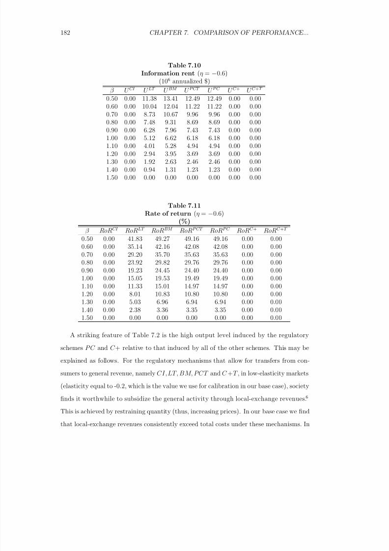
8/18/2019 Gasmi Cost Proxy Models
http://slidepdf.com/reader/full/gasmi-cost-proxy-models 182/318
182 CHAPTER 7. COMPARISON OF PERFORMANCE...
Table 7.10Information rent (η = −0.6)
(106 annualized $)β U CI U LT U BM U P CT U P C U C + U C +T
0.50 0.00 11.38 13.41 12.49 12.49 0.00 0.000.60 0.00 10.04 12.04 11.22 11.22 0.00 0.000.70 0.00 8.73 10.67 9.96 9.96 0.00 0.000.80 0.00 7.48 9.31 8.69 8.69 0.00 0.000.90 0.00 6.28 7.96 7.43 7.43 0.00 0.001.00 0.00 5.12 6.62 6.18 6.18 0.00 0.001.10 0.00 4.01 5.28 4.94 4.94 0.00 0.001.20 0.00 2.94 3.95 3.69 3.69 0.00 0.00
1.30 0.00 1.92 2.63 2.46 2.46 0.00 0.001.40 0.00 0.94 1.31 1.23 1.23 0.00 0.001.50 0.00 0.00 0.00 0.00 0.00 0.00 0.00
Table 7.11Rate of return (η = −0.6)
(%)
β RoRCI RoRLT RoRBM RoRP CT RoRP C RoRC + RoRC +T
0.50 0.00 41.83 49.27 49.16 49.16 0.00 0.000.60 0.00 35.14 42.16 42.08 42.08 0.00 0.000.70 0.00 29.20 35.70 35.63 35.63 0.00 0.000.80 0.00 23.92 29.82 29.76 29.76 0.00 0.000.90 0.00 19.23 24.45 24.40 24.40 0.00 0.001.00 0.00 15.05 19.53 19.49 19.49 0.00 0.001.10 0.00 11.33 15.01 14.97 14.97 0.00 0.001.20 0.00 8.01 10.83 10.80 10.80 0.00 0.001.30 0.00 5.03 6.96 6.94 6.94 0.00 0.001.40 0.00 2.38 3.36 3.35 3.35 0.00 0.001.50 0.00 0.00 0.00 0.00 0.00 0.00 0.00
A striking feature of Table 7.2 is the high output level induced by the regulatory
schemes P C and C + relative to that induced by all of the other schemes. This may be
explained as follows. For the regulatory mechanisms that allow for transfers from con-
sumers to general revenue, namely CI,LT, BM, PCT and C +T , in low-elasticity markets
(elasticity equal to -0.2, which is the value we use for calibration in our base case), society
finds it worthwhile to subsidize the general activity through local-exchange revenues.6
This is achieved by restraining quantity (thus, increasing prices). In our base case we find
that local-exchange revenues consistently exceed total costs under these mechanisms. In
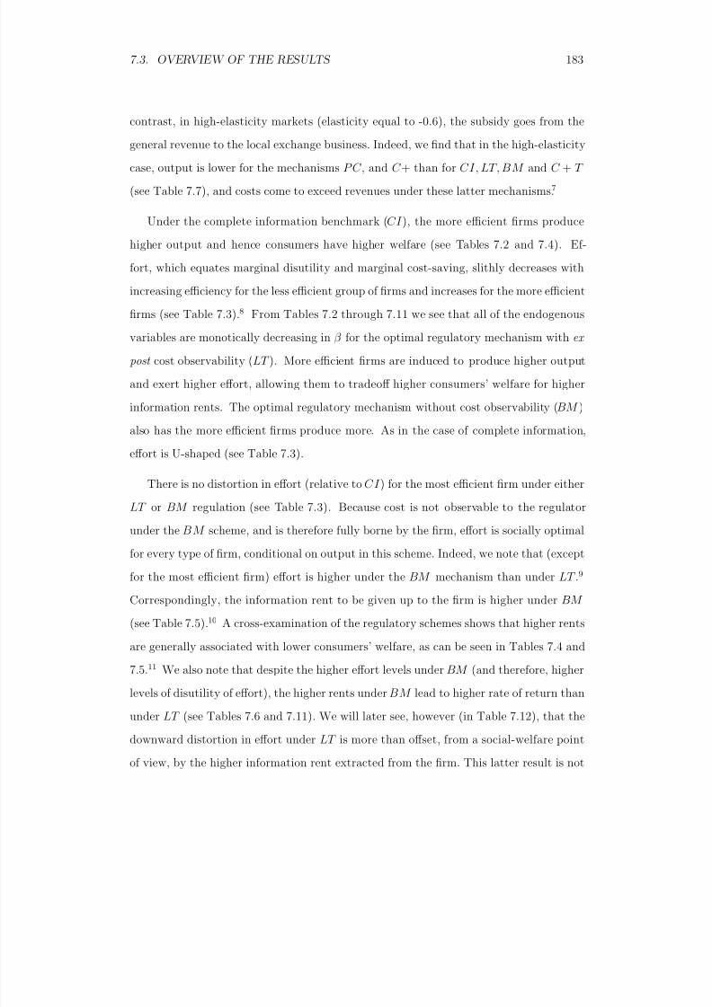
8/18/2019 Gasmi Cost Proxy Models
http://slidepdf.com/reader/full/gasmi-cost-proxy-models 183/318
7.3. OVERVIEW OF THE RESULTS 183
contrast, in high-elasticity markets (elasticity equal to -0.6), the subsidy goes from the
general revenue to the local exchange business. Indeed, we find that in the high-elasticitycase, output is lower for the mechanisms P C , and C + than for CI, LT, BM and C + T
(see Table 7.7), and costs come to exceed revenues under these latter mechanisms.7
Under the complete information benchmark (CI ), the more efficient firms produce
higher output and hence consumers have higher welfare (see Tables 7.2 and 7.4). Ef-
fort, which equates marginal disutility and marginal cost-saving, slithly decreases with
increasing efficiency for the less efficient group of firms and increases for the more efficientfirms (see Table 7.3).8 From Tables 7.2 through 7.11 we see that all of the endogenous
variables are monotically decreasing in β for the optimal regulatory mechanism with ex
post cost observability (LT ). More efficient firms are induced to produce higher output
and exert higher effort, allowing them to tradeoff higher consumers’ welfare for higher
information rents. The optimal regulatory mechanism without cost observability (BM )
also has the more efficient firms produce more. As in the case of complete information,
effort is U-shaped (see Table 7.3).
There is no distortion in effort (relative to C I ) for the most efficient firm under either
LT or BM regulation (see Table 7.3). Because cost is not observable to the regulator
under the B M scheme, and is therefore fully borne by the firm, effort is socially optimal
for every type of firm, conditional on output in this scheme. Indeed, we note that (except
for the most efficient firm) effort is higher under the BM mechanism than under LT .9
Correspondingly, the information rent to be given up to the firm is higher under BM
(see Table 7.5).10 A cross-examination of the regulatory schemes shows that higher rents
are generally associated with lower consumers’ welfare, as can be seen in Tables 7.4 and
7.5.11 We also note that despite the higher effort levels under BM (and therefore, higher
levels of disutility of effort), the higher rents under BM lead to higher rate of return than
under LT (see Tables 7.6 and 7.11). We will later see, however (in Table 7.12), that the
downward distortion in effort under LT is more than offset, from a social-welfare point
of view, by the higher information rent extracted from the firm. This latter result is not

8/18/2019 Gasmi Cost Proxy Models
http://slidepdf.com/reader/full/gasmi-cost-proxy-models 184/318
184 CHAPTER 7. COMPARISON OF PERFORMANCE...
surprising, since the option of ignoring cost observations is also available to the regulator
under the scheme.
Under P CT , part of the financial profits of the firm are returned to society. Con-
sequently, the firm exerts lower effort than under pure price cap P C (see Table 7.3 for
the low-elasticity case since for the high-elasticity case P C and P CT coincide.). The
sharing mechanism leads to lower rents and rates of return (see Tables 7.5 and 7.6), and
consumers’ welfare is higher (Table 7.4).
To conclude this broad presentation of the data produced by the resolution of the var-
ious regulatory schemes, we assess the relative importance of transfers from the regulator
to the firm under the optimal regulatory mechanism LT . Recall that the firm’s rent U ,
given by
U = t − ψ(e), (7.3)
where t is the net transfer and ψ is the disutility of effort, can be written in terms of the
gross transfer t as
U = t + pq − C − ψ. (7.4)
If transfers were not explicitly allowed, they still could be operated through a two-part
tariff T = A + pq .12 The fixed part A would then have to be set equal to the gross transfer
t and by (7.3) we would have:
A = t = t + C − pq. (7.5)
We have calculated A for both the low (-0.2) and high (-0.6) elasticity of demand cases.
The results showed an average subsidy of $6.50 per customer per month in the case of
low elasticity and an average charge of about $10.90 in the case of high elasticity.
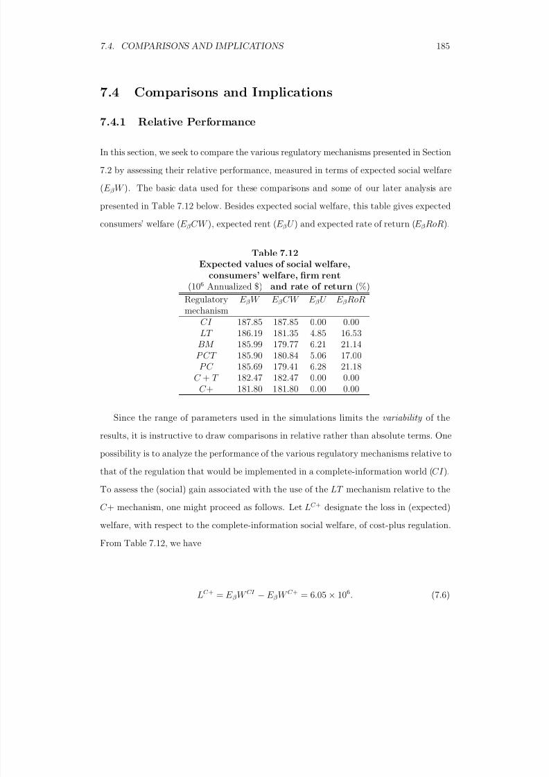
8/18/2019 Gasmi Cost Proxy Models
http://slidepdf.com/reader/full/gasmi-cost-proxy-models 185/318
7.4. COMPARISONS AND IMPLICATIONS 185
7.4 Comparisons and Implications
7.4.1 Relative Performance
In this section, we seek to compare the various regulatory mechanisms presented in Section
7.2 by assessing their relative performance, measured in terms of expected social welfare
(E β W ). The basic data used for these comparisons and some of our later analysis are
presented in Table 7.12 below. Besides expected social welfare, this table gives expected
consumers’ welfare (E β CW ), expected rent (E β U ) and expected rate of return (E β RoR).
Table 7.12Expected values of social welfare,
consumers’ welfare, firm rent(106 Annualized $) and rate of return (%)
Regulatory E β W E β CW E β U E β RoRmechanism
CI 187.85 187.85 0.00 0.00LT 186.19 181.35 4.85 16.53
BM 185.99 179.77 6.21 21.14P CT 185.90 180.84 5.06 17.00P C 185.69 179.41 6.28 21.18
C + T 182.47 182.47 0.00 0.00C + 181.80 181.80 0.00 0.00
Since the range of parameters used in the simulations limits the variability of the
results, it is instructive to draw comparisons in relative rather than absolute terms. One
possibility is to analyze the performance of the various regulatory mechanisms relative tothat of the regulation that would be implemented in a complete-information world (CI ).
To assess the (social) gain associated with the use of the LT mechanism relative to the
C + mechanism, one might proceed as follows. Let LC + designate the loss in (expected)
welfare, with respect to the complete-information social welfare, of cost-plus regulation.
From Table 7.12, we have
LC + = E β W CI − E β W C + = 6.05 × 10⁶. (7.6)
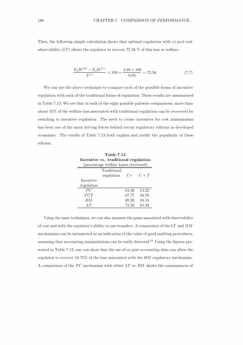
8/18/2019 Gasmi Cost Proxy Models
http://slidepdf.com/reader/full/gasmi-cost-proxy-models 186/318
186 CHAPTER 7. COMPARISON OF PERFORMANCE...
Then, the following simple calculation shows that optimal regulation with ex post cost
observability (LT ) allows the regulator to recover 72.56 % of this loss in welfare:
E β W LT − E β W C +
LC + × 100 =
4.39 × 100
6.05 = 72.56. (7.7)
We can use the above technique to compare each of the possible forms of incentive
regulation with each of the traditional forms of regulation. These results are summarized
in Table 7.13. We see that in each of the eight possible pairwise comparisons, more than
about 55% of the welfare loss associated with traditional regulation can be recovered by
switching to incentive regulation. The need to create incentives for cost minimization
has been one of the main driving forces behind recent regulatory reforms in developed
economies. The results of Table 7.13 both explain and justify the popularity of these
reforms.
Table 7.13Incentive vs. traditional regulation
(percentage welfare losses recovered)
Traditionalregulation C + C + T
Incentiveregulation
P C 64.30 53.22P CT 67.77 56.70BM 69.26 58.18LT 72.56 61.49
Using the same techniques, we can also measure the gains associated with observability
of cost and with the regulator’s ability to use transfers. A comparison of the LT and BM
mechanisms can be interpreted as an indication of the value of good auditing procedures,
assuming that accounting manipulations can be easily detected.13 Using the figures pre-
sented in Table 7.12, one can show that the use of ex post accounting data can allow the
regulator to recover 10.75% of the loss associated with the BM regulatory mechanism.
A comparison of the P C mechanism with either LT or BM shows the consequences of
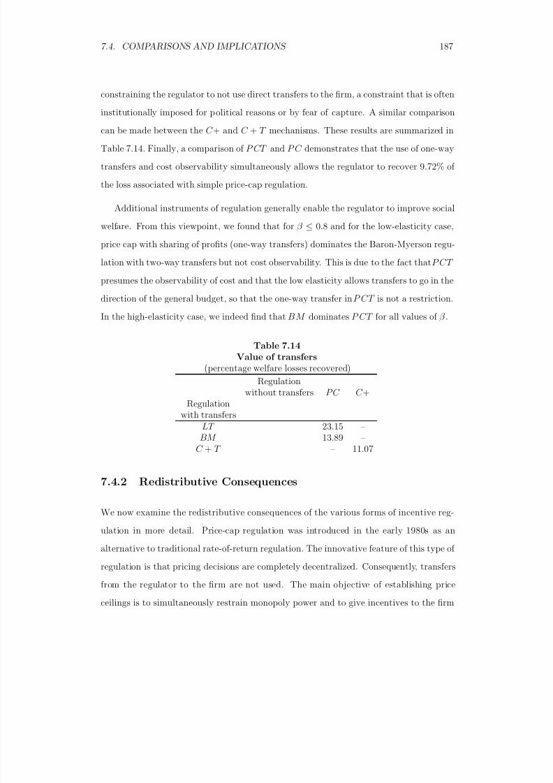
8/18/2019 Gasmi Cost Proxy Models
http://slidepdf.com/reader/full/gasmi-cost-proxy-models 187/318
7.4. COMPARISONS AND IMPLICATIONS 187
constraining the regulator to not use direct transfers to the firm, a constraint that is often
institutionally imposed for political reasons or by fear of capture. A similar comparisoncan be made between the C + and C + T mechanisms. These results are summarized in
Table 7.14. Finally, a comparison of P CT and P C demonstrates that the use of one-way
transfers and cost observability simultaneously allows the regulator to recover 9.72% of
the loss associated with simple price-cap regulation.
Additional instruments of regulation generally enable the regulator to improve social
welfare. From this viewpoint, we found that for β ≤ 0.8 and for the low-elasticity case,price cap with sharing of profits (one-way transfers) dominates the Baron-Myerson regu-
lation with two-way transfers but not cost observability. This is due to the fact that P CT
presumes the observability of cost and that the low elasticity allows transfers to go in the
direction of the general budget, so that the one-way transfer in P CT is not a restriction.
In the high-elasticity case, we indeed find that B M dominates P CT for all values of β .
Table 7.14Value of transfers
(percentage welfare losses recovered)
Regulationwithout transfers P C C +
Regulationwith transfers
LT 23.15 –BM 13.89 –
C + T – 11.07
7.4.2 Redistributive Consequences
We now examine the redistributive consequences of the various forms of incentive reg-
ulation in more detail. Price-cap regulation was introduced in the early 1980s as an
alternative to traditional rate-of-return regulation. The innovative feature of this type of
regulation is that pricing decisions are completely decentralized. Consequently, transfers
from the regulator to the firm are not used. The main objective of establishing price
ceilings is to simultaneously restrain monopoly power and to give incentives to the firm
8/18/2019 Gasmi Cost Proxy Models
http://slidepdf.com/reader/full/gasmi-cost-proxy-models 188/318
188 CHAPTER 7. COMPARISON OF PERFORMANCE...
for cost minimization. Indeed, because under price cap the firm is the residual claimant
of any cost reductions, much efficiency is achieved with P C as higher effort and quantitylevels than under either BM or LT are induced (see Tables 7.2 and 7.3). The pitfall
associated with P C , however, is that higher rents (see Tables 7.5 and 7.12) and rates
of return (see Tables 7.6 and 7.12) are realized by the firm, leading to lower consumer
welfare (see Tables 7.4 and 7.12) and social welfare (see Table 7.12). Thus, the efficiency
achieved through decentralization comes at a social cost.
Given the high performance of the P C mechanism in terms of incentives for efficiency,profit-sharing rules have been introduced to improve its working in terms of rent extrac-
tion. The direct comparison of the P C and P CT mechanisms in Table 7.12 and in the
above discussion, however, suggests that the gains associated with the use of transfers to
the firm and cost observability (equal to 9.72 % of the difference between aggregate welfare
under CI and P C ) are relatively modest, particularly when compared to the substantial
gains associated with adopting any form of incentive regulation over traditional regula-
tion. How then are we to explain the wide use of sharing rules whenever price-cap forms
of regulation are adopted? The answer may lie in a deeper analysis of the distributional
consequences of imposing incentive regulation.
Figure 7.2 below illustrates the trade-off between consumers’ welfare and rent under
alternative forms of regulation. Although consumers benefit most from cost-plus regula-
tion, expected social welfare is lowest under this traditional form of regulation. In other
words, if higher social welfare is the main objective, to achieve this goal through higher
production efficiency, society needs to sacrifice consumer welfare in favor of rents. This
fundamental trade-off is shown in Figure 7.2, which reports the (ex ante) distribution of
social welfare between consumers (surplus) and the firm (rent) under each of the regula-
tory regimes. This figure may provide some empirical substance to a positive theory of the
resistance of various interest groups to certain forms of regulation, which, in particular,
would predict that incentive regulation is promoted by firms.

8/18/2019 Gasmi Cost Proxy Models
http://slidepdf.com/reader/full/gasmi-cost-proxy-models 189/318
7.4. COMPARISONS AND IMPLICATIONS 189
178 180 182 184 186 188
-1
1
3
5
7
P C
BM
P CT LT
C + C + T CI
Consumers’ welfare
Rent
M$
M$
Figure 7.2: Rent-consumers’ welfare trade-off
We now present a more formal analysis of these issues. Recall that in all of the
regulatory mechanisms considered in Section 7.2, the objective of the regulator is the
maximization of a Benthamite social welfare function, i.e., the unweighted sum of con-
sumers’ and the firm’s welfares. A generalization of this objective, which assigns a weight
δ to the firm’s utility, has been suggested in the literature:14
GW = C W + δU. (7.8)
This generic welfare measure can be used to generate an incomplete information (second-
best) Pareto frontier. The regulator’s generalized objective function (GW ) then takes the
form
GW = {V (q ) − (1 + λ)[C (β, e, q ) + t]} + δU (7.9)
= V (q ) − (1 + λ)[C (β, e, q ) + ψ(e)] − (λ + 1 − δ )U, (7.10)
and, with cost observability and two-way transfers, its maximization under the incentive
compatibility and the (ex post) individual rationality constraints yields the following
program
maxq(·),e(·)
β
β V (q (β )) − (1 + λ)[C (β, e(β ), q (β )) + ψ(e(β ))]
+(λ + 1 − δ )F (β )
f (β )ψ(e(β ))
C β (β, e(β ), q (β )
C e(β, e(β ), q (β ))
f (β )dβ. (7.11)
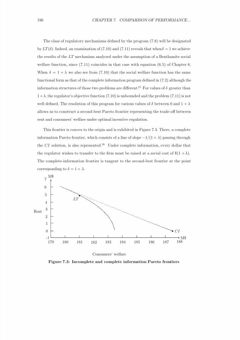
8/18/2019 Gasmi Cost Proxy Models
http://slidepdf.com/reader/full/gasmi-cost-proxy-models 190/318
190 CHAPTER 7. COMPARISON OF PERFORMANCE...
The class of regulatory mechanisms defined by the program (7.8) will be designated
by LT (δ ). Indeed, an examination of (7.10) and (7.11) reveals that when δ = 1 we achievethe results of the LT mechanism analyzed under the assumption of a Benthamite social
welfare function, since (7.11) coincides in that case with equation (6.5) of Chapter 6.
When δ = 1 + λ we also see from (7.10) that the social welfare function has the same
functional form as that of the complete information program defined in (7.2) although the
information structures of those two problems are different.15 For values of δ greater than
1 + λ, the regulator’s objective function (7.10) is unbounded and the problem (7.11) is not
well defined. The resolution of this program for various values of δ between 0 and 1 + λ
allows us to construct a second-best Pareto frontier representing the trade-off between
rent and consumers’ welfare under optimal incentive regulation.
This frontier is convex to the origin and is exhibited in Figure 7.3. There, a complete
information Pareto frontier, which consists of a line of slope −1/(1 + λ) passing through
the CI solution, is also represented.16 Under complete information, every dollar that
the regulator wishes to transfer to the firm must be raised at a social cost of $(1 + λ).
The complete-information frontier is tangent to the second-best frontier at the point
corresponding to δ = 1 + λ.
179 180 181 182 183 184 185 186 187
188
-1
0
1
2
3
4
5
6
7
LT
CI
Consumers’ welfare
Rent
M$
M$
Figure 7.3: Incomplete and complete information Pareto frontiers
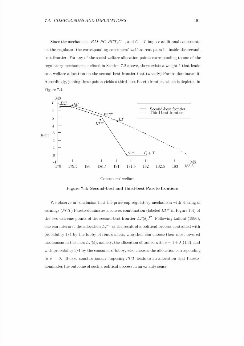
8/18/2019 Gasmi Cost Proxy Models
http://slidepdf.com/reader/full/gasmi-cost-proxy-models 191/318
7.4. COMPARISONS AND IMPLICATIONS 191
Since the mechanisms B M, PC , PC T, C +, and C + T impose additional constraints
on the regulator, the corresponding consumers’ welfare-rent pairs lie inside the second-best frontier. For any of the social-welfare allocation points corresponding to one of the
regulatory mechanisms defined in Section 7.2 above, there exists a weight δ that leads
to a welfare allocation on the second-best frontier that (weakly) Pareto-dominates it.
Accordingly, joining these points yields a third-best Pareto frontier, which is depicted in
Figure 7.4.
179 179.5 180 180.5 181 181.5 182 182.5 183
183.5
-1
0
1
2
3
4
5
6
7
Consumers’ welfare
Rent
P C BM
C + C + T
P CT LT
LT cc
Second-best frontierThird-best frontier
M$
M$
Figure 7.4: Second-best and third-best Pareto frontiers
We observe in conclusion that the price-cap regulatory mechanism with sharing of earnings (P CT ) Pareto-dominates a convex combination (labeled LT cc in Figure 7.4) of
the two extreme points of the second-best frontier LT (δ ).17 Following Laffont (1996),
one can interpret the allocation LT cc as the result of a political process controlled with
probability 1/4 by the lobby of rent owners, who then can choose their most favored
mechanism in the class LT (δ ), namely, the allocation obtained with δ = 1 + λ (1.3), and
with probability 3/4 by the consumers’ lobby, who chooses the allocation corresponding
to δ = 0. Hence, constitutionally imposing P CT leads to an allocation that Pareto-
dominates the outcome of such a political process in an ex ante sense.
8/18/2019 Gasmi Cost Proxy Models
http://slidepdf.com/reader/full/gasmi-cost-proxy-models 192/318
192 CHAPTER 7. COMPARISON OF PERFORMANCE...
7.4.3 Effect of The Cost of Public Funds
Because it reflects the social cost associated with transfers from consumers to the firm,
the parameter λ, referred to as the shadow cost of public funds, plays a crucial role in the
analysis of welfare. While a thorough study of the factors that determine this parameter
is beyond the scope of our current analysis, we expect its value to be higher for economies
with less efficient taxation systems, such as developing countries. In the next exercise, we
seek to investigate empirically how this parameter affects regulatory outcomes for both
low-elasticity and high-elasticity markets.
Tables 7.15 and 7.16 summarize the results of the computation of expected social
welfare for each of the seven regulatory mechanisms for various values of the cost of public
funds, assuming low (-0.2) and high (-0.6) demand elasticities, respectively. For each of
the regulatory mechanisms that allow for a transfer from consumers to general revenue,
the performance of the mechanism will be sensitive to the cost of public funds. From
(7.2) we can see that the derivative of the complete information social welfare function
with respect to λ is given by
∂W
∂λ = pq − C − ψ. (7.12)
For small values of λ this quantity is negative (i.e., revenues are less than total cost),but as λ increases it becomes increasingly attractive to restrict quantities in order to
extract revenues from local-exchange telephone customers to subsidize the general budget.
Hence, the social-welfare function under complete information is U-shaped as a function
of λ.18 In the higher-elasticity example, it is more costly, in terms of foregone surplus, to
extract revenues from local-exchange consumers, and social welfare is therefore declining
with respect to λ over a larger range of values of λ. Similar observations apply to each of
the regulatory mechanisms involving transfers (although for LT and BM the effect shows
for values of λ greater than 1).
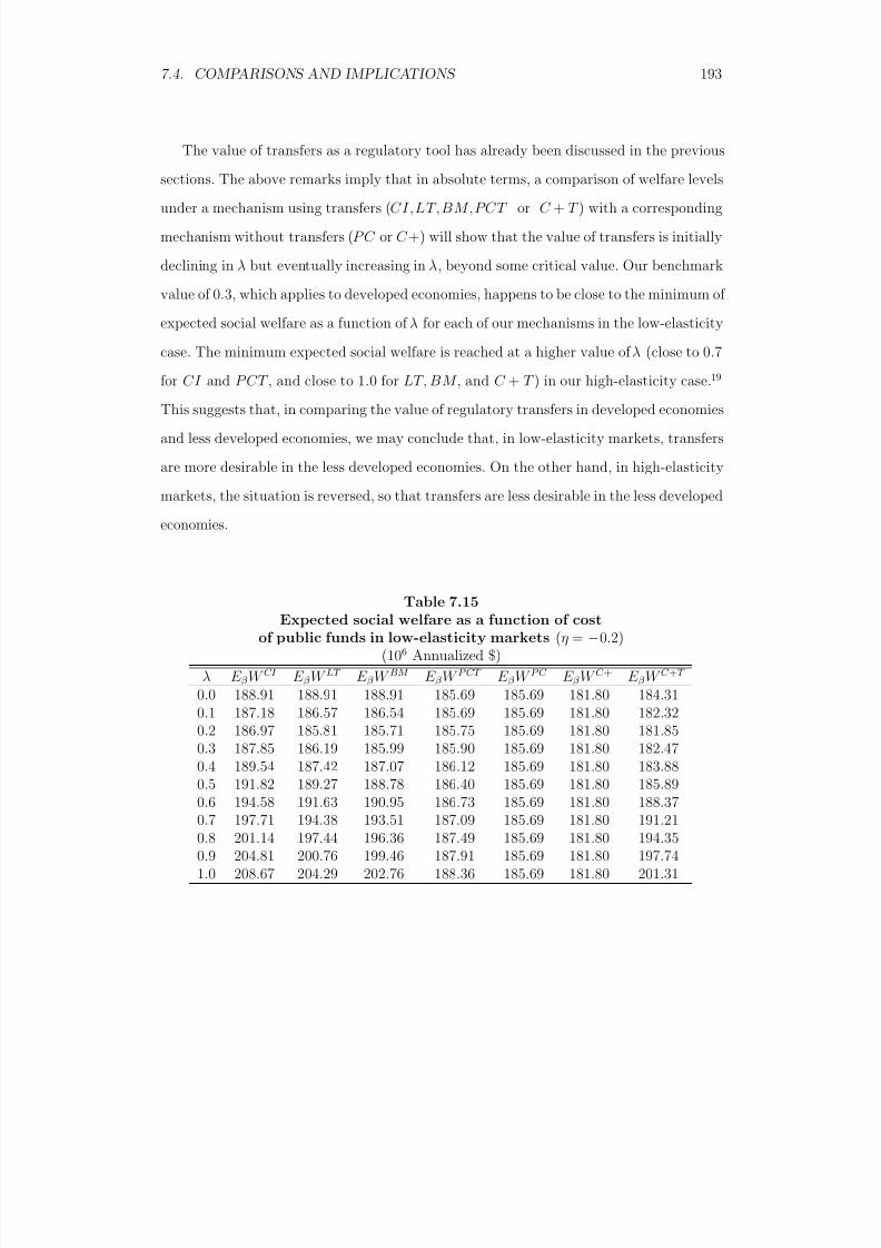
8/18/2019 Gasmi Cost Proxy Models
http://slidepdf.com/reader/full/gasmi-cost-proxy-models 193/318
7.4. COMPARISONS AND IMPLICATIONS 193
The value of transfers as a regulatory tool has already been discussed in the previous
sections. The above remarks imply that in absolute terms, a comparison of welfare levelsunder a mechanism using transfers (CI,LT,BM,PCT or C + T ) with a corresponding
mechanism without transfers (P C or C +) will show that the value of transfers is initially
declining in λ but eventually increasing in λ, beyond some critical value. Our benchmark
value of 0.3, which applies to developed economies, happens to be close to the minimum of
expected social welfare as a function of λ for each of our mechanisms in the low-elasticity
case. The minimum expected social welfare is reached at a higher value of λ (close to 0.7
for CI and P CT , and close to 1.0 for LT, BM , and C + T ) in our high-elasticity case.19
This suggests that, in comparing the value of regulatory transfers in developed economies
and less developed economies, we may conclude that, in low-elasticity markets, transfers
are more desirable in the less developed economies. On the other hand, in high-elasticity
markets, the situation is reversed, so that transfers are less desirable in the less developed
economies.
Table 7.15Expected social welfare as a function of cost
of public funds in low-elasticity markets (η = −0.2)(106 Annualized $)
λ E β W CI E β W LT E β W BM E β W P CT E β W P C E β W C + E β W C +T
0.0 188.91 188.91 188.91 185.69 185.69 181.80 184.310.1 187.18 186.57 186.54 185.69 185.69 181.80 182.32
0.2 186.97 185.81 185.71 185.75 185.69 181.80 181.850.3 187.85 186.19 185.99 185.90 185.69 181.80 182.470.4 189.54 187.42 187.07 186.12 185.69 181.80 183.880.5 191.82 189.27 188.78 186.40 185.69 181.80 185.890.6 194.58 191.63 190.95 186.73 185.69 181.80 188.370.7 197.71 194.38 193.51 187.09 185.69 181.80 191.210.8 201.14 197.44 196.36 187.49 185.69 181.80 194.350.9 204.81 200.76 199.46 187.91 185.69 181.80 197.741.0 208.67 204.29 202.76 188.36 185.69 181.80 201.31
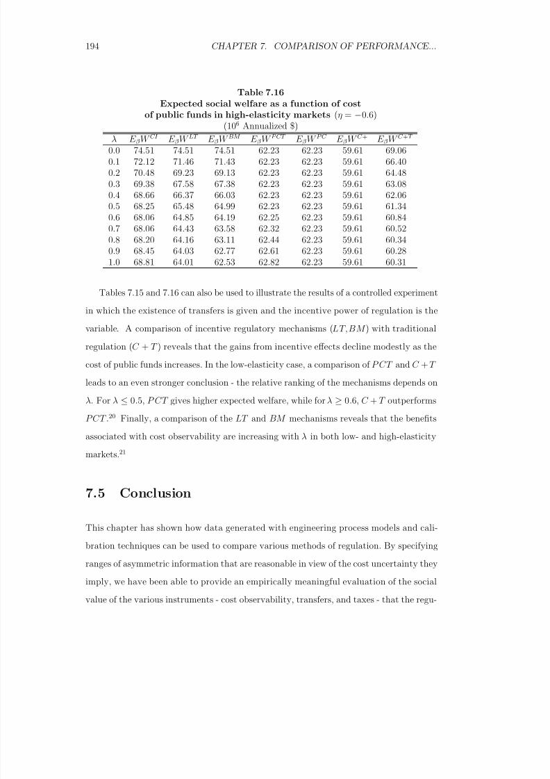
8/18/2019 Gasmi Cost Proxy Models
http://slidepdf.com/reader/full/gasmi-cost-proxy-models 194/318
194 CHAPTER 7. COMPARISON OF PERFORMANCE...
Table 7.16Expected social welfare as a function of cost
of public funds in high-elasticity markets (η = −0.6)(106 Annualized $)
λ E β W CI E β W LT E β W BM E β W P CT E β W P C E β W C + E β W C +T
0.0 74.51 74.51 74.51 62.23 62.23 59.61 69.060.1 72.12 71.46 71.43 62.23 62.23 59.61 66.400.2 70.48 69.23 69.13 62.23 62.23 59.61 64.480.3 69.38 67.58 67.38 62.23 62.23 59.61 63.080.4 68.66 66.37 66.03 62.23 62.23 59.61 62.060.5 68.25 65.48 64.99 62.23 62.23 59.61 61.340.6 68.06 64.85 64.19 62.25 62.23 59.61 60.84
0.7 68.06 64.43 63.58 62.32 62.23 59.61 60.520.8 68.20 64.16 63.11 62.44 62.23 59.61 60.340.9 68.45 64.03 62.77 62.61 62.23 59.61 60.281.0 68.81 64.01 62.53 62.82 62.23 59.61 60.31
Tables 7.15 and 7.16 can also be used to illustrate the results of a controlled experiment
in which the existence of transfers is given and the incentive power of regulation is the
variable. A comparison of incentive regulatory mechanisms (LT,BM ) with traditional
regulation (C + T ) reveals that the gains from incentive effects decline modestly as the
cost of public funds increases. In the low-elasticity case, a comparison of P CT and C + T
leads to an even stronger conclusion - the relative ranking of the mechanisms depends on
λ. For λ ≤ 0.5, P CT gives higher expected welfare, while for λ ≥ 0.6, C + T outperforms
P CT .20 Finally, a comparison of the LT and BM mechanisms reveals that the benefits
associated with cost observability are increasing with λ in both low- and high-elasticity
markets.
21
7.5 Conclusion
This chapter has shown how data generated with engineering process models and cali-
bration techniques can be used to compare various methods of regulation. By specifying
ranges of asymmetric information that are reasonable in view of the cost uncertainty they
imply, we have been able to provide an empirically meaningful evaluation of the social
value of the various instruments - cost observability, transfers, and taxes - that the regu-

8/18/2019 Gasmi Cost Proxy Models
http://slidepdf.com/reader/full/gasmi-cost-proxy-models 195/318
7.5. CONCLUSION 195
lator can use. Despite the drawbacks of the analysis (related, in particular, to the static
character of the model), we have illustrated some important results of the economics of regulation and derived some new empirical insights.
The trade-off between rent extraction and consumer’s surplus associated with the
various regulatory mechanisms has been exhibited, but also situated in a perspective of
general welfare analysis under incomplete information. The important role of the cost of
public funds in regulation and its implications for developing countries have been clearly
established. The usefulness of this type of normative analysis even for a positive approachto regulation has been illustrated.
Empirically, the most striking result is the reasonably good performance of price-cap
regulation combined with taxation of profits, which appears as the most practical tool
of implementation of a quasi-optimal regulation. Also, the empirical analysis reveals the
sensitivity of the results to the elasticity of demand and its implications for the possibility
of using the industry as an instrument of taxation.
8/18/2019 Gasmi Cost Proxy Models
http://slidepdf.com/reader/full/gasmi-cost-proxy-models 196/318
196 NOTES
Notes
1This normative approach should be viewed as a necessary first step. A more complete
approach should explictly take into account political constraints. In Section 7.4 of this
chapter, we refer to a reduced-form model based on this later type of approach.
2Note again that the expression of the social welfare function (7.1) shows that the
regulator dislikes leaving a rent to the firm. This will turn out to be an important
determinant of the optimal regulatory policies.
3The compact form of the optimal regulatory mechanism with transfers and cost ob-
servability (LT ) is given in the previous chapter. When costs are not observable it can
easily be shown that the regulatory program (BM ) can compactly be written as:
maxq(·)
β
β
V (q (β )) − (1 + λ)[C (β, e∗(β, q (β )), q (β )) + ψ(e∗(β, q (β )))]
−λF (β )
f (β )
C β (β, e∗(β, q (β )), q (β ))
f (β )dβ.
where e∗ refers to optimal effort and F (f ) is a cumulative distribution (density) that
describes the beliefs of the regulator concerning the technological parameter β .
4It is useful to recall here that (see also Chapter 4) C W = V (q )−(1+λ)(t+C (β, e, q )),
where V (q ) = S (q ) + λP (q )q and S (·) and P (·) are, respectively, the gross consumer
surplus and the inverse demand function, U = t−ψ(e), where t is the net monetary transfer
(if allowed) from the regulator to the firm. We also define RoR as RoR = 100.U/(C + ψ).
5With an average cost of about $5.50.
6The social value of transfers will be further discussed below.
7For CI, LT and BM costs exceed revenues except for the most efficient firms in this
high-elasticity case. Also, in this case P C and P CT coincide.
8Note that, given the first-order condition that defines effort in C I, B M, PC , and
P CT (ψ = C e), there is no compelling reason to expect, for general cost functions,
8/18/2019 Gasmi Cost Proxy Models
http://slidepdf.com/reader/full/gasmi-cost-proxy-models 197/318
NOTES 197
monotonicity of effort even if C βe > 0 (which is the case for our estimated translog
cost function, as can be seen from the sign of the coefficient of the cross-product terminvolving P K and P L in equation (6.7) of Chapter 6), because of the influence of the
production level on cost. In the case of LT , however, the first-order condition in effort
has an additional term that leads to a distortion of effort. Monotonicity of effort arises
then as a consequence of the optimal trade-off between rent extraction and efficient effort.
9The fact that in Tables 7.2 and 7.7 output levels are practically identical for BM and
LT is a result of rounding. Output levels are lower under B M , but the effect is small for
these particular simulations.
10Note that no rent is left for the least efficient firm under these mechanisms.
11Note, however, that for the highest-cost firms, rents are equal to zero under each form
of regulation and consumer welfare is higher under BM and P C regulation than under
LT and P CT regulation. The fundamental trade-offs involved in implementing incentive
regulation will be discussed further below.
12Note, however, that this would require a different interpretation of the dead-weight
loss associated with transfers, which here would have to allow for the possibility of dis-
connection of low-income consumers.
13If the project is small relative to the size of the firm, this assumption may fail to hold,
and cost observation may prove less useful than our computations suggest.
14See Baron (1989) for a good discussion of the rationale behind this specification.
15Under complete information, maximization is done with respect to q and e in which
effort e(β ) is assumed to be observable for any value of β . In contrast, under incomplete
information (i.e., on the second-best frontier), maximization is done with respect to the
functions q (β ) and e(β ) as in equation (6.5) of the previous chapter.
16Our quasilinear specification of utility functions leads to a linear Pareto frontier under
8/18/2019 Gasmi Cost Proxy Models
http://slidepdf.com/reader/full/gasmi-cost-proxy-models 198/318
198 NOTES
complete information. Furthermore, it limits the meaningfullness of δ to the highest value
of 1 + λ. For higher values the regulator would want to transfer unlimited amounts to thefirm. Asymmetric information typically convexifies the Pareto frontier, as transfers are
costly because of incentive constraints. See below some implication of this convexification
for the political economy of regulation.
17The point LT cc is obtained by giving weights 0.25 and 0.75 to the allocations on the
second-best frontier LT (δ ) corresponding to δ = 1.3 and δ = 0, respectively.
18The reader may be surprised by the fact that social welfare increases with high values
of λ. Note, however, that our social welfare function is only a partial one which does
not take into account the decrease of welfare elsewhere in the economy due to higher
inefficiencies in the tax system.
19For LT and BM the minimum is reached at a value of λ slightly greater than 1.
20
The situation is different in the high-elasticity case, where P CT outperforms C + T for λ ≥ 0.4.
21If moving to incentive regulation is viewed as an institutional innovation, this em-
pirical result confirms the ambiguity of the relative value of such innovations in LDCs
compared to developed countries discussed in Laffont and Meleu (1999).

8/18/2019 Gasmi Cost Proxy Models
http://slidepdf.com/reader/full/gasmi-cost-proxy-models 199/318
Chapter 8
Universal Service
8.1 Introduction
This chapter explores some practical aspects of a formidable challenge that faces the
telecommunications industry at the turn of the millenium: can the fundamental historical
goal set by countries, to provide a phone to anyone in any particular geographical area
who needs it, be fulfilled in the new information age characterized by a general trend
towards global deregulation of the industry? To be more specific, local telecommuni-
cations service has traditionally been provided by a monopoly under a regulated price
structure. In most countries and jurisdictions, an explicit goal of regulation has been the
provision of service to customers in high cost areas at “affordable” prices and this has
been achieved by cross-subsidies within the regulated monopoly. In recent years, however,
changing technologies and an increased appreciation of the benefits of competition in tra-
ditional natural monopoly industries have generated powerful forces for deregulation of
local telecommunications. These forces threaten the viability of this traditional method
of universal service funding. In this chapter, we empirically evaluate these trade-offs with
a special attention to parameter values that are relevant for developing economies.
The liberalization of telecommunications is proceeding at a pace faster than in most
other network industries. The issues of vertical disintegration, incentive regulation and ac-
cess pricing reform have been raised and dealt with in recent years. In telecommunications
199
8/18/2019 Gasmi Cost Proxy Models
http://slidepdf.com/reader/full/gasmi-cost-proxy-models 200/318
200 CHAPTER 8. UNIVERSAL SERVICE
the compatibility of competition and universal service obligations is the object of intense
political and economic debates. Competition destroys to a great extent cross-subsidiesso that some areas might be left with very high costs of provision of telecommunications
(maybe even the breakdown of provision) resulting in prices which are not considered
socially reasonable or affordable.
Various mechanisms have been proposed to fund, with tax money, the provision of
telecommunications in those areas in order to ensure universal service. However, in some
countries, and this is particularly so in less developed countries (LDCs), the tax system isvery inefficient, sometimes even corrupted, to the point where such transfers are socially
very costly. This raises the question of what is the best way to introduce competition
to limit the deadweight losses due to these transfers. The historical alternative has been
to finance the development of telecommunications in high cost areas from cross-subsidies
derived from the low cost areas with a regulated monopoly. More recently in Argentina,
the country has been divided in two regions, each one with an urban area and a rural area.
Cross-subsidies are maintained within each region, but some form of yardstick competition
exists between regions.1 Still some alternative competitive solutions might be envisionned
and one would like to compare those solutions for the new telecommunications technologies
and for various levels of efficiency of the tax systems. That is the issue explored in this
chapter.2
The rapid evolution of technologies prevents us from using field data and econometric
techniques to model the various technological and regulatory choices. Instead, as in pre-
vious chapters, we use the engineering simulation model LECOM to evaluate empirically
various complete and incomplete information regulatory schemes that ensure provision of
service in high cost areas. This methodology allows us to simulate the various asymme-
tries of information of the adverse selection or moral hazard type that play an important
role in the modern regulation literature.
Section 8.2 describes the various theoretical solutions that we wish to compare for
a community composed of an urban area and a rural area. Assuming first complete
8/18/2019 Gasmi Cost Proxy Models
http://slidepdf.com/reader/full/gasmi-cost-proxy-models 201/318
8.2. THE THEORETICAL ALTERNATIVES 201
information, we start with the (Hotelling) marginal-cost pricing solution supplemented
by costly transfers from the national budget in order to finance the implied deficit of thefirms. The implementation of this scheme in a duopoly setting enables us to compare
from a purely technological efficiency point of view the solution in which competitive
entry takes place in the (profitable) urban area only with the solution in which entry
is organized as a yardstick competition between two equal-size regions each of which is
composed of an urban area and a rural area.
Next, the relative performance of these solutions is reexamined when the regulatorrequires that the firms balance their budgets. We compare two regulatory scenarios. In
the first, entry is allowed in the urban sector and prices are unregulated, while a regulated
monopoly provides service in both urban and rural areas. In the second scenario, the
community is divided into two equal areas with balanced-budget provision within each
region and yardstick competition between regions. This step allows us to appraise the
consequences of the destruction of cross-subsidies due to urban competition (in the former
solution) and the value of a yardstick competition which maintains cross-subsidies (in the
latter solution). We then see how the availability of tax money affects the comparisons.
Finally, we explore how asymmetric information alters these comparisons.
Section 8.3 describes the way the cost proxy model LECOM (see Chapter 2) is used
to implement a simulation-calibration procedure. The empirical results are discussed and
summarized in Section 8.4 and Section 8.5 concludes the paper. An Appendix to the book
(Appendix A) presents additional data for each of the scenarios.
8.2 The Theoretical Alternatives
We consider a territory composed of two distinct areas, an urban area (area 1) and a rural
area (area 2), with N 1 and N 2 local telephone subscribers. For area i = 1, 2, we denote by
q i, P i(q i) and S i(q i), respectively, output (usage), the inverse demand function, and the
associated gross consumer surplus.3

8/18/2019 Gasmi Cost Proxy Models
http://slidepdf.com/reader/full/gasmi-cost-proxy-models 202/318
202 CHAPTER 8. UNIVERSAL SERVICE
Our first objective is to examine the relative technological efficiencies associated with
two alternative entry scenarios. The first scenario is an “Urban-Targeted” entry scenariolabelled U T in which entry, targeted towards the urban area only, leads to a split of the
urban market in half between the entrant and the incumbent. The latter also serves the
rural area. The second scenario is a “Territory-Constrained” entry scenario labelled T C in
which entry takes place in both the urban and rural areas, leading to an equal division of
both markets between the two firms. We initially examine these two scenarios by imposing
(socially efficient) marginal-cost pricing (mc) and financing with public subsidies ( ps) the
implied deficit in each case.4
The cost function of an integrated monopolistic firm serving the whole territority is
C = C (β, e, q 1, q 2 ; N 1, N 2) (8.1)
where β is a technological efficiency parameter belonging to an interval [β, β ] and e repre-
sents an endogenous efficiency parameter (the firm’s effort) which may take any nonneg-
ative value.5 The value of β is private information to the firm, but the regulator knows
the distribution function F (β ) and its density f (β ). An increase in the effort variable,
e, decreases observable cost, C , but also imposes a disutility ψ(e) on the firm’s manager
and workers. The level of effort carried out will depend upon the regulatory mechanism
implemented.
Under U T duopoly, the cost function of the incumbent (firm 1) that serves half of the
urban area and the whole rural area is
C U T 1 (β, e1, q 11, q 21) ≡ C (β, e1, q 11, q 21 ;
N 12
, N 2) (8.2)
where e1 is the incumbent’s effort and q 11 and q 21 is the incumbent’s output in the urban
area and the rural area respectively. The cost function of the entrant (firm 2) under this
scenario is
C U T 2 (β, e2, q 12) ≡ C (β, e2, q 12, 0 ;
N 12
, 0) (8.3)
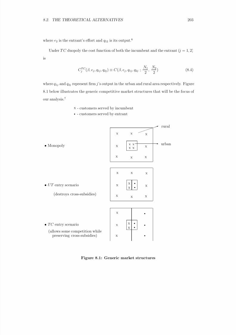
8/18/2019 Gasmi Cost Proxy Models
http://slidepdf.com/reader/full/gasmi-cost-proxy-models 203/318
8.2. THE THEORETICAL ALTERNATIVES 203
where e2 is the entrant’s effort and q 12 is its output.6
Under T C duopoly the cost function of both the incumbent and the entrant ( j = 1, 2)
is
C T C j (β, e j, q 1 j, q 2 j ) ≡ C (β, e j, q 1 j, q 2 j ;
N 12
, N 2
2 ) (8.4)
where q 1 j and q 2 j represent firm j’s output in the urban and rural area respectively. Figure
8.1 below illustrates the generic competitive market structures that will be the focus of
our analysis.7
x
x
x
x
x
xx
xx
x
x
x
x
xx
x
x x
x x
rural
urban
xx
x
x
x
xx
• Monopoly
• UT entry scenario
• T C entry scenario
x - customers served by incumbent - customers served by entrant
(destroys cross-subsidies)
(allows some competition whilepreserving cross-subsidies)
Figure 8.1: Generic market structures

8/18/2019 Gasmi Cost Proxy Models
http://slidepdf.com/reader/full/gasmi-cost-proxy-models 204/318
204 CHAPTER 8. UNIVERSAL SERVICE
As a benchmark case, let us first present the marginal-cost pricing schemes (supple-
mented by public subsidies) under the two types of equilibrium duopoly markets discussedabove. Scenario U T ps
mc features (regulated) competition targeted towards the urban sec-
tor in which we assume that an entrant captures half of the market and the incumbent
matches the entrant’s price at marginal cost. Accordingly, the incumbent serves the other
half as well as the whole rural area. The hypothesis of complete information allows the reg-
ulator to impose the optimal effort level on both the incumbent (e∗1) and the entrant (e∗2).8
Those firms solve, respectively, the first-order conditions which require that the marginal
disutility of effort for each firm be equal to the marginal benefit for cost-reducing activities
and prices to marginal costs. These conditions are represented in equation (8.5) through
(8.8) below where C U T 1 and C U T
2 are the cost functions of the incumbent and the entrant
defined in (8.2) and (8.3) respectively.9
ψ(e1) = −
∂C UT 1
∂e1
(β, e1, q
11, q
21) (8.5)
ψ(e2) = −∂C U T
2
∂e2
(β, e2, q 12) (8.6)
p1 = ∂C U T
2
∂q 12(β, e∗2, q 12) (8.7)
p2 = ∂C U T
1
∂q 2(β, e∗
1, q 11, q 21). (8.8)
Under our accounting convention, marginal-cost pricing creates an aggregate (finan-
cial) deficit, to be funded through public funds, given by
DU T psmc = C U T
1 (β, e∗1, q 1, q 21) + C UT 2 (β, e∗2, q 1) − N 1 p1q 1 − N 2 p2q 2 (8.9)
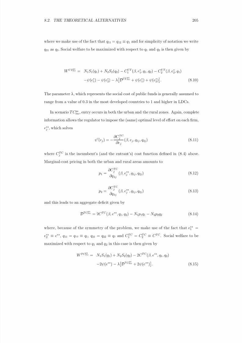
8/18/2019 Gasmi Cost Proxy Models
http://slidepdf.com/reader/full/gasmi-cost-proxy-models 205/318
8.2. THE THEORETICAL ALTERNATIVES 205
where we make use of the fact that q 11 = q 12 ≡ q 1 and for simplicity of notation we write
q 21 as q 2. Social welfare to be maximized with respect to q 1 and q 2 is then given by
W U T psmc = N 1S 1(q 1) + N 2S 2(q 2) − C U T
1 (β, e∗1, q 1, q 2) − C U T 2 (β, e∗2, q 1)
−ψ(e∗1) − ψ(e∗2) − λ
DUT psmc + ψ(e∗1) + ψ(e∗2)
. (8.10)
The parameter λ, which represents the social cost of public funds is generally assumed to
range from a value of 0.3 in the most developed countries to 1 and higher in LDCs.
In scenario T C psmc, entry occurs in both the urban and the rural zones. Again, complete
information allows the regulator to impose the (same) optimal level of effort on each firm,
e∗∗ j , which solves
ψ(e j ) = −∂C T C
j
∂e j
(β, e j, q 1 j , q 2 j) (8.11)
where C T C j is the incumbent’s (and the entrant’s) cost function defined in (8.4) above.
Marginal-cost pricing in both the urban and rural areas amounts to
p1 =∂C T C
j
∂q 1 j
(β, e∗∗ j , q 1 j, q 2 j ) (8.12)
p2 =∂C T C
j
∂q 2 j
(β, e∗∗ j , q 1 j, q 2 j ) (8.13)
and this leads to an aggregate deficit given by
DT C psmc = 2C T C (β, e∗∗, q 1, q 2) − N 1 p1q 1 − N 2 p2q 2 (8.14)
where, because of the symmetry of the problem, we make use of the fact that e∗∗1 =
e∗∗2 ≡ e∗∗, q 11 = q 12 ≡ q 1, q 21 = q 22 ≡ q 2 and C T C
1 = C T C 2 ≡ C T C . Social welfare to be
maximized with respect to q 1 and q 2 in this case is then given by
W T C psmc = N 1S 1(q 1) + N 2S 2(q 2) − 2C T C (β, e∗∗, q 1, q 2)
−2ψ(e∗∗) − λ
DT C psmc + 2ψ(e∗∗)
. (8.15)
8/18/2019 Gasmi Cost Proxy Models
http://slidepdf.com/reader/full/gasmi-cost-proxy-models 206/318
206 CHAPTER 8. UNIVERSAL SERVICE
Let us now turn to competitive alternatives. Under competition, the regulator does
not attempt to set either prices or effort levels. However, a profit-maximizing firm canbe assumed to select a competitive price (we assume Bertrand competition) and for each
price an optimal level of effort conditionally on the level of output. The regulator’s only
role is to enforce a market segmentation according to the UT or T C scenarios. Firms
must comply with the universal service obligation, i.e., the obligation to provide service
in (high cost) rural areas at an affordable price, which we take here as meaning the same
price as in urban areas.10 Second, we now impose a budget balance condition on the
regulated firm, and take account of the fact that public funds are a scarce resource. 11
First, we examine once again the framework in which entry occurs in the urban sector
only. Bertrand-like competition in the urban area is assumed to set the price of urban
service at the average cost of the entrant who serves one half of the market. If the incum-
bent matches this price in the urban area and serves the rural area at average (remaining)
cost, then cross-subsidies going from the urban to the rural sector are eliminated, but
the incumbent may not be able to satisfy the universal service obligation. 12 One way
to resolve this difficulty is to impose the urban price in the rural area and finance the
subsequent incumbent’s deficit through public subsidies. This is scenario UT psac that we
derive next.13
Optimal output of the entrant in the urban sector (which is also that of the incumbent)
q ∗1 (≡ q ∗11 = q ∗12) maximizes
N 12
S 1(q 1) − C U T 2 (β, e∗2, q 1) (8.16)
under the constraint
N 12
P 1(q 1)q 1 = C UT 2 (β, e∗2, q 1) + ψ(e∗2) (8.17)
where e∗2 is the entrant’s optimal effort level that satisfies (8.6). This yields the optimal
urban price p∗1 which is matched by the incumbent.14 The (residual) cost function for the
incumbent is
C U T 1 (β, e∗1, q ∗1, q 2) + ψ(e∗1) −
N 12
p∗1q ∗1 (8.18)
8/18/2019 Gasmi Cost Proxy Models
http://slidepdf.com/reader/full/gasmi-cost-proxy-models 207/318
8.2. THE THEORETICAL ALTERNATIVES 207
where e∗1 is the incumbent’s optimal level of effort that solves (8.5),
p∗1 = S 1(q 1) (8.19)
and, again for simplicity of notation, we write q 21 as q 2. If the incumbent applies the
same price in the urban and the rural areas and its implied deficit is financed with public
subsidies, then social welfare is given in this scenario by
W U T psac = N 1S 1(q ∗1) + N 2S 2(q ∗2) − C U T 1 (β, e∗
1, q ∗1 , q ∗2) − ψ(e∗1)
−C U T 2 (β, e∗2, q ∗1) − ψ(e∗2)
−λ[C U T 1 (β, e∗1, q ∗1, q ∗2) + ψ(e∗
1) − N 1
2 p∗
1q ∗1 − N 2 p∗1q ∗2] (8.20)
where q ∗2 is determined by
p∗1 = S 2(q ∗2). (8.21)
An alternative view of competitive entry with balance-budget (as already seen in
scenario T C psmc above) would be to assume that the whole territory is divided in half. In
this scenario labelled T C ac, social welfare is given by
W T C ac = maxq1,q2
N 1S 1(q 1) + N 2S 2(q 2) − 2[C T C (β, e∗∗, q 1, q 2) + ψ(e∗∗)]
(8.22)
s.t.
P 1(q 1)N 1q 1 + P 2(q 2)N 2q 2 = 2[C T C (β, e∗∗, q 1, q 2) + ψ(e∗∗)] (8.23)
and
P 1(q 1) = P 2(q 2) (8.24)
where the cost function C T C is the one that is defined in (8.4), q 1 ≡ q 11 = q 12, q 2 ≡ q 21 =
q 22 and e∗∗ satisfies Equation (8.11).
8/18/2019 Gasmi Cost Proxy Models
http://slidepdf.com/reader/full/gasmi-cost-proxy-models 208/318
208 CHAPTER 8. UNIVERSAL SERVICE
Both of the above (competitive) scenarios satisfy the universal service obligation, i.e.,
uniform pricing across the urban and rural areas. However, while T C ac uses urban-to-rural cross-subsidies, U T ps
ac relies on public subsidies to finance universal service. Clearly
then, the relative attractiveness of these scenarios will depend upon the cost of public
funds λ applicable to U T psac , in relation with the distortions created by the cross-subsidies
in T C ac. This issue is addressed in our empirical analysis.
Still another alternative way to finance universal service is by using explicit taxes or
surcharges.
15
In fact, since it imposes average-cost pricing, T C ac may be interpreted as ascenario that imposes a particular (implicit) tax on the low-cost urban subscribers through
price-averaging. Moreover, one can also rely on explicit taxes applied to the urban sector
in a UT -type entry scenario to finance universal service, i.e., to cover the incumbent’s
deficit from using uniform pricing over the whole territory. Let us succintly describe the
main features of such a scenario which we label U T τ ac.
Let τ designate the tax rate applied in the urban sector. Note that since the incumbent
has to match the entrant’s price in the urban area and apply that same price in the rural
area, we have q 11 = q 12 ≡ q 1 and P 1(q 1) = P 2(q 2). Furthermore, assuming that p1
represents the after-tax price (which is then applied across the whole territory), the firms’
per unit revenue in the urban and rural markets is given by p1/(1 + τ ). This yields the
following budget balance constraint for the entrant:
N 12
P 1(q 1)q 1
1 + τ = C UT
2 (β, e∗2, q 1) + ψ(e∗2) (8.25)
where e∗2 is the entrant’s optimal effort which satisfies (8.6). Now, assume that only a
fraction δ of the tax revenues collected from the urban subscribers is kept within the
system, or equivalently a fraction (1 − δ ) is driven out of the system for private motives
(through corruption or waste). The incumbent’s budget balance condition now requires
that revenues from telephone service provision in one half of the urban area and the entire
rural area augmented by tax revenues collected from the urban population be equal to
8/18/2019 Gasmi Cost Proxy Models
http://slidepdf.com/reader/full/gasmi-cost-proxy-models 209/318
8.3. EMPIRICAL PROCEDURE 209
the incumbent’s total cost. This constraint is given by
δ ( τ
1 + τ )P 1(q 1)q 1N 1 +
N 12
P 1(q 1)q 1
1 + τ +
N 2P 2(q 2)q 21 + τ
= C U T 1 (β, e∗1, q 1, q 2) + ψ(e∗1) (8.26)
where e∗1 is the incumbent’s optimal effort level which satisfies (8.5) and q 2 is its output in
the rural area. Comparing the levels of social welfare achieved under this scenario SW U T τ ac
with SW T C ac will give us some indication on the relative importance of the distortions
associated with implicit (T C ac) and explicit (U T τ ac) taxation, accounting for the fact that
in the latter case tax money is vulnerable to corruption.
The final step of the analysis consists in taking account of the asymmetric information
with respect to the firms’ technologies. There are various ways to introduce competition
in the context of asymmetric information. In order to make the most favorable case for
competitive entry into the urban sector only, we assume that the entrant has the most
efficient technology, corresponding to β , and that the incumbent is regulated as in scenario
U T psac , i.e., still with complete information. This scenario will be designated by UT ps
ac and
social welfare achieved by W U T psac. We then compare this scenario with the optimal price
cap (P C ) with asymmetric information obtained when the whole territory is divided in
half (scenario T C P C yielding social welfare W T C P C ).16 This allows us again to assess
the value of cross-subsidies as a means of financing universal service when asymmetric
information is taken into account.
8.3 Empirical Procedure
As the formal analysis of the previous section makes it clear, a detailed specification of
the cost function of a representative local exchange telecommunications firm is required
for our empirical analysis. In order to calibrate the cost function for local exchange mar-
kets we use LECOM (Local Exchange Cost Optimization Model). We seek to model a
densely populated urban area and a sparsely populated rural area. By specifying appro-
8/18/2019 Gasmi Cost Proxy Models
http://slidepdf.com/reader/full/gasmi-cost-proxy-models 210/318
210 CHAPTER 8. UNIVERSAL SERVICE
priate input parameters which determine the size and population of a central business
district, and a mixed and residential district, we use LECOM to describe a stylized localexchange territory (see Figure 8.1). The inner rectangle, representing the urban district
has a population of 50,000 subscribers spread uniformly over an area of 24 square miles
(26 kilofeet by 26 kilofeet). The outer rectangle, representing the rural district has an
additional population of 2,000 subscribers spread in an area of approximately 183 square
miles. Thus, the urban population density is approximately 2083 subscribers per square
mile, whereas the rural population density is approximately 11 subscribers per square
mile.
Our analysis also requires a method of accounting for the costs of traffic that originates
on one network and terminates on a different network and, as in Chapter 5, we rely on
LECOM to estimate such interconnection costs. The methodology for accounting for
interconnection costs described in Section 5.3.3 (Chapter 5) applied in the present context
yield cost adjustment factors for switching and transport of, respectively, 1% and 12%
in the case of a T C -type entry scenario and 1% and 13% in the case of U T -type entry
scenario.
We use LECOM to simulate each of the cost functions which are implied by one of
our scenarios and are generically defined in terms of three variables: outputs, technology
and effort. For this purpose, as in Chapters 6 and 7, we use traffic volume expressed in
units of hundreds of call seconds, CCS . Recall that LECOM allows for the independent
specification of demands for access, switched local and toll usage, and local and toll private
line services. In order to keep the analysis and the number of simulations within tractable
limits, however, we hold the number of subscribers fixed, and we constrain the other
outputs to vary proportionally with our measure of traffic volume which is measured on a
per-line basis. As in the previous chapters we use the multipliers for price of capital and
labor P K and P L as measures of technological uncertainty and effort. Holding all other
LECOM inputs fixed we simulate the cost functions by repeatedly running LECOM for
values of the arguments P K and P L within the range [0.5;1.5] and for values of output
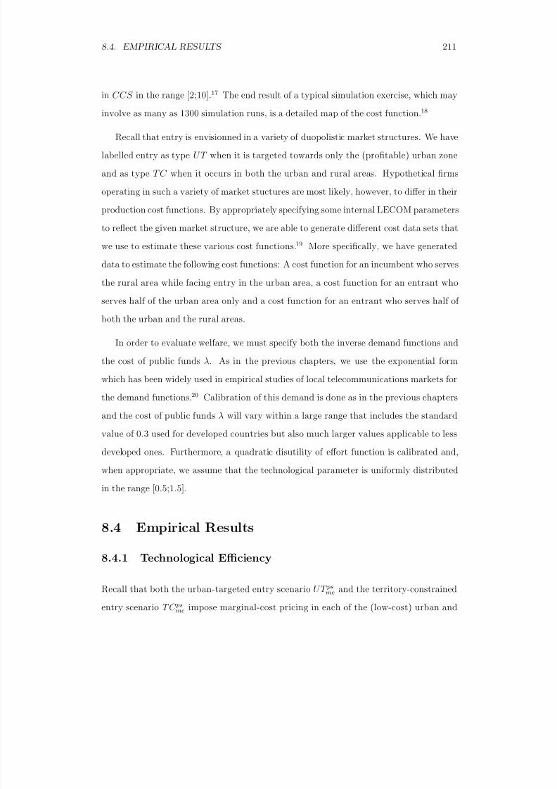
8/18/2019 Gasmi Cost Proxy Models
http://slidepdf.com/reader/full/gasmi-cost-proxy-models 211/318
8.4. EMPIRICAL RESULTS 211
in CCS in the range [2;10].17 The end result of a typical simulation exercise, which may
involve as many as 1300 simulation runs, is a detailed map of the cost function.18
Recall that entry is envisionned in a variety of duopolistic market structures. We have
labelled entry as type U T when it is targeted towards only the (profitable) urban zone
and as type T C when it occurs in both the urban and rural areas. Hypothetical firms
operating in such a variety of market stuctures are most likely, however, to differ in their
production cost functions. By appropriately specifying some internal LECOM parameters
to reflect the given market structure, we are able to generate different cost data sets thatwe use to estimate these various cost functions.19 More specifically, we have generated
data to estimate the following cost functions: A cost function for an incumbent who serves
the rural area while facing entry in the urban area, a cost function for an entrant who
serves half of the urban area only and a cost function for an entrant who serves half of
both the urban and the rural areas.
In order to evaluate welfare, we must specify both the inverse demand functions and
the cost of public funds λ. As in the previous chapters, we use the exponential form
which has been widely used in empirical studies of local telecommunications markets for
the demand functions.20 Calibration of this demand is done as in the previous chapters
and the cost of public funds λ will vary within a large range that includes the standard
value of 0.3 used for developed countries but also much larger values applicable to less
developed ones. Furthermore, a quadratic disutility of effort function is calibrated and,
when appropriate, we assume that the technological parameter is uniformly distributed
in the range [0.5;1.5].
8.4 Empirical Results
8.4.1 Technological Efficiency
Recall that both the urban-targeted entry scenario UT psmc and the territory-constrained
entry scenario T C psmc impose marginal-cost pricing in each of the (low-cost) urban and
8/18/2019 Gasmi Cost Proxy Models
http://slidepdf.com/reader/full/gasmi-cost-proxy-models 212/318
212 CHAPTER 8. UNIVERSAL SERVICE
(high-cost) rural areas. Clearly then the universal service obligation to serve both areas
at the same price is violated. Nonetheless, a comparison of these two alternatives willprovide us with useful information on their relative merits on pure technological efficiency
grounds.
Because they both rely on costly public funds to finance the deficit, entry scenarios
U T psmc and T C ps
mc see their social welfare deteriorate with increasing values of the cost
of public funds λ. A closer examination of the data shows that these two scenarios
are quite close, with the urban-targeted scenario U T
ps
ms slightly dominating the territory-constrained scenario T C ps
mc.21 Figure 8.2 visualizes the situation. The slight improvement
of the performance of the urban-targeted scenario relative to the territory-constrained
scenario as λ increases shown in the figure may be explained by the relative size of the
deficit which is found to be somewhat larger for T C psmc than for U T ps
mc. To summarize,
we can say that under complete information, marginal-cost pricing and access to public
subsidies to finance the firms’ deficits, social welfare achieved under the urban-targeted
entry scenario UT psmc is slightly higher to that achieved under the territory-constrained
entry scenario T C psmc with the difference getting larger for greater values of the cost of
public funds.
W
λ
UT psmc
T C ps
mc
Figure 8.2: U T vs. T C under marginal-cost pricing
8/18/2019 Gasmi Cost Proxy Models
http://slidepdf.com/reader/full/gasmi-cost-proxy-models 213/318
8.4. EMPIRICAL RESULTS 213
Note, however, that under marginal-cost pricing, both scenarios fail to satisfy the
budget balance constraint, while the U T scenario also fails to satisfy the universal serviceobligation. In the remainder of this chapter we will consider alternative versions of these
scenarios that satisfy both constraints.
8.4.2 Universal Service Obligation and Budget Balance
Let us now examine the results for the competitive solutions that satisfy both the universal
service obligation and the balanced-budget constraint.22
Scenario U T psac assumes that the
entrant captures half of the urban area and that the incumbent serves the other half
as well as the whole rural area. Under this scenario, the incumbent has to match the
entrant’s (average-cost) price in the urban area and apply that same price in the rural
area because of the obligation to offer service at affordable prices. This implies a deficit
which is financed from external funds provided by public subsidies.23 In contrast, under
scenario T C ac which assumes that the whole territory is divided in half, the universal
service obligation is financed internally through urban-to-rural cross-subsidies imposed
by budget balance in each half of the territory. Consequently, while the performance of
T C ac is independent of λ, socially costly public subsidies make social welfare achieved
under scenario UT psac decrease with increasing values of λ. Figure 8.3 below shows the
critical value of the cost of public funds λ∗ beyond which T C ac outperforms U T psac . This
parameter is found to satisfy 0.1 < λ∗ < 0.2.

8/18/2019 Gasmi Cost Proxy Models
http://slidepdf.com/reader/full/gasmi-cost-proxy-models 214/318
214 CHAPTER 8. UNIVERSAL SERVICE
W
λ∗ λ
U T ps
ac
0.1 0.2
T C ac
Figure 8.3: U T vs. T C under average-cost pricing
We can then state that under complete information and a balanced-budget constraint,
for any value of the cost of public funds λ > λ∗, the territory-constrained entry scenario
T C ac that allows for urban-to-rural cross-subsidies achieves a strictly higher level of social
welfare than the urban-targeted entry scenario U T psac in which public subsidies are used
to finance the incumbent’s deficit due to uniform pricing.
In view of the finding of the previous subsection (that UT slightly dominates T C ),
the current result has some interesting policy implications. Since our default value of λ
for highly developed countries is equal to 0.3, it suggests that the territory constrained
solution can be expected to yield higher expected social welfare in both developed and
developing countries when a uniform price is imposed in both urban and rural regions.
Our analysis suggests that even highly efficient public funds transfer systems may impose
a social cost that is greater than the dead-weight losses associated with uniform pricing
regimes, at least for the demand elasticities that we assume.
To conclude this subsection we note that we have obtained an additional piece of
information. Indeed, because scenario T C ac relies on transfers internal to the firm whereas
U T psac uses public funds to finance universal service, the critical value λ∗ provides us with an
evaluation of the social cost associated with the distortions created by the cross-subsidies
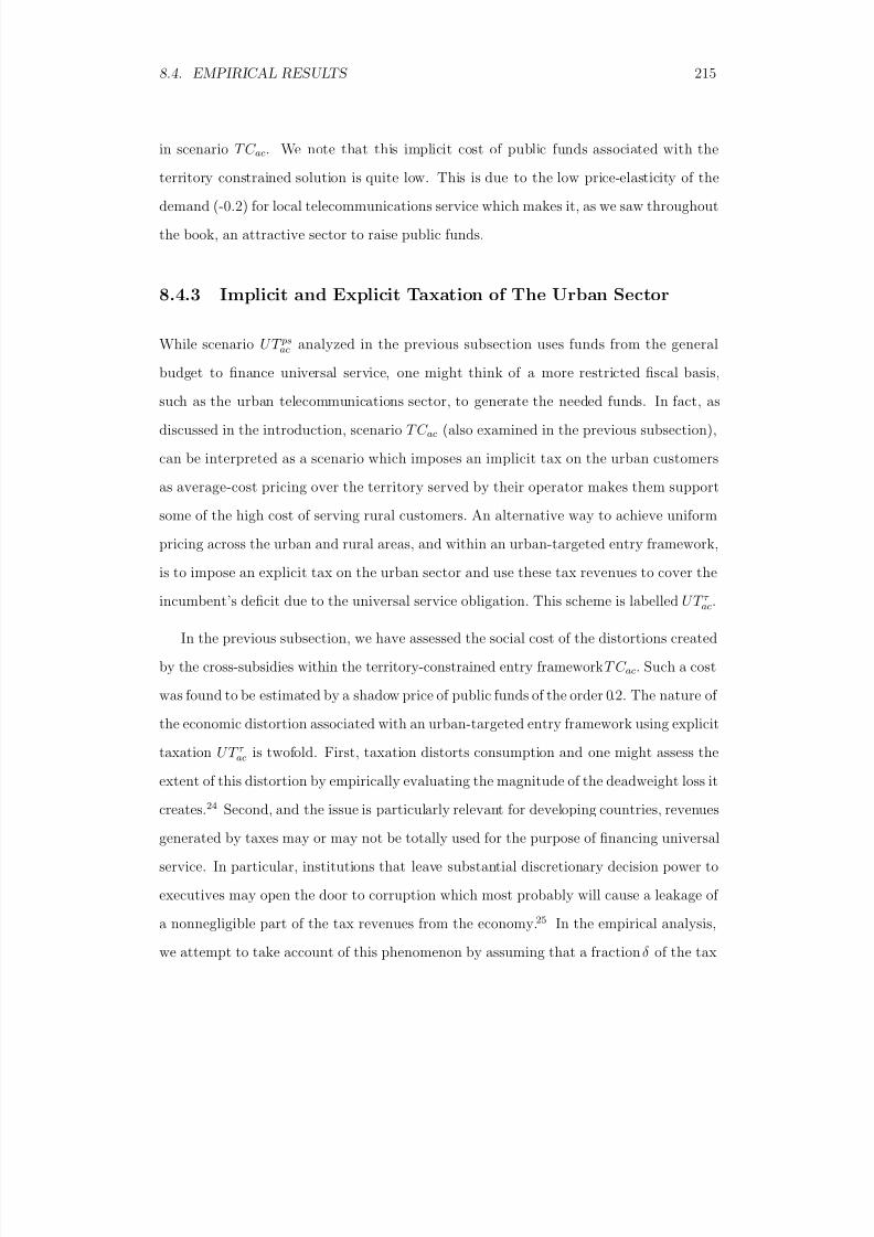
8/18/2019 Gasmi Cost Proxy Models
http://slidepdf.com/reader/full/gasmi-cost-proxy-models 215/318
8.4. EMPIRICAL RESULTS 215
in scenario T C ac. We note that this implicit cost of public funds associated with the
territory constrained solution is quite low. This is due to the low price-elasticity of thedemand (-0.2) for local telecommunications service which makes it, as we saw throughout
the book, an attractive sector to raise public funds.
8.4.3 Implicit and Explicit Taxation of The Urban Sector
While scenario U T psac analyzed in the previous subsection uses funds from the general
budget to finance universal service, one might think of a more restricted fiscal basis,
such as the urban telecommunications sector, to generate the needed funds. In fact, as
discussed in the introduction, scenario T C ac (also examined in the previous subsection),
can be interpreted as a scenario which imposes an implicit tax on the urban customers
as average-cost pricing over the territory served by their operator makes them support
some of the high cost of serving rural customers. An alternative way to achieve uniform
pricing across the urban and rural areas, and within an urban-targeted entry framework,
is to impose an explicit tax on the urban sector and use these tax revenues to cover the
incumbent’s deficit due to the universal service obligation. This scheme is labelled UT τ ac.
In the previous subsection, we have assessed the social cost of the distortions created
by the cross-subsidies within the territory-constrained entry framework T C ac. Such a cost
was found to be estimated by a shadow price of public funds of the order 0.2. The nature of
the economic distortion associated with an urban-targeted entry framework using explicittaxation UT τ
ac is twofold. First, taxation distorts consumption and one might assess the
extent of this distortion by empirically evaluating the magnitude of the deadweight loss it
creates.24 Second, and the issue is particularly relevant for developing countries, revenues
generated by taxes may or may not be totally used for the purpose of financing universal
service. In particular, institutions that leave substantial discretionary decision power to
executives may open the door to corruption which most probably will cause a leakage of
a nonnegligible part of the tax revenues from the economy.25 In the empirical analysis,
we attempt to take account of this phenomenon by assuming that a fraction δ of the tax
8/18/2019 Gasmi Cost Proxy Models
http://slidepdf.com/reader/full/gasmi-cost-proxy-models 216/318
216 CHAPTER 8. UNIVERSAL SERVICE
revenues, which we let vary from 0.5 to 1 by increments of 0.1, is actually used to finance
universal service and, therefore, a fraction 1 − δ of these public funds is embezzled byprivate interests.
We observe that in the no corruption state, i.e., when the totality of tax revenues is
indeed used to finance universal service (δ = 1), the performance of scenario U T τ ac should
be as good as that of scenario T C ac in the absence of a technological advantage to the T C .
Under these circumstances, both of these scenarios can be expected to create distortions
of the same magnitude, i.e., corresponding to a shadow price of public funds λ
∗
closeto 0.2. We have argued above that the cost of public funds is generally considered to
be greater than λ∗ in developing countries and therefore we would expect that U T τ ac is
dominated by T C ac in such countries. Clearly, decreasing values of δ would increase the
social cost of the distortions associated with explicit taxation and hence would favor the
territory-constrained entry scenario T C ac. We have evaluated scenario U T τ ac for each of
the 6 values of δ and calculated the corresponding values of the implicit cost of public
funds λ. Table 8.1 below exhibits the results which, as expected, show that, as the portion
of tax revenues actually used to finance universal service (δ ) increases, the dead-weight
loss due to taxation decreases and this financing tool becomes more and more attractive
as reflected in a decreasing implicit cost of public funds.
Table 8.1Funding of universal service
through explicit taxation(Implicit cost of public funds)
Value of δ λ0.5 1.350.6 0.940.7 0.640.8 0.430.9 0.261.0 0.13
8/18/2019 Gasmi Cost Proxy Models
http://slidepdf.com/reader/full/gasmi-cost-proxy-models 217/318
8.4. EMPIRICAL RESULTS 217
8.4.4 Impact of Incomplete Information
So far, even though competition was motivated by informational reasons, the analysis
has been conducted under complete information and we have presumed that all types
of competition eliminate information rents. However, given the particular importance of
asymmetric information in both developed and developing countries, it is interesting to
examine further how it affects our comparisons.26 We now investigate further the desir-
ability of cross-subsidies as a means of financing universal service when the (social) cost
of incomplete information is taken into account. A U T -type entry scenario is considered
once more but we now assume that the entrant in the urban area has the most efficient
technology and, as in scenario U T psac , we impose affordability through complete informa-
tion regulation. This scenario, labelled UT psac, is compared with a T C -type scenario in
which the incumbent and the entrant serve half of the whole territory and are regulated
under incomplete information with price cap (T C P C ).27 Because the performance of
U T psac decreases with λ, we find the critical values of this parameter λ∗∗, which is be-
tween 0.4 and 0.5, beyond which the T C -type scenario T C P C dominates it despite the
incomplete information (see Figure 8.4 below).28
The immediate implication of this result is that, if taxation of the urban telecommu-
nications is not feasible and one must only rely on the general budget to fund universal
service, as long as the cost of public funds is sufficiently high (which is the case in LDCs),
a T C -type solution is to be preferred to a UT -type, even if the informational costs of
regulation are accounted for in the T C solution.
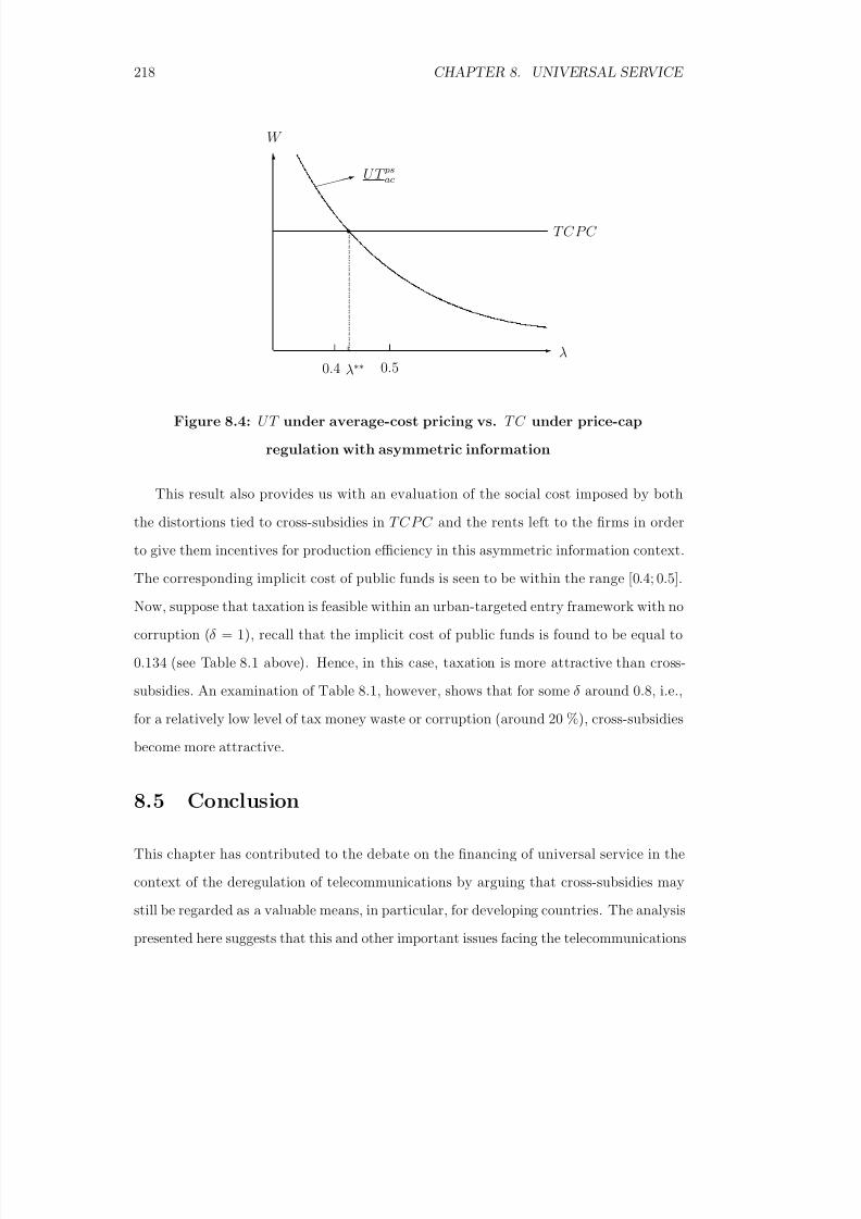
8/18/2019 Gasmi Cost Proxy Models
http://slidepdf.com/reader/full/gasmi-cost-proxy-models 218/318
218 CHAPTER 8. UNIVERSAL SERVICE
W
λ∗∗ λ
U T ps
ac
0.4 0.5
T C P C
Figure 8.4: U T under average-cost pricing vs. T C under price-cap
regulation with asymmetric information
This result also provides us with an evaluation of the social cost imposed by both
the distortions tied to cross-subsidies in T C P C and the rents left to the firms in order
to give them incentives for production efficiency in this asymmetric information context.
The corresponding implicit cost of public funds is seen to be within the range [0 .4; 0.5].
Now, suppose that taxation is feasible within an urban-targeted entry framework with no
corruption (δ = 1), recall that the implicit cost of public funds is found to be equal to
0.134 (see Table 8.1 above). Hence, in this case, taxation is more attractive than cross-
subsidies. An examination of Table 8.1, however, shows that for some δ around 0.8, i.e.,
for a relatively low level of tax money waste or corruption (around 20 %), cross-subsidies
become more attractive.
8.5 Conclusion
This chapter has contributed to the debate on the financing of universal service in the
context of the deregulation of telecommunications by arguing that cross-subsidies may
still be regarded as a valuable means, in particular, for developing countries. The analysis
presented here suggests that this and other important issues facing the telecommunications
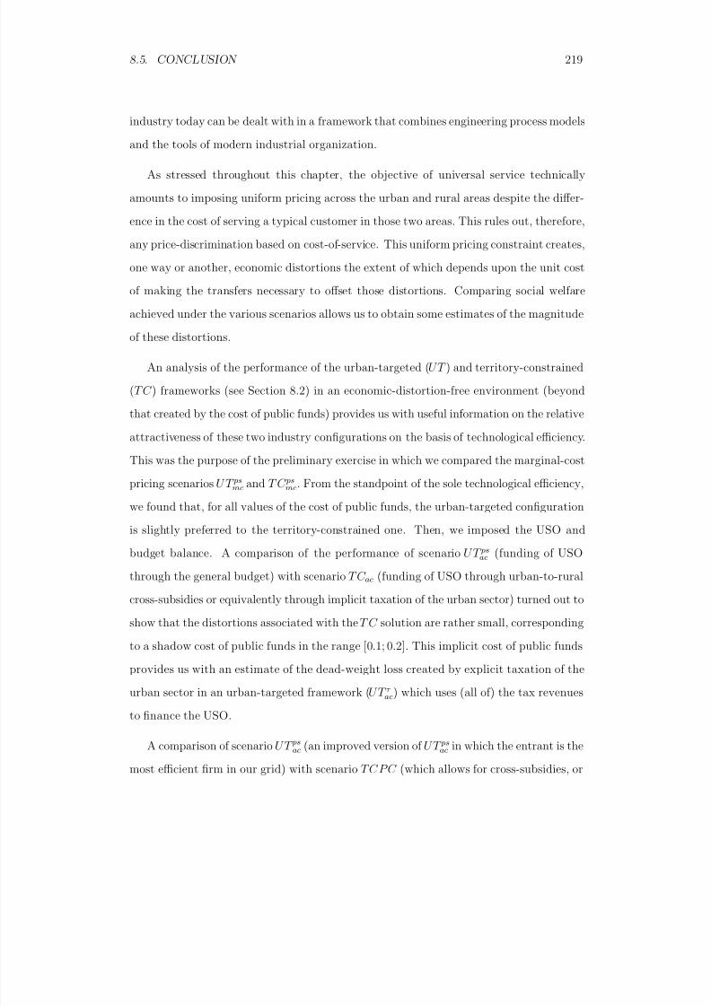
8/18/2019 Gasmi Cost Proxy Models
http://slidepdf.com/reader/full/gasmi-cost-proxy-models 219/318
8.5. CONCLUSION 219
industry today can be dealt with in a framework that combines engineering process models
and the tools of modern industrial organization.
As stressed throughout this chapter, the objective of universal service technically
amounts to imposing uniform pricing across the urban and rural areas despite the differ-
ence in the cost of serving a typical customer in those two areas. This rules out, therefore,
any price-discrimination based on cost-of-service. This uniform pricing constraint creates,
one way or another, economic distortions the extent of which depends upon the unit cost
of making the transfers necessary to offset those distortions. Comparing social welfareachieved under the various scenarios allows us to obtain some estimates of the magnitude
of these distortions.
An analysis of the performance of the urban-targeted (UT ) and territory-constrained
(T C ) frameworks (see Section 8.2) in an economic-distortion-free environment (beyond
that created by the cost of public funds) provides us with useful information on the relative
attractiveness of these two industry configurations on the basis of technological efficiency.
This was the purpose of the preliminary exercise in which we compared the marginal-cost
pricing scenarios U T psmc and T C ps
mc. From the standpoint of the sole technological efficiency,
we found that, for all values of the cost of public funds, the urban-targeted configuration
is slightly preferred to the territory-constrained one. Then, we imposed the USO and
budget balance. A comparison of the performance of scenario U T psac (funding of USO
through the general budget) with scenario T C ac (funding of USO through urban-to-rural
cross-subsidies or equivalently through implicit taxation of the urban sector) turned out to
show that the distortions associated with the T C solution are rather small, corresponding
to a shadow cost of public funds in the range [0 .1; 0.2]. This implicit cost of public funds
provides us with an estimate of the dead-weight loss created by explicit taxation of the
urban sector in an urban-targeted framework (U T τ ac) which uses (all of) the tax revenues
to finance the USO.
A comparison of scenario U T psac (an improved version of U T ps
ac in which the entrant is the
most efficient firm in our grid) with scenario T C P C (which allows for cross-subsidies, or
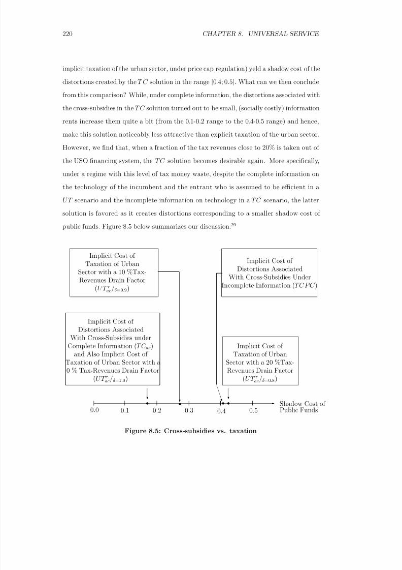
8/18/2019 Gasmi Cost Proxy Models
http://slidepdf.com/reader/full/gasmi-cost-proxy-models 220/318
220 CHAPTER 8. UNIVERSAL SERVICE
implicit taxation of the urban sector, under price cap regulation) yeld a shadow cost of the
distortions created by the T C solution in the range [0.4; 0.5]. What can we then concludefrom this comparison? While, under complete information, the distortions associated with
the cross-subsidies in the T C solution turned out to be small, (socially costly) information
rents increase them quite a bit (from the 0.1-0.2 range to the 0.4-0.5 range) and hence,
make this solution noticeably less attractive than explicit taxation of the urban sector.
However, we find that, when a fraction of the tax revenues close to 20% is taken out of
the USO financing system, the T C solution becomes desirable again. More specifically,
under a regime with this level of tax money waste, despite the complete information on
the technology of the incumbent and the entrant who is assumed to be efficient in a
U T scenario and the incomplete information on technology in a T C scenario, the latter
solution is favored as it creates distortions corresponding to a smaller shadow cost of
public funds. Figure 8.5 below summarizes our discussion.29
0.0 0.1 0.2 0.3 0.4 0.5Shadow Cost of Public Funds
Implicit Cost of Distortions Associated
With Cross-Subsidies UnderIncomplete Information (T C P C )
Implicit Cost of Taxation of Urban
Sector with a 10 %Tax-Revenues Drain Factor
(UT τ ac/δ=0.9)
Implicit Cost of Taxation of Urban
Sector with a 20 %Tax-Revenues Drain Factor
(UT τ ac/δ=0.8)
Implicit Cost of Distortions Associated
With Cross-Subsidies underComplete Information (T C ac)
and Also Implicit Cost of Taxation of Urban Sector with a0 % Tax-Revenues Drain Factor
(U T τ ac/δ=1.0)
Figure 8.5: Cross-subsidies vs. taxation
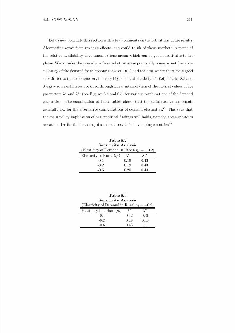
8/18/2019 Gasmi Cost Proxy Models
http://slidepdf.com/reader/full/gasmi-cost-proxy-models 221/318
8.5. CONCLUSION 221
Let us now conclude this section with a few comments on the robustness of the results.
Abstracting away from revenue effects, one could think of those markets in terms of the relative availability of communications means which can be good substitutes to the
phone. We consider the case where those substitutes are practically non-existent (very low
elasticity of the demand for telephone usage of −0.1) and the case where there exist good
substitutes to the telephone service (very high demand elasticity of −0.6). Tables 8.3 and
8.4 give some estimates obtained through linear interpolation of the critical values of the
parameters λ∗ and λ∗∗ (see Figures 8.4 and 8.5) for various combinations of the demand
elasticities. The examination of these tables shows that the estimated values remain
generally low for the alternative configurations of demand elasticities.30 This says that
the main policy implication of our empirical findings still holds, namely, cross-subsidies
are attractive for the financing of universal service in developing countries.31
Table 8.2
Sensitivity Analysis(Elasticity of Demand in Urban η1 = −0.2)
Elasticity in Rural (η2) λ∗ λ∗∗
-0.1 0.19 0.43-0.2 0.19 0.43-0.6 0.20 0.43
Table 8.3Sensitivity Analysis
(Elasticity of Demand in Rural η2 = −0.2)
Elasticity in Urban (η1) λ∗ λ∗∗
-0.1 0.12 0.31-0.2 0.19 0.43-0.6 0.43 1.1

8/18/2019 Gasmi Cost Proxy Models
http://slidepdf.com/reader/full/gasmi-cost-proxy-models 222/318
222 NOTES
Notes
1Competition between those incumbents and entrants has by now been organized.
2Another option under consideration in the United States consists of simultaneously
introducing competition in low cost areas and organizing universal service auctions for the
subsidies needed in high cost areas to obtain affordable prices. Note, however, that the
good performance of such auctions, which might turn out to be quite complex, requires
a great deal of regulatory expertise and depends crucially on how genuinely competitive
the participants’ behavior is.
3In the case of duopoly, which will be the main focus of our analysis, q ij will designate
the output of firm j in area i (see below).
4Although the focus of this chapter is to compare the performance of alternative com-
petitive scenarios, for clarity of exposition it is useful to start from a monopoly framework.
At this point, the reader might find it useful to take a glance at Figure 1 below which
visualizes the generic market structures that we consider in the empirical analysis.
5Since, in our analysis, the urban and rural subscribers populations N 1 and N 2 are
held constant, they will be kept as arguments of the various cost functions considered
only when necessary.
6Unless indicated otherwise, we assume that the entrant has the same technological
efficiency parameter β as the incumbent.
7For reference, the top of Figure 8.1 shows a monopolistic situation.
8Optimal effort equates marginal disutility and marginal cost saving.
9Note that in the urban sector, it is the marginal cost of the entrant (firm 2) that
imposes the price.
10This interpretation of universal service may be oversimplifying to some extent the

8/18/2019 Gasmi Cost Proxy Models
http://slidepdf.com/reader/full/gasmi-cost-proxy-models 223/318
NOTES 223
policy initiatives in both developed and developing countries. For example, in the United
States, universal service is currently interpreted as the right to purchase a set of services(voice grade plus access to advanced services) at a benchmark price which does not nec-
essarily equal the price of the low-cost urban area. However, in many countries universal
service entails uniform pricing.
11In this chapter, we designate by “balanced-budget” regulation a regulation in which
the firm’s participation constraint is binding without transfers from the regulator. Such
a constraint, recall, means that revenues must recover production costs as well as the
disutility of effort.
12In fact, our empirical analysis shows that in this case the (residual) average cost
function is consistently above the inverse demand function.
13The subscript “ac” indicates that average cost pricing is used.
14
An optimization is needed when (8.17) has several solutions in q 1.
15Excise taxes on telecommunications services have been imposed in the United States
at the federal level and by various state and local authorities. In the implementation of
the 1996 Telecommunications Act, a universal service fund was funded through surcharges
on revenues of all telecommunications carriers as defined in the Act.
16This price cap regulatory mechanism is discussed in great detail in Chapters 4 and 7.
17Note that here we use a larger range of usage (up to 10 CCS instead of 5.5 CCS ) than
in the previous chapters to account for the higher value of service (than under monopoly)
that competition is supposed to bring to subscribers.
18For all of the simulations, we take as a base case a local exchange market consisting
of 50 000 urban subscribers and 2 000 rural subscribers in a total territory covering about
207 square miles.
19For entry scenario U T we simulate the cost functions of both the incumbent and

8/18/2019 Gasmi Cost Proxy Models
http://slidepdf.com/reader/full/gasmi-cost-proxy-models 224/318
224 NOTES
the (urban) entrant by adjusting the size of the city and its population to represent
the territory served by each. The territory served by the entrant represents one half of the territory formerly served by the monopolist with one half of the monopolist’s urban
customers (and hence the same urban population density). The territory served by the
incumbent represents the entire area urban and rural territory of the former monopolist,
with one half of the urban area and one half of the urban population removed. For the
T C entry scenario, we assume that each duopolist served a territory having one half of
the area (urban and rural) and one half of the population (urban and rural) of the former
monopolist. All of these simulations were implemented by appropriately modifying the
input files “populatn.dat” and “rectangl.dat” as explained in the LECOM documentation
(Gabel and Kennet, 1991).
20In Section 8.5, we examine the sensitivity of our results to the demand elasticities.
21See Appendix A at the end of the book for the raw data obtained in this empirical
analysis.
22In fact, from now on we will consider only scenarios that satisfy the universal service
obligation, i.e., the obligation to serve the urban and rural areas at a uniform price.
23As mentioned in Section 2, we have found that a U T scenario in which the incumbent
matches the entrant’s price in the urban market and sets price equal to average residual
cost in the rural market is not viable, i.e., there is no rural price that allows the incumbent
to break even.
24We approximate this distortion in the usual fashion, namely, as the area of the triangle
formed by the demand and supply curves, that measures the “excess burden” of the tax,
i.e., the amount that consumers and producers are willing to pay to avoid this tax.
25While the phenomenon of corruption is not peculiar to developing countries, its quan-
titative importance (e.g., in terms of the percentage of GNP concerned by the phe-
nomenon), its generalization to most of the sectors of the economy and the fact that

8/18/2019 Gasmi Cost Proxy Models
http://slidepdf.com/reader/full/gasmi-cost-proxy-models 225/318
NOTES 225
it is chronic, make it a serious impediment to their economic and social development.
26In particular, the fact that there are no satisfactory accounting and auditing proce-
dures in developing countries appropriately exacerbates the issue of asymmetric informa-
tion.
27We perform this comparison to take account of the fact that the U T solution is likely
to be more competitive. It should make the most favorable case for the U T -type scenario
in the relevant range of λ and hence would reinforce the case for cross-subsidies if the
T C solution turns out to be still the best. Nevertheless, note that we require a rather
efficient regulation in the T C solution (optimal price cap) which might not be feasible in
developing countries.
28Note that because UT psac dominates UT ps
ac in the relevant range of λ and T C ac dom-
inates T C P C , we find, as expected, λ∗∗ > λ∗. Furthermore, note that a comparison of
T C P C with UT psac rather than U T ps
ac yields a smaller critical value of λ (between 0.3 and
0.4).
29In this figure we designate by “tax-revenues drain factor” the proportion of tax rev-
enues which is taken away from the universal service funding system.
30Note that the case of a very high elasticity in the urban market leads to a somewhat
higher value of λ∗∗, i.e., a higher social cost of asymmetric information.
31Gasmi et al (2001) find an even more favorable case for cross-subsidies in densely
populated developing countries.

8/18/2019 Gasmi Cost Proxy Models
http://slidepdf.com/reader/full/gasmi-cost-proxy-models 226/318
226 NOTES
8/18/2019 Gasmi Cost Proxy Models
http://slidepdf.com/reader/full/gasmi-cost-proxy-models 227/318
Chapter 9
Strategic Cross-Subsidies and
Vertical Integration
9.1 Introduction
When competition is introduced in markets for services using an infrastructure, an im-
portant structural decision that needs to be made concerns the vertical disintegration of
the incumbent firm which provides both the infrastructure and the services. Preventing
the owner of the infrastructure to compete in services, as Judge Greene decided in the
AT&T case, may destroy potential economies of scope, create more transaction costs,
but eliminates most incentives for favoritism due to the incumbent’s internal use of the
infrastructure.
In Europe, the liberalization reforms have maintained the vertical integration of in-cumbent operators accompanied with a requirement of accounting separation between
services and infrastructure activities. In the United States, the FCC has issued a series
of rulemakings, known as the Computer Inquires, which have progressively weakened the
separation requirements by moving from a regime of structural safeguards to various forms
of accounting safeguards.1 This chapter provides an empirical evaluation of these types of
policies as a means to introduce competition in services markets. In particular, we exam-
ine the impact that the cross-subsidies allowed by vertical integration of the incumbent
may have on the competitive process in these markets.
227
8/18/2019 Gasmi Cost Proxy Models
http://slidepdf.com/reader/full/gasmi-cost-proxy-models 228/318
228CHAPTER 9. STRATEGIC CROSS-SUBSIDIES AND VERTICAL INTEGRATION
We consider a situation where two segments use a common (telecommunications)
infrastructure. We envision the introduction of competition in one segment while theother segment is serviced by an incumbent regulated firm. In Section 9.2, we seek to
model the phenomenon of manipulation, via cross-subsidies, which could result from the
accounting procedure of allocating common costs between the two services.
Even with accounting separation, manipulation of moral hazard variables such as effort
levels creates cross-subsidies when the regulated segment is subject to cost-plus regulation
while the firm is residual claimant of its costs in the competitive segment. Section 9.3shows how the size of such cross-subsidies varies with the power of incentives in the
regulated sector while Section 9.4 studies how these cross-subsidies may affect entry.
Section 9.5 presents some empirical results based on a LECOM simulation of costs
for the case in which potential cross-subsidies may exist between the markets for basic
(switched) telephone service and enhanced services supplied to a (non-switched) compet-
itive sector using leased lines. Section 9.6 contains some concluding remarks.
9.2 Size of Cross-Subsidies Due to Allocation of Com-mon Costs
Consider a service territory composed of two markets. Market 1 is assumed to be open
to competitive entry and market 2 is assumed to have the technological characteristics
of a natural monopoly. An incumbent firm operates in both of these markets with a
technology described by a cost function C which can be represented as follows:
C (β, e0, e1, e2, q 1, q 2) = C 1(β, e1, q 1, q 2) + C 2(β, e2, q 1, q 2) + C 0(β, e0, q 1, q 2) (9.1)
where
- C 1(·), C 2(·) and C 0(·) are functions that represent, respectively, incremental costs of
the activities on markets 1 and 2 and costs that are common to the two activities.
8/18/2019 Gasmi Cost Proxy Models
http://slidepdf.com/reader/full/gasmi-cost-proxy-models 229/318
9.2. SIZE OF CROSS-SUBSIDIES DUE TO ALLOCATION OF COMMON COSTS 229
- β is a technological parameter.
- eo, e1 and e2 are efforts that reduce the respective components of the total cost.
- q 1 and q 2 are output levels in markets 1 and 2.
Equation (9.1) assumes a particular decomposition of the cost function C in which
both the effort variables e0, e1 and e2 and the output variables q 1 and q 2 can be assigned
to the functions C 0, C 1 and C 2 respectively. An important assumption in this decompo-
sition is that the effort levels e0, e1 and e2 can be individually applied to the component
cost functions. This assumption is carried over to the function that gives the aggregate
disutility generated by these effort levels for the incumbent. More specifically, we assume
that this disutility of effort function is expressed as
ψ(β, e0, e1, e2, q 1, q 2) = ψ1(β, e1, q 1) + ψ2(β, e2, q 2) + ψ0(β, e0). (9.2)
This approach is in contrast to an alternative approach in which effort is viewed as a“public” input which is applied equally to all of the firm’s activities. As explained in
more detail in Section 9.5, the latter approach is the one that we have adopted in previous
chapters, and it is the one that is consistent with our LECOM simulations of the total cost
function, where we use the price of labor as a proxy for aggregate effort. In the present
chapter, since we primarily deal with incremental cost functions, the interpretation of
effort as a “private” input to each activity is more appropriate.2
We also assume that the decomposition property holds for the stand-alone cost func-
tions corresponding to the two activities, SAC 1(.) and SAC 2(.), given by:
SAC 1(β, e0, e1, q 1) = C 1(β, e1, q 1, 0) + C 0(β, e0, q 1, 0) (9.3)
SAC 2(β, e0, e2, q 2) = C 2(β, e2, 0, q 2) + C 0(β, e0, 0, q 2). (9.4)
Let us initially focus on cross-subsidies that the firm could achieve through the al-
location of the common costs C 0(β, e0, q 1, q 2). Assume that the exogenous technological
8/18/2019 Gasmi Cost Proxy Models
http://slidepdf.com/reader/full/gasmi-cost-proxy-models 230/318
230CHAPTER 9. STRATEGIC CROSS-SUBSIDIES AND VERTICAL INTEGRATION
parameter β is known and that output and effort levels that affect the different cost com-
ponents are given. Furthermore, let δ ∈ [0, 1] represent a parameter that specifies the waycommon costs are allocated between the two activities. Specifically, δ represents the pro-
portion of the common costs which is allocated by the firm to the potentially competitive
segment (market 1). Omitting the arguments for simplicity, total cost of the firm can be
written as
C = C 1 + C 2 + C 0 = [C 1 + δC 0] + [C 2 + (1 − δ )C 0]. (9.5)
Equation (9.5) merely shows the decomposition of the total cost C into two parts corre-
sponding to the total costs associated with each of the two activities.
A straightforward way of assessing the potential that the firm has for subsidization of
activity 1 by activity 2 via the allocation of common costs, is by evaluating the relative
importance of these common costs. Clearly segment 1 would benefit from the high-
est (cross-)subsidies when the common costs are totally allocated to segment 2. More
formally, let s(δ ) represent the total cost allocated by the vertically integrated firm to
segment 1, namely,
s(δ ) = C 1 + δC 0. (9.6)
This function increases with δ from s(0) = C 1 to s(1) = C 1 + C 0 (Figure 9.1 below
displays the function s). If the parameter δ is under the control of the firm, the function
s may be used as a basis for constructing some measures of the cost advantage that
the vertically integrated firm possesses over its potential competitors in the liberalized
sector. This advantage is due to the incumbent firm’s ability to subsidize activity 1 from
revenues earned in activity 2. This type of cross-subsidy may be particularly attractive
to the firm when the market for activity 1 is competitive while activity 2 is regulated by
a low-powered cost-based scheme.

8/18/2019 Gasmi Cost Proxy Models
http://slidepdf.com/reader/full/gasmi-cost-proxy-models 231/318
9.3. SIZE OF EFFORT ALLOCATION CROSS-SUBSIDIES 231
1
δ
C 1
0
s
C 1 + C 0
Figure 9.1: Size of cross-subsidies through allocation of common costs
9.3 Size of Effort Allocation Cross-Subsidies
When strict accounting rules are in place, cross-subsidization may still be possible for
an integrated firm through its control of the effort variables e0, e1 and e2. In order to
evaluate the size of these strategic cross-subsidies, let us examine more closely how the
incumbent firm sets these effort levels. We go back to the total cost function given in
Equation (9.1) above and assume that the scheme under which the incumbent is regulated
can be described by a cost-reimbursement rule. More specifically, we assume that the firm
bears some given fractions α1, α2 and α0 of the costs of activities 1 and 2 respectively
and of the costs common to these activities.3
To determine effort allocation between the two activities and common costs, the firm
minimizes
α1C 1(β, e1, q 1, q 2) + α2C 2(β, e2, q 1, q 2) + α0C 0(β, e0, q 1, q 2) + ψ(β, e0, e1, e2, q 1, q 2) (9.7)
where ψ is given in Equation (9.2) above. The first-order conditions of this problem are
∂ψ1
∂e1(β, e1, q 1) ≥ −α1
∂C 1∂e1
(β, e1, q 1, q 2) (9.8)
∂ψ2
∂e2(β, e2, q 2) ≥ −α2
∂C 2∂e2
(β, e2, q 1, q 2) (9.9)
∂ψ0
∂e0
(β, e0) ≥ −α0∂C 0∂e0
(β, e0, q 1, q 2) (9.10)
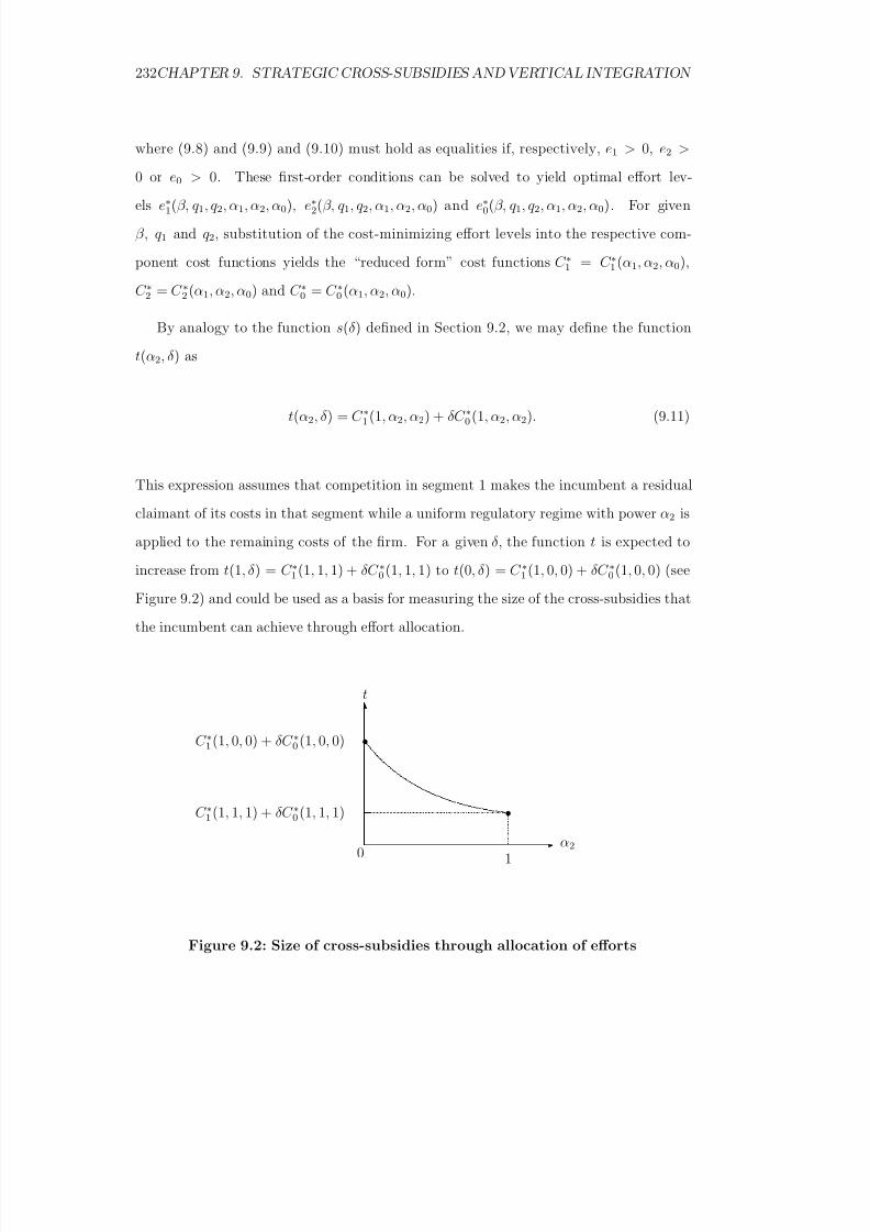
8/18/2019 Gasmi Cost Proxy Models
http://slidepdf.com/reader/full/gasmi-cost-proxy-models 232/318
232CHAPTER 9. STRATEGIC CROSS-SUBSIDIES AND VERTICAL INTEGRATION
where (9.8) and (9.9) and (9.10) must hold as equalities if, respectively, e1 > 0, e2 >
0 or e0 > 0. These first-order conditions can be solved to yield optimal effort lev-els e∗1(β, q 1, q 2, α1, α2, α0), e∗
2(β, q 1, q 2, α1, α2, α0) and e∗0(β, q 1, q 2, α1, α2, α0). For given
β , q 1 and q 2, substitution of the cost-minimizing effort levels into the respective com-
ponent cost functions yields the “reduced form” cost functions C ∗1 = C ∗1 (α1, α2, α0),
C ∗2 = C ∗2 (α1, α2, α0) and C ∗0 = C ∗0 (α1, α2, α0).
By analogy to the function s(δ ) defined in Section 9.2, we may define the function
t(α2, δ ) as
t(α2, δ ) = C ∗1 (1, α2, α2) + δC ∗0 (1, α2, α2). (9.11)
This expression assumes that competition in segment 1 makes the incumbent a residual
claimant of its costs in that segment while a uniform regulatory regime with power α2 is
applied to the remaining costs of the firm. For a given δ , the function t is expected to
increase from t(1, δ ) = C ∗1 (1, 1, 1) + δC ∗0 (1, 1, 1) to t(0, δ ) = C ∗1 (1, 0, 0) + δC ∗0 (1, 0, 0) (see
Figure 9.2) and could be used as a basis for measuring the size of the cross-subsidies that
the incumbent can achieve through effort allocation.
1
α20
C ∗1 (1, 0, 0) + δC ∗0 (1, 0, 0)
C ∗1 (1, 1, 1) + δC ∗0 (1, 1, 1)
t
Figure 9.2: Size of cross-subsidies through allocation of efforts

8/18/2019 Gasmi Cost Proxy Models
http://slidepdf.com/reader/full/gasmi-cost-proxy-models 233/318
9.4. STRATEGIC CROSS-SUBSIDIES THROUGH EFFORT... 233
9.4 Strategic Cross-Subsidies Through Effort Alloca-
tion Under Accounting Separation
Section 9.3 defined the range of potential strategic cross-subsidies in a measure that is
roughly comparable to the measure of the potential range for accounting cross-subsidies
defined in Section 9.2. In this section, we explore the possibility that strategic cross-
subsidies be used by an integrated firm to blockade entry when detailed accounting rules
are in place, which seek to prevent accounting cross-subsidization. To simplify the em-
pirical analysis that we present in a later section, we seek to identify separately the two
channels through which an integrated incumbent may interfere with entry. First, we con-
sider a setting where the incumbent does not have any technological cost advantage and
show how it can still have the ability to manipulate effort in order to undercut the entrant
through disutility of effort. Then, we consider the case where aggregate disutility of effort
is “neutral”, i.e., held constant, and analyze the conditions under which the allocation of
effort of the incumbent gives it a technological cost advantage.
9.4.1 The Cost of Effort Channel
Consider the situation where the incumbent (I ) faces competition in segment 1 but is a
cost-plus regulated monopoly in segment 2. We assume that strict accounting separation
holds between its two subsidiaries. We further assume that imputation of common costs
is defined on the basis of output, so that total allocated costs C 1 and C 2 of the two
subsidiaries are generically given by
C 1 = C 1(β, e1, q 1, q 2) + q 1
q 1 + q 2C 0(β, e0, q 1, q 2) (9.12)
C 2 = C 2(β, e2, q 1, q 2) + q 2
q 1 + q 2C 0(β, e0, q 1, q 2) (9.13)
Assume that a firm E considers entry into the liberalized segment market (market 1)
by relying on the same technology as the incumbent. Such an entrant, assumed to have

8/18/2019 Gasmi Cost Proxy Models
http://slidepdf.com/reader/full/gasmi-cost-proxy-models 234/318
234CHAPTER 9. STRATEGIC CROSS-SUBSIDIES AND VERTICAL INTEGRATION
“fair” access to the facilities that are common to the two segments, would have a total
allocated cost function given by
C E = C E (β, eE 1, q E 1, q I 2) + q E 1
(q I 1 + q E 1) + q I 2C 0(β, eI 0, (q I 1 + q E 1), q I 2) (9.14)
where C E is the incremental cost of the entering firm, eE 1 and q E 1 are its effort and output
levels respectively and eI 0, q I 1 and q I 2 are the incumbent’s (common) cost-reducing effort
and output levels in the competitive and regulated segments, respectively, once entry
has occurred. We assume that C E has the same functional form as C 1, the incumbent’s
incremental cost function in market 1.4
Since the entering firm uses the same technology as the incumbent and competition
takes place in segment 1, efforts are conditionally optimal, and one can assume that the
incumbent and the entrant share the market at the same level of output (q I 1 = q E 1). The
pecuniary costs of the incumbent are given by
C I = C 1(β, eI 1, q I 1, q I 2) + q I 1
(q I 1 + q E 1) + q I 2
C 0(β, eI 0, (q I 1 + q E 1), q I 2), (9.15)
where eI 1 is the incumbent’s (incremental) cost-reducing effort in the competitive segment.
If the incumbent matches the entrant’s price, these costs are the same as the entrant’s and
the incumbent must therefore match the entrant’s effort level in the competitive segment.
Under these conditions e∗I 1(q I 1) = e∗E 1(q E 1).
Despite the fact that there are no intrinsic technological cost advantages to the in-
cumbent, the latter might still have the ability to block entry. Indeed, one might well
have
ψE (β, e∗E 1, q E 1) ≤ ψ(β, e∗I 0, e∗I 1, e∗I 2(q I 2), q I 1, q I 2) (9.16)
yet
ψE (β, e∗E 1, q E 1) > ψ(β, e∗I 0, e∗I 1, eM inI 2 , q I 1, q I 2) (9.17)
where ψE is the disutility of effort function of the entrant (in the competitive segment),
e∗E 1 is the entrant’s optimizing value of e1, e∗I 0 and e∗I 2 are the incumbent’s optimizing
8/18/2019 Gasmi Cost Proxy Models
http://slidepdf.com/reader/full/gasmi-cost-proxy-models 235/318
9.4. STRATEGIC CROSS-SUBSIDIES THROUGH EFFORT... 235
values of e0 and e2, and eM in2 is the minimal effort level that the incumbent can exert in
reducing the corresponding cost component.
Inequalities (9.16) and (9.17) suggest that if the incumbent firm has its cost reimbursed
at a minimum level of effort in the regulated segment (incremental cost and common
costs), then it may have the ability to reduce its total disutility of effort to the point that
it is lower than the disutility of effort of the entrant. Hence, despite perfect accounting
separation, complemented by a fair access price to the regulated sector, the incumbent
can, by strategically manipulating effort levels, undercut an entrant, even if the latterhappens to possess a comparable or even somewhat superior technology.
If the entrant uses a significantly better technology (β E << β ) than the incumbent,
the analysis of strategic manipulation of effort levels would allow us to compute the cost
advantage it provides to the incumbent, but nothing general can be said about whether
or not entry can be blockaded by the incumbent.
9.4.2 The Cost of Production Channel
In the previous subsection, we have examined the possible ability that an incumbent
would have to blockade entry into a liberalized sector by manipulating effort levels to
the point of making its disutility of effort in the regulated sector lower than first-best
efficiency would dictate. A critical (perhaps too critical) role is played in this analysis by
the disutility of effort functions of the incumbent and the entrant. From the standpoint
of empirical analysis, this reliance on the properties of the disutility of effort functions is
problematical since they are inherently unobservable, and we obtain them solely through
calibration. Therefore, in the remainder of this section we consider a similar argument
(blockade of entry) which is based only on the cost functions that LECOM allows us to
estimate.
In the remainder of this subsection, we impose, on both the incumbent and the entrant,
a fixed level of disutility of effort ψ.5 We assume that the entrant and the incumbent have

8/18/2019 Gasmi Cost Proxy Models
http://slidepdf.com/reader/full/gasmi-cost-proxy-models 236/318
236CHAPTER 9. STRATEGIC CROSS-SUBSIDIES AND VERTICAL INTEGRATION
the same disutility of effort functions, so that disutility for the entrant can be expressed
as
ψE (β, eE 0, eE 1, q E 1) = ψ(β, eE 0, eE 1, 0, q E 1, 0). (9.18)
Consider an entering firm which uses its own facilities and allocates effort between in-
cremental and common costs. Hence, it would determine levels of e0 and e1 by minimizing
its stand-alone cost SAC E (see Equation (9.3)) subject to the constraint
ψ(β, eE 0, eE 1, 0, q E 1, 0) = ψ. (9.19)
The first-order conditions of this problem, given by Equation (9.19) and
∂C 0∂e0
∂ψ
∂e0
=
∂C 1∂e1
∂ψ
∂e1
, (9.20)
can be solved to yield optimal efforts e∗E 0(β, q E 1) and e∗E 1(β, q E 1) and a stand-alone cost
function for the entrant given by
C E (β, q E 1) ≡ C 1(β, e∗E 1(β, q E 1), q E 1, 0) + C 0(β, e∗E 0(β, q E 1), q E 1, 0). (9.21)
Moreover, substituting back these optimal efforts into the entrant’s disutility of effort
function yields the reduced form disutility of effort function
ψE (β, q E 1) ≡ ψ(β, e∗E 0(β, q E 1), e∗E 1(β, q E 1), 0, q E 1, 0). (9.22)
While the entrant exerts effort to reduce its incremental and common costs only, the in-
cumbent has to allocate it among the three components of its cost function. Furthermore,
the incumbent is subject to regulation which we assume is represented by a three-part
cost-reimbursement scheme with powers α1, α2 and α0 applied to the respective cost
components. The incumbent’s optimal choices of e1, e2 and e0 are therefore obtained by
minimizing total supported cost given by Equation (9.7) subject to the constraint
ψ(β, e0, e1, e2, q 1, q 2) = ψ. (9.23)
8/18/2019 Gasmi Cost Proxy Models
http://slidepdf.com/reader/full/gasmi-cost-proxy-models 237/318
9.5. EMPIRICAL RESULTS 237
First-order conditions to the incumbent’s effort allocation problem are given by
αi ∂C i∂ei
∂ψ
∂ei
=
α j ∂C j∂e j
∂ψ
∂e j
, (9.24)
i, j = 0, 1, 2, i = j and Equation (9.23). These conditions implicitly define optimal effort
functions e∗I 1(β, q I 1, q E 1, q I 2, α1, α2, α0, ψ), e∗I 2(β, q I 1, q E 1, q I 2, α1, α2, α0, ψ) and e∗I 0(β, q I 1, q E 1,
q I 2, α1, α2, α0, ψ). Assuming accounting separation and imputation of common costs ac-
cording to output as in the previous subsection, the cost function of the incumbent in
activity 1, C I (β, q I 1, q E 1, q I 2, α1, α2, α0, ψ), which is the relevant one to consider as far as
comparison with the entrant is concerned, is given by:
C 1(β, e∗I 1(β, q I 1, q E 1, q I 2, α1, α2, α0, ψ), q I 1, q I 2)
+ q I 1
q I 1 + q I 2C 0(β, e∗I 0(β, q I 1, q E 1, q I 2, α1, α2, α0, ψ), q I 1, q I 2). (9.25)
The two functions C E in Equation (9.21) and C I in Equation (9.25) can be compared.
For given values of the arguments, one can define the cost advantage of the incumbent (or
handicap of the entrant) as the difference between these two costs, ∆ ≡ (C E − C I ). Four
factors are at work in the determination of ∆: the (dis)economies of scope between the
two activities, the power of incentives of regulation, the common costs imputation rule and
the fact that the entrant firm has to allocate effort between only the two components of
its stand-alone cost whereas the incumbent has to allocate it among three components.6
It is worthwhile to note that the cost gap ∆ depends on the respective powers of the
incentive scheme. In the following section we will empirically analyze this dependence.
9.5 Empirical Results
9.5.1 Simulation of LECOM: Basic vs Enhanced Services
In previous chapters, we have used LECOM to simulate a telecommunications cost func-
tion in which outputs have been represented as traffic, measured in CCS per access line

8/18/2019 Gasmi Cost Proxy Models
http://slidepdf.com/reader/full/gasmi-cost-proxy-models 238/318
238CHAPTER 9. STRATEGIC CROSS-SUBSIDIES AND VERTICAL INTEGRATION
(see Chapters 6, 7 and 8) and access lines (see Chapter 5).7 In this chapter we again
consider cost as a function of the number of access lines, but we now separate access linesinto two distinct kinds, depending on the type of telecommunications service that they
provide. Basic switched services, primarily sold to residential and small business users
are essentially used for voice and low speed data traffic. High capacity leased lines (also
called private lines) are primarily used by larger business users for high speed data and
other enhanced services.
In both advanced and less developed countries, business and enhanced services havebeen open to competitive entry for many years, while the markets for residential switched
services have retained the characteristics of natural monopoly, even where entry has been
allowed or encouraged by the regulator. Thus, switched access lines are priced subject to
regulatory control in nearly all countries, while enhanced services are generally provided
in a highly competitive environment. The issues of cross-subsidization, which this chapter
seeks to investigate, are therefore relevant for these markets.
Using LECOM we are able to estimate the cost of providing both switched and non-
switched access lines. We assume a city of fixed size consisting of three zones, a central
business district, a mixed commercial and residential district, and a residential district.
We also assume that customer density progressively increases as we move from the resi-
dential to the mixed and to the business districts.8
LECOM allows the user to specify the proportion of non-switched access lines in each
region of the city. For the simulations, the percentage of private line customers varied
from 0% to 100% in increments of 20%. The total population of the city varied from
6000 to 100, 000 subscribers.9 Thus, by varying both the population of subscribers and
the percentage of non-switched lines, we define a grid of output values which we use to
simulate the total cost function of the integrated firm. The grid also includes a range of
values for the multipliers of the price of capital and labor P K and P L, which are supposed
to represent, respectively, the technology type β and effort e.10 In order to simulate the
stand-alone cost functions for both switched and non-switched access lines, we set the
8/18/2019 Gasmi Cost Proxy Models
http://slidepdf.com/reader/full/gasmi-cost-proxy-models 239/318
9.5. EMPIRICAL RESULTS 239
non-switched percentages equal to 0 and 1 respectively, and vary the total number of
access lines in a manner consistent with our first grid. This exercise allows us to createthe data which we use to estimate the cost functions C (β, e, q 1, q 2), C 1(β, e, q 1, q 2) and
C 2(β, e, q 1, q 2) which are described above.11,12
We next explain the techniques that allow us to estimate the stand-alone cost func-
tions defined in (9.1), (9.3) and (9.4) above through simulations of LECOM and how
we use these functions to derive the incremental and common cost functions. By letting
the variables P K (the multiplier for the price of capital, our proxy for the technologicalparameter β ), P L (the multiplier for the price of labor, our proxy for effort e), q 1 and q 2
(measures of levels of output in markets 1 and 2) vary within a grid, we obtain the cost
function C (β, e, q 1, q 2).13 This function represents the stand-alone cost of an integrated
firm (the incumbent) serving markets 1 and 2. Using the same grid and restricting the
outputs so that only q 1 > 0 and q 2 > 0, we estimate the cost functionsSAC 1(β, e, q 1)
andSAC 2(β, e, q 2) which represent the stand-alone costs of a non-integrated firm serv-
ing markets 1 and 2 respectively. We note that these stand-alone cost functions do
not correspond exactly to the theoretical stand-alone cost functions C (β, e0, e1, e2, q 1, q 2),
SAC 1(β, e0, e1, q 1) and SAC 2(β, e0, e2, q 2) since they do not allow the firm to assign dif-
ferent effort levels to different activities or markets.
Using these three basic LECOM-generated cost functions C ,SAC 1 andSAC 2 we
define the empirical counterparts of the incremental cost functions C 1 and C 2 and the
common cost function C 0 as follows:
C 1(β, e1, q 1, q 2) = C (β, e1, q 1, q 2) −SAC 2(β, e1, q 2) (9.26)
C 2(β, e2, q 1, q 2) = C (β, e2, q 1, q 2) −SAC 1(β, e2, q 1) (9.27)
C 0(β, e0, q 1, q 2) =SAC 1(β, e0, q 1) +SAC 2(β, e0, q 2) − C (β, e0, q 1, q 2). (9.28)
Substituting from (9.26) and (9.27) yields
C 0(β, e0, q 1, q 2) = C (β, e0, q 1, q 2) − C 1(β, e0, q 1, q 2) − C 2(β, e0, q 1, q 2). (9.29)
8/18/2019 Gasmi Cost Proxy Models
http://slidepdf.com/reader/full/gasmi-cost-proxy-models 240/318
240CHAPTER 9. STRATEGIC CROSS-SUBSIDIES AND VERTICAL INTEGRATION
Before discussing results on economies of scope between basic switched service and en-
hanced high capacity service, let us say a few more words on the theoretical interpretationof the above LECOM-simulated cost functions.
Our use of the LECOM input P L as a proxy for the firm’s effort level implies a
constraint on the way effort is allocated among the components of the cost function rep-
resented in Equation (9.1). For any 4-tuple (PK , PL , Q1, Q2), which is our proxy for
(β, e, q 1, q 2), a LECOM run searches for the network configuration and technological char-
acteristics (number of switches, location, types of switches, distribution and transportplant, etc.) that minimize the total cost. For each run, a common value of P L, repre-
senting a level of effort e, is used in both markets and for the common costs.14
Thus, the cost function C (β, e, q 1, q 2) that LECOM simulates represents the cost func-
tion for an integrated firm which is assumed to minimize the sum of its three components,
C 1(β, e1, q 1, q 2) + C 2(β, e2, q 1, q 2) + C 0(β, e0, q 1, q 2) (9.30)
subject to the constraint e0 = e1 = e2 ≡ e. Indeed, the solution to this minimization
problem yields a total cost function
C 1(β, e, q 1, q 2) + C 2(β, e, q 1, q 2) + C 0(β, e, q 1, q 2) (9.31)
which has C (β, e, q 1, q 2) as its empirical counterpart as can be verified using Equations
(9.26), (9.27) and (9.28).
Note that Equation (9.28) gives a direct indication of whether or not economies of scope
between basic switched service and enhanced service exist. Indeed, if these two services
are provided by two separate firms, each firm would have to support the corresponding
stand-alone cost and the total multifirm cost would then be equal to (SAC 1 +SAC 2).
A single firm offering both of these services would bear the total cost C . The difference
between these two costs, [(SAC 1+SAC 2]−C ], which represents the costs that are common
to the two services, indicates the presence of economies or diseconomies of scope. For
various combinations of outputs q 1 (number of non-switched access lines) and q 2 (number
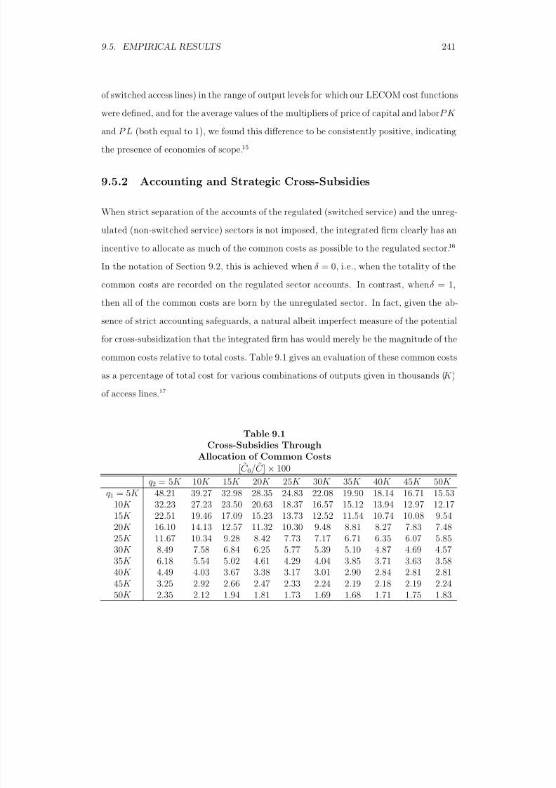
8/18/2019 Gasmi Cost Proxy Models
http://slidepdf.com/reader/full/gasmi-cost-proxy-models 241/318
9.5. EMPIRICAL RESULTS 241
of switched access lines) in the range of output levels for which our LECOM cost functions
were defined, and for the average values of the multipliers of price of capital and labor P K and P L (both equal to 1), we found this difference to be consistently positive, indicating
the presence of economies of scope.15
9.5.2 Accounting and Strategic Cross-Subsidies
When strict separation of the accounts of the regulated (switched service) and the unreg-
ulated (non-switched service) sectors is not imposed, the integrated firm clearly has an
incentive to allocate as much of the common costs as possible to the regulated sector.16
In the notation of Section 9.2, this is achieved when δ = 0, i.e., when the totality of the
common costs are recorded on the regulated sector accounts. In contrast, when δ = 1,
then all of the common costs are born by the unregulated sector. In fact, given the ab-
sence of strict accounting safeguards, a natural albeit imperfect measure of the potential
for cross-subsidization that the integrated firm has would merely be the magnitude of the
common costs relative to total costs. Table 9.1 gives an evaluation of these common costs
as a percentage of total cost for various combinations of outputs given in thousands (K )
of access lines.17
Table 9.1Cross-Subsidies Through
Allocation of Common Costs
[ C 0/C ] × 100
q 2 = 5K 10K 15K 20K 25K 30K 35K 40K 45K 50K q 1 = 5K 48.21 39.27 32.98 28.35 24.83 22.08 19.90 18.14 16.71 15.53
10K 32.23 27.23 23.50 20.63 18.37 16.57 15.12 13.94 12.97 12.1715K 22.51 19.46 17.09 15.23 13.73 12.52 11.54 10.74 10.08 9.5420K 16.10 14.13 12.57 11.32 10.30 9.48 8.81 8.27 7.83 7.4825K 11.67 10.34 9.28 8.42 7.73 7.17 6.71 6.35 6.07 5.8530K 8.49 7.58 6.84 6.25 5.77 5.39 5.10 4.87 4.69 4.5735K 6.18 5.54 5.02 4.61 4.29 4.04 3.85 3.71 3.63 3.5840K 4.49 4.03 3.67 3.38 3.17 3.01 2.90 2.84 2.81 2.81
45K 3.25 2.92 2.66 2.47 2.33 2.24 2.19 2.18 2.19 2.2450K 2.35 2.12 1.94 1.81 1.73 1.69 1.68 1.71 1.75 1.83
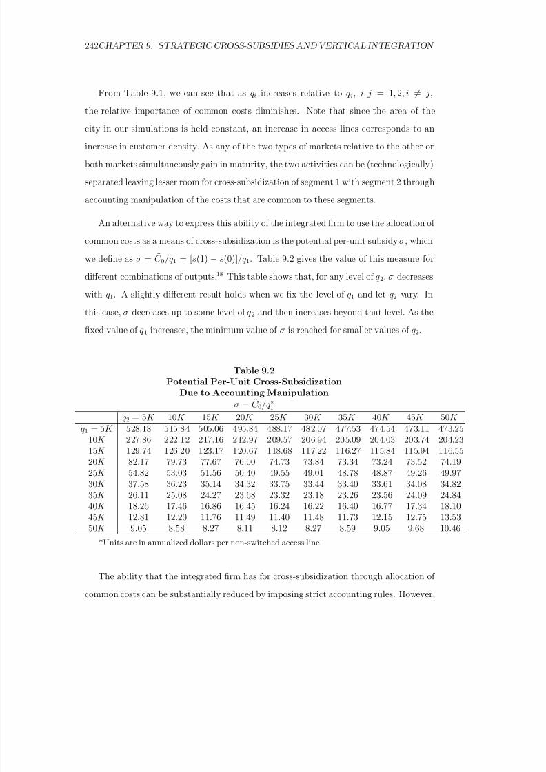
8/18/2019 Gasmi Cost Proxy Models
http://slidepdf.com/reader/full/gasmi-cost-proxy-models 242/318
242CHAPTER 9. STRATEGIC CROSS-SUBSIDIES AND VERTICAL INTEGRATION
From Table 9.1, we can see that as q i increases relative to q j, i, j = 1, 2, i = j,
the relative importance of common costs diminishes. Note that since the area of thecity in our simulations is held constant, an increase in access lines corresponds to an
increase in customer density. As any of the two types of markets relative to the other or
both markets simultaneously gain in maturity, the two activities can be (technologically)
separated leaving lesser room for cross-subsidization of segment 1 with segment 2 through
accounting manipulation of the costs that are common to these segments.
An alternative way to express this ability of the integrated firm to use the allocation of common costs as a means of cross-subsidization is the potential per-unit subsidy σ, which
we define as σ = C 0/q 1 = [s(1) − s(0)]/q 1. Table 9.2 gives the value of this measure for
different combinations of outputs.18 This table shows that, for any level of q 2, σ decreases
with q 1. A slightly different result holds when we fix the level of q 1 and let q 2 vary. In
this case, σ decreases up to some level of q 2 and then increases beyond that level. As the
fixed value of q 1 increases, the minimum value of σ is reached for smaller values of q 2.
Table 9.2Potential Per-Unit Cross-Subsidization
Due to Accounting Manipulation
σ = C 0/q ∗1q 2 = 5K 10K 15K 20K 25K 30K 35K 40K 45K 50K
q 1 = 5K 528.18 515.84 505.06 495.84 488.17 482.07 477.53 474.54 473.11 473.2510K 227.86 222.12 217.16 212.97 209.57 206.94 205.09 204.03 203.74 204.23
15K 129.74 126.20 123.17 120.67 118.68 117.22 116.27 115.84 115.94 116.5520K 82.17 79.73 77.67 76.00 74.73 73.84 73.34 73.24 73.52 74.1925K 54.82 53.03 51.56 50.40 49.55 49.01 48.78 48.87 49.26 49.9730K 37.58 36.23 35.14 34.32 33.75 33.44 33.40 33.61 34.08 34.8235K 26.11 25.08 24.27 23.68 23.32 23.18 23.26 23.56 24.09 24.8440K 18.26 17.46 16.86 16.45 16.24 16.22 16.40 16.77 17.34 18.1045K 12.81 12.20 11.76 11.49 11.40 11.48 11.73 12.15 12.75 13.5350K 9.05 8.58 8.27 8.11 8.12 8.27 8.59 9.05 9.68 10.46
*Units are in annualized dollars per non-switched access line.
The ability that the integrated firm has for cross-subsidization through allocation of
common costs can be substantially reduced by imposing strict accounting rules. However,
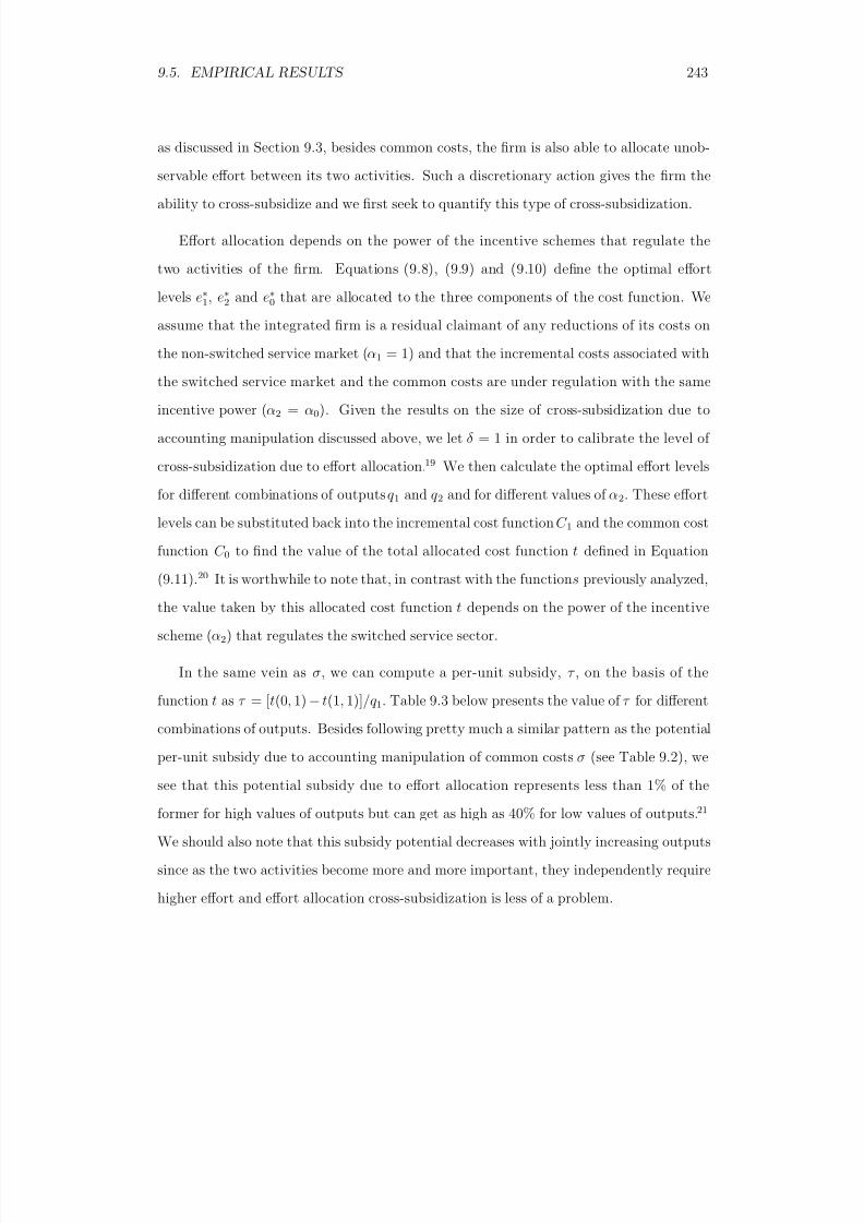
8/18/2019 Gasmi Cost Proxy Models
http://slidepdf.com/reader/full/gasmi-cost-proxy-models 243/318
9.5. EMPIRICAL RESULTS 243
as discussed in Section 9.3, besides common costs, the firm is also able to allocate unob-
servable effort between its two activities. Such a discretionary action gives the firm theability to cross-subsidize and we first seek to quantify this type of cross-subsidization.
Effort allocation depends on the power of the incentive schemes that regulate the
two activities of the firm. Equations (9.8), (9.9) and (9.10) define the optimal effort
levels e∗1, e∗2 and e∗0 that are allocated to the three components of the cost function. We
assume that the integrated firm is a residual claimant of any reductions of its costs on
the non-switched service market (α1 = 1) and that the incremental costs associated withthe switched service market and the common costs are under regulation with the same
incentive power (α2 = α0). Given the results on the size of cross-subsidization due to
accounting manipulation discussed above, we let δ = 1 in order to calibrate the level of
cross-subsidization due to effort allocation.19 We then calculate the optimal effort levels
for different combinations of outputs q 1 and q 2 and for different values of α2. These effort
levels can be substituted back into the incremental cost function C 1 and the common cost
function C 0 to find the value of the total allocated cost function t defined in Equation
(9.11).20 It is worthwhile to note that, in contrast with the function s previously analyzed,
the value taken by this allocated cost function t depends on the power of the incentive
scheme (α2) that regulates the switched service sector.
In the same vein as σ, we can compute a per-unit subsidy, τ , on the basis of the
function t as τ = [t(0, 1) − t(1, 1)]/q 1. Table 9.3 below presents the value of τ for different
combinations of outputs. Besides following pretty much a similar pattern as the potential
per-unit subsidy due to accounting manipulation of common costs σ (see Table 9.2), we
see that this potential subsidy due to effort allocation represents less than 1% of the
former for high values of outputs but can get as high as 40% for low values of outputs. 21
We should also note that this subsidy potential decreases with jointly increasing outputs
since as the two activities become more and more important, they independently require
higher effort and effort allocation cross-subsidization is less of a problem.
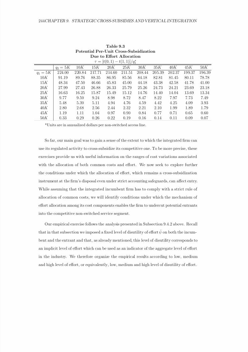
8/18/2019 Gasmi Cost Proxy Models
http://slidepdf.com/reader/full/gasmi-cost-proxy-models 244/318
244CHAPTER 9. STRATEGIC CROSS-SUBSIDIES AND VERTICAL INTEGRATION
Table 9.3
Potential Per-Unit Cross-SubsidizationDue to Effort Allocation
τ = [t(0, 1) − t(1, 1)]/q ∗1q 2 = 5K 10K 15K 20K 25K 30K 35K 40K 45K 50K
q 1 = 5K 224.00 220.84 217.71 214.60 211.51 208.44 205.39 202.37 199.37 196.3910K 91.19 89.76 88.35 86.95 85.56 84.18 82.81 81.45 80.11 78.7815K 48.34 47.50 46.66 45.83 45.00 44.18 43.38 42.58 41.78 41.0020K 27.99 27.43 26.88 26.33 25.79 25.26 24.73 24.21 23.69 23.1825K 16.63 16.25 15.87 15.49 15.12 14.76 14.40 14.04 13.69 13.3430K 9.77 9.50 9.24 8.98 8.72 8.47 8.22 7.97 7.73 7.49
35K 5.48 5.30 5.11 4.94 4.76 4.59 4.42 4.25 4.09 3.9340K 2.80 2.68 2.56 2.44 2.32 2.21 2.10 1.99 1.89 1.7945K 1.19 1.11 1.04 0.97 0.90 0.84 0.77 0.71 0.65 0.6050K 0.33 0.29 0.26 0.22 0.19 0.16 0.14 0.11 0.09 0.07
*Units are in annualized dollars per non-switched access line.
So far, our main goal was to gain a sense of the extent to which the integrated firm can
use its regulated activity to cross-subsidize its competitive one. To be more precise, these
exercises provide us with useful information on the ranges of cost variations associated
with the allocation of both common costs and effort. We now seek to explore further
the conditions under which the allocation of effort, which remains a cross-subsidization
instrument at the firm’s disposal even under strict accounting safeguards, can affect entry.
While assuming that the integrated incumbent firm has to comply with a strict rule of
allocation of common costs, we will identify conditions under which the mechanism of
effort allocation among its cost components enables the firm to undercut potential entrantsinto the competitive non-switched service segment.
Our empirical exercise follows the analysis presented in Subsection 9.4.2 above. Recall
that in that subsection we imposed a fixed level of disutility of effort ψ on both the incum-
bent and the entrant and that, as already mentioned, this level of disutility corresponds to
an implicit level of effort which can be used as an indicator of the aggregate level of effort
in the industry. We therefore organize the empirical results according to low, medium
and high level of effort, or equivalently, low, medium and high level of disutility of effort.
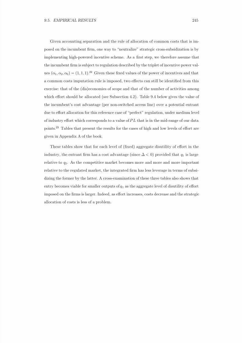
8/18/2019 Gasmi Cost Proxy Models
http://slidepdf.com/reader/full/gasmi-cost-proxy-models 245/318
9.5. EMPIRICAL RESULTS 245
Given accounting separation and the rule of allocation of common costs that is im-
posed on the incumbent firm, one way to “neutralize” strategic cross-subsidization is byimplementing high-powered incentive scheme. As a first step, we therefore assume that
the incumbent firm is subject to regulation described by the triplet of incentive power val-
ues (α1, α2, α0) = (1, 1, 1).22 Given these fixed values of the power of incentives and that
a common costs imputation rule is imposed, two effects can still be identified from this
exercise: that of the (dis)economies of scope and that of the number of activities among
which effort should be allocated (see Subsection 4.2). Table 9.4 below gives the value of
the incumbent’s cost advantage (per non-switched access line) over a potential entrant
due to effort allocation for this reference case of “perfect” regulation, under medium level
of industry effort which corresponds to a value of P L that is in the mid-range of our data
points.23 Tables that present the results for the cases of high and low levels of effort are
given in Appendix A of the book.
These tables show that for each level of (fixed) aggregate disutility of effort in the
industry, the entrant firm has a cost advantage (since ∆ < 0) provided that q 1 is large
relative to q 2. As the competitive market becomes more and more and more important
relative to the regulated market, the integrated firm has less leverage in terms of subsi-
dizing the former by the latter. A cross-examination of these three tables also shows that
entry becomes viable for smaller outputs of q 1 as the aggregate level of disutility of effort
imposed on the firms is larger. Indeed, as effort increases, costs decrease and the strategic
allocation of costs is less of a problem.
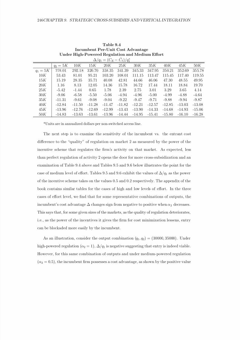
8/18/2019 Gasmi Cost Proxy Models
http://slidepdf.com/reader/full/gasmi-cost-proxy-models 246/318
246CHAPTER 9. STRATEGIC CROSS-SUBSIDIES AND VERTICAL INTEGRATION
Table 9.4
Incumbent Per-Unit Cost AdvantageUnder High-Powered Regulation and Medium Effort
∆/q 1 = (C E − C I )/q ∗1q 2 = 5K 10K 15K 20K 25K 30K 35K 40K 45K 50K
q 1 = 5K 224.01 292.18 320.70 334.35 341.39 345.33 347.95 350.21 352.69 355.7810K 53.43 81.01 95.21 103.20 108.01 111.15 113.47 115.45 117.40 119.5515K 15.19 28.35 35.71 40.08 42.81 44.66 46.06 47.30 48.55 49.9520K 1.16 8.13 12.05 14.36 15.78 16.72 17.44 18.11 18.84 19.7025K -5.42 -1.44 0.65 1.78 2.39 2.75 3.01 3.29 3.65 4.1430K -9.06 -6.58 -5.50 -5.06 -4.94 -4.96 -5.00 -4.99 -4.88 -4.64
35K -11.31 -9.61 -9.08 -9.04 -9.22 -9.47 -9.71 -9.88 -9.94 -9.8740K -12.84 -11.50 -11.28 -11.47 -11.82 -12.21 -12.57 -12.85 -13.03 -13.0845K -13.96 -12.76 -12.69 -12.99 -13.43 -13.90 -14.33 -14.68 -14.93 -15.0650K -14.83 -13.63 -13.61 -13.96 -14.44 -14.95 -15.41 -15.80 -16.10 -16.28
*Units are in annualized dollars per non-switched access line.
The next step is to examine the sensitivity of the incumbent vs. the entrant cost
difference to the “quality” of regulation on market 2 as measured by the power of the
incentive scheme that regulates the firm’s activity on that market. As expected, less
than perfect regulation of activity 2 opens the door for more cross-subsidization and an
examination of Table 9.4 above and Tables 9.5 and 9.6 below illustrates the point for the
case of medium level of effort. Tables 9.5 and 9.6 exhibit the values of ∆ /q 1 as the power
of the incentive scheme takes on the values 0.5 and 0.2 respectively. The appendix of the
book contains similar tables for the cases of high and low levels of effort. In the three
cases of effort level, we find that for some representative combinations of outputs, the
incumbent’s cost advantage ∆ changes sign from negative to positive when α2 decreases.
This says that, for some given sizes of the markets, as the quality of regulation deteriorates,
i.e., as the power of the incentives it gives the firm for cost minimization lessens, entry
can be blockaded more easily by the incumbent.
As an illustration, consider the output combination (q 1, q 2) = (30000, 35000). Under
high-powered regulation (α2 = 1), ∆/q 1 is negative suggesting that entry is indeed viable.
However, for this same combination of outputs and under medium-powered regulation
(α2 = 0.5), the incumbent firm possesses a cost advantage, as shown by the positive value
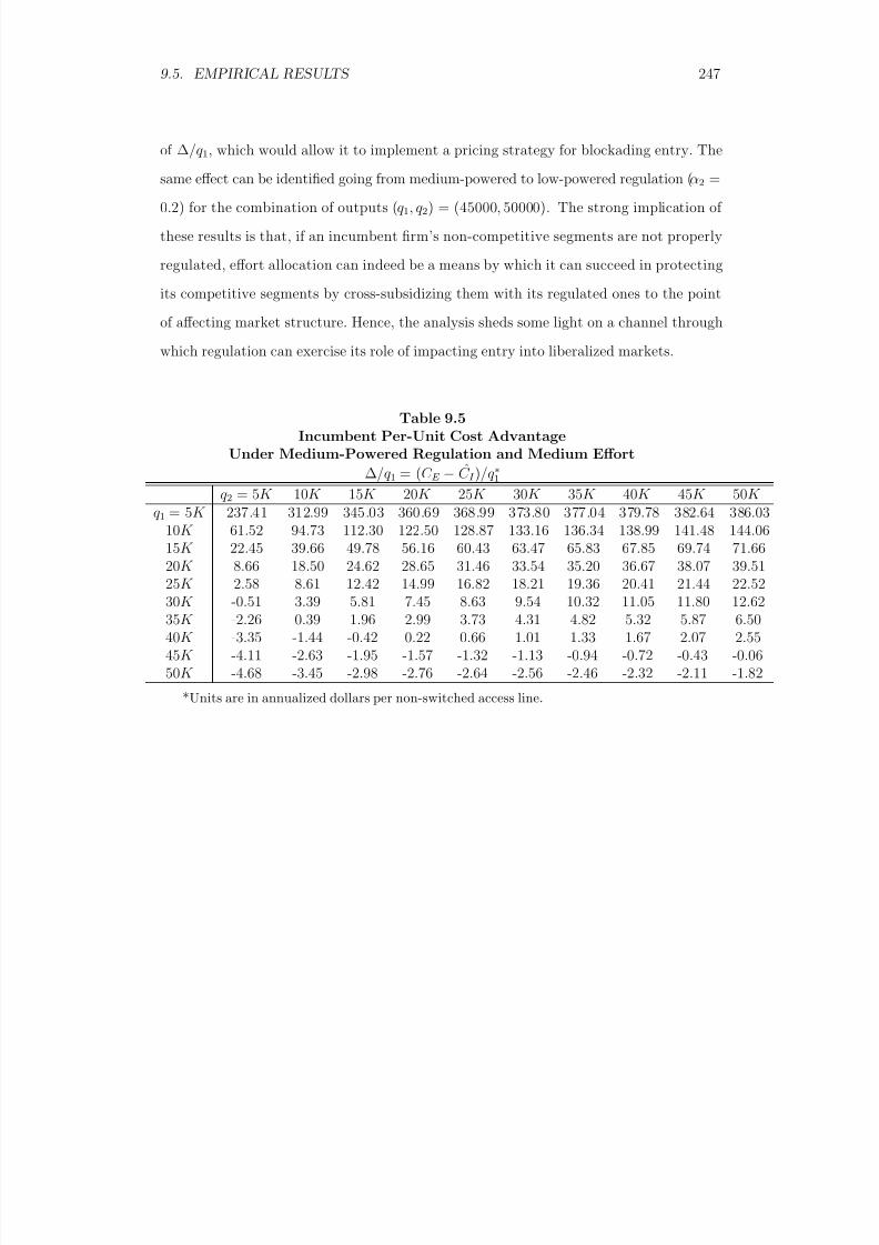
8/18/2019 Gasmi Cost Proxy Models
http://slidepdf.com/reader/full/gasmi-cost-proxy-models 247/318
9.5. EMPIRICAL RESULTS 247
of ∆/q 1, which would allow it to implement a pricing strategy for blockading entry. The
same effect can be identified going from medium-powered to low-powered regulation (α2 =0.2) for the combination of outputs (q 1, q 2) = (45000, 50000). The strong implication of
these results is that, if an incumbent firm’s non-competitive segments are not properly
regulated, effort allocation can indeed be a means by which it can succeed in protecting
its competitive segments by cross-subsidizing them with its regulated ones to the point
of affecting market structure. Hence, the analysis sheds some light on a channel through
which regulation can exercise its role of impacting entry into liberalized markets.
Table 9.5Incumbent Per-Unit Cost Advantage
Under Medium-Powered Regulation and Medium Effort
∆/q 1 = (C E − C I )/q ∗1q 2 = 5K 10K 15K 20K 25K 30K 35K 40K 45K 50K
q 1 = 5K 237.41 312.99 345.03 360.69 368.99 373.80 377.04 379.78 382.64 386.0310K 61.52 94.73 112.30 122.50 128.87 133.16 136.34 138.99 141.48 144.06
15K 22.45 39.66 49.78 56.16 60.43 63.47 65.83 67.85 69.74 71.6620K 8.66 18.50 24.62 28.65 31.46 33.54 35.20 36.67 38.07 39.5125K 2.58 8.61 12.42 14.99 16.82 18.21 19.36 20.41 21.44 22.5230K -0.51 3.39 5.81 7.45 8.63 9.54 10.32 11.05 11.80 12.6235K -2.26 0.39 1.96 2.99 3.73 4.31 4.82 5.32 5.87 6.5040K -3.35 -1.44 -0.42 0.22 0.66 1.01 1.33 1.67 2.07 2.5545K -4.11 -2.63 -1.95 -1.57 -1.32 -1.13 -0.94 -0.72 -0.43 -0.0650K -4.68 -3.45 -2.98 -2.76 -2.64 -2.56 -2.46 -2.32 -2.11 -1.82
*Units are in annualized dollars per non-switched access line.
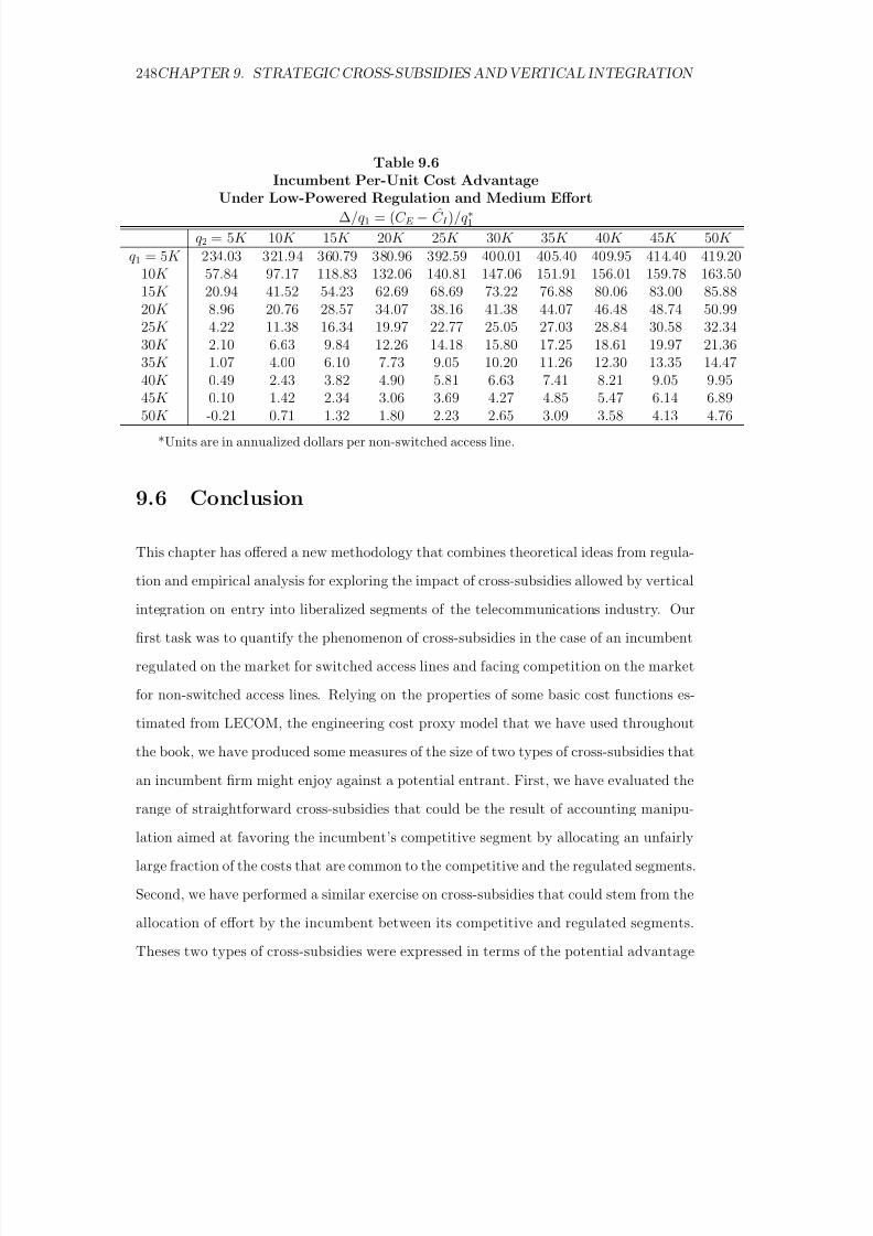
8/18/2019 Gasmi Cost Proxy Models
http://slidepdf.com/reader/full/gasmi-cost-proxy-models 248/318
248CHAPTER 9. STRATEGIC CROSS-SUBSIDIES AND VERTICAL INTEGRATION
Table 9.6
Incumbent Per-Unit Cost AdvantageUnder Low-Powered Regulation and Medium Effort
∆/q 1 = (C E − C I )/q ∗1q 2 = 5K 10K 15K 20K 25K 30K 35K 40K 45K 50K
q 1 = 5K 234.03 321.94 360.79 380.96 392.59 400.01 405.40 409.95 414.40 419.2010K 57.84 97.17 118.83 132.06 140.81 147.06 151.91 156.01 159.78 163.5015K 20.94 41.52 54.23 62.69 68.69 73.22 76.88 80.06 83.00 85.8820K 8.96 20.76 28.57 34.07 38.16 41.38 44.07 46.48 48.74 50.9925K 4.22 11.38 16.34 19.97 22.77 25.05 27.03 28.84 30.58 32.3430K 2.10 6.63 9.84 12.26 14.18 15.80 17.25 18.61 19.97 21.36
35K 1.07 4.00 6.10 7.73 9.05 10.20 11.26 12.30 13.35 14.4740K 0.49 2.43 3.82 4.90 5.81 6.63 7.41 8.21 9.05 9.9545K 0.10 1.42 2.34 3.06 3.69 4.27 4.85 5.47 6.14 6.8950K -0.21 0.71 1.32 1.80 2.23 2.65 3.09 3.58 4.13 4.76
*Units are in annualized dollars per non-switched access line.
9.6 Conclusion
This chapter has offered a new methodology that combines theoretical ideas from regula-
tion and empirical analysis for exploring the impact of cross-subsidies allowed by vertical
integration on entry into liberalized segments of the telecommunications industry. Our
first task was to quantify the phenomenon of cross-subsidies in the case of an incumbent
regulated on the market for switched access lines and facing competition on the market
for non-switched access lines. Relying on the properties of some basic cost functions es-
timated from LECOM, the engineering cost proxy model that we have used throughoutthe book, we have produced some measures of the size of two types of cross-subsidies that
an incumbent firm might enjoy against a potential entrant. First, we have evaluated the
range of straightforward cross-subsidies that could be the result of accounting manipu-
lation aimed at favoring the incumbent’s competitive segment by allocating an unfairly
large fraction of the costs that are common to the competitive and the regulated segments.
Second, we have performed a similar exercise on cross-subsidies that could stem from the
allocation of effort by the incumbent between its competitive and regulated segments.
Theses two types of cross-subsidies were expressed in terms of the potential advantage
8/18/2019 Gasmi Cost Proxy Models
http://slidepdf.com/reader/full/gasmi-cost-proxy-models 249/318
9.6. CONCLUSION 249
per non-switched access line that the incumbent would have over a potential entrant. This
measure gives us an idea of the extent to which the incumbent can (unfairly) undercutits competitors.
While the adverse effect on entry of the first type of cross-subsidy can to a large extent
be alleviated by imposing strong accounting safeguards, because effort is inherently unob-
servable, the second type of cross-subsidy is considerably more difficult for the regulator
to deal with. Our primary objective in this chapter has been to explore the impact of
this type of cross-subsidy on the process of entry into liberalized segments. The fact thatwe are able with LECOM to proxy effort allows us to closely examine the mechanism by
which the incumbent allocates effort among its (regulated) switched service segment and
its (competitive) non-switched segments. New regulatory theory is called upon to analyze
this mechanism of effort allocation. Specifically, we emphasize the role of the power of
the incentive scheme that regulates the incumbent, and by endogenizing costs due to the
form of regulation, we identify situations where the incumbent can achieve lower costs
than a potential competitor. Our analysis illustrates that regulation, which is designed
to foster competition, may, in fact, hinder competition if it does not give the incumbent
firm appropriate incentives to efficiently allocate managerial effort among the divisions of
the firm.

8/18/2019 Gasmi Cost Proxy Models
http://slidepdf.com/reader/full/gasmi-cost-proxy-models 250/318
250 NOTES
Notes
1Under structural safeguards, local telephone companies are required to maintain a
strict separation between the regulated and unregulated sectors of the company (see
FCC, 1971, 1980 and 1999). The separation requirements include separate corporate
structures, operating facilities and physical locations. Information flows among divisions
and joint marketing arrangements are also restricted. Accounting safeguards allow the
firm to deploy labor and other inputs freely among divisions, but impose cost allocation
rules to separate the costs of the firm into regulated and unregulated sectors.
2The expression given in (9.2) also allows for disutility to depend upon output levels.
The implications of this assumption in the context of optimal regulation under incomplete
information have been discussed in Chapters 4 and 6.
3The higher the fraction of costs born by a firm, i.e, the larger the costs for which it
is accountable, the higher its incentives to minimize them. This fraction is referred to in
the literature as the “power” of the underlying incentive scheme (see Chapter 4 for more
details).
4These assumptions would be appropriate in situations where entrants make use of
the incumbent’s network through the purchase of unbundled network elements. In the
United States, network elements are priced according to a TELRIC (Total Element Long
Run Incremental Cost) methodology, which is interpreted as incremental cost plus a “rea-
sonable” contribution to common costs. Later in this section we consider an alternative
model of facilities based entry.
5For given levels of outputs, this disutility is the result of an implicit level of effort e,
say, which can be used as an indicator of the general level of effort in the industry. (For
example, effort can be considered to be “high”, “medium” or “low”.)
6Note that a positive ∆ would suggest that entry can potentially be blockaded.
7Chapter 5 contains an analysis of the cost of access lines as a function of overall

8/18/2019 Gasmi Cost Proxy Models
http://slidepdf.com/reader/full/gasmi-cost-proxy-models 251/318
NOTES 251
customer density, where the relative densities of the urban and rural sectors was held con-
stant. In Chapter 8 we look at cost functions for the urban and rural sectors individually.
8With a total subscriber population of 100, 000 spread over a city with a total area
of about 57.5 square miles, the customer densities in our simulation are 1006 subscribers
per square mile in the residential district, 2278 per square mile in the mixed district and
7260 per square mile in the business district. In the simulations, when total subscriber
population varies, the densities of the districts relative to each others are maintained
constant.
9The actual total numbers of access lines were 6000, 12000, 20000, 40000, 70000 and
100000.
10More specifically, P K, P L = 0.6, 0.8, 1.0, 1.2, 1.4.
11See below for more on the relationship between the theoretical cost functions and
their empirical counterparts.
12The simulations produced data sets of 900 points. Because some of our cost functions
require having a zero as an argument, we fit our LECOM cost data to a functional form
which is a second-degree polynomial of the appropriate variables rather than their natural
logarithms as done in the previous chapters. The expression of the various cost functions
used in this chapter is given in Appendix A of the book.
13For clarity of exposition, in this chapter we adopt the convention of designating by C
the (LECOM-estimated) empirical counterpart of a generic theoretical cost function C .
14Recall that in our analysis, there is a one-to-one correspondence between the set of
values of P L and that of values of e. This correspondence is defined by the relation
e = 1.5 − P L.
15
The combinations of output levels for which these calculations were made can be seenfrom the next subsection.

8/18/2019 Gasmi Cost Proxy Models
http://slidepdf.com/reader/full/gasmi-cost-proxy-models 252/318
252 NOTES
16This is true provided that the firm is regulated with a cost-plus type scheme.
17Note that in the notation of Section 9.2, this measure is equal to [(s(1)−s(0))/C ]×100.
18To have an idea of the relative importance of these per-access line potential subsidies,
a table provides the value of average cost for different values of outputs in Appendix A.
19By allocating entirely the common costs to segment 1 (δ = 1), the aim is to obtain
the most significant effort allocation cross-subsidization effect.
20Recall that the function t(α2, δ ) measures the allocated cost of activity 1 given the
common costs allocation parameter δ and the fraction α2 of the incremental cost of activity
2 born by the incumbent.
21We should note though that the non-monotonicity of σ found when q 1 is fixed and q 2
varies does not occur in the case of τ .
22Note that regulation here is implicit for the case of activity 1 which is competitive.
23By perfect regulation we mean here regulation with a high-powered scheme.
8/18/2019 Gasmi Cost Proxy Models
http://slidepdf.com/reader/full/gasmi-cost-proxy-models 253/318
Chapter 10
Conclusion
We initiated this line of research in the Fall of 1994. At that time the theory of incentive
regulation was already well developed, but it was becoming increasingly apparent that the
prospects for empirical tests of the theory were limited. One source of difficulty, at least
for empirical tests of the theory of regulation in the telecommunications industry, is the
relatively poor quality of data for firms in that industry.1 Historical data are recorded at
most on a quarterly basis, and for a limited number of firms, since the industry has been
characterized by regulated or public monopoly for most of its history. Thus, the oppor-
tunity to construct meaningful time series or panels sets of data for firms facing different
regulatory constraints has been limited. Furthermore, the available data are generally
presented in highly aggregate form, and in categories based on accounting purposes that
are not necessarily appropriate for an analysis of incentive effects. 2
A more significant barrier to empirical analysis, however, is the nature of the testable
implications that the theory suggests. As our survey in Chapter 4 illustrates, it is possible
to characterize fully the social welfare consequences of various forms of regulation, and
other chapters pursue a similar approach to a wide variety of policy issues in the industry.
A common theme of these chapters is that the testable implications of the theory, in large
part, depend on very detailed properties of the cost function of a representative firm in the
industry. For example, in the characterization of optimal regulation of a natural monopolysupplier, the optimal mechanism is shown to depend on the detailed relationship of the
253

8/18/2019 Gasmi Cost Proxy Models
http://slidepdf.com/reader/full/gasmi-cost-proxy-models 254/318
254 CHAPTER 10. CONCLUSION
derivatives of the cost function with respect to technology and effort. Using historical
data, it would be difficult to adequately characterize these relationships.
Very early in this project we therefore began to consider an alternative approach to
cost estimation using engineering process, or cost proxy, models. We were aware of a
long tradition of economic analysis using engineering models, but the real impetus to our
research program was the discovery of a recently developed public domain proxy model
of local exchange telephony.3 Given a proxy model as a tool, we had a clear idea of our
research objectives, but we still did not have a well conceived plan for achieving thoseobjectives. Our endeavor was very much an exercise in learning by doing. To some extent,
as we proceeded by trial and error in using the model to generate data for our empirical
analysis, our research objectives were correspondingly modified. In the remainder of this
chapter we describe briefly the most important results of our research program to date,
the methodological lessons that we have learned, and some directions for future research.
10.1 What Have We Learned?
10.1.1 Implications for incentive regulation and telecommuni-cations policy
Our primary objective was to fully characterize the cost function of a representative
local exchange telecommunications firm, and to apply this representation to a variety of
economic models representing current issues in telecommunications policy. The major
innovation in the cost analysis was to allow for incomplete information of the regulator,
a cornerstone of the new economics of regulation. In this we believe that our efforts have
been successful, although our representation of the technology is admittedly crude and
capable of substantial refinement. We will consider in later sections of this chapter some
of the promising areas for future refinements of our analysis, but in this section let us
briefly summarize some of the main conclusions of our efforts to date.
We began in Chapter 5 with a reexamination of the proper characterization of natural
8/18/2019 Gasmi Cost Proxy Models
http://slidepdf.com/reader/full/gasmi-cost-proxy-models 255/318
10.1. WHAT HAVE WE LEARNED? 255
monopoly in a traditionally regulated industry such as local telecommunications. Con-
ceptually, our analysis led us to suggest that a proper definition of natural monopolyshould take account not only of the traditional technological characteristics of the indus-
try, i.e., the properties of the cost function alone, but in addition a variety of social welfare
measures.
We considered two entry scenarios. Under targeted entry an entrant succeeds in ul-
timately attracting all of the customers in a portion of the incumbent’s service territory.
Under uniform entry both the incumbent and entrant share the entire market territory,and customer densities for each firm depend on their respective market shares. We also
made various strong assumptions on the basis of a few simple economic models of the
regulatory regime and firm behavior under both monopoly and free entry duopoly. In our
“access as usage” model, we found that the performance of a deregulated market clearly
depends on the assumptions made about the way firms compete. Under either regulated
(i.e. yardstick) competition or highly competitive unregulated competition, we found
that duopoly outperforms traditional cost plus regulated monopoly under both uniform
and targeted entry scenarios. Under the more favorable targeted entry scenario, yard-
stick competition outperforms simple price cap regulation, while competitive unregulated
duopoly achieves slightly lower aggregate social welfare than incentive regulation.
In Chapter 6 we considered in detail some of the properties of optimal incentive regu-
lation. As noted above, this is a task that requires a detailed representation of the firm’s
cost function with respect to its technology and managerial effort input variables. Based
on this representation, and some additional (perhaps heroic) assumptions about consumer
demand, the nature of the firm’s disutility of effort function and the regulator’s beliefs, we
were able to explicitly solve for the optimal regulatory contract. This contract specifies
the output for the firm to produce and the transfer that the regulator will make to the
firm at each level of output. We were also able to demonstrate that optimal regulation
could be approximately determined by prices set according to the Ramsey rule plus a
monetary transfer to the firm.4 In addition, the optimal transfer can be implemented by

8/18/2019 Gasmi Cost Proxy Models
http://slidepdf.com/reader/full/gasmi-cost-proxy-models 256/318
256 CHAPTER 10. CONCLUSION
a menu of linear contracts presented to the regulated firm.
In Chapter 7 we extended our analysis of regulated monopoly by considering a variety
of regulatory mechanisms which differ in the quality of information available to the reg-
ulator and in the feasibility of making transfers to the regulated firm. Full information
(a benchmark but not a realistic prospect for any regulator) requires the observability
of both cost and effort. Cost observability (ex post) requires minimal accounting pro-
cedures, while other mechanisms such as price caps do not rely on any observation of
current cost. Transfers can be bi-directional, in which case they can be used to induce thefirm to choose an efficient (at the margin) level of effort given the transfer. Alternatively,
a uni-directional transfer from the firm to the regulator (and consumers) can be used
to improve the distributional consequences of the regulatory mechanism. Our analysis
confirms the widely held belief that incentive regulation generally, including the widely
observed use of simple price caps, can significantly increase aggregate social welfare rela-
tive to traditional cost plus regulation. However, pure price cap regulation and pure cost
plus regulation have vastly different distributional consequences, with price caps favoring
the profits of the regulated firm and cost plus favoring the welfare of consumers. Opti-
mal incentive regulation, in our simulations, offers consumers a welfare level close to that
achieved under cost plus, while allowing the firm to achieve rents that are also close to
the rents they achieve under price caps. Somewhat surprisingly, a price cap mechanism
with profit sharing achieves a very similar result.
In Chapter 8 we again considered the role of competition policy and deregulation in
the context of a public mandate to finance a universal service subsidy to telecommunica-
tions customers in high cost areas. We modeled the cost structure of a service territory
consisting of a low cost urban area and a higher cost rural area. We assumed in an “ur-
ban targeted” scenario that if entry is unconstrained, a rational entrant would choose to
serve only the lower cost urban customers. In this case, Bertrand-like price competition
is assumed to determine the price in the urban market, while the regulated incumbent
is faced with a universal service obligation to serve rural customers at the same price.

8/18/2019 Gasmi Cost Proxy Models
http://slidepdf.com/reader/full/gasmi-cost-proxy-models 257/318
10.1. WHAT HAVE WE LEARNED? 257
The implied budget deficit for the incumbent is assumed to be financed through a public
subsidy. As an alternative, in a “territory constrained” scenario, the regulator could im-pose a universal service obligation on both the entrant and the incumbent firm. In this
case, the universal service objective can be achieved under competition without the use
of a public subsidy, but the price to urban (and rural) customers is higher than under the
urban targeted scenario.
Our analysis reveals that the cross subsidies implicit in the territory constrained sce-
nario may be an efficient method of financing the universal service objective if the costof public funds (given by λ) is sufficiently high. In fact, under complete information,
the territory constrained scenario dominates the urban targeted scenario for virtually all
reasonable values of λ. A similar result holds under price cap regulation (for the territory
constrained scenario) though for higher critical values of λ.
Finally in Chapter 9 we considered an issue of some importance in newly deregulated
telecommunications markets. We considered the case in which some markets are fully open
(and attractive) to competitive entrants, while other markets are served exclusively by the
incumbent monopolist. Nevertheless, the incumbent monopoly is assumed to participate
in the unregulated markets, and this participation raises the issue of cross subsidization
between regulated and unregulated activities of the incumbent. Using LECOM we sim-
ulated the cost structure of a firm which serves markets for both switched access lines,
which we assumed to be fully regulated, and non-switched access lines, which we assumed
to be competitive. We then decomposed the resulting cost function into a common cost
term and incremental costs associated with the regulated and unregulated activities, and
based on this decomposition derived a cost function for firms serving only the unregulated
market.
We were able to characterize both the magnitude of cross subsidies due to accounting
manipulation and cross subsidies that could result from the allocation of effort by the
incumbent firm between regulated and unregulated activities. We found that strategic
cross subsidies (due to effort allocation) are always lower in magnitude than account-

8/18/2019 Gasmi Cost Proxy Models
http://slidepdf.com/reader/full/gasmi-cost-proxy-models 258/318
258 CHAPTER 10. CONCLUSION
ing cross subsidies, but for lower values of output reflecting small scale entry, they are
nevertheless significant. Since accounting cross subsidy can, in principle, be easily ob-served and controlled by accounting safeguards, while effort misallocation is difficult or
impossible to observe, the latter finding is significant. We further examined the potential
role of strategic cross subsidies by asking whether, under strict accounting safeguards,
a regulated incumbent can use its ability to allocate effort strategically to blockade the
entry of an otherwise efficient entrant. This analysis revealed that the possibility of entry
deterrence depends critically on the power of the regulatory incentive scheme.
10.1.2 Lessons for the use of proxy models in empirical research
In addition to the policy implications that we were able to draw on the basis of our
characterization of the cost function for local telecommunications, there were some useful
lessons learned on the use of proxy models in an empirical research program. These can
be grouped broadly into data issues, including the choice of proxies for technology and
managerial effort, computational issues, and the extension of the proxy model approach
to new markets and new technologies.
One of the first issues to be decided was the definition of an appropriate set of inputs
and outputs for a telecommunications cost function. From our theoretical presentation,
recall that we have consistently assumed that a cost function could be represented in a
form C (β, e, q ) where β represents a technology parameter (known to the firm but notthe regulator), e represents cost reducing effort by the firm that is not observable by
the regulator and q represents output. Tables A.7 and A.8 in the Appendix illustrate
representative LECOM input and output files from which prospective inputs and outputs
could be chosen. As indicated, the output file represents the total annual cost of a serving
area, which is broken down into the cost of distribution plant, feeder plant, switching
plant, interoffice plant, and the cost of the main distribution frame. As potential quantity
variables, LECOM specifies the number of switched access lines and the number of private
lines (both distributed among business, mixed and residential lines), traffic volume per
8/18/2019 Gasmi Cost Proxy Models
http://slidepdf.com/reader/full/gasmi-cost-proxy-models 259/318
10.1. WHAT HAVE WE LEARNED? 259
line measured in CCS (also distributed among business, mixed and residential lines) and
the ratio of local to toll usage. In each of the empirical chapters we have used one or moreof these variables to represent the cost function for a local exchange company.
A somewhat more difficult task was the choice of a pair of input parameters to represent
β and e. Initially we considered using a specific technological input variable, such as
“plcost” (the cost markup for private access lines due to additional line conditioning and
higher reliability standards traditionally required by business customers) or the utilization
rate (giving spare capacity when loop and switching plant is deployed). Experimentswith these input variables did not prove successful, however, largely because the range of
cost variation for plausible ranges of input variation was not significant when all other
inputs were held constant. As a proxy for managerial effort, e, we briefly considered the
theoretically attractive possibility of using the LECOM optimization parameters “ftol”
and “itmax” (which essentially instructed the computer algorithm how hard to search for
an optimal solution). However, these experiments also produced only minor cost variation,
and had the added drawback of introducing a significant noise factor for low levels of
computer “effort.” We therefore settled on the convenient, but perhaps unintuitive, choice
of the variables P K and P L to represent technology and effort. As explained elsewhere,
P K and P L both act as a multiplier for a large number of other LECOM input parameters
that have an impact on the capital and labor inputs to production respectively. We thus
assumed that technology is embodied in the capital stock of a representative firm and
that effort is a function of the labor input, which we interpret as the efficiency price of
labor, and we have maintained this assumption throughout our analysis.
Given the full set of quantity and price input variables, we next created a grid of values
and proceeded to generate a set of “pseudo-data” through a large number of simulations.
Since the number of potential data points was limited only by the speed and number of
computers used for these simulations, our first intention was to create a very large data set
in order to conduct an analytical analysis based on the resulting discrete data.5
We found,
however, that the interpretation of the discrete data was difficult for several reasons. For

8/18/2019 Gasmi Cost Proxy Models
http://slidepdf.com/reader/full/gasmi-cost-proxy-models 260/318
260 CHAPTER 10. CONCLUSION
example, the characterization of optimal incentive regulation depends on a solution of
first order conditions involving the ratio of partial derivatives of the cost function withrespect to β and e. Since LECOM generates only an estimate of minimum cost for any
given set of inputs, we found that in some cases the realized values of the cost function
were not monotonic functions of these input parameters. Even when the cost difference
at adjacent data points had the expected sign, the process of computing two sets of first
differences and taking their ratio proved to introduce a noise factor that made it difficult
to accurately characterize a unique solution.
Rather than simply discarding data points representing non-monotonic cost values or
working with a smoothed set of discrete data, we decided to take the simpler approach of
using the entire data set to estimate a smooth functional form cost function. Following a
long tradition of empirical analysis, we used a translog functional form and were able to
successfully generate a smooth numerical valued cost function. We did not impose any
of the standard restrictions on the functional form of the cost function, such as input
price homogeneity. It is worth noting, however, that in our case the data-generating
process relies on an explicit cost minimization algorithm which by construction satisfies
the required homogeneity conditions. Any violation of standard constraints on the cost
function parameters could only be an indication of a computational error in the network
optimization or the imprecision of the translog approximation to the true underlying cost
function. We did not find evidence of either effect.
The use of a translog involved certain compromises in subsequent analysis. For ex-
ample, a translog function is not well defined for values of inputs or outputs near the
origin. We defined the effort variable by (P L0 − P L) for values of P L < P L0, where
P L0 represents the efficiency price of labor associated with minimal effort. Therefore, our
empirical cost function was not well defined for small effort levels, and it was necessary to
take this into account where theory suggests that solutions at minimal effort are possible.
Similarly, in our analysis of cross subsidy in Chapter 9 it was necessary to obtain a cost
function representation of the fixed and variable costs, so that outputs at zero were nec-
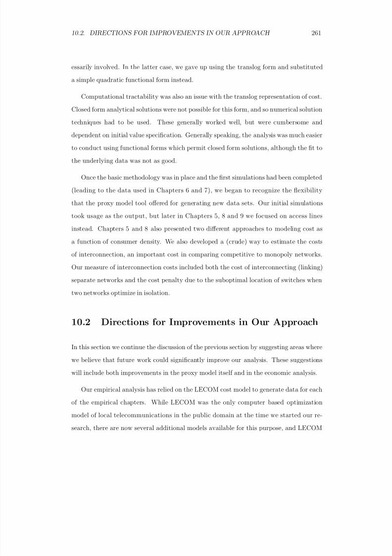
8/18/2019 Gasmi Cost Proxy Models
http://slidepdf.com/reader/full/gasmi-cost-proxy-models 261/318
10.2. DIRECTIONS FOR IMPROVEMENTS IN OUR APPROACH 261
essarily involved. In the latter case, we gave up using the translog form and substituted
a simple quadratic functional form instead.
Computational tractability was also an issue with the translog representation of cost.
Closed form analytical solutions were not possible for this form, and so numerical solution
techniques had to be used. These generally worked well, but were cumbersome and
dependent on initial value specification. Generally speaking, the analysis was much easier
to conduct using functional forms which permit closed form solutions, although the fit to
the underlying data was not as good.
Once the basic methodology was in place and the first simulations had been completed
(leading to the data used in Chapters 6 and 7), we began to recognize the flexibility
that the proxy model tool offered for generating new data sets. Our initial simulations
took usage as the output, but later in Chapters 5, 8 and 9 we focused on access lines
instead. Chapters 5 and 8 also presented two different approaches to modeling cost as
a function of consumer density. We also developed a (crude) way to estimate the costs
of interconnection, an important cost in comparing competitive to monopoly networks.
Our measure of interconnection costs included both the cost of interconnecting (linking)
separate networks and the cost penalty due to the suboptimal location of switches when
two networks optimize in isolation.
10.2 Directions for Improvements in Our Approach
In this section we continue the discussion of the previous section by suggesting areas where
we believe that future work could significantly improve our analysis. These suggestions
will include both improvements in the proxy model itself and in the economic analysis.
Our empirical analysis has relied on the LECOM cost model to generate data for each
of the empirical chapters. While LECOM was the only computer based optimization
model of local telecommunications in the public domain at the time we started our re-
search, there are now several additional models available for this purpose, and LECOM
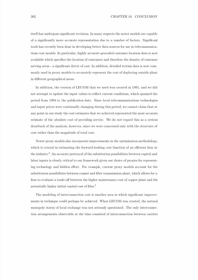
8/18/2019 Gasmi Cost Proxy Models
http://slidepdf.com/reader/full/gasmi-cost-proxy-models 262/318
262 CHAPTER 10. CONCLUSION
itself has undergone significant revisions. In many respects the newer models are capable
of a significantly more accurate representation due to a number of factors. Significantwork has recently been done in developing better data sources for use in telecommunica-
tions cost models. In particular, highly accurate geocoded customer location data is now
available which specifies the location of customers and therefore the density of customer
serving areas - a significant driver of cost. In addition, detailed terrain data is now com-
monly used in proxy models to accurately represent the cost of deploying outside plant
in different geographical areas.
In addition, the version of LECOM that we used was created in 1991, and we did
not attempt to update the input values to reflect current conditions, which spanned the
period from 1994 to the publication date. Since local telecommunications technologies
and input prices were continually changing during this period, we cannot claim that at
any point in our study the cost estimates that we achieved represented the most accurate
estimate of the absolute cost of providing service. We do not regard this as a serious
drawback of the analysis, however, since we were concerned only with the structure of
cost rather than the magnitude of total cost.
Newer proxy models also incorporate improvements in the optimization methodology,
which is crucial in estimating the forward-looking cost function of an efficient firm in
the industry.6 An accurate portrayal of the substitution possibilities between capital and
labor inputs is clearly critical to our framework given our choice of proxies for represent-
ing technology and hidden effort. For example, current proxy models account for the
substitution possibilities between copper and fiber transmission plant, which allows for a
firm to evaluate a trade-off between the higher maintenance cost of copper plant and the
potentially higher initial capital cost of fiber.7
The modeling of interconnection cost is another area in which significant improve-
ments in technique could perhaps be achieved. When LECOM was created, the natural
monopoly status of local exchange was not seriously questioned. The only interconnec-
tion arrangements observable at the time consisted of interconnection between carriers
8/18/2019 Gasmi Cost Proxy Models
http://slidepdf.com/reader/full/gasmi-cost-proxy-models 263/318
10.2. DIRECTIONS FOR IMPROVEMENTS IN OUR APPROACH 263
serving customers in separate jurisdictions, and there were no serious attempts to model
the costs of interconnecting such carriers. In theory, we believe that our approach to in-terconnection is sound, since it computes the difference between the costs of two carriers
optimizing in isolation and the cost of a single firm serving the entire market. However,
in practice, it is relatively cumbersome to follow this approach, and as a result we used
it to compute only a single interconnection multiplier for equal sized competitors, which
we then applied to all outputs of the interconnecting carriers. This approach is likely to
overstate the cost of interconnection when the two carriers differ significantly in size. In
addition, interconnection costs depend in large part on the cost structure of switching
machines, and it is not clear that LECOM or any of the more recent proxy models are
able to accurately represent this cost.
Perhaps the largest single area for improvement in our analysis is the development of
better proxies for technology and hidden effort. While we are generally comfortable with
the choice of P K as a proxy for technology, it would be desirable to have available an
alternative more direct measure of technology. The use of P L as a proxy for effort is even
more troublesome. It is possible that some of the newer proxy models, such as the HCPM
model described in an appendix, could be used to provide a better proxy for the labor
input, if not for the hidden effort variable itself. For example, a finer disaggregation of
output reports is possible in the more recent models, based on expenses associated with
specific categories of investment. We note, however, that all proxy models, including the
most recent vintages, have difficulty in modeling labor input effectively. For some of the
same reasons that the effort variable is unobservable by the regulator, it is difficult for
computer based models to accurately model the efficient use of labor resources. While
accounting data on labor and other expense items exists (and are used in cost proxy
models) there can be no guarantee that the data represent firms following the most efficient
practices. In addition, certain activities of the firm, such as research and development
and long run strategic planning, are inherently difficult to model on a forward looking
basis, though they clearly have a potentially significant impact on cost.
8/18/2019 Gasmi Cost Proxy Models
http://slidepdf.com/reader/full/gasmi-cost-proxy-models 264/318
264 CHAPTER 10. CONCLUSION
Finally, we note that throughout our analysis where we have modeled the costs of an
entrant facing an existing incumbent, we have in almost every case assumed that the costfunctions of the two firms are identical.8 It would be a straightforward extension of our
methodology to allow for competition between firms of different technology type. In many
of the situations where differing technologies are important, it is likely to be true that
completely different technologies (e.g. wireless vs. wireline local access) should also be
considered. In addition, many of the interesting questions that could be asked involving
competition between firms using different vintages of capital are inherently dynamic in
nature, and our cost modeling approach largely ignores the dynamic aspect. Thus, a full
treatment of these issues goes substantially beyond the scope of our present analysis.
10.3 Some Issues Not Addressed in Our Analysis andSuggestions for Further Research
In addition to various improvements in practice that future empirical work using cost
proxy models might incorporate, there are a number of new areas that we believe could
be productively examined using the engineering process approach. Some of these have
already been hinted at in the above discussion, and we devote this section to some further
thoughts on these possibilities.
As already noted, we do not claim that the LECOM cost function which we use
provides the most accurate possible representation of the current forward looking cost of the local exchange network. In particular, it does not include recent input prices, detailed
customer data, geographic data, or the most recent engineering assumptions. For our
analysis of the properties of incentive regulation, we believe that these deficiencies are
of relatively minor importance, though it would clearly be a useful exercise to replicate
many of our results using an alternative proxy cost simulation. There are many other valid
empirical questions, however, where an accurate representation of the level of total cost
as well as the structure of cost would be important. An example would an investigation
of the issue of “stranded costs.”

8/18/2019 Gasmi Cost Proxy Models
http://slidepdf.com/reader/full/gasmi-cost-proxy-models 265/318
10.3. SOME ISSUES NOT ADDRESSED IN OUR ANALYSIS AND SUGGESTIONS 265
As the telecommunications industry has evolved in recent years, both underlying tech-
nologies and regulatory constraints have changed dramatically. Generally speaking, tech-nological advances have reduced the costs for potential entrants, but substantial entry
barriers remain. Regulatory constraints on pricing behavior of incumbent firms have been
substantially relaxed as a result of reforms in incentive regulation, and new potentially
profitable markets have been opened to incumbent firms. At the same time, however,
regulatory barriers to entry have been eliminated in many jurisdictions, and in many
cases, new regulations, which require incumbent firms to make portions of their network
available to competitors at wholesale prices have been adopted. This complicated mix of
events has led to allegations by some incumbent carriers that the new regulations deny
them the opportunity to recover fully the costs that were incurred in good faith under a
prior regulatory regime. This is the issue of stranded cost.
It is possible that proxy model analysis could be used to shed light on the magnitude of
these stranded costs. For example, it would be possible to model the technologies, input
prices, and even the incentive structure faced by incumbent firms in a prior regulatory
regime when the costs were originally incurred. By quantifying these costs and then
investigating the pricing constraints faced by these same firms under the new regime,
facing entry by firms using the most recent technologies, a quantitative test of the stranded
cost issue could be accomplished.
A related question for potentially useful future research concerns the impact of emerg-
ing technologies, such as wireless local access, conversion of broadband cable access facil-
ities to allow switched interactive service, and the provision of voice over IP service on
the internet. Clearly the above services are highly substitutable in demand. Thus, the
evolution of these markets will likely be driven by the costs of the underlying technologies,
whether provided separately or in combinations. Since regulatory or deregulatory policies
can have a significant impact on the evolution of these markets, it is possible that proxy
models could provide useful guidance to future regulatory decisions. A specific example
of a useful research effort would involve the extension of our analysis of universal service
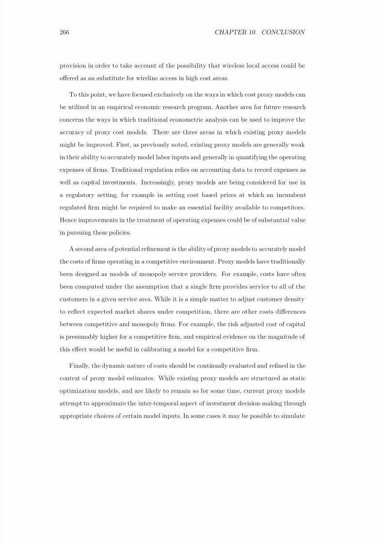
8/18/2019 Gasmi Cost Proxy Models
http://slidepdf.com/reader/full/gasmi-cost-proxy-models 266/318
266 CHAPTER 10. CONCLUSION
provision in order to take account of the possibility that wireless local access could be
offered as an substitute for wireline access in high cost areas.
To this point, we have focused exclusively on the ways in which cost proxy models can
be utilized in an empirical economic research program. Another area for future research
concerns the ways in which traditional econometric analysis can be used to improve the
accuracy of proxy cost models. There are three areas in which existing proxy models
might be improved. First, as previously noted, existing proxy models are generally weak
in their ability to accurately model labor inputs and generally in quantifying the operatingexpenses of firms. Traditional regulation relies on accounting data to record expenses as
well as capital investments. Increasingly, proxy models are being considered for use in
a regulatory setting, for example in setting cost based prices at which an incumbent
regulated firm might be required to make an essential facility available to competitors.
Hence improvements in the treatment of operating expenses could be of substantial value
in pursuing these policies.
A second area of potential refinement is the ability of proxy models to accurately model
the costs of firms operating in a competitive environment. Proxy models have traditionally
been designed as models of monopoly service providers. For example, costs have often
been computed under the assumption that a single firm provides service to all of the
customers in a given service area. While it is a simple matter to adjust customer density
to reflect expected market shares under competition, there are other costs differences
between competitive and monopoly firms. For example, the risk adjusted cost of capital
is presumably higher for a competitive firm, and empirical evidence on the magnitude of
this effect would be useful in calibrating a model for a competitive firm.
Finally, the dynamic nature of costs should be continually evaluated and refined in the
context of proxy model estimates. While existing proxy models are structured as static
optimization models, and are likely to remain so for some time, current proxy models
attempt to approximate the inter-temporal aspect of investment decision-making through
appropriate choices of certain model inputs. In some cases it may be possible to simulate

8/18/2019 Gasmi Cost Proxy Models
http://slidepdf.com/reader/full/gasmi-cost-proxy-models 267/318
10.3. SOME ISSUES NOT ADDRESSED IN OUR ANALYSIS AND SUGGESTIONS 267
a dynamic investment program more directly, and to incorporate this program into the
modeling process.

8/18/2019 Gasmi Cost Proxy Models
http://slidepdf.com/reader/full/gasmi-cost-proxy-models 268/318
268 NOTES
Notes
1We addressed these issues briefly in Chapter 1 and in somewhat more detail in Sections
2 and 3 of Chapter 3.
2For example, relatively crude proxies must be used to account for the effects of tech-
nological change. A measure of managerial effort as required in our approach would be
equally problematical.
3The model, LECOM, developed by Gabel and Kennet (1991) is described in detail in
Chapter 2. At that time Mark Kennet was not directly involved in the overall project other
than lending valuable assistance in the use of LECOM. Although we were not then aware
of it, a number of other computer based cost proxy models of local telecommunications
were simultaneously under development, though LECOM was the only publicly available
model.
4In other words, the regulator’s desire to minimize rents is not in conflict with the
desire to price efficiently in this case. Incomplete information requires a transfer under
the optimal mechanism, but the mechanism does not require a distortion in pricing beyond
that required by the Ramsey pricing rule.
5In order to run a large number of simulations over an extended period of time, we
created various batch files for automated operation of the model. The actual files used
to generate each of the simulations for Chapters 5 through 9 are provided on a CD
attachment to this volume.
6We note, however, that none of the more recently available models includes LECOM’s
ability to optimize switch locations.
7We note that even on the basis of initial cost, fiber is becoming increasingly compet-
itive with copper plant.
8An exception is our analysis of targeted entry in the universal service application,

8/18/2019 Gasmi Cost Proxy Models
http://slidepdf.com/reader/full/gasmi-cost-proxy-models 269/318
NOTES 269
where we briefly considered the assumption that the entrant possessed a superior tech-
nology to the incumbent. In addition, in Chapter 9 we considered the possibility that theentrant and incumbent might have incentives to choose different levels of effort.

8/18/2019 Gasmi Cost Proxy Models
http://slidepdf.com/reader/full/gasmi-cost-proxy-models 270/318
270 NOTES
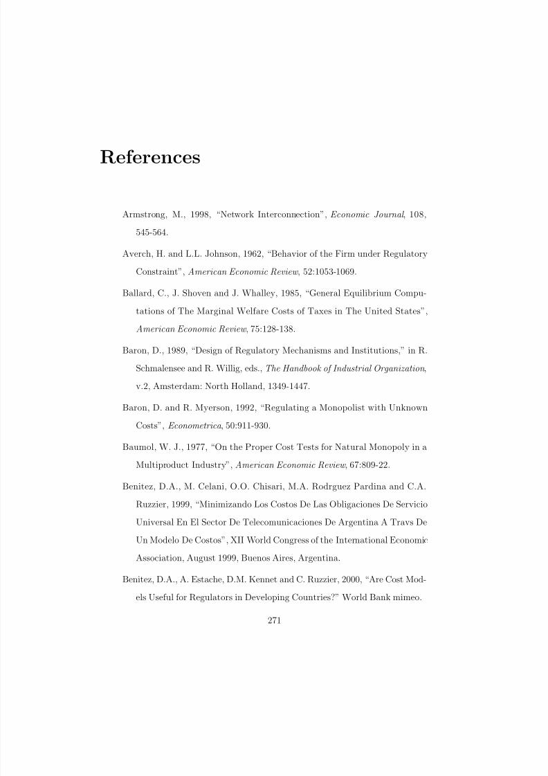
8/18/2019 Gasmi Cost Proxy Models
http://slidepdf.com/reader/full/gasmi-cost-proxy-models 271/318
References
Armstrong, M., 1998, “Network Interconnection”, Economic Journal , 108,
545-564.
Averch, H. and L.L. Johnson, 1962, “Behavior of the Firm under Regulatory
Constraint”, American Economic Review , 52:1053-1069.
Ballard, C., J. Shoven and J. Whalley, 1985, “General Equilibrium Compu-
tations of The Marginal Welfare Costs of Taxes in The United States”,
American Economic Review , 75:128-138.
Baron, D., 1989, “Design of Regulatory Mechanisms and Institutions,” in R.
Schmalensee and R. Willig, eds., The Handbook of Industrial Organization ,
v.2, Amsterdam: North Holland, 1349-1447.
Baron, D. and R. Myerson, 1992, “Regulating a Monopolist with Unknown
Costs”, Econometrica , 50:911-930.
Baumol, W. J., 1977, “On the Proper Cost Tests for Natural Monopoly in a
Multiproduct Industry”, American Economic Review , 67:809-22.
Benitez, D.A., M. Celani, O.O. Chisari, M.A. Rodrguez Pardina and C.A.
Ruzzier, 1999, “Minimizando Los Costos De Las Obligaciones De Servicio
Universal En El Sector De Telecomunicaciones De Argentina A Travs De
Un Modelo De Costos”, XII World Congress of the International Economic
Association, August 1999, Buenos Aires, Argentina.
Benitez, D.A., A. Estache, D.M. Kennet and C. Ruzzier, 2000, “Are Cost Mod-
els Useful for Regulators in Developing Countries?” World Bank mimeo.
271
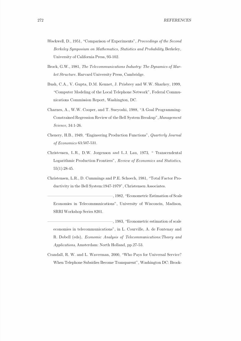
8/18/2019 Gasmi Cost Proxy Models
http://slidepdf.com/reader/full/gasmi-cost-proxy-models 272/318
272 REFERENCES
Blackwell, D., 1951, “Comparison of Experiments”, Proceedings of the Second
Berkeley Symposium on Mathematics, Statistics and Probability , Berkeley,University of California Press, 93-102.
Brock, G.W., 1981, The Telecommunications Industry: The Dynamics of Mar-
ket Structure . Harvard University Press, Cambridge.
Bush, C.A., V. Gupta, D.M. Kennet, J. Prisbrey and W.W. Sharkey, 1999,
“Computer Modeling of the Local Telephone Network”, Federal Commu-
nications Commission Report, Washington, DC.
Charnes, A., W.W. Cooper, and T. Sueyoshi, 1988, “A Goal Programming-
Constrained Regression Review of the Bell System Breakup”, Management
Science , 34:1-26.
Chenery, H.B., 1949, “Engineering Production Functions”, Quarterly Journal
of Economics 63:507-531.
Christensen, L.R., D.W. Jorgenson and L.J. Lau, 1973, “ Transcendental
Logarithmic Production Frontiers”, Review of Economics and Statistics ,
55(1):28-45.
Christensen, L.R., D. Cummings and P.E. Schoech, 1981, “Total Factor Pro-
ductivity in the Bell System:1947-1979”, Christensen Associates.
————————————————–, 1982, “Econometric Estimation of Scale
Economies in Telecommunications”, University of Wisconcin, Madison,
SRRI Workshop Series 8201.
————————————————–, 1983, “Econometric estimation of scale
economies in telecommunications”, in L. Courville, A. de Fontenay and
R. Dobell (eds), Economic Analysis of Telecommunications:Theory and
Applications , Amsterdam: North Holland, pp.27-53.
Crandall, R. W. and L. Waverman, 2000, “Who Pays for Universal Service?
When Telephone Subsidies Become Transparent”, Washington DC: Brook-
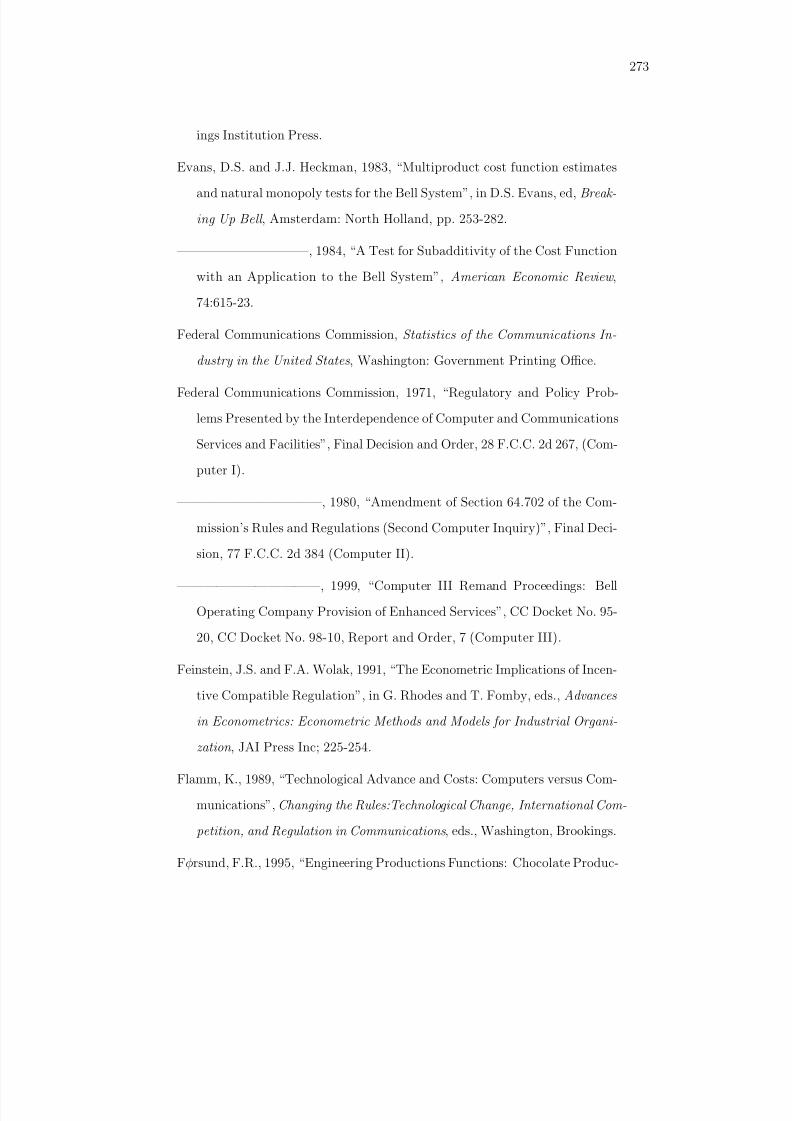
8/18/2019 Gasmi Cost Proxy Models
http://slidepdf.com/reader/full/gasmi-cost-proxy-models 273/318
273
ings Institution Press.
Evans, D.S. and J.J. Heckman, 1983, “Multiproduct cost function estimates
and natural monopoly tests for the Bell System”, in D.S. Evans, ed, Break-
ing Up Bell , Amsterdam: North Holland, pp. 253-282.
——————————, 1984, “A Test for Subadditivity of the Cost Function
with an Application to the Bell System”, American Economic Review ,
74:615-23.
Federal Communications Commission, Statistics of the Communications In-
dustry in the United States , Washington: Government Printing Office.
Federal Communications Commission, 1971, “Regulatory and Policy Prob-
lems Presented by the Interdependence of Computer and Communications
Services and Facilities”, Final Decision and Order, 28 F.C.C. 2d 267, (Com-
puter I).
———————————, 1980, “Amendment of Section 64.702 of the Com-
mission’s Rules and Regulations (Second Computer Inquiry)”, Final Deci-
sion, 77 F.C.C. 2d 384 (Computer II).
———————————, 1999, “Computer III Remand Proceedings: Bell
Operating Company Provision of Enhanced Services”, CC Docket No. 95-
20, CC Docket No. 98-10, Report and Order, 7 (Computer III).
Feinstein, J.S. and F.A. Wolak, 1991, “The Econometric Implications of Incen-
tive Compatible Regulation”, in G. Rhodes and T. Fomby, eds., Advances
in Econometrics: Econometric Methods and Models for Industrial Organi-
zation , JAI Press Inc; 225-254.
Flamm, K., 1989, “Technological Advance and Costs: Computers versus Com-
munications”, Changing the Rules:Technological Change, International Com-
petition, and Regulation in Communications , eds., Washington, Brookings.
Fφrsund, F.R., 1995, “Engineering Productions Functions: Chocolate Produc-
8/18/2019 Gasmi Cost Proxy Models
http://slidepdf.com/reader/full/gasmi-cost-proxy-models 274/318
274 REFERENCES
tion Revisited”, Mimeo, Department of Economics, University of Oslo.
Freidenfelds, J., 1978, “A Simple Model for Studying Feeder Capacity Expan-
sion”, Bell System Technical Journal , 57:807-824.
Frisch, R., 1935, “The Principle of Substitution. An Example of its Applica-
tion in The Chocolate Industry”. Nordisk Tidskrift for Teknisk Konomi
12-27.
Fuss, M. and L. Waverman, 1978, “Multi-product, multi-input cost functions
for a regulated utility: the case of telecommunications in Canada”, Work-
ing Paper 7810, Institute for Policy Analysis, University of Toronto.
Gabel, D. and D.M. Kennet, 1991, “Estimating the Cost Structure of the Lo-
cal Telephone Exchange Network”, National Regulatory Research Institute ,
Report 91-16, Colombus, Ohio.
————————–, 1994, “Economies of Scope in the Local Exchange Mar-ket,” Journal of Regulatory Economics , 6, 381-398.
Gasmi, F., M. Ivaldi and J.J. Laffont, 1994, “Rent extraction and incentives for
efficiency in recent regulatory proposals”, Journal of Regulatory Economics
6:151-176.
Gasmi, F., J.J. Laffont and W.W. Sharkey, 1997, “Incentive Regulation and
The Cost Structure of The Local Telephone Exchange Network”, Journal
of Regulatory Economics , 12:5-25.
————————————-, 1999a, “Empirical Evaluation of Regulatory Regimes
in Local Telecommunications Markets”, Journal of Economics & Manage-
ment Strategy , Vol.8 , 61-93.
————————————-, 1999b, “Competition, Universal Service and Telecom-
munications Policy in Developing Countries”, Information Economics and
Policy , 12(3):221-228.

8/18/2019 Gasmi Cost Proxy Models
http://slidepdf.com/reader/full/gasmi-cost-proxy-models 275/318
275
————————————-, 1999c, “The Natural Monopoly Test Reconsid-
ered: An Engineering Process-Based Approach to Empirical Analysis inTelecommunications”. Forthcoming in International Journal of Industrial
Organization .
————————————-, 2001, “Provision of Universal Service for Telecom-
munications in Densely Populated Developing Countries”. Forthcoming in
Telecommunications Reform in India . Quorum Imprint, Greenwood.
Gasmi, F., J.J. Laffont and Q. Vuong, 1992, “Econometric Analysis of Col-lusive Behavior in a Soft-Drink Market”, Journal of Economics and Man-
agement Strategy , Vol 1(2), 277-311.
Gibbard, A. , 1973, “Manipulation of Voting Schemes: A General Result”
Econometrica , 41, 587-601.
Green, J. and J.J. Laffont, 1979, Incentives in Public Decision Making . Ams-
terdam: North-Holland.
————————–, 1977, “Characterization of Satisfactory Mechanisms for
the Revelation of Preferences for Public goods”, Econometrica , 45, 427-438.
Green, W.H., 2000, Econometric Analysis . Prentice Hall International, Inc.
Griffen, J.M., 1972, “The Process Analysis Alternative to Statistical Cost
Functions”, American Economic Review 62:46-56.
Griffin, J.M., 1977, “The Econometrics of Joint Production: Another Ap-
proach”, Bell Journal of Economics , 8:112-27.
————-, 1977, “Long-run Production Modeling with Pseudo Data: Electric
Power Generation”, Bell Journal of Economics , 8:112-27.
Hausman, J. and J. Poterba, 1987, “Household Behavior and The tax Reform
Act of 1986”, The Journal of Economic Perspectives , 1: 101-119.
Hurwicz, L., 1960, “Optimality and Informational Efficiency in Resource Allo-
cation Process” in Arrow, Karkin and Suppes, eds, Mathematical Methods
8/18/2019 Gasmi Cost Proxy Models
http://slidepdf.com/reader/full/gasmi-cost-proxy-models 276/318
276 REFERENCES
in the Social Sciences , Stanford University Press.
Kahn, A.E., 1970, The Economics of Regulation: Principles and Institutions ,
vol. 1 and 2 John Wiley & Sons, New York.
Laffont, J.J., 1994, “The New Economics of Regulation Ten Years After”,
Econometrica , 62, 507-537.
————-, 1996, “Industrial Policy and Politics”, International Journal of
Industrial Organization 14, 1-27.
Laffont, J.J. and M. Matoussi, 1995, “Moral Hazard, Financial Constraints
and Sharecropping in El Oulja”, Review of Economic Studies , 62, 381-399.
Laffont, J.J. and M. Meleu, 1999, “Separation of Powers and Development”.
Forthcoming in Journal of Economic Development .
Laffont, J.J., H. Ossard and Q. Vuong, 1995, “Econometrics of First-Price
Auctions”, Econometrica , 63, 953-980.
Laffont, J.J., P. Rey and J. Tirole, (1998a), “Network Competition: I. Overview
and Non-discrimination Pricing”, Rand Journal of Economics , 29, 1-37.
———————————-, (1998b), “Network Competition: II. Price Discrim-
ination”, Rand Journal of Economics , 29, 38-56.
Laffont, J.J., and J. Tirole, 1986, “Using Cost Information to Regulate Firms”,
Journal of Political Economy , 94, 1-49.
—————————-, 1993, A Theory of Incentives in Procurement and Reg-
ulation , MIT Press, Cambridge.
—————————-, 2000, Competition in Telecommunications , MIT Press,
Cambridge.
Legette III, James A., 1985, Natural Monopoly in the Telecommunication In-
dustry: The Case of Local Service , Unpublished Ph.D. Dissertation, Uni-
versity of South Carolina.
8/18/2019 Gasmi Cost Proxy Models
http://slidepdf.com/reader/full/gasmi-cost-proxy-models 277/318
277
Littlechild, S.C. 1983, “Regulation of British Telecom’s Profitability”. Report
to the Secretary of State, Department of Industry, London.
Loeb, M., and W. Magat, 1979, “A Decentralized Method of Utility Regula-
tion”, Journal of Law and Economics , 22:399-404.
Maher, M.E., 1999, “Access Costs and Entry in the Local Telecommunica-
tions Network: A Case for De-averaged Rates”, International Journal of
Industrial Organization , 17:593-609.
Manne, A. 1958, “A Linear Programming Model of the U.S. Petroleum Refin-
ing Industry”, Econometrica 26:67-106.
Mitchell, B.M., 1990, “Incremental costs of telephone access and local use”,
Rand Report R- 3909–ICTF.
Mundlak, Y., 1978, “On the Pooling of Time Series and Cross Section Data”,
Econometrica , 46:69-85.
Myerson, R., 1979, “Incentive Compatibility and the Bargaining Problem”,
Econometrica , 47, 61-74.
———–, 1981, “Optimal Auction Design”, Mathematics of Operations Re-
search 6, 58-73.
National Telecommunication and Information Administration, 1988, NTIA
Telecom 2000: Charting the Course for A New Century , Washington: US
Dept. of Commerce.
Nelder, J., A. and R. Mead, 1965, “A Simplex Method for Function Minimiza-
tion”, Computer Journal , 7:308-313.
New England Telephone, 1986, Massachusetts Incremental Cost Study, Mas-
sachusetts Department of Public Utilities Docket, 86-33.
Palmer, K., 1992, “A Test for Cross Subsidies in Local Telephone Rates: Do
Business Customers Subsidize Residential Customers?”, Rand Journal of
Economics , vol.23, no 3.
8/18/2019 Gasmi Cost Proxy Models
http://slidepdf.com/reader/full/gasmi-cost-proxy-models 278/318
278 REFERENCES
Panzar, J.C., 1989, “Technological Determinants of Firm and Industry Struc-
ture”, in R. Schmalensee and R. Willig (eds), Handbook of Industrial Or-ganization , vol. I. (Elsevier Science Publishing), 3-59.
Press, W.H., B.P. Flannery, S.A. Jeukolsky and W.T. Vetterling, 1986, Nu-
mental Recipes: The Art of Scientific Computing . Cambridge University
Press, Cambridge, MA.
Rey, R.F. (Technical Editor), 1984, Engineering and Operations in the Bell
System . AT & T Bell Laboratories, Murray Hill, NJ.
Schmalensee, R., 1989, “Good regulatory regimes”, Rand Journal of Eco-
nomics 20:417-436.
Sharkey, W.W., 1982, The Theory of Natural Monopoly . Cambridge University
Press.
————-, 2001, “Representation of Technology and Production”, in Cave,
M, Majumdar, S. and I. Vogelsang (eds), Handbook of Telecommunications
Economics , Chapter 6. Amsterdam: Elsevier Science, NV.
Shin, R.T. and J.S., Ying, 1992, “Unnatural Monopolies in Local Telephone”,
Rand Journal of Economics 23 (2):171-183.
Shleifer, A., 1985, “A Theory of Yardstick Competition”, Rand Journal of
Economics , 16:319-327.
Smith, V.L., 1957, “Engineering Data and Statistical Techniques in the Anal-
ysis of Production and Technological Change: Fuel Requirements in the
Trucking Industry”, Econometrica 25:281-301.
Soares, J. F., 1998, Teoria E Prtica De Subsidiao Cruzada - Aplicao A Uma
Rede Local De Telecomunicaes Portuguesa (Theory and Practice of Cross-
Subsidy - Application to a Portuguese Local Telecommunications Net-
work). Unpublished Ph.D. dissertation, Instituto Superior De Economia
E Gesto Da Universidade Tcnica De Lisboa.
8/18/2019 Gasmi Cost Proxy Models
http://slidepdf.com/reader/full/gasmi-cost-proxy-models 279/318
279
Taylor, L.D., 1994, Telecommunications Demand in Theory and Practice .
Kluwer Academic Publishers.
Temin, P., 1990, “Cross-Subsidies in the Telephone Network after Divestiture”,
Journal of Regulatory Economics , 2:349-362.
Varian, H., 1992, Microeconomic Analysis , Norton & Company, New York.
von Weizscker, C.C., 1980, “A Welfare Analysis of Barriers to Entry”, Bell
Journal of Economics 11(2): 399-420.
Wimmer, B. and G. L. Rosston,2000 “The ‘State‘ of Universal Service”. In-
formation Economics and Policy , 12(3), 2000:pp. 261-283.
—————————,2000, “Winners and Losers from the Universal Service
Subsidy Battle” in Compaine, B. and Vogelsang, I. (eds), The Internet
Upheaval, raising questions, seeking answers in communications policy:
Selected Papers from the Telecommunications Policy Research Conference .
MIT Press, Cambridge MA.
—————————,2000, “From C-to-Shining-C: Competition and Cross Sub-
sidy in Telecommunications” in Compaine, B. and Greenstein S. (eds),
Selected Papers from the Telecommunications Policy Research Conference ,
(fothcoming). MIT Press, Cambridge.
Wolak, F.A., 1994, “An Econometric Analysis of the Asymmetric Information,
Regulator-Utility Interaction”, Annales d’Economie et de Statistique , 34,
13-69.
Wilson, R., 1989, “Efficient and Competitive Rationing”, Econometrica , 57,
1-40.
Wunsch P., 1994, “Estimating menus of linear contracts for mass transit
firms”, Mimeo, CORE, Louvain-La-Neuve, Belgium.

8/18/2019 Gasmi Cost Proxy Models
http://slidepdf.com/reader/full/gasmi-cost-proxy-models 280/318
280 REFERENCES

8/18/2019 Gasmi Cost Proxy Models
http://slidepdf.com/reader/full/gasmi-cost-proxy-models 281/318
Appendix A
A.1 The Natural Monopoly Test (Chapter 5)
This section of the appendix presents the translog estimation of the various cost functions
used in Chapter 5. The values of the estimated parameters are rounded to the second
decimal.1
• Usage as output (Section 5.4.1)
LogC (PK , PL , Q) = 16.96 + 0.44LogPK + 0.44LogPL+0.15LogQ + 0.11(LogPK )2 + 0.12(LogPL)2
+0.02(LogQ)2 − 0.18LogPKLogPL−0.01LogPKLogQ + 0.01LogQLogPL
(A.1)
• Access as output2
- Monopoly:
LogC M
(PK , PL , N ) = 18.64 + 0.52LogPK + 0.31LogPL − 1.20LogN +0.12(LogPK )2 + 0.12(LogPL)2 + 0.09(LogN )2
−0.18LogPKLogPL − 0.01LogPKLogN +0.01LogNLogPL
(A.2)
- Duopoly:
. Uniform entry without accounting for interconnection costs:
LogC DU (PK , PL , N i) = 18.64 + 0.52LogPK + 0.31LogPL − 1.20LogN i+0.12(LogPK )2 + 0.12(LogPL)2 + 0.09(LogN i)2
−0.18LogPKLogPL − 0.01LogPKLogN i + 0.01LogN iLogPL(A.3)
281

8/18/2019 Gasmi Cost Proxy Models
http://slidepdf.com/reader/full/gasmi-cost-proxy-models 282/318
282 APPENDIX A
. Uniform entry with interconnection costs accounted for:
LogC D
U (PK , PL , N i) = 18.64 + 0.52LogPK + 0.31LogPL−1.20LogN i + 0.12(LogPK )2 + 0.12(LogPL)2 + 0.09(LogN i)2
−0.18LogPKLogPL − 0.01LogPKLogN i + 0.01LogN iLogPL(A.4)
. Targeted entry without accounting for interconnection cost:
LogC DT (PK , L , N i, Ai) = 14.24 + 0.49LogPK +0.35LogPL − 0.78LogN i + 0.73LogAi + 0.12(LogPK )2
+0.12(LogPL)2 + 0.09(LogN i)2 + 0.09(LogAi)2
−0.18LogPKLogPL − 0.01LogPKLogN i + 0.01LogPKLogAi
+0.01LogN iLogPL − 0.01LogAiLogPL − 0.10LogN iLogAi
(A.5)
where Ai ≡ 57.39 × N i
N i + N j, i, j = 1, 2 , i = j
. Targeted entry with interconnection costs accounted for:
LogC DT (PK , PL , N i, Ai) = 14.24 + 0.49LogPK +0.35LogPL − 0.78LogN i + 0.73LogAi + 0.12(LogPK )2
+0.12(LogPL)2 + 0.09(LogN i)2 + 0.09(LogAi)2
−0.18LogPKLogPL − 0.01LogPKLogN i + 0.01LogPKLogAi
+0.01LogN iLogPL − 0.01LogAiLogPL − 0.10LogN iLogAi
(A.6)
where Ai is a defined above.
A.2 Optimal Regulation of a Natural Monopoly(Chapter 6)
Recall from the text that we assumed that the technological efficiency parameter β had
a uniform distribution with support [0.5; 1.5]. Asymmetric information allows the firm toenjoy some rent and we have explored empirically the effect of improving the regulator’s
information by tightening the support of the uniform distribution and also by using the
normal distribution instead of the uniform. Table A.1 presents the level of rent for each
β and expected social welfare achieved in those experiments. In this table, the index “1”
refers to our base case, i.e., the calculations that make use of the uniform distribution
with support [0.5; 1.5], the index “2” refers to a case where the uniform distribution is
still used but its support tightened to [0.7; 1.3] and the index “3” corresponds to a case
where the normal distribution with support [0.5; 1.5] is used.
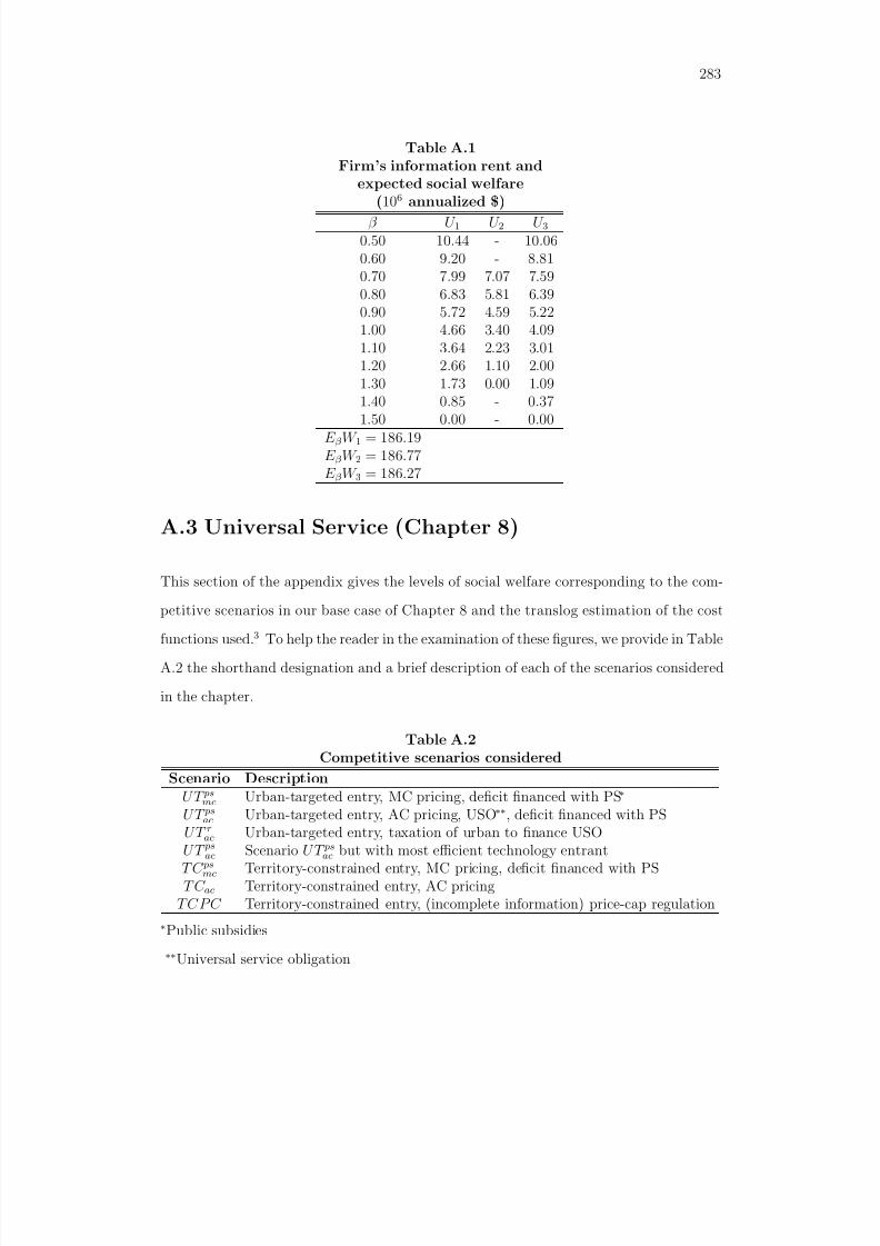
8/18/2019 Gasmi Cost Proxy Models
http://slidepdf.com/reader/full/gasmi-cost-proxy-models 283/318
283
Table A.1Firm’s information rent and
expected social welfare(106 annualized $)
β U 1 U 2 U 30.50 10.44 - 10.060.60 9.20 - 8.810.70 7.99 7.07 7.590.80 6.83 5.81 6.390.90 5.72 4.59 5.221.00 4.66 3.40 4.091.10 3.64 2.23 3.01
1.20 2.66 1.10 2.001.30 1.73 0.00 1.091.40 0.85 - 0.371.50 0.00 - 0.00
E β W 1 = 186.19E β W 2 = 186.77E β W 3 = 186.27
A.3 Universal Service (Chapter 8)
This section of the appendix gives the levels of social welfare corresponding to the com-
petitive scenarios in our base case of Chapter 8 and the translog estimation of the cost
functions used.3 To help the reader in the examination of these figures, we provide in Table
A.2 the shorthand designation and a brief description of each of the scenarios considered
in the chapter.
Table A.2Competitive scenarios considered
Scenario DescriptionU T ps
mc Urban-targeted entry, MC pricing, deficit financed with PS∗
U T psac Urban-targeted entry, AC pricing, USO∗∗, deficit financed with PS
UT τ ac Urban-targeted entry, taxation of urban to finance USO
U T psac Scenario U T ps
ac but with most efficient technology entrantT C ps
mc Territory-constrained entry, MC pricing, deficit financed with PST C ac Territory-constrained entry, AC pricing
T C P C Territory-constrained entry, (incomplete information) price-cap regulation
∗Public subsidies
∗∗Universal service obligation
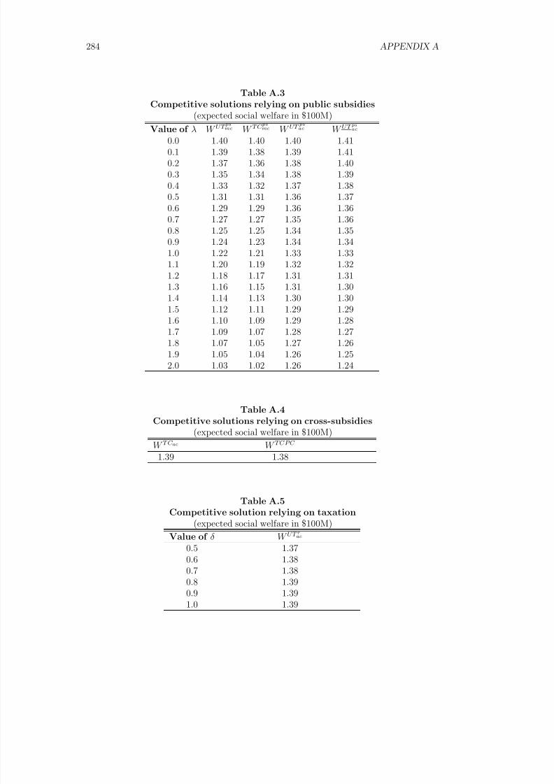
8/18/2019 Gasmi Cost Proxy Models
http://slidepdf.com/reader/full/gasmi-cost-proxy-models 284/318
284 APPENDIX A
Table A.3Competitive solutions relying on public subsidies
(expected social welfare in $100M)Value of λ W U T
psmc W T C
psmc W UT
psac W U T psac
0.0 1.40 1.40 1.40 1.410.1 1.39 1.38 1.39 1.410.2 1.37 1.36 1.38 1.400.3 1.35 1.34 1.38 1.390.4 1.33 1.32 1.37 1.380.5 1.31 1.31 1.36 1.370.6 1.29 1.29 1.36 1.360.7 1.27 1.27 1.35 1.36
0.8 1.25 1.25 1.34 1.350.9 1.24 1.23 1.34 1.341.0 1.22 1.21 1.33 1.331.1 1.20 1.19 1.32 1.321.2 1.18 1.17 1.31 1.311.3 1.16 1.15 1.31 1.301.4 1.14 1.13 1.30 1.301.5 1.12 1.11 1.29 1.291.6 1.10 1.09 1.29 1.281.7 1.09 1.07 1.28 1.27
1.8 1.07 1.05 1.27 1.261.9 1.05 1.04 1.26 1.252.0 1.03 1.02 1.26 1.24
Table A.4Competitive solutions relying on cross-subsidies
(expected social welfare in $100M)
W T C ac W T C P C
1.39 1.38
Table A.5Competitive solution relying on taxation
(expected social welfare in $100M)
Value of δ W U T τ ac
0.5 1.370.6 1.380.7 1.380.8 1.390.9 1.391.0 1.39

8/18/2019 Gasmi Cost Proxy Models
http://slidepdf.com/reader/full/gasmi-cost-proxy-models 285/318
285
- Cost function of an incumbent serving the rural area while facing entry in the urban
area:
LogC U T 1 (PK , PL , Q11, Q21) = 16.35 + 0.47LogPK + 0.42LogPL
−0.01LogQ11 + 0.01LogQ21 + 0.12(LogPK )2
+0.12(LogPL)2 + 0.01(LogQ11)2 + 0.02(LogQ21)2
−0.018LogPKLogPL − 0.002LogPKLogQ11
−0.001LogPKLogQ21 + 0.001LogQ11LogPL+0.002LogQ21LogPL − 0.002LogQ11LogQ21
- Cost function of an entrant serving half of the urban area only:
LogC U T 2 (PK , PL , Q12) = 15.50 + 0.45LogPK + 0.43LogPL
+0.05LogQ12 + 0.12(LogPK )2 + 0.12(LogPL)2
+0.03(LogQ12)2 − 0.18LogPKLogPL−0.01LogPKLogQ12 + 0.004LogQ12LogPL
- Cost function of an entrant ( j = 2) and an incumbent ( j = 1) serving half of both
the urban and the rural areas:
LogC T C j (PK , PL , Q1 j, Q2 j) = 16.03 + 0.46LogPK + 0.42LogPL
−0.02LogQ1 j + 0.02LogQ2 j + 0.12(LogPK )2
+0.12(LogPL)2 + 0.01(LogQ1 j)2 + 0.02(LogQ2 j)2
−0.18LogPKLogPL + 0.01LogPKLogQ1 j
−0.01LogPKLogQ2 j − 0.003LogQ1 jLogPL
+0.01LogQ2 jLogPL + 0.001LogQ1 jLogQ2 j
A.4 Strategic Cross-Subsidies and Vertical Integration(Chapter 9)
This section of the appendix presents tables that complement the discussion of the em-
pirical results in Chapter 9 and the quadratic estimations of the cost functions used in
that chapter.
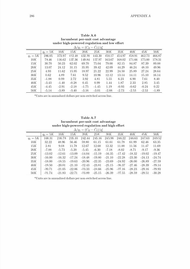
8/18/2019 Gasmi Cost Proxy Models
http://slidepdf.com/reader/full/gasmi-cost-proxy-models 286/318
286 APPENDIX A
Table A.6
Incumbent per-unit cost advantageunder high-powered regulation and low effort
∆/q 1 = (C E − C I )/q ∗1q 2 = 5K 10K 15K 20K 25K 30K 35K 40K 45K 50K
q 1 = 5K 286.05 373.97 412.48 432.20 443.30 450.17 454.97 458.91 462.73 466.8710K 78.46 116.62 137.36 149.84 157.97 163.67 168.02 171.66 175.00 178.3115K 30.70 50.23 62.02 69.70 75.04 79.00 82.15 84.87 87.39 89.8820K 13.07 24.12 31.15 35.95 39.42 42.09 44.29 46.24 48.10 49.9625K 4.93 11.62 15.95 18.97 21.22 22.99 24.50 25.89 27.24 28.6430K 0.62 4.89 7.61 9.52 10.96 12.12 13.14 14.11 15.10 16.14
35K -1.88 0.99 2.72 3.92 4.81 5.55 6.23 6.90 7.61 8.4040K -3.43 -1.40 -0.28 0.45 0.99 1.44 1.87 2.33 2.85 3.4545K -4.45 -2.91 -2.18 -1.75 -1.45 1.19 -0.93 -0.62 -0.24 0.2250K -5.14 -3.89 -3.40 -3.16 -3.01 -2.88 -2.73 -2.53 -2.53 -1.89
*Units are in annualized dollars per non-switched access line.
Table A.7Incumbent per-unit cost advantageunder high-powered regulation and high effort
∆/q 1 = (C E − C I )/q ∗1q 2 = 5K 10K 15K 20K 25K 30K 35K 40K 45K 50K
q 1 = 5K 168.31 216.78 235.10 242.44 245.16 245.98 246.22 246.63 247.63 249.5210K 32.22 48.96 56.46 59.80 61.15 61.61 61.78 61.99 62.46 63.3515K 2.81 9.08 11.78 12.67 12.68 12.32 11.88 11.56 11.47 11.6920K -7.88 -5.73 -5.20 -5.45 -6.30 -7.18 -8.02 -8.71 -9.17 -9.3625K -13.02 -12.61 -13.09 -14.04 -15.19 -16.35 -17.42 -18.32 -19.02 -19.47
30K -16.00 -16.32 -17.24 -18.48 -19.80 -21.10 -22.28 -23.30 -24.13 -24.7435K -18.00 -18.55 -19.63 -20.96 -22.35 -23.69 -24.92 -26.00 -26.89 -27.5940K -19.50 -20.01 -21.10 -22.43 -23.81 -25.15 -26.37 -27.46 -28.39 -29.1445K -20.71 -21.05 -22.06 -23.33 -24.66 -25.96 -27.16 -28.23 -29.16 -29.9350K -21.74 -21.83 -22.71 -23.89 -25.15 -26.39 -27.55 -28.59 -29.51 -30.28
*Units are in annualized dollars per non-switched access line.
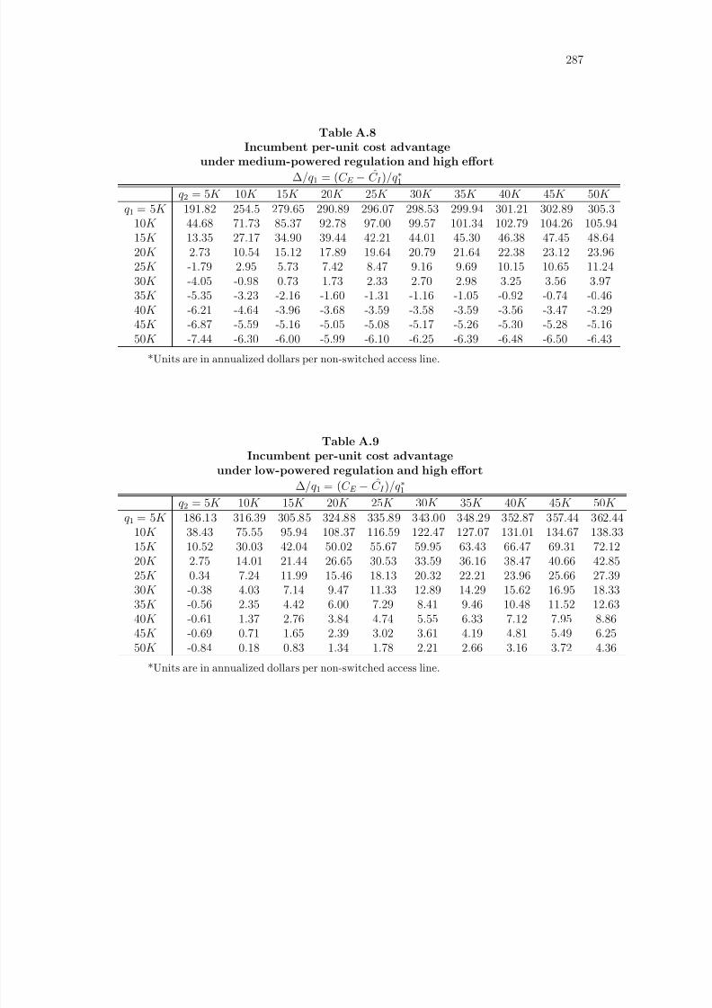
8/18/2019 Gasmi Cost Proxy Models
http://slidepdf.com/reader/full/gasmi-cost-proxy-models 287/318
287
Table A.8
Incumbent per-unit cost advantageunder medium-powered regulation and high effort
∆/q 1 = (C E − C I )/q ∗1q 2 = 5K 10K 15K 20K 25K 30K 35K 40K 45K 50K
q 1 = 5K 191.82 254.5 279.65 290.89 296.07 298.53 299.94 301.21 302.89 305.310K 44.68 71.73 85.37 92.78 97.00 99.57 101.34 102.79 104.26 105.9415K 13.35 27.17 34.90 39.44 42.21 44.01 45.30 46.38 47.45 48.6420K 2.73 10.54 15.12 17.89 19.64 20.79 21.64 22.38 23.12 23.9625K -1.79 2.95 5.73 7.42 8.47 9.16 9.69 10.15 10.65 11.2430K -4.05 -0.98 0.73 1.73 2.33 2.70 2.98 3.25 3.56 3.97
35K -5.35 -3.23 -2.16 -1.60 -1.31 -1.16 -1.05 -0.92 -0.74 -0.4640K -6.21 -4.64 -3.96 -3.68 -3.59 -3.58 -3.59 -3.56 -3.47 -3.2945K -6.87 -5.59 -5.16 -5.05 -5.08 -5.17 -5.26 -5.30 -5.28 -5.1650K -7.44 -6.30 -6.00 -5.99 -6.10 -6.25 -6.39 -6.48 -6.50 -6.43
*Units are in annualized dollars per non-switched access line.
Table A.9Incumbent per-unit cost advantageunder low-powered regulation and high effort
∆/q 1 = (C E − C I )/q ∗1q 2 = 5K 10K 15K 20K 25K 30K 35K 40K 45K 50K
q 1 = 5K 186.13 316.39 305.85 324.88 335.89 343.00 348.29 352.87 357.44 362.4410K 38.43 75.55 95.94 108.37 116.59 122.47 127.07 131.01 134.67 138.3315K 10.52 30.03 42.04 50.02 55.67 59.95 63.43 66.47 69.31 72.1220K 2.75 14.01 21.44 26.65 30.53 33.59 36.16 38.47 40.66 42.8525K 0.34 7.24 11.99 15.46 18.13 20.32 22.21 23.96 25.66 27.39
30K -0.38 4.03 7.14 9.47 11.33 12.89 14.29 15.62 16.95 18.3335K -0.56 2.35 4.42 6.00 7.29 8.41 9.46 10.48 11.52 12.6340K -0.61 1.37 2.76 3.84 4.74 5.55 6.33 7.12 7.95 8.8645K -0.69 0.71 1.65 2.39 3.02 3.61 4.19 4.81 5.49 6.2550K -0.84 0.18 0.83 1.34 1.78 2.21 2.66 3.16 3.72 4.36
*Units are in annualized dollars per non-switched access line.
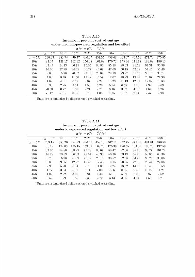
8/18/2019 Gasmi Cost Proxy Models
http://slidepdf.com/reader/full/gasmi-cost-proxy-models 288/318
288 APPENDIX A
Table A.10
Incumbent per-unit cost advantageunder medium-powered regulation and low effort
∆/q 1 = (C E − C I )/q ∗1q 2 = 5K 10K 15K 20K 25K 30K 35K 40K 45K 50K
q 1 = 5K 290.23 380.24 419.77 440.07 451.55 458.68 463.67 467.76 471.70 475.9510K 81.37 121.17 142.92 156.08 164.68 170.72 175.34 179.18 182.68 186.1315K 33.47 54.13 66.75 75.05 80.86 85.18 88.63 91.59 94.31 96.9620K 16.00 27.78 34.45 40.77 44.67 47.69 50.18 52.38 54.45 56.4925K 8.08 15.20 20.02 23.48 26.09 28.19 29.97 31.60 33.16 34.7430K 4.00 8.48 11.56 13.82 15.57 17.02 18.29 19.49 20.67 21.90
35K 1.69 4.61 6.59 8.07 9.24 10.23 11.13 12.01 12.92 13.8840K 0.30 2.25 3.54 4.50 5.26 5.94 6.58 7.23 7.92 8.6945K -0.58 0.77 1.60 2.21 2.71 3.16 3.62 4.10 4.64 5.2650K -1.17 -0.19 0.35 0.73 1.05 1.35 1.67 2.04 2.47 2.98
*Units are in annualized dollars per non-switched access line.
Table A.11Incumbent per-unit cost advantageunder low-powered regulation and low effort
∆/q 1 = (C E − C I )/q ∗1q 2 = 5K 10K 15K 20K 25K 30K 35K 40K 45K 50K
q 1 = 5K 289.15 383.20 424.93 446.65 459.18 467.11 472.75 477.40 481.81 486.5010K 80.19 122.03 145.15 159.32 168.70 175.39 180.55 184.86 188.78 192.5915K 33.05 54.80 68.29 77.28 83.67 88.47 92.36 95.70 98.77 101.7420K 16.22 28.59 36.83 42.64 46.96 50.36 53.19 55.70 58.05 60.3625K 8.78 16.20 21.39 25.19 28.13 30.52 32.58 34.45 36.25 38.06
30K 5.03 9.65 12.97 15.48 17.48 19.15 20.65 22.05 23.44 24.8635K 2.98 5.90 8.04 9.70 11.06 12.24 13.32 14.38 15.45 16.5840K 1.77 3.64 5.02 6.11 7.03 7.86 8.65 9.45 10.29 11.2045K 1.02 2.22 3.10 3.81 4.43 5.01 5.59 6.20 6.87 7.6250K 0.52 1.29 1.85 2.30 2.72 3.13 3.56 4.04 4.59 5.21
*Units are in annualized dollars per non-switched access line.
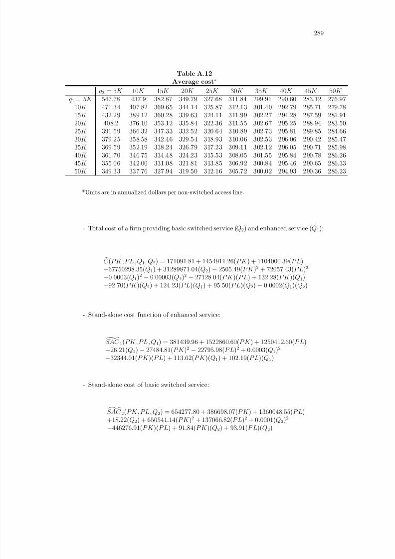
8/18/2019 Gasmi Cost Proxy Models
http://slidepdf.com/reader/full/gasmi-cost-proxy-models 289/318
289
Table A.12
Average cost∗q 2 = 5K 10K 15K 20K 25K 30K 35K 40K 45K 50K
q 1 = 5K 547.78 437.9 382.87 349.79 327.68 311.84 299.91 290.60 283.12 276.9710K 471.34 407.82 369.65 344.14 325.87 312.13 301.40 292.79 285.71 279.7815K 432.29 389.12 360.28 339.63 324.11 311.99 302.27 294.28 287.59 281.9120K 408.2 376.10 353.12 335.84 322.36 311.55 302.67 295.25 288.94 283.5025K 391.59 366.32 347.33 332.52 320.64 310.89 302.73 295.81 289.85 284.6630K 379.25 358.58 342.46 329.54 318.93 310.06 302.53 296.06 290.42 285.4735K 369.59 352.19 338.24 326.79 317.23 309.11 302.12 296.05 290.71 285.9840K 361.70 346.75 334.48 324.23 315.53 308.05 301.55 295.84 290.78 286.26
45K 355.06 342.00 331.08 321.81 313.85 306.92 300.84 295.46 290.65 286.3350K 349.33 337.76 327.94 319.50 312.16 305.72 300.02 294.93 290.36 286.23
*Units are in annualized dollars per non-switched access line.
- Total cost of a firm providing basic switched service (Q2) and enhanced service (Q1):
C (PK , PL , Q1, Q2) = 171091.81 + 1454911.26(P K ) + 1104000.39(P L)+67750298.35(Q1) + 31289871.04(Q2) − 2505.49(P K )2 + 72057.43(P L)2
−0.0003(Q1)2 − 0.00003(Q2)2 − 27128.04(P K )(P L) + 132.28(P K )(Q1)+92.70(P K )(Q2) + 124.23(P L)(Q1) + 95.50(P L)(Q2) − 0.0002(Q1)(Q2)
- Stand-alone cost function of enhanced service:
SAC 1(PK , PL , Q1) = 381439.96 + 1522860.60(P K ) + 1250412.60(P L)+26.21(Q1) − 27484.81(P K )2 − 22795.98(P L)2 + 0.0003(Q1)2
+32344.01(P K )(P L) + 113.62(P K )(Q1) + 102.19(P L)(Q1)
- Stand-alone cost of basic switched service:
SAC 2(PK , PL , Q2) = 654277.80 + 386698.07(P K ) + 1360048.55(P L)+18.22(Q2) + 650541.14(P K )2 + 137066.82(P L)2 + 0.0001(Q2)2
−446276.91(P K )(P L) + 91.84(P K )(Q2) + 93.91(P L)(Q2)
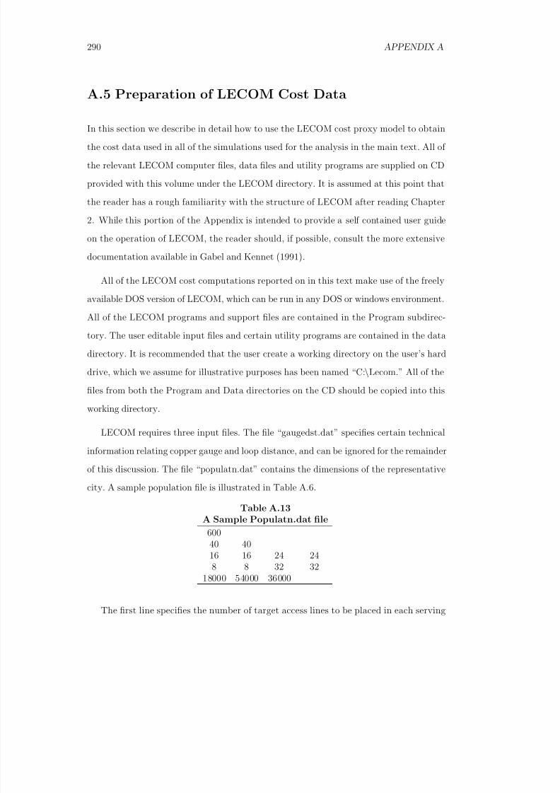
8/18/2019 Gasmi Cost Proxy Models
http://slidepdf.com/reader/full/gasmi-cost-proxy-models 290/318
290 APPENDIX A
A.5 Preparation of LECOM Cost Data
In this section we describe in detail how to use the LECOM cost proxy model to obtain
the cost data used in all of the simulations used for the analysis in the main text. All of
the relevant LECOM computer files, data files and utility programs are supplied on CD
provided with this volume under the LECOM directory. It is assumed at this point that
the reader has a rough familiarity with the structure of LECOM after reading Chapter
2. While this portion of the Appendix is intended to provide a self contained user guide
on the operation of LECOM, the reader should, if possible, consult the more extensive
documentation available in Gabel and Kennet (1991).
All of the LECOM cost computations reported on in this text make use of the freely
available DOS version of LECOM, which can be run in any DOS or windows environment.
All of the LECOM programs and support files are contained in the Program subdirec-
tory. The user editable input files and certain utility programs are contained in the data
directory. It is recommended that the user create a working directory on the user’s hard
drive, which we assume for illustrative purposes has been named “C:\Lecom.” All of the
files from both the Program and Data directories on the CD should be copied into this
working directory.
LECOM requires three input files. The file “gaugedst.dat” specifies certain technical
information relating copper gauge and loop distance, and can be ignored for the remainder
of this discussion. The file “populatn.dat” contains the dimensions of the representative
city. A sample population file is illustrated in Table A.6.
Table A.13A Sample Populatn.dat file
60040 4016 16 24 248 8 32 32
18000 54000 36000
The first line specifies the number of target access lines to be placed in each serving

8/18/2019 Gasmi Cost Proxy Models
http://slidepdf.com/reader/full/gasmi-cost-proxy-models 291/318
291
area. The next line gives the coordinates of the Northeast corner of the region under
study, measured in thousands of feet from the Southwest corner which is assumed to beat the origin. The next two lines give the Southwest and Northeast coordinates of the
central business District and the Mixed commercial and residential district respectively.
The last line gives the line counts to be placed in the central, mixed and residential
districts respectively.
The file “dvariabl.dat” specifies the remaining user inputs, which most significantly
for our purposes contain the input data for usage demands per access line in each citydistrict and input values for the price of capital and price of labor. Various other input
prices and algorithm control parameters are also specified in this file. A representative
dvariabl.dat file is illustrated in Table A.2.

8/18/2019 Gasmi Cost Proxy Models
http://slidepdf.com/reader/full/gasmi-cost-proxy-models 292/318
292 APPENDIX A
Table A.14A Sample Dvariabl.dat file
0.31300000000 * ac211 = carrying charge for land0.32690000000 * ac212 = carrying charge for buildings0.30140000000 * ac22157 = carrying charge for circuit0.37530000000 * acess = carrying charge for analog switches0.28080000000 * ac244 = carrying charge for conduit0.28120000000 * ac2422 = carrying charge for underground cable0.31660000000 * ac2423 = carrying charge for buried cable0.31660000000 * ac815 = carrying charge for underground fiber0.34310000000 * ac845 = carrying charge for buried fiber0.5000 * ccs per res line = ccs per residential customer
0.5000 * ccs per med line = ccs per medium density customer0.5000 * ccs per bus line = ccs per business customer0.90000000000 * perund bus = fraction of cable underground, business0.50000000000 * perund med = fraction of cable underground, mixed0.35000000000 * perund res = fraction of cable underground, residential0.068 * perpl[1] = fraction private lines for residential0.075 * perpl[2] = fraction private lines for mixed customers0.11 * perpl[3] = fraction private lines for business0.45000000000 * plcost = cost markup fraction for private lines0.94 * tollper = percentage toll traffic
0.4 * pltollper = private line percentage toll traffic1.68244500000 * f1526 =fixed investment per foot for UG 26 gauge cable1.91939600000 * f1524 = fixed investment per foot for UG 24 gauge cable1.74269200000 * f1522 = fixed investment per foot for UG 22 gauge cable2.57593700000 * f1519 = fixed investment per foot for UG 19 gauge cable2.17225000000 * f4526 = fixed investment per foot for buried 26 gauge cable2.41109800000 * f4524 = fixed investment per foot for buried 24 gauge cable2.23356200000 * f4522 = fixed investment per foot for buried 24 gauge cable3.06785100000 * f4519 = fixed investment per foot for buried 19 gauge cable0.00752700000 * m1526 = marginal cost per foot for UG 26 gauge cable0.00966400000 * m1524 = marginal cost per foot for UG 24 gauge cable
0.01343800000 * m1522 = marginal cost per foot for UG 22 gauge cable0.01305500000 * m1519 = marginal cost per foot for UG 19 gauge cable0.00990300000 * m4526 = marginal cost per foot for buried 26 gauge cable0.01204000000 * m4524 = marginal cost per foot for buried 24 gauge cable0.01581200000 * m4522 = marginal cost per foot for buried 22 gauge cable0.01543500000 * m4519 = marginal cost per foot for buried 19 gauge cable1.00000000000 * misc15 = miscellaneous investment for UG copper1.00000000000 * misc45 = miscellaneous investment for buried copper300000.000000 * dms100cap = calling capacity of a DMS-100 digital switch38000.0000000 * dms10cap = calling capacity of a DMS-10 digital switch
0.90000000000 * switchutil = utilization of switch capacity1.00000000000 * looputil = utilization of loop line capacity0.60000000000 * blockwidth = width of a city block in kilofeet0.07000000000 * build22157 = loading factor for building, applied to circuit0.07000000000 * build22177 = loading factor for building, applied to switch
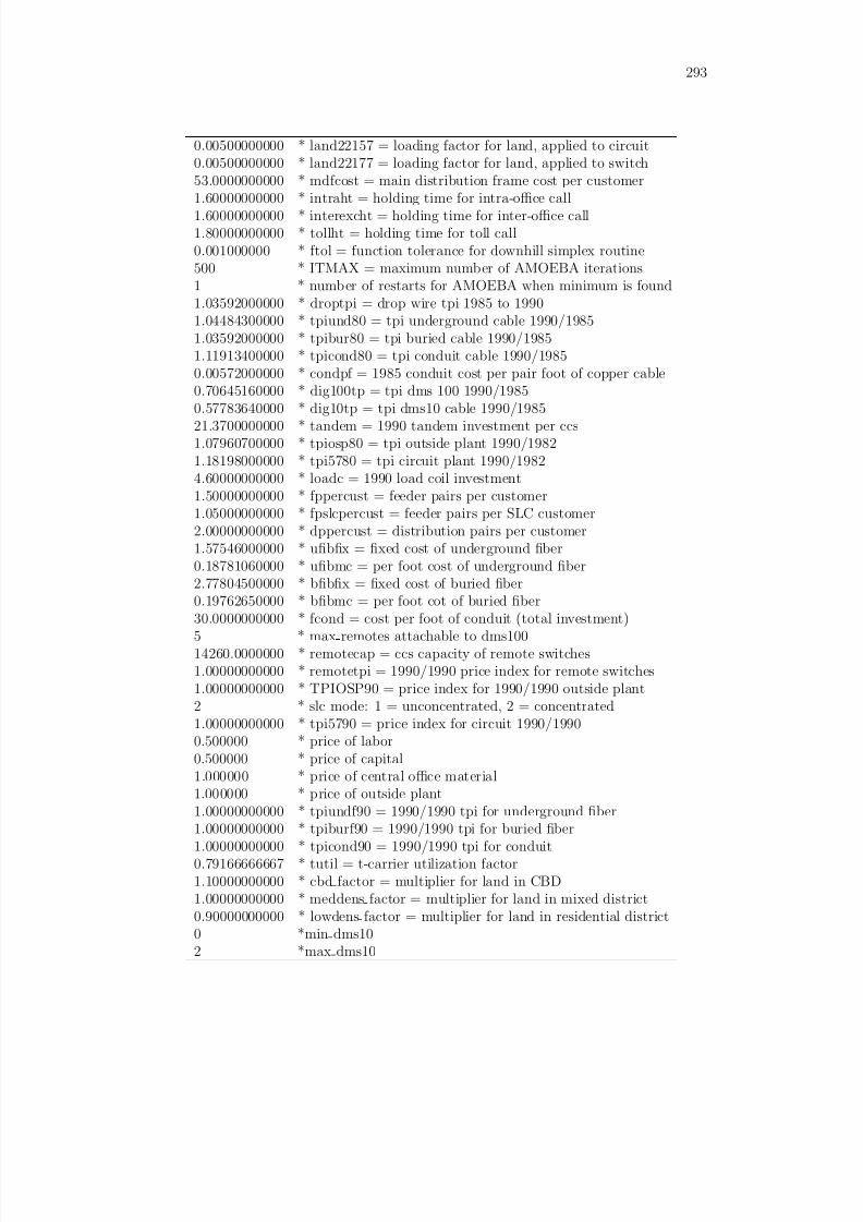
8/18/2019 Gasmi Cost Proxy Models
http://slidepdf.com/reader/full/gasmi-cost-proxy-models 293/318
293
0.00500000000 * land22157 = loading factor for land, applied to circuit0.00500000000 * land22177 = loading factor for land, applied to switch
53.0000000000 * mdfcost = main distribution frame cost per customer1.60000000000 * intraht = holding time for intra-office call1.60000000000 * interexcht = holding time for inter-office call1.80000000000 * tollht = holding time for toll call0.001000000 * ftol = function tolerance for downhill simplex routine500 * ITMAX = maximum number of AMOEBA iterations1 * number of restarts for AMOEBA when minimum is found1.03592000000 * droptpi = drop wire tpi 1985 to 19901.04484300000 * tpiund80 = tpi underground cable 1990/19851.03592000000 * tpibur80 = tpi buried cable 1990/1985
1.11913400000 * tpicond80 = tpi conduit cable 1990/19850.00572000000 * condpf = 1985 conduit cost per pair foot of copper cable0.70645160000 * dig100tp = tpi dms 100 1990/19850.57783640000 * dig10tp = tpi dms10 cable 1990/198521.3700000000 * tandem = 1990 tandem investment per ccs1.07960700000 * tpiosp80 = tpi outside plant 1990/19821.18198000000 * tpi5780 = tpi circuit plant 1990/19824.60000000000 * loadc = 1990 load coil investment1.50000000000 * fppercust = feeder pairs per customer1.05000000000 * fpslcpercust = feeder pairs per SLC customer2.00000000000 * dppercust = distribution pairs per customer1.57546000000 * ufibfix = fixed cost of underground fiber0.18781060000 * ufibmc = per foot cost of underground fiber2.77804500000 * bfibfix = fixed cost of buried fiber0.19762650000 * bfibmc = per foot cot of buried fiber30.0000000000 * fcond = cost per foot of conduit (total investment)5 * max remotes attachable to dms10014260.0000000 * remotecap = ccs capacity of remote switches1.00000000000 * remotetpi = 1990/1990 price index for remote switches1.00000000000 * TPIOSP90 = price index for 1990/1990 outside plant2 * slc mode: 1 = unconcentrated, 2 = concentrated
1.00000000000 * tpi5790 = price index for circuit 1990/19900.500000 * price of labor0.500000 * price of capital1.000000 * price of central office material1.000000 * price of outside plant1.00000000000 * tpiundf90 = 1990/1990 tpi for underground fiber1.00000000000 * tpiburf90 = 1990/1990 tpi for buried fiber1.00000000000 * tpicond90 = 1990/1990 tpi for conduit0.79166666667 * tutil = t-carrier utilization factor1.10000000000 * cbd factor = multiplier for land in CBD
1.00000000000 * meddens factor = multiplier for land in mixed district0.90000000000 * lowdens factor = multiplier for land in residential district0 *min dms102 *max dms10
8/18/2019 Gasmi Cost Proxy Models
http://slidepdf.com/reader/full/gasmi-cost-proxy-models 294/318
294 APPENDIX A
LECOM consists of three executable programs. The first program, “Cityinit.exe”
is used to create a set of serving areas based on the data in the populatn.dat file. Thisprogram needs to be executed only once unless the underlying populatn.dat file is modified.
As an output, cityinit writes a file called “rectangl.dat” which defines the upper right and
lower left boundaries of each serving area. If desired, this file can be created independently
of the cityinit program and used in subsequent calculations, as long as the data are
consistent with the populatn.dat file.
After the file rectangl.dat file has been created the file “dxinit.exe” is run in orderto compute copper to fiber crossover values. Finally, the main LECOM program, called
“Digital.exe” is run to compute loop investments while optimizing over the number and
location of switching machines as described in Chapter 2. The program Digital.exe should
always be run with command line options by calling “Digital -f -5.” These options tell
the program to write its outputs to a file called “digital.oda” which contains all of the
necessary outputs for subsequent data analysis. A representative output file is illustrated
in Table A.8.

8/18/2019 Gasmi Cost Proxy Models
http://slidepdf.com/reader/full/gasmi-cost-proxy-models 295/318
295
Table A.15
A Sample Digital.oda file9066863.79 total annual cost5 total number of switches0 number of dms10 switches4 number of remote switches2705435.20 annual cost of distribution plant2644365.83 annual cost of feeder plant2460468.72 annual cost of switching plant378012.14 annual cost of interoffice plant878581.9012 annual cost of main distribution frame
186 number of serving areas600 target lines per serving area581 actual lines per serving area18000 number of business lines54016 number of mixed density lines35968 number of residential lines8477 number of private lines0.4500 private line cost markup0.400000 private line toll percentage0.110000 business private line percentage0.075000 mixed density private line percentage0.068000 residential private line percentage29715.6407 intra-office message volume4800.8416 exchange inter-office message volume10779.9224 toll message volume95090.0501 intra-office ccs15362.6933 exchange inter-office ccs38807.7206 toll ccs0.260000 toll percentage1.500000 business ccs per line1.500000 mixed density ccs per line
1.500000 residential ccs per line2455.8235 averge loop length184.8236 length of slc-1.0000 price of labor0.5000 price of capital1.0000 price of central office materials1.0000 price of outside plant materials24.0000 24.0000 16.0000 16.0000 business district coordinates32.0000 32.0000 8.0000 8.0000 mixed density district coordinates40.0000 40.0000 city upper right coordinates
22.0745 20.0628 33.3916 26.7297 13.6222 37.9972 switch locations38.6403 3.7448 29.4541 37.5476 switch locations

8/18/2019 Gasmi Cost Proxy Models
http://slidepdf.com/reader/full/gasmi-cost-proxy-models 296/318
296 APPENDIX A
In order to automate the process of running large numbers of LECOM simulations in
order to generate data for the estimation of cost functions, several utility programs havebeen provided. The programs “setpop.exe” and “setinput.exe” allow the user to set the
parameters in the populatn.dat file and the output and price variables in the dvariabl.dat
file respectively. The syntax of each program can be determined by typing the name of
the program without arguments as in the following example.
C:\Lecom \setinput Error in command line parameters: 1
Correct syntax is SETINPUT [ccs res] [ccs med] [ccs bus] [PK][PL] [P COmat] [P OSmat]
Batch files have also been written to set appropriate inputs and run the relevant
LECOM programs in order to generate the data sets used in each chapter’s analysis. For
example, in order to duplicate the data used in chapters 6 and 7, the user should proceed
as follows. First make sure that the files pop Ch6.dat and dvar Ch6.dat are located in the
data directory. Then copy the batch program “run Ch6.bat” into the working directory,
C:\Lecom and run it by typing the DOS command “C:\Lecom\run ch6.bat”, or by using
the Windows “Run” command to execute this file. After the program has completed
operation, a set of output files will be located in the directory “C:\Lecom\output”. In
order to conveniently transfer these files into an Excel spreadsheet for further analysis,
the Excel Macro Extract(), which is contained in the workbook “data.xls”, may be used.
Once the data have been converted to a spreadsheet format they can by further pro-
cessed in a variety of ways and used in any standard econometrics package. Since all of the
analytical analysis which underlies chapters 5 through 9 in this volume was done using the
program Mathematica, we chose to read the data directly into a Mathematica notebook
and use the built-in regression routine to fit a trans-log cost function. The data and cost
functions computed for each of chapters 5 through 9 are contained in the notebook titled
“LECOM data.nb”.

8/18/2019 Gasmi Cost Proxy Models
http://slidepdf.com/reader/full/gasmi-cost-proxy-models 297/318
297
A.6 A Guide to The Mathematica Analysis
A separate Mathematica notebook is provided in the CD supplied in the book to document
the analysis used to obtain the results in each of Chapters 5 through 9. These notebooks
are provided “as is” with no attempt to fully document the commands contained in them.
Moreover, since the authors are not expert Mathematica programmers, the programming
logic contained in these notebooks represents by no means the most efficient method of
obtaining our desired results. Mathematica version 3.0 or higher is required in order to
make use of the notebooks.
Each notebook has been designed to run on a stand alone basis in order to perform the
necessary analytical computations to derive results used in the empirical sections of the
chapters. For each chapter, the interested reader should first evaluate the group of cells
labeled “Initialization” which defines all of the relevant functions and constants used in
the “Results” sections. It is recommended that only one chapter at a time be evaluated in
each Mathematica session, since the definitions and names of functions may differ slightly
from one chapter to another. Since the Mathematica Kernel “remembers” all definitions
until they are explicitly cleared, there is a possibility that unintended conflicts arise if two
or more chapters are evaluated in a single session.4 Each initialization section contains
the definitions of all of the functions used in our analysis: the cost function, demand
functions, disutility of effort function, and the regulator’s probability density function
over the type of firm. Based on these functions, all of the analytical results described in
chapter 4 and in the theoretical sections of chapters 5 through 9 can be given an explicit
representation, and in most cases solved. For the purpose of illustration, we consider here
the case of optimal (LT) regulation.
Recall from Section 6.2 the statement of the regulator’s problem, given in equations
(6.2) - (6.4). Solving (6.3) and (6.4) for the firm’s rent, and substituting into equation
(6.2) yields the reduced form regulatory problem given in equation (6.5) and repeated as
equation (A.7) below
8/18/2019 Gasmi Cost Proxy Models
http://slidepdf.com/reader/full/gasmi-cost-proxy-models 298/318
298 APPENDIX A
maxq(·),e(·)
β
β
V (q (β )) − (1 + λ) [C (β, e(β ), q (β )) + ψ(e(β ))]
+λF (β )
f (β )ψ(e(β ))
∂C (β, e(β ), q (β ))
∂β ∂C (β, e(β ), q (β ))
∂e
f (β )dβ.
(A.7)
In Mathematica notation, the integrand to equation (A.7) is given as follows:
LTIntegrand [q ,e ,b ] := (V[q]-(1+lambda)*(Cost[q,e,b]+psi[e])+ lambda*(F[b]/f[b])*psi’[e]*dcb[q,e,b]/dce[q,e,b]);
In the above expression, the functions dcb and dce represent the derivatives of cost with
respect to β and e respectively, and the other terms are exactly as defined in Chapter 6.
The functions q(.) and e(.) that solve the regulator’s problem (A.7) are therefore given by
the Mathematica functions LTQ[b ] and LTE[b ] which are solved for using the following
code.
LT[b ] := LT[b] = FindRoot[Evaluate[{D[LTIntegrand [q,e,b1],q]==0,
D[LTIntegrand [q,e,b1],e]==0}/.b1 → b],
{q,highq},{e,lowe}];
LTQ[b ] := q /. LT[b];
LTE[b ] := e /. LT[b];
The above expression directly solves the first-order conditions which are found by
differentiating social welfare with respect to q and e respectively for each value of b. The
firm’s rent is then determined by integrating equation (6.4) using the optimal values of q
and e for each value of b.
LTR[b ] := LTR[b] = NIntegrate[-psi’[LTE[b1]]*
dcb[LTQ[b1],LTE[b1],b1]/dce[LTQ[b1],LTE[b1],b1],
{b1,b,highb},PrecisionGoal → 3];

8/18/2019 Gasmi Cost Proxy Models
http://slidepdf.com/reader/full/gasmi-cost-proxy-models 299/318
299
Consumers’ welfare is solved using equation (6.1) and the fact that it is equal to social
welfare minus the firm’s rent, which gives the following Mathematica expressions.
CW[q ,e ,b ,U ] := V[q] - (1+lambda)*(U+psi[e]+Cost[q,e,b])
LTCW[b ] := CW[LTQ[b],LTE[b],b,LTR[b]];
LTSW[b ] := LTCW[b] + LTR[b]
A.7 Contents of the CDRom
Included with this volume is a CD which contains programs and data which will allow
the reader to verify virtually all of the reported results. Readers are encouraged to
experiment with these files by choosing alternative input assumptions. The files on the
CD are organized in 4 directories as follows:
LECOM
DATA
PROGRAMS
RESULTS
MATHEMATICA
CHAPTER 5
CHAPTER 6
CHAPTER 7
CHAPTER 8
CHAPTER 9
LECOM DATA
INSTALL HCPM: A program to install the most recent available version of HCPM along

8/18/2019 Gasmi Cost Proxy Models
http://slidepdf.com/reader/full/gasmi-cost-proxy-models 300/318
300 APPENDIX A
with source code and documentation.
INSTALL MATHREADER: A free program from Wolfram Research Inc. which allows
one to read the Mathematica notebook.

8/18/2019 Gasmi Cost Proxy Models
http://slidepdf.com/reader/full/gasmi-cost-proxy-models 301/318
NOTES 301
Notes
1The fact that in the cost functions presented below, with and without interconnection
costs accounted for, most of the parameters are identical is only the result of our rounding
to the second decimal. However, in this chapter, and in all the other chapters of the book,
we have carried out the calculations with a much higher precision.
2Recall from the text that here we make the assumption that when the number of
subscribers served by a firm varies, those subscribers are kept uniformly distributed over
the LECOM density zones constituting a total area of approximately 57 square miles.
3Again, the reader should keep in mind that calculations have been carried out with a
much higher precision than presented here.
4The user needs only to quit the Mathematica Kernel between chapters in order to
eliminate any possibility of conflict.

8/18/2019 Gasmi Cost Proxy Models
http://slidepdf.com/reader/full/gasmi-cost-proxy-models 302/318
302 NOTES
8/18/2019 Gasmi Cost Proxy Models
http://slidepdf.com/reader/full/gasmi-cost-proxy-models 303/318
Appendix B
In this appendix we present some recent work on alternative proxy models.
B.1 The Hybrid Cost Proxy Model (HCPM)
In previous chapters we have demonstrated the application of a particular cost proxy
model, LECOM, as an empirical tool in the investigation of issues of interest in the field
of telecommunications policy. LECOM has been a natural tool to use for our purposes
because it does not rely on proprietary company data for its operation and because of its
novel ability to estimate a fully forward looking cost function that optimizes the location
of switching centers in the local exchange network. Following the divestiture of the local
operating companies from A.T.&T. in 1984 a number of other engineering process models
of telecommunications have been developed by both industry sources and by regulatory
bodies. These models have become increasingly sophisticated in their modeling techniques
and in many respects the current generation of cost models are capable of providing a
significantly more detailed and accurate representation of cost than LECOM. In this
section we will briefly review the development of cost proxy models other than LECOM
and will describe in some detail the Hybrid Cost Proxy Model (HCPM) which was selected
by the FCC in 1998 for use in computing universal service support in high cost areas served
by non-rural companies in the United States.1 In section A.3 we describe the application
of the HCPM outside of the United States.
The proxy models such as the HCPM have been developed primarily as tools for
explicit regulatory policy objectives, which include estimating the costs of providing uni-
303
8/18/2019 Gasmi Cost Proxy Models
http://slidepdf.com/reader/full/gasmi-cost-proxy-models 304/318
304 APPENDIX B
versal service support to high cost areas, providing cost based support for the setting of
prices for interconnection and for the purchase of unbundled network elements, and gen-erally in providing regulators with an independent estimate of the forward looking cost
of providing local telecommunications services. The analysis of certain issues in incen-
tive regulation in earlier chapters provides an interesting counterpoint to these intended
applications, for as this analysis has stressed the regulator’s knowledge of the cost func-
tion is never perfect. We have formalized the imperfect information of the regulator by
separating two crucial input parameters that are outside of the regulator’s control. In
our standard representation of cost as a function C (q , β , e) the variable β represents the
technology type of the firm, about which the regulator knows only the probability distri-
bution function. The variable e represents the level of effort of the firm to engage in cost
minimization, which is chosen by the firm in response to the form of incentive contract
offered by the regulator.
While the availability of cost proxy models offers an important new tool to regulators
in the design of pricing and entry rules, the theory of incentive regulation, which our
earlier chapters seek to empirically test, suggests that there are limitations in the power
of this tool. A proper application of cost proxy models by regulators should be made
with full knowledge of these limitations. At the same time, however, the ever increasing
accuracy of proxy models can, and we believe should, be used to obtain new theoretical
insights of interest to telecommunications policy makers. It is our hope that the analysis
of this chapter, and more broadly of this book, can serve as a contribution to both the
theory of regulation and the application of regulatory theory to the actual market.
The HCPM consists of several independent modules - computer programs that read
relevant input data, perform the calculations relevant to a portion of the local network,
and print output reports for use in succeeding modules. The version of HCPM adopted by
the FCC in its universal service proceeding consists of three such modules: a clustering
algorithm which groups customer locations into neighborhood serving areas, a cluster
interface module which computes the area and line density of each cluster and assigns
8/18/2019 Gasmi Cost Proxy Models
http://slidepdf.com/reader/full/gasmi-cost-proxy-models 305/318
305
individual locations to cells in a grid structure, and a loop design module that uses
network design algorithms to connect the grid cells in each serving area to a centralserving area interface and subsequently connect each serving area interface to the central
office switch. The HCPM also includes a module that can be used to compute the cost
of switching and interoffice transport. The loop design and interoffice modules report as
outputs both total investment in network facilities and an estimate of annual expenses
associated with those facilities.
Since the primary intended use of forward-looking cost proxy models in the UnitedStates has been to estimate the cost of providing universal service support, most of the
development effort for such models in that country has been in the design of distribution
and feeder portions of the local exchange network. In this section we will review several
modeling approaches to this portion of the local network in some detail in addition to
describing the HCPM approach. In many countries other than the United States, cost
proxy models have been developed with the intention of providing estimates of the cost of
interconnection among networks. Accordingly the switching and interoffice portions of the
network have received more attention in these models, notably in the German intercity
cost model prepared for the German Regulatory Authority for Telecommunications and
Posts.2 The Japanese Ministry of Posts and Telecommunications (MPT) has also spon-
sored a Long Run Incremental Cost model of the local and intercity telecommunications
networks in Japan.3
One of the first engineering process models developed by Mitchell (1990) for the Rand
Corporation under contract with GTE of California and Pacific Bell Telephone Company.
This model was a significant departure from a series of earlier econometric studies which
sought to estimate the degree of scale economies in the local telephone industry following
the divestiture of AT&T. The Rand model developed simple representations of the major
components of the local network: loop, switching and interoffice links, and attempted to
calibrate these functions using data supplied by the client companies. The next significant
advance in proxy cost modeling was the development of LECOM, which we have described
8/18/2019 Gasmi Cost Proxy Models
http://slidepdf.com/reader/full/gasmi-cost-proxy-models 306/318
306 APPENDIX B
in detail in Chapter 2 of this study. LECOM differed significantly from the Rand model
by including specific computer algorithms and network optimization routines in the designof the network. Nevertheless, by current standards, both the Rand model and LECOM
are relatively crude in certain aspects of their modeling methods.
Recall from Chapter 2 the approach that LECOM takes to defining local serving
areas.4 A LECOM city consists of three regions of varying population density: a central
business district, a mixed commercial and residential district, and a residential or rural
district. Serving areas in LECOM always have a uniform population distribution withinthem and they are always rectangular in shape. Moreover, while the size of the serving
area, measured as the number of access lines, is specified as a user input, the shape of
the area is by default determined by an algorithm that seeks to subdivide each of the city
areas into an appropriate number of neighborhoods.
Other cost proxy models have adopted a similar approach to defining distribution
areas. For example, the Benchmark Cost Model (BCM), sponsored by an industry con-
sortium consisting of U.S. West, Sprint, NYNEX and MCI used Census block groups
(CBGs) as distribution serving areas, with the justification that CBGs on average have a
household count that is reasonably comparable to local serving area line counts, and more
importantly that CBGs represent a uniform nationwide statistical representation of popu-
lation by a disinterested government body. Since the original purpose of the BCM was to
estimate the relative costs of serving different regions of the country for purposes of pro-
viding universal service support for high cost areas, this latter advantage was justifiably
seen as an important modeling principle. A competing industry sponsored model known
as the Hatfield Model (HM) used the same modeling approach as the BCM although it
differed significantly in its choice of recommended input assumptions.5
Later versions of the BCM adopted a somewhat different modeling principle of a rival
industry sponsored model - the Cost Proxy Model sponsored by Pacific Bell and devel-
oped by an independent consulting firm. The resulting Benchmark Cost Proxy Model
(BCPM) followed a grid based approach which measured population in areas defined by

8/18/2019 Gasmi Cost Proxy Models
http://slidepdf.com/reader/full/gasmi-cost-proxy-models 307/318
307
one degree of longitude and one degree of latitude.6 Serving areas were constructed in
the BCPM either by forming collections of grid cells until an appropriate line count wasreached, or in heavily populated regions by subdividing grid cells. In rural regions, CBGs
typically include a large land mass in order to maintain a roughly constant population
count throughout the country. Since the BCM and HM assumed that population was uni-
formly distributed throughout the entire CBG, the grid based approach offered significant
modeling advantages in highly rural areas. Ultimately, however, a uniform distribution
within the serving area was assumed for computational tractability.
In response to the grid based approach of the BCPM, the HM sponsors introduced
a clustering algorithm in a later version of that model, which was renamed the HAI
model. A clustering approach uses individual customer locations rather than grid cells as
primary data points. A statistical algorithm is then used to identify natural groupings of
customers which can be served by a common interface point. The HAI clustering approach
and the significant customer location data preparation which was required to implement
it were ultimately chosen as the most accurate of the modeling approaches by the FCC
in its universal service proceeding. The particular clustering method used by the HAI
model, and more importantly the loop design algorithms, that remained largely intact
from earlier versions of BCM and HM, were not, however, used in the FCC approach.
Instead the approach of the HCPM in both of these areas was adopted based on evidence
that indicated that the latter approach was the most accurate available approach for
modeling both urban and rural areas.7
In the HCPM a clustering algorithm reads in the customer location input data, which
consists of the latitude and longitude of each residential and business location and the
number of access lines demanded at that location. If location data at this level of detail
is not available, the model is also capable of processing data at the Census block level
consisting a the location of an interior point of the block and an estimate of the number
of residential and business lines demanded by users within the block. In the latter case,
the model processes the block level data by creating a set of surrogate point locations

8/18/2019 Gasmi Cost Proxy Models
http://slidepdf.com/reader/full/gasmi-cost-proxy-models 308/318
308 APPENDIX B
randomly distributed in a square area the size of the original block.
An advantage of the clustering approach over earlier approaches is the ability of the
model to explicitly maintain a maximum copper distance constraint. Satisfactory quality
for both voice grade and digital services requires that copper loop plant must be restricted
to a maximum distance, where the distance depends on the quality of service offered. 8
In LECOM the distribution loop length is allowed to vary according to the endogenously
determined size of serving areas, but appropriate adjustments are made in the thickness
(gauge) of the copper cables that are used. In the clustering approach, distances arecontrolled, and the model is able to make use of higher gauge (and therefore less expensive)
cable.
Once the clustering process is complete the customer locations are assigned to a set of
grid cells that overlay each cluster. The grid cells resemble the grids used by the BCPM
except that the cells are an order of magnitude smaller in size - 360 feet on a side instead
of approximately 3000 feet – and the population of each cell is determined endogenously
by the model from the more detailed customer location data. A loop design module is
then called upon to build both distribution and feeder plant to each grid cell. The smaller
size of grid cells allows both distribution and feeder plant to be built to essentially the
exact customer locations in the case of distribution plant, and to the exact locations of
serving area interface (SAI) points in the case of feeder plant.
Both distribution and feeder portions of the local network are designed based on min-
imum cost spanning tree algorithms, which seek to determine the minimum cost configu-
ration of network links that connect customers to the SAI and SAIs to the central office
switch respectively. Earlier cost proxy model, including LECOM, BCPM and HAI used
different variations of a “pine tree” routing algorithm in which locations were connected
to a central point (SAI or switch) using a pre-determined set of routes along vertical and
horizontal axes, with no attempt to minimize either the distance of cost of the resulting
network.9
8/18/2019 Gasmi Cost Proxy Models
http://slidepdf.com/reader/full/gasmi-cost-proxy-models 309/318
309
While the loop design portions of the HCPM represent a significant advance over ear-
lier modeling approaches, the HCPM and proxy models generally have been criticized forfailing to take account of geographical barriers, such as bodies of water or extremely moun-
tainous terrain, which real operating telephone companies are forced to recognize when
they build loop plant.10 It is likely that future modeling efforts will seek to incorporate
local cost conditions in an increasingly sophisticated manner.
In terms of modeling switching and interoffice investments, there have been relatively
minor advances in the current generation of cost proxy models over the approaches takenby Mitchell and in LECOM. All of the approaches define a simple switching cost function
of the form
C = C 0 + a1AL + a2T + a3CA + a4M N
where
C 0 is getting started costAL is the number of access linesT is the number of trunksCA is the number of call attemptsMN is the number of minutes
and a1, a2, a3, and a4 are constants.
The difficulty in obtaining an accurate forward looking representation of this cost has
traditionally been in obtaining appropriate data to calibrate it. Neither switch vendors
nor switch buyers have been willing to publicly reveal the details of actual contracts, since
the market for switching capacity is thin, and both sides have incentives to withhold the
relevant information from competitors.
Interoffice investments have been modeled with increasing accuracy, much like invest-
ments in loop plant. As described in Chapter 2, LECOM designs a full mesh network
for interoffice communications, where the amount of traffic carried between individual
switches is assumed to be inversely proportional to the distance between them. While
early versions of the BCM did not attempt to model interoffice costs in any manner, choos-

8/18/2019 Gasmi Cost Proxy Models
http://slidepdf.com/reader/full/gasmi-cost-proxy-models 310/318
310 APPENDIX B
ing instead to represent interoffice investment as a fixed percentage of loop plus switching
investment, more recent versions of the BCPM and HAI models have incorporated algo-rithms which compute the SONET ring technologies which are increasingly used to link
both host remote configurations and host to tandem configurations. An international
version of the HCPM also computes the cost of SONET rings. The WIK model, which is
intended to apply to the entire German intercity network consists of a hybrid of full mesh
and SONET ring connections, based on a detailed traffic demand model for projected
traffic flows between switches.
B.2 International Applications of HCPM
At this writing, three countries outside the United States are in varying stages of adopting
some form of HCPM for use as a regulatory tool, with a likelihood of more adoptions as
the need for such a tool grows. In this section, we briefly describe the implementation
process in two of these countries, Argentina and Portugal. The third country, Peru, is
still in the very early stages and is not yet in a position suitable for written description.
Argentina and Portugal have approached the model selection process quite differently.
In Argentina, a research team under the Universidad Argentina de la Empresa (UADE)
began the initial work of developing data sources and proposing changes to model logic
suitable for the Argentian situation. This group was able to develop a funding resource
in collaboration with the World Bank by working with local telephone operators.11
The Portuguese modeling team, by contrast, has always been fully contained within the
independent quasi-governmental authority Instituto das Comunicaes de Portugal (ICP).
The Portuguese team used ICP resources to purchase and develop independent data
sources and modify the program for use in Portugal.12
Below we describe highlights of both nations’ experiences in the use of the model.

8/18/2019 Gasmi Cost Proxy Models
http://slidepdf.com/reader/full/gasmi-cost-proxy-models 311/318
311
Argentina
The UADE team began its process of adapting the model to the Argentinian reality by
first approaching local telephone operators to seek their support for developing the tool,
with an eye toward eventually turning it over to the Comisin Nacional de Comunicaciones
(CNC) for use in arbitrating interconnection disputes and for calculating universal service
subsidies.
UADE devoted the first portion of its effort to identifying two representative areas
for analysis. In the Argentinian model of liberalization, the country was divided into
two “LATA-like” regions in order to create two distinct franchises (which are ultimately
intended to be open to completely free entry). These franchises were sold at auction to
Telefnica de Argentina, a subsidiary of Telefnica de Espaa, and to Telecom Argentina, a
subsidiary of France Telecom. A city from each franchise area was chosen for the initial
study. In the case of Telefnica, the city chosen was Crdoba; Mendoza was the city from
Telecom’s area.
The UADE team gathered data from Argentina’s Instituto Nacional de Estadistica y
Censos (INDEC) at the manzana, or city block, level for Crdoba. The INDEC data include
information on the number of residences, number of business locations, and number of
employees at those locations (business data are only available at the radio level, which is
analogous to a Census block group in the U.S., and these are distributed uniformly across
manzanas).13
Manzanas are assigned to wirecenters according to their proximity to each central
office. At the time of the writing of this book, precise data on wirecenter boundaries are
not available in Argentina. Residential line counts are assumed to equal either the number
of residences or the number of residences “adjusted” by weighting according to the total
residential line count for each wirecenter. Business line counts are assigned by dividing
total business line count for the wire center evenly over all business locations within the
calculated wirecenter. Letting RLCM i and RM i be, respectively, the residential line count
8/18/2019 Gasmi Cost Proxy Models
http://slidepdf.com/reader/full/gasmi-cost-proxy-models 312/318
312 APPENDIX B
assigned to manzana i and the number of residences in that manzana, RLCWC j be the
residential line count for the wirecenter j, we have
RLCM i = RM i
j
RM jRLCWC j
Similarly, for business line counts in each manzana we have
BLCM i = BM i j
BM jBLCWC j
where RLCM i and BLCM i represent, respectively, residential locations and business line
count in manzana i and BLCWC j represents business line count for the wirecenter j.
HCPM has also been designed to accept detailed geological and topographical data,
such as maximum and minimum grade of elevation, soil type, depth to bedrock, and water
table. Unfortunately, such data do not exist in Argentina as yet so “average” values were
used.
One purpose of the UADE exercise has been to determine the effect of less-than-
optimal customer location data on cost estimates. To that end, Benitez et al. (2000)
essentially performed an experiment in which results from manzana-based data were com-
pared with data based on geocoded customer locations derived from an address database
maintained by Telefnica. A dataset with even less precision than the manzana data was
also created by aggregating manzana data. The study found that cost differentials be-
tween the most and least aggregated cases were only 3% to 5% for an urban area (Crdoba)
presumed to be typical of Argentina. This result is important for developing countries in
view of the high cost of collecting data in those countries.
Another thrust of UADE research is to estimate the cost of incumbents’ universal
service obligation. At this writing, the research team is gathering data for other locations
in Argentina in order to develop such estimates, but preliminary results have been pre-
8/18/2019 Gasmi Cost Proxy Models
http://slidepdf.com/reader/full/gasmi-cost-proxy-models 313/318
313
sented in several academic conferences. Using the Crdoba dataset, Benitez et al. (1999)
first calculated cost estimates for serving these urban wirecenters at the existing level of penetration. Other exercises included testing the sensitivity of the latter result to changes
in the cost of copper cable and the cost of capital. Finally, these authors calculated the
incremental cost associated with moving from current penetration levels to 100% service
penetration.
At this writing, Argentina’s Secretara de Defensa de la Competencia y del Consumi-
dor (Secretariat for the Protection of Competition and Consumers, the Argentian FederalTrade Commission) of the Economics Ministry, has announced that it plans to use the
HCPM for official universal service cost estimates and for refereeing interconnection dis-
putes. A committee consisting of representatives of industry operators, the government,
academia, and international experts will be convened to supervise data collection and
mandate changes to the structure of the model.
Portugal
The ICP has decided to follow a somewhat independent course within the European Union
in its approach to handling universal service and interconnection issues. The ICP is in
full agreement with EU policy, which mandates that long-run incremental cost be used
as the basis for decisions on these issues and that interconnection rates be set at the
local, single tandem and double tandem level. While the EU has employed consultantsto develop its own forward-looking costing methodology, ICP has been concerned that
the modeling approach used may not be sufficiently rich or detailed enough to accurately
reflect the reality of Portuguese topography and geography. There are also concerns
that the EU’s consultants, Europe Economics, following the example set by Oftel in the
United Kingdom, is developing a model that merely reflects a stylization of the existing
network and does not incorporate the economic notion of long-run cost (which would, for
example, include optimization of at least some network components based on prices and
usage profiles).
8/18/2019 Gasmi Cost Proxy Models
http://slidepdf.com/reader/full/gasmi-cost-proxy-models 314/318
314 APPENDIX B
The ICP modeling team has, at this writing, been successful in developing a cus-
tomer location database in an innovative way. No database exists for Portugal thatincludes georeferenced customer locations with an indication of demand at each point,
and population data collected by the Instituto Nacional de Estatsticas reports only at
the level of the freguesia, an administrative unit roughly equivalent to a U.S. township.
The Portuguese Instituto Geogrfico do Exrcito, or Army Geographic Institute (IGE), has
developed digitized maps showing the location and shape of every building, road, and
geographical feature in the country. These data are manipulated to work with HCPM as
follows.
Each shape record is assigned to a freguesia based on the coordinates of its centroid
using MapInfo software. Once all shapes within a freguesia are “identified,” the number
of business and residential lines in that freguesia are assigned to each location proportion-
ally to the area of the shape at that location. Residential line counts from the freguesia
are derived in one of two ways, either by using INE data on number of residences within
the freguesia, or by allocating total wirecenter line counts to the freguesia based on an
allocation rule. When the computer program developed at ICP has assigned a line count
to each shape, it then assigns each shape to a wire center by using either a minimum
distance criterion (the shape is attached to the nearest wire center) or by accepting in-
formation provided by the user on wirecenter boundaries. Finally, at the option of the
user, total lines within each wirecenter can be “trued-up” to reflect line counts for the
wirecenter.
Partial data on soil type, depth to bedrock, and water table are available for portions
of Portugal, and these data have also been applied to the model. The ICP team also
collected altimetry data to use in calculation of “slope,” or grade angle. The altimetry
data exist at a resolution of approximately 100 meters latticed throughout the country. A
computer program developed at ICP calculates the slope at each point by measuring the
change in altitude between the point and each of its neighbors, recording the maximum
value. Each value is converted into a grade angle using the appropriate trigonometric
8/18/2019 Gasmi Cost Proxy Models
http://slidepdf.com/reader/full/gasmi-cost-proxy-models 315/318
315
identity. A database is thus created for the entire country. MapInfo assigns each slope
value to a freguesia, and maximum and minimum values for that freguesia are calculated.
At this writing, ICP is engaged in calculating interconnection costs using the HCPM
interoffice module as well as calculating universal service costs using another innovative
methodology. In the U.S., universal service cost estimates are obtained by estimating
company statewide average costs using HCPM. If the overall company statewide average
cost exceeds a benchmark, the difference between the statewide average cost and the
benchmark is equal to the amount of subsidy for that company in that state. ICP proposesto calculate universal service costs in a manner more consistent with the understanding
of economists. Let B be a benchmark cost calculation. Let Ri(x) be a geographic radius
about wirecenter i such that the average cost of providing service to all customers within
Ri(x) is less than x. Let C (R) be the average cost of providing network service to all
customers within radius R of the wirecenter, and C (R) be the average incremental cost
of providing service to customers located outside of R.
Note that C (R) is a “metafunction,” or composite, of the HCPM cluster, cluster inter-
face, and feeder/distribution algorithms. That is, as R changes, the number of customer
locations to be included in the wirecenter “map” varies, and clustering must be redone to
establish the locations of serving area interfaces. The universal service subsidy USS for
wirecenter i is defined as
U SS i = maxB
{C (Ri(B)) − B, 0)}
The value is calculated using the classical bisection technique. The approach permits
universal service subsidy calculations to be made for each individual wire center and
reflects the incremental cost of only those lines requiring subsidy.
8/18/2019 Gasmi Cost Proxy Models
http://slidepdf.com/reader/full/gasmi-cost-proxy-models 316/318
316 NOTES
Notes
1The model platform selected in October 1998 consisted of the HCPM, an internally
developed model of the feeder and distribution network, along with a model of the switch-
ing and interoffice transport network developed by HAI Consulting in cooperation with
A.T.&T. and MCI. Input prices to calibrate the model were approved by the FCC in
October 1999, and support payments were begun under the new mechanism in 2000. The
model was approved for use only for large companies with more than 100,000 access lines.Smaller rural companies continue to be supported under an existing program based on
embedded costs.
2“An Analytical Cost Model for the National Core Network” prepared by Wissenschaftliches
Institut fr Kommunikationsdienste (WIK) Gmbtt. See also “An Analytical Cost Model for
the Local Network.” These reports are available on the RegTP web site at http://www.regtp.de.
3Our review of cost modeling approaches in not intended to be comprehensive. In par-
ticular, we do not review at all the so-called “top down” modeling approaches that have
been used by some regulatory bodies and consulting firms. A top down model uses aggre-
gate accounting data from incumbent telecommunications providers, with modifications
to attempt to insure that a forward looking cost estimate is obtained. Such modifica-
tions might, for example, exclude accounting costs associated with maintenance of analog
switching equipment. In contrast, a “bottom up” modeling approach seeks to model in
detail the individual components of the network. There has been a lively debate among
model proponents about the proper modeling technique to use for each intended appli-
cation. Clearly top down models are prone to including costs that are not truly forward
looking, whereas bottom up models are prone to missing certain hard to measure but
legitimate costs that firms would encounter on a forward looking basis.
4See especially Figure 2.2.
5The Hatfield Model was sponsored jointly by A.T.&T. and MCI after MCI defected
8/18/2019 Gasmi Cost Proxy Models
http://slidepdf.com/reader/full/gasmi-cost-proxy-models 317/318
NOTES 317
from the original BCM coalition. An earlier version of the Hatfield Model had been
proposed which did not use the existing boundaries of wirecenters, as all of the morerecent proxy models other than LECOM have chosen to do.
6At the equator a resulting grid cell is approximately 3000 feet square, though the
exact dimensions of cells depend on the distance from the equator. In most cases a grid
cell is substantially smaller than a CBG.
7The clustering algorithm used by HAI was rejected primarily because it was done
in a pre-processing stage of the model, which raised concerns about the openness and
accessibility of the data used. The HCPM loop design approach was chosen on the
basis of some statistical analysis by FCC staff demonstrating that the HAI approach
systematically underestimated the cost of providing service in very low density areas and
systematically overestimated the cost of providing service in high density areas. See FCC
platform order: Federal-State Joint Board on Universal Service, Fifth Report and Order,
CC Docket Nos. 96-45, 97-160, 13 FCC Rcd 21323 (1998).
8In the universal service adaptation of HCPM, a copper distance limit of 18,000 feet was
assumed as a default based on evidence that this amount of copper plant was compatible
with traditional voice grade service and an acceptable quality of digital service via modem.
Alternative service qualities, such as the provision of ADSL services using copper plant
would require significantly shorter copper distance.
9A minimum distance spanning tree algorithm minimizes the distance of the overall
network. Since the costs of a telecommunications network depend both on distance and
the number of access lines carried on each link in the network (which affects cable and
electronics costs), the HCPM algorithms take account of both distance and line related
costs.
10The HCPM incorporates a feature, first introduced by the BCM model, in which
terrain factors are identified with the Census block in which each customer resides,

8/18/2019 Gasmi Cost Proxy Models
http://slidepdf.com/reader/full/gasmi-cost-proxy-models 318/318