Gas Turbine Dynamic Dynamometry:

A New Energy Engineering Laboratory Module

Zhiyuan Yang1 (yangz@msoe.edu),

Hope L. Weiss2 (weiss@msoe.edu),

Matthew J. Traum3 (traum@msoe.edu)

Mechanical Engineering Department

Milwaukee School of Engineering

Abstract

To integrate energy topics into STEM curricula, an archive of “Energy Engineering Laboratory

Modules” (EELMs) is being developed by collaborating faculty and students at the Milwaukee

School of Engineering (MSOE). EELMs facilitate spiral insertion of energy engineering

experiments into college and high school STEM courses. By making innovative use of

inexpensive equipment, EELMs facilitate near-ubiquitous accessibility to energy curricula, even

for instructors with limited resources.

Gas turbines are paramount to modern energy production and transportation, and this critical

technology will continue its prominence as we pursue a renewable energy future. Exposure to

gas turbines through hands-on experiments could provide meaningful content for a range of

STEM courses. However, prohibitively expensive commercially available educational test stands

preclude gas turbine experiments from all but specialized engineering programs. Moreover, even

if gas turbine hardware is available, specialized dynamometer and data acquisition equipment are

needed to evaluate performance. Alternatively, virtual laboratories can offer rich simulated

experiences to promote learning, but they lack the stimulating tactile and tangible learning

experiences applied experiments provide.

We describe a method to accurately measure and predict the mechanical power output of a gas

turbine using the rational inertia of the turbine’s spinning components and friction in its bearings

as the load. The turbine’s time response to Dirac load inputs and its no-load responses to

compressed air input over a range of pressures are measured. This technique, called dynamic

dynamometry, requires only an inexpensive optical tachometer, a digital video recorder, and free

image capture software for data acquisition. Turbine power-versus-angular-velocity curves are

produced, which can be used for design, additional analysis, and teaching. An additional benefit

of this technique is that turbine rotational inertia is determined independently of knowing the

rotor’s geometry. So, the experiment can be completed without dismantling the turbine; or, if

desired, the measured rotational inertia can be independently verified by disassembling the

turbine to measure internal component geometry and mass.

In addition to obvious applications for anchoring classroom discussions in physics, mechanical

dynamics, fluid mechanics, and thermodynamics; this exercise offers unexpected teaching

1 Undergraduate Research Assistant

2 Assistant Professor

3 Assistant Professor, Corresponding Author

opportunities for courses including Numerical Methods, Experimental Methods, and Statistics.

Coarse data acquisition frequency necessitates conditioning the raw power-versus-angular-

velocity data to distinguish meaningful, accurate performance curves. Moreover, outliers can be

identified and eliminated via statistical techniques.

Introduction

Increasing energy-focused education is important to meet the growing demand for sustainability-

conscious technical professionals. Gas turbines are paramount to modern energy production and

transportation, and this critical technology will continue its prominence as we pursue a

renewable energy future.1 Thus, within STEM curricula, a need exists to provide practical,

hands-on training in gas turbine systems. In parallel, however, a pragmatic need remains to

balance energy-focused training with classical engineering and science fundamentals while

keeping institutional costs manageable. New energy course content and the laboratory

apparatuses used to deliver it must be carefully evaluated and integrated so as not to overburden

STEM programs or curricula.

Three approaches predominate the instruction of gas turbine systems in current engineering

curricula. First, gas turbine system theory can simply be taught in a lecture course without an

accompanying laboratory,2 which deprives students of hands-on experience. Second, the “virtual

laboratory” approach allows students to run simulated experiments on computers programmed

with gas turbine system models.3 At its best, this approach can provide audio-visually rich

reproductions of actual laboratory environments intended to mimic the physical reality of live

laboratory testing. Nonetheless, the models and virtual experiments are prescribed and students

still miss the pragmatic experience of applied, hands-on experimentation. Third, an experimental

gas turbine laboratory apparatus, either expressly built using an available turbine or purchased

through an educational manufacturer,4 can showcase actual experimental operation of these

systems. However, this approach is prohibitively expensive to most STEM programs that lack

dedicated gas turbine research divisions.

To integrate hands-on energy topics, particularly gas turbines, into STEM curricula, we propose

an alternative to creating virtual laboratories with no real hardware or investing in capitally-

intensive lab equipment. An archive of “Energy Engineering Laboratory Modules” (EELMs) is

being developed by collaborating faculty and students at MSOE, accumulated, and disseminated

to facilitate spiral insertion of energy engineering concepts into college and high school courses

across STEM curricula. EELMs are economical, hands-on, “turn-key” activities that can be

incorporated into any STEM curricula to introduce energy studies. For example, a series of

building energy audit exercises was recently created and described that harvests existing

buildings as living laboratories suitable for quantitative evaluation using an inexpensive audit

tool kit.5 Additionally, a small, inexpensive inverted downdraft wood gasifier for processing pine

chips into syngas was designed from a metal vacuum-flask-style thermos bottle. It was

constructed for less than $50 to teach students about biomass-to-energy processes.6

To create EELM hardware for gas turbine experimentation, we propose constructing the disk

turbine shown in Figure 1 using freely available instructions obtained on-line from the

Instructables Web site.7 This design uses platters harvested from obsolete computer hard drives,

which are often freely available at K-12 schools and colleges that periodically retire old

computers. Hard drive platters can also be cheaply obtained from computer hardware reuse sites

such as Craig’s List.

Disk turbines (also called boundary layer turbines or

Tesla turbines) differ from conventional aero-derived

turbines. Instead of gas impinging on aerodynamic

blade surfaces to produce lift and spin the shaft, disk

turbines rely on viscous shear between the working fluid

and flat disks to provide motive torque. As a result, disk

turbines typically operate at much higher rotational rates

with lower torque than their aero-derived counterparts,

and they typically operate at a lower energy conversion

efficiency.8 Nonetheless, since complex aerodynamic

blades need not be fabricated, disk turbines are

extremely easy and inexpensive to create, making them

ideal as centerpieces for a gas turbine EELM.

Experimental evaluation of engines and turbo-

machinery typically requires a dynamometer to measure

power curves – power output as a function of rotational

rate for a series of loads. Due to the high-rotation-rate

and low torque output by disk turbines, no

commercially-available dynamometers are suitable.

Moreover, significant characterization is required to

correctly design appropriate custom dynamometers,

which are also expensive to build.9 To avoid these costs and complications, we use a technique

called dynamic dynamometry, which uses the rotational inertia of the turbine spindle and the

friction in the bearings as the load. No separate dynamometer is needed to extract power curves.

This technique has already been used successfully by researchers to characterize tiny disk

turbines10

and disk turbines for space applications.11

We adapt it here for educational purposes.

Critical to our technique is determination of turbine rotational inertia. While rotational inertia can

be measured or estimated through multiple different techniques already reported in the literature,

we feel the dynamic dynamometer approach is superior in the context of educational labs. By

contrast, in the Energy Method,12

a light string attached to a weight of known mass is wound

around the turbine shaft. The mas is released, and it falls until it hits the ground. The spindle is

then allowed to spin down to rest. The turbine’s rotational inertia is determined from an energy

balance on the attached falling mass assuming friction in the bearings is constant with respect to

rotational velocity. We showed through experimental measurement that this constant-bearing-

friction assumption is invalid, suggesting that dynamic dynamometry can provide more accurate

rotational inertia measurements than the Energy Method. In the Geometry Method, a theoretical

formula is used to determine rotational inertia of a single rigid component of regular geometry.13

,

14 The drawbacks of this technique include need to break apart the turbine to measure its internal

geometry and inability to correctly evaluate turbines with irregular or complex geometry. By

Figure 1: Students will build and test

small disk turbines fabricated using

discarded computer hard drive platters

following Instructables guidelines.

This image was used under a Creative

Commons convention; original at:

http://www.instructables.com/file/FV0

S7YD5AQEP27YAST

comparison, the advantage of dynamic dynamometry is accurate assessment of turbine rotational

inertia with no knowledge of the turbine’s internal structure.

We explain in this paper how dynamic dynamometry techniques can be taught in the context of

four unique mechanical engineering classes: Dynamics, Numerical Methods, Thermodynamics,

and Experimental Methods. Along the way, we weave together all the steps of the technique

including measuring the turbine’s rotational inertia, extracting power curves, and eliminating

outliers from the data set. We suggest that these different experimental project components be

conducted in several unique courses across a STEM program’s curriculum. The benefits of

showing different aspects of the same experimental project across multiple courses have already

been illuminated in the literature.15

Experimental Demonstrations, Results, and Analysis

All experiments we describe use an inexpensive optical tachometer to enable continuous

measurement of the turbine shaft rotation rate, and a video recording device (we used the free

video capture feature on an iPhone). The video-recorded tachometer readout provides time

histories of the turbine shaft angular velocity during experimental events, which is the

fundamental data stream analyzed to extract turbine performance metrics.

To reduce data to useful form, free frame-by-frame

video viewing software was utilized (we chose VLC

Media Player16

). The approximate data sampling rate

was determined by placing a stopwatch in the video

recorder’s field of view and counting the number of

frames shot over some characteristic duration. Each

frame therefore shows the tachometer reading at a

sampling interval equal to the frame rate of the video

capture device used. An example of the entire set-up is

shown in Figure 2.

Note that for future classroom deployment of the

dynamic dynamometer EELMs, we plan to build and

use the Instructable turbine shown in Figure 1.

However, to develop and evaluate the underlying

techniques described here, we saved time and resources

by using a small pre-built disk turbine made available

by an industry partner. While this hardware switch will affect numerical quantities measured and

calculated (i.e., the pre-built turbine from industry has higher rotational inertia than the

Instructable turbine), the underlying techniques can be universally applied to any disk turbine.

Dynamics Course: Turbine Rotational Inertia Determination by Dirac Force Input

One technique for disk turbine spindle moment of inertia determination can be demonstrated in a

sophomore-level Dynamics course by applying particle kinematics and kinetics concepts

universally taught in this course. For the demonstration, the turbine is anchored just above head

Figure 2: Optical tachometer and stopwatch positioned in the same video

shot to enable video capture of turbine

spindle experimental rotational

velocity time histories for data

analysis.

height. One end of a long, light

string (we used sewing thread) is

secured to the turbine spindle, and

the other end is attached to a free

weight of known mass resting at

the elevation of the turbine. The

shaft is then rotated by hand,

allowing the string to wrap around

the shaft without doubling up on

itself. With video capture of

tachometer data enabled, the

weight is knocked to the floor,

spinning the turbine shaft with an

instantaneous input of force

provided by gravity acting on the

weight’s mass.

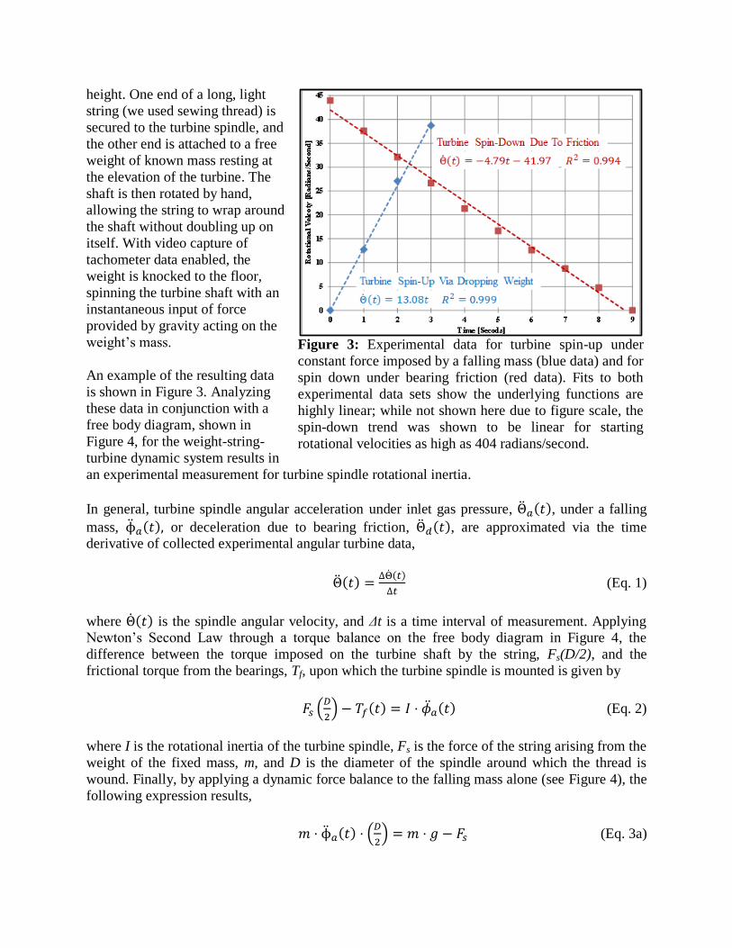
An example of the resulting data

is shown in Figure 3. Analyzing

these data in conjunction with a

free body diagram, shown in

Figure 4, for the weight-string-

turbine dynamic system results in

an experimental measurement for turbine spindle rotational inertia.

In general, turbine spindle angular acceleration under inlet gas pressure, ( ), under a falling

mass, ( ) or deceleration due to bearing friction, ( ), are approximated via the time derivative of collected experimental angular turbine data,

( ) ( )

(Eq. 1)

where ( ) is the spindle angular velocity, and Δt is a time interval of measurement. Applying Newton’s Second Law through a torque balance on the free body diagram in Figure 4, the

difference between the torque imposed on the turbine shaft by the string, Fs(D/2), and the

frictional torque from the bearings, Tf, upon which the turbine spindle is mounted is given by

(

) ( ) ( ) (Eq. 2)

where I is the rotational inertia of the turbine spindle, Fs is the force of the string arising from the

weight of the fixed mass, m, and D is the diameter of the spindle around which the thread is

wound. Finally, by applying a dynamic force balance to the falling mass alone (see Figure 4), the

following expression results,

( ) (

) (Eq. 3a)

Figure 3: Experimental data for turbine spin-up under

constant force imposed by a falling mass (blue data) and for

spin down under bearing friction (red data). Fits to both

experimental data sets show the underlying functions are

highly linear; while not shown here due to figure scale, the

spin-down trend was shown to be linear for starting

rotational velocities as high as 404 radians/second.

where g is the local gravitational acceleration. This expression can be solved for Fs:

( ) (

) (Eq. 3b)

To obtain an experimental function for Tf, the friction torque from the bearings, the unloaded

turbine was spun up to its maximum operational rotational velocity using compressed air. When

the turbine reached a steady state rate of rotation, the input gas was instantaneously shut off, and

the rotational velocity of the turbine with respect to time was logged while the turbine spun down

under friction primarily imposed by the bearings. A torque balance on the decelerating turbine

spindle alone yields

( ) ( ) (Eq. 4)

where ( ) is determined from Equation 1. Substituting Eq. 4 into Eq. 2 and rearranging gives

(

)

( ) ( ) (Eq. 5)

and plugging the Fs expression of Equation 3b into Equation 5 results in an expression to

determine I values exclusively from experimentally-measured inputs,

[ ( )

](

)

( ) ( ) (Eq. 6)

Now, to determine the value for I, the numerical values of the

functions ( ) and ( ) were found at each time step: t1, t2, … tn. These values were plugged into Equation 6, which

produced N-1 values for I where N is the total number of data

points. The reported value for I is the average of all the

discrete I values for each time step while the uncertainty in I

is approximated as twice the standard deviation of all the

data.

Numerical Methods Course: Turbine Rotational Inertia

Determination by Torsion Spring

The turbine spindle moment of inertia, I , can also be

determined through an alternative experiment that uses an

oscillating torsional spring instead of a falling mass. This

technique, which uses numerical integration of rotational

velocity data to obtain rotational position, can be taught in a

junior-level Numerical Methods course to showcase a

practical application of numerical integration.

A torsional spring is connected to the disk turbine apparatus

Figure 4: Free body diagram for

weight-string-turbine system

showing acceleration directions,

forces, and torques acting on

components.

Turbine Disk

Turbine

Shaft

Falling

Mass

String

a

D

Fs

mg

Tf

Fs

allowing for oscillatory dynamic analysis of this system. With the data-logging system running,

the torsional spring is twisted to give an initial displacement to the system. Using Newton’s

Second Law, the governing differential equation is

(Eq. 9)

where β is the coefficient of viscous friction; κ is the known torsional spring constant; and , ,

and are turbine angular acceleration, velocity, and displacement respectively. The major

assumption for this experimental setup is that the frictional torque is viscous, . The

rotational velocity, in radians/second, measured using the tachometer, is numerically integrated to obtain the angular position, Θ in radians. Another option for the experimental setup

would be to use an absolute encoder, if available, to measure the angular position of the shaft

directly.

Using the angular position of the turbine shaft determined via either method described, students

can determine the un-damped natural frequency, ωn, and damping ratio, ζ, using the logarithmic

decrement method. The natural frequency and damping ratio are related to the moment of inertia,

I, the coefficient of viscous friction, β, and the torsional spring constant, κ, by

√ ⁄ (Eq. 10)

and

√ (Eq. 11)

The moment of inertia can then be found from the two equations with two unknowns (I,β).

If both methods for determining turbine spindle rotational inertia are presented to a single class,

the students can then compare the results from each method while discussing the merits and

drawbacks of each. Furthermore, since the Instructable disk turbine can be disassembled, each

spindle part can be weighed, and their dimensions measured. The resulting rotational inertia can

then be built up analytically by superposition as an additional point of comparison and

discussion. Students typically learn this technique in Dynamics but are rarely able to practically

test it in that course.

Thermodynamics Course: Turbine Power Curve

Turbine power output as a function of rotational velocity, the so-called turbine power curve, can

be extracted experimentally by dynamic dynamometry. If the pressure at which compressed air is

input to the turbine is modulated by a regulator, a family of power curves can be produced,

showing the turbine’s power output for a range of input pressures. Finally, if a volume flow rate

meter is integrated into the gas line, the ratio of turbine power output to the total energy input

gives turbine energy conversion efficiency. All of these aspects of turbine performance can be

taught in a junior- or senior-level Thermodynamics course.

To illustrate turbine power curve measurement, we ran the turbine shown in Figure 2 using a

range of input pressures: 90 psi, 80 psi, 70 psi, 60 psi, 50 psi, and 40 psi. Pressure upstream of

the turbine was held constant using a regulator. While higher and lower pressures were available,

we deemed 100 psi too high for safe disk turbine operation. We also found that the turbine would

not spin up on its own for input pressures less than 30 psi. Increments of 10 psi were used for

convenience because the resulting power curves are easily distinguished from one another and

the regulator pressure gauge used read out in 10 psi increments.

To perform necessary data

acquisition in a lecture or lab

course, the pressure regulator

is set to a desired preset

value. Video capture of

tachometer data is initiated

with the turbine at rest. The

turbine gas inlet is

instantaneously opened, and

the turbine is allowed to spin

up until its rotational velocity

reaches steady state (we

describe later how ‘steady

state’ is formally defined). To

get a ‘feel’ for steady-state

operation, during the turbine

spin-up process, the bearings

will audibly whir. The pitch

will continue to grow higher

as the turbine accelerates.

When the pitch of the

turbine’s audible whir stops

increasing, this is a

qualitative indication that

steady state rotational velocity has been reached. To ensure steady state was, in fact, achieved in

all our data sets, each experiment was allowed to proceed for 60 seconds beyond the time

indicated by a steady pitch in the turbine’s audible whir. The resulting experimental data is

shown in Figure 5 for 90 psi input pressure.

The following derivation leads to a turbine power curve expression. The turbine’s moment of

inertia, I, is already known from the above-described analysis in the Dynamics and Numerical

Methods courses. The turbine’s power output, Pout, is

( ) ( )

( ) (Eq. 9)

since the output shaft torque, Tout, is

Figure 5: Rotational velocity versus time for a disk turbine spun

up from rest at constant input pressure. The experimental data

(blue diamonds) follow an asymptotic exponential, Equation 11,

(red curve) where the system time constant, τ, must be selected

to provide the best data/model fit. Data collected after time = 4τ

are redundant and can be eliminated from the analysis.

0

50

100

150

200

250

300

350

400

450

500

550

600

0 20 40 60 80 100 120 140 160 180

An

gu

lar

Velo

cit

y [

Ra

dia

ns/

Seco

nd

]

Time [Seconds]4τ = 115 s

Useful Data Redundant Data

Model Curve

Experimental Data

( )

(Eq. 10)

To find an equation for Pout, a functional form is needed for ( ). This function can be

determined by inspection. An example raw ( ) data set is given in Figure 5, and it is apparent

from the non-zero initial slope that the functional for ( ) is a first order response (an

asymptotic exponential) of the form

( ) (

) (Eq. 11)

where is the maximum turbine rotational velocity achieved at steady-state, and τ is a time

constant characteristic of the system.

To fit Equation 11 to the experimental data and obtain a useful functional for ( ), the time constant, τ, is treated as a variable parameter that is adjusted to achieve the best

equation/experiment match. The fitting technique we used was minimization of the Standard

Error of the Estimate (SEE). SEE is the sum of all the absolute differences between model and

experiment at each discrete time step. Figure 5 shows the exceptional experiment/model fit

between real data and Equation 11 when τ is selected to minimize SEE.

Identifying the correct value for τ enables further useful data reduction by approximating the

time at which turbine steady state rotation rate was achieved. All data collected after this time

can be discarded as redundant. We used 4τ as the number of time constants required for the

system to reach steady state. This decision is justified via the following analysis. At time =

0, ( ) . For a functional form of ( ) (

), at time = 4τ, ( )

(

) . At time → ∞, ( ) . Therefore, the percent error of

( ) at time = 4τ relative to at time → ∞ is given by the following calculation:

( )

( )

(Eq. 12)

In other words, the percent error of ( ) relative to is less than 2%, which we deem to

be an acceptable engineering approximation in characterizing this system. If additional error

reduction is desired, data can be retained for a duration of nτ where n is an arbitrary number

selected based on the level of precision needed for calculations.

Given the experimentally determined functional form of ( ) in Equation 11, the turbine output power, Pout, can be expressed by carrying out the derivative implied in Equation 9

( )

( )

[ ( )]

( )

( )

(Eq. 13)

which reduces through the following algebraic manipulations to a second-order polynomial

equation:

( ) [

] (Eq. 14a)

( ) [ (

)] (Eq. 14b)

( ) [ ( )] (Eq. 14c)

Therefore, the power output final formula is obtained,

[ ( ) ( )

] (Eq. 14d)

For a particular compressed air input pressure, experimental values for τ and are

determined using techniques described above. The representaive emperical turbine power curve

of Equation 14d can be plotted for the series of rotataional velocities measured at each discrete

time step during turbine spin-up. Figure 6 shows a family of example power curves for the disk

turbine of Figure 2 over the following range of input pressures: 90 psi, 80 psi, 70 psi, 60 psi, 50

psi, and 40 psi.

Another imporant

question relevant to

Thermodynamics is

how well the

emperical power

curve model of

Equation 14d

matches the

turbine’s actual

performance. The

most direct

approach would be

to attatch a

dynamometer to

the turbine to

experimentally

extract a measured

power curve.

However, as stated

above, disk

turbines require

expensive

customized

dynamometers whose creation is beyond the scope of a STEM program without a specilized

turbine research division. As an alternative, therefore, it is reasonable to extract power data

directly from dynamic dynamomtry by using an approximate differential form of Equation 9.

Figure 6: A family of power curves representing Equation 14d extracted

through empirical dynamic dynamometry measurements using an unloaded

disk turbine operating over a range of input pressures.

0.0

0.5

1.0

1.5

2.0

2.5

3.0

3.5

4.0

4.5

0 50 100 150 200 250 300 350 400 450 500 550

Po

wer

[W

att

s]

Rotational Velocity [Radians/Second]

90 PSI

80 PSI

70 PSI

60 PSI

50 PSI

40 PSI

( )

( ) (Eq. 15)

Here, the differential rotational velocity measured during turbine spin-up at each time step

substitues for the pure derivative allowing the turbine power output at each rotational velocity to

be quantified. An example of the resulting comparision between the emperical power curve

model of Equation 11 and the discrete turbine power versus rotational velocity represented by

Eqauation 15 is shown in Figure 7 for the representative case of 90 psi compressed gas inlet

pressure.

Experimental Methods Course: Data Outlier Elimination

Once the empirical power curve model and discrete turbine power versus rotational velocity are

available, the match between model and experimental data and the data’s quality can be

evaluated. In engineering curricula, the analytical tools to make this type of assessment are

typcially taught in Experimental Methods courses, but the analysis could also be framed in the

context of a mathematics course in Statisitics.

Model/Experiment agreement can be visually qualitatively evalauted by plotting both sets

together, as is shown in Figure 7 for the representative case of 90 psi turbine inlet pressure. The

experimetnal data follow the same second order polynomial curve as the model with the ( ) for both maximum power and for when output power is extinguished, which occur respectively

at rotational velocities similar to those predicted by the model. To gain further insight, the data

can be fitted with a quadratic regression (we added this trend using embedded tools in Microsoft

Excel – see Figure 7), which illustrates the second-order curve best fitting the data. Owing to the

coarse data acquisition frequency and the need for manual data input, the experiment is prone to

instances of random error. This susceptibility provides an educational opportunity to demonstrate

how to identify possible outliers and apply statistical techniques to decide whether they can be

legitimately eliminated from the data set.

For each data point, we calculated the absolute difference between output power determined

experimetnally and output power suggested by the best-fit polynomial for the data. These

differences were then averaged to obtain , and their standard deviation, , was calculated.

The farthest outlying point was then interrogated using Chauvenet's Criterion,17

| ( )|

(Eq. 16)

where Z is the number of standard deviations by which the suspect outlier differs from the

average. Then ( ) is evaluated using a normal error integral of a Gaussian distribution;

( ) is the probability that a legitimate measurement will differ from by a magnitude of

Z or more standard deviations. If it is found that

( ) (Eq. 17)

where N is the total number of measurements taken before an elapsed time of 4τ, then the suspect

outlying data point is thrown out.

The quadratic regression is then re-fitted to the remaining data, a new average and standard

deviation are calculated, and the the next farthest outlying point is evaluated via the process

above. Outlier elimination continues until all remaining data points satisfy Chauvenet’s

Criterion. Figure 7 shows the progression of quadratic regression curve fits to the experimental

data as outliers failing Chauvenet’s Criterion are eliminated. As outliers are eliminated,

agreement between the experimental curve fit and turbine output power predicted by Equation

14d continues to improve, further justifying this elimination process.

An important interpretive and educational question to ask is: how much does the outlier

elimination process actually move the fitted curve? In other words: how much do the outliers

impact the turbine’s predicted performance? Of paramount importance to turbine evaluation is

predicting and operating at peak power and identifying the rotational velocity that maximizes

this output power. For the disk turbine we characterized operating at 90 psi inlet pressure, the

predicted peak power output was about 4.53 Watts before removing outliers. After outlier

elimination, the predicted peak power fell to about 4.42 Watts, a 2.49% difference in power

output. This difference is probably not large enough to be concerning from a practical engineer’s

perspective, but it is large enough to show difference in magnitude and position of the fitted

curve before and after outlier elimination. Perhaps of greatest value in an Experimental Methods

course is that this random-error-prone experiment allows students to actually use Chauvenet’s

Criterion in a real application to eliminate outliers. Most of the time (at least in our anecdotal

laboratory teaching experience), students do not get to practice a formal technique to eliminate

outliers because lab experiments are usually well-tuned so as not to produce anomalies. Often,

Figure 7: Example theoretical versus experimental turbine power curves obtained from dynamic

dynamometry. (Left) With all raw data intact, the fitted polynomial over-predicts performance;

outlying data failing Chauvenet’s criterion are encircled in black. (Right) By removing outlying

data points, the resulting theoretical/experimental agreement is further improved.

0.0

0.5

1.0

1.5

2.0

2.5

3.0

3.5

4.0

4.5

5.0

5.5

0 100 200 300 400 500

Ou

tpu

t P

ow

er [

Wa

tts]

Angular Velocity [Radians/Second]

0.0

0.5

1.0

1.5

2.0

2.5

3.0

3.5

4.0

4.5

5.0

5.5

0 100 200 300 400 500

Ou

tpu

t P

ow

er [

Wa

tts]

Angular Velocity [Radians/Second]

Outliers

Power Curve –All Raw Data Intact Power Curve – Outliers Eliminated

Experimental Data Points

Theoretical Power Curve

Best Fit 2nd Order Polynomial Before Outlier Elimination

Best Fit 2nd Order Polynomial After Outlier Elimination

students want to throw out data points because they do not “look right” or they do not match the

theory. Applying Chauvenet’s Criterion to real data gives students a formal toolset to

quantitatively evaluate the validity of data points that look suspicious.

Conclusion

Within STEM curricula, a need exists to provide practical, hands-on training in gas turbine

systems while keeping institutional costs and additional program credit hours manageable.

Presented here is a method to accurately measure and predict the mechanical power output of a

small disk turbine running on compressed air that requires minimal, inexpensive, and easily

accessible equipment. The disk turbine itself is extremely easy and inexpensive to create making

it an ideal centerpiece for a gas turbine EELM. To avoid need to purchase or build a custom

dynamometer, we showcase a technique called dynamic dynamometry, which requires only an

inexpensive optical tachometer, a digital video recorder, and free image capture software for data

acquisition.

The dynamic dynamometry techniques can be taught through four unique mechanical

engineering classes: Dynamics, Numerical Methods, Thermodynamics, and Experimental

Methods. The disk turbine’s rotational inertia can be measured experimentally using knowledge

and skills typically taught in undergraduate courses in Dynamics and Numerical Methods. In the

context of a junior- or senior-level Thermodynamics course, we show how to derive the power

curve equation for a turbine, eliminate redundant data, and use the remaining data to correctly fit

a single empirical parameter to define power curves. Finally, we show how outliers among the

data can be identified and eliminated via statistical techniques that would be taught in a junior- or

senior-level Experimental Methods course.

Acknowledgements

We gratefully acknowledge EASENET, Inc. for project financial and material support as well as

the Wisconsin Space Grant Consortium 2012-2013 Higher Education Incentives Award Program

for financial support. This paper’s undergraduate lead author is a member of the Milwaukee

Undergraduate Researcher Incubator (MURI) at MSOE, an organization which fast-tracks

undergraduates into meaningful early research experiences.

Bibliography 1 L. S. Langston, “The Adaptable Gas Turbine,” American Scientist, Vol. 101, July-August 2013, pp. 264-267.

2 W. A. Woods, P. J. Bevan, D. I. Bevan, “Output and Efficiency of the Closed-Cycle Gas Turbine,” Proceedings of

the Institution of Mechanical Engineers, Part A: Journal of Power and Energy, Vol. 205, No. 1, February 1991, pp.

59-66. 3 K. Mathioudakis, N. Aretakis, P. Kotsiopoulos, E. A. Yfantis, “A virtual laboratory for education on gas turbine

principles and operation,” ASME paper GT2006-90357, Proceedings of the 2006 ASME Turbo Expo: Power for

Land, Sea, and Air, Barcelona, Spain, May 8-11, 2006. 4 Turbine Technologies, LTD., “MiniLab™ Gas Turbine Lab,” URL:

http://www.turbinetechnologies.com/EducationalLabProducts/TurbojetEngineLab.aspx, accessed 7/27/2013.

5 M. J. Traum, “Harvesting Built Environments for Accessible Energy Audit Training,” Proceedings of the 2nd

International Conference on the Constructed Environment, Chicago, IL, October 29-30, 2011. 6 M. J. Traum, J. A. Anderson, K. Pace, “An Inexpensive Inverted Downdraft Biomass Gasifier for Experimental

Energy-Thermal-Fluids Demonstrations,” Proceedings of the 120th American Society for Engineering Education

(ASEE) Conference and Exposition, Atlanta, GA, June 23-26, 2013. 7 Instructables Web Site, “Build a 15,000 rpm Tesla Turbine using hard drive platters,” URL:

http://www.instructables.com/id/Build-a-15,000-rpm-Tesla-Turbine-using-hard-drive-/, accessed 7/23/2013. 8 T. A. Emran, “Tesla Turbine Torque Modeling for Construction of a Dynamometer and Turbine,” M.S. Thesis,

University of North Texas, May 2011. 9 T. A. Emran, R. C. Alexander, C. T. Stallings, M. A. DeMay, M. J. Traum, “Method to Accurately Estimate Tesla

Turbine Stall Torque for Dynamometer or Generator Load Selection,” ASME Early Career Technical Journal, Vol.

10, pp. 158-164, 2010 [URL: http://districts.asme.org/DistrictF/ECTC/2010ECTC.htm]. 10

V. G. Krishnan, Z. Iqbal, M. M. Maharbiz, “A micro Tesla turbine for power generation from low pressure heads

and evaporation driven flows,” Proceedings of the 16th

International Solid-State Sensors, Actuators and

Microsystems Conference, June 5-9, 2011, Beijing, China, pp. 1851-1854. 11

Z. Yang, H. L. Weiss, M. J. Traum, “Dynamic Dynamometry to Characterize Disk Turbines for Space-Based

Power,” Proceedings of the 23rd Annual Wisconsin Space Conference, Milwaukee Wisconsin, August 15-16, 2013. 12

A. Mishra, Practical Physics for Engineers, Firewall Media, 2006. 13

Kruger Ventilation, “Starting Torque of Fan,” TBN019.1/2001, URL:

http://www.krugerfan.com/brochure/publications/Tbn019.pdf, accessed 9/8/2013. 14

B. Bolund, H. Bernhoff, M. Leijon. “Flywheel energy and power storage systems,” Renewable and Sustainable

Energy Reviews, Volume 11, Number 2, 2007, pp. 235-258. 15

M. J. Traum, V. Prantil, W. Farrow, H. Weis, “Enabling Mechanical Engineering Curriculum Interconnectivity

Through An Integrated Multicourse Model Rocketry Project,” Proceedings of the 120th American Society for

Engineering Education (ASEE) Conference and Exposition, Atlanta, GA, June 23-26, 2013. 16

VCL Media Player, URL: http://www.vlcapp.com/vlc-features/frame-by-frame-video-player/ , accessed

7/30/2013. 17

J. R. Taylor, An Introduction to Error Analysis The Study of Uncertainties in Physical Measurements, 2nd

Ed.,

University Science Books, Sausalito, CA, 1997.