Embed Size (px)
Citation preview

203
The Energy Journal, Vol. 32, No. 1, Copyright �2011 by the IAEE. All rights reserved.
* Corresponding author. Professor of Finance, Norwegian School of Economics and BusinessAdministration (NHH). E-mail: [email protected].
** Professor of Finance, Norwegian School of Economics and Business Administration (NHH).*** Business Analyst, Viz Risk Management.
Gas Storage Valuation:Price Modelling v. Optimization Methods
Petter Bjerksund*, Gunnar Stensland**, and Frank Vagstad***
In the literature, one approach is to analyse gas storage within a simpleone-factor price dynamics framework that is solved to optimality. We follow analternative approach, where the market is represented by a forward curve withdaily granularity, the price uncertainty is represented by six factors, and wherewe impose a simple and intuitive storage strategy.
Based on UK natural gas market price data, we obtain the gas storagevalue using our approach, and compare with results from a one-factor model aswell as with perfect foresight. We find that our approach captures much more ofthe true flexibility value than the one-factor model.
1. INTRODUCTION
In the literature, the analysis of natural gas storage has traditionally beenintegrated with the valuation of other activities of the company, for instance pro-duction, supply, and demand. However, the existence of a natural gas forward/futures market motivates the use of decision support models from finance. Thebasic idea is to consider gas storage as a separate asset, and use the market valueframework for valuation and utilization of this asset. The company can deal witheconomic risk by trading in the financial gas market, and cover possible physicalimbalances in the spot market.
Several of the methods in recent literature that are applied from financeare aimed at solving the gas storage problem to optimality. One example is LeastSquares Monte Carlo (LSMC) of Longstaff and Schwartz (2001), which is appliedto gas storage by for instance Boogert and de Jong (2008).
Longstaff and Schwartz (2001) use the LSMC to evaluate an Americanstock option to optimality, assuming the usual stock price dynamics. However,
204 / The Energy Journal
the natural gas market consists not only of a spot price but of a whole family offorward prices. Moreover, market data show: (i) clear seasonal price patterns; (ii)considerable price uncertainty; and (iii) more than a few factors are needed toexplain the price uncertainty.
In order to solve the gas storage to optimality and still retain computa-tional efficiency, the number of state variables has to be limited. This means thatthe actual problem has to be simplified substantially. Optimality is at best attainedwithin the simplified framework. So an important question is how much of the“true” gas storage flexibility value is assumed away by reducing the problem toone that can be solved to optimality.
We apply an alternative approach based on a detailed representation ofthe forward curve and its dynamics, combined with an intuitive and feasibledecision rule that follows from repeated maximization of the intrinsic value. Ateach decision point, the market is represented by an updated forward curve thatis consistent with the quoted market prices and that reflects relevant historicalinformation (typical time profiles). We apply Principal Component Analysis(PCA) to identify the (six) factors and determine their loads from actual forwardcurve movements. We use Monte Carlo simulations to model possible realisationsof the forward curve dynamics, where the decision that is locked in at each pointin time follows from maximizing the intrinsic value of the gas storage.
Our valuation model is tested on market data from the UK NationalBalancing Point (NBP) covering a two-year period. We compare the results fromour approach with the results from a one-factor optimization model as well aswith unfeasible perfect foresight (ex post optimization). The results indicate thatour approach, with a rich representation of the forward price dynamics combinedwith a simple and intuitive decision rule (repeated intrinsic value maximization),captures much more of the actual flexibility value than solving gas storage tooptimality within a one-factor model framework.
2. SPOT PRICE MODELS
Boogert and de Jong (2008) present a spot price model for valuation ofgas storage. They assume that the spot price dynamics are
dS(t)�j[l(t)–ln S(t)]dt�rdW(t) (1)
S(t)
where the mean-reversion rate and the instantaneous spot volatility are posi-j rtive constants. The long-term level is a time-varying function that can bel(t)used to fit the spot price process to the forward curve at the initial evaluationdate. This model is referred to as the log-normal mean-reverting Ornstein-Uhl-enbeck price process. Hodges (2004) and Chen and Forsyth (2006) consider asimilar price model.
Boogert and de Jong (2008) use (1) above to simulate the spot pricepaths. These paths, combined with the characteristics of the gas storage, are then

Gas Storage Valuation: Price Modelling v. Optimization Methods / 205
analyzed by LSMC. Chen and Forsyth (2006) combine a regime-switching pricemodel with the storage characteristics to set up an optimal control problem. Thesolution to this problem gives the storage value.
In our opinion, a one-factor framework is not appropriate for modellinga gas storage. We will give several reasons.
Firstly, the model above is a one-factor spot model. A one-factor modelfor gas and electricity is unrealistic. Koekebakker and Ollmar (2005) find that upto 10 factors are needed to explain the price movements in the Nord Pool elec-tricity market. Our data indicate that we need six factors to explain 90% of thevariation in the NBP gas market in UK.
The reason for choosing a one-factor framework is basically dictated bythe focus on the solution method. Boogert and de Jong (2008) find stable resultsfor a number of fewer than 5 000 price paths. Increasing the number of factorswill dramatically influence this result.
Suppose we extend the model above to a three-factor spot model. Withinthe LSMC approach, we then need to estimate a decision rule that is made con-ditional on the value of these three factors for every time step and for every stateof the reservoir. Li (2007) suggests the regression
[V ]t�1 1 2 3E �� �� exp(y )�� exp(y )�� exp(y )t 0 1 t 2 t 3 t� �Ft
1 2 3 1 2 3�� exp(2y )�� exp(2y )�� exp(2y )�� exp(y �y �y ) (2)4 t 5 t 6 t 7 t t t
where are the different factors. The choice might be good but it isiy ;i�1,2,3t
still arbitrary. There is an endless number of basis functions of the three factorsthat are not included above. In this paper we propose a six-factor forward pricemodel. This model is unsuitable for a LSMC solution procedure. The reason isthat the estimation of the decision rule will be unfeasible.
Secondly, the initial forward curve used to calculate the trend above playsan unrealistic role. In order to start with a model that is consistent with the currentmarket situation, the trend in the above spot price model is calibrated to theforward market prices that are quoted at the initial date. This creates sensitivityto the initial forward curve that is unrealistic. It will also create problems for apossible hedging strategy.
Thirdly, it is unclear how to back-test the model over a given period. Wemay run into problems if we want to compare the value calculated initially withthe value we obtain from running the storage following this decision rule. Inpractice we will never assign that much weight on the initial forward curve. Sincemarket prices do not follow a one-factor model we will observe a new trendfunction every day. Given that we stick with the old trend function, we takepositions on a certain market view. The result will depend on whether this marketview is profitable or not. The outcome will be very erratic.
And finally, a storage may be interpreted as a complex calendar spread.It is well known from Margrabe (1987) that the flexibility value of an option to
206 / The Energy Journal
exchange one asset for another is zero if the two asset prices are perfectly cor-related. One-factor models basically focus on more or less parallel shifts of theforward curve, which means that forward price returns for different points at thecurve are highly correlated. Such forward curve movements will have limitedimpact on the storage decision as well as the value of the storage flexibility.
3. VALUATION MODEL
In the following we describe our method for evaluating the storage. Weadopt the standard assumptions from contingent claims analysis of a completemarket with no frictions and no riskless arbitrage opportunities, see, e.g., Coxand Ross (1976), Harrison and Kreps (1979), and Harrison and Pliska (1981).
3.1 Forward Curve
We assume that the company faces a decision problem with daily gran-ularity. Consequently, the company should use information with the same gran-ularity. The key information in the gas storage problem is the forward curve,hence we need a forward curve with daily granularity.
It follows from economic decision theory that the current forward pricefor a given day may be interpreted as the certainty equivalent value of that day’sfuture spot price, given the current information. We argue that the forward curveshould to be consistent with updated market information (quoted forward contractprices) and relevant historical information (typical time profiles).
3.2 Forward Curve Dynamics
We assume that the risk adjusted dynamics of the forward curve can berepresented by a general multifactor model. See, for instance, Heath, Jarrow, andMorton (1992), Bjerksund, Rasmussen, and Stensland (2000), or Clewlow andStrickland (2000). For an overview of different forward curve methods, see Ge-man (2005).
The dynamics of the forward curve are represented by the followingequation
NdF(t,T)� r (t,T)dZ (t) (3)� i iF(t,T) i�1
where represents the forward price at time for delivery at time . TheF(t,T) t Tvolatility is represented by where . The increments of ther (t,T) i�1, . . . ,N Ni
Brownian motions are assumed independent.dZ (t)i
The dynamics just above translates into the future forward price being
t tN 1
2F(t,T)�F(0,T)exp r (u,T)dZ (u)� r (u,T)du . (4)� i i i� �2� � �i�10 0

Gas Storage Valuation: Price Modelling v. Optimization Methods / 207
Every day, we construct a forward curve with daily granularity. Next we find areturn function for each day as a function of time to delivery. Then we performprincipal component analysis (PCA) to find typical curve movements. The vol-atility functions follow from the loadings in the PCA.
We assume that the volatility functions are time homogeneous, i.e.,
r (t,T)�r (T�t);i�1, . . . ,N . (5)i i
Eq. (5) means that the loadings from the PCA depend only on time to delivery(maturity) and not on calendar time (season). The assumption brings our modelin line with the one-factor model from the existing literature that we use as ourbenchmark, where the volatility is not seasonal. However, the absence of season-ality in the factor loadings may be considered a strong assumption. This modelis not likely to detect possible seasonal volatility in the data. The assumptionmight be relaxed if we find ways of estimating PCA-components as a functionof calendar time as well as time to delivery.
To perform the simulations we apply the following discrete time repre-sentation of (4)
N 12F(t�Dt,T)�F(t,T)exp (r (T�t) Dt•e � r (T�t)Dt) . (6)� i i i� 2i�1
Equation (6) is used to simulate the forward curve at time conditional ont�Dtthe forward curve at time , where we draw independent standard normal dis-t Ntributed numbers , .e i�1, . . . ,Ni
3.3 Intrinsic Value
Based on a forward curve with daily granularity we find the optimaldeterministic strategy. This is done by solving the following dynamic programwhere both time and reservoir are discretizised
Dr t�V(i, j)�max (e V(ik�{�min(j,2);0;min(J�j,1)}
�1, j�k)�p(i)uk�c(i, j, k, p(i))) (7)where
V(i,j):value functioni: time index (day), i�{1,2, . . . ,I}, where iDt : time (years)j: reservoir index, j�{0,1,2, . . . ,J}, where uj: reservoir (million therms)k: storage decision variable, k�{–2,–1,0,1},
where –: deplete uk units of gas�: inject uk units of gas
p(i): daily price from the forward curvec(): cost functionr : interest rate per annum
208 / The Energy Journal
We model a storage technology where the magnitude of the maximum depletionrate is twice the (maximum) injection rate. We assume that at the horizon ,IDtthe storage is returned to its initial size . This is enforced by the terminaluj0
condition
�1000 million pounds ∀ j�j0V(I, j)��0 j�j0
The costs may be made dependent on time, reservoir, depletion/injection, as wellas the gas price.
Some authors (see, e.g., Eydeland and Wolyniec (2003)) refer to theintrinsic value as the optimal initial plan that might be locked in using the tradableproducts. The implicit assumption seems to be that the granularity of the decisionproblem corresponds to the product calendar of the market. Now, suppose a prob-lem with a one-year horizon and that only a one-year contract were traded in themarket. The intrinsic value of storage would then be zero, according to the abovedefinition. This is clearly meaningless. In most markets, there are traded forwardcontracts on a monthly delivery (swaps). The definition above would then dis-regard the possibility of following one strategy during weekdays and anotherstrategy during weekends, which would translate into an unrealistically low re-ported number for the intrinsic value.
In the following, we define the intrinsic value as the expected value ofstorage given the risk adjusted dynamics in Section (3.2) above, conditional onfollowing the best initial deterministic plan. The reason for our definition of theintrinsic value is as follows. A contract on a monthly delivery can be interpretedas a portfolio of contracts on daily deliveries. However, the fact that there is onequoted marked price for the monthly contract does not necessarily mean that eachdaily contract commands the same (forward) market price. Although daily con-tracts are not traded except for in the very short end of the curve, we know fromempirical data that there typically will be time-dependent price differences in thefuture, for instance between weekends and weekdays. Since we start out with aforward curve with a higher granularity (daily) than the product calendar in themarket, our intrinsic value will exceed the value of the traditional intrinsic plan.
3.4 Repeated Intrinsic Value Method
We start out with the initial forward curve and find today’s intrinsic plan.From this plan we lock in the storage decision regarding today. If the decision isto fill, the storage is increased and the cost of filling follows from the current spotprice. If the decision is to deplete, the storage reservoir is decreased and therevenue follows from the current spot price. If the decision is to stay put, thereis no cash flow and the reservoir is unaltered.
Next we simulate a realisation for tomorrow’s forward curve conditionalon today’s forward curve and the price dynamics given in Section (3.2). For this

Gas Storage Valuation: Price Modelling v. Optimization Methods / 209
new forward curve, tomorrow’s intrinsic plan is determined. This problem isupdated for the storage decision that is already locked in as well as the passageof time (one day closer to the terminal date). This plan is used to lock in thestorage decision regarding tomorrow. We continue this procedure until we reachthe terminal date of our problem.
This procedure gives us one possible realisation of daily cash flows fromthe storage over the relevant time horizon. We repeat the procedure above toobtain the desired number of possible cash flow realisations. The value of storageis given by the average net present value of the simulated daily cash flows.
3.5 Comparing with a One-factor Optimization Model
In this paper we claim that the focus on stochastic optimization methodsleads to an oversimplification of the price modelling that severely undervaluesthe value of storage. In order to compare results, we consider the one-factor modelin Boogert and de Jong (2008).
The starting point is the discrete-time version of (1), where the spot pricedynamics is calibrated to the initial forward curve by
2S(t) 1 rjt 2jt� �S(t�Dt)�F(0,t�Dt)exp e ln + (1�e )� � � � �F(0,t) 2 2j
2 21 r r2j(t Dt) 2jDt� � �� (1�e )� (1�e )e (8)2 2j 2j
where and are the spot prices at time and , andS(t) S(t�Dt) t t�Dt F(0,t)are the initial forward prices for delivery at time and , respec-F(0,t�Dt) t t�Dt
tively, is standard normal, and is the time step size. We use (8) to simulatee Dtpossible spot price path realisations. Each path is mapped into a discrete spotM
price state space (51 states). Based on the discrete spot price path realisations, weobtain a spot price transition matrix for each calendar day. Within this framework,the storage problem is solved to optimality by stochastic dynamic programming.
4. STORAGE VALUATION—AN EXAMPLE
4.1 Data
We use natural gas price data quoted at NBP from October 1st 2004–September 30th 2006. The prices are quoted by pence/therm. The traded contractsare spot, day ahead, balance of week, balance of month, as well as calendarmonths and seasons (summer and winter).
We use the Elviz Front Manager software to translate this price infor-mation into a forward curve with daily granularity that is consistent with themarket prices of the quoted contracts and that reflects typical seasonalities over

210 / The Energy Journal
the week and over the year. A detailed outline, which includes a solution method,is given in Benth, Koekebakker and Ollmar (2007).
The forward curve at NBP at October 1st 2004 is illustrated in Figure1. Observe that there are price variations within the week (lower prices duringweekends) and within the year (higher prices during the winter season).
Figure 1: Forward Curve on Oct 1st 2004
Principal components analysis (PCA) is a widely used method for sim-plifying complex data structures. The basic idea is to identify the most importantfactors (principal components) and use them to represent the market. For an in-troduction to PCA of forward curves, see for instance Blanco et al. (2002). Basedon the forward curve movements the first year, we apply PCA to estimate theloadings. The loadings of the first six components are given in Figure 2.
Figure 2: Loadings of the Six Most Important Factors

Gas Storage Valuation: Price Modelling v. Optimization Methods / 211
1. The eigenvalues associated with the 6 first components are 0.27; 0.17; 0.12; 0.05; 0.04; and0.02.
The first component can be recognized as a parallel shift of the forwardcurve, which typically will have a small impact on the gas storage value. Thesecond component seems to represent a tilting of the forward curve, but it is farfrom a linear tilt. The third component can be interpreted as a change in curvature.The other three components are more difficult to give intuitive explanations. How-ever, the combinations of these six factors give rise to a rich class of possibleforward curve movements.
The explanation power of the components is shown in Figure 3. Observethat the first factor (parallel shift) explains about 35% of the variation, whereas75% of the variation can be attributed to the three first factors. We want to explainabout 90% of the price variation, hence we settle for six factors.1
Figure 3: Cumulative Percentage Variance Contribution of PrincipalComponents
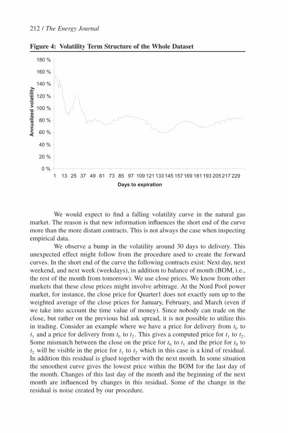
In Figure 4 we present the volatility term structure for the whole dataset.The graph using only six factors gives a similar picture.
212 / The Energy Journal
Figure 4: Volatility Term Structure of the Whole Dataset
We would expect to find a falling volatility curve in the natural gasmarket. The reason is that new information influences the short end of the curvemore than the more distant contracts. This is not always the case when inspectingempirical data.
We observe a bump in the volatility around 30 days to delivery. Thisunexpected effect might follow from the procedure used to create the forwardcurves. In the short end of the curve the following contracts exist: Next day, nextweekend, and next week (weekdays), in addition to balance of month (BOM, i.e.,the rest of the month from tomorrow). We use close prices. We know from othermarkets that these close prices might involve arbitrage. At the Nord Pool powermarket, for instance, the close price for Quarter1 does not exactly sum up to theweighted average of the close prices for January, February, and March (even ifwe take into account the time value of money). Since nobody can trade on theclose, but rather on the previous bid ask spread, it is not possible to utilize thisin trading. Consider an example where we have a price for delivery from tot0
and a price for delivery from to . This gives a computed price for to .t t t t t1 0 2 1 2
Some mismatch between the close on the price for to and the price for tot t t0 1 0
will be visible in the price for to which in this case is a kind of residual.t t t2 1 2
In addition this residual is glued together with the next month. In some situationthe smoothest curve gives the lowest price within the BOM for the last day ofthe month. Changes of this last day of the month and the beginning of the nextmonth are influenced by changes in this residual. Some of the change in theresidual is noise created by our procedure.

Gas Storage Valuation: Price Modelling v. Optimization Methods / 213
2. The mean and standard deviation over all simulations for the profit-and-loss from the physical(unhedged) storage is 190 and 78 million pounds, respectively. This gives a standard deviation of the
4.2 Storage Characteristics
The characteristics of the stylized storage are given in Table 1.
Table 1: Storage Characteristics
Initial storage 125 million therms
Terminal storage 125 million therms
Max storage 250 million therms
Injection 2.5 million therms per day
Depletion 2.5 or 5 million therms per day
Hence, an empty storage can be filled in 100 days, whereas a full storage can beemptied in 50 days. All costs are set to zero, and we disregard the positive interestrate. We consider a problem with a one-year horizon, and our objective is toobtain the value of the cash flow from operating the storage.
4.3 In-sample Analysis
We start with an in-sample valuation example, where we consider thevalue of operating the storage facility the first year (October 1st 2004 to Septem-ber 30th 2005), given the initial forward curve (Figure 1) and using the PCAfactor load estimates from the same period (Figure 2).
The traditional intrinsic value that can be locked in using the tradedmonthly products is 58 million pounds. The intrinsic value using daily resolutionof both the forward curve and the storage strategy is 77 million pounds.
The one-factor model in Equation (8) (5 000 simulations used to generatetransition matrices), optimizing the storage strategy, gives a value of 104 millionpounds. Here we have used the short term volatility of 149% per annum and amean-reverting rate of 0.05 per day, which translates into a rate of j�0.05 •
per year. The short term volatility is a proxy for the short term volatility in365the PCA-components, whereas the mean-reverting rate is equal to the rate usedby Boogert and de Jong (2008).
Given the initial forward curve and the estimated factor loadings, thesix-factor model with repeated intrinsic value maximization gives a storage valueof 187 million pounds (1 000 simulations). The standard deviation of this estimateis 1.1 million pounds. This means that the value of flexibility is considerablyhigher than reported by the other models. In order to obtain rather low standarddeviation in the estimate using only 1 000 simulations, we use the value of thefinancial hedging strategy as a control variate (see Section 5).2

214 / The Energy Journal
physical storage value estimate (1 000 simulations) of 2.5 million pounds. The mean and standarddeviation over all simulations for the profit-and-loss from the financial hedge is –3.4 and 83 millionpounds, respectively. This gives a standard deviation of the financial hedge value estimate (1 000simulations) of 2.6 million pounds. The correlation between the profit-and-loss from the physicalstorage and the financial hedge is –0.90.
As a comparison, we find that the optimal but unfeasible perfect foresightmethod gives a storage value 205 million pounds (1 000 simulations). The stan-dard deviation of this estimate is 2 million pounds. This result is obtained bysimulating all the forward prices paths to the horizon, finding the correspondingspot price path, and the ex post best strategy for each path.
Our results are summarized in Table 2.
Table 2: Calculated Storage Value2004 (million pounds)
Intrinsic—monthly granularity 58
Intrinsic—daily granularity 77
One-factor model 104
Dynamic intrinsic method 187
Perfect foresight 205
On this background we claim that the simple repeated intrinsic method is closeto the optimal value. We know that the perfect foresight value of 205 millionpounds is impossible to obtain.
4.4 Out-of-sample Analysis
Next we consider an out-of-sample analysis. In this example, we con-sider the value of operating the storage facility the second year (October 1st 2005to September 30th 2006), using the initial forward curve at October 1st 2005 andthe PCA factor load estimates from the first year (October 1st 2004 to September30th 2005).
Figure 5: Forward Curve Comparison
Gas Storage Valuation: Price Modelling v. Optimization Methods / 215
3. The mean and standard deviation over all simulations for the profit-and-loss from the physical(unhedged) storage is 233 and 98 million pounds, respectively. This gives a standard deviation of thephysical storage value estimate (1 000 simulations) of 3.1 million pounds. The mean and standarddeviation over all simulations for the profit-and-loss from the financial hedge is –4.6 and 105 millionpounds, respectively. This gives a standard deviation of the financial hedge value estimate (1 000simulations) of 3.3 million pounds. The correlation between the profit-and-loss from the physicalstorage and the financial hedge is –0.88.
In this case, the traditional intrinsic value that can be locked in using thetraded monthly products is 61 million pounds, whereas the intrinsic value of thestorage with daily resolution is 74 million pounds. These numbers are quite closeto the corresponding values of the first year reported in Table 2 above. To explainthis, observe that the storage may be interpreted as a complex calendar spread,and that forward curves at October 1st 2004 and October 1st 2005 basically havethe same shape (relative prices), c.f. Figure 5.
The one-factor model, where we use Equation (8) (5,000 simulations)to generate transition matrices, and assume the same short-term volatility andmean reverting rate as above, gives a value of 116 million pounds. The repeatedintrinsic method gives a value of 228 million pounds (1,000 simulations usingcontrol variate).3 The standard deviation of this estimate is 1.5 million pounds.As a comparision, we find that the optimal but infeasible perfect foresight modelgives 258 million pounds (1,000 simulations). The standard deviation of thisestimate is 3 million pounds.
Our findings are summarized in Table 3.
Table 3: Calculated Storage Value2005 (million pounds)
Intrinsic—monthly granularity 61
Intrinsic—daily granularity 74
One-factor model 116
Dynamic intrinsic method 228
Perfect foresight 258
4.5 Conclusions
The two examples show that our six-factor model, combined with re-peated intrinsic value maximization, creates a significantly higher value than theone-factor stochastic optimization model. Moreover, we find that there is a mar-ginal additional value from perfect foresight. Perfect foresight is of course un-feasible, and represents an upper bound to the true storage value. This indicatesthat our valuation approach captures most of the storage flexibility value, andsuggests that there is a limited potential for improvement of our approach in this

216 / The Energy Journal
example. Of course, there might be other storage characteristics not investigatedhere where one-factor models are more suited.
In our examples, we have abstracted from injection/depletion costs. Ifsuch costs are included, the investigated methods will give a lower storage value.However, it might be that the that dynamic intrinsic value method, which in asense utilizes more of the changes in curvature, will suffer a greater reduction invalue as compared to the one-factor model.
5. FINANCIAL HEDGE
A crucial point in option pricing theory is the concept of a replicatingportfolio. The rationale behind the Black-Scholes option pricing formula is theexistence of a dynamic self-financing trading strategy that gives exactly the samepay-off at the horizon. To rule out arbitrage, the option price must coincide withthe cost of creating the replicating portfolio. If we know how to replicate anoption, we also know how to hedge it, because the two strategies are opposites.However, the beauty of the theory often breaks down in practice. The most im-portant explanation is a mismatch of volatilities between the model and the mar-ket.
In the case of risk management of a gas storage, it may be instructive tothink in terms of a replicating portfolio. It will in typically consist of positions inall of the forward contracts. Since we are not even close to a formula for the gasstorage value, the load on every contract has to be simulated.
Consequently, we use an alternative approach to the hedging problem.In particular, we will exploit our dynamic intrinsic plan to define a financialforward trading strategy. The cash flow from this strategy will be highly nega-tively correlated with the cash flow generated from the gas storage. However, thestrategy will not capture the pure flexibility value that accrues to the owner ofthe physical facility. Hence we might call this a sub-replicating hedge portfolio.
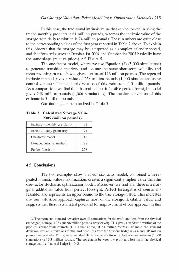
As an illustration, consider October 1st 2004. Suppose that we can tradedaily forward contracts at each point in time. The initial hedge portfolio wouldthen have an exposure as shown in Figure 6.
Gas Storage Valuation: Price Modelling v. Optimization Methods / 217
Figure 6: Exposure October 1st from Trades in the Forward Market
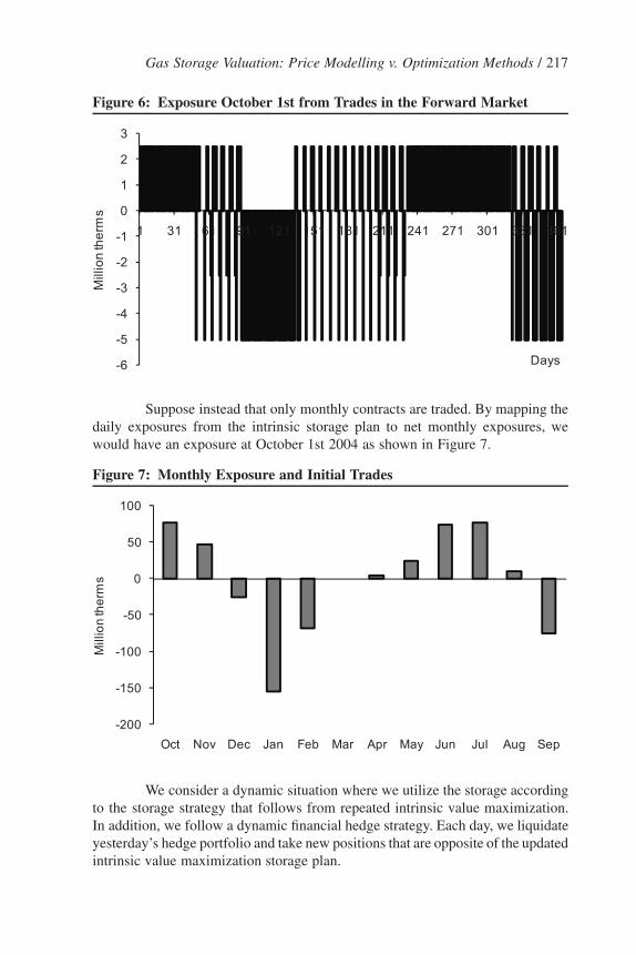
Suppose instead that only monthly contracts are traded. By mapping thedaily exposures from the intrinsic storage plan to net monthly exposures, wewould have an exposure at October 1st 2004 as shown in Figure 7.
Figure 7: Monthly Exposure and Initial Trades
We consider a dynamic situation where we utilize the storage accordingto the storage strategy that follows from repeated intrinsic value maximization.In addition, we follow a dynamic financial hedge strategy. Each day, we liquidateyesterday’s hedge portfolio and take new positions that are opposite of the updatedintrinsic value maximization storage plan.

218 / The Energy Journal
4. The value of launching the financial hedge strategy is zero. Consequently, the value of the(unhedged) storage must equal the value of a hedged storage. In the numerical analysis, the valuecorresponds to the average discounted pay-off. There is a strong negative correlation between thepay-off from the storage and the pay-off from the financial hedge. This means that we can improvethe accuracy of our value estimate by evaluating the hedged storage, i.e., to sum the value producedby the storage and the profit-and-loss from the financial hedging strategy for each simulation. See,e.g., Jackel (2002).
Recall that the hedge portfolio consists of forward contract positions.This means that the market value of entering each position (as well as the port-folio) is zero. Next day, new forward prices are quoted. The old hedge portfoliois then liquidated, yielding a positive or negative cash flow. Thereafter, the newhedge portfolio is composed using information from the updated intrinsic valuestorage plan. And so forth. It follows from above that the market value of launch-ing the dynamic hedge strategy is zero.
Observe that the hedge strategy can be implemented by any market par-ticipant. The gas storage ownership per se is no prerequisite for trading in thefinancial gas market. The storage can of course serve as collateral for the com-pany’s financial gas trading and speculation, but that is a different matter.
So why bother with such a strategy? The explanation is that the cashflows from the gas storage and the hedge portfolio are highly negatively corre-lated. One obvious practical application of our hedge strategy is to reduce therisk from owning and utilizing a gas storage. Another application is to improvethe accuracy of our gas storage value estimate by using the financial hedge strat-egy as a control variate.4
6. BACK-TEST
In this section, we investigate the performance of our dynamic intrinsicvalue maximization strategy on the spot prices that actually were realized in themarket. We assume the same storage characteristics as above and that terminalstorage equals the initial storage.
6.1 Year 1—Storage
We start at October 1st 2004 and consider the following year. Maximiz-ing the intrinsic value that day gives the strategy that is illustrated in Figure 8.

Gas Storage Valuation: Price Modelling v. Optimization Methods / 219
Figure 8: Storage from the Intrinsic Plan
The expected cumulative cash flow from sticking to this strategy is il-lustrated in the figure below, where we use the property that each day’s forwardprice can be interpreted as the expected future spot price that day (using theequivalent martingale measure).
Figure 9: Accumulated Cash Flow from the Intrinsic Plan
The cumulative expected cash flow starts out negative, which reflectsthat the strategy is to start injecting. The cumulative expected cash flow at thehorizon is the initial intrinsic value of 77 million pounds, c.f. Table 2.
We perform an intrinsic value model every day given updated infor-mation. In this example, we decide to fill the storage with maximum capacity

220 / The Energy Journal
equal 2.5 million therms this first day. The next day we have the forward curvegiven in Figure 10.
Figure 10: Forward Curve October 2nd 2004
We now optimize the intrinsic value for the remaining period given up-dated information. The current reservoir is 127.5 million therms. There are 364days to the horizon, and the terminal storage must equal 125 million terms.
Note that the strategy is almost unchanged. The best decision day twogiven that we follow the updated intrinsic plan is also to inject. We continue inthis way for every day. For the weekend we use the curve given on last Fridayto take the decision whether to inject or deplete.
We continue in this way until September 30th 2005. At this time thereservoir equals 125 million therms. The result for the dynamic intrinsic methodfrom October 1st 2004 until September 30th 2005 is given in the following fig-ures.
The evolution of the storage is given in Figure 11.

Gas Storage Valuation: Price Modelling v. Optimization Methods / 221
Figure 11: Actual Storage Size with the Dynamic Intrinsic Method Oct 1st2004 to Sept 30th 2005
The spot prices that were realized the first year is shown in Figure 12.
Figure 12: NBP Prices Oct 1st 2004 – Sept 30th 2005
The development of the accumulated cash flow from following the dy-namic intrinsic method is shown in Figure 13.

222 / The Energy Journal
Figure 13: Realized Accumulated Cash Flow from the Dynamic IntrinsicMethod Oct 1st 2004 – Sept 30th 2005
The result from the dynamic intrinsic value method is 48 million pounds.As a comparison, the result form perfect foresight (ex post optimization using therealized spot prices in Figure 12) is 60 million pounds.
6.2 Year 1—Hedged Storage
Above, we found that the realised cash flow from storage by imple-menting the repeated intrinsic value maximization from 1st October 2004 to 30thSeptember 2005 is 48 million pounds.
Now, suppose that the owner of the gas storage had launched a dynamicfinancial hedge strategy as described in the previous section. Assuming a marketwith daily forward contracts, the realised cash flow generated by the dynamicfinancial hedge portfolio was 185 million pounds. This large number can be ex-plained by the realized seasonal spreads are reduced as compared to the initialspreads. This adds up to a total cash flow from the hedged storage 233 millionpounds. The development of the cumulated cash is illustrated in Figure 14.

Gas Storage Valuation: Price Modelling v. Optimization Methods / 223
Figure 14: Accumulated Physical and Financial Value
It may be argued that daily forwards are unrealistic. In order to model amore realistic trading strategy, we assume that all exposure from the optimalintrinsic plan is mapped into net positions in the traded products. For simplicitywe assume that the next 10 days are tradable, and thereafter only the relevanttrading list from next month and to the horizon. The cash flow generated by thedynamic financial hedge is then reduced to 89 million pounds. This translatesinto a total cash flow from the hedged storage of 137 million pounds. The resultsof our back-test are summarized in Table 4.
Table 4: Back-test Results 2004 (million pounds)
Storage strategy Physical storage
Perfect foresight (unfeasible) 60
Dynamic intrinsic method 48
Hedge strategy Financial hedge Hedged storage
Trading calendar 89 137 (� 48 � 89)
Daily forwards 185 233 (� 48 � 185)
6.3 Year 2—Storage
Now we perform the same analysis for the year starting at October 1st2005 with a one-year horizon. The reservoir is the same as in the previous example125 million therms. The first day we obtain the following intrinsic value results.

224 / The Energy Journal
Figure 15: Accumulated Cash Flow from the Intrinsic Plan
The expected cumulative cash flow from sticking to the initial intrinsicplan next year is 74 million pounds. This is close the initial guess the year before.It is the seasonal spread in the forward curve that creates this value. It is thereforefair to say that this pattern is unchanged.
Next we perform a new intrinsic value model every day until September30th 2006. The reservoir is left at the same size as we started with, that is 125million terms. The result from this strategy is presented below. The evolution ofthe storage is given in Figure 16.
Figure 16: Actual Storage Size with the Dynamic Intrinsic Method Oct 1st2005 to September 30th 2006
The spot prices that were realized the second year are shown in Figure17.
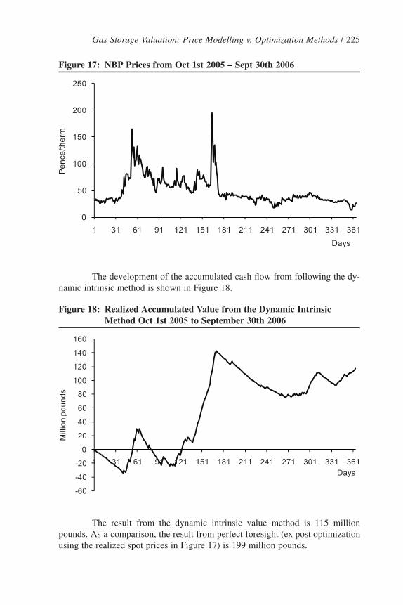
Gas Storage Valuation: Price Modelling v. Optimization Methods / 225
Figure 17: NBP Prices from Oct 1st 2005 – Sept 30th 2006
The development of the accumulated cash flow from following the dy-namic intrinsic method is shown in Figure 18.
Figure 18: Realized Accumulated Value from the Dynamic IntrinsicMethod Oct 1st 2005 to September 30th 2006
The result from the dynamic intrinsic value method is 115 millionpounds. As a comparison, the result from perfect foresight (ex post optimizationusing the realized spot prices in Figure 17) is 199 million pounds.

226 / The Energy Journal
6.4 Year 2—Hedged Storage
Assume a market with daily forward contracts. The dynamic hedgingstrategy in this case gives a trading profit of 325 million pounds. So the value ofthe hedged storage amounts to 440 million pounds.
If we only include the 10 first days of forward prices and the tradingcalendar which starts with the next full month, the result drops to 190 millionpounds. The results of our back-test are summarized in Table 5.
Table 5: Back-test Results 2005 (million pounds)
Storage strategy Physical storage
Perfect foresight (unfeasible) 199
Dynamic intrinsic method 115
Hedge strategy Financial hedge Hedged storage
Trading calendar 75 190 (� 115 � 75)
Daily forwards 325 440 (� 115 � 325)
7. CONCLUSION
One approach in the literature is to evaluate a storage by models usinga simple price process and complicated optimization methods. We suggest analternative approach, with a rich representation of prices (forward curve with dailyresolution) and uncertainty (six factors), combined with a simple intuitive deci-sion rule (repeated maximization of intrinsic value).
We consider a situation with a one-year horizon and daily storage de-cisions. The storage technology is such that an empty storage can be filled in 100days, whereas a full storage can be emptied in 50 days. We abstract from storagecosts. Based on market price data from the UK gas market, we compare the resultsfrom our model with a one-factor optimization model from the literature and withthe unfeasible perfect foresight model. We find that our model captures muchmore of the true flexibility value than the one-factor model optimization model.
Our results indicate that a multi-factor model combined with a simpleintuitive decision rule is a more appropriate framework for analyzing complexassets like gas storage than a one-factor model that is solved to optimality. Thissuggests that modelling of prices and price dynamics (e.g., seasonal volatility) isa promising area for further research.
Acknowledgments
We have benefited from discussions with Statoil representatives, in particularBente Spissøy and Bard Misund. The access to Statoil’s gas market price databaseis gratefully acknowledged. We thank the Editor and the Referees for helpfulcomments and suggestions.

Gas Storage Valuation: Price Modelling v. Optimization Methods / 227
REFERENCES
Benth, F.E., S. Koekebakker, and F. Ollmar (2007). “Extracting and Applying Smooth Forward CurvesFrom Average-Based Commodity Contracts with Seasonal Variation.” Journal of Derivatives 15(1): 52–66.
Bjerksund, P., H. Rasmussen, and G. Stensland (2000). “Valuation and Risk Management in theNorwegian Electricity Market.” Working Paper 20/2000, Norwegian School of Economics andBusiness Administration.
Blanco, C., D. Soronow, and P. Stefiszyn, (2002). “Multi-Factor Models for Forward Curve Analysis:An Introduction to Principal Component Analysis.” Commodities Now (June): 76–78.
Boogert, A. and C. de Jong (2008). “Gas Storage Valuation Using a Monte Carlo Method.” Journalof Derivatives 15 (3): 81–98.
Chen, Z. and P. Forsyth (2006). “Stochastic Models of Natural Gas Prices and Applications to NaturalGas Storage Valuation”. Working Paper, David R. Cheriton School of Computer Science, Universityof Waterloo.
Clewlow, L. and C. Strickland (2000): Energy Derivatives Pricing and Risk Management. LacimaPublications.
Cox, J.C. and S.A. Ross (1976). “The Valuation of Options for Alternative Stochastic Processes.”Journal of Financial Economics 3: 145–166.
Eydeland, A. and K. Wolyniec (2003). Energy and Power Risk Management. Wiley: Hoboken, NJ.Geman, H. (2005). Commodities and Commodity Derivatives. Wiley.Harrison, J.M. and D.M. Kreps (1979). “Martingales and arbitrage in multiperiod security markets.”
Journal of Economic Theory 20: 381–408.Harrison, J.M. and S.R. Pliska (1981). “Martingales and stochastic integrals in the theory of contin-
uous trading.” Stochastic Processes and Their Applications 11: 313–316.Heath, D., R. Jarrow, and A. Morton (1992). “Bond Pricing and The Term structure of Interest Rates.”
Econometrica 60 (1): 77–105.Hodges, S.D. (2004). “The value of a Storage Facility.” Working Paper, Warwick Business School,
University of Warwick.Jackel, P. (2002). Monte Carlo Methods in Finance. Wiley.Li, Y. (2007). “Natural Gas Storage Valuation.” Master Thesis, Georgia Institute of Technology.Koekebakker, S. and F. Ollmar (2005).”Forward curve dynamics in the Nordic electricity market.”
Managerial Finance 31 (6): 74–95.Longstaff, F.A. and E.S. Schwartz (2001). “Valuing American Options by Simulation: A Simple Least-
Squares Approach.” The Review of Financial Studies 14 (1): 113–147.Margrabe, W. (1978). “The Value of an Option to Exchange One Asset for Another.” Journal of
Finance 33 (1): 177–186.

228 / The Energy Journal