3-12-05 Chapter12.doc

Chapter 12

Gas-Solid Catalytic Reactions

This chapter will focus in more details on reactions between components in the gas phase catalyzed by a solid catalyst. The chapter will use the basic concepts learned in earlier chapters and show the technological and design application to gas-solid reactions. The outline of this chapter is as follows: *.1 will show some application areas together with the number of types of reactors available for carrying out gas-solid catalyzed reactions. Section *.2 will focus on the kinetic models suitable for describing these reactions. Section *.3 will show how to set up the reactor models and will also show the mass transport interactions need to be modeled. These transfer effects are then shown in detail in Section *.4 and then applied to design in Section *.5. The education objectives of this chapter are as follows:

• To gain an overview of various technologies where catalytic reactors are used. • To assess the relative merits of various types of reactors. • To model transport effects in packed beds and monolith reactors. • To perform a preliminary design or sizing of these reactors.

Application Areas Automobile Emission Control

Catalytic converters used in controlling the exhaust emission is an example of a gas-solid catalytic reaction. The exhaust gases contain high concentrations of hydrocarbons and carbon monoxide. These are reduced by contacting these gases over a solid catalyst; usually an alumina supported Pt catalyst. The catalyst may be placed in a packed bed arrangement or as a monolithic. The schematic of the packed bed arrangements is shown in Figure 1. Here the solid catalyst is held between two retaining grids of inert material. The catalyst beads (usually 3mm diameter with surface area of 100 m2/g) are housed in a container with large front area and shallow depth. The pressure drop across the catalyst has to be kept to a minimum to ensure an easy flow of the exhaust gases through the converter. Unlike packed beds the monoliths operate at low velocity (laminar flow) and have low pressure drop.

FIGURE 1: Cutaway view of GM packed-bed converter.

The monolith arrangement shown in Figure 2 consists of thin walled parallel channels. These channels are made of high temperature resistant ceramic (cordierite 2MgO.2Al2O3.5SiO2) or a stainless steel (Fe-Cr-Al-y alloy) and coated with an active catalyst such as Pt. Catalytic Oxidation of VOCs

VOCs (Volatile Organic Compounds) are a common source of pollutants present in many industrial process stack gas streams and include a variety of compounds depending on the process industry. The catalytic oxidation removes these pollutants at a lower temperature compared to thermal incineration. The operating temperatures are between 600 °F to 1200 °F. Catalyst is a precious metal dispersed with a high surface area work coats. These are then bonded to ceramic honeycomb blocks so that the pressure drop through the catalytic reactor can be kept low. Special proprietary formulations are needed to treat halogenated and sulfur compounds. A typical flow diagram is shown in Figure 3 and the system includes a heat recovery arrangement. Costs for catalytic oxidation depend on many different factors: (i) VOC to be controlled (ii) required destruction efficiencies (iii) operating mode and supplemental fuel needed, etc. Because VOC oxidation occur at lower temperatures, the capital costs are lower than that for thermal oxidation.

FIGURE 2: Monolith catalytic converters for automobile applications.

FIGURE 3: Catalytic oxidation of VOCs.

Selective Catalytic Reduction

SCR (Selective Catalytic Reduction) refer to reduction of a nitrous oxide to

nitrogen by reacting with ammonia in presence of a solid catalyst. Boiler exhaust gases contain NOx as a pollutant and SCR can be used, for example, to treat such streams. The reaction can be represented as:

223x N13xOHxNH

3x2NO ⎟

⎠⎞

⎜⎝⎛ ++→+

An illustrative flowsheet for the process is shown in Figure 4.

The SCR system consists of an ammonia injection grid, catalyst reactor and associated auxiliary equipment. The catalyst is composed of oxides of vanadium, titanium or molybdenum or zeolite based formulations. The catalyst is supplied as a ceramic or metallic honeycomb structure to minimize flue gas pressure drop. Both anhydrous and aqueous ammonia have been used in actual applications. The flue gases must have at least 1% oxygen for the process to operate efficiently. An important design consideration in these types of reactors is the ammonia slip. Theoretically the amount of ammonia to be injected should be based on a molar ratio of ammonia to NOx (which is related to the NOx removal efficiency.) However, since NH3 is not completely and uniformly mixed with NOx more than the theoretical quantity is normally injected. The excess residual ammonia in the downstream flue gas is known as ammonia slip.

The NOx removal efficiency increases with increasing NH3 slip and reaches an

asymptotic value at a certain level of excess NH3. However, large NH3 slip is environmentally harmful as indicated below.

(i) Excess NH3 is environmentally harmful when discharged to the atmosphere

through the stack (ii) Sulfur containing fuels produce SO2 and SO3. Small quantity of SO2 is converted

to SO3 in SCR. In the presence of water vapor and excess NH3, ammonium sulphate is formed.

( ) 424233 2 SONHOHNHSO →++

( ) 44233 HSONHOHNHSO →++

Ammonium sulfate is powdery and contributes to the quantity of particulates in the flue gas. Also ammonium bisulfate is a sticky substance which deposits on catalyst wall and blocks the flow. (and downstream equipment). The reaction engineering guidelines are useful to optimize the NH3 slip.

Other problems of importance in the design are variations temperature and flow rate, NOx and ammonia loading. Process streams may contain particulates, even after dust removal and this could cause clogging especially in a monolith type reactor. Another problem is precipitation of ammonium nitrate which needs to be avoided. Thermodynamics equilibrium calculations are useful to predict conditions of ammonium nitrate formation. Reactor Types In the previous section, we mentioned a number of reactors used for gas-solid reactions. We provide some additional details and some design issues for each type of reactor. 1. Packed Beds

These are cylindrical tubes packed with beads of catalyst. The catalyst is usually a porous material with large surface area. Most of the area is inside and hence the reactants have to diffuse into the catalyst for reaction to take place. This can often limit the rate of reaction and is referred to as pore diffusional resistance. The pore resistance leads to a poorer catalyst utilization as the interior of the catalyst is exposed to a much lower reactant concentration than the surface. Detailed analysis of this is provided in a later section. The pore diffusion resistance can be minimized by using smaller diameter particles but one then pays a penalty in terms of increased pressure drop in the bed leading to an increased operational cost. The pressure drop is often a limiting factor in many applications especially for catalytic oxidation of VOC where the gases to be treated are often available at near atmospheric pressures. Thus the optimum design of packed bed is often a compromise between lower pressure drop (lower operating cost) vs. increased utilization of the catalyst (lower capital costs).

If the VOC concentrations are sufficiently high, the recovery of the heat released

in the reaction may be important and lead to some energy savings. Some complex modes operations of the packed beds such as regenerative mode have been suggested in the literature to achieve the heat integration needs. Such reactors operate in a periodic mode with the inlet flow switched to either side of the reactor on a periodic basis.

2. Monolith Reactor

Monoliths are thin walled parallel channels with the wall surfaces coated with a catalyst. Such systems are known as wash-coated monoliths. The surface area per unit volume is low in such systems compared to a packed bed and hence these are suitable for reactions which are fast and do not require a high catalyst loading. The pressure drop is lower than packed beds which is an added advantage. The fabrication costs are higher for monolith compared to packed beds.

For systems requiring a high surface area, the porous walled monoliths are useful.

Here a thick walled porous matrix is impregnated with active metals such as Pt or Pd and the entire matrix is catalytically active. Again the pressure drop is low but compared to wall coated monolith this system will have some internal pore diffusional resistance.

3. Fluidized Beds

In this mode of operation a high velocity gas stream contacts with fine particles of catalyst and the catalyst bed is in a state of motion and is said to be fluidized. The pressure drop is constant and is independent of the operating gas velocity. Thus the fluidized bed is able to handle a wide range of fluctuations in flow rate. The entire reactor is well mixed leading to efficient contacting of the catalyst with solid fines. Since fine sized catalyst are used, internal resistances are considerably reduced leading to a better utilization of the catalyst. Thus fluidized bed reactors have a number of advantages. The disadvantages are mainly the catalyst attrition leading to dust formation and catalyst carry over. Some gas phase bypassing is also possible leading to a lower conversion compared to packed beds or monoliths. Some advantages of the fluidized bed reactor are as follows:

1. Uniform temperature in the reactor. Hence if there is a range of optimum

operating temperature, then the reactor can be maintained closed to this value. 2. No clogging due to salt formations. 3. Particles can be recovered in a cyclone and recycled to the reactor. 4. Particles can be easily removed and replenished with fresh catalyst if the catalyst

deactivates frequently. 5. A closer control of output variables.

Kinetics of gas-solid catalyzed reactions A realistic kinetic model for a gas-solid reaction should include the interaction of the various gas species with a solid catalyst. Hence one should consider the adsorption-desorption processes in addition to the intrinsic kinetics. Models which include these effects are known are Langmuir-Hinshelwood (L-H) models. Here we describe the methodology for the derivation of such models based on a postulated mechanistic scheme for various steps involved in the reactions. The rate limiting step hypothesis (RLS method discussed earlier) is often used to derive a final form for the kinetic model. The method is illustrated below. First we define various ways of defining the rate in these systems. Note that the general definition of the rate was given in the earlier chapter. The general definition of rate of reaction is:

( )( )systemtheofmeasureunittimeunitreactionbyproducedmolesofNumberRate =

Note that the division by unit measure of the system makes the rate an intensive property. The unit measure is simply the volume of the reactor for homogeneous system but a wide of range of choices are available for catalytic systems. The unit measure is usually some measure of the catalyst property.

Various measures are as follows:

Rate based on active metal loading Rate based on surface (internal) area of catalyst Rate based on the basis of unit mass of catalyst Rate based on unit volume of catalyst One should then be careful with the units and use appropriate conversion factors as needed. For example rate based on unit mass of catalyst is equal to rate based on unit internal surface area multiplied by surface area per unit mass of the catalyst. The latter quantity is usually measured by Hg porosimetry and is reported as a part of catalyst specification by catalyst manufacturers.

It may be noted that the rate may not be a linear function of metal loading fro some catalyst. For example, a catalyst with 2% Pt may not show the same rate as that with 1% Pt. In some cases it does! Hence, caution should be used in converting the rate based on active metal loading to other measures shown above. L-H Model Development

The model development is done in three steps.

• Postulation of a rate controlling step (RLS) • Quasi-steady state or equilibrium for all the other steps • The site balance equation for the total active sites of the catalyst

We now show the development by taking the following reaction

DCBA +→+ assuming the following steps. 1. Adsorption of A and B over the active sites of the catalyst

sAsA −→+ (1) sBsB −→+ (2)

2. Surface reaction between adsorbed A and adsorbed B. Products are on the

sites.

sDsCsBsA −+−→−+− (3)

3. Desorption of the products from the active sites. This releases the active sites for adsorption and the continuance of the catalytic cycle.

sCsC +→− (4) sDsD +→− (5)

Let us develop the kinetic model assuming the surface reaction (Eq. 3) to be the

rate limiting step. The rate can then be expressed as ( ) ( ssssss KDCBAkr /2 −=− ) (6) where is the equilibrium constant for the surface reaction (Eq.3). sKAll the other steps are assumed to be in equilibrium. Thus we have

[ ]spKA AAs = (7) where is the equilibrium constant for species A and [s] is the concentration of

vacant sites. Similarly, for the equilibrium steps (2), (4) and (5) above we have: AK

[ ]spKB BBs = (8) [ ]spKC CCs = (9) [ ]spKD DDs = (10)

Using these in Eq. (6) leads to ( ) [ ] ( )sDCDCBABAs KppKKppKKskr /2

2 −=− (11) This is rearranged to: ( ) [ ] ( )( )sBADCDCBABAs KKKKKppppsKKkr /2

2 −=− (12) Since the catalyst does not affect the equilibrium constant for the overall reaction

the last bracketed term in the above equation is the equilibrium constant for the reaction (based on gas phase partial pressures):

DCsBAeq KKKKKK /= (13)

Hence Eq. (12) can be expressed as ( ) [ ] ( eqDCBABAs KppppsKKkr /2

2 −=− ) (14) The final step is to obtain an expression for the concentration of vacant sites [s].

Let the total concentration of sites (occupied plus vacant) be S0. Then a site balance leads to:

[ ] ssss DCBAsS ++++=0 (15) Using the equations for As etc and rearranging [ ] ( )DDCCBBAA pKpKpKpKSs ++++= 1/0 (16) Using this in Eq (14) we obtain:

( ) ( )( )2

202

1

/

DDCCBBAA

eqDCBABAs

pKpKpKpK

KppppSKKkr

++++

−=− (17)

Usually the total concentration of sites is difficult to measure and hence this term

is absorbed with the rate constant ks2. Thus defining we obtain 202 Skk ss =

( ) ( )( )21

/

DDCCBBAA

eqDCBABAs

pKpKpKpK

KppppKKkr

++++

−=− (18)

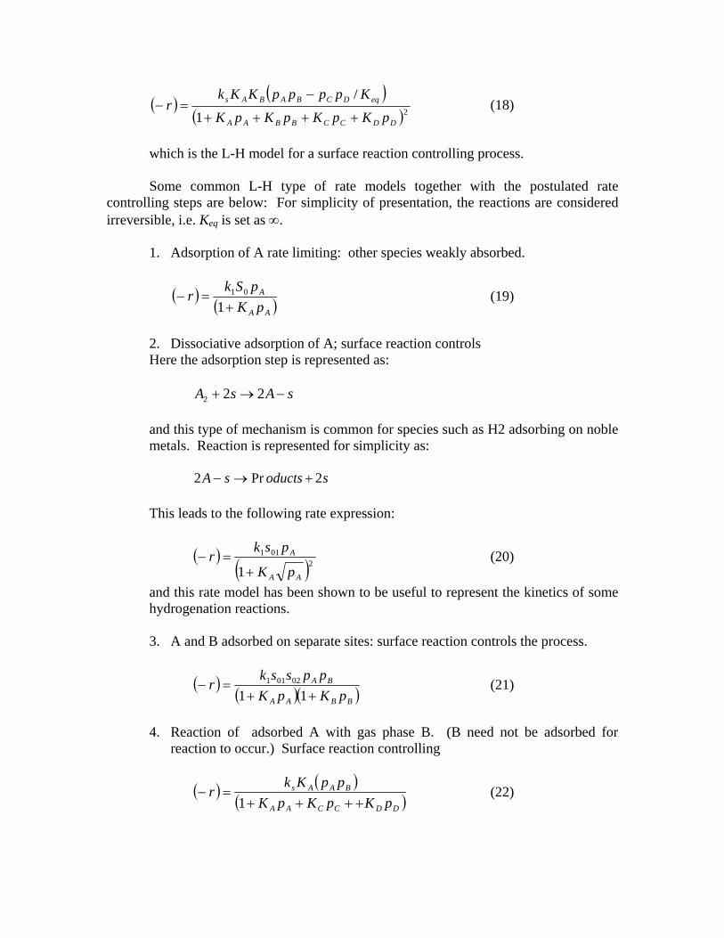
which is the L-H model for a surface reaction controlling process. Some common L-H type of rate models together with the postulated rate

controlling steps are below: For simplicity of presentation, the reactions are considered irreversible, i.e. Keq is set as ∞.

1. Adsorption of A rate limiting: other species weakly absorbed.

( ) ( )AA

A

pKpSk

r+

=−1

01 (19)

2. Dissociative adsorption of A; surface reaction controls Here the adsorption step is represented as: sAsA −→+ 222

and this type of mechanism is common for species such as H2 adsorbing on noble metals. Reaction is represented for simplicity as: soductssA 2Pr2 +→− This leads to the following rate expression:

( ) ( )2011

1 AA

A

pK

pskr

+=− (20)

and this rate model has been shown to be useful to represent the kinetics of some hydrogenation reactions. 3. A and B adsorbed on separate sites: surface reaction controls the process.

( ) ( )( )BBAA

BA

pKpKppssk

r++

=−11

02011 (21)

4. Reaction of adsorbed A with gas phase B. (B need not be adsorbed for

reaction to occur.) Surface reaction controlling

( ) ( )( )DDCCAA

BAAs

pKpKpKppKk

r++++

=−1

(22)

Note that the denominator is to the power one now representing the fact that this is a single site mechanism. KC = KD = 0 if products are not adsorbed. A model of this type is used in selective catalytic reduction.

Power law vs L-H Models

Characteristics of the L-H can be examined by considering a simple case. Assume that only the species A is strongly adsorbed and the reaction is irreversible. Assume B is in excess and a dual site mechanism. This leads to the following simplified rate model:

( )( )21 AA

AAs

pKpKk

r+

=− (23)

The rate constant ks increases with temperature while the adsorption equilibrium

constant KA generally decreases with temperature. The net effect may be such that the rate reaches a maximum at a particular temperature. This can not be predicted by power law model. Another observation is the dependency on concentration. For low concentration, the reaction would be seen as a first order while for high concentration, a negative first order dependency may be observed. For other complex schemes, the rate can reach a maximum at an intermediate coverage of, say B, in a bimolecular reaction A+B to products. The advantage of the power law models are their simplicity. This is especially useful if one needs to include the transport effects and use them in a reactor model. Also simple power law models are often found to fit the data well even for the case where L-H models have been fitted. Two different mechanisms L-H may produce similar rate models and model discrimination can often be difficult. Microkinetic Models The model is built using elementary reactions that occur on the catalytic surface and their relation with each other and with the surface during the catalytic cycle. The major advantage is implementation of surface bonding and correlation of surface structure with semiempirical molecular interaction parameters. Another advantage is that the rate constants for similar types of reaction can be estimated by molecular considerations and extrapolated to a wider class of similar types of reactions. Rate constants for individual elementary reactions can be measured independently and these can be used in the overall scheme. One limitation of this approach is that the rate expressions cannot be often obtained analytically. Numerical solutions are needed but the resulting equations are often stiff due to the wide range of time constants for the various elementary steps. An example of a microkinetic model for catalytic oxidation in a three way converter (TWC) is shown in Table 1 from the work of Koci et al. The catalyst was Pt/Ce/γ-Al2O3 and the process involves CO oxidation, hydrocarbon oxidation and NOx

reduction. (Hence the terminology three way converter). The scheme is illustrative of the complex multi-step nature of catalytic process.

Surface Interaction Models Experimental methods, namely NMR, spectroscopy, and kinetic measurements are available to study the surface topology of catalysts, the adsorption sites and how the molecules are adsorbed on the catalyst surface. Unfortunately these experiments are very difficult to perform and most of the time, there is a high discrepancy between different techniques. Computer simulations, therefore are becoming increasingly popular to study the structure and the transport behavior of the catalysts. The two commonly used simulation techniques to study the structural and dynamical properties include Molecular Dynamics (MD) and Monte Carlo (MC) simulations. MD has been extensively used to study dynamic and equilibrium properties of different adsorbates in different catalysts. In MD simulation, Newton’s equations of motion are solved for each molecule. Since the continuous motion of the molecules is approximated by discrete movements in time, MD simulations are deterministic. The time step used in the calculations is usually between 5-10 fs resulting in practical simulation times up to 10 ns with current computers. MC simulation, on the other hand is a probabilistic method. Many useful information such as energetics of the individual adsorption sites, adsorption isotherms and related thermodynamic properties properties can be obtained by MC simulations. More information about these techniques can be found at [1]. MC simulations are also used to study surface reactions. Much effort has been focused on study of reduction reaction of NO by CO since this is a very important reaction in pollution control in catalytic converters. This reaction is very sensitive to the metal substrate used as a catalyst and to the type of the surface[3]. The MC algorithm involves randomly selecting an event from the given mechanism with a probability based on the reaction rate constants. Usually 106 MC steps are attempted to reach stability in the results. Cortes et al [2] studied this reaction over the Rh catalyst. The authors found that there is a good agreement between the MC simulations and the analytical solutions of Langmuir-Hinshelwood mechanism. Korluke et al [3] developed a simple lattice gas model to study the effect of molecularly adsorbed NO using MC simulations. The authors found that NO and CO desorption is necessary for a steady-state reaction. The problem with these simulations is that the texture of the porous catalyst might be too complex for realistic representation. Many simplifications are made in the modeling. Still, the simulations provide a lot of information about the surface reactions, and structure and properties of surfaces. Simulation results can be used in microkinetic model which can then be used to construct more realistic L-H models. Thus the three modes together provide a hierarchy for multi-scale analysis. Kinetic Model: Examples

1. SCR A mechanism proposed is adsorption of NH3 on active sites followed by reaction with NO in the gas phase.

kf sNHsNH g 3)(3 ↔+ K=kf / kb

kb

OHNOgNOsNH k2223 4

641)( +⎯→⎯++

Step 2 is assumed to be rate controlling. Then

( )(NOsNHkr 3= ))

( ) (sNHKsNH g33 =

Rate is therefore equal to ( ) ( ) sNHNOkK gg 3 A site balance gives

03 ssNHs =+ or ( ) 03 ssNHKs g =+

( )( )gNHKs

s3

0

1+=

Hence the proposed kinetic scheme is

( ) ( )( )g

gg

NHKNHNOkKs

r3

30

1+=

Reaction Engineering Issues

In this section, we indicate the main reaction engineering problems associated with gas-solid reaction. The modeling tasks can be divided into two categories:

i. Particle scale modeling

Since the catalyst is generally porous, intraparticle diffusion becomes an important rate limiting factor. Thus, one needs to consider the diffusion in the pores of the catalyst with simultaneous chemical reaction. In case of monolithic type of catalyst, particle scale modeling is replaced by modeling of surface adsorption, desorption and reaction processes.

ii. Reactor scale modeling

The reactor scale modeling consists of writing the mass and heat balances for the reactor including flow non-idealities, if any. The particle scale model becomes a sub-model here and provides the necessary expressions for the rate of reaction.

Reactor Models Coupling with Particle Models: In order to see the coupling of reactor models with particle model it is useful to

consider a packed bed reactor which is modeled as a plug flow reactor. Also isothermal conditions are considered first. Consider a differential element of reactor change in molar flow rate if I is given as:

( )ratedefinetousedmeasureRF ii ×=∆

A mass balance leads to:

( ) ∑=−= jjiiBi rvR

dxdN

ε1

Also iti yNN =

RT

PQN G

t =

where Ri is the rate of production of species i per unit catalyst volume. Hence the factor ( )Bε−1 appears in the rate term on RHS. Since gigi cuN = the equation can be written as:

( ) iBg

igig

g Rdx

duc

dxdc

u ε−=+ 1,,

If change in the gas velocity is small (e.g. dilute systems) then

( ) ( )∑−=−= jjiBiBig

g rvRdx

dcu εε 11,

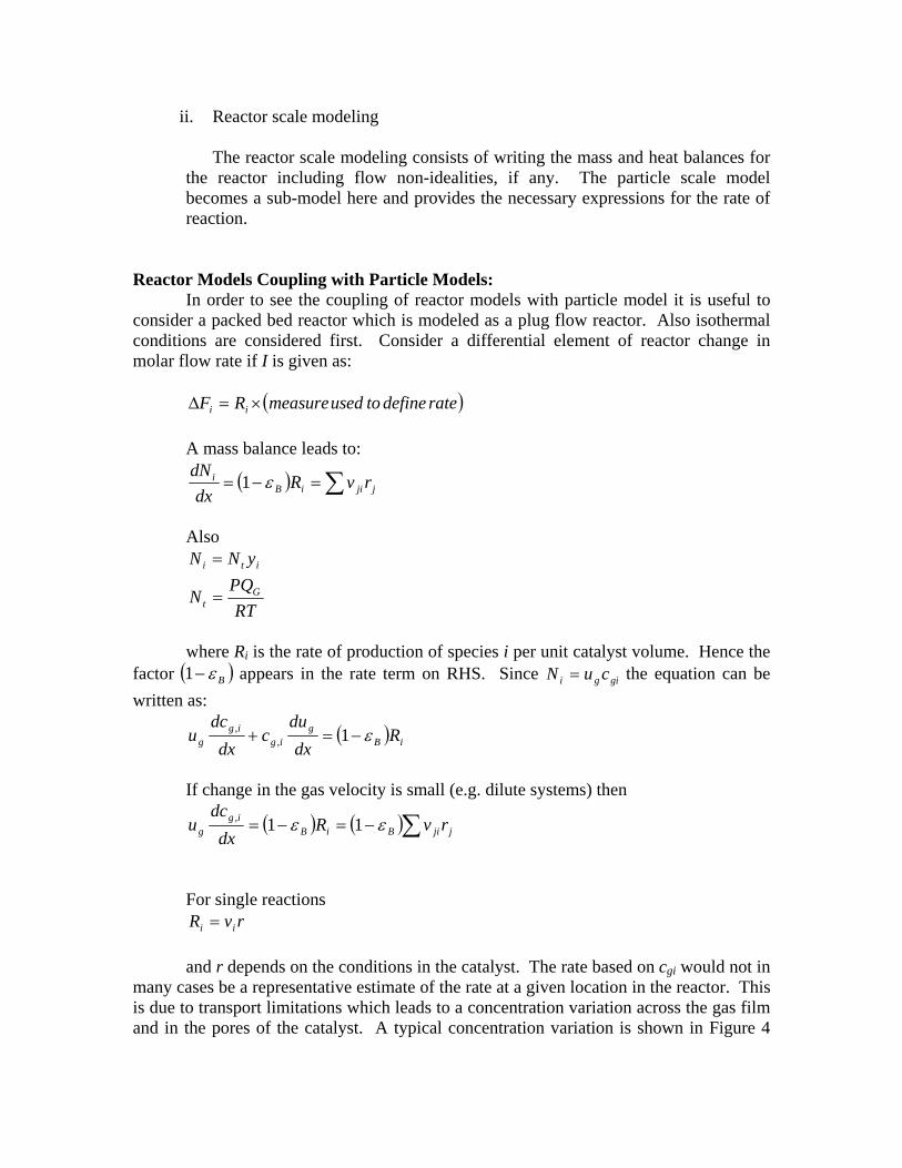
For single reactions rvR ii = and r depends on the conditions in the catalyst. The rate based on cgi would not in many cases be a representative estimate of the rate at a given location in the reactor. This is due to transport limitations which leads to a concentration variation across the gas film and in the pores of the catalyst. A typical concentration variation is shown in Figure 4

and the role of the particle scale models is to take into account these variations to find a representative rate. Internal diffusion

Local boundary layer around a particle

Cs

Cgi(0) Cgi(l)

Cgi

catalyst

Note that similar profiles exist for temperature. For single reaction and dilute systems, we have the following equation for each species i.

( ) ( ) rvRdx

dcu iBiB

igg εε −=−= 11, (1)

r = rate of reaction including transport effects, i.e. including the effect of point to point variation of concentration in the catalyst. Let ~ ( )gig Tcr ,, be the rate based on bulk conditions. Ratio of r to r~ is called effectiveness factor and is of great convenience in modeling heterogeneous systems. Eq. 1 becomes

( ) ( ηε gigiBig

g Tcrvdx

dcu ,1 ,

, −= ) (2)

In general, η is a function of cg,i and Tg. Only for first order isothermal case η can

be found independently as shown later. Solution of Eq. (2) is done numerically for multiple species and multiple reactions. The procedure is similar to that homogeneous reactions with a major difference that at each integration step η0 need to be computed by a “particle model” based on the local values of gas phase concentrations and temperatures. Particle models are considered in detail in the following section. Particle Models

1. Models for internal diffusion

The particle scale effects are usually modeled by the diffusion-reaction equation. More detailed models using Stefan-Boltzmann equations are not considered here. The diffusion in a porous catalyst is characterized by an effective diffusivity, De,i with i indicating the species. The transport of species i within the pore structure is then governed by the following equation for a spherical catalyst

( ) ( )∑ <<+−=∇ RrrrarCD jjjjiiei 02 υ (1) where the quantities used are defined as follows:

2∇ = Laplacian which takes the following form for a spherical catalyst. 2∇ =

rr

rr1 22 ∂

∂∂∂

r = Radial position R = Radius of the catalyst

i,eD = Effective diffusivity of species i in the pores of the catalyst; Model assumes the same diffusivity for the poisoned and unpoisoned zones.

jiυ = Stoichiometric coefficient of species i in the j-th reaction rj = rate expression of j-th reaction per unit total volume of catalyst.

( )ra j = Activity of the catalyst for the j-th reaction; Note the radial dependence of the activity profile. This quantity may change with time as the catalyst gets progressively poisoned.

The boundary conditions needed to solve Eq. (1) are as follows:

at 0r

C,0r i =

∂∂

= (2)

at ( ii,gi,e

i,gi CCDk

rC

,Rr −=∂

∂= ) (3)

where is the gas film mass transfer coefficient for the i-th species. i,gk Cg,i = concentration of species i in the external gas phase near the particle under

consideration. Again kg,i is based on concentration driving force. Various definitions are used for kg and units should be used carefully. The solution of Eq.(1) gives the detailed concentration profiles in the particles. From the solution, an average rate can be calculated and used to find η0 . This forms the basis for the particle model.

First Order Reaction

The intraparticle diffusion models simplify for a first order kinetics. For this case,

the results can be obtained analytically. The first order kinetics is often a good approximation in oxidation reactions. The oxygen is usually present in excess compared to the pollutants. For such cases, the kinetics can be simplified to a first order kinetics:

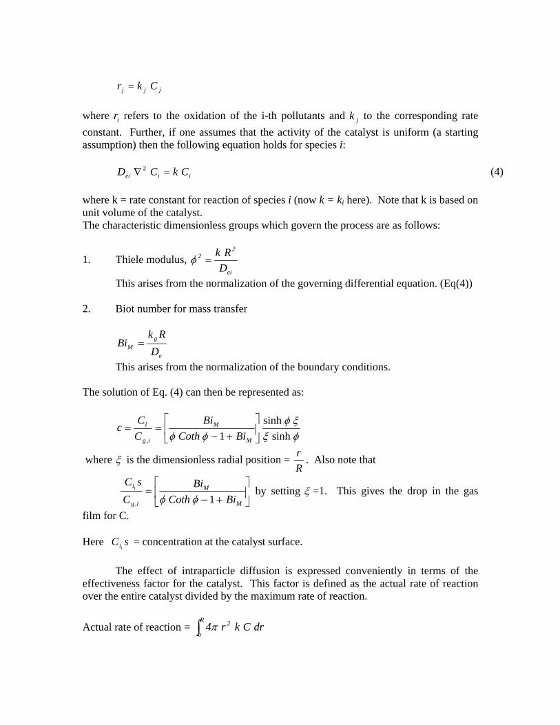
jjj Ckr = where refers to the oxidation of the i-th pollutants and to the corresponding rate constant. Further, if one assumes that the activity of the catalyst is uniform (a starting assumption) then the following equation holds for species i:

ir jk

(4) iiei CkCD =∇ 2

where k = rate constant for reaction of species i (now k = ki here). Note that k is based on unit volume of the catalyst. The characteristic dimensionless groups which govern the process are as follows:

1. Thiele modulus, ei

22

DRk

=φ

This arises from the normalization of the governing differential equation. (Eq(4)) 2. Biot number for mass transfer

e

gM D

RkBi =

This arises from the normalization of the boundary conditions. The solution of Eq. (4) can then be represented as:

φξξφ

φφ sinhsinh

1,⎥⎦

⎤⎢⎣

⎡+−

==M

M

ig

i

BiCothBi

CC

c

where ξ is the dimensionless radial position = Rr . Also note that

⎥⎦

⎤⎢⎣

⎡+−

=M

M

ig

i

BiCothBi

CsC

1,

1

φφby setting ξ =1. This gives the drop in the gas

film for C. Here = concentration at the catalyst surface. sCi1

The effect of intraparticle diffusion is expressed conveniently in terms of the effectiveness factor for the catalyst. This factor is defined as the actual rate of reaction over the entire catalyst divided by the maximum rate of reaction.

Actual rate of reaction = ∫R

o

2 drCkr4π

Maximum rate of reaction = g

3CkR

34 π

Note the species subscript, i, has been dropped for convenience. The actual rate of reaction can also be expressed as:

2Actual Rate 4 en R

CR Dr

π=

∂⎛ ⎞= ⎜ ⎟∂⎝ ⎠which is a simpler form to calculate.

The expression for the overall effectiveness factor oη is then obtained as:

( ) ( )M

M

BiBi

+−−=

1coth1coth3

2 φφφφ

φη

Also the following limiting case when ∞→MBi should be noted

( 1coth32 −= φφ

φηc ) which is also referred to as the internal effectiveness factor.

The above expression is suitable for a spherical catalyst. For catalyst of other

shapes it is convenient to use a “shape normalized” Thiele modulus defined as

21

⎟⎟⎠

⎞⎜⎜⎝

⎛=Λ

ep

p

Dk

SV

where is the volume of the catalyst and is the external surface area of the catalyst.

Note that

pV pS

3φΛ = for a sphere.

An approximate expression for effectiveness factor for all shapes is given by:

Λ

Λ≈

tanhcη

This is based on a slab model for geometry of the catalyst assuming there is no gas side resistance. In the limit of large Λ , we can use η as the reciprocal of Λ since the 1 for large Λ . The concentration profiles in a slab catalyst for various values of is shown in Figure 5.

→ΛtanhΛ

FIGURE MISSING Application problems to ascertain the importance of pore diffusion are illustrated by the following examples.

Problem 1: Rate for larger size given kinetics

Rate of reaction over a finely crushed catalyst of radius of 0.5mm was measured as 10.0 mole/sm3catalyst.

Temperature is 400 K and pressure is 105 Pa and mole fraction of reactant in the gas is 0.1. Find the rate for a catalyst of pellet radius of 3mm. Solution: Assume ηc=1 for small catalyst.

3

5

007.3400314.8

101.0mmol

RTyPCAg =

××

==

AgkCRate = Hence AgC

Ratek = smmolsmmolk 3256.3

/007.3/10

3

3

==

To find rate for larger catalyst, we need an estimate of intraparticle diffusion coefficient. Let De = 4x10-6 m2/s (a reasonable estimate). Then,

9118.03

==eD

kRφ

7051.0=cη

smmolekCRate Agc3/05.7== η

Diagnostics: The Weisz Model Given the measured rate, establish if there is significant pore diffusion resistance.

( )eAg

obsAW DC

RLModulusWeiszM

−==

2

where L = R / 3 = characteristic length scale If Weisz modulus (Wagner modules) < 0.15, then the concentration profile in the pellet is nearly uniform. Note that

roblem 2: Test for pore resistance d for a gas concentration of A of 20 mole/m3. The

catalyst particle diameter is 2.4 mm.

2φηcWM = PA rate of 105 mole/hr m3 cat is observe

An independently measured value is needed to solve this problem.

et us assume effective diffusivity is 5x10-5 m2/hr.

= R / 3 = 4 x 10-4 mm

agner modulus =

Strong pore resistance

he measured data are not representative of true or “intrinsic” kinetics.

roblem 3: Intrinsic kinetics

L Is there a strong pore diffusion resistance? Solution: L W

T PIn Problem 2, find the effectiveness factor and the true rate constant. Solution:

AgCkrate η=

15000 −== hrCratek

Ag

η

Since h depends on k, we used a trial and error solution. We expect h to be small. Let us assume some value, say 0.01.

=5000/η Thiele η equation

Then

η assumed kv

0.01 5x105 40 0.025 0.03 1.67x105 23 0.0433 0.063 7.93x104 15.9 0.0627

( )16

2

=−

= obsAT

RLM

AgeCD

55000×==k 105

ηV

mod = LulusThiele 40=e

V

Dk

025.0tanh==

φφη

Design Considerations Monolith Models Gas phase balanc

Ω∆=∆

here r = rate of reaction, single reaction case = measure used to define the rate per unit reactor volume

e Q Vrvc igiG

w

Ω For multiple reactions, vir is replaced by ∑ ji rv j where j is the reaction index.

ash-coat case lls of th

= surface area per unit volume of monolith

Wr based on external surface area of the wa e monolith Ω

xAV c∆=∆ Ac = cross sectional or frontal area

gc

L uA

= = gas superficial velocity Q

Ωrv =dx

dcu i

gig

If r is based on bulk concentration we have the pseudo-homogeneous model. If r is based on actual concentration, use effectiveness factor

( )Ω= gLgigi

g ccrvdx

dcu ,...,1η

To find η , balance transpor to surface and reaction at the surface.

t

( ) ( )siisigimi

Solve fo ccrvcc −=− for each species. (A)

r k

si. Find r(csi).

( )( )gi

si

cr=η

cr

Note that varies with x in laminar flow. Hence these calculations are to be repeated for each incremental position in x.

Alternate formulation is in terms of transfer rate to the walls. (similar to that in

km

Wendt’s paper) Here η is not explicitly calculated. Both cgi and csi are treated as variables. We will look at this formulation now.

Gas phase balance =∆ giG cQ - transferred to walls = ( )sigimi ccVk −Ω∆−

where Ω = surface area of the walls per unit reactor volume

( )sigimigi cck

dx−Ω−= for gu i = 1 to N

dc

( ) ( )siisigimi crvcck −=−

Both of these equations are solved simultaneously. Note that this is a differential algebraic system. Both methods are equivalent. Computation of η is simple for a first order reaction. Here Eqn. (A) reduces to

( ) ( ) sisisigimi ckcrcck ==− (B) where vi is taken as –1 for the key reactant. Eliminating csi

1

11−

⎥⎦⎣ simi kk⎤

⎢⎡

+= gic r

simi

simigiactual kk

kkcr

+=

simi

mi

kkk+

=η

The reactors are operated often in laminar flow. The transfer coefficient kmi can then be predicted by detailed 2-D models for diffusion and flow.

alculation of η for two components reacting with each other is slightly complicated. CEqn. (B) is now written for both components.

( ) 2121111 sssgm cckvcc −=− or other rate form k( ) 2122222 sssgm cckvcck =− −

21

21

gg

ss

cccc

=η

Equations have to be solved simultaneously for cs1 and cs2. Then η can be computed. Note that η varies along the reactor since the concentrations cs1 and cs2 also vary along

the reactor xial position. The calculation procedure for local values of a η is illustrated in the followi example.

SCR. Rate of transport of NOx (denoted as species 1) is:

ng Example: Consider a bimolecular reaction.

productsvNHNOx →+ 3 where v = 2/3 x This is representative of

( )sgm cckr 111 −=

111

msg k

rc =− c

111

mgs k

cc r−=

Rate of transport of NH3 is:

( )sgm cckvr 222 −=

222

msg k

vrcc =−

222

mgs k

cc −= vr

Rate of reaction is sss cckr 212=

⎟⎟⎠

⎞⎜⎜⎝

⎛−⎟⎟

⎠

⎞⎜⎜⎝

⎛−=

22

112

mg

mgs k

rckrckr

ate is often expressed in terms of an effectiveness factor R

ηggs cckr 212= Substituting and rearranging, an expression for η is obtained:

⎟⎠

⎜⎝

⎟⎠

⎜⎝ 21 mm kk

⎟⎞

⎜⎛

−⎟⎞

⎜⎛

−= 1222 11 gsgs cvkck ηηη

he effectiveness factor is now a function of local gas phase concentration.

Design Parameters 1. Binary Diffusivity in Gas Phase.

inary diffusion coefficient for a pair of gases denoted as 1 and 2 can be calculated by

T

Busing Lennard-Jones potential model. The equation suggested by Hirschfelder, Bird and

potz is: S

PMM

T1086.1DD

D2

12

212112 Ωσ

+×==

1

T is the absolute temperature, P is the absolute pressure in atm, and are the molecular weights. The two Lennard-Jones parameters are

1237−

where 1M 2M

12σ the collision diameter angstroms and DΩin the collision integral for diffusion. These values are usually

he quantity 12σtabulated. T is calculated as the average:

( )2112 21 σσσ +=

The collision integr are function of a parameter alsε

kT . This is calculated from the

1ε 2εvalues of and for each gases as:

kkk

NOTE: k = Boltzmann constant

2112 εεε=

xample: Estimate diffusion coefficient of CO in air at 800k and 1 atm.

the tables of Lennard-Jones force constants we find the following values:

E From Kk inε , Ain σ

O 110 3.590 Air 97 3.617 C

( )

( ) ( )

745.729.103

800Tk

29.103= 11097k

6035.321

12

12

12

==

=

==

ε

ε

σσ

rom the table of collision integrals, the value of

21 + σ

DΩF is 0.77.

Substituting into the formula

( )

( ) ( ) ( )sm101.1

177.06035.3291

2818001086.1

D24

2

21237

12

−

−

×=

⎟⎠⎞

⎜⎝⎛ +××

=

2. EFFECTIVE DIFFUSION COEFFICIENT

he diffusion within the catalyst proceed by two mechanisms: (1) Bulk diffusion within

he bulk phase diffusivity is corrected for internal pore diffusion by incorporating two

Tthe pores(2) bombardment with the walls of the pore if the pore radius is small. The second mechanism is know as Knudsen diffusion. Tfactors (1) porosity, ε which accounts for the reduced area accessible for diffusion and (2) tortuosity, τ which accounts for the non-straight path for diffusion.

τε

12eff,12 DD =

The Knudsen diffusion coefficient depends on the average radius of the pores and is given by:

KeffK DDτε

=,

Where is the Knudsen diffusivity in a single cylindrical pore.

nudsen diffusion occurs when the size is the pores of the order of mean free path of the

here is the Knudsen diffusion coefficient given as:

KD Kdiffusivity molecule. w KD

1eK Vr32D =

er = effective pore radius and is the average molecular speed of species 1. This is

gi

1V ven by:

21

11 M

RT8V ⎟⎟⎠

⎞⎜⎜⎝

⎛=

π

Substituting the values of gas constants, we find the following dimensional equation for the Knudsen diffusion coefficient.

21

1e1,K M

Tr97D ⎟⎟⎠

⎞⎜⎜⎝

⎛=

in sm2 with in m and T in Kelvins. er The phenomena of ordinary diffusion and Knudsen diffusion, may be occurring simultaneously. The two can be combined by the following formula:

eff,Keff,12eff,1 D

1D

1D

1+=

Additional mechanism is the surface diffusion where the adsorbed species migrates along the surface. The effects are often ignored if the pores are relatively large. This phenomena may be of importance in monolith type of catalysts. EXAMPLE: Calculate the effective diffusivity of CO in porous alumina catalyst whose physical characteristics are as follows: Porosity = 0.8. Average pore diameter = 1 µm.

( ) sm1012.21006.10.48.0DD 254

12v

eff,12−− ×=×==

τε

where is taken as the value for a CO-air mixture at 800 K, 1 atm. 12D

( ) ( ) ( ) ( ) ( )( ) ( )

( ) ( ) ( ) sm1004.1sm778m100.48.032D

sm778kmolkg28

N/smkg1JmN1K800KkmolJ10314.88

MRT8

m10m1r

r32D

246eff,1K

2123

21

1

6e

1ev

eff,1K

−−

−

−

×==

=⎭⎬⎫

⎩⎨⎧ ×

=

⎟⎟⎠

⎞⎜⎜⎝

⎛=

==

=

π

πν

µ

ντε

Then, the effective diffusion coefficient is:

sm1076.1D

1004.11

1012.21

D1

D1

D1

25eff,1

45eff,1Keff,12eff,1

−

−−

×=×

+×

=+=

GAS SIDE MASS TRANSFER COEFFICIENT The external mass transfer coefficient from a spherical particle is correlated by the following dimensionless equation 3121 ScRe69.02Sh += where

Sh = Sherwood number = gp

kd

D

Re = Reynolds number = pg d

Uυ

gU is the linear velocity of the gas on the bulk stream.

Sc = Schmidt number = Dυ

The corresponding value for the heat transfer coefficient can be obtained by using the analogy between heat and mass transfer. The above correlation can be used for heat transfer with Nusselt and Prandtl number substituting the Sherwood and Schmidt terms. An alternate correlation recommended by Whitaker is: ( ) 4.03221 PrRe06.0Re4.02Nu ++= INTERNAL FLOW

Mass and heat transfer coefficient for flow through internal ducts are needed for the design of monolith catalysts. For this case the correlation for laminar flow in a circular pipe is used but the channel diameter is replaced by the equivalent hydraulic diameter. For pipe flow, the following correlation is useful for laminar flow

( )32

PrRe04.01

PrRe065.066.3

⎥⎦⎤

⎢⎣⎡+

+=

LD

LDNu

Equation is valid for Re < 2300 and assuming a constant wall temperature. Note that the Nu reaches the asymptotic value of 3.66. The thermal entry length (a point at which the Nusselt number reaches the asymptotic value) is given by the following expression.

PrRe017.0DLeh =

For other geometry the concept of hydraulic diameter can be used.

Hydraulic diameter = perimeter Wetted

section cross of Area⋅4

The asymptotic Nusselts number for various geometries are shown below: TABLE 2: Nusselt numbers and the product of friction factor times Reynolds number

for fully developed laminar flow in ducts of various cross-sections.

hDNu Cross Section Constant Axial

Wall Heat Flux Constant Axial

Wall Temperature hDRef

3.1

2.4

53

4.364

3.657

64

3.6

2.976

57

8.235

7.541

96

Equilateral Triangle

Circle

Square 11

An examplgiven belowEXAMPLE

A reactor wThe walls aof 0.070 m/exhaust gas0.187%. Assume fullimiting val

DCO

Equ

∞

e problem to estimate the effect of mass transfer in monolith arrangement is .

alls consist of passages which are square in cross section with 1 mm sides. re coated with a catalyst which oxidizes CO with the surface reaction constant s at 800K. The pressure is and the mean molecular weight of es is 29. Calculate the CO reduction at a location where CO mole fraction is

Pa1015.1 5×

ly developed profile for mass transfer. Then from the Tables we find that ue of Sherwood number is 2.98.

secm101.1 24air

−− ×=

( ) ( ) mm1LL4L4 2

===diameter ivalent

secm0298.0

101101.1x98.2k

98.2Ddk

3

4

x

hx

=×

×=

=

−

−

The surface reaction rate constant is secm070.0 . The overall rate constant is obtained by

adding the two resistances in series

secm021.0

k1

k1k

1

ss

=⎥⎦

⎤⎢⎣

⎡+=

−

Mass transport contributes 70% resistance (verify). The rate of CO oxidation is then given as follows:

( ) ( )

3

5

24

15800314.8

101sec

315.0109.55.1021.

mmole

RTPC

mmolegyCkR

bulk

CObulk

=×

×==

=×== −

PACKED BEDS For flow of gases in packed beds, an appropriate correlation for heat transfer coefficient is ( ) 313/221 PrRe2.0Re5.0Nu +=

Note: ug = superficial velocity = cA

mρ&

cBB

gg A

muV

ρεε&

== = interstial velocity

Re is defined as µ

ρVL

RhLNu =

The pressure drop in packed bed is usually calculated from the Ergun equation

L

VL

VdxdP gg

2

2

75.1150 ρµ+=

where L is a characteristic length parameter defined as:

⎟⎟⎠

⎞⎜⎜⎝

⎛−

=B

B

1dpL

εε

The first term in the Ergun equation accounts for the viscous drag while the second term accounts for the form (inertia) drag.

For non-spherical particles, use p

pp A

Vd

6= , i.e. an equivalent diameter.

Matlab Solutions to Diffusion-reaction problems See pdf file on web. -=----------------------------------------------------------------------------- References:

1. M.P. Allen, D.J. Tildeslay, Computer Simulation of Liquids (Clarendon, Oxford, 1987)

2. J. Cortes, E. Valencia, J. Phys. Chem. B. 2004, 108, 2979-2986 3. O. Korluke, W. von Niessen, Surface Science, 401 (1998) 185-198