Proceedings World Geothermal Congress 2010 Bali, Indonesia, 25-29 April 2010

1

Gas Chemistry of Volcanic Geothermal Systems

Stefán Arnórsson1*, Erlindo Angcoy2, Jón Örn Bjarnason1, Niels Giroud1, Ingvi Gunnarsson3, Hanna Kaasalainen1, Cyrus Karingithi4 and Andri Stefánsson1

1Institute of Earth Sciences, University of Iceland, Sturlugata 7, Reykjavík, Iceland 2Energy Development Corporation, Energy Center, Merritt Road, Fort Bonifacio, Taguig City, Philippines

3Reykjavík Energy, Baejarháls 1, Reykjavík, Iceland 4Kenya Electricity Generating Company, Stima Plaza, Phase III, Kolobot Road, Parklands, Nairobi, Kenya

*sted@raunvis.hi.is

Keywords: Geothermal systems, magma gases, gas fluxes, gas equilibria, aquifer fluid composition, aquifer fluid vapor fraction.

ABSTRACT

This article focuses on quantifying the processes that govern the concentrations of the major reactive gases (CO2, H2S, H2 and CH4) in fluids in aquifers producing into wet-steam wells in the volcanic geothermal systems of Olkaria (Kenya), Mahanagdong (Philippines) and Nesjavellir, Hellisheidi and Krafla (Iceland). Many of the wells in these areas have “excess” discharge enthalpy (higher than that of vapor-saturated liquid at the aquifer temperature). In two of the wells at Krafla the elevated enthalpy is to a significant extent due to the presence of vapor in the initial aquifer fluid. In general, however, excess enthalpy is mostly caused by segregation of vapor and liquid during their flow through the depressurization zone around discharging wells. The concentrations of H2S and H2 in the initial aquifer liquid are controlled by close approach to equilibrium with specific hydrothermal mineral assemblages. Aquifer liquid CO2 concentrations at Olkaria are also controlled by such equilibria but in the other fields by their supply to the geothermal fluid. The initial aquifer fluids at Hellisheidi and Olkaria contain on average 0.5% and 0.03% vapor by weight, respectively. The vapor content of the aquifer fluid at Nesjavellir and Krafla is considerably higher, on average 0.9% and 1.2%, respectively, if we exclude two of the Krafla wells that have vapor-dominated aquifers in terms of vapor volume (5.6 and 9.6% vapor by weight). A few wells in all these areas discharge slightly degassed fluid due to steam loss in the producing aquifers. The large scatter of the H2 data from Mahanagdong makes estimation of vapor fractions in producing aquifers unreliable. When taking into account the estimated vapor fraction in the aquifer fluids, results indicate that equilibrium between H2, CH4 and CO2 is closely approached at around 300°C and that departure from equilibrium increases with decreasing temperature.

1. INTRODUCTION

Gases are often major solutes in fluids of volcanic geothermal systems, in particular CO2, H2S and H2, but in some systems CH4 may also be present in abundance. The gas composition of fluids discharged from wells drilled into these systems provides important information about various features of these systems (e.g. D´Amore and Panichi, 1980; Giggenbach, 1980; D´Amore and Truesdell, 1985; Arnórsson et al., 1990; Gudmundsson and Arnórsson, 2002). Changes with time in the gas content of well discharges of producing geothermal reservoirs provide valuable information about the response of the reservoir to the production load, such as cold recharge and enhanced boiling (e.g. Gudmundsson and Arnórsson, 2002; Kissling

et al., 1996; Ármannsson, 2003). Environmentally important gases (CO2, CH4, H2S) are not only released into the atmosphere from magma during volcanic eruptions, but also when it solidifies underground to form intrusive bodies. A geothermal system above cooling magma may behave as essentially open to the escaping magma gases or act as a trap due to gas-gas and gas-mineral reactions that consume these gases. An understanding of these reactions is important for evaluating the role of utilized as well as undeveloped geothermal systems in the long-term transfer of magma gases into the atmosphere.

The present contribution focuses on explaining the chemistry of the major reactive gases in fluids of several volcanic geothermal systems in different geological environments.

2. THE STUDY AREAS

The geothermal fields considered in the present study include Olkaria in Kenya, Mahanagdong in the Philippines and Krafla, Nesjavellir and Hellisheidi in Iceland. The two last mentioned fields represent production wellfields of the Hengill geothermal area. Olkaria is located within the Eastern Rift Valley of Kenya. The dominant rock types are trachytes with less abundant basalts and rhyolites. The latest volcanic eruption at Olkaria occurred about 250 years ago producing a comendite lava flow. The Mahanagdong geothermal field in the Philippines is associated with a subduction zone. It hosts andesitic rocks. The latest exposed volcanics formed in late Pleistocene times (e.g. Herras et al., 1996). The Icelandic fields occur in a divergent zone and basaltic rocks. At Hellisheidi and Nesjavellir the latest volcanic eruptions occurred around 1,000 and 1,900 years ago, respectively. At Krafla the last two volcanic episodes took place in 1724-1746 and 1975-1984. During the latest volcanic episode at Krafla, a sharp increase in the gas content of fumarole steam occurred, particularly in CO2, as well as in the discharges of the wells that had been drilled at that time (Ármannsson et al., 1982) but since then the magma gas pulse has declined much (Gudmundsson and Arnórsson, 2005).

The fields considered in the present study are all liquid-dominated. They are all being exploited and many wells have been drilled in each of them. Subsurface temperatures exceed 300°C in all of the areas. Some of the wells have liquid enthalpy but most have considerable excess enthalpy, i.e. the enthalpy of the discharge is significantly higher than that of steam-saturated water at the aquifer temperature.

The chemistry of the fluids discharged from wells shows much variation between areas. There is also some variation

Arnórsson et al.

2

between wells in the same wellfield. Representative analyses are shown in Table 1.

3. THE STRUCTURE AND EVOLUTION OF VOLCANIC GEOTHERMAL SYSTEMS

The term volcanic geothermal system is considered to be synonymous with geothermal systems in young igneous environments by the classification of Goff and Janik (2000) and high-temperature systems by the classification of Bödvarsson (1961). Likely the heat source to many of these systems is magma intruded into their roots. It may be a single major magma body that is replenished at intervals by new magma from deeper crustal levels or the mantle. Alternatively, the intrusive heat source may consist of a complex of relatively small bodies intruded over a period of time, including sheeted dyke complexes at diverging lithosphere plate boundaries.

Every volcanic geothermal system has its birth, evolution and extinction. In Iceland, which lies astride a diverging plate boundary, volcanic geothermal systems are in the end disconnected from their magma heat source by the process of crustal accretion and when this occurs they begin to cool down. The same is likely the case in Kenya because crustal rifting is active in the Rift Valley. On converging plate boundaries the situation may be more complex.

During the early lifetime of a volcanic geothermal system convecting hydrothermal fluid will transport heat from the cooling magma to higher levels in the crust. When the heat source becomes extinct, either due to a shift in the position

of the conduit of the rising magma, or by drifting of the geothermal system from this source, we are left with a body of hot rock and hot fluid whose energy is no longer replenished. Gradually, this hot body that constitutes the geothermal system will cool down.

The natural heat output of some volcanic geothermal systems has been estimated reasonably accurately. To account for the estimated heat output, it is inevitable that the layer between magma and the base of the convecting hydrothermal fluid through which the magma heat is conducted must be very thin, a few hundred of metres, even less (Arnórsson et al., 2007).

Deep drilling in the Krafla geothermal field in Iceland has revealed a layer of superheated steam below a two-phase reservoir. Two drillholes have penetrated magma at 2-3 km depth. At Alto Peak in the Philippines, a core of vapor in the central part of the field is enveloped by a liquid-dominated reservoir (Reyes et al., 1993). This indicates that the convecting fluid at the deepest levels in some volcanic geothermal systems nearest to the magma may be vapor and the fluid at higher levels is, at least partly, steam-heated. The close vicinity of magma and hydrothermal fluid favors easy mixing of magma gases with that fluid.

While young, degassing of the magma heat source likely adds gases to the circulating hydrothermal fluid. These gases include H2O, CO2, H2S, SO2, H2, CO, HCl, HF and likely many more fugitive species. Some of these gases act like acids when dissolved in liquid water, such as SO2 and in particular HCl. Upon mixing they will turn the fluid acid.

Table 1. Representative analyses of samples of liquid water and vapor collected from discharges of wells in the study areas. Concentrations are in mg/kg for liquid samples and in mmoles/kg for vapor samples.

1 2 3 4 5 6 7

h d ,t 2140 1653 1071 1910 2400 1372 1403

Pd 5.5 2.5 13.0 15.5 17.0 9.5 11.4

T f 242 262 247 299 291 267 286 Liquid sample

pH/°C 8.95/20 8.67/20 9.03/20 8.40/19 8.11/22 9.13/17 6.08/24 SiO2 576 855 558 867 786 659 754 B 5.9 6.8 0.67 1.62 1.89 1.23 61.7 Na 526 1283 237 235 142 201 2551 K 83 208 34.5 53.9 31.4 32.7 516 Ca 0.56 0.66 2.65 1.56 0.30 0.35 38 Mg 0.010 0.070 0.004 0.0009 0.0053 0.0122 0.033 Al 0.79 0.67 1.55 1.67 1.64 1.74 0.307 Fe 0.02 0.02 0.014 0.0022 0.0011 0.011 0.089 CO2

a 92 2465 38.3 17.9 51.3 7.4 61.4 H2S

b 9.9 3.96 46.1 89.5 83.8 76.1 0.94 SO4 54 112 262.4 167.5 1.9 7.5 22.2 Cl 658 240 49.5 147.8 110.5 199 4396 F 64 105 1.05 1.38 1.16 1.10 1.57

Vapor sample CO2 55.0 4260 50.0 79.8 139.5 29.7 634.0 H2S 5.44 3.55 3.60 24.2 51.1 24.1 6.02 H2 3.55 1.05 6.96 24.4 41.45 10.80 1.04 CH4 0.44 0.833 0.518 0.045 0.414 0.045 1.253 N2 2.83 11.27 9.61 1.95 4.52 2.74 3.13 Ar - - 0.174 0.042 0.083 0.045 0.028

h d ,t : Discharge enthalpy (kJ/kg). Pd : Sampling pressure (bar abs.). T f : Aquifer temperature (°C) based on the results of the quartz and Na/K geothermometers. aTotal carbonate carbon as CO2.

bTotal sulphide sulphur as H2S. 1: Olkaria 15, 2: Olkaria 301, 3: Krafla 27, 4: Krafla 32, 5: Nesjavellir 21, 6: Hellisheidi 7, 7: Mahanagdong 16D. Numbers after local name indicate well number.

Arnórsson et al.

3

Table 2. Conservation equations for mass flow (M, kg/s), specific enthalpy (h, kJ/kg) and mole numbers of chemical components (m, moles/kg) used to calculate the composition of the initial aquifer liquid and vapor in the aquifer of wet-steam wells from analytical data on vapor and liquid samples collected at the wellhead. Superscripts: f = feed zone, t = total, l = liquid, v = vapor, e = intermediate zone, d = discharge. Subscripts r and s denote non-volatile component and gaseous species, respectively.

Table 3. Equations to calculate individual component concentrations in the initial aquifer liquid and vapor of wet-steam wells from analytical data on vapor and liquid samples collected at the wellhead.

Model Aquifer liquid Aquifer vapor

1 and 2 mr

f ,l =mr

d ,t

1− X f ,v ms

f ,v = msd ,t ⋅ X f ,v 1− 1

Dsf

⎛

⎝ ⎜ ⎜

⎞

⎠ ⎟ ⎟ +

1

Dsf

⎡

⎣ ⎢ ⎢

⎤

⎦ ⎥ ⎥

−1

3 mr

f ,l =mr

d ,t

1− X f ,v⋅ V f ,t 1− 1

1− X e,v

⎛

⎝ ⎜

⎞

⎠ ⎟ +

1

1− X e,v

⎡

⎣ ⎢

⎤

⎦ ⎥ −1

msf ,v =

msd ,t

V f ,t⋅ X f ,v 1− 1

Dsf

⎛

⎝ ⎜ ⎜

⎞

⎠ ⎟ ⎟ +

1

Dsf

⎡

⎣ ⎢ ⎢

⎤

⎦ ⎥ ⎥

−1

4 mr

f ,l =mr

d ,t

1− X f ,v⋅ h f ,t − h e,v

h d ,t − h e,v

⎡

⎣ ⎢ ⎢

⎤

⎦ ⎥ ⎥ ms

f ,v =ms

d ,t

V f ,t⋅ X f ,v 1− 1

Dsf

⎛

⎝ ⎜ ⎜

⎞

⎠ ⎟ ⎟ +

1

Dsf

⎡

⎣ ⎢ ⎢

⎤

⎦ ⎥ ⎥

−1

5a mr

f ,l =mr

d ,t

1− X f ,v⋅ V f ,t 1−

1

1− Z e,v

⎛

⎝ ⎜

⎞

⎠ ⎟ +

1

1− Z e,v

⎡

⎣ ⎢

⎤

⎦ ⎥ −1

msf ,v =

msd ,t

V f ,t⋅ X f ,v 1− 1

Dsf

⎛

⎝ ⎜ ⎜

⎞

⎠ ⎟ ⎟ +

1

Dsf

⎡

⎣ ⎢ ⎢

⎤

⎦ ⎥ ⎥

−1

6b

mrf ,l = mr

d ,t V f ,t (1− X f ,v )[ ]−1

msf ,v = ms

d ,t ⋅ X e,v (1−1

Dse

) +1

Dse

⎡

⎣ ⎢ ⎢

⎤

⎦ ⎥ ⎥ ⋅ X f ,v (1−

1

Dsf

) +1

Dsf

⎡

⎣ ⎢ ⎢

⎤

⎦ ⎥ ⎥

−1

⋅ V f ,t (1− X e,v ) ⋅1

Dse

−1⎛

⎝ ⎜ ⎜

⎞

⎠ ⎟ ⎟ +1

⎡

⎣ ⎢ ⎢

⎤

⎦ ⎥ ⎥

−1

For model 1, X f ,v is obtained from eqn. (1) and for model 2 from eqn. (2) by choosing gas s to be H2. For models 3 and 4, X f ,v

is obtained from eqn. (4), V f ,t from eqn. (11) and X e,v from (8). The value of Dsf (f = aquifer fluid conditions) can be obtained

from eqn. (3). Temperature equations for Henry´s Law coefficients are given in Table 5. It usually is a satisfactory approximation to take the total pressure ( Ptot ) to be equal to the vapor saturation pressure. aThere are two versions of model 5, firstly liquid is retained in the aquifer followed by conduction of heat from the formation to the flowing fluid (case A) and secondly conductive heat transfer from the rock to the flowing fluid precedes the retention of liquid in the formation (case B). For case A use the

equation given for model 3 to obtain mrf ,l , but for case B use the reported equation for model 5 namely

Z e,v = (h f ,t +Qe /M f ,t − h e,l ) /(h e,v − h e,l ) . bA derivation of model 6 is given in the Appendix.

Progressive reaction of the acidified fluid with primary minerals of common types of volcanic rocks will, however, neutralize the acidity because many of these minerals act as bases. Gaseous components in the geothermal fluids may also be derived from the rock with which the fluid interacts.

Most volcanic geothermal systems occur in fractured volcanic rock and it appears logical to conclude that they

tend to develop where permeability anomalies exist above the heat source. Fluxes of gases from the magma are likely to be concentrated along permeable channelways from which they will diffuse into microfractures and pores of the rock. Hydrothermal fluids that are relatively close to major gas channels are thought to be relatively immature in chemical composition, whereas those in smaller pores will have reacted more with the rock-forming minerals.

Model Mass flow equation Specific enthalpy equation

1 Md,t = Mf,t hd,t ⋅Md,t = hf,t ⋅Mf,t

2 Md,t = Mf,t hd,t ⋅Md,t = hf,t ⋅Mf,t + Qe

3 Md,t = Mf,t – Me,l hd,t ⋅Md,t = hf,t ⋅Mf,t- he,l ⋅Me,l

4 Md,t = Mf,t + Me,v – Me,l hd,t ⋅Md,t = hf,t ⋅Mf,t +he,v ⋅Me,v - he,l ⋅Me,l

5 Md,t = Mf,t – Me,l hd,t ⋅Md,t = hf,t ⋅Mf,t- he,l ⋅Me,l + Qe

6 Md,t = Mf,t – Me,v hd,t ⋅Md,t = hf,t ⋅Mf,t- he,v ⋅Me,v

Non-volatile component Gaseous species

1 and 2 mrd ,t ⋅ M d ,t = mr

f ,t ⋅ M f ,t msd ,t ⋅ M d ,t = ms

f ,t ⋅ M f ,t

3 to 5 mrd ,t ⋅ M d ,t = mr

f ,t ⋅ M f ,t − mre,l ⋅ M e,l ms

d ,t ⋅ M d ,t = msf ,t ⋅ M f ,t

6 mrd ,t M d ,t = mr

f ,t M f ,t msd ,t M d ,t = ms

f ,t M f ,t − mse,vM e,v

Arnórsson et al.

4

Primary minerals of common types of igneous rocks are unstable in contact with the high-temperature fluids of volcanic geothermal systems. These minerals therefore tend to dissolve in these fluids. Their under-saturation is maintained upon progressive fluid-rock interaction by precipitation of hydrothermal minerals. The volcanic gases may participate in the fluid-mineral reactions and may be consumed by incorporation of some of their components into the hydrothermal mineral phases.

When a volcanic geothermal system is disconnected from the magma gas supply, gaseous constituents may still be added to the fluid, either as a consequence of dissolution of primary mineral phases or earlier formed hydrothermal minerals. The hydrothermal minerals characteristic of active volcanic geothermal systems at >250°C typically belong to the sub-greenschist facies of metamorphism. In addition to the minerals characterizing this facies, calcite, pyrite and pyrrhotite and other sulphides are frequently present. Their formation could have consumed carbon and sulphur from magma gases entering the geothermal system. Dissolution of these minerals from mature volcanic geothermal systems that no longer receive a magmatic gas supply may add sulphur and carbon to the convecting hydrothermal fluid.

4. MODELING AQUIFER FLUID COMPOSITIONS

4.1 General

Aquifers penetrated by wells drilled into high-temperature, liquid-dominated reservoirs may be sub-boiling, and the reservoir fluid pressure drop caused by discharging such wells may be insufficient to initiate boiling in the aquifer itself. When this is the case, the depth level of first boiling is within the well. Under these conditions, it is a reasonable approximation to treat the aquifer and well as an isolated system, in which case boiling is adiabatic.

When a well intersects an aquifer that is two-phase (both liquid water and vapor are present), intensive depressurization boiling starts in this aquifer when the well is discharged. If the pressure drop produced by a discharging well drilled into a sub-boiling reservoir is sufficiently large, boiling will also start in the producing aquifer.

When extensive boiling occurs in the producing aquifers of a wet-steam well, the aquifer and well may still act as an isolated system. It is, however, common that the discharge enthalpy of such wells is higher than that of the aquifer fluid beyond the zone of depressurization around the well, so the system aquifer-well does not act as isolated. The cause of the increase in the flowing fluid enthalpy between undisturbed aquifer and wellhead may be segregation of the vapor and liquid water in the aquifer, the vapor flowing into the well and the liquid water being partly or totally retained in the aquifer due to its adhesion onto mineral grain surfaces by capillary forces. Alternatively, the well discharge enthalpy may increase above that of the initial aquifer fluid by conductive heat transfer from the aquifer rock to the fluid flowing into well, because depressurization boiling causes cooling of this fluid, thus favoring conductive flow of heat from the aquifer rock to that fluid. Such conductive heat flow changes the enthalpy of the flowing fluid but not its composition (closed system). On the other hand, phase segregation causes both the enthalpy and the chemical composition of the well discharge to differ from those of the initial aquifer fluid (open system).

Sometimes the flowing fluid enthalpy may decrease between undisturbed aquifer and well inflow due to loss of vapor. This is particularly prone to occur in sub-horizontal aquifers that connect upflow zones and wells. Vapor loss causes the well discharge to be depleted in gas.

The composition of the fluid may change between initial aquifer conditions and wellhead, not only by the hydrological processes just mentioned, but also by chemical reactions, either mineral precipitation or dissolution, or dissolution of casing material and wellhead equipment.

Arnórsson et al. (2007) considered five processes that may be used to model aquifer fluid compositions of wet-steam wells from data on discharge enthalpy and analysis of liquid water and vapor samples collected at the wellhead (Fig. 1). For all five models, the temperature of the main producing aquifer needs to be selected. Except for model 3, the temp-

erature ( T e ) also needs to be selected in the intermediate zone (depressurization zone), where phase segregation, loss of liquid water, gain or loss of vapor and conductive addition of heat to the flowing fluid may occur. The basic equations on which these five models are based represent conservation of mass and enthalpy (Table 2). By model 1, there is no conductive heat transfer from the aquifer rock to the flowing fluid (Qe = 0), no retention of liquid by the formation (Me,l = 0), and no additional inflow or loss of vapor (Me,v = 0). Model 1 therefore represents an isolated system. In model 2, there is neither addition of nor loss of vapor. Also, there is no retention of liquid in the formation (Me,v = 0 and Me,l = 0). There is, however, conductive heat flow to the flowing fluid (Qe ≠ 0). This model corresponds to a closed system. Model 3 includes no heat transfer from the aquifer rock (Qe = 0) and neither addition nor loss of vapor (Me,v = 0), but liquid is retained by the formation (Me,l ≠ 0). Because of phase segregation, Model 3 corresponds to an open system, as do models 4 and 5. Model 4 involves the addition of vapor to the fluid (Me,v ≠ 0) and the retention of liquid by the formation (Me,l ≠ 0) but no conductive heat transfer (Qe = 0). In model 5, liquid is retained by the formation (Me,l ≠ 0) and there is conductive heat flow from

Figure 1. Schematic diagram describing the processes occurring in the depressurization zone around wells that may cause changes in the flowing fluid enthalpy.

Arnórsson et al.

5

the aquifer rock to the flowing fluid (Qe ≠ 0), but there is no

gain or loss of vapor ( M e,v = 0). Thus, model 5 involves combining models 2 and 3.

In this contribution, a sixth model has been added. It assumes loss of vapor from the fluid flowing into wells. By this model, (Me,v ≠ 0). The derivation of the equations shown in Table 3 for this model is given in Appendix 1.

4.2 Vapor Fraction

The vapor fraction ( X f ,v ) in the initial aquifer fluid, i.e. the fluid beyond the depressurization zone around wells, is given by an enthalpy conservation equation;

X f ,v =h f ,t − h f ,l

h f ,v − h f ,l (1)

where X f ,v is the vapor fraction relative to the total aquifer

fluid ( M f ,v /M f ,t ). h denotes specific enthalpy (kJ/kg). The superscript f designates the initial aquifer fluid and superscripts t, l and v total fluid, liquid water and vapor, respectively.

X f ,v can be derived from the H2S and H2 content of well discharges by assuming chemical equilibrium between these gases in the aquifer liquid and specific hydrothermal mineral assemblages. The basic equation that relates the vapor fraction in the initial aquifer fluid to the H2S and H2 concentrations in the aquifer liquid and the total fluid is

msf ,t = ms

f ,l X f ,v Dsf −1( )+1[ ] (2)

Subscript s stands for H2S or H2 and ms represents concentration (moles/kg) of the subscribed gases. The

superscripts have the same meaning as in Table 2. Dsf is

the distribution coefficient for gas s between vapor and

liquid of the initial aquifer fluid at its temperature ( T f ), given by

Ds ≅ms

v

msl

≅55.51

Ptot Ks (3)

Ptot is total fluid pressure in the aquifer ( ≈ PH2O for most

aquifer fluids), Ks is the Henry´s Law coefficient (moles kg-1 bar-1) and 55.51 a factor for converting 1 kg of H2O into moles of H2O (see Arnórsson et al. (2007) for details). The initial vapor fraction derived from eqn. (1) is here referred to as the “physical” vapor fraction but as the “equilibrium” vapor fraction when derived from eqn. (2). Inserting eqn. (2) into the gas species conservation equation for model 3 in Table 2 gives

M d ,t

M f ,t=

msf ,l

msd ,t

X f ,v Dsf −1( )+1[ ] (4)

Writing equations for H2S and H2 like eqn. (4) and solving

them together for common X f ,v leads to

X f ,v =AH2S − AH2

55.51

Ptot

AH2

KH2S−

AH2S

KH2

⎡

⎣ ⎢ ⎢

⎤

⎦ ⎥ ⎥

+ AH2S − AH2

(5)

where AH2= m

H2

d ,t /mH2

f ,l and AH2S= m

H2S

d ,t /mH2S

f ,l . Both

mH2

d ,t and mH2Sd ,t are quantities measured at the wellhead,

mH2

f ,l and mH2Sf ,l are taken to be known functions of

temperature as are KH2and KH2S

(the Henry´s Law

constants for H2 and H2S). By selecting an aquifer

temperature ( T f ), X f ,v can be obtained from eqn. (4). Arnórsson et al. (2007) provide more detailed information on the derivation of the equations above.

4.3 Model 3

In this study we focus on model 3 to explain the excess enthalpy of the wells considered. This model assumes that the excess enthalpy is produced by phase segregation. Some of the liquid water in producing aquifers is immobilized by its adhesion onto mineral grain surfaces by capillary forces, whereas the vapor present in the initial fluid as well as all vapor formed by depressurization boiling enters the well. Two versions of model 3 will be considered. One assumes that the vapor fraction in the initial aquifer fluid is zero. The other version uses a vapor fraction derived from the H2S and H2 concentrations in the initial aquifer liquid (see eqns.

1 and 5, in Table 5). The aquifer temperature ( T f ) was selected after inspection of downhole temperature measurements and quartz and Na/K geothermometer results. For the first version it is necessary to select the

temperature at which phase segregation occurs ( T e ) but for

the second option T e can be calculated.

By the first version ( X f ,v = 0), the mass flow of the initial aquifer fluid relative to the mass flow of the well discharge

( V f ,t ) can be obtained for a chosen value for T e . The equations expressing conservation of mass and enthalpy in Table 2 may be expressed in terms of relative mass (to the

well discharge) by dividing through all terms by M d ,t . For model 3 this yields

1= V f ,t −V e,l (6)

where V f ,t = M f ,t /M d ,t and V e,l = M e,l /M d ,t . V f ,t is the relative mass (with respect to the well discharge) of the

initial aquifer fluid and V e,l is the relative mass (also with respect to well discharge) of boiled (and degassed) liquid water retained in the aquifer. Combination of eqn. (6) with the respective enthalpy conservation equation in Table 2 by

eliminating V e,l and isolating V f ,t leads to

V f ,t =h d ,t − h e,l

h f ,t − h e,l (7)

where h d ,t is a measured quantity. For X f ,v = 0,

h f ,t = h f ,l . Both h f ,l and he,l can be obtained from

Steam Tables once T e and T f have been selected. Thus, all enthalpy terms on the right hand side of eqn. (7) are

known allowing calculation of V f ,t . For X f ,v = 0, the equation for model 3 in Table 3 to calculate the concentration of a non-volatile component r in the initial reservoir liquid reduces to

mrf ,l = mr

d ,t ⋅ V f ,t 1−1

1− X e,v

⎛

⎝ ⎜

⎞

⎠ ⎟ +

1

1− X e,v

⎡

⎣ ⎢

⎤

⎦ ⎥ −1

(8)

Arnórsson et al.

6

where X e,v is the vapor fraction of the flowing fluid

immediately after depressurization boiling to Pe but before retention of liquid in the aquifer, given by:

X e,v =h f ,l − h e,l

h e,v − h e,l (9)

The calculated value for mrf ,l relative to unit concentration

of the non-volatile component r in the total discharge is

shown in Fig. 2A as a function of selected T e . At high

discharge enthalpies, the choice of T e has considerable effect on the calculated concentration of r in the initial

aquifer liquid water ( mrf ,l ). For an enthalpy of 2600 kJ/kg

the concentration may vary by as much as 22% depending

on the choice of T e . At enthalpies below about 2000 kJ/kg, this choice has, on the other hand, little effect on the

calculated mrf ,l .

Model 3 assumes that all the gas present in the initial reservoir fluid is discharged from the well. Thus

msd ,t M d ,t = ms

f ,t M f ,t (10)

As h f ,t = h f ,l and msf ,t = ms

f ,l because X f ,v is selected here as zero, the concentration of gas species s in the initial aquifer liquid can now be obtained from

msf ,l =

msd ,t

V f ,t (10a)

Calculated concentrations of gaseous species s in the initial

aquifer fluid as a function of T e for X f ,v = 0 are shown in Fig. 2B for selected well discharge enthalpies. As can be seen from Fig. 2B, the calculated gas concentration in the initial reservoir liquid varies considerably with the selected

value for T e , or by 11, 43, 54 and 60% for T e in the range of 180-250°C at discharge enthalpies of 1400, 1800, 2200 and 2600 kJ/kg, respectively. It is thus seen that considerable uncertainty is involved in calculating the gas content of the initial aquifer liquid (or fluid) of a well when its discharge enthalpy approaches that of dry steam.

The alternative way of using model 3 to calculate the initial aquifer fluid compositions is to estimate the vapor fraction in this fluid from the H2S and H2 contents of the total well discharge, assuming their concentration in the initial aquifer liquid to be fixed by chemical equilibrium with a specific

mineral assemblage (see eqn. (5)). When X f ,v is derived in

this way, the enthalpy of the initial aquifer fluid ( h f ,t ) can be obtained from

X f ,v =h f ,t − h f ,l

h f ,v − h f ,l (11)

as h f ,v and h f ,l are known from selection of the

temperature ( T f ) of the initial aquifer fluid.

Combining eqns. (10) and (2) gives

1

V f ,t=

msf ,l

msd .t

X f ,v Dsf −1( )+1[ ] (12)

Eqn. (12) gives V f ,t for ( X f ,v ≠ 0) since all the variables

on the right hand side of (12) are known. Finally he,l can be obtained by combining the respective conservation equations for mass and enthalpy in Table 2 leading to

h e,l =hd ,t − h f ,t ⋅V f ,t

1−V f ,t (13)

The value of he,l gives the segregation temperature ( T e ) from Steam Tables.

5. THERMODYNAMIC DATA

Equilibrium constants have been derived for several mineral assemblages that potentially could control the concentrations of H2S, H2 and CO2 in the aquifer fluid. The respective reactions are shown in Table 4 and temperature equations for the equilibrium constants in Table 5. The equilibrium constants were derived from thermodynamic data on oxide and silicate minerals as given by Holland and Powell (1998). For sulphide minerals we used data reported by Robie and Hemingway (1995). The thermodynamic properties of the dissolved gases were based on the solubility constants given by Fernandez-Prini et al. (2003) and the standard Gibbs energies of the ideal gases given by Robie and Hemingway (1995). Over the limited pressure range considered, the specific volume of minerals was taken to be independent of temperature and pressure. The temperature equations given in Table 5 are consistent with

Figure 2. A: Calculated relative concentration (concentration in total well discharge = 1) of a non-volatile component in the initial aquifer liquid (300°C) as a function of selected phase segregation temperature ( T e) for different well discharge enthalpies (kJ/kg, shown by bold numbers). The numbers after the enthalpy values represent the maximum % difference

between the calculated mrf ,l values. Numbers by blue

curve indicate liquid fraction by volume of the total fluid at 10°C intervals from 290° to 250°C. B: Calculated concentration of gaseous component in the total aquifer fluid as percentage of its concentration in the total well discharge as a function of selected phase segregation temperature. The numbers by each curve represent the selected discharge enthalpy. Numbers by the purple curve have the same meaning as in Fig. 2A.

Arnórsson et al.

7

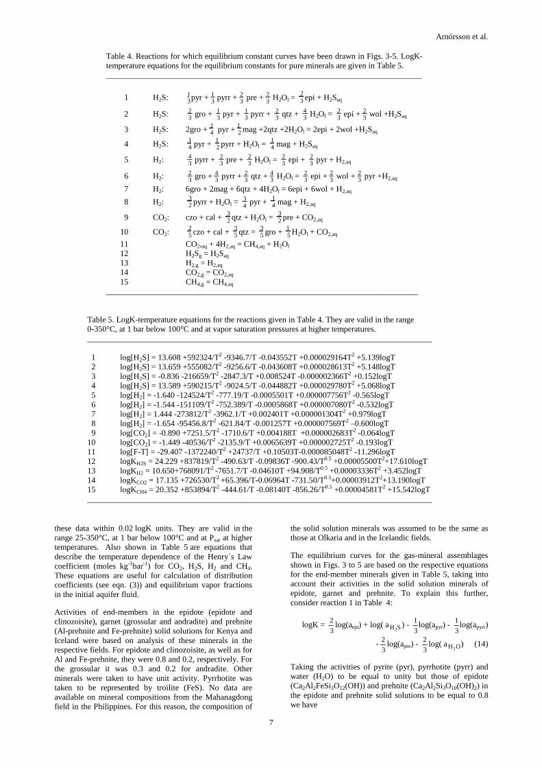
Table 4. Reactions for which equilibrium constant curves have been drawn in Figs. 3-5. LogK-temperature equations for the equilibrium constants for pure minerals are given in Table 5. _____________________________________________________________________________

1 H2S: 31pyr + 3

1 pyrr + 32 pre + 3

2 H2Ol = 23 epi + H2Saq

2 H2S: 32 gro + 3

1 pyr + 31 pyrr + 3

2 qtz + 34 H2Ol = 3

2 epi + 32 wol +H2Saq

3 H2S: 2gro + 14 pyr +

12 mag +2qtz +2H2Ol = 2epi + 2wol +H2Saq

4 H2S: 14 pyr +

12 pyrr + H2Ol =

14 mag + H2Saq

5 H2: 34 pyrr + 3

2 pre + 32 H2Ol = 3

2 epi + 32 pyr + H2,aq

6 H2: 32 gro + 3

4 pyrr + 32 qtz + 3

4 H2Ol = 32 epi + 3

2 wol + 32 pyr +H2,aq

7 H2: 6gro + 2mag + 6qtz + 4H2Ol = 6epi + 6wol + H2,aq

8 H2: 32 pyrr + H2Ol = 4

3 pyr + 14 mag + H2,aq

9 CO2: czo + cal + 32 qtz + H2Ol =

32 pre + CO2,aq

10 CO2: 25 czo + cal +

35 qtz =

35 gro +

15 H2Ol + CO2,aq

11 CO2,aq + 4H2,aq = CH4,aq + H2Ol 12 H2Sg = H2Saq 13 H2,g = H2,aq

14 CO2,g = CO2,aq

15 CH4,g = CH4,aq ____________________________________________________________________________

Table 5. LogK-temperature equations for the reactions given in Table 4. They are valid in the range 0-350°C, at 1 bar below 100°C and at vapor saturation pressures at higher temperatures. ____________________________________________________________________________________ 1 log[H2S] = 13.608 +592324/T2 -9346.7/T -0.043552T +0.000029164T2 +5.139logT 2 log[H2S] = 13.659 +555082/T2 -9256.6/T -0.043608T +0.000028613T2 +5.148logT 3 log[H2S] = -0.836 -216659/T2 -2847.3/T +0.008524T -0.000002366T2 +0.152logT 4 log[H2S] = 13.589 +590215/T2 -9024.5/T -0.044882T +0.000029780T2 +5.068logT 5 log[H2] = -1.640 -124524/T2 -777.19/T -0.0005501T +0.000007756T2 -0.565logT 6 log[H2] = -1.544 -151109/T2 -752.389/T -0.0005868T +0.000007080T2 -0.532logT 7 log[H2] = 1.444 -273812/T2 -3962.1/T +0.002401T +0.000001304T2 +0.979logT 8 log[H2] = -1.654 -95456.8/T2 -621.84/T -0.001257T +0.000007569T2 –0.600logT 9 log[CO2] = -0.890 +7251.5/T2 -1710.6/T +0.004188T +0.000002683T2 -0.064logT 10 log[CO2] = -1.449 -40536/T2 -2135.9/T +0.0065639T +0.000002725T2 -0.193logT 11 log[F-T] = -29.407 -1372240/T2 +24737/T +0.10503T-0.000085048T2 -11.296logT 12 logKH2S = 24.229 +837819/T2 -490.63/T -0.09836T -900.43/T0.5 +0.00005500T2+17.610logT 13 logKH2 = 10.650+768091/T2 -7651.7/T -0.04610T +94.908/T0.5 +0.00003336T2 +3.452logT 14 logKCO2 = 17.135 +726530/T2 +65.396/T-0.06964T -731.50/T0.5+0.00003912T2+13.190logT 15 logKCH4 = 20.352 +853894/T2 -444.61/T -0.08140T -856.26/T0.5 +0.00004581T2 +15.542logT ____________________________________________________________________________________

these data within 0.02 logK units. They are valid in the range 25-350°C, at 1 bar below 100°C and at Psat at higher temperatures. Also shown in Table 5 are equations that describe the temperature dependence of the Henry´s Law coefficient (moles kg-1bar-1) for CO2, H2S, H2 and CH4. These equations are useful for calculation of distribution coefficients (see eqn. (3)) and equilibrium vapor fractions in the initial aquifer fluid.

Activities of end-members in the epidote (epidote and clinozoisite), garnet (grossular and andradite) and prehnite (Al-prehnite and Fe-prehnite) solid solutions for Kenya and Iceland were based on analysis of these minerals in the respective fields. For epidote and clinozoisite, as well as for Al and Fe-prehnite, they were 0.8 and 0.2, respectively. For the grossular it was 0.3 and 0.2 for andradite. Other minerals were taken to have unit activity. Pyrrhotite was taken to be represented by troilite (FeS). No data are available on mineral compositions from the Mahanagdong field in the Philippines. For this reason, the composition of

the solid solution minerals was assumed to be the same as those at Olkaria and in the Icelandic fields.

The equilibrium curves for the gas-mineral assemblages shown in Figs. 3 to 5 are based on the respective equations for the end-member minerals given in Table 5, taking into account their activities in the solid solution minerals of epidote, garnet and prehnite. To explain this further, consider reaction 1 in Table 4:

logK = 2

3log(aepi) + log( aH2S ) -

1

3log(apyr) -

1

3log(apyrr)

-2

3log(apre) -

2

3log( aH2O) (14)

Taking the activities of pyrite (pyr), pyrrhotite (pyrr) and water (H2O) to be equal to unity but those of epidote (Ca2Al2FeSi3O12(OH)) and prehnite (Ca2Al2Si3O10(OH)2) in the epidote and prehnite solid solutions to be equal to 0.8 we have

Arnórsson et al.

8

log(aH2S

) = logK − 2

3log(0.8epi ) + 2

3log(0.8pre ) (15)

6. RESULTS

Assessment of the chemical evolution of hydrothermal fluids and of the extent to which they may have approached equilibrium according to certain chemical reactions is based on 1) the concept of local equilibrium within the larger open geothermal system, 2) data on the composition of well discharges, 3) modeling of aquifer fluid compositions and 4) thermodynamic data on gases, aqueous species and minerals.

The discharge of any well drilled into a volcanic geothermal system is expected to be composed of many fluid components that have travelled different distances at different velocites from their points of origin to the point of inflow into the well. The well may partly draw fluid from permeable fractures and partly from smaller pore spaces. The calculated composition of a single aquifer fluid with a specific composition and temperature, therefore, involves a simplification. This simplification is well approximated only if the well discharge is essentially derived from a single aquifer of a given temperature. In the present

contribution we have evaluated aquifer temperatures ( T f ) using downhole temperature measurements, circulation losses during drilling as well as the quartz and Na/K-geothermometers. The results are shown in Table 1.

The calculated composition of the initial aquifer fluid and the vapor fraction in this fluid are shown in Table 6 for the wells for which analyses are given in Table 1. They are based on model 3. The concentrations of H2S, H2 and CO2 in the initial aquifer fluid are depicted in Figs. 3 to 5.

A prominent feature of the diagrams of Figs. 3 to 5 is that the equilibrium constants for the two reactions involving CO2 are very similar for the selected mineral compositions in the temperature range of the aquifer fluids, 200-300°C (<0.28 logK units). This is also the case for two of the mineral assemblages that potentially could control H2S and H2, i.e. those which either include prehnite or magnetite in addition to the sulphide minerals (reactions nos. 1 and 4 for H2S and nos. 5 and 8 for H2, Tables 4 and 5). Equilibrium H2Saq and H2,aq concentrations for mineral assemblages that contain garnet are lower than for other assemblages, especially the one that also contains magnetite (Figs. 3-5) depending on the garnet and epidote compositions.

6.1 Hydrogen Sulphide and Hydrogen

For most of the wells in the Olkaria field in Kenya, the calculated aquifer fluid concentrations of H2S and H2 closely correspond to equilibrium with mineral assemblages 1 and 4, and 5 and 8, respectively (see Table 4). The equilibrium constants for each of these two pairs of mineral assemblages are very similar (Fig. 3). These results suggest that the aquifer vapor fraction is insignificant. Indeed the calculated vapor fraction value is most often around zero, the average being -0.03% by weight. Yet, some wells show low concentrations for these gases. These low concent-rations may be explained by steam loss amounting to a few percent, and therefore gas loss, from the boiling fluid flowing into these wells because the discharges are not only low in H2S and H2 but also in other gases. The steam loss from the flowing fluid is expected to occur in open sub-horizontal aquifers that convey fluid away from upflow zones.

Figure 3. Calculated concentrations of CO2, H2S and H2 in the total aquifer fluid of wells from the Olkaria field in Kenya. Red symbols represent the central part of the field, purple symbols the gas rich Olkaria West and green symbols the Domes Sector in the eastern part of the field. Dots denote excess enthalpy wells and crosses liquid enthalpy wells. The numbers by the curves refer to the reactions in Table 4.

In one of the Icelandic fields, Hellisheidi the picture is rather similar to that for Olkaria (Fig. 4). The average equi- librium vapor fraction is 0.2%, ranging fram -0.3% (degassed discharge) to 0.6%. For the two other Icelandic fields considered (Krafla and Nesjavellir), however, aquifer fluid concentrations of H2S and especially of H2 are higher than those at equilibrium with the mentioned mineral assemblages. The cause is considered to be the prescence of a relatively large initial vapor fraction in producing aquifers in these fields. If equilibrium is assumed to prevail according to reactions (1) and (5), the calculated aquifer fluid vapor fraction lies approximately in the range of 0-5% by weight. Two wells at Krafla have a very high aquifer fluid vapor fraction, 4 and 5.4%. They are drilled into a permeability anomaly of an explosive crater row. Both wells have a high discharge enthalpy, in particular the one with the higher equilibrium vapor fraction (2,649 kJ/kg). A third well has been drilled in this part of the area. It struck a zone of superheated vapor at ∼350°C. Possibly such vapor forms near the magma heat source and rises to the overlying liquid-dominated reservoir.

At Mahanagdong, the calculated aquifer fluid H2S and H2 concentrations are both considerably lower than those of Olkaria and in the Icelandic fields, and they show

Arnórsson et al.

9

considerable scatter, particularly for H2. In the case of H2S the data points scatter around the equilibrium values for the two garnet-bearing assemblages (reactions 2 and 3). In the case of H2, the data points scatter around the assemblage 7 (see Fig. 5). The results for Mahanagdong suggest that the garnet-magnetite mineral assemblage may control aqueous aquifer fluid H2S and H2 concentrations. These results are, however, only tentative as data on garnet and epidote distribution and composition at Mahanagdong are lacking. The large scatter of the H2 data points must, at least partly, be a reflection of the stoichiometry of the reaction involved (see Table 4). Aqueous H2 concentrations at equilibrium are very sensitive to garnet and epidote compositions.

6.2 Carbon Dioxide

The concentrations of CO2,aq in the aquifer fluid of all the study areas display a pattern that differs from those for H2S and H2. They can neither be explained by the presence of variable fractions of equilibrium vapor in the initial aquifer fluid nor by equilibration with hydrothermal minerals. The Mahanagdong aquifers have considerably higher CO2 concentrations than those in Iceland and those in all parts of the Olkaria area, except Olkaria West (Figs. 3-5).

The aquifer fluid CO2 concentrations at Olkaria are similar to, or higher than, those corresponding to equilibrium with the garnet-containing assemblage (Fig. 5). In the Icelandic field of Krafla, CO2 aquifer fluid concentrations are similar to those corresponding to equilibrium with the mineral assemblage that contains prehnite (reaction 9 in Table 4), or higher. During and shortly after the 1975-1984 volcanic episode at Krafla, CO2 well fluid concentrations used to be much higher than in the 2004 samples considered for the present study, and they rose, both in fumaroles and in wells, around the time when the first of nine small volcanic eruptions occurred in the area. This clearly demonstrates that the CO2 flux from the magma intruded into the roots of the geothermal system was too high for local equilibrium to be closely approached with hydrothermal mineral assemblages in the geothermal system. The decline of this flux with time has caused the CO2 aquifer fluid composition to come closer to equilibrium with hydrothermal mineral assemblages.

At Nesjavellir and Hellisheidi, calculated aquifer fluid CO2 concentrations are similar to or lower than those expected at equilibrium with the mineral assemblages considered. The cause of the low CO2 values is considered to be insufficient supply of this gas to the fluid to saturate it with calcite. When this is the case, the aquifer fluid CO2 concentration is externally controlled, i.e. by its flux into the geothermal fluid, either from a degassing magma or from the rock with which the geothermal fluid interacts, or both.

Aquifer fluids in the wellfield in the central part of the Olkaria area contain CO2 concentrations that closely match equilibrium with the two mineral assemblages depicted in Fig. 3 (reactions 9 and 10 in Table 4). By contrast, in the western part of the Olkaria area, around the volcano of Olkaria Hill, CO2 aquifer fluid concentrations are extremely high, and they also are high relative to equilibrium in the Domes Sector in the eastern part of the area. The cause is likely high flux of this gas from the magma heat source.

6.3 CO2-H2-CH4 gas equilibria

The activity product for the reaction

CO2,aq + 4H2,aq = CH4,aq + 2H2Ol (16)

has been calculated for all samples used for the present study and compared with the equilibrium constant for this reaction (Fig. 6). In Fig. 6A it was assumed that no equilibrium vapor was present in the initial aquifer fluid but Fig. 6B uses a vapor fraction for Olkaria and the Icelandic fields that was calculated from the H2S and H2 content of the well discharges. For the data from Mahanagdong, which show a large scatter for H2, it was not considered reliable to calculate an activity product for reaction (16) on the basis of an aquifer vapor fraction value calculated from the H2S and H2 content of the well discharges.

The Q and K values for Olkaria and the Icelandic fields, as calculated by taking into account the presence of equilibrium vapor, are remarkably constant at any temperature (Fig. 6B), which contrasts very much with the

Figure 4. Calculated concentrations of CO2, H2S and H2 in the total aquifer fluid of wells from the Krafla (red), Nesjavellir (purple) and Hellisheidi (green) fields in Iceland. Dots denote excess enthalpy wells and crosses liquid enthalpy wells. The numbers by the curves refer to the reactions in Table 4.

larger scatter for the total aquifer fluid (no equilibrium vapor present). The results in Fig. 6B suggest that equilibrium is closely approached when temperatures reach about 300°C but at lower temperature formation of CH4 or loss of CO2 or H2 from solution is required to bring the fluids to equilibrium.

7. CONCLUSIONS

Excess discharge enthalpy of wet-steam wells in the volcanic geothermal fields of Olkaria (Kenya), Mahanagdong (Philippines), Krafla, Nesjavellir and Hellis-heidi (Iceland) is dominantly produced by segregation of vapor and liquid flowing through the depressurization zone around the wells, as deduced from the gas composition of their discharges. The reason is considered to be retention of some of the liquid in the aquifer due to its adsorption onto

Arnórsson et al.

10

mineral grain surfaces by capillary forces. The concentrations of H2S in the initial aquifer liquid at Olkaria and in the Icelandic fields are controlled by close approach to equilibrium with hydrothermal mineral assemblage 1 or 4 whereas reactions 5 or 8 seem to control aqueous aquifer liquid H2 concentrations (Table 4). At Mahanagdong the concentrations of H2S and H2 in the initial aquifer fluid are probably controlled by the garnet-magnetite bearing mineral assemblage (reactions 3 and 7 in Table 4). The concentrations of CO2 are equilibrium controlled at Olkaria but by its supply to the geothermal fluid in the other areas. Equilibrium vapor fraction is small in the Olkaria and

Hellisheidi fields, 0.03% and 0.5% by weight on average, respectively. By contrast, they are relatively high at Krafla and Nesjavelllir, 1.2% and 0.9% by weight on average. This excludes two Krafla wells, which have almost 5% and 10% initial aquifer vapor by weight. The aquifer fluid for these two wells is vapor-dominated in terms of fluid volume. The large scatter of the H2 data from Mahanagdong makes estimation of the vapor fraction in producing aquifers unreliable. Gas-gas equilibrium for the Fischer-Tropsch reaction is closely approached at 300°C but departure from equilibrium increases with decreasing temperature.

Table 6. Calculated composition of the initial aquifer fluid producing into selected wet-steam wells. The primary data are given in Table 1. Concentrations are in mg/kg.

1 2 3c 4 5 6 7

h f ,t 1067 1142 1071 1451 1334 1173 1309

T f 242 262 247 299 291 267 286

Pe 10.0 10.0 50.1 46.2 36.2 43.9

T e 180 180 264 259 245 256

X f ,v % 0.03 -0.16 0.13 2.5 2.6 0.19 2.7

V f ,t 3.7 2.3 1.5 5.2 1.3 1.5

V e,l 2.7 1.3 0.05 4.2 0.3 0.5

pH 6.97 6.25 7.11 7.25 7.68 7.28 5.38 SiO2 407 563 485 648 609 522 574 B 4.2 4.5 0.59 1.21 1.22 0.97 47.0 Na 372 844 206 176 110 159.2 1941 K 58.7 136 30.0 40.3 24.3 25.9 393 Ca 0.39 0.44 2.31 1.16 0.23 0.28 28.9 Mg 0.007 0.046 0.004 0.0010 0.0050 0.009 0.026 Al 0.56 0.44 1.35 1.25 1.27 1.38 0.234 Fe 0.014 0.013 0.012 0.0017 0.0008 0.0087 0.068 CO2

a 384 43,026 319.6 519.2 708.9 162.9 4615 H2S

b 37.4 30.8 56.1 171.5 270.4 162.6 47.5 SO4 38.2 73.7 228.3 125.2 1.5 6.0 16.9 Cl 465 158.0 43.1 110.0 85.6 157.6 3346 F 40.3 69.1 0.91 1.03 0.90 0.87 1.20 H2 1.02 0.46 1.80 6.65 8.79 2.83 0.31 CH4 1.03 2.94 1.07 0.10 0.69 0.43 3.03 N2 11.35 69.4 34.5 7.36 13.26 9.98 13.2

h f ,t : Aquifer fluid enthalpy (kJ/kg). T f : Aquifer temperature (°C). Pe : Vapor segregation pressure (bar abs.). T e :

Phase segregation temperature (°C). X f ,v : Initial aquifer fluid vapor fraction. V f ,t : Relative mass (to well discharge)

of initial aquifer fluid. V e,l : Relative mass (to well discharge) of boiled (and degassed) water retained in aquifer. aTotal

carbonate carbon as CO2. bTotal sulphide sulphur as H2S. cLiquid enthalpy well. Therefore values for Pe , T e , V f ,t

and V e,l are not reported. 1: Olkaria 15, 2: Olkaria 301, 3: Krafla 27, 4: Krafla 32, 5: Nesjavellir 21, 6: Hellisheidi 7, 7: Mahanagdong 16D. Numbers after local name indicate well number.

REFERENCES

Ármannsson, H.: CO2 emission from geothermal plants. Proceedings, International Conference on Multiple Integrated Uses of Geothermal Resources, Reykjavík, Iceland, (2003), 56-62.

Ármannsson, H., Gíslason, G. and Hauksson, T.: Magmatic gases in well fluids aid the mapping of flow pattern in a geothermal system. Geochim. Cosmochim. Acta, 46 (1982), 167-177.

Arnórsson, S., Björnsson, S., Muna, Z.W. and Ojiambo, S.B.: The use of gas chemistry to evaluate boiling processes and initial steam fractions in geothermal reservoirs with an example from the Olkaria field, Kenya. Geothermics, 19 (1990), 497-514.

Arnórsson, S., Stefánsson, A. and Bjarnason, J.Ö.: Fluid-fluid interaction in geothermal systems. Reviews in Mineralogy & Geochemistry, 65 (2007), 259-312.

Bödvarsson, G.: (1961) Physical characteristics of natural heat resources in Iceland. Jökull, 11 (1961), 29-38.

D´Amore, F. and Panichi, C.: Evaluation of deep temperatures in hydrothermal systems by a new gas geothermometer. Geochim. Cosmochim. Acta, 44 (1980), 309-332.

D´Amore, F. and Truesdell, A.H.: Calculation of geothermal reservoir temperatures and steam fractions from gas compositions. Trans. Geotherm. Res. Council, 9 (1985),

305-310. Fernandez-Prini, R., Alvarez, J.L. and Harvey, A.H.: (2003)

Henry´s constants and vapor-liquid distribution

Arnórsson et al.

11

constants for gaseous solutes in H2O and D2O at high temperatures. J. Phys. Chem. Ref. Data, 32 (2003), 903-916.

Giggenbach, W.F.: Geothermal gas equilibria. Geochim. Cosmochim. Acta, 44 (1980), 2021-2032.

Goff, F. and Janik, C.J.: Geothermal systems. Encyclopedia of Volcanoes. Sigurdsson, H. (ed.) Pergamon Press, New York, (2000), 817-834.

Gudmundsson, B.T. and Arnórsson, S.: Geochemical monitoring of the Krafla and Námafjall geothermal areas, N- Iceland. Geothermics, 31 (2002), 195-243.

Gudmundsson, B.T. and Arnórsson, S.: Secondary mineral-fluid equilibria in the Krafla and Námafjall geothermal systems, Iceland. Appl. Geochem., 20 (2005), 1607-1625.

Herras, E.B., Licup, A.C., Vicedo, R.O., Parilla, E.V. and Jordan, O.T.: The hydrological model of the Mahanagdong geothermal system. GRC Transactions, 20, (1996), 681-688.

Figure 5. Calculated concentrations of CO2, H2S and H2 in the total aquifer fluid of wells from the Mahanagdong fields in the Philippines. Dots denote excess enthalpy wells and crosses liquid enthalpy wells. The numbers by the curves refer to the equations in Tables 4 and 5.

Holland, T.J.B. and Powell, R.: (1998) An internally consistent thermodynamic dataset for phases of petrological interest. J. metamorphic Geol., 16, (1998), 309-343.

Kissling, W.M., Brown, L.K., O´Sullivan, M.J., White, S.P. and Bullivant, D.P.: Modelling chloride and CO2 chemistry in the Wairakei geothermal reservoir.

Geothermics, 25 (1996), 285-305. Reyes, A.G., Giggenbach, W.F., Saleras, J.R.M., Salonga,

N.D. and Vergara, M.C.: Petrology and geochemistry of Alto Peak, a vapor-cored hydrothermal system, Leyte province, Philippines. Geothermics, 22 (1993), 479-519.

Robie, R.A. and Hemingway, B.S.: Thermodynamic properties of minerals and related substances at 298.15 K and 1 bar (105 Pascals) pressures and at higher temperatures. U.S. Geol. Surv. Bull., 2131 (1995).

Stefánsson, A. and Arnórsson, S.: Gas pressures and redox reactions in geothermal fluids in Iceland. Chem Geol., 190 (2002), 251-271.

Figure 6. Calculated activity products for the Fischer-Tropsch reaction assuming (A) no vapor fraction in the aquifer fluid and (B) vapor fraction calculated using eqn. (5). The curves represent the equilibrium constant expressed in terms of aqueous gas concentrations. Black, red, green, blue and purple symbols represent Mahanagdong, Nesjavellir, Hellisheidi, Krafla and Olkaria, respectively.

APPENDIX 1 – DERIVATION OF EQUATIONS FOR MODEL 6: OPEN SYSTEM; STEAM OUTFLOW

In this model, there is no conductive heat flow from the surroundings, and no liquid is retained in the formation.

Thus, Q e= 0 and M e,l = 0. Some vapor is assumed to be

lost from the fluid flowing into the well so M e,v ≠ 0. The conservation equations for water mass, water enthalpy and mole number of chemical components are thus:

M d ,t = M f ,t − M e,v (1A)

h d ,t M d ,t = h f ,t M f ,t − he,vM e,v (2A)

msd ,t M d ,t = ms

f ,t M f ,t − mse,vM e,v (3A)

mrd ,t M d ,t = mr

f ,t M f ,t (4A)

Arnórsson et al.

12

where s refers to a gaseous species and r denotes a non-volatile component. Inserting eqn. (1A) into (2A) and

eliminating M e,v gives

M f ,t

M d ,t=

h d ,t − h e,v

h f ,t − h e,v (5A)

Similarly, solution of eqns. (1A) and (3A) yields

M f ,t

M d ,t=

msd ,t − ms

e,v

msf ,t − ms

e,v (6A)

The equation below relates the concentration of gas s in the

total fluid in the intermediate zone ( mse,t ) at temperature T e

to its concentration in the vapor and liquid water phases:

mse,t = ms

e,l (1− X e,v ) + mse,v X e,v (7A)

The coefficient describing the distribution of gas s between the liquid and vapor phases is given by

Dse ≅

mse,v

mse,l

≅55.51

Ptot Ks (8A)

(see Arnórsson et al., 2007). Inserting eqn. (8A) into (7A) by

eliminating mse,l yields

mse,t = ms

e,v X e,v 1−1

Dse

⎛

⎝ ⎜ ⎜

⎞

⎠ ⎟ ⎟ +

1

Dse

⎡

⎣ ⎢ ⎢

⎤

⎦ ⎥ ⎥ (9A)

and X e,v is given by

X e,v =h f ,t − h e,l

h e,v − h e,l (10A)

Just before vapor is lost from the flowing fluid in the

intermediate zone at T e , the concentration of gas s is the

same in the initial aquifer fluid ( msf ,t ) and the total fluid in

the intermediate zone ( mse,t ), i.e. ms

e,t = msf ,t . Thus, eqn.

(9A) can be expressed as

mse,v = ms

f ,t X e,v 1−1

Dse

⎛

⎝ ⎜ ⎜

⎞

⎠ ⎟ ⎟ +

1

Dse

⎡

⎣ ⎢ ⎢

⎤

⎦ ⎥ ⎥

−1

(11A)

Once the temperature of phase segregation in the inter-

mediate zone ( T e ) has been selected, all variables in eqns.

(10A) and (11A) are known, except h f ,t , msf ,t and ms

e,v .

By equating the right hand sides of eqns. (5A) and (6A) and rearranging we find that

h f ,t =ms

f ,t − mse,v

msd ,t − ms

e,v

⎛

⎝ ⎜ ⎜

⎞

⎠ ⎟ ⎟ ⋅ (h d ,t − h e,v ) + h e,v (12A)

If it is assumed that the concentration of a gas (H2S or H2) in

the initial aquifer liquid water ( msf ,l ) is known (fixed by a

temperature-dependent equilibrium with a hydrothermal

mineral assemblage), msf ,t can be expressed as (see eqn.

(2))

msf ,t = ms

f ,l X f ,v Dsf −1( )+1[ ] (13A)

Equations (11A), (12A) and (13A) may now be solved

iteratively. We first estimate a value for h f ,t to get X f ,v

and X e,v from eqns. (1) and (10A), respectively. Then msf ,t

is obtained from (13A). With this value, mse,v is found from

eqn. (11A). These results are substituted into eqn. (12A) to

obtain a new value for h f ,t . The procedure is repeated until

a consistent value for h f ,t is obtained. At this point X f ,v

and X e,v are known, as is the concentration of the gas under consideration (H2S or H2) in the total fluid in the feed zone

( msf ,t ) and in the vapor phase in the intermediate zone

( mse,v ). Now ms

e,l may be obtained from eqn. (7A) for this

gas since mse,t = ms

f ,t , and msf ,v may be found from an

equation analogous to (7A) for the feed zone, since msf ,l is

assumed fixed by equilibrium and thus known. Finally,

M f ,t may be obtained from eqn. (5A) since M d ,t and h d ,t are measured quantities.

For gases other than the one above, we proceed as follows:

Equation (11A) is solved for msf ,t , which is substituted into

eqn. (6A). The resulting equation is then solved for mse,v to

give

mse,v = ms

d ,t ⋅ V f ,t (1− X e,v ) ⋅1

Dse

−1⎛

⎝ ⎜ ⎜

⎞

⎠ ⎟ ⎟ +1

⎡

⎣ ⎢ ⎢

⎤

⎦ ⎥ ⎥

−1

(14A)

where V f ,t = M f ,t /M d ,t . Now mse,v may be computed

directly from (14A), and a value for msf ,t is then found from

(11A). Since mse,t = ms

f ,t , we can find mse,l from eqn (7A).

Finally, msf ,l can be obtained from eqn. (13A) and then

msf ,v from a feed-zone analogue of eqn. (7A). Alternatively

and equivalently, msf ,v could be found by substituting ms

e,v

from eqn. (14A) into (11A) and then eliminating msf ,t

between this new equation and a feed-zone analogue of (9A). This approach yields

msf ,v = ms

d ,t ⋅ X e,v (1−1

Dse

) +1

Dse

⎡

⎣ ⎢ ⎢

⎤

⎦ ⎥ ⎥ ⋅ X f ,v (1−

1

Dsf

) +1

Dsf

⎡

⎣ ⎢ ⎢

⎤

⎦ ⎥ ⎥

−1

⋅ V f ,t (1− X e,v ) ⋅1

Dse

−1⎛

⎝ ⎜ ⎜

⎞

⎠ ⎟ ⎟ +1

⎡

⎣ ⎢ ⎢

⎤

⎦ ⎥ ⎥

−1

(15A)

The feed-zone analogue of (9A) would then give msf ,t , and

so on.

The concentration of a non-volatile component r in the initial aquifer fluid can be obtained from

mrf ,t = mr

f ,l (1− X f ,v ) (16A)

and eqn. (4A), which yields

mrf ,l = mr

d ,t V f ,t (1− X f ,v )[ ]−1 (17A)

where V f ,t is equal to M f ,t /M d ,t as before.