Embed Size (px)
Citation preview

Garrison, 2015 Technical Report
Estimated Injury of Sea Turtles in Neritic Habitats Associated with Exposure to DWH Oil
Lance P. Garrison
DRAET: 31 August 2015
1. SUMMARY
During the Deepwater Horizon (DWH) oil spill in 2010, surface oil covered more than 100,000 km^ of
surface waters from offshore areas across the continental shelf and into nearshore areas (DWH Trustees,
2015, Section 4.2). The Trustees performed several surveys to document the presence o f natural resources,
such as sea turtles, within the DWH footprint, as well as potential exposures and injuries to these resources
caused by DHW (DWH Trustees, 2015). In this study, total abundance, potential exposures, and estimated
injuries to sea turtles occupying continental shelf waters and nearshore coastal waters (i.e., “neritic”
habitats) were quantified by combining data and analyses from linc-transcct aerial sun^eys, satellite
telemetry studies, and analyses o f the temporal and spatial overlap of individual turtles with surface oil.
These estimates were combined with mortality estimates based on observed degree of oiling on turtles
rescued during 2010 to quantify total injuries to sea turtles in nentic habitats.
2. INTRODUCTION
Five species o f sea turtles inhabit the G ulf o f Mexico (GoM): loggerheads (Caretta caretta), Kemp’s
ridleys {Lepidochelys kempii), green turtles (Chelonia mydas), hawksbills {Eretmochelys imbricata), and
leatherbacks {Dermochelys coriacea). Loggerheads, Kemp’s ridleys, green turtles, and hawksbills are in
the Cheloniidae family (hard shells), and leatherbacks are in the Dermochelyidae family. Loggerheads are
listed as “Threatened” under the Endangered Species Act (ESA), while the other four species are listed as
“Endangered” under the ESA. Sea turtles in the northern GoM face multiple anthropogenic threats
presently, and all populations are depleted relative to historical levels (Wallace et ah, 2011).
After spending years in an open-ocean or oceanic phase, juvenile sea turtles recmit into continental shelf or
neritic areas, where they continue growing to larger sizes over several additional j^ears - or even decades
(Bolten, 2003). Turtles reach adulthood and mostly remain in continental shelf areas for the rest o f their
lives (Bolten, 2003). The DWH oil spill overlapped with vital marine habitats for sea turtles, including
continental shelf and nearshore areas occupied by neritic juveniles and adnlts (Wallace et ah, 2015).
Consequently, the Tmstees conducted aerial surveys throughout the northern GoM on the continental shelf
and in nearshrore areas to count neritic turtles at the surface. These surveys were designed to allow for
calculation o f estimates of turtle abundance across the survey area through the study period, and
DWH-AR0149505

Garrison, 2015 Technical Report
subsequently for calculation o f overall abundances. These estimates were then used in injury quantification
(DWH Tmstees, 2015, Section 4.8).
3. METHODS
3.1 DESCRIPTION OF APPROACH
Line-transect aerial survey data were were analyzed using “Distance” analysis (Buckland et al., 2001,
Laake and Borchers, 2004) to estimate the abundance o f turtles within the surveyed area and to derive
spatially explicit maps o f turtle density. Double-observer methods (Laake and Borchers, 2004) were used
during broadscale surveys conducted during 2011-2012 to estimate the probahility of detection on the
trackline and therefore correct abundance estimates for the likelihood that a turtle at the surface was
detected by the survey teams (i.e., “perception bias”). These data were combined with estimates of the
probability o f individual turtles becoming “heavily oiled” based on statistical relationships between
observed oiling status o f rescued turtles and spatio-temporal proximity to satellite-derived surface oil data
(Wallace et al., 2015). Based on information gathered during rescue operations, physical fouling in surface
oil was determined to be the primary route of exposure and adverse effects on sea turtles (Stacy, 2012;
Wallace et al., 2015). Moreover, these adverse effects of direct contact with oil were expected to increase
with the degree o f oiling observed. Therefore, the outcome o f this analysis is an estimate o f the total number
o f “heavily oiled” neritic turtles based on estimated degree o f exposure to DWH surface oil.
The equation used to estimate the total number o f turtles injured (by taxon) is given by:
(1) n in ju red = £f= i pa^p(o)- ,
and,
(2) N I ^ r e d = A -^ ^ ^ ^ ^
where:
n = number o f turtle “groups” sighted during aerial surveys
Si = size o f group i (equal to 1 for individual turtles)
pdi = probability of detection conditional on the animal being at the surface (Distance analysis estimate)
p(0)i = detection probability on trackline (Estimated from Mark-Recapture Distance Sampling [MRDS]
analysis)
DWH-AR0149506

Garrison, 2015 Technical Report
A = total extrapolation area
L = total trackline surveyed during aerial survey
w = tnincation distance (1/2 strip width)
ninjured = estimatcd number of injured turtles within the surveyed area
Ninjured = total estimated number o f injured turtles (extrapolated population)
pHeavilyOiledi = probability that observed turtle is heavily oiled based on logistic regression output in
Wallace et al. (2015)
The probability o f “heavy oiling” (pHeavilyOiled) is derived from a logistic regression model that
estimated the probability that a captured turtle was “heavily oiled” based on the statistical relationship
between observed turtle oiling status and the satellite-derived surface oil environment [i.e., oil measured by
synthetic aperture radar (SAR; Garcia-Pineda et al., 2009; Graettinger et a l , 2015)] in the area around and
time before turtle captures (Wallace et al., 2015). The model may be interpreted as an assessment o f the
probability o f intersecting sufficient surface oil in order to become “heavily” oiled. However, this model
was developed using data from small surface-pelagic turtles that spend nearly 100% of their time near the
surface (Bolten, 2003). In contrast, larger, neritic turtles spend less time at the surface (Bolten, 2003), and
therefore should have a lower probability o f intersecting surface oil compared to surface-pelagic turtles.
Nonetheless, all sea turtles—whether small, oceanic juveniles, or large neritic juveniles or adults— must
spend time at the surface to breathe, rest, bask, and feed, and these fundamental behaviors put turtles at
continuous and repeated risk o f exposure anywhere that the ocean surface was contaminated by DWH oil
(Wallace et al. 2015).
The parameter pdj (equation 1) is an estimate o f the probability that an animal is detected by the
survey team conditional on it being at the surface. The estimated detection on the trackline {g(O)i) is an
estimate o f “perception bias”, the probability o f detection on the trackline conditional on the animal being
available for detection by both teams. An estimate of the prohabilty o f an animal being at the surface is
available from tag-telemetry studies (see below). However, this probability was excluded from equation 1
to account for the reduced probahility o f a neretic turtle being at the surface (and thus intersecting with
surface oil) compared to pelagic turtles.
The resulting injury (mortalities) for turtles in neretic habitats from this analysis are shown in
Table 1. It should be noted that this includes only turtles larger than approximately 40 cm in length because
smaller turtles cannot be detected reliably from the aircraft (Schroeder 1985).
DWH-AR0149507

Garrison, 2015 Technical Report
3.2 FIELD METHODS AND DATA SOURCES
Aerial Survey Methods
A DeHavilland DHC-6 Twin Otter was used to conduct aerial surveys, and transects were flown at
an altitude o f 182 m and an airspeed o f 185 kin/lir. The aircraft position was recorded at 10 second intervals
using a GPS, and environmental parameters were recorded including weather conditions (e.g, clear, fog,
rain), visibility, water color, water turbidity, sea state, and glare. Sun^eys were typically flown during
favorable sighting conditions at Beaufort sea states less than or equal to 4 (surface winds <12 knots).
Visual observers searched for marine mammals and sea turtles from directly beneath the aircraft
out to a perpendicular distance o f approximately 600m from the trackline. Due to the configuration o f the
observing bubble windows and the position o f the helly window obsen^er, the trackline directly under the
airplane could be reliably surveyed. When the observed sea turtle or marine mammal was perpendicular to
the aircraft, the observer measured the angle from the vertical to the animal (or group) using a digital
inclinometer or estimated the angle based upon markings on the windows indicating 10-degree inter\'als.
This sighting angle, 0, was converted to the perpendicnlar distance from the trackline (PSD) by PSD =
tan(0) X Altitude. For some marine mammal sightings, the aircraft circled at lower altitude for species
identification and group size estimation. Sea turtles were identified to species visually by the observer
based upon size, shell shape, shell coloration, and the relative size o f the head to the body. If a reliable
species identification could not be made, then the turtle was recorded as an “unidentified hardshell turtle,”
which included species in the Family Chelonidaee (e.g., loggerheads, Kemp’s ridleys, green turtles).
Leatherback turtles, the sole extant member o f the Family Dermochelyidae, were not mistakable.
During the 2010 synoptic surveys, a single observer team was used including two observers
stationed in bubble windows on both sides in the forward portion of the aircraft, a helly window obserx^er,
and a data recorder. During the 2011-2012 broadscale surveys, a two-team configuration was used that
allowed estimation o f perception bias. In this case, the forward team consisted of observers stationed in
bubble windows on either side of the aircraft. The aft team consisted o f a belly window observer and an
observer stationed at a large bubble window on the right side of the aircraft. Both teams had independent
data recorders and did not communicate with each other while actively sur\'eying. All turtle sightings were
recorded independently and then evaluated after the survey to determine if each sighting was observed by
both teams based upon the time and location o f the observation. During the summer 2011 survey, a different
aircraft was used that did not have the downward looking aft belly window. Hence, the aft team during that
survey consisted only o f a recorder and an observer looking out o f a large bubble window on the right side
o f the aircraft.
Survey Design - 2010 Synoptic Surveys
DWH-AR0149508

Garrison, 2015 Technical Report
Aerial line-transect surveys were conducted between 28 April and 2 September 2010 in the
north-central Gulf o f Mexico ranging between 91.4°W and 86.8°W longitude covering the southern and
eastern coasts o f Louisiana, Mississippi Sound, Alabama, and a portion o f the westem Florida panhandle
(Figure 1). The surveys included primarily waters from the shoreline to the 200 m isobaths with limited
survey effort in waters between 400-2000 m bottom depth. Analyses for this study are limited to waters
<200m in depth. Sun'ey tracklines were spaced at regular intervals (-20 km apart) and were oriented
perpendicular to the shoreline and bathymetry gradients. Survey tracklines covering the entire area were
designed to be conducted in 3 to 4 flight days. However, weather conditions typically increased the length
o f this window, or in some cases, prevented the completion of an entire survey. The tracklines were covered
during seven sampling periods that ranged between 2 and 7 days in length (Table 2). These survey periods
were intended to be spaced approximately 10 days apart; however, this could not always be achieved due to
weather conditions or logistical issues.
Survey Design - 2011-2012 Broadscale Surveys
The 2011-2012 broadscale surveys covered waters over the continental shelf from Brownsville, TX
(U.S./Mexico border) to north o f the Dry Tortugas (Figure 2). Tracklines were oriented perpendicular to the
shoreline and bathymetry gradient and spaced 15 km apart throughout most o f the survey. Survey tracklines
followed uniform spacing from a random start point and were divided into strata to accommodate changes
in the orientation of the coastline. The survey as planned encompassed approximately 16,000 km o f survey
effort which was covered during -60-day flight windows during the spring (13 April-31 May, 2011),
summer (11 July - 4 September, 2011), fall (12 October - 4 December, 2011) and winter (13 January - 9
March, 2012). Due to weather conditions, not all planned tracklines were covered during each survey
(Table 3). In addition to tracklines over the continental shelf, “zig-zag” tracklines were flown to cover
deeper waters along the shelf break. However, data from these tracklines are not included in the current
analysis.
Satellite Telemetry TagMethods
The amount o f time turtles spend near the surface is critical for developing corrections for
availability to the survey team given that turtles spend a significant amount o f time underwater. Thus,
researchers deployed Wildlife computers MK-lOA telemetry tags on adult and sub-adult Kemp’s ridley and
loggerhead sea turtles in the Gulf o f Mexico during 2011 and 2012. to provide information on movement
patterns and dive-surface behavior. A total of 22 Kemp’s Ridley turtles and 30 loggerhead turtles were
included in the current analysis (Table 4). This included both in-water captures (i.e. captures by trawling) of
sub-adults and turtles encountered on nesting beaches (Table 4, Figure 3). Twenty o f tliese tags (10 Kemp’s
DWH-AR0149509

Garrison, 2015 Technical Report
ridley, 10 loggerheads) were deployed on nesting females by researchers from the U.S. Geological Survey
(USGS), Department of Interior under NRDA projects. The remaining tags were deployed under an
interagency agreement between NMFS-SEFSC and the Beureau o f Offshore Energy Management (SEFSC,
unpublished data).The MK-lOA tags report both ARGOS and GPS dervied location data and report
summaries of dive behaviors as histograms show'ing the amount o f time spent in designated depth “bins”
during a given reporting period. For this effort, the tags reported depth summaries in four-hour intervals
which allowed evaluation o f potential diurnal changes in dive-behaviors. The first depth bin was defined as
0-2 m below the surface, as it was assumed that turtles are visible to the aerial survey near the surface and
slightlybeneath the surface. Hence, during each reporting interval, the precentage o f time the turtle spent in
the first reporting bin w'as assumed to be equivalent to the percentage o f time that the turtle is available to
the sun^ey. This metric was incorporated into the abundance estimation as described below.
Habitat Data
Spatially explicit habitat models were derived to examine spatial distribution and density o f sea
turtles at weekly intervals during the DWH oil spill. The synoptic aerial survey data collected during 2010
were used to derive these models, which included bottom depth, sea surface temperature, and chlorophyll a
concentration as explanatory variables. Bathymetry data for the continental shelf was obtained from the
ETOPO-1 global digital elevation model which provides a 1-arc minute resolution grid o f bottom depth
(Amante et ah, 2009).
Sea surface temperature (SST) and surface chlorophyll-a (CHE) were obtained from the NASA
Ocean Color MODIS platform (http://oceancolor.gsfc.nasa.gov/). Eight-day composites o f SST and CHE
were obtained from the level-3 products distributed from the Ocean Color website. These images are
available as masked and georeferenced HDF files with global coverage. The downloaded images w'ere
parsed to the desired spatial coverage, and cells close to land or obscured by clouds were masked in the
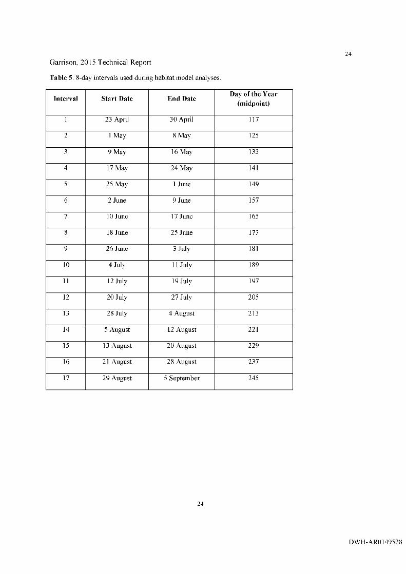
available imagery. Imagery used in this analysis was from 17, 8-day periods with the first period starting on
23 April 2010 (Table 5).
3 .3 ANAEYTICAL METHODS
Data were anayzed within the framework o f line transect distance analysis with incomplete
detection on the trackline (see Buckland et al. 2001 and Laake and Borchers, 2004 for review). Briefly, in
addition to collecting information on the location and occurrence o f animals along survey tracklines, the
perpendicular sighting distance (PSD) is measured as described above. The distribution o f the number of
sightings as a function of PSD [i.e., the sighting function oxg(x) where x is the PSD] can be used to estimate
the probability of detection o f objects within the surveyed area. Standard distanec analysis assumes that
DWH-AR0149510

Garrison, 2015 Technical Report
detection probability on the trackline [g(0)} is equal to 1. In the case o f sea turtles, detection on the trackline
is incomplete (< 1) because some animals at the surface may be missed by the observ er and/or some
animals may be beneath the surface and hence not available to be detected by the survey. Thus, an unbiased
estimate o f the number o f animals within the sun^eyed area is calculated as:
(3) Uc = paipdip(0)i ’
where n is the number o f detected animal groups (sightings), 5 is the size o f the group (number o f animals in
the group), pa is the probability that the group is available to the survey, p d is the probability o f detection
within the surveyed strip, and p(0) is the probability o f detection on the trackline for the group.
The abundance o f animals within the entire surveyed area is thus calculated as:
where L is the total length (km) o f trackline surveyed, w is the “truncation’' distance [i.e., the maximum
PSD (km) from the line at which sightings are recorded or included in the analysis], andri is the area (km^)
o f the region over which the estimation o f abundance is desired. Parameters to be estimated therefore
include pa ,pd , andp(0) for each turtle sighting.
Estimation o f availability (pa)
For each turtle group observed during the aerial survey, the probability o f availability (pa in
equation 3) was calculated as a stratified mean proportion of time spent on the surface as a function of
species, season, and water depth. This mean was calculated from the summarized telemetiy^ data for each
species. The proportion of time spent at depth < 2 m was reported in four-hour periods from each tag. These
values are therefore nested within each turtle, as it is expected that there is dependence between the four
hour periods within each turtle. Since all four hour periods are not reported due to variation in the
opportunity for transmission of satellite data, this becomes equivalent to a two-stage cluster sampling of
dive behaviors for calculating associated means and variances. Tag position data from both GPS and
ARGOS locations were filtered to remove erroneous locations (e.g., on land) or highly uncertain positions
from the ARGOS data quality flags reported with each location. The best (i.e., most reliable, highest
quality) position for each day was retained. Locations oustide of the range of the aerial surveys inside
estuarine waters or in deep waters were also filetered out o f this analysis. The bottom depth o f each best
daily location was derived from the ETOPO1 digital elevation model, whch was used as the depth value for
all dive data reported for that day. Based upon preliminary analyses o f the depth distribution o f turtle tag
DWH-AR0149511

Garrison, 2015 Technical Report
position, tag locations were divided into “shallow” (<25 m depth) and “deep” (>= 25m depth) locations to
reflect potential dive behavior changes as a function o f bathymetry. Dive behavior data was also split into
“Day” (0600-1800 local time) and “Night” (1800-0600 local time) based upon the time interval of the depth
summary. Finally, data were categorized into four seasons: Winter (Dec-Feb), Spring (Mar-May), Summer
(Jun-Aug), and Fall (Sep-Nov). These factors (Depth, Day/Night, Region, and Season) were included as
fixed factors in a Generalized Linear Mixed Model (GLMM) ANOVA with the individual turtle as a
random effect to evaluate effects on dive-surface behavior (proc GLMMIX, SAS v9.2). Following the
selection of significant factors, mean (and variances) of the proportion o f time spent at the surface were
used as estimates o f pa for each turtle sighting as a function if its location and season o f observation.
Estimation o f detection probability on the trackline [p(0)]
Detection probability on the trackline \p(0)} was estimated using the independent-observer
approach described in Laake and Borchers (2004) and using the MRDS package in R (Laake et al. 2015).
The high speed o f the aircraft and the resulting short viewing inten^al for each turtle means that turtle
sightings are essentially instantaneously available to both teams at the same time. Th\xs,p(0) in this case is
an estimate o f the likelihood o f at least one team on the survey detecting the turtle conditional on its being at
the surface at the time the aircraft passed over its location. Two independent survey teams were deployed
only during the 2011-2012 broadscale surveys, thus data collected from these surveys were used to model
and estimate p(0) for the 2010 synoptic surveys. The forward survey team during the 2011-2012 surv^eys
had the same viewing position and configuration as the team during the 2010 surveys. Hence, the relvant
variable to be modelled is Tp(0) for the forward survey team.
As noted above, the aft survey team had limited visibility on the left side o f the aircraft. Thus,
turtles occurring at sighting angles more than 30 degrees from vertical on the left side were not available to
the aft team, and were therefore removed from the analysis o f p(0). A single model was derived across all
four surveys conducted during 2011-2012 in order to better accoimt for variability across different survey
teams. The aircraft configuration during the summer 2011 survey did not include the belly window;
however, inspection o f the data indicated that the trackline was effectively surveyed hy the bubble window
observer, therefore this survey was also included in the analysis. However, sightings on the left side o f the
aircraft greater than 10 degrees away from the vertical were excluded for the summer survey as they were
not available to the aft team.
For each turtle sighting that was available to hoth teams, it was determined from the sighting record
whether it was seen by the forward team only, the aft team only, or by both teams. Using the MRDS
package in R these data were modelled to derive estimates o f p(0) as a function o f sea state (Beaufort
scale), glare, and obsen^er (forward vs. aft) team using the “full independence” independent observer model
DWH-AR0149512

Garrison, 2015 Technical Report
(Laake and Borchers, 2004). Additional sighting condition variables (water color, turbidity, and light
conditions) were screened for inclusion in the models, but were not meaningful explanatory factors. Data
were right truncated at 300m PSD for this and all subsequent analyses of detection probability. An
interaction term between observer and distance was included in all models to account for different sighting
functions for the two teams. The inclusion o f glare, sea state, or both in the model was assessed using AIC,
and the full model including all variables was selected for both loggerhead and Kemp’s ridley turtles.
Variance estimation forthe model parameters was accomplished through bootstrap resampling (see
below for description of bootstrap methods). Model parameters were estimated forthe observed data and
repeated for 999 bootstrap samples. The resulting bootstrap matrix o fp(0) model parameters was stored for
use in estimating the p(0) for each turtle sighted as a function of viewing conditions and observer team.
Estimation o f detection probahility as a function o f distance (pd)
The probability o f detection was modelled as a function o f distance from the trackline and viewing
conditions (sea state, glare, etc.) using the multiple covariate distance sampling method (MCDS) as
implmented in the R MRDS package. A single detection function was fit using combined data across all
synoptic surveys. The sighting function was fit to all turtles observed by the forward survuy team using a
truncation distance o f 300m and a half-normal key function. Sea state and glare were evaluated for each
model as explanatory factors with variables selected based upon minimum Akaike’s Information Criterion
(AIC). In combination with the estimates o f p(0) described above, the calculation o f the detection
probability for each sighting \pa * p(0)] is equivalent to the “point independence” approach described by
Laake and Borchers (2004).
Bootstrap sampling fo r variance estimation
The parameters described above are not independent as they are derived from the same data, hence
combining variance estimates analjtically is not straightfoward. Bootstrap resampling has been
recommended as an altemative method for variance estimate within the Distance framework when there is
an expectation that parameters may not meet the distributional assumptions of analytical variance estimates
(Buckland etal. 2001). The independent sampling unitin these surveys are the individual line transects.
Therefore the bootstrap sample draws (with replacement) random line transects, and their associated
sightings, to form the data set for one iteration. Further, it is generally recommended that the bootstrap
sampling design conform to the original survey design in terms o f stratification and the relative probability
o f sampling from each strata. In both the synoptic and broadscale surveys, subregions were defined for the
purposes of survey design where the orientation of the coastline required changes in trackline orientation.
There were five subareas in the synoptic surveys in 2010 and 7 subareas in the broadscale surveys in 2011.
DWH-AR0149513

10Garrison, 2015 Technical Report
The bootstrap sampling algorithm was constmcted so that, for a given survey, the number o f tracklines
within each subarea was the same as in the actual survey. Tlrus, the sampling probabilities and amount of
area surveyed in each area was approximately equal between the executed survey and each bootstrap
sample. Similarly, bootstrap samples for derivation o fp(0) from the broadscale 2011-2012 surveys
reflected the survey design and division into 7 subareas.
Density and Abundance Estimation
Abundance estimates for the entire survey area were derived by calculating n^ (equation 3) using
the parameter estimates for pa, pd, and p(0) as described above. The first value in the bootstrap distribution
is from the obser\'ed sample. For each sighting by the fonvard team during each synoptic survey period, the
value o fp(0) was estimated from the fitted model. The sighting function reflecting covariates was fit to the
data, and the output from that model provides p d for each sighting. Finally, pa was the mean value for
availability at the surface based on the location (depth) and season of the sighting. Estimation of this value
therefore provides estimates o f strata or survey density and therefore abundance as shown in equation 4.
For each bootstrap iteration, the sample was drawn, models were refit to this data set, and parameters were
used from the resulting models for that iteration. In the case o f pa, a random deviate from the normal
distribution reflecting the mean and variance forthe appropraite depth/season stratum was used. The
resulting bootstrap distribution of density/abundance values provides mean values, estimates of
uncertainty, and 95% confidence limits for derived paramters.
Spatial Density Models
Estimating the degree o f exposure to oil during the DWFl event must reflect both spatial and
temporal variability in the spatial distribution o f the impacted animals (Wallace et al., 2015). Animal
density within the survey area is not uniform, and assuming a uniform distribution would therefore over or
under-estimate the degree o f intersection with oil. Likewise, the oil from the event had a widely varying
spatial extent throughout its presence in surface waters o f the northern GoM (DWH Trustees, 2015, Section
4.2). Therefore, spatially explicit models o f animal density were derived to characterize the spatial
distribution o f turtles within the survey area.
The density maps were based upon a 10x10 km^ grid (Figure 4) covering the continental shelf and
nearshore coastal waters o f the northern GoM. The tracklines within each synoptic survey were first divided
into approximately segments that were 10 km in length. Some segments were less than 10 km due to
fragmentation of the effort associated with survey conditions or other events; however, an offset term is
included in the density models to allow for varying segment lengths. Very small fragments (< 1km in
10
DWH-AR0149514

11Garrison, 2015 Technical Report
length) were discarded from the analysis (along with any associated sightings) to avoid significant inflation
o f variances. The remaining segments were treated as sampling units within the density model.
For each line segment, the average value for chlorophyll and sea surface temperature were
extracted from the appropriate 8-day composite image for the parameter. Water depth and location values
for the segment were based upon the location o f the segment midpoint. A “day” variable (i.e., day of the
year: 1- 365) was also included in the model to reflect the time frame of the sampling. The Julian day was
the mid-point day o f the relevant sun^ey. Second and third order parameters for each parameter were also
derived to account for potential non-linearity in the response. These explanatory variables were entered into
a log-linear, zero-inflated model that combined a binomial model stmcture to model “zero” values and a
negative-binomial distribution to model the overdispersed count values in positive observations. The use of
zero-inflated models was necessary because o f the large number of segments with no observed turtles and
the widely varying range o f the “positive” values driven by variability in the detection probabilities. The
ZINB model was executed in package PSCL (Jackman 2015) in R which allows different explanatory terms
in the binomial and count portions of the resulting model. Model selection was accomplished through
sequential deletion of terms to minimize AIC, evaluation o f the prediction of the number o f zeros,
evaluation o f residual plots, and assessments o f goodness o f fit between modeled and observed spatial and
temporal patterns. An offset term [log(segment length x strip width)] was included in the count (negative
binomial) portion of the model. The response variable was the nnmber o f animals observed on a particular
segment, corrected forthe detection probability («c in equation 3).
The selected model was used to generate prediction maps o f animal density within 10x10 km^ grid
square for each 8-day interval. Uncertainty in density values within each prediction grid was again
estimated using the bootstrap procedure described above. Flowever, as an additional step in each bootstrap
iteration, the ZINB model was re-fit to the data for the bootstrap sample, and predictions for each grid cell
were generated from the resulting predicted values. Hence, for each grid cell, 1,000 bootstrap values of
density were generated from which to calculate the mean and metrics o f uncertainty.
4. RESULTS
4.1 AERIAL SURVEYS
Survey Effort and Sightings- 2010 Synoptic Surveys
A total o f 18,624 km of trackline effort was surveyed during 35 survey days between 28 April - 02
September, 2010 (Table 2). There were seven surveys conducted during this period including tracklines
over the continental shelf, nearshore coastal waters, and within Mississippi Sound (Figure 5 A-G). Survey 6
(9 August - 10 August) was only a partial survey that was severely limited by weather conditions. Since the
entire area was not sampled during this period, this survey was excluded from subsequent analyses.
11
DWH-AR0149515

12Garrison, 2015 Technical Report
Loggerhead turtles were most commonly sighted in waters over the continental shelf, while Kemp’s ridley
sightings had a more limited spatial range and were concentrated along the outer edge o f Chandeleur
Sound. There were clear changes in the frequency o f sightings across the surveys with higher numbers of
sightings during survey 1 and 7, and fewer sightings of both species particularly during surveys 4 and 5
(Figure 5 A-G). Loggerheads were sighted at atotal o f 338 locations, Kemp’s ridleys were sighted 212
locations, and unidentified turtles were sighted at 86 locations during survey effort in the 2010 surveys
(Table 6). Nearly 90% of sightings were o f single animals; between 2 (n = 46 locations) and 28 animals (n
= 1 location) were sighted at the remaining 10% of locations. A total of 445 turtles were sighted during
aerial surveys (Table 6)
Survey Effort and Sightings - 2011-2012 Broadscale Surveys
A total of 56,422 km o f trackline was surveyed during four seasonal surv eys from spring 2011
through winter 2012 (Table 3). Each of the four seasonal surveys completed the majority o f planned
tracklines; however, some regions could not be covered due to poor weather conditions. In particular the
westem Gulf during spring 2011 and winter 2012 had limited trackline coverage (Figure 6 A-D). The
numbers of loggerhead and Kemp’s ridley sightings during the broadscale surveys are shown in Table 7.
Loggerhead turtles were obseved primarily in the eastem portion of survey range, while Kemp’s ridley
turtles were observed in the north central G ulf and in a region of high concentration at intermediate depths
over the continental shelf in the westem Gulf (Figure 6 A-D).
Surface availability (jpa)
The best daily locations o f tagged turtles are shown in Figure 7. The GLMM for loggerheads
indicated significant effects for depth stratum and season in the amount o f time spent at the surface during
daylight hours. The loggerhead turtles tagged during this study generally spent a greater amount of time at
the surface in the “deep” stratum (bottom depth > 25m ) compared to the “shallow” stratum. The seasonal
partem is variable; however, loggerhead turtles spent the greatest amount o f time at the surface during the
spring, and less time at the surface during summer months in both depth zones (Tabic 8). The percentages of
time at the surface during the spring and summer months ranged from 7.24% to 13 .01%.
For Kemp’s ridley turtles, there were no significant depth stratum effects, but there were significant
seasonal effects. The tagged Kemp’s ridley turtles in this study spent the least amount o f time at the surface
(9.54%) during winter months. The percentage oftime at the surface during spring and summer months was
17.38% and 18.34%, respectively (Table 9).
Probability o f detection on the trackline (p(0))
12
DWH-AR0149516

13Garrison, 2015 Technical Report
The sightings data from the two-team surveys conducted during 2011-2012 were used to model
detection probability on the trackline \p(0)^ for loggerhead and Kemp’s ridley turtles. The best model for
detection probability was selected based on the minimum AIC and included sea state, glare, observer (i.e.,
survey team), distance from the trackline, and the interaction between observer and distance (Tables
10-12,). The interaction term indicates that there was a difference in the detection probability with distance
between the forward and aft survey teams, which is to be expected given the differences in sightability
between the various positions in the aircraft. The detection probabiity models had a good overall fit to the
data (e.g., fits o f detection o f duplicate sightings, Figure 8). For loggerhead turtles, the resulting average
detection probability on the trackline was 0.55 (CV = 0.043) forthe forward survey team and 0.56 (CV =
0.042) forthe aft surv'ey team. For Kemp’s ridley turrtles, the forward team average detection probability
was estimated as 0.43 (CV = 0.077) and 0.40 (CV = 0.082) forthe aft team.
Detection Probability (pcj)
The detection probability function for tire 2010 survey data for both loggerhead and Kemp’s ridley
turtles included the half-normal key function and sea state as a covariate, though for loggerhead turtles the
sea state covariate had an overall very weak effect. The detection functions are shown in Figure 9. The
resulting average detection probability within the surveyed strip for loggerhead turtles was 0.60 (CV =
0.0478) (Figure 9A) and that for Kemp’s ridley turtles was 0.43 (CV = 0.052) (figure 9B). For hardshell
turtles, the dection function indicated a decrease near the trackline (Figure 9C), which is to be expected
since generally unidentified turtles are those where the survey teams were not able to see the turtle very well
because it was underwater or diving. The detection function model included a half-normal function with no
coavariates resulting in an average detection probability o f 0.64 (CV = 0.115).
4 2 ABUNDANCE ESTIMATES
The resulting abundance estimates within the sun^eyed area are shown in Figure 10. For loggerhead
turtles, tire abundances were highest during the first survey period in late April-early May at 106,112
individuals (95% Cl: 71,990 - 144,484) and declined to a low of 15,257 turtles (95% Cl: 8,142 - 23,246)
during early July. The abundance increased again in late August to 57,102 (95% Cl: 34,556 - 87,799;
Figure lOA). A similar pattem was observed for Kemp’s ridley turtles with high abundances early in the
survey period (28 April - 10 Maj^, N = 36,344, 95% Cl: 18,774 - 62,716) and declining to 5,444 (95% Cl:
946 - 12,507) during early July. The ahundance increased dramatically during the late August survey to
122,286 (95% Cl: 54,723 - 224,433; Figure lOB). Changes in abundance o f unidentified hardshell turtles
followed a similar pattem (Figure IOC).
13
DWH-AR0149517

14Garrison, 2015 Technical Report
4.3 SPATIAL DENSITY MODELS
Spatial density models were derived only for loggerhead and Kemp’s ridley turtles. The selected
model parameters for loggerhead turtles are shown in Table 11. The zero-inflated negative binomial (ZINB)
model was superior to Poisson, Quasi-Poisson, Negative binomial, and zero-inflated Poisson models based
upon likelihood ratio tests. Statistically significant model terms included variables for location, day o f the
year, and chlorophyll in both the count and binomial components o f the zero-inflated negative binomial
model. The resulting predicted distribution maps aligned well with the observed distribution of sightings
and the overall estimates o f abundance. Loggerhead turtles were most abundant during earlier surveys and
weeks and were broadly disttributed in waters over the continental shelf (Figures I I and 12). The highest
densities occurred in intermediate depth waters south o f Mississippi, Alabama, and the Florida panhandle.
Predicted densities declined through late July, then increased again in late August (Figure 15A).
For Kemp’s ridley turtles, the selected models also included spatial and temporal terms along with
Cholorphyll as important explanatoiy variables, but these models also included a term for distance from
shore in the binomial portion of the model (Table 12). Kemp’s ridley turtles had highest predicted densities
in waters closer to shore and along the outer edge o f the Chandeleur Islands (Figures 13 and 14). Overall
densities declined dramatically through June and July, then rebounded in late August (Figure I5B).
4.4 ESTIMATES OF INJURY AND EXPOSURE
Estimates o f injury and exposnre were der\4ed by combining the parameters derived in this report
with the probability o f becoming “heavily” oiled based on the logistic regression model describing the
relationship between the degree o f spatial and temporal overlap between turtle sighting locations and DWH
surface oil (Wallace et al. 2015). For each o f the six survey periods, tire resulting estimates o f exposure
were mapped onto 2-week intervals corresponding to the period o f time when surface oil was present
starting at 28 April and extending through 7 August (Table 13). The total number o f injuries (i.e., dead
turtles) for each species is the sum of highly exposed individuals across these two-week periods. In
addition, it is assumed that all turtles within the surveyed area experienced some degree o f lesser exposure
and subsequent sub-lethal effects. The “less exposed” estimates shown in Table 13 are derived by replacing
pHeavilyOiled (“heavily oiled”) in equation 1 with I-pHeavilyOiled (“less-than-heavily oiled”). A lower
mortality estimate was applied to these less exposed individuals (described in Mitchelmore et al. 2015).
4.5 ESTIMATES FOR SMALL NERITIC TURTLES
As noted previously, turtles less than 40cm in carapace length are difficult to detect from a fixed
wing aircraft, and hence we expect that the estimates o f total neritic turtles from aerial survey data alone is
14
DWH-AR0I495I8

15Garrison, 2015 Technical Report
negatively biased. In the case o f loggerhead turtles, juveniles tend to recruit to neritic habitats at sizes (> 50
cm; Bolten, 2003) that are larger than minimum size threshold (>40 cm) that is visible from a plane.
However, Kemp’s ridley turtles tend to recruit to neritic habitats at approximately 25 cm (Bolten, 2003).
Using an established population model (Heppell et al. 2005) for Kemp’s ndley turtles, we derived estimates
o f exposures and injuries to smaller age classes occupying neritic waters.
The Heppell et al. (2005) model is a stage-stmctured model that uses data o f hatchling counts from
nesting beaches and information about maturity rates, clutch sizes, and survival rates to develop age
specific estimates o f population size. The aerial surveys conducted in 2010 resulted in an estimated
abundance of 30,146 Kemp’s ridley turtles averaged across weeks 2-13 (Figure 15B) when surface oil
occurred in the area. This population size was assumed to represent turtles aged 4 and older (i.e., > 40 cm;
Heppell et al. 2005; Avens and Snover 2013). To apportion this by age class, popnlation abnndance by age
class was averaged between 2005-2010 from the Heppell et al. (2005) model, and the proportion o f the
population by age class for ages 4 and higher was calculated. These proportions were multiplied by 30,146
to obtain estimates o f abundance by age during the DWH exposure period. Tire resulting estimate o f age 4
population size was then divided by the appropriate age specific survival rate (0.335 for age 1 and 2, 0.871
for age 3; Heppell et al., 2005) to obtain estimates o f abundance for ages 1, 2, and 3 (Table 14).
To calculate the number of exposures and injuries, an average area covered by surface oil was
derived from daily summaries o f surface oil percent coverage developed by the Oil On Water (OOW)
technical working group (Graettinger et al., 2015). This dataset summarized available information from
remote sensing platforms to quantify the percent coverage o f surface oil within 5 x 5 km square spatial cells
covering estuarine, coastal, and oceanic waters on a daily basis from 25 April to 28 July 2010 (Graettinger
et a l. 2015). The daily grids were overlaid to calculate weekly percentage coverage by surface oil within the
surveyed area. This weekly area covered was then averaged across weeks resulting in an estimated average
4,430 km^ area covered by oil. The density o f turtles by age class multiplied by this area results in estimates
o f number o f individuals exposed to surface oil. To estimate the number of heavily exposed turtles, this
exposure number was then multiplied by the average probability o f a turtle being “heavily oiled” based on
Wallace et al. (2015). The inputs and resulting estimates of heavily oiled age 1-3 Kemp’s ridley turtles is
provided in Table 14. However, because age 1 and 2 Kemp’s ridleys are typically in surface waters offshore
(Bolten, 2003), they were the target life stage o f rescue efforts (Stacy, 2012), and were therefore considered
in a different analysis (McDonald et al., 2015). Only age 3 Kemp’s ridleys were assumed to have been in
habitats covered but not detected by aerial surveys; thus, the estimates o f exposed and injured age 3 Kemp’s
ridleys were included injury quantification o f neritic turtles (Wallace et al., 2015).
15
DWH-AR0149519

16Garrison, 2015 Technical Report
5. SUMMARY AND CONCLUSIONS
In this analysis, we combined density estimates derived from aerial survey data with probabilities
o f becoming heavily oiled as a funciton of estimated exposure to DWH oil (Wallace et al., 2015) to estimate
the injury to turtles in neretic habitats. Analytical approaches were used to account for both the probabiity
o f detection o f animals at the surface and the probability that animals will be available to the survey aircraft
based upon dive-surface behaviors. Thus, the density and abundance estimates account forthe primary
known sources o f bias.
Abundance, exposure, and injury estimates were based on sightings o f loggerheads Kemp’s ridleys,
and unidentified turtles over 40 cm in length. The primary assumption o f this approach is that the process of
becoming “heavily oiled” involves the intersection with oil at the surface. The model describing the
relationship between intersections with oil and the degree o f oiling was derived for small turtles that spend
nearly 100% of their time at the surface (Wallace et al., 2015). Our approach accounts forthe behavioral
differences o f large turtles, and the probability of becoming heavily oiled is therefore reduced due to the
smaller amount o f time these animals spend at the surface.
In the case o f Kemp’s ridley turtles, we also dervied estimates of exposure and injury for ages
classess that are not quantified by aerial surveys; i.e., are too small to be seen from an aircraft. The critical
assumption o f this analysis is that the age structure and mortality rates o f the animals occupying the neritic
habitat during 2010 is the same as that estimated forthe entire population by Heppell et al.’s (2005) model.
It was not possible to account for the potential exposure and/or injury' to smaller loggerhead turtles due to
lack o f information on spatial distribution and population demography. In the case o f both Kemp’s and
loggerhead turtles, the injury to the oceanic-stage juvenile age classes are evaluated elsewhere in the injury
assessment (McDonald et al ., 2015).
The results o f this study indicate that tens o f thousands o f turtles in neritic habitats o f the Gulf of
Mexico were exposed to DWH oil. O f those, thousands experienced sufficient interaction with surface oil
to have a high probability o f becoming heavily oiled and dying.
16
DWH-ARO149520

17Garrison, 2015 Technical Report
LITERATURE CITED
Amante, C. and B.W. Eakins, 2009. ETOPOl 1 Arc-Minute Global Relief Model: Procedures, Data Sources and Analysis. NOAA Technical Memorandum NESDIS NGDC-24. National Geophysical Data Center, NOAA. doi: 10.7289/V5C8276M
Avens, E. and M.E. Snover. 2013. Age and age estimation in sea turtles. In Biology o f Sea Turtles, Vol. Ill, J.A. Musick, J. Wyneken, and K.J. Lohmann (eds.). CRC Press, Boca Raton, EL. pp. 97-134.
Bolten, A.B. 2003. Variation in sea turtle life history pattems: Neritic vs. oceanic life history stages. Chapter 9 in The Biology o f Sea Turtles Vol. II, P.L. Lutz, J.A. Musick, and J. Wyneken (eds.). CRC Press, Boca Raton, FL.
Buckland, S.T., D.R. Anderson, K.P. Bumham, and I.E. Laake. 2001. Introduction to Distance Sampling: Estimating Ahundance o f Biological Populations. Oxford University Press.
DWH Tmstees. 2015. Deepwater Horizon Oil Spill Programmatic Damage Assessment and Restoration Plan and Programmatic Environmental Impact Statement. Draft, October.
Garcia-Pineda, O., B. Zimmer, M. Howard, W. Pichel, X. Ei, and 1. MacDonald. 2009. Using SAR images to delineate ocean slicks with a texture-classifying neural network algorithm (TCNNA). Can J Remote Sensing 35:1-11.
Graettinger, G., J. Holmes, O. Garcia-Pineda, M. Hess, C. Hu, 1. Leifer, 1. MacDonald, E. Muller-Karger, Svejkovsky, and G. Swayze. 2015. Integrating Data from Multiple Satellite Sensors to Estimate Daily Oiling in the Northem Gulf o f Mexico during the Deepwater Horizon Oil Spill.
Heppell, S.S., D.T. Crouse, E.B. Crowder, S.P. Epperlj^, W. Gabriel, T. Henwood, R. Marquez, and N.B. Thompson. 2005. A population model to estimate recovery time, population size, and management impacts on Kemp’s ridleys. Chelonian Conservation and Biology 4:767-773.
Jackman, S. 2015. pscl: Classes and Methods for R Developed in the Political Science Computational Laboratory, Stanford University. Department of Political Science, Stanford University. Stanford, Califomia. R package version 1.4.9. URL http://pscl.stanford.edu/
Laake, I.E. and D.E. Borchers. 2004. Methods for incomplete detection at distance zero. pp. 108-189. In: S.T. Buckland, D.R. Andersen, K.P. Bumham, J.E. Eaake and L. Thomas (eds.) Advanced distance sampling. Oxford University Press, New York.
Laake, J., Borchers, D., Thomas, L., Miller, D and J. Bishop. 2015. mrds: Mark-Recapture Distance Sampling. R package version 2.1.14. http://CRAN.R-project.org/package=mrds
Mitchelmore, C., T. Collier, and C. Bishop. 2015. Estimated Mortality o f Oceanic Sea Turtles Oiled during the BP Deepwater Horizon Oil Spill. DWH NRDA Sea Turtle Technical Working Group Report.
NASA Goddard Space Flight Center, Ocean Ecology Laboratory, Ocean Biology Processing Group; (2014): MODIS-Aqua Ocean Color Data; NASA Goddard Space Flight Center, Ocean Ecology Laboratory, Ocean Biology Processing Group. http://dx.doi.Org/10.5067/AQUA/MODlS_OC.2014.0
Schroeder, B.A. 1985. Memorandum: Size class experiment - pelagic aerial surveys. Prepared for Nancy B. Thompson, Southeast Fisheries Center, Miami, FL. April 16, 1985. Pp 4.
17
DWH-ARO 149521

18Garrison, 2015 Technical Report
Stacy, B. 2012. Summaiy' o f Findings for Sea Turtles Documented by Directed Captures, Stranding Response, and Incidental Captures under Response Operations during the BP DWH MC252 Oil Spill. DWH NRDA Sea Turtle Technical Working Group Report.
Wallace, B.P., A.D. DiMatteo, A.B. Bolten, M.Y. Chaloupka, B.J. Hutchinson, F.A. Abreu-Grobois, J.A. Mortimer, J.A. Seminoff, D. Amorocho, K.A. Bjomdal, J. Bouijea, B.W. Bowen, R. Briseno-Duenas, P. Casale, B.C. Choudhury, A. Costa, P.H. Dutton, A. Fallabrino, E.M. Finkbeiner, A. Girard, M. Girondot, M. Hamann, B.J. Hurley, M. Lopez-Mendilaharsu, M.A. Marcovaldi, J.A. Musick, R. Nel, N.J. Pilcher, S. Troeng, B. Witherington, and R.B. Mast. 2011. Global conservation priorities for marine turtles. PLoS ONE 6(9):e24510. doi: 10.1371/joumal.pone.0024510.
Wallace, B.P., M. Rissing, D. Cacelaand B. Stacy. 2015. Estimating Oil Exposure for Sea Turtles Captured and Sighted during Response Activities during the BP Deepwater Horizon Oil Spill. DWH NRDA Sea Turtle Technical Working Group Report. Abt Associates, Boulder, CO. Prepared for: NOAA Assessment and Restoration Division. Pp 40.
18
DWH-ARO 149522

19Garrison, 2015 Technical Report
Table 1. Estimated injuries o f turtles (> 40 cm) in neritic habitats associated with exposure to DWH oil.
Taxon Estimated Injuries 95% Confidence Interval
Loggerhead 2,215 800 - 3,886
Kemp’s ridley 1,688 349 - 4,496
Unidentified hardshell 631 6 7 - 1,549
19
DWH-ARO 149523

20Garrison, 2015 Technical Report
Table 2. Survey effort during 2010 synoptic surveys.
SurveyID Survey Date
Trackline(km)
4/78/7010 743 O' '4/29/2010 432 0
M l : : 5/5/2010 : 449.7 :
1:.. ;... 5/6a010....... ..;....579:8;.. ;..
: 5/7/2Q10 425.5M l ; ; 5/8/2010
: 5/10/2010: 178.2: : : 354.8 :
2 5/20/2010 292.72 5/21/2010 495.22 5/22/2010 599.32 5/23/2010 806.02 5/24/2010 691.0
m 3 ; .. i..3.....i.
: : 6/7/2010 .. ... 6/8/2010.......
: 641.6 :.. ....752:3.. ..
M 3 ; : 6/9/2010 : 569.3: :.. ;..3.....; ; 3
: ; 6/11/2010 : 6/12/2010
; 701.9 ; : 444.7 :
m 3 : : : 6/13/2010 : 287.2 :4 7/8/2010 500.24 7/9/2010 962.84 7/10/2010 238.94 7/12/2010 370.9
M >; ; 5 ;
: : 7/22/2010 .. ;..7,/77/70.t.0......
: 707.5: :......4PS 1......
M 5 7/78/7010 657 9 ^3
M 5:.. :..7/29/2010......: : 7/30/2010
..:....729:q:.. :..: 121.3: :
; 7/31/2010 : 204.3: :6 8/9/2010 284.16 8/10/2010 869.3
.. ;..7.......7 n
:.. ;..8/25/2010...... ..;....700:5;.. ;..: 8/26/2010 623.6
M 7 ;; ; 7 ^
: : 8/31/2010 ; 9/1/2010
: 773:.8: : : 453.2 :
7 9/2/2010 485 1Total 18624.9
20
DWH-ARO 149524

21Garrison, 2015 Technical Report
Table 3. Survey effort during broadscale aerial surveys. Sighting counts represent the number o f turtles observed during the surveys by both teams combined.
Survey Dates Total Trackline (km)
Spring 4/14/11-5/31/2011 13,608
Summer 7/11/2011 -9/4/2011 15,800
Fall 10/12/2011 - 12/4/2011 13,971
Winter 1/13/2012-3/19/2012 13,043
21
DWH-ARO 149525

22Garrison, 2015 Technical Report
Table 4. Loggerhead (A) and Kemp’s ridey (B) satellite tag deployments included in the current analysis.
(A) Loggerhead turtles
PTT Species Life Stage Release Date
LastTransmission
Date100600 Loggerhead Adult 6/13/2011 7/27/2012100604 Loggerhead Adult 6/12/2011 2/2/2012100605 Loggerhead Adult 6/12/2011 1/27/2012100608 Loggerhead Sub-Adult 10/27/2011 4/23/2012100611 Loggerhead Adult 6/12/2011 9/28/2012100614 Loggerhead Adult 6/13/2011 9/29/2012106337 Loggerhead Adult 6/11/2011 8/31/2011106338 Loggerhead Sub-Adult 7/12/2011 1/21/2012106342 Loggerhead Adult 6/12/2011 7/31/2012106344 Loggerhead Adult 5/26/2011 9/26/2011106345 Loggerhead Adult 6/9/2011 11/11/2011106349 Loggerhead Adult 7/1/2011 4/20/2012106350 Loggerhead Adult 5/22/2012 7/20/2012106354 Loggerhead Adult 5/21/2011 10/29/2011106355 Loggerhead Sub-Adult 5/18/2011 7/10/2011106358 Loggerhead Adult 6/14/2011 9/13/2011106360 Loggerhead Adult 6/7/2011 12/24/2011106361 Loggerhead Adult 6/13/2011 6/18/2012106363 Loggerhead Sub-Adult 7/12/2011 9/8/2011106364 Loggerhead Sub-Adult 5/23/2012 7/13/2012119943 Loggerhead Adult 6/4/2012 10/1/2012119944 Loggerhead Adult 6/7/2012 10/1/2012119945 Loggerhead Adult 6/9/2012 8/8/2012119946 Loggerhead Adult 6/9/2012 9/4/2012119947 Loggerhead Adult 6/13/2012 8/12/2012119948 Loggerhead Adult 6/11/2012 10/1/2012119949 Loggerhead Adult 6/11/2012 7/21/2012119950 Loggerhead Adult 6/11/2012 8/6/2012119951 Loggerhead Adult 6/11/2012 8/2/2012119952 Loggerhead Adult 7/23/2012 10/1/2012
22
DWH-ARO 149526

23Garrison, 2015 Technical Report
Table 4 cont. Loggerhead and Kemp’s ridey satellite tag deployments included in the current analysis.
(B) Kemp’s ridley turtles
PTT Species Life Stage Release DateLast
Location100596 Kemp's Ridley Sub-Adult 10/28/2011 11/5/2011100597 Kemp's Ridley Suh-Adult 10/14/2011 11/7/2011100601 Kemp's Ridley Sub-Adult 10/22/2011 2/1/2012100609 Kemp's Ridley Juvenile 11/16/2011 4/1/2012100613 Kemp's Ridley Sub-Adult 10/15/2011 11/13/2011106339 Kemp's Ridley Adult 4/23/2011 9/8/2011106340 Kemp's Ridley Adult 9/23/2011 12/19/2011106341 Kemp's Ridley Adult 4/25/2011 9/8/2011106343 Kemp's Ridley Adult 4/26/2011 7/31/2012106346 Kemp's Ridley Adult 4/28/2011 10/17/2011106347 Kemp's Ridley Adult 4/28/2011 9/29/2011106356 Kemp's Ridley Sub-Adult 9/21/2011 10/29/2011106357 Kemp's Ridley Sub-Adult 5/25/2012 6/16/2012106365 Kemp's Ridley Sub-Adult 8/15/2011 2/20/2012110809 Kemp's Ridley Sub-Adult 5/24/2012 6/10/2012110810 Kemp's Ridley Sub-Adult 5/24/2012 6/16/2012110811 Kemp's Ridley Sub-Adult 11/18/2011 3/24/2012117512 Kemp's Ridley Adult 5/23/2012 9/22/2012117513 Kemp's Ridley Adult 5/23/2012 7/30/2012117514 Kemp's Ridley Adult 5/24/2012 7/18/2012117515 Kemp's Ridley Adult 6/8/2012 8/20/2012117516 Kemp's Ridley Adult 6/10/2012 9/22/2012
23
DWH-ARO 149527
24Garrison, 2015 Technical Report
Table 5. 8-day intervals used during habitat model analyses.
Interval Start Date End DateDay of the Year
(midpoint)
1 23 April 30 April 117
2 1 May 8 May 125
3 9 May 16 May 133
4 17 May 24 May 141
5 25 May 1 June 149
6 2 June 9 June 157
7 10 June 17 June 165
8 18 June 25 June 173
9 26 Jmie 3 July 181
10 4 July 11 July 189
11 12 July 19 July 197
12 20 July 27 July 205
13 28 July 4 August 213
14 5 August 12 August 221
15 13 August 20 August 229
16 21 August 28 August 237
17 29 August 5 September 245
24
DWH-AR0149528

25Garrison, 2015 Technical Report
Table 6. The numbers of on effort sightings and individuals of (A) loggerhead, (B) Kemp’s ridley, and (C) Unidentified turtles during the 2010 synoptic aerial surveys
(A) Loggerhead turles
SurveyNumber of Sightings
Number of Turtles
1 146 195
2 48 66
3 37 67
4 17 17
5 18 21
6 8 11
7 64 68
Total 338 445
(B) Kemp’s ridley turltes
SurveyNumber of Sightings
Number of Turtles
1 50 55
2 18 18
3 24 28
4 4 4
5 29 30
6 10 12
7 77 103
Total 212 250
25
DWH-ARO 149529

26Garrison, 2015 Technical R eport
(C) Unidentified hardshell turles
SurveyNumber of Sightings
Number of Turtles
1 30 33
2 15 15
3 7 7
4 7 10
5 8 8
6 8 12
7 11 12
Total 86 97
26
DWH-AR0149530

27Garrison, 2015 Technical Report
Table 7. Sightings of loggerheads (A) and Kemp’s ridleys (B) by survey team during seasonal broadscale surveys. These counts include “on effort” sightings only during flights when the two teams were operating independently o f one another in survey mode.
(A) Loggerhead turtles
SeasonForward Team
OnlyAft Team Only Both Teams Total
Spring 100 57 83 240
Summer 194 61 99 354
Fail 247 169 126 542
Winter 147 47 120 314
(B) Kemp’s ridley
Season Forward Team Only
Aft Team Only Both Teams Total
Spring 6 3 4 13
Summer 89 22 20 131
Fall 166 107 47 320
Winter 112 55 55 222
27
DWH-AR0149531

28Garrison, 2015 Technical Report
Table 8. Mean percentage (and SE) o f time spent at surface during daylight hours for loggerhead turtles. N indicates the number o f 6-hour periods included in the estimation of the mean and SE. The “shallow” stratum indicates waters <= 25m depth, the deep stratum includes depths from 25m - 200m.
Depth Stratum Season Mean Std.Error N
Shallow Winter 7.44 0.85 96
Shallow Spring 10.89 1.71 111
Shallow Summer 7.24 0.65 547
Shallow Fall 8.8 2.03 193
Deep Winter 7.57 1.29 318
Deep Spring 13.01 2.05 213
Deep Summer 11.18 1.45 754
Deep Fall 11.64 1.57 481
Table 9. Mean percentage (and SE) o f hme spent at surface during daylight hours for Kemp’s ridley turtles. N indicates the number o f 6-hour periods included in the estimation o f the mean and SE.
Season Mean Std. Error N
Winter 9.54 2.87 170
Spring 17.38 2.78 263
Summer 18.34 6.6 539
Fall 15.23 3.05 333
28
DWH-AR0149532
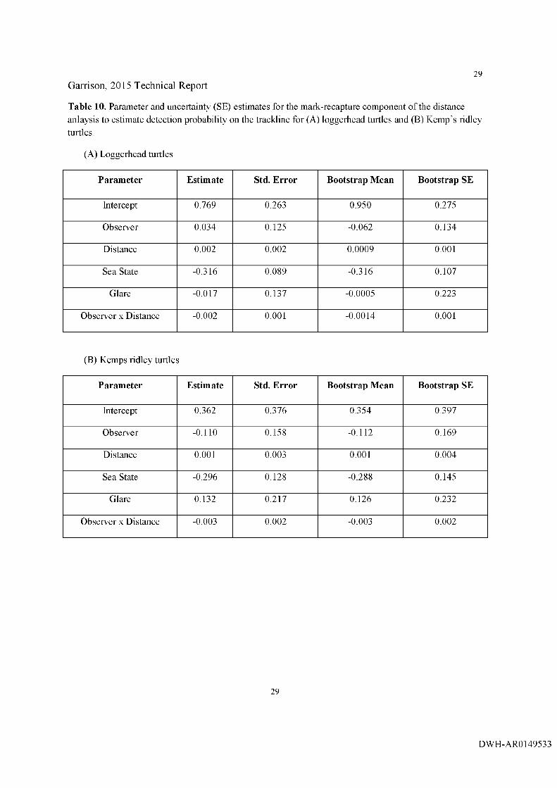
29Garrison, 2015 Technical Report
Table 10. Parameter and uncertainty (SE) estimates for the mark-recapture component o f the distance anlaysis to estimate detection probability on the trackline for (A) loggerhead turtles and (B) Kemp’s ridley turtles.
(A) Loggerhead turtles
Parameter Estimate Std. Error Bootstrap Mean Bootstrap SE
Intercept 0.769 0.263 0.950 0.275
Observer 0.034 0.125 -0.062 0.134
Distance 0.002 0.002 0.0009 0.001
Sea State -0.316 0.089 -0.316 0.107
Glare -0.017 0.137 -0.0005 0.223
Observer x Distance -0.002 0.001 -0.0014 0.001
(B) Kemps ridley turtles
Parameter Estimate Std. Error Bootstrap Mean Bootstrap SE
Intercept 0.362 0.376 0.354 0.397
Observer -0.110 0.158 -0.112 0.169
Distance 0.001 0.003 0.001 0.004
Sea State -0.296 0.128 -0.288 0.145
Glare 0.132 0.217 0.126 0.232
Observer x Distance -0.003 0.002 -0.003 0.002
29
DWH-AR0149533

30Garrison, 2015 Technical Report
Table 11. Loggerhead turtle habitat model parameters and selction. Explanatory terms for the count and binomial components o f the zero-inflated negative binomial model were selected based upon the minimum Akaike’s Information Criterion (AlC) among competing models. Model terms indicated in bold were statistically significant (p < 0.05).
Model Count Model Terms Binomial Model Terms AIC AAIC
0z + z.2 -H X + x.2 + y + y.2 -1- dfs + sst -1- CHL + ju l -1-
JUL.2 + JU1.3
z + z.2 + X + x.2 -1- y -1- Y.2 -1- dfs -1- sst -1- CHL -1- JUL
-H JU L .2 -H jul.3
3104 10
1z + z.2 + X + x.2 + Y + y.2
C H L j u l JUL.2 +
ju l.3
z + z.2 + X + x.2 -1- y -1- Y.2 + CHL + JUL + JUL.2 +
ju l.3
3101 7
2X -1 x.2 Y -r y.2 CHL
-i-jul + JUL.2 + jul.3X + X.2 + Y + Y.2 + CHL
-H JU L -H JU L .2 -Hjul.33124 30
3X x.2 Y y.2 CHL
-I- jul -1- JUL.2 -1-jul.3
z -1- z.2 -1- X -1- x.2 -1- y -1- Y.2 + CHL + JUL + JUL.2 +
jul.33097 3
4X -H x.2 -H Y -H y.2 -H CHL
-I-jul -1- JUL.2 -1-jul.3z-HZ.2-Hy-hY.2-HCHL-H
JUL-h JUL.2-h jul.33094 0
Model term defintions:z, Z.2 - depth and depth squared; x, x.2 - east-west coordinate and squared term; y, y.2 - north-south coordinate and squared term; dfs - distance from shore; sst - sea surface temperature; chi - surface chlorophyll; ju l,ju l.2, jul3 -Ju lian day and second and third order terms.
30
DWH-AR0149534

31Garrison, 2015 Technical Report
Table 12. Kemp’s ridley turtle habitat model parameters and selction. Explanatory terms for the count and binomial components o f the zero-inflated negative binomial model were selected based upon the minimum Akaike’s Information Criterion (AIC) among competing models. Model terms indicated in bold were statistically significant (p < 0.05).
Model Count Model Terms Binomial Model Terms AIC AAIC
0 z + Z.1 + x+ x.2 -H y -1- y.2 + dfs + sst -H CHL -H JUL -H jul.2 + jul.3
z + Z.2 + X + X.2 + y + Y.2 + DFS+ sst + CHL + jul -H JUL.2 -H jul.3
2264 9
I z + Z.2 + x+ X.2 + y + y.2 + dfs + c h i+ JUL-Hjul.2+jul.3
Z + Z.2 + X -H X.2 -H y -H y.2 -H DFS CHL jul JUL.2 + jul.3
2263 8
2 z + z.2 + x+ X.2 + y + y.2 + CHL + jul -H JUL.2 + jul.3
z + Z.2 + X X.2 y -h y.2 DFS-H CHL -H jul -H JUL.2 + jul.3
2261 6
3 X -H X.2 -H CHL -H jul + JUL.2 -H jul.3
Z -H Z.2 + X + X.2 -H y + y.2 + CHL DFS-Hjul-H J UL . 2 j u l . 3
2260 5
4chi -t JUL + jul.2 + jul.3
Z+ Z.2 + X + X.2 y + y.2 + CHL-I-jul -I- JUL.2 + jul.3
2263 8
5 X -H X.2 -H CHL -H jul + JUL.2 -Hjul.3
Z -H Z.2 -H X -H X.2 -H CHL -H dfs -H jul-H JUL.2-H jul.3
2255 0
Model term defintions:z, z.2 - depth and depth squared; x, x.2 - east-west coordinate and squared term; y, y.2 - north-south coordinate and squared term; dfs - distance from shore; sst - sea surface temperature; chi - surface chlorophyll; jul, jul.2, jul3 - julian day and second and third order terms.
31
DWH-AR0I49535

32Garrison, 2015 Technical Report
Table 13. Estimates o f injured and exposed turtles in the neritic habtiat for (A) loggerhead turtles, (B)
Kemp’s ridley turtles, and (C) unidentified hardshell turtles.
(A) Loggerhead turtles
Weeks Survey High Exposed 95% Cl Less Exposed 95% Cl28Apr-13May 28Apr-10May 0 - 12552 8610- 1769514May-28May 20May-24May 249 129-375 3913 1932 - 762929May-l lJun 07Jun-13Jun 412 143 - 725 3742 1255 - 899112Jun-26Jun 07Jun-13Jun 412 143 - 725 3742 1255 -899127Jun-10Jul 08Jul-21Jul 484 193 - 827 1089 698 - 15701 lJul-24Jul 08Jul-21Jul 484 193 - 827 1089 698 - 157025Jul-7Aug 22 Jul-31 Jul 174 0 -4 1 0 1498 945 - 2098
Total 2215 7 9 9 -3 8 8 7 27624 15391 -48453
(B) Kemp’s ridley turtles
Weeks Survey High Exposed 95% Cl Less Exposed 95% Cl28Apr-13May 28Apr-10May 0 - 6319 3315 - 1084414May-28May 20May-24May 148 0 -4 0 3 1692 9 1 4 -2 6 1 029May-l lJun 07Jun-13Jun 592 174 - 1499 2732 1482 - 454412Jun-26Jun 07Jun-13Jun 592 174 - 1499 2732 1482 - 454427Jun-10Jul 08Jul-21Jul 149 0 -4 4 0 651 171 - 12301 lJul-24Jul 08Jul-21Jul 149 0 -4 4 0 651 171 - 123025Jul-7Aug 22 Jul-31 Jul 59 0 -2 1 5 4169 2533 - 6439
Total 1689 349 - 4496 18945 10068 -31441
(C) Hardshell turtles
Weeks Survey High Exposed 95% Cl Less Exposed 95% Cl28Apr-13May 28Apr-10May 0 - 1940 9 1 7 -3 2 5 214May-28May 20May-24May 0 - 809 341 - 150329May-l 1 Jun 07Jun-13Jun 71 0 -1 6 8 393 177-69112Jun-26Jun 07Jun-13Jun 71 0 -1 6 8 393 177-69127Jun-10Jul 08Jul-21Jul 244 34 - 607 595 164-11811 lJul-24Jul 08Jul-21Jul 244 33 - 607 595 164-118125Jul-7Aug 22 Jul-31 Jul 0 - 510 148 - 975
Total 631 67 - 1550 5235 2088 - 9473
32
DWH-AR0149536

33Garrison, 2015 Technical Report
T able 14. Estimates o f injured and exposed turtles in the neritic habtiat for ages 1 -3 Kemp’s ridley turtles.
Age EstimatedAbundance
TotalArea(km^)
Density(N/km^)
Avg Oil Area (km2)
NumberExposed
Probability of being heavily
oiled
Numberheavily
oiled
1 77122 38900 1.98 4430 8783 0.044 3393
2 25836 38900 0.66 4430 2942 0.044 1137
3 8655 38900 0.22 4430 986 0.044 381
33
DWH-AR0149537

34Garrison, 2015 Technical Report
Figure 1. Spatial extent of synoptic aerial surveys conducted during April - September 2010. All “on
effort” trackline segments are shown. Portions of tracklines in waters > 200m depth were excluded from
this analysis.
91’30'W 91’0'W 90’30'W 90°0WJ _____________ I_____________ 1_____________ t_
l"30W 89°0W 88°30W 88’0'W 87'30'W 87’OWJ _____________ I_____________ I_____________ I_____________ I_____________ 1_
Synoptic Aerial Survey Extent
^ DWH Rig Location
[ J Survey Area
■ Trackiines
200 meter isobath
90"30W 90"0W 89"30'W 89’0'W
34
DWH-AR0149538

Garrison, 2015 Technical Report
Figure 2. Spatial extent of seasonal broadscale aerial surveys flown during 2011-2012.
35
98^0'W J__ 96^0'WI 94^0'WI
92"0WI
90'0WI
86^0'W 1
drowI 82°0'W
200 m eter isobath
96°0'W 9ro'w 92°0'W 90°0'W
Broadscale Aerial Survey Extent
Survey Effort
"i Broadscale S trata
86°0'W srow 82^0'W
35
DWH-AR0149539

36Garrison, 2015 Technical Report
Figure 3. Initial tagging locations o f loggerhead and Kemp’s ridley turtles included in the analysis of dive-surface behaviors.
82^0'W96“0W 1
9 2 V W 1
9 0 V W 1
86°0W I
8ro'w
Initial Turtle Tagging Locations200 meter isobath
Initial Location S p ec ie s
A Kemp's Ridley
© Loggerhead
94°0W 92°0W 90°0W 86°0'W srow 82°0'W
36
DWH-ARO149540

Garrison, 2015 Technical Report
Figure 4. Grid area (10 x 10 km cells) used for habitat models of animal density.
37
9 r3 0 'W 9 r o 'w 90°30W 90VW 89'^30'W f'30W row 87'^30W 87^0W
Spatial Prediction Grid
200 m eter isobath
I I Prediction Grid
-P
>30W >0'W
37
DWH-ARO 149541

38Garrison, 2015 Technical Report
Figure 5. Survey effort and turtle sightings for sj^noptic surveys. (A) Survey 1
n 'M y v 91'v w 9 tr» y v 9 0 v w M 'so w t f o w w j o w c r tr w $r3oyv t r o w
S ynoptic Survey Effort and S igh tin gs
SpeciesKemp's Ridley
Logpeftieed
Treckknes
200 m e ten so M h
T s
t f» w wow 9ffow e r» w wow i r» w wow »r3ow trow
(B) Survey 29f*30W trovf W30W 90*0W t9'J01V «7‘30W 87'OW
S y n o p tic S urvey Effort and S ig h tin g s
SpeciesKemp s Ridley
A Loggerhead
i|
tf30w »row 66'0'w 67'x w erew
(C) Survey 39f’J0W »f*OW K ’XW WOW M'30W WOW W30W «'0W arjow t r w
S y n o p tic S u r v ey Effort an d S ig h tin g s
SpeciesKemp'S RKiiey
U>ggert>esd
Tracklines
200 m eter isobath
87-X-W 87‘Oyf
38
DWH-ARO 149542

Garrison, 2015 Technical Report
Figure 5 cont. Survey effort and turtle sightings for synoptic surveys.(D) Survey 4
39
vrjow titrw tcrxw ktow m x n r m trw aram r arm v e rx y v
S y n o p tic S urvey Effort and S ig h tin g s
Species _ Kemp’s RKNey
▲ LoQoeftteed Trackhne*
200 nteterisobsth
)
x 'x w »rov¥ M 'xvf ao’ow 8e*»w arcw $ r x w tro w
(E) Survey 59fOW X'XW K'OW 99’30’W tfOW tt'X W tfOW 87'XW 87'OW
S y n o p tic S urvey Effort and Sightings
S p e c ie s
a . Kemp's Ridley
Loggerhead
Tracklines
200 m eter isobath
to'ow aa'so’vv t fo w t7 'x w
(F) Survey 6o r x w orow oo-30iv flo-o’W' w x w tfo w X'ow t r x w bt'ow
S y n o p tic S urvey Effort and S ig h tin g s
SpeciesKemp's Ridley
A Loggerhead
Tracklines
200 m eter isobatti
91'XW 01‘OW x - x w X'OW W'XW M'OW Bt'XW t r x w t7-ow
39
DWH-ARO 149543

40Garrison, 2015 Technical Report
Figure 5 cont. Survey effort and turtle sightings for synoptic surveys.
(G) Survey 796'30'W 96 'o w « r » w $ r v w
S y n o p tic S urvey Effort and S ig h tin g s
SpeciesKemp's Ridley
Loggertieed
T iacklnes
r i J T t i f f n
40
DWH-AROl 49544

Garrison, 2015 Technical Report
Figure 6. Survey effort and turtle sightings for seasonal broadscale surveys.
(A) Spring 2011
41
8 2 V W9 8 V W 96’OW I 9 4 V W I
92‘OW I
9 0 V W 1
86VW 1
B ro a d sc a le A erial S u rv ey S ig h tin g s
Sightings: Spring 2011 Species
A Kem p's Ridley
C Loggerhead
Effort: Spring 2011
86'OW9 8 V W 9 6 V W 94VW 92 V W 9 0 V W 82 OW
(B) Summer 2011
98 0W 96 0'W I 9ro'wI 92^0'W 1
90^0'W I
Bro'wI 82“0W
B ro a d sc a le A erial S u rv e y S ig h tin g s
Sightings: Summer 2011 Species
A Kemp's Ridley C Loggerhead
Effort: Sum m er 2011
41
DWH-ARO 149545

Garrison, 2015 Technical Report
Figure 6 cont. Survey effort and turtle sightings for seasonal broadscale surveys.
(C) Fall 2011
42
98’OW J- 96°0W 9 r o w _i_ 92'OW _l_ 90°0W _ L
88^0'W i_
94 OW
B ro a d sc a le Aerial S u rv ey S ig h tin g s
Sightings: Fall 2011S p e c i e s
A K em p 's Ridley
O L ogg erh ead
Effort: Fall 2011
98^0'W 96°0W 9rO'W 92°0W 90°0W drow 82'^0'W
(D) Winter 2012
82^0'W98'^0'W 96'^0'W I 9ro'wI 92'^O'W I
90'^0'W 1
86 "OW 1
94 “OW
B ro a d sc a le A erial S u rv ey S ig h tin g s
Sightings: Winter 2012Species A K em p 's R idley
C L o g g erh ead
Effort: W inter 2011
88°0'W98“6W 96^0'W 92“0W QOO'W 86°0'W drew 82^0'W
42
DWH-AR0149546

Garrison, 2015 Technical Report
Figure 7. Daily best tag locations and tracks for loggerhead (A) and Kemp’s ridley (B) turtles.
(A) Loggerhead
43
980'Wr l -
96^0'W oro'wJ -
92^0'W 90^0'W _L
86 “OW 1
drowI 82^0W
Daily Turtle Tag Locations• Daily Locations; Loggerhead
Tag Tracks: Loggerhead
200 meter isobath
98°0W 96 0W 9rO'W 92°0’W 90VW 88VW 86VW srow arow
(B) Kemp’s ridley
98°0W J__ 96°0W■ 94°0WI 92°Q’WI 90°0WI 88°0W 82°0W86°0W srow
Daily Turtle Tag Locations▲ Dally Locations: Kemp's
Tag Tracks: Kemp's
200 meter Isobath
-1----rowrow 96^0W grow 92^0W 90^0W 86^0W srow 82*0W
43
DWH-ARO 149547

44Garrison, 2015 Technical Report
Figure 8. Fitted and observed detection probabilities for duplicate sightings o f (A) loggerhead and (B) Kemp’s ridly turtles during broadscale aerial sun^eys. The line indicates the population mean detection probability while points indicate predicted detection probahility for covariate combinations (i.e., sea state, glare).
(A) Loggerhead turtles
CDJUO
05
Q
o
COo
OOO 0 0 0 0 o 0 o
o
CMo
oo
0 50 100 150 200 2 50 300
(B) Kemp’s ridley turtles
Distance
05Q
o
oqd
cix> °
oo'Jd i
r\io
od i
0 50 100 150 200 250 300
D is tan ce
44
DWH-ARO 149548

45Garrison, 2015 Technical Report
Figure 9. Detection functions for (A) loggerhead turtles and (B) Kemp’s ridley turtles during synoptic surveys.
(A) Loggerhead turtles
ii
o
ci Ip
50 100 150 200 250 300
D istance
(B) Kemp’s ridley turtles
COo
o
50 100 150 200 250 300
D istance
(C) Unidentified hardshell turtles
0 50 1 00 1 50 2 00 2 50 300
D istance
45
DWH-AROl 49549

46Garrison, 2015 Technical Report
Figure 10. Box-whisker plots of (A) loggerhead turtle, (B) Kemp’s ridley turtle, and (C) unidentfieid hardshell turtle abundance during the 2010 sjmoptic surveys from the bootstrap distribution o f estimates. The upper and lower borders o f the boxes reflect the 75* and 25* percentiles, and the dark line is the median. The “notch” in each box reflects the range o f the 95% confidence interval while the “whiskers” reflect the range o f the data exlcuding outliers (points).
(A) Loggerhead turtles
oOOOUP
ooooo
ooooU9
2BApr-1 OMay 20May-24May 07Jun-13Jun 25Aug-02Sep
+= o
EDz
Survey Dates
(B) Kemp’s ridley turtles
28Apr-10May 20May-24May 0TJun-13Jun 08JuH2Jul
Sur\'ey Datss
22Juh31Jul 25Aug-02Sep
46
DWH-AR0149550

47Garrison, 2015 Technical Report
(C) Unidentified hardshell turtles
OOlOro
oooif)OJ
oooLO
O
28Apr-10May 20May-24May 07Jun-13Jun 08Jul-12Jul 22Jul-31Jul 25Aug-02Sep
Survey Dates
47
DWH-AR0149551

Garrison, 2015 Technical Report
Figure 11. Predicted loggerhead turtle abundance in 10 x 10 km grid cells during synoptic sui^^eys.
(A) Survey 1 (B) Survey 2
48
Loggerhead Turde Abundance
(C) Survey 3 (D) Survey 4
Loggerhead lurae Abundance
Survey 3 nrOeuCell
(E) Survey 5 (F) Survey 7
Loggerhead mrfle Abundance
Survey e TMOtWCell
Loggerhead Turtle Abundance
48
DWH-AR0149552
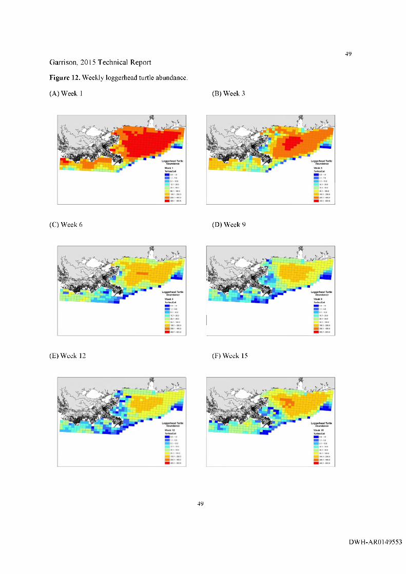
Garrison, 2015 Technical Report
Figure 12. Weekly loggerhead turtle abundance.
(A) Week 1 (B) Week 3
49
Loggerhesd Tunl« Abundance
Loggerhead Turtle Abundance
(C) Week 6 (D) Week 9
Loggerhead lUrOe Abundance
Loggerhead TUrde Abundance
(E) Week 12 (F) Week 15
'•.sV
Loggerhead Turbe Abundartce
49
DWH-AR0149553

50Garrison, 2015 Technical Report
Figure 13. Predicted Kemp’s ridley turtle abundance in 10 x 10km grid cells during synoptic surveys.
(A) Survey 1 (B) Survey 2
Surve/ 1 Survey 2 TunietA tri
(C) Survey 3 (D) Survey 4
s rlrtley
(E) Survey 5 (E) Survey 7
t rlrtley TUrQe AburxlarKe
Survey 5 Turtie«<CeH
• rklley TUrOe Abundance
Survey 7 Tuniee/C
50
DWH-AR0149554

Garrison, 2015 Technical Report
Figure 14. Weekly Kemp’s ridley turtle abundance.
(A) Week 1 (B) Week 3
51
K em pt rMiey Turtle AJwndance
Hemp's ndley Turtle AtMrtdance
(C) Week 6 (D) Week 9
Kemp s ndtey Turtle Abundance
(E) Week 12 (F) Week 15
Kemp s ndtey Turtle Abundance
Kemp s ndtey TurPe Abundance
51
DWH-AR0149555

52Garrison, 2015 Technical Report
Figure 15. Weekly abundance o f (A) loggerhead and (B) Kemp’s ridley turtles predicted from spatial habitat models.
(A) Loggerhead
U, 180000 H ■O (O 0) 160000 -.c(UboboO
kl—o
140000 -
120000 -
^ 100000 - OJE 80000 -
2 60000 -■a0)4->„ 40000 -
^ 20000 -(/)LU
0 2 6 8 10 12 14 16 184
(B) Kemp’s ridley
Week
^ 180000 I 160000-a 140000
12000010000080000600004000020000V)
0 8 10 Week
12 14 16 18
52
DWH-AR0149556