Garfield, a drift-chamber simulation program User's …lambda.phys.tohoku.ac.jp/~kobayash/seminar/files/cern/...Garfield, a drift-chamber simulation program User's guide Version 4.29

Garfield, a drift-chamber simulation programUser's guideVersion 4.29

30 November 1993

Rob Veenhof

Garfield is a computer program for the detailed simulation of two-dimensional drift chambers. The program can forinstance calculate field maps, x(t) relations, arrival time distributions, induced signals and the drift velocity anddiffusion in gas mixtures. Garfield can also assist in optimising the potential settings.

Garfield, a drift-chamber simulation program

User's guide

Version 4.29

Garfield, a drift-chamber simulation program

User's guide

Version 4.29

Copyright notice

© Rob Veenhof, 1993, all rights reserved.

Garfield, a drift-chamber simulation program, CERN Program Library entry W5050

Copyright and any other appropriate legal protection of this computer program and associated documentationreserved in all countries of the world.

This program or documentation may not be reproduced and/or redistributed by any method without prior writtenconsent of the author.

Permission for the scientific usage of any programs described herein is granted apriori to those scientific insti-tutes associated with the CERN experimental program or with whom CERN has concluded a scientific collab-oration agreement.

Commercial utilisation requires explicit a priori permission from the author and will be subjected to payment ofa license fee.

Submitter: M.MarquinaLanguage: FORTRANLibrary: POOL-W5050

ii Garfield, a drift-chamber simulation program

What is Garfield ?

Garfield tries to simulate the behaviour of drift-chambers: it calculates and plots the electrostatic field, the drift-lines of electrons and ions and the currents on the sense wires resulting from the passage of a charged particlethrough the chamber. The program can also assist you in finding optimal potential settings under certain con-straints. For calibration purposes, Garfield can compute x(t)-relations and arrival time distributions.

The program is primarily meant for use with chambers that consist only of thin wires and infinite equipotentialplanes. Periodicity, magnetic fields and cylindrical geometry are allowed. Fancy electrodes can only be handled byapproximation. Garfield can not deal with three-dimensional structures.

Garfield can be run interactively and in batch on most of the CERN central computers. One of the main features ofthe program is probably its friendliness; little knowledge about the computer system and no knowledge at all aboutprogramming languages is required to be able to run it.

What is Garfield ? iii

iv Garfield, a drift-chamber simulation program

Contents

1.0 Introduction . . . . . . . . . . . . . . . . . . . . . . . . . . . . . . . . . . . . . . . . . . . . . . . . . . . . 11.1 What the program can do . . . . . . . . . . . . . . . . . . . . . . . . . . . . . . . . . . . . . . . . . . . . . 11.2 What the program cannot do . . . . . . . . . . . . . . . . . . . . . . . . . . . . . . . . . . . . . . . . . . . 11.3 In case of problems ... . . . . . . . . . . . . . . . . . . . . . . . . . . . . . . . . . . . . . . . . . . . . . . . 2

2.0 Running the program . . . . . . . . . . . . . . . . . . . . . . . . . . . . . . . . . . . . . . . . . . . . . . . 32.1 How to start the program on each of the systems . . . . . . . . . . . . . . . . . . . . . . . . . . . . . . . . 3

2.1.1 Running on Apollo and Unix systems . . . . . . . . . . . . . . . . . . . . . . . . . . . . . . . . . . . . 32.1.2 Running on the Cray . . . . . . . . . . . . . . . . . . . . . . . . . . . . . . . . . . . . . . . . . . . . . 42.1.3 Running under VM/CMS and Cray job submission . . . . . . . . . . . . . . . . . . . . . . . . . . . . 42.1.4 Running on Vax/VMS . . . . . . . . . . . . . . . . . . . . . . . . . . . . . . . . . . . . . . . . . . . . 8

2.2 Terminal types . . . . . . . . . . . . . . . . . . . . . . . . . . . . . . . . . . . . . . . . . . . . . . . . . . . 92.3 Datasets . . . . . . . . . . . . . . . . . . . . . . . . . . . . . . . . . . . . . . . . . . . . . . . . . . . . . . . 9

2.3.1 Garfield output datasets . . . . . . . . . . . . . . . . . . . . . . . . . . . . . . . . . . . . . . . . . . . . 102.3.2 File naming conventions and input file format . . . . . . . . . . . . . . . . . . . . . . . . . . . . . . . 10

2.4 Error messages . . . . . . . . . . . . . . . . . . . . . . . . . . . . . . . . . . . . . . . . . . . . . . . . . . . 122.4.1 Garfield messages . . . . . . . . . . . . . . . . . . . . . . . . . . . . . . . . . . . . . . . . . . . . . . . 122.4.2 GKS error messages . . . . . . . . . . . . . . . . . . . . . . . . . . . . . . . . . . . . . . . . . . . . . 132.4.3 Fortran run-time error messages . . . . . . . . . . . . . . . . . . . . . . . . . . . . . . . . . . . . . . . 13

3.0 Program input . . . . . . . . . . . . . . . . . . . . . . . . . . . . . . . . . . . . . . . . . . . . . . . . . . . 153.1 Input format . . . . . . . . . . . . . . . . . . . . . . . . . . . . . . . . . . . . . . . . . . . . . . . . . . . . 153.2 Control structures . . . . . . . . . . . . . . . . . . . . . . . . . . . . . . . . . . . . . . . . . . . . . . . . . . 16

3.2.1 Global variables . . . . . . . . . . . . . . . . . . . . . . . . . . . . . . . . . . . . . . . . . . . . . . . . 173.2.2 IF-blocks and IF-lines . . . . . . . . . . . . . . . . . . . . . . . . . . . . . . . . . . . . . . . . . . . . 173.2.3 DO-loops . . . . . . . . . . . . . . . . . . . . . . . . . . . . . . . . . . . . . . . . . . . . . . . . . . . 183.2.4 Procedure calls . . . . . . . . . . . . . . . . . . . . . . . . . . . . . . . . . . . . . . . . . . . . . . . . 18

3.3 Physical units . . . . . . . . . . . . . . . . . . . . . . . . . . . . . . . . . . . . . . . . . . . . . . . . . . . . 193.4 The cell section . . . . . . . . . . . . . . . . . . . . . . . . . . . . . . . . . . . . . . . . . . . . . . . . . . . 213.5 The magnetic field section . . . . . . . . . . . . . . . . . . . . . . . . . . . . . . . . . . . . . . . . . . . . . 273.6 The gas section . . . . . . . . . . . . . . . . . . . . . . . . . . . . . . . . . . . . . . . . . . . . . . . . . . . 28

3.6.1 Built-in gasses . . . . . . . . . . . . . . . . . . . . . . . . . . . . . . . . . . . . . . . . . . . . . . . . . 283.6.2 Entering a description of the gas . . . . . . . . . . . . . . . . . . . . . . . . . . . . . . . . . . . . . . . 30

3.7 The optimisation section . . . . . . . . . . . . . . . . . . . . . . . . . . . . . . . . . . . . . . . . . . . . . . 393.8 The field section . . . . . . . . . . . . . . . . . . . . . . . . . . . . . . . . . . . . . . . . . . . . . . . . . . 433.9 The drift section . . . . . . . . . . . . . . . . . . . . . . . . . . . . . . . . . . . . . . . . . . . . . . . . . . 493.10 The signal section . . . . . . . . . . . . . . . . . . . . . . . . . . . . . . . . . . . . . . . . . . . . . . . . . 663.11 The stop command . . . . . . . . . . . . . . . . . . . . . . . . . . . . . . . . . . . . . . . . . . . . . . . . 733.12 Instructions valid in all sections . . . . . . . . . . . . . . . . . . . . . . . . . . . . . . . . . . . . . . . . . 74

3.12.1 Global options . . . . . . . . . . . . . . . . . . . . . . . . . . . . . . . . . . . . . . . . . . . . . . . . 743.12.2 Kernlib error messages . . . . . . . . . . . . . . . . . . . . . . . . . . . . . . . . . . . . . . . . . . . 743.12.3 Printing a comment . . . . . . . . . . . . . . . . . . . . . . . . . . . . . . . . . . . . . . . . . . . . . 743.12.4 Comment lines . . . . . . . . . . . . . . . . . . . . . . . . . . . . . . . . . . . . . . . . . . . . . . . . 753.12.5 Input translation tables . . . . . . . . . . . . . . . . . . . . . . . . . . . . . . . . . . . . . . . . . . . 753.12.6 Obtaining help . . . . . . . . . . . . . . . . . . . . . . . . . . . . . . . . . . . . . . . . . . . . . . . . 763.12.7 Input from and output to datasets . . . . . . . . . . . . . . . . . . . . . . . . . . . . . . . . . . . . . 763.12.8 Shell commands . . . . . . . . . . . . . . . . . . . . . . . . . . . . . . . . . . . . . . . . . . . . . . . 763.12.9 Garfield library manipulation commands . . . . . . . . . . . . . . . . . . . . . . . . . . . . . . . . . 773.12.10 Graphics instructions . . . . . . . . . . . . . . . . . . . . . . . . . . . . . . . . . . . . . . . . . . . . 793.12.11 The algebra instruction list editor . . . . . . . . . . . . . . . . . . . . . . . . . . . . . . . . . . . . . 87

4.0 Description of the physical model . . . . . . . . . . . . . . . . . . . . . . . . . . . . . . . . . . . . . . . . 914.1 Electrostatics, magnetostatics . . . . . . . . . . . . . . . . . . . . . . . . . . . . . . . . . . . . . . . . . . . 91

4.1.1 Notation . . . . . . . . . . . . . . . . . . . . . . . . . . . . . . . . . . . . . . . . . . . . . . . . . . . . 91

Contents v

4.1.2 Cell types . . . . . . . . . . . . . . . . . . . . . . . . . . . . . . . . . . . . . . . . . . . . . . . . . . . 924.1.3 Isolated charges (type A) . . . . . . . . . . . . . . . . . . . . . . . . . . . . . . . . . . . . . . . . . . . 934.1.4 Rows of charges (types B1x, B1y, B2x and B2y) . . . . . . . . . . . . . . . . . . . . . . . . . . . . . 934.1.5 Electrostatic field of a doubly periodic wire array . . . . . . . . . . . . . . . . . . . . . . . . . . . . . 954.1.6 Isolated charges in a tube (type D1) . . . . . . . . . . . . . . . . . . . . . . . . . . . . . . . . . . . . 1024.1.7 Ring of charges in a tube (type D2) . . . . . . . . . . . . . . . . . . . . . . . . . . . . . . . . . . . . 1024.1.8 The capacitance equations, boundary conditions . . . . . . . . . . . . . . . . . . . . . . . . . . . . . 1024.1.9 Cylindrical geometry, internal coordinates . . . . . . . . . . . . . . . . . . . . . . . . . . . . . . . . 1034.1.10 Zeros of the electric field . . . . . . . . . . . . . . . . . . . . . . . . . . . . . . . . . . . . . . . . . 1044.1.11 Magnetic field calculation . . . . . . . . . . . . . . . . . . . . . . . . . . . . . . . . . . . . . . . . . 105

4.2 Mixing gasses . . . . . . . . . . . . . . . . . . . . . . . . . . . . . . . . . . . . . . . . . . . . . . . . . . 1054.3 Motion of electrons and ions . . . . . . . . . . . . . . . . . . . . . . . . . . . . . . . . . . . . . . . . . . 110

4.3.1 The equation of motion . . . . . . . . . . . . . . . . . . . . . . . . . . . . . . . . . . . . . . . . . . . 1104.3.2 Numerical solution of the equation of motion . . . . . . . . . . . . . . . . . . . . . . . . . . . . . . 1114.3.3 Calculation of x(t)-relations . . . . . . . . . . . . . . . . . . . . . . . . . . . . . . . . . . . . . . . . 112

4.4 Signal simulation . . . . . . . . . . . . . . . . . . . . . . . . . . . . . . . . . . . . . . . . . . . . . . . . . 1124.4.1 Track generation . . . . . . . . . . . . . . . . . . . . . . . . . . . . . . . . . . . . . . . . . . . . . . 1124.4.2 Drift of the clusters towards the anode . . . . . . . . . . . . . . . . . . . . . . . . . . . . . . . . . . 1144.4.3 Calculation of the ion-tail . . . . . . . . . . . . . . . . . . . . . . . . . . . . . . . . . . . . . . . . . 115

4.5 Evaluation of symbolic formulae . . . . . . . . . . . . . . . . . . . . . . . . . . . . . . . . . . . . . . . . 1164.5.1 Guidelines . . . . . . . . . . . . . . . . . . . . . . . . . . . . . . . . . . . . . . . . . . . . . . . . . . 1174.5.2 Details about the translation process . . . . . . . . . . . . . . . . . . . . . . . . . . . . . . . . . . . . 117

5.0 Compiling the program . . . . . . . . . . . . . . . . . . . . . . . . . . . . . . . . . . . . . . . . . . . . . 1235.1 Obtaining the source file . . . . . . . . . . . . . . . . . . . . . . . . . . . . . . . . . . . . . . . . . . . . . 123

5.1.1 Distribution conditions . . . . . . . . . . . . . . . . . . . . . . . . . . . . . . . . . . . . . . . . . . . 1235.1.2 File location . . . . . . . . . . . . . . . . . . . . . . . . . . . . . . . . . . . . . . . . . . . . . . . . . 1235.1.3 Source file contents . . . . . . . . . . . . . . . . . . . . . . . . . . . . . . . . . . . . . . . . . . . . . 123

5.2 The YPATCHY step . . . . . . . . . . . . . . . . . . . . . . . . . . . . . . . . . . . . . . . . . . . . . . . 1245.3 Making the executable and related files . . . . . . . . . . . . . . . . . . . . . . . . . . . . . . . . . . . . 126

5.3.1 UNIX . . . . . . . . . . . . . . . . . . . . . . . . . . . . . . . . . . . . . . . . . . . . . . . . . . . . 1265.3.2 VM / CMS . . . . . . . . . . . . . . . . . . . . . . . . . . . . . . . . . . . . . . . . . . . . . . . . . 1275.3.3 Vax/VMS . . . . . . . . . . . . . . . . . . . . . . . . . . . . . . . . . . . . . . . . . . . . . . . . . . 127

6.0 Details about the program . . . . . . . . . . . . . . . . . . . . . . . . . . . . . . . . . . . . . . . . . . . 1296.1 I/O units . . . . . . . . . . . . . . . . . . . . . . . . . . . . . . . . . . . . . . . . . . . . . . . . . . . . . . 1296.2 Debugging . . . . . . . . . . . . . . . . . . . . . . . . . . . . . . . . . . . . . . . . . . . . . . . . . . . . 1296.3 Brief description of all routines . . . . . . . . . . . . . . . . . . . . . . . . . . . . . . . . . . . . . . . . . 1296.4 Program history . . . . . . . . . . . . . . . . . . . . . . . . . . . . . . . . . . . . . . . . . . . . . . . . . 141

7.0 Acknowledgments . . . . . . . . . . . . . . . . . . . . . . . . . . . . . . . . . . . . . . . . . . . . . . . . 143

Bibliography . . . . . . . . . . . . . . . . . . . . . . . . . . . . . . . . . . . . . . . . . . . . . . . . . . . . . 147

Index . . . . . . . . . . . . . . . . . . . . . . . . . . . . . . . . . . . . . . . . . . . . . . . . . . . . . . . . . . 149

vi Garfield, a drift-chamber simulation program

1.0 Introduction

1.1 What the program can doGarfield operates on drift-chambers made up of thin wires, up to two, not necessarily grounded, planes at constant xor r and up to two, not necessarily grounded, planes at constant y or φ. Infinite repetition of the cell in x and in y(or φ) can be taken into account. Radial repetition is not supported for technical reasons. The description of thechamber can either be in polar or in Cartesian coordinates and consists of a listing of the wire positions, potentialsand diameters, of the plane positions and potentials, of the periodicities and of the dielectrica.

When doing drift line calculations, the program further needs a detailed description of the gas. This description canbe provided by the user, but some frequently used gasses are built in the program (CO2, methane, ethane, isobutane,argon-ethane, CO2-ethane etc.). Garfield can also calculate the drift velocity and the diffusion in gas mixtures.

The tasks Garfield can perform, include the following:

• Plotting of (almost) any function of the field as a histogram, a vector plot, a set of contour lines, a 3 dimen-sional surface or a graph. The field in a given part of the chamber and on the surface of a group of wires canbe tabulated. A command is provided that checks that the potential and the field are consistent, satisfyMaxwell's equations and satisfy the boundary conditions.

• Assisting you in finding optimum potential settings under a variety of constraints. The dependency of the fieldon the wire potentials can be printed.

• Calculation and plotting of electron and ion drift-lines and equal arrival time contours. The drift-lines may startat the wire-surface, at the edge of a user-defined drift-area or from a user-defined track. In the latter case,graphs of the drift-time, the mean drift-speed, the integrated diffusion and of the multiplication factor are madeon request.

• Calculation of x(t)-relations, if required for inclined tracks, optionally estimating the longitudinal diffusion.The case your equipment counts electrons before it triggers is also handled by the program. Garfield canproduce drift-time tables.

• Simulation of the signal induced on the sense wires when a charged particle traverses the cell. The effectswhich can be taken into account are: cluster-formation, longitudinal diffusion, avalanche near the wire-surface,electron-pulse and the ion-induced current. The simulated signal can be used as an input to the electronicscircuitry simulation programs Spice or Sceptre.

A variety of routines to obtain data derived from field and drift-line calculations is available and it should thereforenot be difficult for a user to write his/her own extensions.

1.2 What the program cannot doThe major limitations of the program are:

• All calculations are carried out in the thin-wire approximation, hence the wire-spacing should be at least 5-10times the wire radius. Corrections such as dipole and quadrupole terms might be included in some futureversion.

• Strips or line-electrodes of finite length have to be replaced by rows of wires of appropriate diameter. You'llhave to use another program if such an approximation is not adequate.

• Only infinite slabs of dielectric material will be handled by Garfield in a future release. Programs using finiteelement methods like Poisson will probably suit you better if dielectrica are an important component of yourchamber.

• The program input allows only for simple, uniform magnetic fields but the distortion of the magnetic field dueto the difference in susceptibility between the gas and the wire-material can be taken into account. This is nota true limitation since the user may provide her/his own routine returning the magnetic field if he/she wishes todo so.

Introduction 1

• The program neglects lateral diffusion in its present version. This is not a fundamental limitation and it isconceivable that future versions will know about lateral diffusion, should there be sufficient interest (pleasesend a message to the author).

• The field-calculation is 2-dimensional in an essential way. The main reason for this limitation is that analyticpotentials for such simple configurations as two crossing wires, are not known. One should therefore use afinite element method program, such as TOSCA, whenever the chamber is truely 3-dimensional. Extending thedrift-line routines to 3-dimensional situations is trivial and has been done to some extent in the current version.

• The program is not noted for its speed ! If the number of wires is large (over 1000) running Garfield may nolonger be practicable; again Poisson or similar programs might be more like what you need. Sometimes, theefficiency can greatly be increased by making the chamber periodic, at least part of it. The number of wireskept in mind while writing the program, is about 50. Tests have been done up to 1000 wires.

On some machines special compilations are available that make effective use of the vector facilities, makingcomputations on chambers with 1000 wires feasible again.

• The author can not warrant correct functioning of any part of the program, it is the duty of the user to checkthat the accuracy of the results is adequate for her/his purposes !

1.3 In case of problems ...A common source of problems is the use of an old manual with a new version of the program. While this maysometimes work, it should be kept in mind that Garfield changes continuously, trying to adapt to the needs of itsusers. No attempt is made to maintain backwards compatibility.

The best strategy is to contact me if you plan to make extensive use of the program. This allows me to keep trackof the kind of thing the program is used for and to make the program better suited for your applications. I can thenalso warn you in case a serious bug is found.

Please tell me if you have suggestions for improvement. Great efforts have been made to make the program itselfunderstandable because bugs are bound to be present. However, even if you manage to correct them, please send amessage. My electronic mail addresses are:

VM/CMS at CERN: RJD@CERNVMCERN central Vax: VXCERN::VEENHOF

Conventional mail can be sent to:

Rob Veenhof Rob VeenhofCERN /PPE-division 2, Rue du ReculetCH-1211 Genève 23 F-�163� St Genis-PouillySwitzerland / Suisse Francetel: + 41 22 7673897 tel: + 33 5�421784Fax: + 41 22 783�672

G.A. Erskine, who contributed essential routines and ideas, should not be called when problems occur. The personto contact in case of control-C problems on the Vax, is Carlo Mekenkamp.

I greatly appreciate receiving a copy of any note or publication for which this program has been used.

2 Garfield, a drift-chamber simulation program

2.0 Running the program

If you are not at CERN, you may have to compile and link Garfield yourself before you proceed. Instructions fordoing so can be found in Chapter 5.0 on page 123. This chaper assumes compilation has been done and describeshow you start the program. Other topics discussed are dataset usage and error messages.

2.1 How to start the program on each of the systemsAt CERN, and some other sites, you should not have any initialisation for Garfield in your profile, login commandprocedure etc. You may need some private initialisation for GKS.

The numerical parts of the program are identical on all machines; the plotting and I/O parts are definitely not. Theprogram behaviour and appearance of the output can therefore vary somewhat between the various systems.

Garfield can be run interactively and in batch on most computers. If you run the program interactively, theprogram will first do some initialisation and then wait for you to type a command, execute the command and waitfor the next. To stop the program, you have to enter the & STOP command. When Garfield is running in batch,the commands are taken from an input file and the program stops executing when the end of the input file isreached.

2.1.1 Running on Apollo and Unix systemsThe executable files for Garfield are stored in the usual CERN directories, nothing special has to be done thereforeto start the program. Garfield uses GKS and you may need to perform GKS initialisation as described in the CERNcomputer graphics guides. The format of the Garfield command is as follows:

$ garfield [-terminal {type T | GKS_id G connection_id C} ] [-noterminal]

[-metafile {type T | GKS_id G offset O name F} ] [-nometafile]

[-nodebug | -debug][-noidentification | noidentification][-RNDM_initialisation | -noRNDM_initialisation]

Note: all options and values have to be entered in the case shown. They may be abbreviated to some extent.

terminal Either specify the type, which can for instance be DN300_bw, DN3000_bw, DN3000_colour,DN550_colour, DN660_colour or X_windows_2 for GTS-GRAL compilations. Or the GKS_identifierand the connection_identifier both of which are numeric.

Use -noterminal if you wish to suppress all graphics output on the screen.

metafile The kind of metafile output can, like the terminal type, be specified either via type or via theGKS_identifier, the offset, which is the difference between the logical unit which the metafile is openedand the connection identifier, and the name, the name of the metafile. The metafile is by default inPostScript format, the alternatives are Encapsulated PostScript, a format suitable for inclusion in otherdocuments, and Appendix-E metafile, a format that is convenient for viewing the pictures on a terminallater on.

-debug Requests that debugging mode is initially on, that is, also during initialisation. This flag can beswitched off when the program is reading input by means of the OPTION command. Default is-nodebug.

-identification Requests that tracing is on from the start of program execution onwards, also during initialisation.Default is -noidentification.

-RNDM_initialisation When the program starts executing, it calls the RNDM random generator a number of timesthat depends on the time of the day. This ensures that results for which Monte-Carlo techniques areused, are produced with different random number sequences in each run. In case you wish to dodebugging, this may not be desirable; the -noRNDM_initialisation qualifier suppresses the initialisation.

Running the program 3

There are two ways on Unix to make Garfield read an input file: via the program's own < command and via theUnix < on the command line. There is an important difference between the two: when you type

$ garfieldMain: < input

all plots will be displayed on the screen and, unless the input file ends on a & STOP, further input can be enteredmanually. If on the other hand you type

$ garfield < input

Garfield behaves as if running in batch, and a metafile will be produced rather than pictures on the screen.

Surface plots and some contour plots can not be made on most Unix machines.

2.1.2 Running on the CrayEither log on to the Cray and start the program there:

/cern/pro/exe/garfield

and similarly for the OLD and NEW versions, or submit an input file from VM/CMS to the Cray. The latter is themore convenient method, see Section 2.1.3 for details.

Keep in mind that the NAG graphics library has not been compiled on this machine and that surface plots cantherefore not be made.

2.1.3 Running under VM/CMS and Cray job submissionType the following to start Garfield interactively:

(login sequence)GARFIELD

The news will appear after a few seconds. You may have to switch the terminal back to α mode in order to see it.On Falco terminals, you have to hit the return key, once the terminal is switched to graphics mode.

Submitting a job to the Cray is almost as simple; given the very fast response of the CERN Cray and its excellentnumeric quality, running on the Cray should be a very interesting option. First prepare an input file with Garfieldcommands. Next check your Cray user identifier by typing:

DEFAULTS SET GARFIELD CRAY

Hit return when you are ready. Running on the Cray is default from now on. The option CRAY on the commandline is therefore not required:

GARFIELD your_input_file (CRAY(wait for the prompt)

passcode

After a while, the output and metafile will be returned to you. You may need additional files from VM, such ascell descriptions, and you may also wish to send datasets written by the program back to VM. This can beachieved by running the fetch and dispose commands in a separate shell (see also Section 3.12.8 on page 76). Inthe example below, a cell library is fetched from VM and a member of the file is read. Next, an output file for thefield map is opened, the map is written, the file is closed and sent back to VM. The -dPU option is only needed ifthe dataset will be reread. You don't have to bother about sending files to VM in principle since all files aredisposed when the job terminates.

& CELL$ fetch cell.data -t'fn=CELL,ft=LIBRARY'get "cell.data" DC1

& FIELD> "field.map"print ex,ey,e,v>$ dispose field.map -dPU -t'fn=FIELD,ft=MAP'


If you wish to run the same input file in batch on VM/CMS, type:

GARFIELD your_input_file (VM/CMS

The system name (Cray or VM/CMS) is by default the system for which you last updated the defaults. To changethe default system back to VM, type:

GARFIELD (SET VM/CMS NOPANEL

The command GARFIELD is by itself enough to start the program. As the full command description below shows,several options not described above are at your disposal. One of the more useful amongst them is perhaps theterminal type. The two most commonly used command formats read:

GARFIELD [fn [fm [ft]]] [(options)]BATCH SUBMIT [(batch options)] GARFIELD [fn [fm [ft]]] [(options)]

options: TERMINAL([TYPE type] [GKS_ID gksid] [CONNECTION_ID conid]) NOTERMINAL

METAFILE([TYPE type] [GKS_ID gksid] [OFFSET offset] [NAME name]) NOMETAFILE

NODEBUG | DEBUGNOIDENTIFICATION | IDENTIFICATIONRNDM_INITIALISATION | NORNDM_INITIALISATIONPFKEYS | NOPFKEYS | USERPFKEYSVM/CMS | CRAYPRO | EXP | NEW | OLDSCALAR | VECTORLIST | SETPANEL | NOPANEL

TIME_LIMIT min[:sec] CRAY_ACCOUNT cray_userid CRAY_QUEUE cray_queue RECIPIENT recipient PASSWORD password

The first format is meant for interactive use and for batch jobs that do not require batch submission options. Thisis also the appropriate format for submission to the Cray. The second format permits you to specify batch optionsmanually but is not recommended.

terminal The program assumes you are sitting behind a Pericom Monterey MG600 graphics terminal. On otherterminals, you should specify your terminal type. Examples of recognised types are MG600, 4014 andPG7800. Some of the terminal types Garfield recognises, are perhaps not known by the GKS on yoursystem; you'll see a GKS error 23 in the GKSERROR LOG file if you specify one of them. Yoursystem manager should be able to help you. See also the general remarks on terminals in Section 2.2on page 9.

In case your terminal is not known by Garfield, you can specify the terminal model via the GKS identi-fier of the driver, gksid, and an appropriate connection identifier conid.

The option NOTERMINAL can be used to suppress all graphics output to the screen.

metafile Garfield will on most computers by default produce a PostScript formatted picture file, when running inbatch. You can request Appendix-E metafile format (APPENDIX_E) and encapsulated PostScriptinstead. For the PostScript formats, you have the choice between black & white or colour and betweenlandscape and portrait.

The metafile type can, like the terminal type, also be specified through a GKS identifier, the differencebetween logical unit and connection identifier, offset, and the name of the picture file name.

The option NOMETAFILE can be used to disable production of a picture file.

DEBUG Requests debugging output from the start of program execution onwards. When this option is specified,all error messages are printed for underflow, overflow, divide by zero and end of record.

IDENTIFICATION Requests tracing output from the start of program execution onwards. This option is rarelyneeded by the casual user.


RNDM_INITIALISATION When the program starts executing, it calls the RNDM random generator a number oftimes that depends on the time of the day. This ensures runs using Monte-Carlo techniques (mainly inthe signal section) use different sequences of random numbers. In case you wish to do debugging, thismay not be desirable; the NORNDM_INITIALISATION option suppresses the initialisation.

PFKEYS Sets the PF keys as shown below; if the program completes execution without being interrupted, theoriginal PF keys are restored. If this option is specified in conjunction with the SET option, a furtherpanel will be shown in which the PF key definitions can be edited. This option is ignored for runningin VM/CMS batch and on the Cray.

USERPFKEYS Calls the USERPF EXEC to set PF key definitions. The EXEC usually resides on the user diskand can freely be customised. One of the advantages of USERPF over PFKEYS is that appropriatekeys definitions are set when entering SUBSET mode. The options USERPF and PFKEYS are mutu-ally exclusive.

VM/CMS Requests Garfield is run on VM/CMS, either in batch or interactively depending on the commandformat.

CRAY Submits a job reading the input file to the Cray. You will be prompted for your 'Passcode', this is your4 digit identification code followed by the 6 digit code currently shown on your SecurID card. Addi-tional input files from VM should be fetched from within the job. The output, the metafile and any fileyou create in the job are returned to your reader when the job finishes.

PRO Implies the current module is loaded. This is the recommended file to use; PRO is default.

EXP Takes the version on the disk of the author. Keep in mind that this file is used for debugging andsometimes contains deliberate errors. The disk that contains the module is password protected, thepassword being Garfield's favourite food. This version is normally not available outside CERN.

NEW Will replace the present PRO version at the next update cycle. This file can be replaced by a newercopy at any time but it should be reasonably bug free.

OLD Loads the module that was taken out of use at the last program library update cycle. It's there only forbackward compatibility purposes - not one of the strong points of Garfield !

SCALAR Selects a module that does not access the vector units. This module is adequate for most purposes.

VECTOR In case your chamber has a large number of wires (over 1000), Garfield consumes prohibitive amountsof CPU time if run in scalar mode. The VECTOR option selects a module compiled and loaded for use(only) under VM/XA using the IBM 3090 VF vector units. This module needs, depending on thecompilation parameters, 31 Mb or 100 Mb of storage and you need permission to use the vector facili-ties. When submitting a batch job that uses this module, you have to be sure you specify the batchoptions CMS CMSXA and STO 31M or STO 99M. This is done automatically in case of impliedsubmission (first format).

Note that the vector module is slower than the scalar module if the number of wires is small (<100-200).

There may be small numerical differences between the results obtained with the scalar and thevectorised version of Garfield. They are due to the use of different library routines for matrix handling(ESSL instead of CERNLIB) and also to the use of vectorisable field calculation routines insideGarfield. There is no intrinsic difference in numerical quality between the two versions.

The numerical quality of the results for chambers with a very large number of wires can not be guaran-teed; contact the author for ways to check the accuracy.

LIST/SET Allows you to inspect and change the defaults. DEFAULTS SET GARFIELD andDEFAULTS LIST GARFIELD have the same effect as GARFIELD (SET and GARFIELD (LISTrespectively. No other option should be specified along with LIST. These options should not be usedin batch.

PANEL Requests that a panel is used to set new defaults. The IOS3270 facility has to be present for this.NOPANEL allows you only to change the options, not the file name. PANEL is default if the IOS3270facility is available.


min, sec The amount of CPU time the job is allowed to use. Both the format min and min:sec are permitted.Separate CPU time limit defaults are remembered for VM/CMS and Cray.

cray_userid The Cray account on which the job is to be run. This is by default your own Cray account.

cray_queue The job queue on the Cray in which the job is to be run. If set to any, UNICOS is left free to choosea queue. This is default.

recipient The VM user who should receive the files sent from the Cray when the job terminates. This is bydefault the account from which the job is submitted.

password The read password of the RJD 192 mini-disk, needed only if you wish to run the EXP module onVM/CMS at CERN.

file-name The file from which the input is taken. The usual VM/CMS format should be used: fn fm ft. Allfields can have defaults, initially GARFIELD, INPUT and *. Substitute an equal sign (=) for a field forwhich the default is acceptable. Only the file-mode may contain a wildcard character (*).

If a file-name is specified with the first format, the file is searched for and the program is resubmittedin BATCH along with the input file. Hence you may change the input file after submission.

Both variable length record and fixed length record files are acceptable.

The PF keys are by default set as follows when running interactively on VM:

PF7: & Cell PF8: & Gas PF9: (retrieve backward)PF4: & Field PF5: & Optimise PF6: (retrieve forward)PF1: Help PF2: & Drift PF3: & QuitPF1�: & Signal PF11: (subset) PF12: (not defined)

All PF commands are executed immediately except for PF3. PF11 brings you to subset mode, type RETURN toget back.

The scalar module needs about 6 Mb to run. The recommended minimum machine size is 8 Mbyte; some space isneeded to perform activities in SUBSET mode, both by the program for dataset operations and by you, for instanceto edit a file. You'll be warned if your machine is too small to load the program.

When you run Garfield for the first time in batch on VM/CMS, a file called GARFIELD BATCHID will be writtenon your A disk. You may move this file to any disk for which you have RW access. You may also, with caution,modify the contents. This file ensures subsequent Garfield runs have different job names. You are advised not todiscard it.

Interactive VM/CMS is an extremely fragile system when it comes to plotting. Any normal Fortran output sent tothe screen while a plot is being made will causes a clash in the communication between the terminal, CMS and thecommunications-controller. Therefore all printed output should either be switched off (OPTIONNOCLUSTER-PRINT, NODRIFT-PRINT and DRIFT NOLINE-PRINT) or be diverted to a file (> 'file_namefile_type') before plotting starts.

The program writes temporary files to the A disk while it is running. These files have a file-name of GARFTEMP.Make sure you don't have valuable files by that name on your disk.

VM/CMS allows a user to be logged on without terminal connection. This can be exploited if you wish to suspenda long interactive session without loosing your data, by typing: (note the dollar sign)

$ EXEC GONE

The next time you log on, you'll find yourself in Garfield at the point where you left off, unless the system hasbeen restarted in the mean time.

VM/CMS lacks normal program interrupt keys. To stop the program during long computations, either type HX andhit the return key or, if this doesn't work, hit the PA2 key, wait for the CP prompt to appear, type KILL * and hitreturn. Stopping the program when plots are being produced can be very tricky.


2.1.4 Running on Vax/VMSVax computers are perhaps the machines on which Garfield is run most often. Vax/VMS is also the system onwhich the program exploits most extensively the features the manufacturer offers. Good response is unfortunatelyonly obtained on machines from the 8xxx and 9xxx series and on microVax III.

The program is started by the GARFIELD command, which has a set of optional qualifiers shown below:

$ GARFIELD [/TERMINAL=(TYPE=type,GKS_ID=gksid,CONNECTION_ID=conid)] [/NOTERMINAL] [/METAFILE=(TYPE=type,GKS_ID=gksid,OFFSET=offset,NAME=name)] [/NOMETAFILE]

[/PRO | /OLD | /NEW | /EXP][/NODEBUG | /DEBUG][/NOIDENTIFICATION | /IDENTIFICATION][/RNDM_INITIALISATION | /NORNDM_INITIALISATION]

terminal Garfield assumes as default terminal the Falco. The /TERMINAL qualifier should be used if you havea different model. The simplest format, e.g. /TERM=TYPE=MG600, can be used if your terminalmodel is known to Garfield, like for instance 4014 (Tektronix), MX8000 (a fancy Pericom colour ter-minal) or VT240 (Regis). If your favourite terminal is not recognised by Garfield, try to specify thedriver via the GKS identifier gksid and the connection identifier conid.

See also the general remarks on terminals in Section 2.2 on page 9.

Use the /NOTERMINAL qualifier if you wish to suppress all graphics output to the screen, on analphanumeric terminal for instance.

metafile Garfield will by default not produce a metafile during interactive running on a Vax. You can requestone however by means of the /METAFILE qualifier. The format could for instance be PostScript orAppendix-E metafile format. For the PostScript formats, you have the choice between black & white orcolour and between landscape and portrait.

The metafile type can, like the terminal type, also be specified through a GKS identifier, the differencebetween logical unit and connection identifier, offset, and the name of the picture file name.

The option NOMETAFILE can be used to disable production of a picture file.

/OLD The version which was taken out of use at the last Program Library update cycle. It's there only forbackward compatibility purposes.

/PRO Is the default version introduced at the last Program Library update. This is the recommended file touse.

/NEW Will replace the present PRO version at the next update cycle. This file can be replaced by a newercopy at any time but it should be reasonably bug free.

/EXP The authors private version; contains sometimes deliberate bugs for testing purposes ! This version isnormally not available outside CERN.

/DEBUG Requests that debugging mode is initially on, that is, also during initialisation. This flag can beswitched off when the program is reading input by means of the OPTION command. Default is/NODEBUG.

/IDENTIFICATION Requests that tracing is on from the start of program execution onwards, also during initial-isation. Default is /NOIDENTIFICATION.

/RNDM_INITIALISATION When the program starts executing, it calls the RNDM random generator a number oftimes that depends on the time of the day. This ensures runs using Monte-Carlo techniques (mainly inthe signal section) use different sequences of random numbers. In case you wish to do debugging, thismay not be desirable; the /NORNDM_INITIALISATION qualifier suppresses the initialisation.

Digital offers a editor (LSE) that can be taught the syntax of a programming language. Although Garfield canhardly be termed a programming language, LSE is convenient to make input files. To use this facility, startGarfield once for the version of the program that you wish to use, this will define the appropriate logical names,and then type


$ LSE /ENV=DISK$GARFIELD:GARFIELD.ENV file.INPUT$ GEDIT file.INPUT

The extensions .INP, .DAT, .DATA, .GARF and .GARFIELD may be used instead of .INPUT. Consult the LSEmanual if you are not familiar with the language aspects of LSE; the keypad layout of EDT and LSE are the same.Pay particular attention to the control-E, -K, -N and -P commands which stand for Expand, Kill, Next and Pre-ceding. Have a glance at the concepts of placeholder and token. The gold control-E sequence might also be ofinterest. The placeholders enclosed by braces { } must be filled in, the optional placeholders denoted by [ ] can be'killed'. Repeatable items are followed by a series of three dots ... .

Please note that the LSE file is not updated anymore since Garfield version 2.

To run the program in batch, create a command file like the one shown below and submit it to batch (SUBMITcommand):

$ (Garfield initialisation if any)$ SET DEF your_directory$ GARFIELDinput statements& STOP$ EXIT

It is good practice to keep the true input statements in a separate file, which can then also be used for interactiveuse, and to have only < input.file lines in the command file.

DO NOT execute command files as shown above in interactive mode. The program expects you to hit the returnkey before and after each plot. When the input is taken from a command file, the program thinks the next line inthe command file is the return typed by the user and it will ignore the contents -if any- of that line. (You couldtherefore add two blank lines per plot after commands generating graphics output and use the no-scroll key to keepthe plot a little longer on the screen.) Datasets are read via a different channel when < is used, and the aboveremarks therefore do not apply.

You may interrupt the computations at any moment by typing control-C. Control is returned to the input readingroutine of the section in which you were. Certain internal facilities (histograms, algebra) are not released in theevent of a control-C interrupt - if you use control-C often during a single run, you may therefore run out ofhistogram, algebra space etc. Because of some peculiarities of the Fortran I/O system, control-C should only beused if Garfield has been linked with FIOPAT, which is the case for the public files at CERN.

2.2 Terminal typesGarfield currently recognises the following terminal types on VM and Vax, if the program has been compiled withGTS-GRAL, which is usually the case:

DEC terminals VT100_SELENAR, VT125_REGIS, VT240_REGIS VT241_REGIS, VT340, VAXSTATION

Pericom terminals PG7800, MG600, MX2000, MX7000, MX8000

Tektronix terminals: 4010, 4012, 4014, 4015, 4105, 4107, 4207, 4109 4209, 4111, 4113, 4114, 4115

Falco: FALCO

A few remarks are in order:

• 4014 is meant for line mode use only on true 4014 terminals. These terminals don't have separate α andgraphics screens.

• MacIntosh users logging in via Versaterm PRO should ask for PG7800. This is equivalent to 4014 for graphicsand to VT100 for the alphanumeric output. Screen switching should be automatic.

• FALCO is identical to PG7800 at CERN but not at IN2P3, where a dedicated Falco driver is used.

2.3 Datasets


2.3.1 Garfield output datasetsGarfield organises its output files as libraries. A member in a Garfield library could for instance be a compact celldescription, a piece of program output or a signal in Spice readable format. Each member in a Garfield library hasa name and a type, neither of which needs to be unique. The member name is usually specified by the user and isonly required if she/he needs to distinguish several members of the same type in the same dataset (two celldescriptions for instance). Hence, you may ignore that the datasets are libraries as long as you write things todifferent datasets. The type is used internally to ensure that the cell description reading routine doesn't attempt toread a signal etc. Thus you are for instance allowed to give the cell and track descriptions associated with a singlechamber the same member name, and therefore to use nearly identical retrieval calls in the cell, gas and signalsections.

Garfield libraries are things you would not normally wish to edit (except of course to extract an x(t)-relation or apiece of output). Instead, the program provides a set of instructions (described in Section 3.12.9 on page 77) thatallow you to obtain directory listings, to list individual members, to delete members etc.

If you wish to add comments to the library, do so after the first line and before the first member (line starting witha precent sign).

Note: the information contained in the remainder of this paragraph is only needed if you contemplate writing addi-tions to the program.

Garfield libraries are on most computers variable record length sequential files to the operating system. On IBM,the datasets are opened with a fixed record length of 133. The first record is a line of length 133 which is onlythere to make sure the operating system doesn't reduce the record length. This record is written automatically whena new file is opened. Each member starts with a header record formatted as follows:

field description

char 1 a percent sign (%) indicates the start of a new member,

char 2 is 'X' if the member has been deleted, a blank if not,

char 3-10 the string "Created "

char 11-18 day (dd/mm/yy) on which the member was written,

char 19-22 the string " at "

char 23-30 time (hh.mm.ss) at which the member was written,

char 31 is blank,

char 32-39 member name,

char 40 is blank,

char 41-48 type of this block (cell, gas, x(t)-plot, output, signal, track ...),

char 49 is blank,

char 50-80 remark (char 51-79) surrounded by double quotes.

New members are appended, they don't replace existing members even if the name is already in use.

2.3.2 File naming conventions and input file format

2.3.2.1 On Unix systemsFiles created with the editor can be read without difficulty. The usual Unix file names can be used to reference thefiles:

write //heavenly/food/lasagne< \odie< ../odie


2.3.2.2 On the CrayAdhere to the UNICOS conventions. Unix file names rarely contain special characters, but case matters. Be sureyou use double quotes to avoid conversion to upper case, if this is not desired. Examples:

$ fetch cell.data -t'fn=CELL,ft=DATA,vaddr=192,pw=xxx'get "cell.data"write-track dataset "../chamber/lib" track1 remark "(-1,1) to (1,1)"get ../gas

The first 2 lines show how to pick up a Garfield library from VM and read one of its members. In the lastexample the file GAS is read, not the file gas.

2.3.2.3 On Vax computersInput datasets can be in any common format created by the editor, as Fortran output, with CREATE etc. Vax-dataset names often contain separators like colons, double quotes and blanks and then quotes have to surround thefile name. Examples of legal Vax file references are the following:

> out.datwrite dataset 'vaxgarf"garfield lasagne"::[drink]lots_of.coffee'get "disk$animal:[dogs]odie"

The quotes have been omitted in the first example because there are no separators. Single quotes must be used inthe second example because double quotes are compulsory for the remote login string. The third example mighthave either kind of quote but quotes are required because of the colon separating the disk from the directory.

You may read and write Garfield libraries over Decnet; note however that libraries residing on VM/CMS at CERNshould not be accessed from a Vax, even though CERNVM looks like a Vax. The reason for this restriction is thatthe BACKSPACE operation is not permitted over the Vax/CERNVM link. CERNVM files can be read via <.

You may choose yourself defaults for any part of the file names by means of the %DEFAULT statement, .DAT asextension is the initial default. In addition, wildcard characters (* and %) may occur in the file name provided onlyone file matches.

2.3.2.4 Under VM/CMSPrior to version 2.07, input files had to be fixed record format files with a record length of 80 characters. Atpresent variable record format input files are also accepted; the records should not be longer than 500 characters.Datasets are referred to by their true name; since VM/CMS dataset names contain embedded blanks, the entiredataset name has to be delimited by (preferably single) quotes. Alternatively, you may omit the quotes and put dotsbetween the file-name, the file-type and the file-mode. You may put additional blanks around the dots, if you wish.Garfield translates dataset names to upper case, even if surrounded by double quotes, since mixed case datasetnames are impossible to handle with most VM utilities.

Defaults for the various components of the dataset name can be set with the %DEFAULTS dataset command.

Wildcards can be used for dataset names; * stands for any number of arbitrary characters, % stands for a singlearbitrary character. See the description of %DEFAULTS for further details on wildcards. Both in the case of readand in the case of write access, several datasets are allowed to match the wildcard; the first dataset as listed byLISTFILE will be accessed. Libraries that are not fixed record format or have a record length less than 133 are notconsidered. Input files must also have fixed record format and a logical record length of at least 80, a restrictionthat is lifted in version 2.07 as noted before. If no dataset matches your specification in case of write access, thespecification may not contain wildcard characters and must point to a disk to which you have write access. If nodataset matches your specification in case of read access, an error message is printed and of course no dataset willbe read. Examples:


* Read a dataset from any accessed disk< 'CELL DATA'

* Link to and access the disk of user ODIE with mode letter F$ EXEC GIME ODIE F

* Read a dataset from his (her ?) disk< 'GAS DESCRIPT F'* which is equivalent to:< gas.descript.f

* set a default dataset name, specifying only the file type%def .output* write to dataset JON OUTPUT D> JON..D

Note the link and access at run-time using the dollar sign to pass the GIME command to CMS. The practice ofissuing a GIME while running, is advisable although the program checks whether the disk from which the file is tobe read, has been modified since it was last accessed and will automatically re-access the disk if needed.

2.4 Error messages

2.4.1 Garfield messagesGarfield messages are printed in one of 4 formats. Errors and warnings go as a rule to the terminal, even if outputrerouting is switched on. Debugging output usually follows the normal output rules. Graphics related error mes-sages and warnings are written to the GKS error logging file.

###### < routine > ERROR : < explanation > ; < action taken >.!!!!!! < routine > WARNING : < explanation > ; < action taken >.------ < routine > MESSAGE : < information >.++++++ < routine > DEBUG : < information >.

Error messages warn the user if an error is found in the input, if array dimensions are too small and also in somecases if the program notices it made an error. A warning is printed if the error can be corrected by the routine thatissues it. Messages inform the user that something has happened that is considered normal but worth noting.Debugging output appears in response to the DEBUG option and the debugging instructions.

The CMS version of Garfield has some jobs, like accessing files, done by REXX exec files. These exec files arewritten to disk from within the program, executed and then erased. Errors, warnings and messages issued by suchexec files have the usual format, except that EXECERR is substituted for ERROR, EXECWRN for WARNING andEXECMSG for MESSAGE.

You'll find that the program occasionally produces warnings of the type:

!!!!!! < routine > WARNING : < text > ; increase MX< name >.

They are printed if the amount of storage space allocated to the program at compilation time is not sufficient tosatisfy your request. Increase the appropriate dimension parameter in +KEEP sequence DIMENSIONS in patchCOMMONS and recompile the program, if you are sure that more storage space is needed. Further details are tobe found in Section 5.2 on page 124.

If the program detects inconsistencies and if a subroutine receives illegal arguments, a message is printed whichcontains the phrase:

Program bug, please report.

It the, rather unlikely, event you get one of these, even as a result of a clear input error, please send the followingto RJD@CERNVM: (i) a copy of the complete input, (ii) the relevant parts of the output, and (iii) a description ofthe program version, of local modifications and of the computer being used.


2.4.2 GKS error messagesGKS errors are written to a file called GKSERROR.LOG, GKS_ERROR, GKSERROR LOG A or somethingsimilar. You may need a GKS manual to understand them, unless it is a common error and an interpretation isoffered by the programs own GKS error handling subroutine (GERHND). If you use the NAG routines for plottingcontours, you may also get error messages from them; they are printed like Garfield warnings.

Graphics under interactive CMS is very delicate, refer to Section 2.1.3 on page 4 for precautions you're supposed totake as a user.

With the exception of NAG errors and GKS errors marked 'please ignore', no graphics related error message shouldbe output. Please follow the procedure outlined in the preceding paragraph if you get a graphics error of anothertype.

2.4.3 Fortran run-time error messages

2.4.3.1 Overflow, underflowThe program tries to avoid overflow by moving to a different algorithm. The protection mechanism for the field-calculation routines is known to fail in a small range of the ratio of the periodicities of doubly periodic cells oncomputers which have a small floating point range. This cannot be avoided without degrading the accuracy. Still,please contact me whenever you get an overflow related message.

In contrast, virtually no attempt is made to protect against underflow where such a protection is useless and allcomputer outcry about it can safely be ignored. Underflow messages are suppressed in the CERN load modulesmeant for general use.

2.4.3.2 Other messagesIn the CERN load modules used for debugging purposes, printing of almost any message not generated by Garfieldor by library routines, is enabled. Most of them are merely informatory and should be ignored. Please contact mewhenever you get one that looks serious.



3.0 Program input

The main subject of this chapter is a description of the instructions Garfield understands. The first paragraphs dealwith the syntax conventions and the physical units the program expects you to use. The bulk of this chaptercontains descriptions of the commands for each of the program's sections. The last paragraphs contain informationabout commands that are understood regardless of where you are in the program. You may skip that part on a firstreading.

3.1 Input formatHere is an example of a valid input file:

& CELLopt cell-prwrite 'cell data' 2-wire "Simple demonstration cell"plane x=-1plane x=1, v=1��rowsS * * � � 2��P * * �.5 �.5 2��

* Note that the preceding line is blank !cell-id "S at 2�� V, P at 2�� V"

& FIELD%dir 'cell data'area -�.9 -�.5 �.9 1.�opt keyplot surface arctan(ey/ex) angles 3� 7�, cont v

& DRIFTarea * -1 * 1.5linesdrift wire nol-pr contour �.2tr -�.5 � �.7 1.5drift track contour �.1xt

& STOP

The input to the program is made up of sections. The sections begin with an header, prefixed by an ampersand'&'. The ampersand also marks the end of the preceding section. The header roughly indicates the kind of instruc-tion to be expected, e.g. field plotting or printing if the header line is '& FIELD'. Blanks and other separators, seebelow, may be inserted between the ampersand and the header.

The order of the sections is of some importance: the cell and the gas section should appear before the sections usingtheir data. Sections needing a gas will use CO2 if you did not specify a gas yourself. Sections needing a cell areskipped if the cell is missing.

All sections may be repeated any number of times.

The sections consist of instructions e.g. requesting a plot or changing some parameters. The first word of eachinstruction line is the actual command, all the rest are arguments. Some of the arguments are keywords followedby a value or a series of values; this structure is sometimes nested. See for instance the PLOT statement, "plot" isthe command, "surface" and "cont" are the keywords at this level. The keyword "surface" is followed by the value"arctan(ey/ex)" and the keyword "angles" that has values of its own: "30" and "70". The keyword "cont" has onlyone value following it, "v".

Program input 15

The listing of the rows of wires and of some gas data follow slightly different rules in that the instruction isfollowed by a series of lines containing the actual data. The end of such a block of data is signalled by a blankline.

Instructions that are normally used to set parameters, display thecurrent value of the parameters if they are enteredwithout arguments. See for instance the use of LINES in the example above. Other instructions commonly used inthis way are OPTIONS, AREA and TRACK.

In the command descriptions, square brackets [ ] are used to indicate optional arguments, curly brackets { } meanthat one of the enclosed items separated by bars | has to be present. The lower-case words represent data that mustbe supplied by the user. The words printed in upper-case are the commands and parameters. They must be enteredas shown but may usually be abbreviated to some extent. Words that consists of several segments separated by aminus sign (-), like CELL-PRINT, may be abbreviated in each segment: e.g. C-PR, CELL-PR and C-PRINT are allequivalent. The minimal abbreviation is not shown in this manual and has to be found by inspection of theprogram source or by trial and error. As a general rule an abbreviation is accepted up to the point where itbecomes ambiguous or could be confused with the context.

A statement can be spread over several lines, provided each line but the last ends on an ellipsis (...). Nothing isinserted between what is before the ... and the start of the next line; initial blanks on the continuation lines arerespected. There is no limit on the number of continuation lines by itself but the total length of the line may notexceed some number of characters (at present set to 500). Also the maximum length of any one keyword is limited(at present 80).

All input is free format. The blank, the comma, the equal sign and the colon act asseparators, you may use themin any way you like (e.g. PLANE=X=2 and PLANE X 2 and PLANE: X=2 etc. are equivalent). If a separatorhas to be taken literally, for instance in the cell identification or in a logical comparison, enclose the whole stringby quotes.

Character input may be in upper, lower or mixed case but will be translated to upper-case, unless enclosed bydouble quotes. Commands and parameters should not be between double quotes. Strings between either single ordouble quotes are considered to be one input word. Quotes of one kind may be used inside a string enclosed byquotes of the other kind. For instance, Vax dataset names which contain a login string must be delimited by singlequotes. Two consecutive quotes are taken to be the end and the beginning of two separate words; doubling quoteswill therefore not lead to a quote inside a quoted string as is the case in Fortran.

Numeric input is only Fortran-read after the syntax has been checked in detail. There is no need to type thedecimal dot when reals are expected but you will find that a warning message is issued for missing dots if a trueerror was found on the same line. Default values are indicated by a '*'.

The parameters are preset to the value indicated or, in case a choice has to be made between several alternatives(e.g. EDGE/WIRE/TRACK/ZERO), to the first that is mentioned (EDGE). Some of the parameters are rememberedeven after leaving a section. E.g. WIRE will become the default after the first DRIFT WIRE instruction.

Like the sections, the instructions may be repeated any number of times in a single section.

The program will not ask any questions nor will it carry out any calculation unless you ask for it, either explicitlyor implicitly (by making something default).

3.2 Control structuresGarfield allows various simple control structures like IF-lines, IF-blocks and DO-loops. This is a new feature andusers are encouraged to send comments on this to the author. The expressions that control them are written interms of global variables, some of which are pre-defined.


3.2.1 Global variablesGlobal variables are mainly used to check IF conditions and to control the flow of a DO loop. Loop variables (seebelow) are automatically declared global. Global variables can also be used outside this context.

Some global variables are pre-defined, they are updated by the program if needed; their values can not be changedby the user. More such variables can be added if you wish (contact the author).

TIME_LEFT The amount of CPU time left in seconds.

MACHINE Is set to the type of computer for which the program has been compiled, e.g. CMS, Vax, DecStationetc.

INTERACT Is TRUE if you're using the program in interactive mode, and FALSE in batch.

BATCH Is TRUE if you run Garfield in batch, and FALSE when running interactively.

To declare or modify a global variable var, issue the command:

GLOBAL variable value

where value is an expression in terms of global variables, including variable if already defined. Curly brackets arenot needed. All global variables and their values are listed if the GLOBAL command is entered without arguments.

The value of an expression in terms of global variables is substituted in any regular input statement if theexpression is enclosed by curly brackets. The substitution is carried out before the statement is looked at by thesection or sub-section you are currently in, but after the line has been split in words. Substitution should not beattempted in the control parts of IF-lines, IF-blocks and DO-loops; this may work but the result could well bedifferent from what you expect, besides it's more efficient to use the variable itself. Example:

Global fac 1For i From 1 To 5� Do

Global fac fac*iSay "Factorial of {i} is {fac}, Time left is {time_left} sec."

Enddo

All global variables must be in upper case, they must start with an alphabetic characters and may not containalgebraic operators, blanks or separators.

3.2.2 IF-blocks and IF-linesStatements can conditionally be executed as in Fortran. In the case of an IF-line, the statement is carried out ifcond is satisfied:

IF cond THEN statement

The statement of an IF-line may not itself be an IF-line. IF-blocks consist of a series of branches, at most one ofwhich is carried out:

IF cond THEN statement (repeated)

[ ELSEIF cond THEN statement (repeated) ]

(several ELSEIF branches if needed)

[ ELSE statement (repeated) ]

ENDIF

IF-blocks may be nested up to a compilation-time determined limit. They may also be mixed with DO loops asexplained below.

Program input 17

3.2.3 DO-loopsThe syntax of loops is shown below:

[WHILE while_cond] [UNTIL until_cond] ...[FOR var FROM from [STEP step] TO to] DO

statement | LEAVE [var] | ITERATE [var]

ENDDO

Each loop may or may not have a loop variable var associated with it. If you specify one, you must also indicatethe initial value and the final value, the step size defaults to 1. All of these are expressions in terms of globalvariables and loop variables, treated like other global variables. The expressions are reevaluated at each iterationand the values of all variables involved, including the loop variable, may be modified in the loop. The step size isallowed to be negative.

The WHILE condition is evaluated at the start of each pass through the loop, after the loop variable, if present, hasbeen incremented. The loop is left as soon as the condition is no longer satisfied.

The UNTIL condition is evaluated at the end of each pass after the loop variable, if present, has been incrementedfor the next pass. The loop is not executed again is the condition is satisfied.

The loop identified by the loop variable, by default the inner most loop, is left as a result of LEAVE. Execution isresumed at the first line after the ENDDO.

The ITERATE statement will bypass the remainder of the loop identified by the loop variable, by default the inner-most loop. The WHILE, UNTIL and TO conditions are checked before a new iteration starts.

Loops may be nested, may be part of a branch of an IF block and may contain complete IF blocks. The DO,ITERATE and LEAVE lines are allowed to be conditional, the entire loop is skipped if the condition on the DOline fails.

Before a loop is executed, the entire loop is read from input and stored in the string buffer, all formulae (exceptthose in in curly brackets) are translated and the syntax is checked as much as it will be checked. Nearly all errormessages are therefore output before any instruction has actually been processed.

3.2.4 Procedure callsSome of the service routines, e.g. those used for histogramming, can be accessed via CALL. The format of theCALL statement is:

CALL procedure(arg_1, arg_2, ... arg_n)

Where arg_i are expressions in terms of global variables. Some procedures modify the value of the global variable,for instance BOOK_HISTOGRAM and GET_HISTOGRAM return a reference to the histogram that is booked. Ifthe variable receiving the value is not yet declared, then it is made into an unitialised global variable.

The following procedures are currently accessible:


CALL PRINT(any number of arguments)

CALL BOOK_HISTOGRAM(reference, number of bins, min, max[, autoscaling])CALL FILL_HISTOGRAM(reference, entry[, weight])CALL PRINT_HISTOGRAM(reference[, x-title[, title]])CALL PLOT_HISTOGRAM(reference[, x-title[, title]])CALL DELETE_HISTOGRAM(reference)CALL WRITE_HISTOGRAM(reference, file[, member[, remark]])CALL GET_HISTOGRAM(reference, file[, member])CALL LIST_HISTOGRAMS

CALL GET_CELL_DATA(number of wires, cell type, coordinates, identifier)CALL GET_CELL_SIZE(xmin, ymin, zmin, xmax, ymax, zmax)CALL GET_WIRE_DATA(iw, x_iw, y_iw, V_iw, d_iw, q_iw, code_iw)CALL GET_PLANE_DATA(yn_1, x_1, V_1, yn_2, x_2, V_2,

yn_3, y_3, V_3, yn_4, y_4, V_4)CALL GET_PERIODICITY_DATA(yn_x, s_x, yn_y, s_y)

CALL ELECTRIC_FIELD(x, y, ex, ey, ex, e, v, status)

CALL PLOT_FRAME(xmin, ymin, xmax, ymax, x_label, y_label, title)CALL PLOT_MARKER(x, y [, marker_type])CALL PLOT_LINE(x1, y1, x2, y2 [, line_type])CALL PLOT_TEXT(x1, y1, string

[, text_type [, alignment [, orientation]]])CALL PLOT_END( [description] )

The yn variables in the cell-related calls are logicals that are set to TRUE if the plane or periodicity is present andto FALSE otherwise. The parameters returned by GET_WIRE_DATA are respectively the wire position, the poten-tial, the diameter, the charge and the label. The cell_type is the 3-letter cell classification code which is explainedSection 4.1.2 on page 92, coordinates is a string variable that is set to either Polar, Tube or Cartesian, identifier isthe label given to the cell via the CELL-IDENTIFIER command.

The status return parameter of ELECTRIC_FIELD is set to one of the values Normal, Outside_Plane orIn_X_Wire where X is the wire label.

The last parameter of PLOT_MARKER and PLOT_LINE are optional and can be used to select a marker and linetype, e.g. "CIRCLE" or "DASH-DOTTED" (upper case strings). The last 3 parameters of PLOT_TEXT are alsooptional. They can be used to request a text type (e.g. "GREEK", default is "ROMAN"), the text alignment (e.g."CENTER,HALF", default is "LEFT,BOTTOM") and the orientation (in degrees, default is 900). Further informa-tion on the line, marker and text type can be found in Section 3.12.10 on page 79 (! REPRESENTATION instruc-tion). The optional argument of PLOT_END will be shown in the list of plots displayed at the end of the run.

Other procedures can be added on request.

3.3 Physical unitsThe physical units used by the program for input and output are listed in table Table 1 on page 20.

Program input 19

Table 1. Physical units. Overview of physical units as used in Garfield

quantity unit symbol

distances centimeter [cm]

angles degrees [deg]

times micro second [μsec]

currents micro ampere [μA]

voltages volt [V]

pressures torr [torr]

energies electron volt [eV]

magnetic field [Vμsec/cm2]

Note: Note the unusual unit for magnetic fields ! Internally, charges per unit length are expressed in multiplesof 1/2πε0 and angles in radians. The built-in trigonometric functions also work in radians.


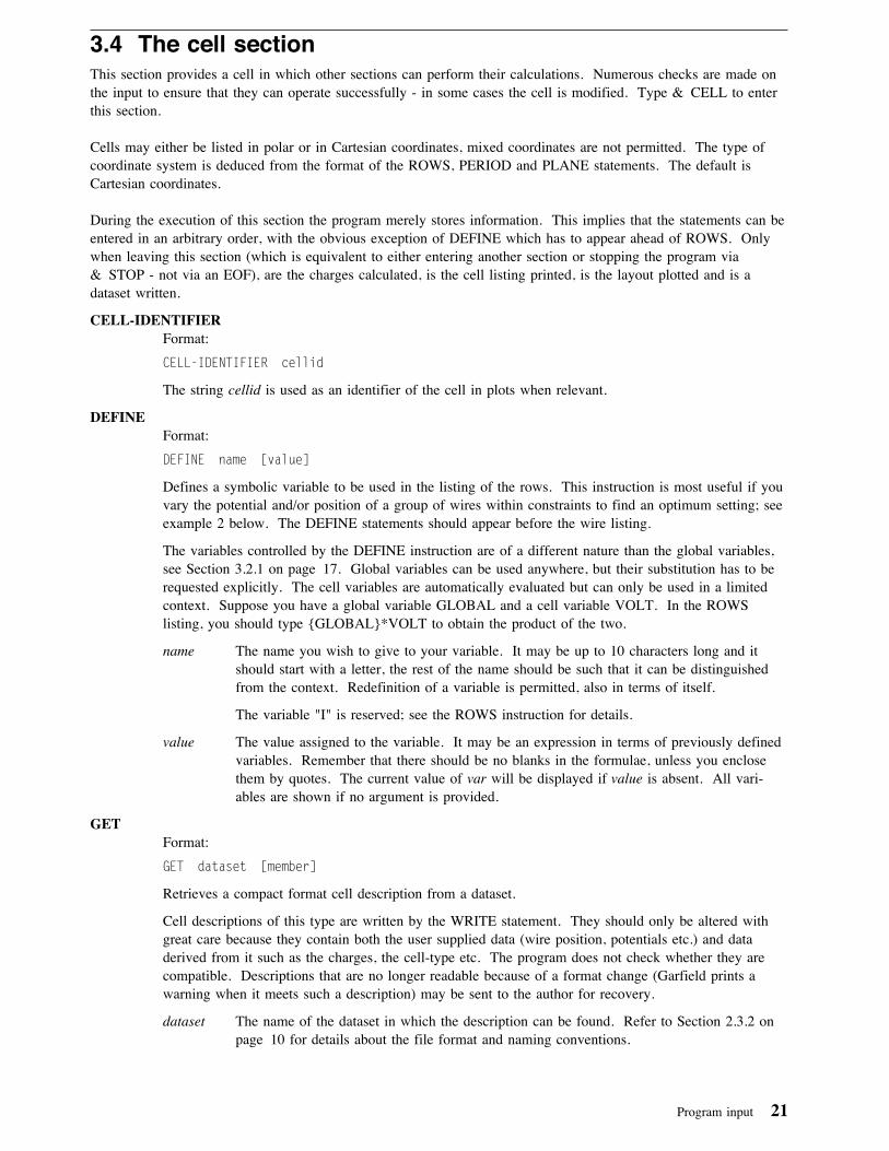
3.4 The cell sectionThis section provides a cell in which other sections can perform their calculations. Numerous checks are made onthe input to ensure that they can operate successfully - in some cases the cell is modified. Type & CELL to enterthis section.

Cells may either be listed in polar or in Cartesian coordinates, mixed coordinates are not permitted. The type ofcoordinate system is deduced from the format of the ROWS, PERIOD and PLANE statements. The default isCartesian coordinates.

During the execution of this section the program merely stores information. This implies that the statements can beentered in an arbitrary order, with the obvious exception of DEFINE which has to appear ahead of ROWS. Onlywhen leaving this section (which is equivalent to either entering another section or stopping the program via& STOP - not via an EOF), are the charges calculated, is the cell listing printed, is the layout plotted and is adataset written.

CELL-IDENTIFIERFormat:

CELL-IDENTIFIER cellid

The string cellid is used as an identifier of the cell in plots when relevant.

DEFINEFormat:

DEFINE name [value]

Defines a symbolic variable to be used in the listing of the rows. This instruction is most useful if youvary the potential and/or position of a group of wires within constraints to find an optimum setting; seeexample 2 below. The DEFINE statements should appear before the wire listing.

The variables controlled by the DEFINE instruction are of a different nature than the global variables,see Section 3.2.1 on page 17. Global variables can be used anywhere, but their substitution has to berequested explicitly. The cell variables are automatically evaluated but can only be used in a limitedcontext. Suppose you have a global variable GLOBAL and a cell variable VOLT. In the ROWSlisting, you should type {GLOBAL}*VOLT to obtain the product of the two.

name The name you wish to give to your variable. It may be up to 10 characters long and itshould start with a letter, the rest of the name should be such that it can be distinguishedfrom the context. Redefinition of a variable is permitted, also in terms of itself.

The variable "I" is reserved; see the ROWS instruction for details.

value The value assigned to the variable. It may be an expression in terms of previously definedvariables. Remember that there should be no blanks in the formulae, unless you enclosethem by quotes. The current value of var will be displayed if value is absent. All vari-ables are shown if no argument is provided.

GETFormat:

GET dataset [member]

Retrieves a compact format cell description from a dataset.

Cell descriptions of this type are written by the WRITE statement. They should only be altered withgreat care because they contain both the user supplied data (wire position, potentials etc.) and dataderived from it such as the charges, the cell-type etc. The program does not check whether they arecompatible. Descriptions that are no longer readable because of a format change (Garfield prints awarning when it meets such a description) may be sent to the author for recovery.

dataset The name of the dataset in which the description can be found. Refer to Section 2.3.2 onpage 10 for details about the file format and naming conventions.

Program input 21

member The member name of the description, a string of up to 8 characters. You may use awildcard for this item: DC*1 will for instance match DC1 and DC-TST-1 but notDC-1-TST. The default is an asterisk, matching every member name. The first member inthe dataset that is a cell description and matches the member name you specify, will beread. The %INDEX command can be used to find out which members have been stored ina given dataset.

OPTIONSFormat:

OPTIONS [NOCELL-PRINT | CELL-PRINT][NOLAYOUT | LAYOUT][NOTISOMETRIC | ISOMETRIC][NOWIRE-MARKERS | WIRE-MARKERS]

Sets a few options controlling the amount of output. The table and the plot are produced when leavingthe section.

CELL-PRINTPrints a table which contains everything the program knows about the cell.

LAYOUTPlots the layout of the cell.

ISOMETRICThe layout plot will not be distorted if this option is active.

WIRE-MARKERSWires are by default plotted circles with the size of the wire. You may prefer to have themrepresented by markers of different kinds. This can be achieved by choosing theWIRE-MARKERS option. The markers can be chosen via the !REPRESENT graphicscommand.

When the WIRE-MARKERS option is on, the wires are not labeled by their code letter inthe LAYOUT plot.

Technical note: wires are by default plotted as hollow fill-area objects so that they can bepointed at in some commands like GRAPHICS-INPUT in the drift section. With theWIRE-MARKERS option on, they are plotted as polymarkers.

PERIODFormat:

PERIOD {X|Y|PHI} length

Indicates that the cell should be periodic in x, y or φ, use two of these statements for doubly periodiccells.

X|Y|PHI The direction in which the cell should be periodic. Note that radial symmetry is notallowed.

length The distance after which the cell should repeat itself [in cm or �, no default is supplied].

PLANEFormat:

PLANE {X|Y|R|PHI} coordinate [VOLTAGE potential]

Enters an equipotential plane. The planes may be at constant x, y or φ, but circular planes at constant rare also allowed. One may not place a wire at the center of a circular plane, see the TUBE statementfor an alternative.

X|Y|R|PHIShould be obvious.


coordinateThe location of the plane, in cm if the plane is at constant x, y or r and in degrees if theplane is at a constant angle to the x-axis [default is 0, which is not acceptable for circularplanes].

potentialThe voltage of the plane [default: 0 V i.e. a grounded plane].

RESETFormat:

RESET [COORDINATES] [DEFINITIONS] [DIELECTRICA] [PERIODICITIES] [PLANE]

[ROWS or WIRES]

(Only in interactive mode) resets selectively the cell data entered so far. All data are erased if thearguments are omitted. The COORDINATES keyword is used to change from polar to Cartesian coor-dinates or vice versa.

ROWSFormat:

ROWS [CARTESIAN | POLAR]code n diameter x_start y_start [V_start [dx [dy [dV]]]]code n diameter x_start y_start [V_start [dx [dy [dV]]]]...(blank line)

The lines following the ROWS statement should be a listing of the wire rows. A row is a set ofregularly spaced wires; examples are a series of equidistant wires, a spiral a parabola etc. A blank linesignals the end of the list.

The cell is by default assumed to be entered in Cartesian coordinates; specifying POLAR overrides thischoice. Alternatively, you may first enter a plane or a periodicity, the format of which fixes the coordi-nate system. All elements of the cell (wires, planes and periodicities) must be entered in the samecoordinate system.

A wire may not be positioned at the origin if polar coordinates are being used. This case can be addedto the program if there is sufficient interest.

Make sure that all the wires are on one and the same side of the equipotential planes, if they arepresent in your chamber. The program counts the number of wires on either side of each plane andremoves those that form the minority. The wires are moved into the basic cell (coordinate rangingfrom -s/2 to s/2, where s is the period) if the cell is periodic. This should not affect the validity of theresults but it is worth noting since the copy of the wire in the basic cell plays a privileged role.

code One-letter code (all upper-case letters are acceptable) for the type of the wires. The 'S'wires are initially considered to be sense wires, i.e. the wires for which signals and x(t)-relations are calculated, from which drift-lines start in certain plots etc. You may at anytime select a different set of sense wires. Convenient codes can be very useful, choosethem carefully ! You may, if you wish, label the wires with more than one character butonly the first will be remembered.

n Number of wires in the row [default is 1].

diameter The diameter (and not the radius !) of all the wires in the row [default: 0.010 cm]. If thediameter varies within the row, you may resort to using the loop-variable described below.

x_start x- or r-coordinate of the first wire in the row [in cm].

y_start y- or φ-coordinate of the first wire in the row [in cm or degrees].

V_start Voltage of the first wire in the row [default: 0.0 V].

Program input 23

dx Increment of the x- or r-coordinate [default: 0.0 cm]. The loop-variable described belowoffers considerably greater flexibility than increments.

dy Increment of the y- or φ-coordinate [default: 0.0 cm or �]. The loop-variable describedbelow offers considerably greater flexibility than increments.

dV Increment of the voltage [default: 0.0 V]. The loop-variable described below offers consid-erably greater flexibility than increments.

n, diameter, x_start, y_start, V_start, dx, dy and dv are allowed to be expressions in terms of symbolicparameters defined by DEFINE earlier on in the same section.

In addition to the variables you define via DEFINE, there is one variable the program defines for you:the loop-variable. This variable, called I, takes on the values 0 for the first wire in the row, 1 for thesecond ... and n-1 for the last. A typical use of this would be the construction of electrodes such asparabolas and ellipses (see the third example below). The approximation for these electrodes is verysimilar to that obtained with finite element methods but with the advantage that the sense wires arehandled accurately. The loop-variable may only be used in d, x_start, y_start and V_start. When youuse the loop-variable, you may still provide increments but they should not depend on I. Clearly, theloop-variable renders the increments obsolete: substitute x_start+I*dx for x_start and drop dx (andsimilarly for y and V). Refer to Section 4.5 on page 116 for details about the formulae.

TUBEFormat:

TUBE RADIUS r [VOLTAGE v] [EDGES n]

Defines a tube surrounding the wires. The tube is by default circular, but can also be triangular, square,hexagonal etc. A tube is in many respects like a circular plane, with the following exceptions however:

• the coordinate system used for input and output is Cartesian, not polar;

• one is allowed to put a wire at the center of a tube, which is not allowed for circular planes;

• one can only have one tube per cell.

A tube can be combined with a φ-periodicity, but not with periodicities in x or y, nor with planes.

r The radius of the tube, for non-circular tubes r is the distance between the center and oneof the corners.

v The potential at which the tube is placed.

[By default 0 V.]

n The number of corners of the tube. Instead of EDGES=3 one can also type TRIANGLE,and similarly for SQUARE, PENTAGON, HEXAGON, HEPTAGON and OCTAGON. Toobtain a cylindrical tube, one can specify CIRCLE, CYLINDER or EDGES=0.

[By default, the tube is cylindrical.]

WRITEFormat:

WRITE DATASET dataset [member] [REMARK remark]

Writes, while leaving the cell section, all available cell data on a dataset. This instruction, which mayappear anywhere in the cell section, can be very efficient if recalculating the wire charges takes a lot oftime. Otherwise the < instruction is probably more flexible. The dataset may exist prior to programexecution, in which case the data will be appended and a member name may be required to retrieve thedata. The DATASET and REMARK keywords may be omitted, provided the order of the arguments isrespected: e.g. member has to be specified if you wish to have a remark.

dataset The dataset you would like to write the description on. Refer to Section 2.3.2 on page 10for details about the file format and naming conventions.


member An 8 character code, to be used when more than one cell description is stored in thedataset. All characters are permitted, case is only preserved if the member name isenclosed by double quotes.

remark An optional remark which could help in recognising the data.

Z-RANGEFormat:

Z-RANGE zmin zmax

Establishes the z-dimensions of the cell. This information is used as default z-component of the AREAin the drift section. Use of this statement is optional ans is only meaningful if you have a magneticfield.

Example 1, a simple valid cell section:

& CELLOPTIONS CELL-PRINT LAYOUTWRITE "garfield/cells/DC1"ROWSS 5 * �.� �.� �.� �.4

PLANE X=-2, V=-7��PLANE X=+2, V=-7��

This cell (Cartesian coordinates are used) has 5 sense wires (they are all at 0 V, have a diameter of 100 μm and areon the y-axis spaced by 4 mm), 2 equipotential planes (one at x = −2 cm and one at x = +2 cm, both at −7000 V)and the cell is not periodic. A layout plot will be made, a description of the cell will be printed and the celldescription will be written to the external dataset garfield/cells/DC1 (Unix file naming).

Example 2, demonstrating the use of DEFINE:

& CELLdefine V_high -5��define V_low -2��DEF VSENSE �ROWSS 4 * � � VSENSE � 1P 2 * -1 � V_high 2P 2 * -1 1 V_low+(V_high-V_low)/3 2P 2 * -1 2 V_low+(V_high-V_low)/5 2P 2 * -1 3 V_low 2

WRITE dataset 'CELL LIB' RESISTOR ...remark "Vhigh=-5�� V, Vlow=-2�� V"

The potentials of the P wires are derived from a resistor chain in this example. All potentials on the P wires areautomatically corrected when V_low and V_high are changed. The description of the cell is written to the CMSdataset CELL LIB on the A disk of the user running the program. Note the use of single and double quotes in theWRITE statement, CMS requires that dataset names are in upper-case and hence single quotes are used for thedataset. The double quotes around the remark prevent the conversion to upper-case of the string. Example 3, theloop-variable:

& CELLcell-id "Circle"define n_wire 5�rowsp n_wire * cos(2*pi*i/n_wire) sin(2*pi*i/n_wire) -1��s * * � � +5��

Or how to make a circle ... if you like spirals, try the next one:

Program input 25

& CELLcell-id "Spiral"define n 5�rowsp n * (1+i/2�)*cos(3*pi*i/n) (1+i/2�)*sin(3*pi*i/n) -1��s * * � � +5��


3.5 The magnetic field sectionThis program does not allow for complicated magnetic field patterns, unless a routine (called BFIELD, see Section6.3 on page 129) is replaced. Simple linear magnetic fields may however be entered from the input and the dis-tortion due to the wires will be taken into account if requested. The influence of the B-field on the behaviour ofthe electrons and ions is described in Section 4.3 on page 110.

WARNING: The calculated Lorentz angle may differ considerably from the experimental values, at least athigh B. Apparently no simple formula matches the data for all B and ad hoc corrections [1] may have to beintroduced in routine DLCVEL.

The header line for this section is & MAGNETIC and the following are valid instructions:

COMPONENTSFormat:

COMPONENTS [bx by bz] [GAUSS | TESLA]

Sets the components of the magnetic field.

bx by bz are the 3 components of the magnetic field. [default: 0 G for all three components, i.e.switching the field off; see below for the units.]

GAUSS Use this when the field is entered in Gauss, internal units of 100 Gauss are assumed if nounit is given.

TESLA Use this when the field is entered in Tesla, internal units of 0.01 Tesla are assumed if nounit is given.

OPTIONSNo specific options for this section.

SUSCEPTIBILITYFormat:

SUSCEPTIBILITY [wires gas]

May be used to set the magnetic susceptibilities of the wires and the gas [any unit: only the ratiomatters, defaults are 1 and 0 which gives an α of 1, probably the only value of α you will ever need;see also Section 4.1.11 on page 105].

Example:

& MAGNETICcomponents � � 3 Gauss

Program input 27

3.6 The gas sectionThe purpose of the gas section is to enter a description of the gas that you wish to have in your chamber. Thereare several ways to enter the gas description:

• For some built-in gasses and gas mixtures it is enough to type the name of the gas. This is for instance thecase for Argon-Ethane 50/50.

• You can also ask the program to compute the drift velocity and diffusion for mixtures of gasses, using built-intables of the elastic cross section and the fraction of the energy lost by electrons during collisions with the gas.See Section 3.6.1 for details.

• In case you measured e.g. the drift velocity, you may prefer to enter your experimental data directly. This canbe done via the TABLE instruction described below. Details on this can be found in Section 3.6.2 on page 30.

The header line to enter this section is & GAS.

All data, whatever their origin, should apply to the zero magnetic field situation.

3.6.1 Built-in gassesThe following 2 lines are sufficient to use CO2.

& GASCO2

Similar instructions exist for the other built-in pure gasses and commonly used gas mixtures:

ARGON-20-ETHANE-80Loads a mixture of 20 % argon and 80 % ethane.



ARGON-73-METHAN-20-PROPANOL-7Loads a mixture of 73 % argon, 20 % methane with 7 % propanol.

CO2Loads pure CO2.

CO2-80-ETHANE-20Loads a mixture of 80 % CO2 and 20 % ethane.

CO2-90-ETHANE-10Loads a mixture of 90 % CO2 and 10 % ethane.

CO2-90-ISOBUTANE-10Loads a mixture of 90 % CO2 and 10 % isobutane.

ETHANELoads pure ethane.

ISOBUTANELoads pure isobutane.

METHANELoads pure methane.

The origin of the data is quoted in the program listing, the quality is not guaranteed by the author of Garfield. Theoptions GAS-PLOT and GAS-PRINT may be used to verify that the data are adequate.

MIXFormat:


MIX [ ARGON frac ] [ HELIUM frac ] [ METHANE frac ] [ ETHANE frac ] [ NEON frac ] [ NITROGEN frac ] [ ISOBUTANE frac ] [ XENON frac ] [ CO2 frac ] [ METHYLAL frac ]

[ KRYPTON frac ] [ AMMONIA frac ]

[ MINIMUM-ENERGY emin ][ MAXIMUM-ENERGY emax ][ STEPSIZE-ENERGY estep ]

[ CRITICAL-F�-FRACTION frcrit ]

[ RANGE epmin epmax ] [ N n ][ LINEAR-E/P-SCALE | LOGARITHMIC-E/P-SCALE ]

[ PLOT-F� | NOPLOT-F� ][ PLOT-ENERGY-LOSS | NOPLOT-ENERGY-LOSS ][ PLOT-CROSS-SECTION | NOPLOT-CROSS-SECTION ][ PLOT-PATH | NOPLOT-PATH ]

[ PRINT-TABLES | NOPRINT-TABLES ]

Garfield computes the drift velocity and diffusion coefficient of gas mixtures following the treatment byG. Schultz and J.Gresser [2], using cross section and energy loss data provided by Fabio Sauli andAnna Peisert [3], from the paper cited above and from WIRCHA [4]. Although reasonably accurate forlow E/p, the absence of a treatment of ionisation makes the results unuseable for large E/p. Theprogram issues a warning if ionisation is likely to affect the results. One should note also that severalother programs exist that do similar calculations, e.g. WIRCHA [4].

fracThe fraction of the mixture taken up by the gas. The fractions do not necessarily have toadd up to 1.

[Each fraction is 0 by default.]

eminThe lowest point of the electron energy range in the cross section, energy loss, mean freepath and F0 plots.

The value of this parameter has no impact on the drift velocity and diffusion calculations.

[By default 0.01 eV.]

emaxThe largest electron energy which is considered during the computations of F0, the driftvelocity and the diffusion. This is also the largest electron energy shown in the crosssection, energy loss, mean free path and F0 plots.

This parameter should be chosen sufficiently large. Results may be inaccurate results andthe effect of ionisation may go undetected if this parameter is too small. The only negativeresult of choosing this parameter too large is an increased CPU time consumption.

[By default 25 eV.]

estepThe largest step size allowed during integration. One should keep in mind that integrationin each step is done using a 6-point Gauss technique and that the steps never bridge achange-over between two parametrisations.

[By default 0.5 eV.]

frcritGarfield checks for each point of E/p that not more than a fraction frcrit of F0 exceeds thelowest ionisation level of any of the gas components.

[By default 0.01, i.e. 1 %.]

Program input 29

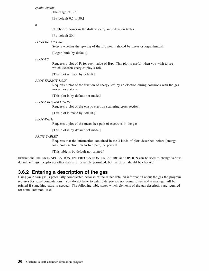
epmin, epmaxThe range of E/p.

[By default 0.5 to 50.]

nNumber of points in the drift velocity and diffusion tables.

[By default 20.]

LOG/LINEAR scaleSelects whether the spacing of the E/p points should be linear or logarithmical.

[Logarithmic by default.]

PLOT-F0Requests a plot of F0 for each value of E/p. This plot is useful when you wish to seewhich electron energies play a role.

[This plot is made by default.]

PLOT-ENERGY-LOSSRequests a plot of the fraction of energy lost by an electron during collisions with the gasmolecules / atoms.

[This plot is by default not made.]

PLOT-CROSS-SECTIONRequests a plot of the elastic electron scattering cross section.

[This plot is made by default.]

PLOT-PATHRequests a plot of the mean free path of electrons in the gas.

[This plot is by default not made.]

PRINT-TABLESRequests that the information contained in the 3 kinds of plots described before (energyloss, cross section, mean free path) be printed.

[This table is by default not printed.]

Instructions like EXTRAPOLATION, INTERPOLATION, PRESSURE and OPTION can be used to change variousdefault settings. Replacing other data is in principle permitted, but the effect should be checked.

3.6.2 Entering a description of the gasUsing your own gas is potentially complicated because of the rather detailed information about the gas the programrequires for some computations. You do not have to enter data you are not going to use and a message will beprinted if something extra is needed. The following table states which elements of the gas description are requiredfor some common tasks:


It is often a good idea to store the gas description in a dataset to be input either via < file_name or via GETfile_name.

CLUSTERFirst format:

CLUSTER

P�, P1, ......... Pn – 1, Pn(blank line)

If the primary cluster-size distribution has been measured, it is of course preferable to use it instead ofthe Landau approximation. The probabilities for the various cluster-sizes should be enumerated on oneor more lines following this instruction. The first number is assumed to be the chance that a cluster hasa size of 0 (!). The probabilities do not have to add up to 1. A blank line is interpreted as the end ofthe list.

Second format:

CLUSTER distribution [N n]

To be used if a parametrisation of the cluster-size distribution is known.

distributionShould be a function of the symbolic parameter N, the cluster size. The function need notbe normalised.

nThe number of data-points. The maximum cluster-size which can be generated will be n-1.[default: 20]

EXTRAPOLATIONSFormat:

EXTRAPOLATIONS[LOW-DRIFT-VELOCITY { LINEAR | CONSTANT | EXPONENTIAL } ][LOW-ION-MOBILITY {...} ][LOW-DIFFUSION-COEFFICIENT {...} ][LOW-TOWNSEND-COEFFICIENT {...} ][LOW-ATTACHMENT-COEFFICIENT {...} ][HIGH-DRIFT-VELOCITY {...} ][HIGH-ION-MOBILITY {...} ][HIGH-DIFFUSION-COEFFICIENT {...} ][HIGH-TOWNSEND-COEFFICIENT {...} ][HIGH-ATTACHMENT-COEFFICIENT {...} ]

Table 2. Use of gas data. The table shows for some common tasks which elements of the gas description are required.

task ve μion σdiffusion αTownsend βatt clusterdata

field calculations no no no no no no

drifting electrons yes no optional optional no no

drifting ions no yes optional optional no no

x(t)-relations yes no optional no no no

arrival time yes no yes no yes yes

signals yes yes optional optional yes yes

Note: Users familiar with the interiors of the program may note that the columns in the table correspond withthe GASOK bits.

Program input 31

This instruction provides some flexibility in the way the program extrapolates to smaller and larger E/pvalues than those found in the table. EXTRAPOLATIONS will overrule the settings for built-in gassesand for gasses read via GET statements, provided the EXTRAPOLATIONS statement follows thecommand via which the gas data were obtained.

LINEARA linear extrapolation based on the first and last two data-points, which should be chosenjudiciously. The program warns if the extrapolation is negative beyond some E/p and theinterpolation routine will return 0 from that point onwards.

EXPONENTIALAn exponential extrapolation taking only the first and last two data-points into consider-ation. They should be chosen very carefully, especially if the table does not extend to verysmall and large E/p (in which case this extrapolation method may prove disastrous, eventhough it has been protected against overflow).

CONSTANTThe constant method sets the corresponding item to the value of the first and last data-pointfound in the table.

GAS-IDENTIFIERFormat:

GAS-IDENTIFIER gasid

The string gasid is used as an identifier for the gas. It will appear in the upper left hand corner of theplots when relevant.

GETFormat:

GET dataset [member]

Retrieves a compact format gas description from a dataset. Gas descriptions of this type are written bythe WRITE statement.

They should only be altered with great care because they contain both the user-supplied data (tables andparameters) and data derived from it (interpolation coefficients, cluster-size distribution). The programdoes not check whether they are compatible. Descriptions that are no longer readable because of aformat change (Garfield prints a warning when it meets such a description) may be sent to the authorfor recovery.

dataset The name of the dataset in which the description can be found. Refer to Section 2.3.2 onpage 10 for details about the file format and naming conventions.

member The member name of the description, a string of up to 8 characters. You may use awildcard for this item: AR*80 will for instance match AR20ET80 or AR80 but notAR80ET20. The default is an asterisk, matching every member name. The first member inthe dataset that is a gas description and matches the member name you specify, will beread. The %INDEX command can be used to find out which members have been stored ina given dataset.

INTERPOLATIONFormat:

INTERPOLATION[DRIFT-VELOCITY { SPLINES | NEWTON order } ][ION-MOBILITY {...} ][DIFFUSION-COEFFICIENT {...} ][TOWNSEND-COEFFICIENT {...} ][ATTACHMENT-COEFFICIENT {...} ]

This statement permits you to alter the interpolation scheme used to compute the drift-velocity, thediffusion, the attachment coefficient and the Townsend coefficient for E/p points that are within therange of the table.


SPLINESSplines have continuity properties that make them attractive for use by integration routines,such as those used for calculation drift-lines. Cubic splines do however have a tendency tooscillate. [By default, all tables except those for some built-in gasses are interpolated usingcubic splines.]

NEWTONNewton polynomial interpolation is less affected by oscillations provided the order of theinterpolating points is chosen sufficiently small. The result is not as smooth as splineshowever.

orderThe order of the interpolating polynomial; 1 and 2 are recommended values. Values abovethe number of table entries - 1 or above 10 are not permitted, neither are negative numbers.[Default: 2].

OPTIONSFormat:

OPTIONS [NOGAS-PLOT | GAS-PLOT][NOGAS-PRINT | GAS-PRINT]

There are a few options for this section:

GAS-PLOTEnables plotting the curves of ve, vion, σdiffusion, αTownsend and βatt vs log(E/p), provided thedata are available. Samples of this type of plot are shown in Figure 1 on page 34,Figure 2 on page 34 and Figure 3 on page 34.

GAS-PRINTEnables printing of all available gas data.

Program input 33

Figure 1. Drift-velocity in CO2 Figure 2. Diffusion coefficient of CO2

Figure 3. Townsend coefficient of CO2

The plots on this page were produced with the fol-lowing set of commands:

& GASopt gas-plotCO2


PARAMETERSFormat:

PARAMETERS [A a Z z E-MOST-PROBABLE e_mp E-PAIR e_pair RHO ρ] [MEAN n_mean]

This statement enters some parameters mainly used for the signal simulation. A, Z,E-MOST-PROBABLE, RHO and E-PAIR may be omitted if you enter the cluster-size distributiondirectly via CLUSTER, (see also Section 4.4.1.2 on page 113). MEAN is required for all signal simu-lations. The MOBILITY is needed for ion-drifting and hence amongst others for signals.

a Atomic number of the gas.

z Nuclear charge of the gas atoms or molecules.

e_mp Most probable energy loss per cm (at density ρ) [eV/cm].

e_pair Energy needed to form one electron ion pair [eV].

n_mean Average number of clusters per cm.

ρ Density of the gas [g/cm3].

PRESSUREFormat:

PRESSURE p

Changes the gas pressure to p [in torr, default is 760 torr]. This instruction can be used to change thepressure of gasses read from a dataset (GET) or from a routine (like CO2).

RESETClears the gas-data.

TABLEFormat:

TABLE [E/p] [DRIFT-VELOCITY [fe] ] [ION-MOBILITY [fion] ] [DIFFUSION-COEFFICIENT [fσ] ] [TOWNSEND-COEFFICIENT [fa] ] [ATTACHMENT-COEFFICIENT [fb] ]

[RANGE ep_min ep_max] [N n](at least 3 lines of tabulated items)(blank line)

This instruction enters the drift velocity, the diffusion coefficient, the Townsend coefficient and theattachment coefficient. You don't have to enter all of them; error messages are printed if some data areabsent. The order in which the quantities are listed may be chosen freely. The next examples illustratethe various ways to use this statement.

E/pRepresents the field-strength [in V/cm] over the pressure [in torr] in the table. It cannot bea function. The values should be in strictly increasing order and all be > 0. E/p must bepresent if at least one of the items is tabulated and E/p may be used to set the ordinates forinterpolated functions if logarithmic spacing is not convenient.

DRIFT-VELOCITYMake sure that ve > 0 [in cm/μsec].

ION-MOBILITYMake sure that vion > 0 [in cm2/Vμsec].

Program input 35

DIFFUSION-COEFFICIENTMake sure that σdiffusion ≥ 0, [in cm for 1 cm of drift].

TOWNSEND-COEFFICIENTenter αTownsend/p, not α, in view of the pressure scaling that will be applied. [in 1 / (cmtorr)].

ATTACHMENT-COEFFICIENTenter βatt/p, not β, in view of the pressure scaling that will be applied. [in 1 / (cm torr)].

fe, fion, fσ, fαFunctions for the drift velocity, the diffusion coefficient and the Townsend and attachmentcoefficients divided by the pressure. EP should be used in the functions for E/p. You may,if you wish, use the symbolic variables BOLTZMANN (kB = 1.38066 × 10−23J/K) andECHARGE (qe = 1.6021892 × 10−19C) in the expressions. All functions will be sampled ateither the E/p values listed in the table or at logarithmically equidistant points. The datathus obtained are interpolated during the calculations, like tabulated data. Refer to Section4.5 on page 116 for details about the syntax of the formulae.

ep_minLowest value of E/p for which the formulae are valid [default is 0.01]. The value at thispoint plays a major role if drift velocities, diffusion coefficients, Townsend coefficients orattachment coefficients for lower E/p are required. The range is optional and is only takeninto account if no quantity is tabulated.

ep_maxLargest value of E/p for which the formulae are valid [default is 100]. Extrapolated valueswill be used if data for E/p > ep_max are required. The range is optional and is only takeninto account if no quantity is tabulated.

nNumber of points the table will contain [default is 20]. This parameter is only taken intoaccount if no quantity is tabulated.

tabulated itemsEach input lines should contain those entries specified on the TABLE line that were not setequal to a function, in that order. A minimum of three lines is required, a blank linesignals the end of the list. The last few points determine the extrapolation (see EXTRAPO-LATE) and should therefore be chosen with care. Preferably, some points at high E/p (say50 kV/cm torr) should be included.

TEMPERATUREFormat:

TEMPERATURE t

Changes the gas temperature to t The gas temperature is used only for the computation of the driftvelocity and the diffusion coefficient in gas mixtures (MIX).

[in K, default is 300 K].

WRITEFormat:

WRITE DATASET dataset [member] [REMARK remark]

Stores the gas data in compact format in member member of library dataset. A remark may be addedfor easier reference. A member is needed for retrieval if more than one gas description is stored in thedataset. The DATASET and REMARK keywords may be omitted, provided the order of the argumentsis respected: e.g. member has to be specified if you wish to have a remark. Refer to Section 2.3.2 onpage 10 for details about the file format and naming conventions.

Examples:

1. Tabulating each of the items


Tell the program on the TABLE line what information your table contains and use the subsequent lines to enterthe data. The default contents is E/p, ve and σdiff; you don't have to supply arguments to TABLE if that is allyou need. E/p must, of course, be one of the items.

Example:

TABLE E/P DRIFT DIFFUSION TOWNSEND 1 2 3 4 2 5 6 7 3 8 9 1�

* Note the blank line !

2. Tabulating some quantities, using functions for others

Here you should still supply E/p because the E/p value for the functions will be taken from this column;RANGE and N are ignored. Those quantities which will not be listed in the table, should be equated to someexpression.

Example (Thermal limit for the diffusion assuming room temperature and atmospheric pressure (290 K, 760torr):

TABLE E/p DRIFT-VELOCITY ... DIFFUSION=SQRT((2*Boltzmann*29�)/(Echarge*Ep*76�)) 1 2 2 3 3 4

* Note the blank line

3. Using only functions, logarithmic spacing

RANGE and N should be specified (unless you accept the defaults), E/p should not. All quantities must befollowed by an expression. Clearly, no table is needed.

Example (simple parametrisation of α/p for CO2):

table drift-velocity=EP, ...Townsend-coefficient=2�*exp(-466/EP), ...range: 1 1��, n=1�

4. If you don't like logarithmic spacing ...

Consider providing E/p in the table, the RANGE and N will then be ignored.

Example:

TABLE DRIFT=2+LOG(EP) DIFFUSION=EP+2 E/P123

* Note the blank line !

5. Some cluster data

CO2cluster� 1 1

Here CO2 is loaded and the cluster size distribution is then overwritten. The effect can be verified by meansof the CHECK CLUSTER instruction in the signal section.

6. Selecting an interpolation method

Program input 37

& GAStable e/p drift-velocity1 12 13 14 35 36 3

interpolation drift-velocity newton 1opt gas-plot

The drift-velocity has a step in this (artificial) example. Splines will oscillate around such a jump and it istherefore preferable to use linear interpolation.

7. A complete gas section (CO2)

& GAS write dataset='GAS DATA' CO2, remark="Standard CO2" table�.15 �.�8 �.�21��.2� �.1� �.�18��.3� �.15 �.�15��.4� �.2� �.�125�.5� �.25 �.�115�.6� �.3� �.�1�5�.7� �.36 �.�1��.8� �.4� �.��92�.9� �.46 �.��9�1.�� .5� �.��881.5� �.76 �.��782.�� 1.1� �.��743.�� 1.7� �.��724.�� 3.�� .��8�5.�� 5.�� .��966.�� 6.8� �.�1157.�� 8.1� �.�13�8.�� 9.�� .�15�

9.�� 1�.�� .�165 1�.�� 11.�� .�18� 15.�� 13.5� �.�2�� 2�.�� 13.5� �.�2�� 3�.�� 12.5� �.�2�� 4�.�� 14.�� .�2�� 5�.�� 17.�� .�2�� 6�.�� 2�.�� .�2�� 7�.�� 23.�� .�2�� 8�.�� 27.�� .�2�� 9�.�� 3�.�� .�2��1��.�� 33.�� .�2��

para A=22.�, Z=44.�, rho=�.��19, mean=31.�, E-m-prob=3�1�.�para E-pair 33.� mobil �.11E-�5pressure 76�.�

option gas-plot gas-printgas-id "This is normal CO2."


3.7 The optimisation sectionThis section should assist in finding potential settings which satisfy some common requirements such as producingas homogeneous a field-strength or as straight equal-potential contours as possible. Typically, one would startselecting the wires of which one wishes to vary the potentials. Next one could vary the potentials in variousdirections. The potential settings can be saved and restored at any moment. Subsequent sections will see thesettings that are in effect when this section is left.

This section also offers some tools to modify existing cells.

The header line to enter this section reads & OPTIMISE.

AREAFormat:

AREA xmin ymin xmax ymax

Refer to the field section for a description of this command.

CHANGE-VOLTAGESFormat:

CHANGE-VOLTAGES WIRE wire VOLTAGE voltage ...

Sets the voltages of one or more wires to the value you specify. You are allowed to change severalvoltages at the time.

wire The number of the wire of which you wish to change the voltage. This number can befound in the printout that results from the CELL-PRINT option in the cell section.

voltage The new voltage of the wire.

DISPLAYDisplays the current settings of the potentials.

FACTORFormat:

FACTOR [GRID | WIRE | TRACK][NOGROUP | GROUP]

[Instruction temporarily withdrawn]

The field at any point in the cell is a linear function of the wire potentials:

V(z) = Vreference + Vplanes(z) + ∑wires

qi φ(z − zi)

= Vreference + Vplanes(z) + ∑wires

(Vj − Vreference − Vplanes(zj)) {∑wires

cij φ(z − zi)}Similar formulae hold for the electric field. The coefficients between braces are purely geometricalconstants. Knowledge of these coefficients eases the task of finding potential settings corresponding toa given field.

GRID | WIRE | TRACKAveraging can take place either over a given area (GRID - the default) or over a previouslydefined track (TRACK) or over the surfaces of the selected wires (WIRE).

GROUP | NOGROUPSpecifies whether the averages should be grouped following the selection by SELECT ornot. Grouping is on by default.

GRIDFormat:

GRID grid_x [grid_y]

Program input 39

Chooses the density of sampling points used by the SET ON GRID instruction. The points form agrid inside the AREA with regular x (or r, note that this implies an exponential spacing in internalcoordinates) and y (or φ) steps. The first parameter, grid_x, is the number of x- (or r-) divisions;grid_y is the number of y- (or φ-) divisions. Instead of specifying the two arguments, you may specifyonly one in which case the value will be used for both x (or r) and y (or φ). Only values between 2and MXGRID (usually 50) are acceptable [default: 25 for both].

OPTIONSRefer to the field section for a description of this command.

POINTSFormat:

POINTS points

Sets the number of sampling points on the TRACK for the SET ON GRID instruction.

RESTOREFormat:

RESTORE [reference_number]

Restores the potential settings identified by reference_number, a number you obtained from the SAVEinstruction. The original settings will be restored if you omit reference_number or give it a value of 1.

SAVESaves the potential settings in a temporary dataset. The program replies with a reference number whichyou'll need to restore the settings later on.

SELECTFormat:

SELECT wire_codes

The potentials of the wires selected by this statement will be varied by the SET instruction. Groupingis important for SET and also for FACTOR if the GROUP option is on. The wire-codes of the wiresthat are to enter a group, should be enclosed by brackets. E.g. (QR) (S) T will place the Q and R wirestogether in one group, all the S wires in another and the T wires will each form a group.

SETFormat:

SET [field_function][TO {AVERAGE | target_function} ]

[WEIGHT weight][ON {GRID | TRACK | WIRE} ]

[DISTANCE norm] [EPSILON e] [ITERATE-LIMIT itermax]

[PRINT | NOPRINT]

This call plays with the potential settings in an attempt to make field_function as equal as possible tothe target_function in the Euclidean norm with position dependent weighting function weight on a set ofsampling points. Only the potentials of the SELECTed wires are touched. The potentials of wiresforming a group are shifted by the same absolute amount. The sampling points can either be located onthe track or on the grid or on the surfaces of the S-wires. In each case, you have the possibility tochoose the density of points.

In a first stage, the covariance matrix between the wire potentials and the field_function-values on thesampling points is established. By means of a Householder inversion, new values for the wire poten-tials are computed that minimise the Euclidean distance between the two functions on the set of sam-pling points. Then, the new covariance matrix is calculated and a new iteration begins. The Euclideandistance between the field and target functions is never allowed to increase, the step may be shortenedto achieve a decrease. Three conditions can cause the iteration to stop:

• the maximum distance between the field function and the target function drops below norm, whichyou are advised to set yourself,


• the sum of the distances-squared varies by less than a fraction ε between two iterations.

The iteration is aborted if

• the difference can not be made smaller by varying the wire potentials because the field_functiondoes not depend on them to a sufficient extent, for any setting encountered during the minimisationprocedure,

• varying the potential of one wire has numerically the same effect on the field_function as varyingthe potential of another, for any setting encountered during the minimisation procedure,

• the user-chosen maximum number of iterations is reached.

The computations differ slightly between IBM scalar and vector compilations; since the algorithm usedin the vector compilations is numerically superior, convergence there tends to be faster. The differencestems from the modest accuracy of single precision reals on this machine.

field_functionA function of the position and the field [default is V]. The symbolic names you may useare X, Y (or R, PHI for cells in polar coordinates), V, EX, EY (or ER, EPHI) and E.

target_functionA function of the coordinates X, Y (or R, PHI) only, which is used as target for the min-imisation procedure.

weightA function of the coordinates X, Y (or R, PHI) only, which is used to weigh the differencebetween target function and current value of the field function. A larger absolute value ofthe weight causes the minimisation procedure to pay more attention to the point. Allweights must be non-zero. [By default 1 for all points.]

AVERAGESpecifies that the average of field_function is to be evaluated with the initial potential set-tings and that the result should be the target value for the field_function on all points of thetrack or the grid.

GRIDRequests that the sampling points form a regular grid of GRID × GRID points inside theAREA. [This is the initial default.]

TRACKRequests that the sampling points are POINT points on the TRACK.

WIRERequests that the surfaces of the 'S' wires are being sampled, irrespective of the current setof SELECTed wires. The thin-wire approximation is used throughout in that the positionalcoordinates in all functions are taken to be the wire-coordinates (except when evaluating theaverage).

normThe value of

maxsampling points

|field_function − target_function|

at which you will allow the iteration procedure to stop [default is 1].

εThe quantity ε is used both to obtain the derivatives needed by the minimising procedureand for one of the stopping criteria mentioned before. A small value, say 10−4, is suitable ifyou're already close to the optimum potential settings. Larger values, up to say 1, are moreadequate if you are far away. Make sure you don't choose ε smaller than about the squareroot of the single precision accuracy of the computer since some of the derivatives involvedin the minimising procedure are effectively second derivatives. [The default is 10−4, whichis the smallest meaningful value on 32 bit computers.]

Program input 41

itermaxThe maximum number of iterations you permit [default: 10].

PRINTRequests printing of summary information for each iteration cycle.

TRACK x_start y_start x_end y_endRefer to the field section for a description of this command.

Example:

& OPTIMISEtrack 1 1 1 3sel (a) (b)set v to average on track, distance=1�, iterate=2, printsavesel (c) (d)set v to average on track, distance=5, iterate=1�, printrestore 2* Define a grouping and run the FACTOR instructionSEL (S) (PR) QFACTOR GRID


3.8 The field sectionThis section allows you to obtain vector electric field plots, potential contours, a printed table of the field compo-nents etc. The header line for this section is & FIELD. The instructions this section recognises are:

AREAFormat:

AREA xmin ymin xmax ymax

This instruction changes the plotting window, you may wish to use it to obtain detailed pictures of onlypart of the cell or to get plots over several periods. Defaults are the previous boundaries, preset to thecell edges.

xmin x- or r-coordinate of the lower left hand corner of the plots [cm].

ymin y- or φ-coordinate of the lower left hand corner of the plots [cm or degrees].

xmax x- or r-coordinate of the upper right hand corner of the plots [cm].

ymax y- or φ-coordinate of the upper right hand corner of the plots [cm or degrees].

CHECKFormat:

CHECK [WIRE] [PLANE] [MAXWELL] [TUBE] [FULL] [BINS bins] [EPSILON-WIRES eps_wire] [EPSILON-MAXWELL eps_Maxwell]

This is actually a debugging instruction, though it may also be of some use if you need the electricfield on the surface of the wires.

WIREPrints the potential and the electric field-strength at the surface of the sense wires (asselected by SELECT) and checks that the charge per unit length the program has calculatedagrees with the charge found by integrating the normal component of the electric fieldaround a wire:

Qε0

= ∫surface

Enormal dσ

The field at the wire surface is obtained by extrapolation using the Neville algorithm inwhich the spacing of the steps is controlled by the parameter eps_wir.

PLANEPrints the potential and the electric field-strength at the surface of the planes.

TUBEPrints the potential and the electric field-strength at the surface of the tube.

MAXWELLWill check that the potential and electric field are consistent i.e. thatdV/dx = − Ex, dV/dy = − Ey and that the Maxwell equations ∇ • E = 0 (outside the wires)and ∇ • B = 0 are satisfied by the field the program has calculated. It produces a lot ofprinted output and 3 (or 4) histograms.

Each of the differentiations mentioned above is done by comparing the potentials at 2points: one at higher and one at lower coordinate than the sampling points. The displace-ment is (for an x-differentiation) of the type ε (1 + |x|) where ε is the parametereps_Maxwell.

FULLSwitches on all three options. ALL is synonymous with FULL.

Program input 43

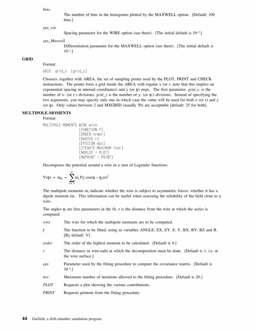
binsThe number of bins in the histograms plotted by the MAXWELL option. [Default: 100bins.]

eps_wirSpacing parameter for the WIRE option (see there). [The initial default is 10−5.]

eps_MaxwellDifferentiation parameter for the MAXWELL option (see there). [The initial default is10−3.]

GRIDFormat:


Chooses, together with AREA, the set of sampling points used by the PLOT, PRINT and CHECKinstructions. The points form a grid inside the AREA with regular x (or r, note that this implies anexponential spacing in internal coordinates) and y (or φ) steps. The first parameter, grid_x, is thenumber of x- (or r-) divisions; grid_y is the number of y- (or φ-) divisions. Instead of specifying thetwo arguments, you may specify only one in which case the value will be used for both x (or r) and y(or φ). Only values between 2 and MXGRID (usually 50) are acceptable [default: 25 for both].

MULTIPOLE-MOMENTSFormat:

MULTIPOLE-MOMENTS WIRE wire [FUNCTION f] [ORDER order] [RADIUS r] [EPSILON eps] [ITERATE-MAXIMUM iter]

[NOPLOT | PLOT][NOPRINT | PRINT]

Decomposes the potential around a wire in a sum of Legendre functions:

V(φ) = m0 + ∑n

i = 1

mi Pi( cos(φ − φi))/ri

The multipole moments mi indicate whether the wire is subject to asymmetric forces, whether it has adipole moment etc. This information can be useful when assessing the reliability of the field close to awire.

The angles φi are free parameters in the fit, r is the distance from the wire at which the series iscomputed.

wire The wire for which the multipole moments are to be computed.

f The function to be fitted, using as variables ANGLE, EX, EY, E, V, BX, BY, BZ and B.[By default: V]

order The order of the highest moment to be calculated. [Default is 4.]

r The distance in wire-radii at which the decomposition must be done. [Default is 1, i.e. atthe wire surface.]

eps Parameter used by the fitting procedure to compute the covariance matrix. [Default is10−4.]

iter Maximum number of iterations allowed to the fitting procedure. [Default is 20.]

PLOT Requests a plot showing the various contributions.

PRINT Requests printout from the fitting procedure.


Figure 4. Example of a SURFACE plot. Figure 5. Example of a HISTOGRAM plot.

Figure 6. Example of a GRAPH plot. Figure 7. Example of a VECTOR plot.

Program input 45

Figure 8. Example of a CONTOUR plot.

The plots on these pages were produced with the fol-lowing set of commands:

& FIELDgrid 5�plot surf hist range � 5��track 1 � 1 5.4area -1.6 �.25 1.6 5.15plot graphgrid 3�plot cont -V label range 18�� 31�� n=13grid 25plot vect

PLOTFormat:

PLOT [CONTOUR [funct1] [RANGE {cmin cmax | AUTOMATIC}] [N ncont]

[LABEL | NOLABEL] ] [GRAPH [funct2] ]

[HISTOGRAM [funct3] [RANGE {hmin hmax | AUTOMATIC}] [BINS n_bins] ] [SURFACE [funct4] [ANGLE φ Θ] ] [VECTOR [funct5 ,funct6] ]

Plots the field in a variety of ways:

• as a set of contours (see Figure 8),

• as a 3-dimensional impression (see Figure 4 on page 45),

• as a histogram (see Figure 5 on page 45),

• as a vector plot (see Figure 7 on page 45),

• as a graph (see Figure 6 on page 45).

The vector, histogram and surface plots are obtained sampling over a grid of GRID × GRID points inthe AREA. Contours are drawn inside the AREA, the GRID parameter determines the density of theinitial searching grid. Graphs use the points on a predefined TRACK which need not be located insidethe AREA. In each PLOT statement, one and only one plot of each type may be requested; CPU timecan be saved if SURFACE, VECTOR and HISTOGRAM are combined because the field will be evalu-ated only once.

cmin cmaxThe lowest and highest function value for which a contour will be plotted. AUTOMATICmeans that cmin and cmax will be set such that the range of the function over the area iscovered and all contours heights are round numbers. [Defaults are the extremes of thepotential in the whole cell if contours of V are requested, 0 and 10000 else. However,automatic adjusting of the range is default and to obtain the settings described before, youhave to specify RANGE * *.]


ncontThe number of contours to be plotted minus 1. [Default is 20.]

If you opt for automatic scaling, the number of contours you see, is sometimes larger thanncont+1. Your value of ncont is used to obtain a rough distance between two contourswhich is rounded downwards to the nearest power of 10 times 1, 2 or 5. The bounds of therange are set equal to multiples of the rounded distance.

LABELRequests labelling of the contours. [On by default, only available from version 2.01onwards.]

hmin hmaxLower and upper bound of the histogram. If you specify AUTOMATIC, the range of thehistogram is set to the interval [x − 3MADx, x + 3MADx] rounded outwards. The firstfew (usually 100) entries serve to compute the mean and MAD. These entries are notnecessarily representative for the whole sample. [Default is automatic scaling.]

n_binsThe number of channels the histogram should have [default is 100].

φ θThe viewing angles used to project the surface plots [in degrees, defaults: 30� for φ and60� for θ].

funct.Functions to be plotted. Variables allowed in the expressions are X, Y, EX, EY, E, V, BX,BY, BZ and B (the latter 4 only if there is a magnetic field). If the cell is described inpolar coordinates, X, Y, EX and EY must be replaced by R, PHI, ER and EPHI. Note thatthere should be no blanks in the expressions. Defaults are V for contours, surface plots andgraphs, E for histograms and (EX,EY) for vector plots.

You may substitute a commercial at @ for any of the functions. You will find yourself inthe algebra editor where you can manually construct an instruction list. See also Section4.5 on page 116 for details about the formulae.

PRINTFormat:

PRINT funct1 [funct2 [funct3 ... ]]

Prints the value of the functions funct1, funct2 ... of the field on a grid of GRID × GRID points in theAREA. Each set of tables contains 4 of the functions. Be careful, this command generates a lot ofoutput (25 pages for GRID=50).

SAMPLEFormat:

SAMPLE x y

Prints the field at (x,y).

SELECTFormat:

SELECT wire-codes

Selects groups of wires for special treatment by, in this section, CHECK WIRE. All wires of which thecode or the wire number (see the table printed in response to the CELL-PRINT option in the cellsection) appears in the argument string, will be considered by CHECK. The concept of wire groups isof no importance here - see the description of this command in other sections for details.

TIMEFormat:

TIME [n]

Times n field evaluations. [Default for n is 1000.]

Program input 47

TRACKFormat:

TRACK x_start y_start x_end y_end

Defines a track to be used by the PLOT GRAPH instruction. Defaults are the previous values, they arenot preset.

x_start x- or r-coordinate of begin point [cm].

y_start y- or φ-coordinate of begin point [cm or degrees].

x_end x- or r-coordinate of end point [cm].

y_end y- or φ-coordinate of end point [cm or degrees].

Example of a valid field section:

& FIELD* First set the options, DEBUG will make the output very bulky !OPTIONS INPUT DEBUG* Define a first large area to be used for the first tableAREA -1 -2 3 2PR EX EY ARCTAN(EY/EX) V* Override the previous area by a smaller oneAREA -�.5 -�.5 -�.4 -�.4PR BX,BY,EX*BY-EY*BXPLOT SURF X**2*SIN(Y) HIST E RANGE 5�� 1��* Get the field at the wire-surface, store it in a dataset> 'GARF OUT'CHECK WIRE* Make sure the rest of the output goes to the screen>


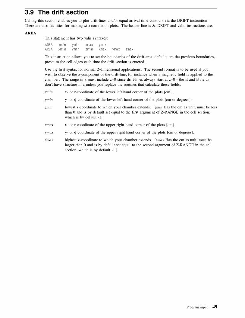
3.9 The drift sectionCalling this section enables you to plot drift-lines and/or equal arrival time contours via the DRIFT instruction.There are also facilities for making x(t) correlation plots. The header line is & DRIFT and valid instructions are:

AREAThis statement has two valis syntaxes:

AREA xmin ymin xmax ymaxAREA xmin ymin zmin xmax ymax zmax

This instruction allows you to set the boundaries of the drift-area, defaults are the previous boundaries,preset to the cell edges each time the drift section is entered.

Use the first syntax for normal 2-dimensional applications. The second format is to be used if youwish to observe the z-component of the drift-line, for instance when a magnetic field is applied to thechamber. The range in z must include z=0 since drift-lines always start at z=0 - the E and B fieldsdon't have structure in z unless you replace the routines that calculate those fields.

xmin x- or r-coordinate of the lower left hand corner of the plots [cm].

ymin y- or φ-coordinate of the lower left hand corner of the plots [cm or degrees].

zmin lowest z-coordinate to which your chamber extends. [zmin Has the cm as unit, must be lessthan 0 and is by default set equal to the first argument of Z-RANGE in the cell section,which is by default -1.]

xmax x- or r-coordinate of the upper right hand corner of the plots [cm].

ymax y- or φ-coordinate of the upper right hand corner of the plots [cm or degrees].

zmax highest z-coordinate to which your chamber extends. [zmax Has the cm as unit, must belarger than 0 and is by default set equal to the second argument of Z-RANGE in the cellsection, which is by default -1.]

Program input 49

Figure 9. Track preparation. The track in this example islocated at -1.5 cm. In a first stage, 15 drift-lineshave been calculated from this track at regulary-intervals. Then, 5 drift-lines have been addedaround the centre to improve the interpolationtable. This plot is made as a result of theDRIFT-PLOT option being on.

Figure 10. Single electron arrival time distribution for onegiven x. The entries in this histogram corre-spond to the times at which the second electronfrom the track shown in Figure 9 reaches thewire in the centre of that plot. A series of suchplots is made if you requestPLOT-EACH-X-SELECTED-ELECTRON.

Figure 11. The inverse interpolation procedure. Thehistogram is the normalised cumulative versionof the one shown in Figure 10. In this example,the second electron is required to have a proba-bility of 0.5 to have reached the wire at the timeshown in Figure 12. This plot is only made ifyou have the DEBUG option switched on.

Figure 12. Overview plot of the arrival time distribution. The solid and dashed lines are the mean arrivaltime of all electrons resp. the second electronsfrom the track. The two dotted lines are thetimes at which any and the second electron have0.5 chance to have arrived. This plot is made ifPLOT-OVERVIEW is selected.


ARRIVAL-TIME-DISTRIBUTIONFormat:

ARRIVAL-TIME-DISTRIBUTION [ELECTRON electron] [THRESHOLD threshold]

[NOAUTOSCALE-TIME-WINDOW | AUTOSCALE-TIME-WINDOW][X-RANGE xmin xmax] [X-STEP-SIZE x_step][Y-RANGE ymin ymax]

[LINES lines] [ANGLE φ][NOSINGLE-CLUSTER | SINGLE-CLUSTER][DATASET dsname [member] ] [REMARK remark]

[BINS bins] [MONTE-CARLO-LOOPS loops][NOKEEP-HISTOGRAMS | KEEP-HISTOGRAMS]

[POLYNOMIAL-ORDER order][NOPLOT-EACH-X-OVERALL | PLOT-EACH-X-OVERALL][NOPLOT-EACH-X-SELECTED-ELECTRON | PLOT-EACH-X-SELECTED-ELECTRON][NOPRINT-EACH-X-OVERALL | PRINT-EACH-X-OVERALL][NOPRINT-EACH-X-SELECTED-ELECTRON | PRINT-EACH-X-SELECTED-ELECTRON][PLOT-OVERVIEW | NOPLOT-OVERVIEW]

The ARRIVAL instruction is a variant of the XT-PLOT instruction. XT-PLOT searches for each x theshortest drift-line from a track, disregarding clustering effects but informing you about the diffusion tobe expected on that shortest drift-line. These calculations are carried out as accurately as possible.

ARRIVAL operates on the same tracks as XT-PLOT does, assuming that your readout triggers at agiven electron count. On each track, the instruction generates clusters a specified number of times,computes the drift-time and generates integrated diffusion coefficients for each electron of each clusterand makes an histogram of the arrival time distribution of the n'th electron to arrive (n is the userspecified parameter electron). The Monte-Carlo nature of the computations sometimes makes theresults less precise than those produced by XT-PLOT but what is computed is closer to what is actuallymeasured. The statistical errors can be made small by choosing proper binning and requesting a largenumber of iterations. Inaccuracies are also introduced by interpolation on the 'prepared track'; the trackpreparation is adopted throughout to make the computations reasonably fast. See Figure 9 on page 50.You can make the interpolation errors small by requesting a large number of table points.

This instruction loops over all SELECTed wires in the current AREA and produces plots and tables foreach of them independently.

electronSpecify here the electron on which you trigger. This is usually a number between 5 and 10but you are allowed to choose any positive integer number you wish. If you are in the tailof the distribution of the number of electrons from the track, you may have to generateclusters more often to obtain reasonable statistics.

Consider using automatic time window scaling if your favourite electron has a sharplypeaked time distribution compared with the overall arrival time distribution.

[Default: 1, remembered across calls.]

thresholdThe program outputs the mean arrival time of the electron'th electron (no histograming usedhere) but also the time at which the electron has arrived with a probability threshold.

This quantity is obtained by reverse interpolation in the cumulative arrival time distributionhistogram using polynomial interpolation of order order.

The parameter threshold ranges from 0 to 1, neither 0 nor 1 are acceptable.

[Default: 0.5, or the median of the distribution, remembered across calls.]

AUTOSCALE-TIME-WINDOWBoth the time distributions of all electrons together and of the selected electrons arehistogramed, see threshold, to estimate the time at which the electron has a certain proba-bility to have arrived. For the overall arrival time distribution, a proper time window isobtained during track preparation. For the selected electron histogram, such a window isnot available and the program uses by default the same window as for the overall timing

Program input 51

histogram. Both the global DEBUG option, which shows details about the reverse interpo-lation procedure (Figure 11 on page 50), and the instruction line optionSHOW-EACH-X-SELECTED-ELECTRON will tell you whether this window is indeedappropriate. If it isn't, you can specify AUTOSCALE-TIME-WINDOW which will choose atime window adapted to the points actually collected. An example of this kind of plot canbe seen in Figure 10 on page 50. [Automatic scaling is the default.]

xmin, xmaxThe range in x to be scanned. This range should be smaller than the x-range of the driftarea.

[Default: the x-range of the current AREA.]

x_stepThe tracks cross the line at constant y through the wire at x-distances... −2 x_step, − x_step, 0, x_step, +2 x_step ... from the wire.

[Default: about 5 % of the x-range of the current AREA.]

ymin, ymaxThe y-range to be scanned. If you are interested only in the first electron, there is no pointin wasting time on the outer edges of the acceptance region of the wire. It is also a wasteof time to have a y-range that extends far beyond the acceptance region of the wire - inaddition, you loose accuracy. On the other hand, if your y-range is too small, you willobtain incorrect results and the program does not warn you if this happens.

[Default: the y-range of the current AREA.]

SINGLE-CLUSTERRequests that only 1 cluster is generated on each track. This may be useful if you wish tosimulate photons.

[Not default, setting remembered across calls.]

linesEach track is first 'prepared': a table of drift-times and integrated diffusion coefficients ismade. This table is subsequently interpolated for each of the clusters. The interpolationimproves if the table is more detailed. Preparing a track is fairly costly in terms of CPUtime but it is generally worthwhile investing in a reasonable high lines value.

[Default: the current setting of LINES.]

φThe angle of the tracks with respect to the y-axis.

[Default: 0 degrees, remembered across calls.]

DATASETRequests the results are written to dataset dsname. You may optionally specify a membername and a remark.

binsThe number of bins in the arrival time distribution histogram.


KEEP-HISTOGRAMSRequests that the arrival time histograms be kept. The histograms are available as globalvariables after command completion. The names of these global variables are printed,usually they are of the type SEL_n and ALL_n with n an integer. Most arithmetic oper-ations can be applied on them, they can be displayed by the PLOT_HISTOGRAM proce-dure etc.

[Default: histograms are not kept.]


loopsThe number of MC cycles.


orderThe order of the interpolating polynomial. Values above 3 are not recommended, you arebetter of if you choose smaller binning and larger statistics. See threshold for more infor-mation.

[Default: 2, parabolic interpolation, remembered across calls.]

PLOT-EACH-X-OVERALLRequests a plot of the arrival time distribution of all electrons for each track.

[Default: off, remembered across calls.]

PLOT-EACH-X-SELECTED-ELECTRONRequests a plot of the arrival time distribution of the selected electron for each track.


PRINT-EACH-X-OVERALLRequests a printout of the arrival time distribution of all electrons for each track. Theprinted version of the histogram provides additional information such as the width of thedistribution.


PRINT-EACH-X-SELECTED-ELECTRONRequests a printout of the arrival time distribution of the selected electron for each track.The printed version of the histogram provides additional information such as the width ofthe distribution.


PLOT-OVERVIEWRequests a plot of the various curves obtained, as a function of x. An overview plot isshown in Figure 12 on page 50.

[Default: on, remembered across calls.]

Figure 13. Example of a DRIFT TRACK plot. Figure 14. The TIME-GRAPH associated with the previousFigure.

Program input 53

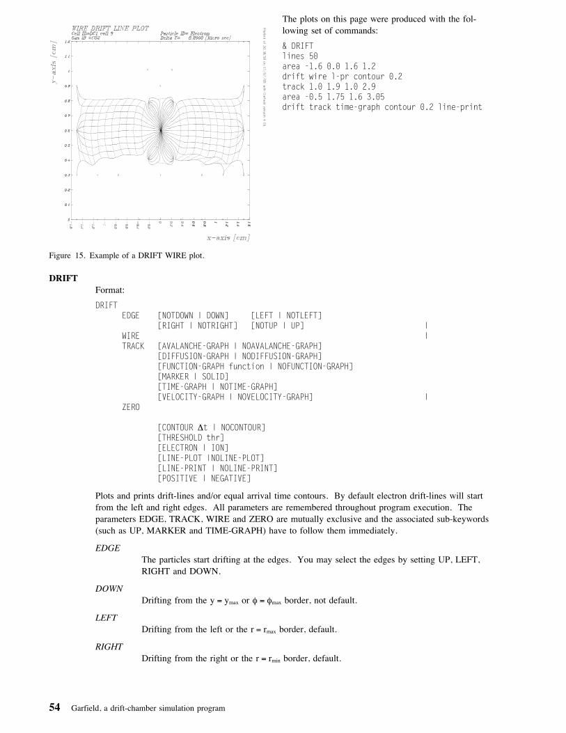
Figure 15. Example of a DRIFT WIRE plot.

The plots on this page were produced with the fol-lowing set of commands:

& DRIFTlines 5�area -1.6 �.� 1.6 1.2drift wire l-pr contour �.2track 1.� 1.9 1.� 2.9area -�.5 1.75 1.6 3.�5drift track time-graph contour �.2 line-print

DRIFTFormat:

DRIFTEDGE [NOTDOWN | DOWN] [LEFT | NOTLEFT]

[RIGHT | NOTRIGHT] [NOTUP | UP] | WIRE |

TRACK [AVALANCHE-GRAPH | NOAVALANCHE-GRAPH][DIFFUSION-GRAPH | NODIFFUSION-GRAPH][FUNCTION-GRAPH function | NOFUNCTION-GRAPH][MARKER | SOLID][TIME-GRAPH | NOTIME-GRAPH][VELOCITY-GRAPH | NOVELOCITY-GRAPH] |

ZERO

[CONTOUR Δt | NOCONTOUR] [THRESHOLD thr]

[ELECTRON | ION] [LINE-PLOT |NOLINE-PLOT]

[LINE-PRINT | NOLINE-PRINT][POSITIVE | NEGATIVE]

Plots and prints drift-lines and/or equal arrival time contours. By default electron drift-lines will startfrom the left and right edges. All parameters are remembered throughout program execution. Theparameters EDGE, TRACK, WIRE and ZERO are mutually exclusive and the associated sub-keywords(such as UP, MARKER and TIME-GRAPH) have to follow them immediately.

EDGEThe particles start drifting at the edges. You may select the edges by setting UP, LEFT,RIGHT and DOWN.

DOWNDrifting from the y = ymax or φ = φmax border, not default.

LEFTDrifting from the left or the r = rmax border, default.

RIGHTDrifting from the right or the r = rmin border, default.


UPDrifting from the y = ymin or φ = φmin border, not default.

TRACKThe particles start drifting from points on a previously defined track. Graphs of the drift-time, the average drift-velocity, the integrated diffusion and the multiplication factor may berequested by specifying one or more of the -GRAPH options. The plot of the drift-linesand equal time contours (see for instance Figure 13 on page 53), can be suppressed byselecting the NOLINE-PLOT and NOCONTOUR options.

TIME-GRAPHProduces a graph of the drift-time for the drift-lines from a track, an example is shown inFigure 14 on page 53.

VELOCITY-GRAPHProduces a graph of the mean drift-velocity for the drift-lines from a track. (Note: thismean is simply the total drift-time divided by a zero'th order estimate of the total length ofthe drift-line.)

DIFFUSION-GRAPHProduces a graph of the integrated diffusion (in μ seconds) for the drift-lines from a track.The routine performing the integration tries to reach full single precision accuracy, in viewof a future upgrade, and is therefore rather slow.

AVALANCHE-GRAPHProduces a graph of the multiplication factor for the drift-lines from a track, integrating theTownsend coefficient. The routine performing the integration tries to reach full single pre-cision accuracy, in view of a future upgrade, and is therefore rather slow.

FUNCTION-GRAPHAllows combining the numbers plotted in the preceding graphs to an almost arbitrary func-tion. The string function should be a function of the following symbolic variables:LENGTH (length of the drift-line), TIME (drift-time), DIFFUSION (integrated diffusioncoefficient) and AVALANCHE (integrated and exponentiated Townsend coefficient).

MARKERThe data in the output of the -GRAPH options are represented by markers, usually anasterisk '*'; the alternative (SOLID) is a continuous line. Track segments leading to dif-ferent wires are always separated by a dashed vertical line, independent of this choice.

WIREThe particles drift backwards from the wires selected as sense wire (by default those with awire-code 'S'). This is the normal mode of drift for ions. This plot is useful with electronsto see where a wire collects charge. Figure 15 on page 54 shows an example of this typeof plot.

ZEROThe particles drift from the zeros of the electric field. The plots obtained this way areuseful in determining the acceptance boundaries of the various wires.

CONTOURSpecifies that equal time contours are to be plotted, Δt is the separation between two equaltime contours [in μsec]. Contours are drawn separately for each wire. The contours arerepresented by broken lines or by asterisks if the line joining two neighbouring points (i)crosses a drift-line or (ii) is longer than a threshold described below. It is perfectly pos-sible to plot equal time contours but no drift-lines.

thrTwo points on an equal time contour are not joined if the distance between them is largerthan a fraction thr of the screen size. [This fraction is initially set to 0.1.]

ELECTRON | IONDrift electrons or ions [preset to electrons].

Program input 55

LINE-PLOTSpecifies that the drift-lines should be plotted.

LINE-PRINTRequests that summary information about the drift-lines be printed.

POSITIVE | NEGATIVEForces the charge of the drifted particle to be positive respectively negative. Do notnormally use this option, the charge is chosen according to the values of the other parame-ters: positive for drift from the wires, negative for drift from the edges and from the track.The option should however be used with DRIFT WIRE in case the selected wires repelelectrons (the program detects this condition but will not modify the charge in order not toconfuse the user). This parameter should, if used, be the last parameter of the statement.

EPSILON εReplaces the absolute integration accuracy by ε. The smaller ε the higher the accuracy, normal valuesare between 10−7 and 10−8. Increasing ε can lower the CPU time consumption considerably. If thesense wires are very thin, a small ε may be needed to avoid that the particles travel around the wire,just outside the trap radius, before they are caught. This shows up very clearly in the DRIFT TRACKTIME-GRAPH plots and the x(t) calculations may fail partly. Another sign that ε is too large, is awobbly drift-line. [Default: 5 × 10−7].

GRAPHICS-INPUTFormat:

GRAPHICS-INPUT[CHOICE-PET chpet] [LOCATOR-PET locpet1 locpet2]

[PICK-PET pickpet] [VALUATOR-PET valpet][CHOICE-DEVICE chdev] [LOCATOR-DEVICE locdev1 locdev2]

[PICK-DEVICE pickdev] [VALUATOR-DEVICE valdev] [WORK-STATION wkid]

(A minimum GKS level of 1b is required.) This is a graphics-menu driven command that enables youto do some simple drift-line calculations without being bothered too much by command syntax.

You may change the AREA and the TRACK by pointing on the screen; most of the other drift-linespecific parameters (to be found in a submenu) can also be modified but their values have to be typed.

Typical things you can ask for are single drift-lines starting at a point you indicate on the screen,drift-lines from the current track and drift-lines from a wire chosen from those visible on the screen.(Drift-lines will also be plotted from the periodic repetitions of a wire, if there are any inside the area.)

This instruction is still experimental and suggestions are welcome. Instructions of this type may beadded for other sections if the need arises.

pet The PET, short for Prompt-Echo Type, controls the method by which graphics input isobtained. For instance, selecting a point may be done using cross hairs, a mouse etc.

You have to specify 2 PET's for locator input since you may wish to use rubber banding toselect the second point of an area, something that clearly does not make sense for the firstpoint. Whenever only one point is required, only the first PET is used.

The PET's you have to enter are largely device dependent.

device By default all input is obtained from device 1, if you have other input devices attached toyour display, you can ask the program to use them instead by specifying a device code.

wkid The identifier of the workstation over which this command should be run.

GRIDFormat:


Sets, together with AREA, the grid for the TABLE instruction. The points form a grid inside theAREA with regular x (or r, note that this implies an exponential spacing in internal coordinates) and y(or φ) steps. The first parameter, grid_x, is the number of x- (or r-) divisions; grid_y is the number of


y- (or φ-) divisions. Instead of specifying the two arguments, you may specify only one in which casethe value will be used for both x (or r) and y (or φ). Only values between 2 and MXGRID (usually 50)are acceptable. [Default: 25]

INTEGRATION-PARAMETERSFormat:

INTEGRATION-PARAMETERS [DIFFUSION-ACCURACY e_diff]

[TOWNSEND-ACCURACY e_a] [DIFFUSION-STACK-DEPTH stack_diff] [TOWNSEND-STACK-DEPTH stack_a]

The diffusion and Townsend integration as used by the DRIFT TRACK and XT-PLOT instruction inthis section and the SIGNAL instruction in the signal section, are performed via an adaptive Simpsonmethod. In case for any drift-line step, the difference between the first and second order estimate differby more than a fraction ε of a crude first order integral, the step is split and integration is attempted forthe two parts independently.

The parameters ε and the maximum stack depth stack, can be chosen changed via this instruction. Theaccuracy parameters are preset to 10−3 and the maximum stack depth to MXSTCK, usually 20.

LINESFormat:

LINES lines

lines Is the number of lines you would like to drift from the surface of each sense wire (DRIFT WIREand XT-PLOT), from each side of the drift-area (DRIFT EDGE) and from the track (DRIFT TRACK).[Default: 20]

LORENTZFormat:

LORENTZ x y

Prints the Lorentz angle (i.e. the angle between the electric field and the drift-speed vector) at the point(x,y).

MINIMISEFormat:

MINIMISE f_min [ON f_curve]

[RANGE t_min t_max] [N n_t] [SELECT f_sel]

[PRINT | NOPRINT] [FUNCTION-PRECISION ef] [POSITIONAL-RESOLUTION ep]

[ELECTRON | ION][NEGATIVE | POSITIVE][DATASET dsn [member] [REMARK remark]]

Searches for the minimum of function the function f_min over the curve f_curve.

f_minThe function to be minimised, f_min, can depend on the variables TIME, LENGTH, DIF-FUSION, AVALANCHE, LOSS, E, B and VELOCITY. The first 5 variables are calcu-lated for a drift line, the last 3 are the local values on the curve of the electric and magneticfield and of the drift velocity.

[This function is by default TIME.]

f_curveThe curve parametrisation should have T as running variable. T assumes values in therange specified with the RANGE keyword. The function f_curve should return two values,

Program input 57

the (x, y) coordinate pair, but is treated as a single input word. The function should there-fore be put between quotes.

[No default provided.]

RANGEThe range of the parameter T of the curve function.

[By default 0 to 1]

f_selA selection function f_sel may optionally be provided. Points on the curve which fail tosatisfy the condition f_sel are not considered by the minimisation procedure. The functionf_sel can depend on the variables TIME, LENGTH, DIFFUSION, AVALANCHE, LOSSand STATUS.

FUNCTION-PRECISIONThe minimising loop is interrupted as soon as the minimum function value changes by lessthan a fraction εf between two iterations.

[Default is 10−4.]

POSITIONAL-RESOLUTIONThe minimising loop is interrupted as soon as the coordinate where the minimum functionvalue was found, changes by less than a fraction εp between two iterations.

[Default is 10−4.]

ELECTRONRequests that minimisation be done for electrons.

[Default.]

IONRequests that minimisation be done for ions.

[Not default.]

POSITIVEForces the charge of the particles to +1.

[Default for ions.]

NEGATIVEForces the charge of the particles to -1.

[Default for electrons.]

PRINTRequests printout at intermediate stages of the minimisation.

[Default.]

DATASETRequests that the results be written to a file.

[Not default.]

The variable STATUS is assigned one of the following values: Hit_x_Wire, Hit_x_Replica, Left_Area,Hit_Plane, Abandoned, Too_Many_Steps, x being the wire type (one letter, upper case). LENGTHstands for the length of the drift line, DIFFUSION for the integrated diffusion coefficient, AVA-LANCHE for the integrated and exponentiated Townsend coefficient and LOSS for the integrated andexponentiated attachment coefficient.

OPTIONSFormat:


OPTIONS[DRIFT-PRINT | NODRIFT-PRINT][DRIFT-PLOT | NODRIFT-PLOT][KEY | NOKEY][CHECK-ATTRACTING-WIRES | CHECK-ALL-WIRES]

The local options for the drift sections are listed below. They are valid also for the signal section withthe exception of KEY.

DRIFT-PLOTEnables plotting of the drift-lines used for XT-PLOT and TABLE. Various other calls willgenerate extra debugging output if this option has been selected. This option has no effecton the DRIFT instruction.

DRIFT-PRINTEnables printing of summarised information about drift-lines used for XT-PLOT andTABLE. Various other calls will generate extra debugging output if this option has beenselected. This option has no effect on the DRIFT instruction.

KEYSpecifies that the drift-time contours should be labeled and that a table of contour heightsshould be plotted. (only in NAG compilations).

CHECK-WIRESWhen the option CHECK-ATTRACTING-WIRES is in effect, the program will only con-sider the wires that attract the particle being drifted as wires the particle can hit. This isadequate except when some of the wires have a clear dipole moment, i.e. wires that attractparticles on one side and repel on the other. The CHECK-ALL-WIRES ensures properdrift-line termination under those circumstances. This option should also be selected whenyou intend to make a DRIFT WIRE plot for slightly repelling wires that have a strongdipole moment.

PLOTFormat:

PLOT [CONTOUR [funct1] [RANGE {cmin cmax | AUTOMATIC}] [N ncont]

[LABEL | NOLABEL] ] [GRAPH [funct2 ] ]

[HISTOGRAM [funct3] [RANGE {hmin hmax | AUTOMATIC}] [BINS n_bins] ] [SURFACE [funct4] [ANGLE φ Θ] ] [VECTOR [funct5 ,funct6] ]

An instruction which is very similar to the PLOT instruction of the field section, except that it plotsinformation related to drift properties. The choice of plots is the same as in the field section: contours,graph, histogram, surface plot and vector plot. The vector, histogram and surface plots are obtainedsampling over a grid of GRID × GRID points in the AREA. Contours are drawn inside the AREA;with a search density controlled by the GRID parameter. Graphs use the points on a predefinedTRACK which need not be located inside the AREA. In each PLOT statement, one and only one plotof each type may be requested; CPU time can be saved if SURFACE, VECTOR and HISTOGRAM arecombined because the field will be evaluated only once.

cmin cmaxThe lowest and highest function value for which a contour will be plotted. AUTOMATICmeans that cmin and cmax will be set such that the range of the function over the area iscovered and all contours heights are round numbers. [Defaults are the extremes of thepotential in the whole cell if contours of V are requested, 0 and 10000 else. However,automatic adjusting of the range is default and to obtain the settings described before, youhave to specify RANGE * *.]

ncontThe number of contours to be plotted minus 1. [Default is 20.]

If you opt for automatic scaling, the number of contours you see, is sometimes larger than

Program input 59

ncont+1. Your value of ncont is used to obtain a rough distance between two contourswhich is rounded downwards to the nearest power of 10 times 1, 2 or 5. The bounds of therange are set equal to multiples of the rounded distance.

LABELRequests labelling of the contours. [On by default, only available from version 2.01onwards.]

hmin hmaxLower and upper bound of the histogram. If you specify AUTOMATIC, the range of thehistogram is set to the interval [x − 3MADx, x + 3MADx] rounded outwards. The firstfew (usually 100) entries serve to compute the mean and MAD. These entries are notnecessarily representative for the whole sample. [Default is automatic scaling.]

n_binsThe number of channels the histogram should have [default is 100].

φ θThe viewing angles used to project the surface plots [in degrees, defaults: 30� for φ and60� for θ].

funct.Functions to be plotted. Variables allowed in the expressions are X, Y (R, PHI for polarcells), EX, EY, E (ER, EPHI for polar cells), BX, BY, BZ, B (only if there is a B-field),VX, VY, VZ, V (local drift velocity, VR, VPHI for polar cells), LORENTZ (local Lorentzangle), TIME (integrated drift time), DIFFUSION (integrated diffusion coefficient), AVA-LANCHE (integrated, exponentiated Townsend coefficient), LOSS (integrated,exponentiated attachment coefficient), STATUS (drift line status cose), P (gas pressure).Note that there should be no blanks in the expressions.

You may substitute a commercial at @ for any of the functions. You will find yourself inthe algebra editor where you can manually construct an instruction list. See also Section4.5 on page 116 for details about the formulae.

PROJECTFormat:

PROJECT {XY | XZ | YZ}

Determines the way the DRIFT instruction displays the drift-lines. Unless you have a magnetic field,the default XY projection should do.

PREPARE-TRACKFormat:

PREPARE-TRACK[ATTACHMENT-COEFFICIENT | NOATTACHMENT-COEFFICIENT][DIFFUSION-COEFFICIENT | NODIFFUSION-COEFFICIENT][TOWNSEND-COEFFICIENT | NOTOWNSEND-COEFFICIENT]

[LINES lines]

CPU-time consumption can be enormous when large amounts of signal calculations are called for. ThePREPARE-TRACK statement helps avoiding the waste of time resulting from repeatedly calculatingdrift-lines from the same track in the same cell with the same gas. This call calculates drift-lines froma set of points on the current track, integrates the diffusion and Townsend coefficients for them andstores the information such that they can be interpolated during the signal calculation. The signal cal-culation does not use the interpolated information by default, you have to specifyINTERPOLATE-TRACK on the SIGNAL statement to request this.

linesThe total number of drift-lines to be calculated, but the number is rounded to the nexthigher multiple of 4. Three quarters of the drift-lines start at equally spaced points on thetrack, one quarter is used to add points in areas where the interpolation would otherwise bepoor (mainly segments with large jumps in drift-time). [The default is 20.]


ATTACHMENT-COEFFICIENTRequests integrating the attachment coefficients.

DIFFUSION-COEFFICIENTRequests integrating the diffusion coefficients.

TOWNSEND-COEFFICIENTRequests integrating the Townsend coefficients.

SELECTFormat:

SELECT wire-codes

SELECT enables you to select the wires for which x(t)- and DRIFT WIRE plots will be made. Theirwire-codes should be listed in the argument, you may also refer to wires by number (obtained from thetable you get by switching on the CELL-PRINT option in the cell section). The wire selection isshared between all sections. [Default: all 'S' wires.]

SINGLEFormat:

SINGLE FROM x y[PLOT f1 VS f2]

[PRINT f3][NEGATIVE | POSITIVE][ELECTRON | ION]

This instruction allows to get information on a single drift-line that starts from a user specified point(x,y). The information can be presented as a table, with position, time and a user function at eachpoint, but also as a plot of one user function vs another user function.

f1, f2, f3Functions of the variables X, Y (R, PHI for polar cells), EX, EY, E (ER, EPHI for polarcells), BX, BY, BZ, B (only if there is a B-field), VX, VY, VZ, V (local drift velocity, VR,VPHI for polar cells), TIME (integrating drift time), PATH (integrating drift path length),DIFFUSION (local diffusion coefficient), TOWNSEND (local Townsend coefficient),ATTACHMENT (local attachment coefficient) and STATUS (drift line status code). [Nomeaningful default functions are provided.]

PRINTRequests a printed table of the coordinate and integrated drift-time at each step and of thefunction f3. The table is by default not produced.

PLOTRequests a graph of function f1, plotted along the y-axis, vs function f2, plotted along thex-axis. By default, a graph is not made.

ELECTRONThe drift-line will be calculated for an electron.

IONThe drift-line will be calculated for an ion.

POSITIVEThe particle which is drifted has a positive charge.

NEGATIVEThe particle which is drifted has a negative charge.

SPEEDFormat:

SPEED x y [NEGATIVE | POSITIVE][ELECTRON | ION]

Prints the drift-speed at (x,y) for an electron or an ion.

Program input 61

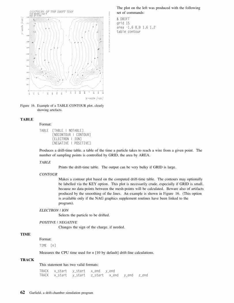
Figure 16. Example of a TABLE CONTOUR plot, clearlyshowing artefacts.

The plot on the left was produced with the followingset of commands:

& DRIFTgrid 15area -1.6 �.� 1.6 1.2table contour

TABLEFormat:

TABLE [TABLE | NOTABLE][NOCONTOUR | CONTOUR][ELECTRON | ION][NEGATIVE | POSITIVE]

Produces a drift-time table, a table of the time a particle takes to reach a wire from a given point. Thenumber of sampling points is controlled by GRID, the area by AREA.

TABLEPrints the drift-time table. The output can be very bulky if GRID is large.

CONTOURMakes a contour plot based on the computed drift-time table. The contours may optionallybe labelled via the KEY option. This plot is necessarily crude, especially if GRID is small,because no data-points between the mesh-points will be calculated. Beware also of artifactsproduced by the smoothing of the lines. An example is shown in Figure 16. (This optionis available only if the NAG graphics supplement routines have been linked to theprogram).

ELECTRON | IONSelects the particle to be drifted.

POSITIVE | NEGATIVEChanges the sign of the charge, if needed.

TIMEFormat:

TIME [n]

Measures the CPU time used for n [10 by default] drift-line calculations.

TRACKThis statement has two valid formats:

TRACK x_start y_start x_end y_endTRACK x_start y_start z_start x_end y_end z_end


Defines a track to be used by the DRIFT TRACK instruction. Defaults are the previous values, theyare not preset. The track is shared between the field, drift and signal sections. The track is alwaysstraight, even if the cell has been described in polar coordinates.

The second format is recognised only with future extensions in mind. All drift-lines start at z=0, nomatter the z at which the track is located. See the remarks under AREA.



z_start z-coordinate of begin point [cm].



z_end z-coordinate of end point [cm].

TRAPFormat:

TRAP n

Determining that a particle hits a perhaps very thin wire, is a remarkably difficult task. One of thecriteria used by Garfield is that every particle traveling by a wire at a distance smaller than n wire-radii,is considered to be caught, provided the wire can, given its charge, in principle attract the particle(unless the CHECK-ALL-WIRES option is in effect). Within this area, the alternate (dedicated) inte-gration algorithm takes over and it might therefore be a good idea to choose a large value for n. [Thedefault is 5.]

Figure 17. An example of an x(t)-correlation plot.

XT-PLOTFormat:

Program input 63

XT-PLOT [DATASET dataset [ member ]] [REMARK remark] [ANGLE φ]

[X-RANGE xmin xmax] [X-STEP x] [JUMP jump][ITERATIONS { iter_max | YES | NO or OFF } ]

[PRECISION e] [LEFT-ANGLE-RANGE Θminleft Θmaxleft] [RIGHT-ANGLE-RANGE Θminright Θmaxright]

[PRINT-XT-RELATION | NOPRINT-XT-RELATION][PLOT-XT-RELATION | NOPLOT-XT-RELATION]

(Only for Cartesian cells; see also the more refined ARRIVAL instruction.) Calculates an ordinaryx(t)-correlation for all sense wires located in the current area. XT-PLOT also calculates the integrateddiffusion coefficient, and plots this as a dashed line in the graph. A description of the algorithm can befound in Section 4.3.3 on page 112.

The proper functioning of this call depends on the settings of several global variables: LINES,EPSILON, AREA. Greater or lesser precision can be obtained by playing with the local variable PRE-CISION and the ITERATIONS switch. Iterations are expensive in terms of CPU time and their numbershould therefore be limited; they are however instrumental in finding a good approximation of the trueminimum. As a general rule, the number of iterations gets lower when the LINES parameter isincreased (LINES drift-lines are used for an initial search from the wire to the edges). This search canbe made more efficient by limiting the ANGLE-RANGE, even to the point that LINES can be madesmaller.

The graph made by the XT-PLOT instruction consists of two lines: the drift time (drawn asFUNCTION-1, see the graphics REPRESENTATION instruction, Section 3.12.10) and the diffusion(drawn as FUNCTION-2). Points for which the results of the computation are not considered fullyreliable, are not drawn. There may therefore be gaps in the curves. If a curve segment consists of onlyone point, then a marker is used to show the point.

An example of this kind of plot is shown in Figure 17 on page 63.

dataset The x(t)-relations will be written to the dataset if dataset is specified. The dataset mayexist before program execution, in which case the new relations will be appended. Amember name member may optionally be specified, but it is not used anywhere in theprogram. The dataset is written in the format '(L1,1X,4(E15.8,2X),A)', the logical indicateswhether the point is reliable or not. The reals are x, the minimum t, the value of y forwhich the minimum occurs and the integrated diffusion. The text provides additional infor-mation on the quality of a point. A program reading the file should be able to recognisethe phrase 'Not available' which is substituted for a number that has not been evaluated orthat is not considered to be sufficiently reliable. Refer to Section 2.3.2 on page 10 fordetails about the file format and naming conventions.

remark By default, the remark states the number of the wire the present x(t)-relation applies to andthe φ for which it has been calculated. This defaults is overriden if remark present.

φ The angle φ (defined in Section 4.3.3 on page 112) should be in the range −450 to +450.

x Sets the interval in x between 2 points for which the minimum t is calculated (thex-coordinate of the wire is one of the points, the range is taken from the AREA). Thedefault value of x is some reasonable number (1, 2 or 5 times some power of 10) such thatthe x(t) will contain about 20 data-points.

xmin-xmax The x(t) relation is by default sampled at regularly spaced points on the whole x-range ofthe drift-area. By setting xmin and xmax you may restrict this range. [Defaults: respec-tively the lower and upper x-bound of the area.]

jump The drift-time for one every jump points is minimised, this is accurate but time-consuming.If the drift-line which minimises t for one x, gives a minimum t for other x in the neigh-bourhood too, an interpolation is usually adequate (skipping the minimising procedure).Note that interpolations on drift-lines are usually accurate only up to the 3rd digit. Bydefault the parameter has a value of 1, i.e. all points are minimised.


iter_max The x(t) algorithm iterates at most iter_max [5, by default] times to find a minimum drift-time. Restricting the number of cycles should only be seen as a safeguard against loopingwithout actually getting nearer to a minimum. It is normally preferable to relax the conver-gence criteria (see ε) if CPU time consumption becomes unbearable.

ε The local precision, used to check whether convergence has been achieved, see Section4.3.3 on page 112. Values less than 10−4 are useless in single precision compilations.

θmin, θmax Limits the angles being explored in the initial search. The 0� line for θminright and θmax

right is thepositive x-axis, for θmin

left and θmaxleft the negative x-axis. The program will recover from an

ill-chosen angle-range, be it at the expense of many iteration cycles. In the presence of astrong magnetic field, the drift-line over which the first electrons reach the wire, can have asubstantial angle with respect to the x-axis. It is advisable under such circumstances tolimit the search to angles around this drift-line; the DRIFT WIRE instruction can be used tomake a good guess. [Defaults are -10� and +10�, both left and right, irrespective of themagnetic field, if any.]

PRINT-XT-RELATION Requests a printout of the x(t) relation [default].

PLOT-XT-RELATION Requests a graph of the x(t) relation [default].

WRITE-EQUAL-TIME-CONTOURSFormat:

WRITE-EQUAL-TIME-CONTOURSDATASET dataset [member] [REMARK remark]

A call that can be issued once a drift-line plot with contours has been made. The points that served todraw the equal drift-time contours are written to (member member of) the file dataset. For easierreference, you may add a remark. The DATASET and REMARK keywords may be omitted, providedthe order of the arguments is respected: e.g. member has to be specified if you wish to have a remark.Refer to Section 2.3.2 on page 10 for details about the file format and naming conventions.

WRITE-TRACKFormat:

WRITE-TRACKDATASET dataset [member] [REMARK remark]

Writes a 'prepared track' (see PREPARE-TRACK) to a dataset. The dataset is written when thecommand is issued, in contrast to most other WRITE statements which are delayed until the data to bewritten are available. This statement should therefore be preceded by PREPARE-TRACK. TheDATASET and REMARK keywords may be omitted, provided the order of the arguments is respected:e.g. member has to be specified if you wish to have a remark. Refer to Section 2.3.2 on page 10 fordetails about the file format and naming conventions.

Example of a valid drift section:

& DRIFT* Plot drift-lines starting from the surface of the D wires.SELECT DDRIFT WIRE* Plot 1�� drift-lines from a track, without equal time contours.TRACK -1 -1 -1 1LINES 1��DRIFT TRACK TIME-GRAPH, VELOCITY-GRAPH, NOCONTOUR* Calculate x(t)-relations for the C wires, output them to a dataset.SEL CXT DATA 'DISK$USER:[MYDIR.XT]XT_DC1.DAT' ...

REMARK "Override the default for fun."

Program input 65

3.10 The signal sectionThis section simulates the signal induced on the sense wires resulting from the passage of a charged particlethrough the chamber. It includes an option to write the signals to a file for analysis by Sceptre, Spice or an otherelectronic circuit analysis program. The header line to enter this section is & SIGNAL. The following instructionsare valid:

AREASee the drift-section, the drift and signal section have a common drift area.

AVALANCHEFormat:

AVALANCHE{EXPONENTIAL mean | FIXED factor | GAUSSIAN mean rel_dev | TOWNSEND}

This instruction sets the multiplication factor to be used in the signal simulation. The avalanche multi-plication factor is only used in the final stage as a global scaling factor for the signals. Multiplicationfactors smaller than 1 are always replaced by 1.

EXPONENTIALThe multiplication factors are drawn from an exponential distribution with fixed averagemean.

FIXEDAll multiplication factors are set equal to factor.

GAUSSIANThe multiplication factors are drawn from a Gaussian distribution with an average meanand a standard deviation relative to the average rel_dev.

TOWNSENDThe multiplication factors are drawn from an exponential distribution with an average equalto the exponential of the integrated Townsend coefficient over the electron drift-line. Thisoption can only be used if the Townsend coefficients were entered during the most recentgas section. Note that the measurement of Townsend coefficients is notoriously difficultand that an inaccuracy in the Townsend coefficient is amplified by the exponentiation in thecomputation of the multiplication factor. The calculated multiplication factor can thereforeeasily be off by an order of magnitude.

CHECKFormat:

CHECK {AVALANCHE | DIFFUSION | CLUSTER}[RANGE mult_min mult_max][FROM x y]

[N n] [BINS n_bins]

A debugging instruction that checks the proper functioning of the random number generators of thesignal section.

AVALANCHEPlots the avalanche multiplication factor distribution. If the avalanche type has been set toTOWNSEND, the starting point of the drift-line has to be specified via FROM x y.

CLUSTERPlots a histogram of the number of clusters generated on the current track, the track has tobe set and it may not be a point. In addition, a histogram of the cluster-size distributionwill be generated (overlaid with the appropriate functions if available).

DIFFUSIONPlots the arrival time distribution for a drift-line starting from (x,y).


nSets the number of entries in the histograms (default 10000).

n_binsSets the number of bins in the histogram to be generated.

RANGEIs only effective with AVALANCHE, sets the range of the histogram (default 1 to 1010).

x, yStarting point of the drift-line to be examined.

EPSILONSee the drift-section.

FOURIERFormat:

FOURIER n_Fourier

(Only relevant for periodic cells). Sets the number of Fourier terms in the ion-tail calculations ton_Fourier. The convolution equations for the ion-tails are (in case of periodic cells) solved via Fouriertransforms (each term in the series is a matrix similar to a capacitance matrix). Using a large numberof terms increases the accuracy but may also lead to an enormous amount of disk I/O (the matrices arestored on an external scratch file). A doubly periodic cell with 100 wires for instance, requires (in thestandard parameter setting) a frequent manipulation of 2.56 × 106 complex numbers, which makes itimpracticable on most computers. You may choose n_Fourier yourself, it should be an integral powerof 2 (in view of the FFT), 1 is allowed and is default.

GET-TRACKFormat:

GET-TRACK dataset [member]

Retrieves a 'prepared track' (see PREPARE-TRACK in the drift section) from a dataset written by a callto WRITE-TRACK. The track begin and end points are stored in such a dataset, hence there is no needto enter them again via TRACK. Be sure that you load the cell and gas data that were active when youcreated the dataset. The prepared track is not used in the signal calculations unless you specifyINTERPOLATE-TRACK on the SIGNAL statement.

dataset The name of the dataset in which the prepared track can be found. Refer to Section 2.3.2on page 10 for details about the file format and naming conventions.

member The member name of the prepared track, a string of up to 8 characters. You may use awildcard for this item: TR*1 will for instance match TRACK-1 or TR1 but notTRACK122. The default is an asterisk, matching every member name. The first memberin the dataset that is a prepared track and matches the member name you specify, will beread. The %INDEX command can be used to find out which members have been stored ina given dataset.

ION-LINESFormat:

ION-LINES n_ions

The calculation of the ion-tails involves the drifting towards the anode of n_ions ions from equallyspaced points around all sense wires (if CROSS-INDUCED has been inhibited) or from all wires (ifCROSS-INDUCED has been enabled) hit by at least one cluster. One can sometimes save a lot ofCPU time by reducing n_ions without loosing too much accuracy. [The default is 10.]

OPTIONSFormat:

OPTIONS [CLUSTER-PRINT | NOCLUSTER-PRINT][CLUSTER-PLOT | NOCLUSTER-PLOT][ION-PLOT | NOION-PLOT][SIGNAL-PLOT | NOSIGNAL-PLOT]

Program input 67

In addition to the general options and the options of the drift section, a few local options are availableto control the amount of output:

CLUSTER-PLOTPlots the track of the charged particle, the positions of the clusters and drift-lines of theclusters.

CLUSTER-PRINTPrints the same data CLUSTER-PLOT plots.

ION-PLOTControls the plotting of the ion-drift-lines used for the calculation of the ion-tail, if this partof the calculation has been requested. The ion-tail is calculated (and therefore plotted) onlyonce per signal section unless a parameter affecting it is changed.

SIGNAL-PLOTPlots the signals on the sense wire; the signal is not plotted if it is identically zero, forinstance due to a poor choice for RESOLUTION.

REPEATFormat:

REPEAT times

The next simulation instruction will be carried out times times [default is 1]. Note that the setting ofthis parameter has some bearing on the interpretation of the OLD and NEW keywords on SIGNAL.

Please consider using a DO-loop instead, REPEAT is scheduled to disappear in some future release.

RESOLUTIONFormat:

RESOLUTION t_start t_step

This statement changes the time-window of the signals, both in the dataset and in the plots.

t_start The first point in time at which the signal is to be sampled relative to the time the particletraversed the cell [in μsec, default is 0 sec].

t_step The signal is output at MXLIST (usually 200) points spaced by t_step [in μseconds, defaultis 0.01 μsec].

SELECTFormat:

SELECT wire-codes

SELECT will mark the wires with a code appearing in the argument so that the signal calculationhandles them as the sense wires. The signals on wires with codes between brackets will be summed.For example: S(PT)R will give as output signals (i) separate signals for all 'S' wires, (ii) the signals onall 'P' and 'T' wires added together to give only one signal and (iii) a separate signal for each of the 'R'wires. Wires can also be selected using their number (consult the table obtained with the optionCELL-PRINT). [By default all wires with code 'S' are used as sense wires.]

SIGNALFormat:

SIGNAL [AVALANCHE | NOAVALANCHE][DIFFUSION | NODIFFUSION][ION-TAIL | NOION-TAIL][NEW | ADD][NOCROSS-INDUCED-SIGNAL | CROSS-INDUCED-SIGNAL][NOELECTRON-PULSE | ELECTRON-PULSE][NOINTERPOLATE-TRACK | INTERPOLATE-TRACK]

Marks the beginning of a simulation which will be repeated REPEAT times. It assumes that you havedefined a track on beforehand (TRACK statement). You may also wish to select an avalanche type, anumber of Fourier terms and a number of ion drift-lines before carrying out the simulation. Further, a


WRITE statement before this instruction is needed if you would like the signals to be written to adataset. Note that at least some output has to be requested (via OPTIONS or WRITE), otherwise thesimulation will not be performed. Signal simulations are potentially highly CPU time consuming oper-ations.

AVALANCHETakes the avalanche near the wire-surface into account, the type of avalanche can beselected by the user, see AVALANCHE.

CROSS-INDUCEDCalculation/no calculation of the cross-induced signals i.e. the signal induced on wire i byions drifting away from wire j (i ≠ j). Be careful when using it: an external scratch file isused to store the intermediate results, considerable amounts of disk I/O may therefore resultin particular if there are many (sense)wires.

DIFFUSIONTakes longitudinal diffusion of the electrons along the drift-lines into account. There is noway in this program to allow lateral diffusion.

E-PULSEAdds spikes to the signal, indicating the time the electrons hit the wire. No detailedinduced current calculation is performed, rendering this option rather useless.

INTERPOLATE-TRACKRequests the prepared track (see PREPARE-TRACK) be interpolated during the signal sim-ulations. By default all drift-lines are calculated when they are needed - this tends to berather CPU-time consuming for large numbers of signals.

ION-TAILAdds ion-tails to the signal, the way the ion-tails are calculated is to some extent under usercontrol (see FOURIER and ION-LINE). The program attempts to calculate the ion-tailsfairly precisely.

NEW/ADDCreate a new signal or add the results to the previous signals. NEW is default for the firstcall in the section ADD for all following calls. The signals are cleared each time if NEWhas been specified and REPEAT has been set to a value different from 1. ADD can forinstance be used to study two-track separation.

Program input 69

Figure 18. Clusters and electron drift-lines. The dashed linerepresents a track segment. At intervals gener-ated according to an exponential distribution,clusters have been put. An electron drift-line hasbeen calculated from each cluster and the inte-grated diffusion and integrated Townsend coeffi-cient have been evaluated.

Figure 19. Ion drift lines. When the clusters shown inFigure 18 on page 70 reach a wire, they gen-erate an avalanche. The ions that are producedin the avalanche drift (slowly) away from thewire as shown in this Figure.

Figure 20. Example of a signal. This graph shows thesignal induced by the ions moving away from thecentral wire of Figure 18. The small spikes arethe result of diffusion, the broader structuresreflect the various (groups of) clusters.

The plots shown on this page have been produced withthe following set of commands:

& SIGNALopt cl-pl ion-pl debug drift-plarea -1.5 1.5 +1.5 3.5track 1.� 2.1 1.2 2.7resolution 1 �.��5signal

TRACKFormat:


TRACK x_start y_start x_end y_end

Defines the track of a charged particle through the cell. The clusters will be generated at randomlydistributed points on this track. The track will be clipped, if necessary, to ensure that it lies entirely inthe drift-area. Defaults are the previous values, they are not preset. The tracks is shared between thefield, optimise, drift and signal sections. The track is always straight, even if the cell has beendescribed in polar coordinates.





TRAPSee the drift-section.

WRITE-SIGNALFormat:

WRITE-SIGNAL[DATASET dataset [member] ]

[REMARK remark][FORMAT {SPICE | SCEPTRE} ][STATE {OPEN | CLOSE | RESUME | SUSPEND} ]

Controls the output to dataset of the signals produced by subsequent SIGNAL instructions, no signal iswritten immediately. The STATE keyword would not normally be used together with DATASET; sucha usage is permitted however.

datasetA dataset name like 'SIGNALS SCEPTRE A' (CMS, mind the quotes !) or[VEENHOF]SIGNAL.DAT (Vax). The new signals will be appended as a new member ifthe dataset exists at the time the signals are being written. In contrast to most otherWRITE instructions, all keywords such as DATASET and REMARK are compulsory.Refer to Section 2.3.2 on page 10 for details about the file format and naming conventions.

remarkThis string will override the default comment stating the wire-number and the angle. Aremark may be specified by itself, i.e. without dataset, in which case only the previousremark (or the default) is replaced.

OPENOpens a dataset for writing signals, this is default when a dataset is specified explicitly.

CLOSECloses the dataset, forgetting its name.

RESUMEResumes writing to the dataset previously opened, the dataset name need not be specifiedagain.

SUSPENDTemporarily suspends writing of signals to the dataset, writing may be resumed later on.

SPICEThe dataset will be written in a Spice readable format.

SCEPTREThe dataset will be written in a Sceptre readable format.

Example 1: double track resolution (CMS file naming conventions)

Program input 71

& SIGNAL* First define a track, then set starting time and time intervalTRACK -�.5 -�.5 �.5 -�.5RESOLUTION 1.� �.�5* Open a file for the Spice output and select the sense wiresWR-SIG DATASET: 'SIGNALS SPICE B', FORMAT=SPICE* The signals on all 'S' type wires are to be summed. All other* wires are ignored. The simulation will therefore produce just* one output signal.SELECT (S)* Perform the simulationSIGNAL DIFFUSION NOAVALANCHE, NOE-PULSE ION-TAIL* Open a new file, for Sceptre output this time:WRITE-SIGNAL DATASET SIGNALS.SCEPTRE.B FORM SCEPTRE* redefine the track,TRACK -�.5 -�.6 �.5 -�.6* and add the new signals to the old ones, writing them to the* dataset. The selection of the sense wires remains unchanged.SIGNAL ADD

Example 2: using a prepared track (Vax file naming conventions)

& DRIFTtrack �.1 -�.9 �.1 �.9prepare-trackwrite-track 'disk$v8:[veenhof.signal]test.dat'

& SIGNALwrite-signal [-]test.datsignal interpolate-track diffusion noavalanche

A track is prepared and the result is written to a file which can be used for subsequent runs as shown below. Notethat the command to save the track is issued after the track has been prepared whereas the instruction to write thesignals to a dataset is issued before the signals are calculated. The INTERPOLATE-TRACK argument must bespecified for the prepared track to be actually used.

& SIGNALget-track 'disk$v8:[veenhof.signal]test.dat'write-signal [-]test.datsignal interpolate-track diffusion noavalanche

It is good practice to store cell, gas, track and other data related to one chamber in the same dataset. No confusioncan arise if there is only one member of each type because the GET instructions look only at members of theproper type. Use member-names to distinguish members of the same type.


3.11 The stop commandThe & STOP command allows decent program termination. & STOP will close all input and output files, close thegraphics system and then print a log of CPU time consumption, of plots produced during the run and a list ofdataset accesses. An EOF (end of file, usually control-Z) has roughly the same effect. The null input line, the EOFmark in interactive VM/CMS, is intercepted and subsequently ignored. Rather use & STOP or an EOF than aninterrupt, control-Y on Vax or control-Q on Apollo, if the program has been generating a metafile.

& STOP does not work from inside the various sub-sections: algebra, dataset, help, graphics etc.; control-Z doeswork. If you get stuck in one of those, try EXIT and then & STOP.

& EXIT and & QUIT are synonyms of & STOP.

Program input 73

3.12 Instructions valid in all sectionsThe instructions listed below are section independent. They may appear anywhere in the input (with the exceptionof the dataset, graphics and help sub-sections).

3.12.1 Global optionsOptions are switches that influence the behaviour of the instructions that follow. All sections have an instructionthat allows changing and displaying the settings of the options. The options mentioned here are global in that theyhave a meaning in every section. The options mentioned in the beginning of this chapter have a bearing on onlyone or perhaps a couple of sections and should therefore only be specified in an OPTIONS command in the appro-priate sections. You may freely mix global and local options in a single OPTIONS line.

OPTIONS Format:

OPTIONS [NODEBUG | DEBUG][INPUT-LISTING | NOINPUT-LISTING][NOIDENTIFICATION | IDENTIFICATION]

DEBUGPrints some critical intermediate results, useful only if you have a program listing. DEBUGdoes not require much CPU time but it tends to produce a lot of output.

Debugging is initially off by default but this can be overruled by the /DEBUG commandqualifier (on Vax), the DEBUG command line option (VM/CMS) and the -debug commandline option (Unix).

IDENTIFICATIONPrints the name of a few selected routines when they are called. Useful for tracing theprogram.

Tracing is initially off by default but this can be overruled by the /IDENTIFICATIONcommand qualifier (on Vax), the IDENTIFICATION command line option (VM/CMS) andthe -identification command line option (Unix).

INPUTEchoes the input instructions. This option is off by default when running interactively buton in batch.

3.12.2 Kernlib error messagesMainly for debugging purposes, you can control handling of error messages generated by the KERNLIB routines.

ERROR-HANDLING Format:

ERROR-HANDLING MESSAGE mess_id[PRINT {ALWAYS | NEVER | nprint} ][ABEND {NEVER | nabend} ]

Requests that the messages identified by mess_id, see the N001 writeup for details, are printed respec-tively always or never or nprint times. Program execution is respectively never terminated or atnabend+1'th occurence of the error. Both nprint and nabend are meaningful only in the range 0 to 100.

3.12.3 Printing a commentSAY Format:

SAY string

Will simply copy the string to the current output stream. Like in all other instructions, expressionsinside curly brackets are evaluated before the instruction is processed, that is, in this case, before thestring is printed. Thus, SAY can be used to do simple arithmetic. This instruction is frequently usedinside loops to print out the value of some global variable (see Section 3.2.1 on page 17).

Examples:


Say "Time left: {entier(time_left/36��)} hours, ...{entier((time_left-36��*entier(time_left/36��))/6�)} ...minutes, {time_left-6�*entier(time_left/6�)} seconds."

Say {arctanh(�.3)}

3.12.4 Comment linesComment Format:

* anything

The contents of the line is ignored. Mainly useful in input files and in batch.

3.12.5 Input translation tablesYou may wish to have a character you type translated into another, for instance a character not found on yourkeyboard. The TRANSLATE command helps you to achieve this. The translation table can be updated anynumber of times; each modification is valid from the point it was entered onwards. The translation table can bewritten to a Garfield library and be retrieved from the library later on.

Reading of the translation commands is subject to the translation tables in effect at the moment the command isissued.

TRANSLATE Format:

TRANSLATE [CYCLES ncycle][INTEGER | HEXADECIMAL] char_in[INTEGER | HEXADECIMAL] char_out ...

Specifies which characters are to be translated; you may list several translations on one line. Previouslyspecified translations remain in effect. Translations are cancelled by requesting a character is translatedinto itself; you may have to identify the character via its translation or its integer or hexadecimal code.

Translation of the input string is performed before the conversion to upper case, before the string issplit into words and before special characters are acted on.

The current translation table is displayed if the TRANSLATE instruction is entered without arguments.

By default no translation is performed, except on Vax where the tab character (hex 9) is translated intoa blank.

INTEGERMeans that char_in or char_out is the integer code, ASCII or EBCDIC as appropriate, ofthe character you wish to reference. The integer code must be in the range 0 to 255.

HEXADECIMALMeans that char_in or char_out is the hexadecimal code, ASCII or EBCDIC as appropriate,of the character you wish to reference. The hexadecimal code must be in the range 00 toFF and should be entered pure, i.e. without leading X' etc.

char_inThe character to be translated: either the character itself or its integer code or itshexadecimal code.

char_outThe character char_in is to be translated into, either the character entered as-is or its integercode or its hexadecimal code.

ncycleNumber of times the translation table should be applied to each input string. By defaulteach character is translated only once but you may request up to 256 translations. Toswitch translation temporarily off, specify 0.

GET-TRANSLATION-TABLE Format:

Program input 75

GET-TRANSLATION-TABLE dsname [member]

Retrieves the translation table member stored in the dataset dsname.

WRITE-TRANSLATION-TABLE Format:

WRITE-TRANSLATION-TABLEDATASET dsname [member]

lsqb;REMARK remark]

Writes the current translation table to member member of dataset dsname. You may add a remark foreasier identification later on.

3.12.6 Obtaining helpHELP Format:

? [search_string]

Provides on-line help, provided the additional files have been put in place. The help facility looks verysimilar to that on a Vax (where it really is the standard help utility). The information is organised inthe form of a tree. The major branches are the sections and sub-sections. Some more general informa-tion is also available near the root. At each level you are presented with a list of sub-topics. Choosingone of them, you may use wildcards for this, will take you one level higher in the tree. In wildcards,the asterisk (*) can represent any number of arbitrary characters, *IX matches both ASTERIX andIDEFIX. An asterisk at the end is always assumed in the help facility, hence A*R matches bothABRARACOURCIX and ASTERIX. A blank return brings you down by one level. You may at anytime type a question mark (?) instead of a sub-topic. The current item and the list of sub-topics arethen displayed again.

HELP or INFORMATION may be typed instead of the question mark.

3.12.7 Input from and output to datasetsInput Format:

< file_name [<< label]

The file is opened and its contents is read as input until the end of the file or the label, if specified, isreached. Within the alternate input file, input may be taken from another file and so forth (up to 10times). The label should be a string of up to 80 characters; the file will be read up to the end of thefile if specified as EOF, this is also the default action. Each file has its own label.

The input taken from a file is handled in exactly the same way as input from the terminal, hence thelines will be echoed if the INPUT option is on. Refer to Section 2.3.2 on page 10 for details about thefile naming conventions and the file format.

Input recording Format:

>> [file_name]

Input typed to the terminal will be recorded in the specified file. Type >> without argument to stoprecording input statements. Input recording is on by default in interactive runs and off in batch.

Output Format:

> [file_name]

Routes some of the output to the specified file. Type a > without argument to stop sending the outputto a file. This instruction applies mainly to output which might otherwise interfere with plots. Errormessages and warnings are always written to standard output. Refer to Section 2.3.2 on page 10 fordetails about the file naming conventions and the file format.

3.12.8 Shell commandsShell Format:

$ command


The command after the $ sign is not interpreted by Garfield but passed on to the program environment(CMS, DCL, Aegis, Unix). The command is passed on as is, without case conversion. This featurecan for instance be used to obtain a directory listing, to edit files, to send messages, to ask for the timeetc.

Running another program from inside Garfield should be avoided under VM/CMS. Also, executingexec files will sometimes cause the program to abend. In addition some common VM/CMS commandscannot be executed, see the writeup for VMPACK (Z305), routine VMCMS. Finally, take care to enterCMS commands in upper case.

Such restrictions do not seem to be present on Apollo and Vax. Don't try to run Garfield inside itself:the program write locks some of its log and working files. Some Vaxes have a very low sub-processquota; ask your system manager for more if needed.

To make a longer excursions into CMS, type:

$(CMS commands)RETURN

The 'excursion' method uses the CMS SUBSET mode, which offers some protection against typing commandswhich are illegal in this context.

To make a longer excursions to DCL (on a Vax), type:

$(DCL commands)LO

The DCL commands are executed in a sub-process that is essentially independent from the main process.

To make a longer excursions to Aegis (on Unix) type:

$(Aegis commands)return

The Aegis commands are executed in a sub-shell and are independent from the shell in which the program runs butshell and sub-shell share the same I/O streams. The choice for Aegis as shell is arbitrary and could easily bechanged to the C shell. Your environment on Unix systems (Cray, Sun) is a C shell:

$(Unix commands)exit

3.12.9 Garfield library manipulation commandsThese commands allow obtaining information about a Garfield library, marking some of its members for deletion,purging the library, listing some members etc.

An editor can be used to modify the files, but this is not recommended since retrieval of some types of members(cell, gas, track ...) relies without checking on the integrity of the data. It is safe to remove complete membersmanually.

If the % is the only character on the line, further dataset commands can be entered without the % sign, until youtype EXIT, which will return you to where you came from. There are a few commands that can not be executed inthis fashion.

Both the member and the type may be of the wildcard type, the match-all character being the asterisk '*'. Noasterisk at the end of the strings is assumed.

% DEFAULTFormat:

% DEFAULT [default_dataset_name]

Program input 77

(VM/CMS and Vax only) This command allows you to establish defaults for the various components ofa dataset name on Vax/VMS: node, disk, directory, file name, file type, version number and onVM/CMS: file-name, file-type and file-mode. All components can be overruled in the actual datasetspecification. The initial value is .DAT without wildcard for Vax and file-type INPUT, file-mode *(any) for VM/CMS.

Under VM/CMS, an equal sign (=) should be substituted for a component of the dataset name forwhich you do not wish to establish a default. You do not have to enclose the dataset name by quoteshere, except if you have used equal signs, since these are normally separators. Dots may be usedinstead of blanks to separate the fields. When a dataset is referenced, fields specified as = are replacedby the corresponding default. If the file-name or file-type is still an equal sign after this substitution, itis set to * (match anything). The file-mode is set to the letter of the first RW disk for write andread-write access and to * for read access, if both the default and the specified file have an equal signas mode.

Examples: (VM/CMS)

%default '* input ='% def GARFIELD.*.A

In the first example, the mode has to be entered explicitly, the type defaults to INPUT and the namecan be anything.

This command can not be issued from within a dataset subsection.

% DELETEFormat:

% DELETE dataset member [type]

Marks member in dataset for deletion. The member is not actually removed, that is done by thePURGE command. SCRATCH is a synonym for DELETE.

% DUMP-HELP-FILEThis debugging command dumps the entire contents of the help file, thus allowing to check the integ-rity of the tree structure.


% INDEXFormat:

% INDEX dataset [member [type] ]

Prints a listing of the members contained in dataset. DIRECTORY is synonymous to INDEX.

% LISTFormat:

% LIST dataset [member [type] ]

Prints the contents of member of type type in dataset. If the member is omitted, all members will belisted. PRINT is synonymous to LIST.

% RECOVERFormat:

% RECOVER dataset member [type]

Is the converse of DELETE: unmarks member in dataset, thus making it readable again. RESCUE issynonymous to RECOVER.

% PACK-HELP-FILEFormat:

% PACK-HELP-FILE [TRANSLATE | NOTRANSLATE]

This command will translate the normally legible help file into a direct access file which can be read bythe help routines. You should not have to do this yourself, unless you're responsible for file updating.Make sure that no version of the packed help file is available before you issue this instruction.


The legible help file should be called GARFIELD RAWHELP on VM/CMS, HELP_RAW$GARFIELDon Vax/VMS and garfield.rawhelp on Unix systems. The packed help file is calledGARFIELD PACKHELP on VM/CMS, HELP$GARFIELD on Vax/VMS and garfield.packhelp onUnix systems.


The TRANSLATE options exists only on IBM interactive systems, where it helps to correct an error insome old ASCII to EBCDIC conversion tables. Curly brackets (8B and 9B) are sometimes improperlytranslated (C0 and D0).

% PURGE datasetFormat:

% PURGE dataset

Removes deleted members from dataset. This instruction may hurt ! Once purged, no recovery ispossible (unless you made a backup of course).

3.12.10 Graphics instructionsModifies or displays the GKS graphics settings. The settings can be changed at all times and any number of times.They take effect immediately and do not affect plots that may already be on a metafile. If the exclamation mark isthe only character on the line, further graphics commands can be entered without the ! sign, until you type EXIT,which will return you to where you came from.

For information about GKS, see for instance the excellent but slightly outdated book by Hopgood et al. [5]. Detailsabout the most commonly used GKS at CERN and associated institutes, GTS-GRAL/GKS, are to be found in [6].This facility was only tested with GTS-GRAL/GKS.

! ACTIVATE-WORKSTATIONFormat:

! ACTIVATE-WORKSTATION wsname

Activates the workstation named wsname. The workstation should already be defined and open.

! ADD-WORKSTATIONFormat:

! ADD-WORKSTATION wsname[TYPE type | GKS-IDENTIFIER gksid][CONNECTION-IDENTIFIER conid | OFFSET offset]

[FILE-NAME file]

Adds a workstation to the workstation table. Depending on the system, a workstation named TER-MINAL or one named METAFILE, or both, can be predefined. The attributes of these two work-stations are set with the command line qualifiers.

A workstation, once added, can be opened and then activated after which it will receive graphicsoutput.

! CLOSE-WORKSTATIONFormat:

! CLOSE-WORKSTATION wsname

Closes the workstation named wsname. The workstation should be defined and open but not active.

! COLOURFormat:

! COLOUR colour_name [RED red] [GREEN green] [BLUE blue] [WORKSTATION wkid]

Defines a new colour to be added to the workstation tables, provided it has colour facilities. If yourterminal has them, take care to transmit the right workstation identifier to the program during start-up inorder to use them. On Vax and CMS you can do so via command line parameters, on other machines

Program input 79

you may have to recompile. The program can not determine which device is going to be used to lookat WISS and metafile output and allows all colours for these. You may redefine a colour any numberof times; the total number of colours you may define depends on the GKS you're using but rarely morethan 20 colours are allowed.

If you omit the colour_name, all known colour representations are listed. If you specify it but omit thecolour intensities, only the representation of the chosen colour is displayed.

colour_nameThe name of the colour you wish to (re)define or to inquire about. This should be a stringof at most 20 characters. The recommended format is that of the type used internally forinput string matching: segment1-segment2-segment3... where each of the segments can haveone hash (#) indicating the point of minimal abbreviation. For instance, 'BL' matches thecolour names 'BL#UE' and 'BL#ACK', 'D-GR' matches 'D#ARK-GR#EEN' but not'DARK-GR'.

All workstations have 2 predefined colours: BACKGROUND, with zero intensity for eachof the colours, and FOREGROUND, full intensity for each.

redThe intensity of red on a scale of 0 to 1.

blueThe intensity of blue on a scale of 0 to 1.

greenThe intensity of green on a scale of 0 to 1.

wkidThe workstation identifier on whose state list the colour is defined or is to be defined. Thisparameter should be left for the time being at its default [1].

! DEACTIVATE-WORKSTATIONFormat:

! DEACTIVATE-WORKSTATION wsname

Deactivates the workstation named wsname. The workstation should already be defined, open andactive.

! DELETE-WORKSTATIONFormat:

! DELETE-WORKSTATION wsname

Deletes the workstation named wsname. The workstation should be defined. All information about aworkstation is lost once it has been deleted.

EXITLeaves a graphics sub-section.

! GET-COLOURSFormat:

! GET-COLOURS dsname [member]

Reads a list of colours from a dataset, overwriting any colours you may have defined previously.

dsnameThe name of the Garfield library that contains the member you wish to load.

memberThe name to be member to be read.

! GET-REPRESENTATIONFormat:

! GET-REPRESENTATION dsname [member]


This instruction retrieves a representation table written by ! WRITE-REPRESENTATION. Colourtables should be loaded before the representation tables since the representation colour references areresolved while reading. The colours may be redefined afterwards if needed; unresolved colours are setto FOREGROUND.

dsnameThe name of the dataset from which the representation table should be read.

memberThe name of the member you wish to read.

! INQUIRE-DEFERRAL-UPDATE-STATE

! INQUIRE-DEFERRAL-UPDATE-STATE [wsname]

Reports the deferral, update and regeneration mode and also the screen state for workstation wsname.If the workstation name is omitted or is set to a *, then the information is shown for all known work-stations.

! INQUIRE-LEVEL-GKSReturns the GKS level of the GKS with which you are running.

! INQUIRE-OPERATION-STATEReturns the operation state, in order of increasing GKS activity: GKS closed, GKS open, workstationopen, workstation active and segment active. Segment active should in principle not occur. Work-station active is the minimum required to produce output and this should be the normal state in whichyou find GKS.

! INQUIRE-WORKSTATIONSLists all workstations which have been defined, the state in which they are and the files associated withthem, if any.

! OPEN-WORKSTATIONFormat:

! OPEN-WORKSTATION wsname

Opens the workstation named wsname. The workstation should already be defined.

! OPTIONFormat:

! OPTION [NOCLEAR-AFTER-PLOT | CLEAR-AFTER-PLOT][CLEAR-BEFORE-PLOT | NOCLEAR-BEFORE-PLOT][NOGRID-PLOT | GRID-PLOT][LINEAR-X | LOGARITHMIC-X][LINEAR-Y | LOGARITHMIC-Y][TIME-STAMP | NOTIME-STAMP]

A few aspects of plotting that do not fit in the REPRESENT command and are not workstation relatedeither, have been grouped in the graphics OPTION command. Global options can not be mixed withgraphics options.

CLEAR-AFTER-PLOTWhen a plot is complete, the program waits until you hit the return key before it proceeds.With this option on, which is not the case by default, the screen is cleared after you hitreturn. This is useful on Tektronix-4014 and similar terminals.

CLEAR-BEFORE-PLOTClears the screen before a plot is made. This is default for all devices; you will want toswitch this option off when overlaying 2 consecutive plots. The graphics REPRESENTcommand allows you to change for instance the colours in between the plots.

GRIDSwitching on GRID-PLOT, will cause a coordinate grid to be overlaid on the plot. Thecoordinate grid lines simplify reading values from the graphs.

Program input 81

The appearance of the coordinate grid can be modified to some extent by the !REPRESEN-TATION statement; by default dotted lines are used. The number of grid lines is deter-mined by the program from the range of values the axis covers; an attempt is made to drawthe grid lines at reasonable numerical values. The GRID parameter has no relation whatso-ever with the coordinate grid.

Grids are drawn on all plots, until the option is switched off again.

log/linearAllows to see certain plots on a log scale. Garfield feels free to change the value of theseparameters, for instance for the gas plots.

TIME-STAMPWill plot a line indicating date and time in the upper right hand corner of each graph that issent to a metafile.

! REPRESENTATIONFormat:

! REPRESENT item [attribute_1 value_1] [attribute_2 value_2] ...

This instruction allows you to change the appearance of the plots. The term item is used here to desig-nate a basic component of a plot, such as the axes, the title, a drift-line, a set of contours etc. Theitem's come in 4 types, called primitives in GKS terminology: polyline, polymarker, text and fill area.Some items, such as equal time contours, are plotted using more than one primitive, in this casepolyline and polymarker. The way a primitive is rendered on the output device is controlled by a seriesof attributes, for instance the colour of a line, the font of a piece of text etc. It are the attributes thatyou can change using the REPRESENT graphics instruction.

item Per REPRESENT instruction, you may change the attributes of only one primitive associ-ated with only one item. For instance, you are not allowed to request in a single REPRE-SENT statement that COMMENT must have line type DOTTED and text font -7(COMMENT exists as a text and as a polyline item). The primitive is determined from theattributes you list.

If you omit item, the representation of all items will be displayed. If you specify item butomit the attributes, the representation of item will be displayed, once for each of the primi-tives it uses.

BOX-TICKMARKS(Polyline) The lines used to draw the coordinate system.

COMMENT(Polyline) Additional lines sometimes help to clarify the plot, such lines forinstance separate in the drift-time graph the curves for different places wherethe particles end up.

COMMENT(Text) The pieces of information about the cell, the gas etc plotted underneaththe title.

CONTOUR-HIGHLIGHTED(Polyline) Some contours, usually every 5th, are highlighted.

CONTOUR-NORMAL(Polyline) The contours of the field but also of the drift-time when plotted viaTABLE - for highlighted contours see above.

C-WIRE(Polymarker) The marker to be used for C type wires when theWIRE-MARKERS option of the cell section is active.


DIELECTRICA(Fill Area) The dielectrica in the cell.

DRIFT-CONTOUR(Polyline) Contours of equal arrival time interpolated on drift-lines.

DRIFT-CONTOUR(Polymarker) When the distance between interpolated points on the drift-lines islarger than a certain threshold value, a marker is put on the drift-line instead.

DRIFT-LINE(Polyline) Drift-lines of electrons and ions.

FUNCTION-1(Polyline) The main function in a plot, usually this is the only curve beingdrawn. This type of line is also used for the vector plot in the field section.

FUNCTION-1(Polymarker) When a portion of the curve of the primary function consists ofonly one point, a marker is used rather than a line.

FUNCTION-2(Polyline) The second function drawn in a plot, used for instance for the inte-grated diffusion in the x(t) plot.

FUNCTION-2(Polymarker) When a portion of the second function consists of only one point,a marker is used rather than a line.

FUNCTION-3(Polyline) The third function drawn in a plot. Not yet used.

FUNCTION-3(Polymarker) When a portion of the third function consists of only one point, amarker is used rather than a line. Not yet used.

GRID(Polyline) The grid indicating the coordinates in a plot.

LABELS(Text) The labels are the annotations along the axes.

MESSAGE(Text) The line asking you to hit return when you have seen enough of a plot.

NUMBERS(Text) The numbers indicate the coordinate values along the axes.

OTHER-WIRE(Polymarker) The marker to be used for wires with a code letter other than C,P or S when the WIRE-MARKERS option of the cell section is active.

PLANES(Polyline) The equipotential planes in the cell.

P-WIRE(Polymarker) The marker to be used for P type wires when theWIRE-MARKERS option of the cell section is active.

S-WIRE(Polymarker) The marker to be used for S type wires when theWIRE-MARKERS option of the cell section is active.

TITLE(Text) The global title of the plot.

Program input 83

TRACK(Polyline) The track of a particle traversing the chamber as defined by theTRACK statement. Such tracks are not the drift-lines of electrons or ions.

TRACK(Polymarker) If the track consists of a single point, a marker is plotted.

TUBE(Polyline) The tube surrounding the wires as defined by the TUBE statement inthe cell section.

WIRES(Fill Area) Wires are plotted with fill area rather than polyline ! This is doneto allow them to be picked in GRAPHICS-INPUT.

attribute The attributes you specify must be all of the same type and consistent with the item ofwhich you wish to change the appearance. The labeling of the various attributes followsclosely the GKS terminology (see [5]) with the exception of the colours. Colours are speci-fied by a name previously defined using !COLOUR. Usually, drastic abbreviations aretolerated provided no confusion can arise.

CHARACTER-EXPANSION-FACTOR(Text) The deviation from the designer specified ratio height/width of a char-acter. [Default is 1.]

CHARACTER-SPACING(Text) Adds more space between characters. [Default is 0.]

CHARACTER-HEIGHT(Text) Height of the characters in world coordinates. Characters are plotted byGarfield using normalisation transformation 0, for which the scale of the wholeplot, including the blank area surrounding the coordinate box, ranges from 0 to1 both in x and in y. [Defaults: 0.01 for annotations and comments, 0.02 forthe title.]

FILL-AREA-INTERIOR-STYLE(Fill area) The way the areas are filled, you have the choice between 3 values:

HATCHEDThe area will be filled by a series of parallel lines, the type ofwhich can be chosen by the FILL-AREA-STYLE-INDEX.[Default for dielectrica.]

HOLLOWThis looks like a line: the border is drawn but the interior is leftempty. [Default for wires.]

PATTERNThe area will be filled by the pattern selected byFILL-AREA-STYLE-INDEX.

SOLIDThe area will be filled entirely in the colour you choose.

FILL-AREA-STYLE-INDEX(Fill area) The hatch or pattern type you wish to use. [Default: -111 fordielectrica when using GTS-GRAL.]

FILL-AREA-COLOUR(Fill area) The colour used to fill the area. This can be either BACKGROUND(in which case the corresponding item will not be visible), FOREGROUND orone of the colours you defined yourself via the !COLOUR command. [Default:foreground colour.]


FILL-AREA-PATTERN-SIZE(Fill area) When you choose pattern as fill area style, you may change the sizeof the pattern box using this attribute. [Not used by default]

FILL-AREA-REFERENCE-POINT(Fill area) When you choose pattern as fill area style, you may choose a refer-ence point of the pattern box using this attribute. [Not used by default]

LINETYPE(Polyline) The sort of line: you may either choose an implementation dependent(negative) number or one of the following values:

DASHEDThe line will consist of a series of dashes: - - - - - . [Default forcomment lines and equal time contours.]

DASH-DOTTEDThe line will be an alternating series of dashes and dots: .-.-.-.-.

DOTTEDThe line will consist of a series of dots: .........

SOLIDThe good old solid line. [Default for most lines.]

LINEWIDTH-SCALE-FACTOR(Polyline) The width of the line compared to default. This attribute is fre-quently ignored. [Default: 1.]

MARKER-TYPE(Polymarker) The sort of marker: you may either choose an implementationdependent (negative) number or one of the following values:

ASTERISKThe markers are small stars: '*'. [Default.]

CIRCLEThe markers are circles: '&cdot.',

CROSSThe markers are crosses: ×.

DOTThe markers are dots: '.'.

PLUSThe markers are plus signs: '+'.

MARKER-SIZE-SCALE-FACTOR(Polymarker) The size of the markers compared to their default size. The sizeof a marker compared to the overall scale of the plot may vary from one outputdevice to another. The plots in this manual have been made with a size of 0.5.[Default: 1, except for equal time contours where 0.25 is used.]

POLYLINE-COLOUR(Polyline) The colour used for the lines. This can be either BACKGROUND(in which case the corresponding item will not be visible), FOREGROUND orone of the colours you defined yourself via the !COLOUR command. [Default:foreground colour.]

POLYMARKER-COLOUR(Polymarker) The colour used for the marker. This can be either BACK-GROUND (in which case the corresponding item will not be visible), FORE-GROUND or one of the colours you defined yourself via the !COLOURcommand. [Default: foreground colour.]

Program input 85

TEXT-COLOUR(Text) The colour used for the text. This can be either BACKGROUND (inwhich case the corresponding item will not be visible), FOREGROUND or oneof the colours you defined yourself via the !COLOUR command. [Default:foreground colour.]

TEXT-FONT(Text) The font used to plot the text. Most of the 'special' fonts (greek, gothic,italics) are only available in STROKE quality, see TEXT-PRECISION below.Text fonts are largely implementation dependent; the GKS manual for yourinstallation should contain a list of fonts. The plots in this manual have beenmade with GTS-GRAL font -104. [Default: 1.]

TEXT-PRECISIONThe accuracy with which a piece of text is rendered. The higher the quality,the slower the plotting process becomes (with a few exceptions like Apollo).You have the choice between 3 values:

STRINGThe poorest quality, normally an hardware font. The charactersize, the orientation and the positioning are usually only approxi-mate but the result is legible. Very useful when you have a lot ofplots to make and don't wish to waste time waiting for all the axisto be annotated. A synonym is LOW.

CHARACTERThe medium quality, sometimes a hardware font but the charactersize, the orientation and the positioning are usually respected. Asynonym is MEDIUM. [This is the default.]

STROKEThe highest quality GKS has to offer, nearly always a softwarefont. The characters may well be traced several times and it takestherefore a lot of time before the titles etc. have been plotted. Thissetting makes only sense if an appropriate font (see above) hasbeen selected. Mainly suitable for plots that have to be used inpresentations. Stroke quality characters have been used in thismanual. HIGH is synonymous to STROKE.

! SET-DEFERRAL-STATEFormat:

! SET-DEFERRAL-STATE wsname defmode regmode

Changes the deferral and regeneration mode for workstation wsname.

defmode The deferral mode can either be AS-SOON-AS-POSSIBLE (ASAP),BEFORE-NEXT-INTERACTION-GLOBALLY (BNIG),BEFORE-NEXT-INTERACTION-LOCALLY (BNIL) or AT-SOME-TIME (AST). Thecurrent value is not changed if you specify * for defmode.

regmode The regeneration mode can either be SUPPRESSED or ALLOWED. The current value isnot changed if you specify * for regmode.

! STAMPFormat:

! STAMP string

The time stamp on the plot always indicates when the plot was made. You can add a comment, string,to this. By default, string contains information about the version of Garfield that was used to make theplot. If string contains expressions in terms of global variables which are to be evaluated only whenthe plot is being made, make sure that you prefix the curly brackets by the escape character, by defaulta backslash.


! WRITE-COLOURSFormat:

! WRITE-COLOURS DATASET dsname [member] [REMARK remark]

Writes the list of colours currently known to a dataset.

dsname The name of the Garfield library to which the colour tables should be appended.

member The name to be assigned to the member.

remark An optional string of up to 29 characters that will help you to recognise the data whenretrieving.

! WRITE-REPRESENTATIONSFormat:

! WRITE-REPRESENTATIONSDATASET dsname [member] [REMARK remark]

Writes the current graphics representations to a dataset so that they can later on be retrieved easily with! GET-REPRESENTATION. The colour references are written out by their full name, not the abbrevi-ated name you may have used in the ! REPRESENTATION statements.

dsname The name of the Garfield library to which the representation description should beappended. The library may of course contain also members of other types, such as cell andgas descriptions. It should however be a file used only as Garfield library.

member The name to be assigned to the member. This argument is optional and is irrelevant if youkeep only one description in the dataset. It's a good idea to keep the representations fordifferent terminals in the same library, using for instance the terminal name as membername.

remark An optional string of up to 29 characters that will help you to recognise the data whenretrieving.

3.12.11 The algebra instruction list editorThe algebra editor is strictly speaking a sub-section of the cell, gas, field and optimisation sections. This extremelysimple editor is mainly provided for debugging purposes and it is unlikely that the casual user will ever need to useit. It processes instruction lists in their raw format, like in the examples in Section 4.5 on page 116 (which shouldbe read before starting to use the editor !) but unlike the ALGPRT output. The escape character to enter the editoris the commercial at @, anywhere in the function; text around the @ sign is ignored.

Valid instructions are:

ADD-ENTRY-POINTUpdates the current entry point information and creates a new entry point.

CLEAR-ENTRY-POINTFormat:

CLEAR-ENTRY-POINT [entry_reference_number]

Marks the entry point record with the reference number given as argument [default: the current entrypoint] for deletion.

COUNTDisplays the current number of instructions.

DELETEFormat:

DELETE [first [LAST | last] ]

Deletes instructions, see also LIST. The entry point list is updated after the lines have been deletedsince the instructions are immediately moved.

Program input 87

DISPLAY-ENTRY-POINTFormat:

DISPLAY-ENTRY-POINT [entry_reference_number]

Displays the entry point record for the list with the reference number given as argument [default: thecurrent entry point].

EXECUTEFormat:

EXECUTE [first [LAST | last] ]

Has ALGEX2 execute some instructions; the RESULT, GOTO and RETURN instructions are skipped.The REGISTER command should be used to initialise the storage array. ALGPRT is invoked eachtime an error is detected, no matter the setting of the debugging option.

EXITLeaves the editor. The current entry point information is updated.

FUNCTIONFormat:

FUNCTION function

Calls ALGPRE with function as argument. The usual syntax conventions are relaxed here: the wholeline apart from the first word is passed to ALGPRE, you don't need to worry about quotes therefore ifyou like having blanks in the formulae.

GARBAGE-COLLECTPerforms a garbage collect: removal of the entry point records that have been cleared, removal andreassignment of constants and instruction storage no longer used.

INSERTFormat:

INSERT [before]

Inserts new instruction lines before line before, pushing this line ahead if it already exists. Enter ablank return when you have finished adding lines. [New lines are appended by default.]

LISTFormat:

LIST [first [LAST | last] ]

Lists the instructions from line first to line last in raw format. The whole list is printed if no argumentsare provided; a single line is printed if only one argument is present. LAST, which is default, representsthe last instruction.

MEMORYDisplays the amount of storage used by the instruction list.

OPTIONSFormat:

OPTIONS [NO-SYNTAX-CHECK | ALGEBRA-SYNTAX-CHECK | PROCEDURE-SYNTAX-CHECK]

You may request the editor to check instruction list lines while they're added. The most useful (anddefault) mode is ALGEBRA: only arithmetic, assignment and results are accepted. In procedureinstruction lists, additional instructions like IF, GOTO, RETURN and CALL are used; the PROCE-DURE checking mode allows them but does not check out of bounds references. Any 4 integer instruc-tion is accepted when you select NO-SYNTAX-CHECK. Both the algebra and the procedure executingroutines check the instructions in detail during execution.

PRINTFormat:


PRINT [first [LAST | last] ]

Prints instructions using ALGPRT, see also LIST.

REGISTERFormat:

REGISTER reg [value]

The current value of REG( reg) will be displayed if value is absent. If value is specified, REG(reg)will be set equal to value.

RESETDoes a general cleanup of all buffers, deleting all instructions, all constants and all entry points. Thisinstruction should be used with care since sub-lists used by other instructions than the one via whichyou entered the editor may still be stored and needed.

RESULTSShows the number of results expected by the calling section.

SIMPLIFYSimplifies the instruction list by calling the second part of ALGPRE.

TESTFormat:

TEST var1 var2 var3 ...

Evaluates the current instruction list using var1, var2 ... as values for the variables. There should beprecisely one number for each variable.

VARIABLESLists the valid variable names.

Program input 89


4.0 Description of the physical model

This chapter tries to give some idea of the physical and numerical ideas used in this program. It does not pretendto be an introduction to drift-chambers: firstly the author of the present writeup is not qualified to write one,secondly this writeup covers only those points that are sometimes hard to find in the journals. The reader isreferred to the extensive literature on drift-chambers for the aspects of drift-chamber operation that have beenomitted in this writeup, δ-rays for instance. The lecture notes by F. Sauli [7] are useful as an informal introduction;the formulae in this reference should not be taken too literally. For instance the function named Landau distributionby this reference is not the Landau distribution [8], but an approximation to it, the Moyal function, which behavesquite differently in the tail [9]. Also the expressions for the induced currents have a limited validity. For a morecareful account of the various processes, the original references should be consulted.

This chapter can roughly be divided into four main parts:

• electrostatics and magnetostatics, Section 4.1;

• gas properties, Section 4.2 on page 105;

• motion of electrons and ions and Section 4.3 on page 110;

• signal calculation Section 4.4 on page 112.

4.1 Electrostatics, magnetostaticsThe computation of the electrostatic field and potential is a two-step process:

1. the calculation of charges (per unit length) on the wires and of a reference potential reproducing the wire-potentials at the wire-surfaces in step 2. Various boundary conditions may have to be satisfied. The equationssolved in this step are known as capacitance equations.

2. the summation of the contributions of each wire to the field and potential at any given position, using thecharges calculated step 1.

Both steps require an expression for the electrostatic potential, which will be derived for the various situations inthe first part of this chapter. It will also be shown in this chapter that most cylindrical geometries can be reducedto Cartesian geometries by applying suitable coordinate transformations. The last part of this chapter deals withmagnetostatics.

4.1.1 NotationWe will use the following notation in this section:

n(xj, yj)zjrjqjVjX1, X2Y1, Y2W(z) or W(x, y)V(z) or V(x, y)φ(z) or φ(x, y)sx and sy

number of wires,position of wire j,= xj + iyj, the two notations are equivalent,radius of wire j,charge of wire j,surface potential of wire j,positions of the planes at constant x,positions of the planes at constant y,complex potential at z or at (x, y),= Re W(z),potential at z of a unit charge at the origin,x and y periodicities.

Description of the physical model 91

4.1.2 Cell typesGarfield should be able to handle all rectangular and some cylindrical 2-dimensional cells not involving more than 2equipotential planes in either the x (r)- or the y ( φ)-direction. Repetition of the cell in the x (r)- and/or they-direction is allowed. The table below shows the names used in the program for each of the potentials; themention 'mirror' means that mirror charges are introduced in the field calculations.

The positions of the charges and their mirror images for each of the potentials is shown in Figure 21 on page 93.As can be seen from the plot, the A potentials are for single charges, the B potentials for rows and the C potentialsfor grids of charges.

No distinction will be made between the physical charges and the (mathematical) mirror charges in the rest of thischapter unless otherwise stated.

Table 3. Table of the cell types.

Planes Periodicities

x y none in x in y both x and y

0 0 A B1x B1y C1

1 0 A mirror B2x B1y mirror C2y

2 0 B2x B2x C2y C2y

0 1 A mirror B1x mirror B2y C2x

1 1 A mirror B2x mirror B2y mirror C3

2 1 B2x mirror B2x mirror C3 C3

0 2 B2y C2x B2y C2x

1 2 B2y mirror C3 B2y mirror C3

2 2 C3 C3 C3 C3


Figure 21. Schematic arrangement of the charges.

4.1.3 Isolated charges (type A)The potential for a single point charge at the origin is:

φ(x, y) = 12πε0

log √x2 + y2

One might object that it is not permissible to take the log because its argument has the dimension of length. It isreadily seen however that φ is independent of the unit-system: the following potential is perhaps more acceptablefrom a physical point of view but it is numerically fully equivalent to the one mentioned above.

φ(x, y) = V0 + 12πε0

log √x2 + y2

r0

where V0 is the potential at a distance r0 from the origin.

4.1.4 Rows of charges (types B1x, B1y, B2x and B2y)We will use the following scheme to find these potentials:

1. Determine a complex entire function F+(z) satisfying the following requirements:

a. F+(z) has simple zeros at the positions of the wires and their even images,

b. the coefficient of z in the expansion of F+(z) around z = 0 equals 1, as required by the Maxwell equations.

2. Determine a similar function F−(z) for the odd images. Set F−(z) = 1 if these do not exist.

3. Define the function F(z):


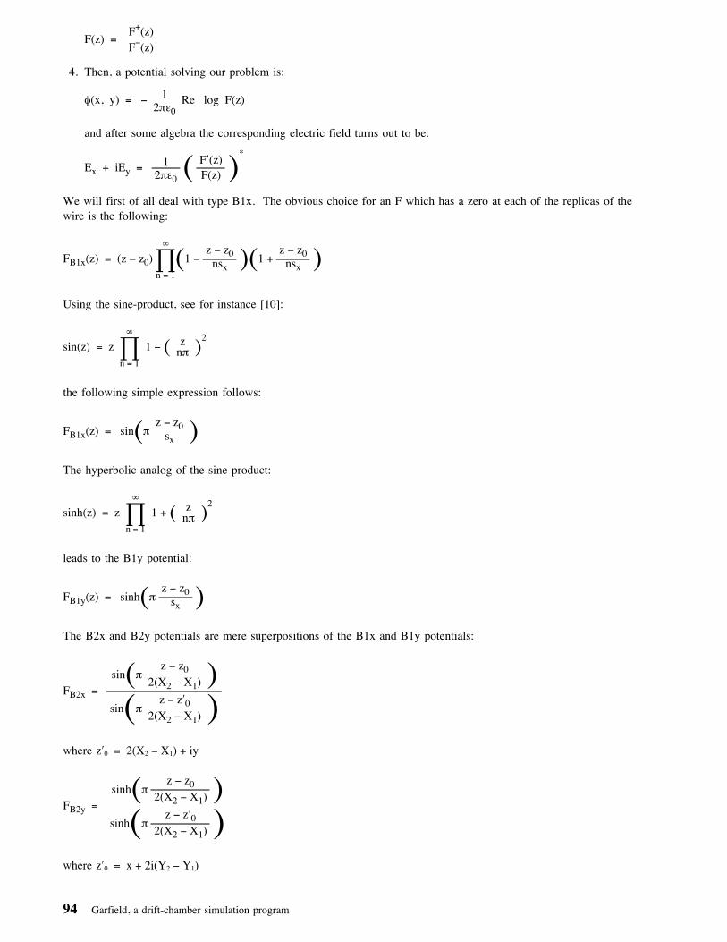
F(z) =F+(z) F−(z)

4. Then, a potential solving our problem is:

φ(x, y) = − 12πε0

Re log F(z)

and after some algebra the corresponding electric field turns out to be:

Ex + iEy = 12πε0 (

F′(z)F(z) )

*

We will first of all deal with type B1x. The obvious choice for an F which has a zero at each of the replicas of thewire is the following:

FB1x(z) = (z − z0)∏∞

n = 1(1 −

z − z0nsx )(1 +

z − z0nsx )

Using the sine-product, see for instance [10]:

sin(z) = z ∏∞

n = 1

1 − ( znπ )

2

the following simple expression follows:

FB1x(z) = sin(π z − z0sx )

The hyperbolic analog of the sine-product:

sinh(z) = z ∏∞

n = 1

1 + ( znπ )

2

leads to the B1y potential:

FB1y(z) = sinh(π z − z0sx )

The B2x and B2y potentials are mere superpositions of the B1x and B1y potentials:

FB2x =sin(π

z − z02(X2 − X1) )

sin(πz − z′0

2(X2 − X1) ) where z′0 = 2(X2 − X1) + iy

FB2y =sinh(π

z − z02(X2 − X1) )

sinh(πz − z′0

2(X2 − X1) ) where z′0 = x + 2i(Y2 − Y1)


4.1.5 Electrostatic field of a doubly periodic wire array(Contributed by G. A. Erskine)

4.1.5.1 Specification of the arrayWe consider a doubly periodic array of thin wires, the array consisting of replicas of a basic rectangular celldefined by 0 ≤ x ≤ sx, 0 ≤ y ≤ sy. This cell contains n wires, where wire j is characterised by:

PositionRadiusPotential

...

...

...

zj = xj + iyj,rj,

Vj.

Wires identical to wire j (j=1, 2, ... , n) are situated at:

zj + λsx + iμsy (λ, μ = 0, ± 1, ± 2, ...).

4.1.5.2 The thin-wire potential approximationWe shall obtain a potential function V(z) which satisfies the following conditions:

∂2V(z)

∂x2+

∂2V(z)

∂y2= 0,

z ≠ zj, j = ± 1, ± 2, ... , ± n. (1)

V(zk + rkeiφ) = Vk + o(rk), 0 ≤ φ ≤ 2π, k = 1, 2, ... , n. (2)

V(z + sx) = V(z), 'for all z.' (3)

V(z + isy) = V(z), 'for all z.' (4)

The exact potential function would be defined by the same conditions without any term o(rk) on the right-hand sideof (2). To simplify the formulae, electrostatic units are used.

We define V(z) = Re W(z) where

W(z) = ∑n

j = 1

qj { − 2 log ϑ1[ πsx

(z − zj), e−πsy/sx] + i 4πsxsy

yjz} + c (5)

with the theta function ϑ1 [11] defined by

ϑ1(ζ, p) = 2p1/4 ∑∞

m = 0

( −1)mpm(m + 1) sin(2m + 1) ζ, (6)

and with the n+1 real constants qj (j=1,2, ... ,n) and c determined by the system of equations

∑n

j = 1{ − 2 log | ϑ1[ π

sx(zi − zj), e−πsy/sx] | −

4πyiyjsxsy } qj + c = Vi, (i = 1, 2, ... , n), (7)


∑n

j = 1

qj = 0. (8)

In (7) first line we use the convention that, for the terms with i = j,

ϑ1[ πsx

(zi − zj), p] =πrisx

ϑ′1(0, p)

=πrisx

2p1/4 ∑∞

m = 0

( −1)m (2m + 1) pm(m + 1)(9)

The coefficient qj in (5) is the charge per unit length on wire j.

Condition (1) is satisfied because V(z) is the real part of a function (5) which is analytic everywhere except at thepoints zj (j=1,2, ... ,n). Condition (2) follows from (7) and (9). Condition (3) is an immediate consequence of (5)and (6).

To show that condition (4) is satisfied, define

wj(z) = − 2 log ϑ1[ πsx

(z − zj), e−πsy/sx] + i 4πsxsy

yjz.

Then, from the quasi-periodicity of the function ϑ1 [12], neglecting integral multiples of 2πi,

wj(z + isy) = wj(z) + i4πz − xj

sx− 2π

sysx

,

and hence

Re wj(z + isy) = Re wj(z) − 2πsx

(2y + sy)

Therefore, using (8),

Re W(z + isy) = Re ∑n

j = 1 qj wj(z + isy) + c

= Re ∑n

j = 1 qj wj(z) + c

= Re W(z).

4.1.5.3 Alternative expression for the thin-wire potentialBy considering the array obtained by rotating the original array through 90�, we see that the real part of the func-tion obtained from W(z) by replacing z by iz, zj by izj (j=1,2, ... ,n), and interchanging sx and sy, also satisfies theconditions (1) through (4). We thus obtain the alternative expression:

W(z) = ∑n

j = 1

qj { −2 log ϑ1[ iπsy

(z − zj), e−πsx/sy] − 4πsxsy

xjz} + c, (10)

where qj (j=1,2, ... , n) and c are determined by

∑n

j = 1{ − 2 log | ϑ1[ iπ

sy(zi − zj), e−πsx/sy] | −

4πxixjsxsy } qj + c = Vi, (i = 1, 2, ... , n), (11)


∑n

j = 1

qj = 0. (12)

The parameter p in the series (6) has the value e−πsy/sx when the expression (5) is used for W(z), and the value e−πsx/sy

when expression (10) is used. We therefore adopt the following rule:

If sx ≤ sy, compute W(z) from (5).If sx > sy, compute W(z) from (10).

This rule ensures that, for all values of sx and sy, we have p ≤ e−π = 0.043....

4.1.5.4 Field intensityThe components (Ex, Ey) of the electrostatic field intensity vector at z are given by:

Ex = − ∂V∂x

= − Re W′(z),

Ey = − ∂V∂y

= + Im W′(z),

where, depending upon whether we use (5) or (10) for W(z),

W′(z) = ∑n

j = 1

qj{ − 2πsx

ϑ′1[ πsx

(z − zj), e−πsy/sx]

ϑ1[ πsx

(z − zj), e−πsy/sx]+ i 4π

sxsyyj}

or

W′(z) = ∑n

j = 1

qj{ − i 2πsy

ϑ′1[ iπsy

(z − zj), e−πsx/sy]

ϑ1[ iπsy

(z − zj), e−πsx/sy]− 4π

sxsyxj}.

4.1.5.5 Periodic wire array between parallel electrodesThe complex potential of an array of wires which is periodic in the direction of one of the axes, and is bounded bytwo parallel zero-potential planes, is identical (in the region between the planes) to that of a doubly periodic arraywhose basic cell contains the original wires together with their reflections (with reversed sign for the wire potential)in one of the planes. If the planes are not at zero potential it is merely necessary to add a term linear in z.

Consider an array consisting of replicas in the x-direction of a group of n wires lying between zero-potential planessituated at y = Y1 and y = Y2. Let the wire positions be zj and the wire potentials Vj (j = 1, 2, ... , n), and let thex-periodicity be sx. If z is the complex conjugate of z, the reflection z′j of zj in the plane y = Y1 is given by

z′j = zj + i 2 Y1.

We now define a y-periodicity

sy = 2 (Y2 − Y1),

and consider the doubly periodic array with periods (sx, sy) consisting of replicas of a basic cell (enclosed by thebroken line in Figure 22 on page 98) containing 2n wires:


Figure 22. Periodic wire array between grounded parallel planes

Position

zj

z′j

Potential

Vj

− Vj

Charge

qj

− qj

From the symmetry of the positive and negative charges with respect to each of the planes y = Y1 and y = Y2

(Figure 22 ) it follows that these planes are at zero potential, and hence that the field of the doubly periodic arrayis the same as that of the original array. Using (5) and (10) respectively, we obtain the following expressions forthe complex potential:

Case 1. sx ≤ 2 (Y2 − Y1).

W(z) = ∑n

j = 1

qj{wa(z − zj) − wa(z − z′j) + i 8πsxsy

(yj − Y1) z}, (13)

where


wa(z) = −2 log ϑ1[ πzsx

, e−πsy/sx]. (14)

Case 2. sx > 2 (Y2 − Y1).

W(z) = ∑n

j = 1

qj{wb(z − zj) − wb(z − z′j)}, (15)

where

wb(z) = −2 log ϑ1[ iπzsy

, e−πsx/sy]. (16)

In both cases the qj are determined by the system of linear equations

∑n

j = 1

{ Re W(zi)}qj = Vi, (i = 1, 2, ... , n), (17)

where the convention defined by (9) is used for the terms with i = j.

Note that the sum ∑ (qj + q′j) of the 2n charges in the unit cell of the doubly periodic array is equal to zero, but thatthe sum ∑qj of the n physical charges is not necessarily equal to zero.

If, instead of being at zero potential, the planes y = Y1 and y = Y2 are at potentials v1 and v2 respectively, it isnecessary to add to the complex potential W(z) a term representing the superimposed uniform field, namely

(Y2v1 − Y1v2) + i (v1 − v2) zY2 − Y1

.

[Expressions equivalent to (13) through (16) were obtained by Buchholz [13] by direct summation of the contrib-utions of the individual wires and of their multiple reflections in the planes.]

4.1.5.6 Wire array inside a rectangular tubeWe consider n wires with positions zj and potentials Vj, (j = 1, 2, ... , n) lying inside a rectangular zero-potentialtube defined by X1 ≤ x ≤ X2, Y1 ≤ y ≤ Y2. The complex potential inside the tube is the same as that of atwo-dimensional periodic array of image charges having the symmetry shown in Figure 23 on page 100. Theperiods of this two-dimensional array are

sx = 2 (X2 − X1), sy = 2 (Y2 − Y1),

and the basic cell (enclosed by the broken line in Figure 23 on page 100) contains 4n wires:

Position

z(0)j = zj

z(1)j = zj + i2Y1

z(2)j = − zj + 2(X1 + iY1)

z(3)j = − zj + 2X1

Potential

Vj− Vj

Vj− Vj

Charge

qj− qj

qj− qj

Description

Physical wireReflection in the line y = Y1Reflection in the point X1 + iY1Reflection in the line x = X1

On defining, in terms of (14) and (16),

w(z) = wa(z) if X2 − X1 ≤ Y2 − Y1,w(z) = wb(z) if X2 − X1 > Y2 − Y1,


Figure 23. Wire array in a grounded rectangular tube

we obtain the required complex potential:

W(z) = ∑n

j = 1

qj {w(z − z(0)j ) − w(z − z(1)

j ) + w(z − z(2)j ) − w(z − z(3)

j )}, (18)

where the qj are determined by a system of linear equations (17) in which W(z) is computed from (18).

4.1.5.7 Computational considerationsBecause the expressions for W(z) either assume the relation ∑qj = 0 or depend only on the ratio of two ϑ1 func-tions, the constant 2 p1/4 in (6) makes no contribution. The series which need to be evaluated numerically aretherefore of the form

∑∞

m = 0

( −1)m pm(m + 1) sin(2m + 1)ζ [for W and W′], (19)

∑∞

m = 0

( −1)m (2m + 1) pm(m + 1) cos(2m + 1)ζ [for W′ only], (20)


where

p = e−πsy/sx,

p = e−πsx/sy,

ζ = πsx

(z − zj)

ζ = iπsy

(z − zj)

when sx ≤ sy,

when sx > sy.

If terms with m ≥ M are neglected when evaluating (19), the relative error in the sum is bounded approximately by

ρM = pM(M + 1) |

sin(2M + 1)ζsin ζ |

≤ (2M + 1) pM(M + 1) e2M|Im ζ|.

Assuming, as we may without loss of generality, that |x − xj| ≤ sx and |y − yj| ≤ sy, we find for both (5) and (10)that e|Imζ| ≤ 1/p. Hence,

ρM ≤ (2M + 1) pM(M − 1)

≤ (2M + 1) e−πM(M − 1).

In the same way, we may show that the relative error resulting from the neglect of terms with m ≥ M in theevaluation of (20) is bounded approximately by σM = (2M + 1) ρM. Setting M = 3, and using p ≤ e−π,

ρ3 ≤ 4.6 × 10−8.

σ3 ≤ 3.2 × 10−7.

Therefore, for practical computation, the expressions to be evaluated are:

sin ζ − p2 sin 3ζ + p6 sin 5ζ

cos ζ − 3p2 cos 3ζ + 5p6 cos 5ζ

[for W and W′],

[for W′ only].

To reduce the number of evaluations of sines and cosines of complex argument, we make use of the summationalgorithm [14], which in the present case takes the following form:

1. To evaluate Sn = ∑n

m = 0am sin(2m + 1)ζ:

s = sin ζα = 2 − 4s2 [ = 2 cos 2ζ]un = anun − 1 = an − 1 + αanfor j = n − 2 ( −1) 0 do uj = aj + αuj + 1 − uj + 2Sn = (u0 + u1) s

2. To evaluate Cn = ∑n

m = 0bm cos(2m + 1)ζ:

c = cos ζα = 4c2 − 2 [ = 2 cos 2ζ]un = bnun − 1 = bn − 1 + αbnfor j = n − 2 ( −1) 0 do uj = bj + αuj + 1 − uj + 2Cn = (u0 − u1) c


4.1.6 Isolated charges in a tube (type D1)Isolated charges in a tube are handled by conformally mapping the charge onto the centre of the tube using thefunction:

z → 1r

z − z0

1 − zz0/r2

After that, the type A potentials are applied.

4.1.7 Ring of charges in a tube (type D2)A ring of charges in a tube is dealt with using the conformal mapping

z → 1rn

zn − zn0

1 − (zz0/r2)n

provided z0 ≠ 0, otherwise the mapping for the D1 potential is used. The presence of two different potentials in thesame cell makes that the capacitance matrix can be asymmetric.

4.1.8 The capacitance equations, boundary conditions

The equations to be solved to find the wire charges are known as capacitance equations, they are obtained byexpressing the (known) potential of wire i in the (unknown) charges per unit length qj on the wires j = 1 to n.

The equipotential planes can be treated as if they were grounded if the linear potential Vplanes generated by theplanes alone is subtracted from all wire-potentials before the charges are calculated and added separately when thepotential and electrostatic field are evaluated. The equipotential planes are assumed to be grounded in the rest ofthis chapter.

Explicit charge calculations for equipotential planes may be avoided if (multiple) mirror charges are introduced.See Figure 21 on page 93 for their positions (&cdot. = original wire and even mirror images, × = odd image).

The sum of all charges should always be zero (the energy of the electric field would be infinite). If there is at leastone equipotential plane, the sum of all charges is automatically zero: the charges and mirror charges cancel. Thereference potential is set equal to zero in this case. The freedom to choose a reference potential can be exploitedwhen planes are absent. To find the charges, we therefore have to solve the following equations:

Vi = ∑nwires

j = 1

C−1ij qj + Vplanes(z) + Vreference ∑

wires + mirror wires

qj = 0

where |qjC−1

are the charges to be foundis the inverted capacitance matrix

Making use of the expressions earlier on in this chapter, the elements of the capacitance matrix can be written as:

C−1ij ≡ [− 1

2πε0Re log F(zi − zj)

− 12πε0

Re log (di limz → 0

F(z)z )

(i ≠ j)

(i=j)

and where F is a complex entire function such that

Re log F(z) = φ(z)


Once the charges per unit length are known, the potential at z can be evaluated from the formula:

V(z) = ∑nwires

j = 1

qjφ(z − zj) + Vplanes(z) + Vreference

4.1.9 Cylindrical geometry, internal coordinatesThis version of the program can perform some computations on certain types of cells which are more convenientlydescribed in polar coordinates for instance because of the presence of a circular plane. The program handles suchcells by transforming the polar coordinates to internal coordinates (ρ, φ) related to (x,y) via the conformal mapping(see for instance [15] for details):

(x, y) = e(ρ, φ) = (r cos φ, r sin φ) (21)

which translates circles into lines at constant ρ and radial lines into lines at constant φ. Radial symmetry in thenormal sense cannot be handled this way because this symmetry is absent in the internal coordinates (ρ is not linearin r). A slightly subtle point is the boundary condition at + π and − π if the cell does not have a φ periodicity. Theproper way to handle this is to impose a cyclic φ boundary condition with period 2π in the internal coordinates. 2πperiod in polar cells) Circular and radial planes and also symmetry in φ do not present problems. All calculationscan be performed using the normal routines, transforming to polar coordinates when plotting.

The transformation properties of some common geometrical objects can easily be derived using the transformationlaw (21):

scalars Scalars are, by definition, invariant.

Example: the electrostatic potential.

local vectors Local vectors behave like infinitesimal transformation, not like coordinates:

(dxdy) = eρ(cos φ

sin φ− sin φ

cos φ)(dρdφ)

Example: the drift-velocity.

co-vectors Co-vectors are derivatives of a scalar, it follows that they transform according to:

(∂x∂y) = e−ρ( cos φ

− sin φsin φcos φ)(∂ρ

∂φ)Example: the components of the electrostatic field. The expression in terms of polar coordinates issomewhat simpler:

Er, polar =Eρ, internal

r

Eφ, polar =Eφ, internal

r

axial vectors Of course the concept of an axial vector is weird in two-dimensional space. Embedding our two-dimensional space in a three-dimensional space, it makes sense to speak about an axial vector parallelwith the z-axis. We will call A an axial vector in this sense if

∀ vectors V: V × A is a co-vector

With this definition, the transformation of an axial vector simply reads:

Aζ = e2ρ Az

Example: a magnetic field parallel to the z-axis.

inner products Inner products of vectors and co-vectors are as usual scalars.

Example: the product encountered in the signal calculations.


4.1.10 Zeros of the electric fieldThe points where E = 0 is satisfied are the natural counterparts of the singularities at the wire positions and as suchplay a key role in the understanding of the behaviour of drifting particles in the chamber. Wires (and their mirrorimages) are the end points of the drift-lines whereas zeros are bifurcation points in the drift-field. It follows thatthe drift-lines from these points delimit the various acceptance regions. It should be noted on the outset that lim-iting oneself to the no-B case is not a true constraint since the drift-velocity vector is zero wherever E is zero, nomatter the B field (see Section 4.3 on page 110).

4.1.10.1 The saddle shape of the zerosE has a saddle point at its zeros owing to the harmonicity of the potential, as can be seen from a Taylor-expansionaround the zero:

(ExEy) = −( ∂2V

∂x2

∂2V∂x∂y

∂2V∂y∂x

∂2V

∂y2 )(δxδy) + ...

Assuming V satisfies the usual regularity conditions and using the harmonicity of V, one obtains after rotating overan angle

tan φ = ∂2V

∂x2/ ∂2V

∂x∂y

a diagonal form:

(EuEv) = − (λ

00

− λ) (δuδv) + ...

where λ is some (in the interesting case) non-zero number. The above treatment is valid for first order zeros, whichare certainly the only ones one meets in practice; it would be interesting to investigate the existence of higher orderzeros though.

The saddle shape can easily be inferred from this formula. An immediate -and important- consequence of thissimple fact is that the argument of E (i.e. the angle of the E vector) changes by −2π over one full counter-clockwiseloop around the saddle point. This is in marked contrast to wires where the argument changes by +2π.

4.1.10.2 The principle of the argumentThe principle of the argument is a convenient tool for counting the number of zeros and singularities (or poles) of acomplex analytic function inside a given area. It simply states that for a closed loop γ and an meromorphic func-tion f which has simple zeros and simple poles none of which lie on γ:

Δγ Arg f = 2π(number of zeros − number of poles)

This is not the most general phrasing of the theorem but it is adequate for our purposes (see [16] for a proof).Recall that E (complex version) is not a meromorphic function but the complex conjugate of one that is. Onemerely has to change the sign of the change in argument to compensate for this. Hence, we find that:

Δγ Arg E = 2π(number of wires − number of zeros)

4.1.10.3 Locating zerosThe principle of the argument can directly be applied to obtain via bisection regions that contain precisely one zero.The program uses a random search inside these areas to find good starting points and then steps towards the zeroswith a first (!) order stepping method that assumes a saddle shape; higher order methods, no matter how sophisti-cated, are inevitably inefficient.


4.1.11 Magnetic field calculationThe program does not contain routines for detailed magnetic field calculation; they may be added by the userhowever. The magnetic field routines the program supplies, are adequate for linear magnetic fields even if thedifference in magnetic susceptibility between the wires and the gas is to be taken into account. The distortion iscalculated from the formulae [17]:

Bx(x, y) = B0x + αB0

xy∑wires

ri2

di4 { + ( (x − xi)

2 − (y − yi)2) cos φ + 2(x − xi)(y − yi) sin φ}

By(x, y) = B0y + αB0

xy∑wires

ri2

di4 { − 2(x − xi)(y − yi) cos φ + ((x − xi)

2 − (y − yi)2) sin φ}

Bz(x, y) = B 0z

where|B0

x = x-component of the undisturbed magnetic field,

B0y = y-component of the undisturbed magnetic field,

B0z = z-component of the undisturbed magnetic field,

B0xy = √B02

x + B02

y ,

φ = angle of the magnetic field vector to the x-axis,

α =μwires − μgas

μwires + μgas,

μwires = magnetic susceptibility of the wires,μgas = magnetic susceptibility of the gas,

ri = radius of wire i,di = distance from (x, y) to (xi, yi).

These formulae are valid outside the wires, which is the region of interest. The program will correctly calculate thefield inside the wires as well.

4.2 Mixing gassesThe method used in Garfield to calculate the drift velocity and diffusion in gas mixtures, has been taken from thework of G. Schultz and J. Gresser [2].

The outline of this method is as follows: F(ε) represents the energy distribution function of electrons under theinfluence of an electric field E in the gas under consideration. F(ε) is decomposed in a series of Legendrepolynomials around the axis of the electric field and only the first two terms, F0(ε) and F1(ε) are kept. Using thetransport equations, one can express F1(ε) in terms of F0(ε). Under certain assumptions on inelastic collisions andexcitation processes, one can derive the following relation:

F0(ε) = C√ε e− ∫ε

0

3Λ(ε′)ε′dε′

(El(ε′))2 + 3Λ(ε′)ε′kBT

where C is a normalisation constant, Λ(ε) is the fraction of the energy lost by an electron during a collision with agas atom or molecule and l(ε) is the mean free path of electrons. The mean free path is inversely proportional tothe cross section, σ.

When mixing gasses, one uses the following effective values for the mean free path and the energy loss fraction:


σ = ∑i

fiσi

σΛ = ∑i

fiσiΛi

The drift velocity and diffusion are written as follows:

wdrift = 2 3

E√qe

2me ∫∞

0dε (εl′(ε) + l(ε)) F0(ε)

D = 1 3 ∫

∞

0dε l(ε)√ 2ε

meF0(ε)

The input parameters for these calculations, the cross section and the energy loss fraction, have been provided byFabio Sauli and Anna Peisert:

GasArgon (Ar)

First ionisation level15.759 eV

Parametrised range0.3 ≤ ε ≤ 11.5 eV

OriginWircha (J.Fehlmann)

Argon: energy loss Argon: cross section

GasMethane (CH4)


Parametrised range0.3 ≤ ε ≤ 8 eV

OriginFabio Sauli & AnnaPeisert

Methane: energy loss Methane: cross section


GasNeon (Ne)




Neon: energy loss Neon: cross section

GasIsobutane (C4H10)




Isobutane: energy loss Isobutane: cross section

GasCarbon dioxide(CO2)




Carbon dioxide: energy loss Carbon dioxide: cross section


GasHelium (He)




Helium: energy loss Helium: cross section

GasEthane (C2H6)




Ethane: energy loss Ethane: cross section

GasNitrogen (N)




Nitrogen: energy loss Nitrogen: cross section


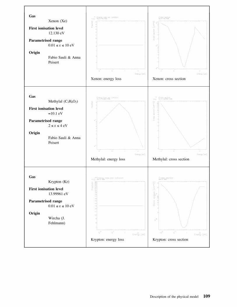
GasXenon (Xe)




Xenon: energy loss Xenon: cross section

GasMethylal (C3H8O2)

First ionisation level≈10.1 eV

Parametrised range2 ≤ ε ≤ 4 eV


Methylal: energy loss Methylal: cross section

GasKrypton (Kr)




Krypton: energy loss Krypton: cross section


GasAmmonia (NH3)

First ionisation level≈10.16 eV



Methylal: energy loss Methylal: cross section

4.3 Motion of electrons and ionsThis section briefly recalls the equations of motion for electrons and ions in a gas and the numerical method usedby Garfield to solve them. Two of the less straight-forward applications of drift-line calculation, x(t)-correlationand arrival time distributions, are dealt with in more detail.

4.3.1 The equation of motionThe drift-velocity of both electrons and ions is assumed to be determined entirely by the electric and magnetic fieldat their current position. This is justified by the short mean free path as compared to the length of normal drift-lines. The equation of motion is therefore a set of 2 coupled first order differential equations:

(x., y

.) = v

→drift (x, y)

v→

drift takes, in the absence of a magnetic field, the simple form:

v→

drift(x, y) = E→

(x, y) μ(E)

where μ(E) is called the mobility.

The drift-velocity of a particle under the influence of both a magnetic and an electric field is given by:

v→

drift =μ

1 + ω2τ2 (E→

+ E→

× B→

|B|ωτ +

(E→

• B→) B→

B2ω2τ2)

where |ω = the cyclotron frequency,

τ = the average time between atomic collisions,E and B are to be evaluated at (x,y).

This formula is proven in [18]. It might be appropriate to note that ωτ equals μ|B→

| in this approximation. Hencethe third term (or the second if E

→ and B

→ happen to be orthogonal) will dominate in the case of electrons, for which

usually ωτ > > 1. For ions on the other hand, where typically ωτ < 1, the first term tends to be largest.

The Lorentz angle calculated from the above formula does not describe the experimental data very well.


The mobility μ has been tabulated for many gasses as a function of E/p (p is the pressure, the mobility scalesroughly in E/p). The tables are interpolated using cubic splines [19] or Newton polynomials via the CERN libraryroutine DIVDIF (E105).

4.3.2 Numerical solution of the equation of motionThe differential equation of motion is solved numerically using a 2nd-3rd order Runge-Kutta-Fehlberg (RKF) method[20], which adjusts the step-size such that the overall accuracy increases, while the amount of CPU time usedremains comparatively low.

The method works as follows. The drift-velocity at the initial positionz0, v→

drift(z0) is used to obtain an initial step-size (in time) using:

δt = ε

|v→

drift(z0)|

where ε is the absolute integration accuracy

This estimate of the step-size is usually on the safe side, but this is harmless because its value can increase rapidly.Next, the algorithm repeatedly makes a second and a third order estimate of the next step to take from the currentpoint z, initially z�:

Δv→

I = ∑2

k = 0

CkI v→

k

Δv→

II = ∑3

k = 0

CkII v→

k

where

v→

k = v→

drift(z + δt ∑k − 1

l = 0

βklv→

l)The coefficients, which have been chosen such that one field evaluation from the previous cycle can be reused, canbe found in the reference. The difference between the two estimates is used to update the step-size:

δtnew = √ε δtold

|Δv→

I − Δv→

II|

After each step, a guess is made of the most likely target wire. Only wires charged oppositely to the particle areconsidered. During the evaluation of the v

→k for the next step, checks are made to ensure that none of the 'sensing'

points lies at the other side of the target wire or at the other side of a plane. If the target wire has been crossed,another algorithm for stepping towards a wire takes over. If a plane has been crossed, a simple linear step towardsthe surface is made. After each step, a check is made to ensure that the particle is still within the user-defineddrift-area; if it is not, the last step is trimmed. A few other conditions, such as exceeding the maximum number ofsteps (MXLIST), stopping and returning, may cause early abandoning of the calculations at this stage. Also aftereach step, the wire closest to which the particle passed by is determined (this may, but need not, be the target wire).If the minimum distance is smaller than the radius times a user-defined multiplication factor (TRAP), the wire isconsidered to be hit and the drift-line is terminated by the wire algorithm.

Terminating a drift-line once the target wire is known, is a great deal simpler than free drift-line calculation. It ishowever surprisingly important to do the final stepping accurately because the success of for instance the x(t) calcu-lation hinges on a better than 0.1 % accuracy of the total drift-time estimate.


As a first step, the amount of time needed to reach the wire from the current last point, is estimated. A tentativestep of this length is made of which the accuracy is tested by means of an intermediate point. If not satisfactory,the step-length is repeatedly halved. A step is truncated if it would end up insider the wire. The method terminatesif either of two conditions is satisfied: the particle moves away from the wire (for instance if the wire has a largedipole moment) or if the last step reaches the wire-surface. The time is integrated using the Simpson rule, makinguse of the fact that the field near the surface is roughly logarithmic. This method emphasises accurate timing andneglects accurate positional tracking, this is justified by the circumstance that the path is almost straight near thewires.

The routines involved in calculating drift-lines communicate with little more than a status code (ISTAT) which tellson which wire the drift-line ends or whether it ended on a plane etc. The routines asking for drift-lines usuallyexamine the code. The meaning of the various values is explained in Section 6.3 on page 129, under the headingDLCSTA and DLCALC.

The equal arrival time points are interpolated on the drift-lines, using third-order splines.

4.3.3 Calculation of x(t)-relationsThe x(t)-correlation for a wire at (xwire, ywire) is the relation between x and the minimum time an electron starting ona line through (x, ywire) at an angle φ to the y-axis needs to reach the wire. x(t)-Relations are used in the offlineevent reconstruction in order to correlate the measured time of a hit with a position in the chamber. The x(t)-correlations calculated by Garfield should merely be seen as a rough indication, not as immediate input to a recon-struction program, even though the algorithm can usually achieve a better than 0.1 % internal consistency if theparameters have been adjusted with care. The main reason is that the drift-velocity is usually not known withenough accuracy, something no simulation program can correct for ! T0 and slope corrections are almost certainlyneeded.

The algorithm used by Garfield for calculating x(t)-correlations is the following.

• Drift-lines are calculated starting from the wire surface between the user-specified limiting angles. Each ofthese drift-lines is interpolated on all of the x points for which a t has been requested. For each x a table ismaintained of the 3 shortest interpolated times.

• The algorithm recalculates the drift-line corresponding with the shortest time. The algorithm stops at this pointif three data-points for a given x have been obtained already and the relative difference between the parabolicminimum of these 3 points and the recalculated value does not exceed ε. The algorithm stops also if nooptimisation has been requested.

• Otherwise, additional data-points are sought for the x for which less than 3 points have been found so far.None of these 3 points is left in the interpolated state.

• The last stage is a parabolic minimisation in which a new optimum replaces the worst of the 3 data-points untilconvergence is achieved:

|tparabolic − tminimal| < ε|tparabolic + tbest|

The calculations are abandoned if no convergence can be achieved within the user-specified maximum numberof iterations. Checks are made to ensure that the stationary point of the parabola is not a maximum.

The parameter ε can be set by the user via the PRECISION keyword.

4.4 Signal simulationThe signal on the sense wires which results from the passage of a charged particle through the chamber, is simu-lated in Garfield by simple Monte-Carlo techniques. Three main steps may be distinguished in this simulation:

4.4.1 Track generationThe path of the particle is part of the input to the program.


4.4.1.1 Cluster positionsWe assume that the energy of the charged particle is much larger than energy lost on average in collisions withgas-molecules. Hence, the distance between 2 clusters is in excellent approximation independent of the location ofthe other clusters. The number of clusters per unit length is therefore Poisson distributed or equivalently, the dis-tance between two clusters is exponentially distributed:

f(d) = e− nd

where n is the average number of clusters per unit length.

4.4.1.2 The cluster-size distributionIf the cluster-size distribution has been measured, it is of course preferable to use it. However the distribution isvery often not available and one has to resort to some more or less sophisticated means of calculating it fromknown parameters. This section explains the fairly simple method this program puts at your disposal.

According to Landau the energy deposited by a charged particle passing through some material, is given by thedistribution (the so-called Landau distribution):

fLandau(λ) = 12πi ∫

c + i ∞

c − i ∞es log(s) + sλds

= L−1es log(s)

where |λ: dimensionless, linear in the energy,L−1: the inverse Laplace transform

In our case the energy is deposited in clusters rather than continuously as required for the Landau distribution. Weshould therefore draw the required energies from a modified Landau distribution fLandau

n (λ) which has the propertythat the sum of n numbers drawn from this distribution is Landau distributed:

f Landau *

n

n = fLandau

(The "*" stands for a multiple convolution.) Since the Landau distribution takes the form of an inverse Laplacetransform, the relation between fLandau

n and fLandau is:

f Landaun (λ) = L−1e

s log(s)n

= 12πi ∫

c + i∞

c − i∞e

sn

log( sn

) + sn

( log(n) +λn)d( sn )

= n fLandau(nλ + log(n))

Hence the distribution function of the primary cluster-size reads in this simple approximation:

Psize(m) = nξ ∫

(m + 1) Epair

m Epair

fLandau(nE − Emostprob

ξ+ log(n))dE (22)

where|m: the actual cluster-size,Emostprob: the most probable energy loss per unit length,Epair: the energy required for one electron ion pair,ξ = K Z

Aρ, assuming the particle travels at the speed of light,

K: a numerical constant,A, Z: suitably weighed atomic number and nuclear charge,ρ: the density.


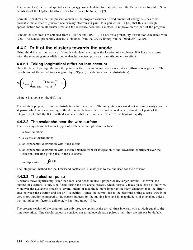
The parameter ξ can be interpreted as the energy loss calculated to first order with the Bethe-Bloch formula. Somedetails about the Laplace transforms can for instance be found in [21].

Formula (22) shows that the present version of the program assumes a fixed amount of energy Epair has to bepresent in the cluster to generate one primary electron-ion pair. It is pointed out in [22] that this is a roughapproximation for small cluster-sizes and the reference describes a method to improve on this part of the program.

Random cluster-sizes are obtained from HISRAN and HISPRE (V150) for a probability distribution calculated with(22). The Landau probability density is obtained from the CERN library routine DENLAN (G110).

4.4.2 Drift of the clusters towards the anodeUsing the drift-line routines, a drift-line is calculated starting at the location of the cluster. If it leads to a sensewire, the remaining steps (diffusion, avalanche, electron pulse and ion-tail) come into effect.

4.4.2.1 Taking longitudinal diffusion into accountOnly the time of passage through the points on the drift-line is uncertain since lateral diffusion is neglected. Thedistribution of the arrival times is given by ( N(μ, σ2) stands for a normal distribution):

N(tmean, ∫drift-line

σdiffusion(z)2

vdrift(z)2dz)

where z is a point on the drift-line

The addition property of normal distributions has been used. The integration is carried out in Simpson-style with astep-size which varies according to the difference between the first and second order estimates of parts of theintegral. Note that the RKF method guarantees that steps are small where ve is changing rapidly.

4.4.2.2 The avalanche near the wire-surfaceThe user may choose between 4 types of avalanche multiplication factors:

1. a fixed number;

2. a Gaussian distribution;

3. an exponential distribution with fixed mean;

4. an exponential distribution with a mean obtained from an integration of the Townsend coefficient over theelectron drift-line giving rise to the avalanche:

multiplication = e ∫α(z)dz

The integration method for the Townsend coefficient is analogous to the one used for the diffusion.

4.4.2.3 The electron pulseElectrons move significantly faster than ions, and hence induce a proportionally larger current. However, thenumber of electrons is only significant during the avalanche process, which normally takes place close to the wire.Moreover the avalanche process is several orders of magnitude more important in many chambers than the differ-ence between the electron and ion drift-velocities. Hence the current due to the electrons hitting a sense wire is ofvery short duration compared to the current induced by the moving ions and its magnitude is also smaller, unlessthe multiplication factor is deliberately kept low (about 10�).

The present version of the program can only produce spikes at the arrival time interval, with a width equal to thetime-resolution. One should seriously consider not to include electron pulses at all; they are left out by default.


4.4.3 Calculation of the ion-tailThe ions created during the avalanche account for a large fraction of the visible signal in drift-chamber experimentsand it is therefore appropriate that the currents they induce on the sense wires when drifting towards the cathodesare accurately calculated. This part of the signal is known as 'ion-tail'. The method used in this program isinspired by [23].

An exact expression for the induced charge λi may be obtained using the Green reciprocity equations [24, 25] tocalculate the induced charges; differentiation to time gives the induced current. Consider the following physicallyacceptable situations:

1. The configuration of interest to us:

charge of the ionpotential at the ions positioncharge on wire ipotential of wire i

Qion? (not relevant)

qi + λiVi

Note that the potential on the surface of wire i is unchanged as compared to the rest situation where the wirecharges are qi. The extra charge λi on the wires is assumed to be removed instantly.

2. In this configuration only wire j carries a charge, the other wires and the ion being uncharged.

charge of the ionpotential at the position of the ioncharge of wire jpotential of wire jcharge of wire i ≠ jpotential of wire i ≠ j

0qj φ(zion − zj)

qjqj φ(zj − zj)

0qj φ(zi − zj)

In both cases the reference potential and the potential due to the equipotential planes are assumed to have beensubtracted.

Applying the Green reciprocity equations and differentiating yields:

∑nwires

i = 1

λi φ(zj − zi) = − Qion φ(zion − zj)

∑wires

Ii φ(zj − zi) = Qion ε→

(zion − zj) • v→

ion

where|ε→

(z) = − ∇→φ(z),

v→

ion is the drift-velocity of the ion,

Ii =dλidt

, the induced current

Ii is therefore determined by a system of linear equations if the cell is not periodic.

If the cell is truely periodic however, the potential used for the field calculations is no longer applicable since,clearly, the signal on the replicas of a wire is different from the signal on the wire in the basic cell. Insteadpotentials which do not have true periodicities should be taken:

B1x B1y C2x C2y

→→→→

AAB2x B2y


The complexity of the equations to be solved is also considerably greater in the periodic case since we then havematrix convolution equations:

∑∞

m =−∞∑nwires

i = 1

Ii[m] φ(zj[n] − zi[m] ) = Qion ε→

(zion − zj[n] ) • v→

ion

where |zj[m] = zj + ms, s the periodicity of the cell,

Ii[m] is the induced current on the wire at zi + ms.

Similar equations hold for the doubly periodic case.

These equations are best solved by means of Fourier transforms, provided some care is taken to avoid aliasing andconvergence problems. [This is something to be done by the user in the present version of the program]. Indeed asolution to the above set of equations is:

Ii[n] = Qion ∑∞

m =−∞∑nwires

j = 1

F−1{F φ(zj[n] − zi[m])}−1 ε→

(zion − zj[n]) • v→

ion

where F is a forward Fourier transform and F−1 its inverse. It should be clear that especially the doubly periodiccase demands the manipulation of huge amounts of numbers, if a high degree of accuracy is needed.

Figure 24. Comparison of a measured and simulated signal. The simulated signal has been corrected for reflection and isfolded with the transfer function of the read-out electronics. (Courtesy Matthias Grosse Perdekamp [26].)

4.5 Evaluation of symbolic formulaeThe program frequently needs general expressions in terms of a set of variables. Although the user could in prin-ciple provide these relations as Fortran functions, it would be inconvenient to do so (the program has to be recom-piled and reloaded each time a formula is changed). It is for this reason that the program contains a set ofsubroutines capable of evaluating symbolic formulae.


Roughly speaking, each formula is translated into an instruction list (independent of the current value and type ofthe variables) which can be executed any number of times.

This section explains in detail how symbolic formulae are handled by the program. It also contains some guidelinesfor constructing formulae. Refer to Section 3.12.11 on page 87 to see how the instruction lists can be edited.

4.5.1 GuidelinesThe format of the formulae closely resembles Fortran, there are however a few differences:

• Not all Fortran functions are available and some intrinsic functions have a different name (see the table below),

• The data types recognised by these routines are: string, number, logical and histogram. No distinction is madebetween integers and reals and the Fortran data types DOUBLE PRECISION and COMPLEX are not known.

• Blanks are significant in such formulae as EXP X or SIN COS X, both of which are correct provided X is alegal variable. Blanks inside variable and function names should be avoided. On input, a blank is treated as aseparator and formulae which contain blanks are therefore split into pieces unless they have been put betweenquotes (both single and double quotes will do).

• Identifier names may be up to 10 characters long.

• Constants and constant intermediate results differing less than a fraction 10−4 (machines other than Cray) or 10−8

(Cray) from an already stored constant, are considered to be equal to that constant.

The symbol PI may be used in all formulae for π, e.g. to convert degrees into radians as input for the functionsSIN, COS and TAN.

The program tries to make instruction list which are fast. E.g. it will try to avoid repeated evaluation of identicalsubexpressions. The program will succeed only if the subexpressions look alike and it helps if you put thembetween brackets.

Fortran compiled functions execute up to 5 times faster than the corresponding instruction lists. In case you intendto make heavy use of functions, it might therefore be a better idea to modify the program. Alternatively you couldtry and make an optimised instruction list yourself, see Section 3.12.11 on page 87 on editing.

4.5.2 Details about the translation processFirst, each formula is translated by ALGPRE into a list of instructions (similar to the programming of a pocketcalculator). Then, each time ALGEXE is called, the variables in the formula are replaced by their values, theinstructions are carried out one by one (by ALGEX2) and the result(s) are passed to the calling subroutine.

The translation carried out by ALGPRE, is in fact a 4 step process:

1. The input string T is copied into a string S and an integer array P, during which the following substitutions aremade:

Table 4 (Page 1 of 3). Formula translation table. Translation of formulae

Input S P Notes

(, [ ( 0 Yes, square brackets are allowed !

), ] ) 0

constant R ≤ 0 See comments on step 3.

variable R >0 See comments on step 3.

TRUE R -1 Logical value TRUE.

FALSE R 0 Logical value FALSE.

+ O 1 Numbers: add, Logicals: or, Strings: concatenate.



Input S P Notes

- O 2 Numbers: subtract, Logicals: exclusive or.

* O 3 Numbers: multiply, Logicals: and.

/ O 4 Divide.

** O 5 For Arg1 > 0 or Arg2 integer.

= O 10 Numbers: |Arg1 − Arg2| < 10−5, Logicals: Arg1⇔Arg2.

#, < > , > < O 11 Numbers: |Arg1 − Arg2| > 10−5, Logicals: Arg1⇔/ Arg2.

< O 12 Returns TRUE if Arg1 < Arg2.

<=, =< O 13 Returns TRUE if Arg1 ≤ Arg2.

> O 14 Returns TRUE if Arg1 > Arg2.

>=, => O 15 Returns TRUE if Arg1 ≥ Arg2.

& O 16 Logical AND between logicals.

| O 17 Logical OR between logicals.

EXP F 1

LOG F -1 For Arg > 0.

SIN F 2

ARCSIN F -2 For |Arg| ≤ 1.

COS F 3

ARCCOS F -3 For |Arg| ≤ 1.

TAN F 4

ARCTAN F -4

ABS F 5

SQRT F -5 For Arg ≥ 0.

+ F 6 As a monadic function (e.g. +2.0).

- F -6 As a monadic function (e.g. -3.0).

SINH F 7

ARCSINH F -7 Not an intrinsic function.

COSH F 8

ARCCOSH F -8 For |Arg| ≥ 1, not intrinsic.

TANH F 9

ARCTANH F -9 For |Arg| ≤ 1, not intrinsic.

NOT F 10 NOT function, also hat and tilde.

ENTIER F 11 Entier function.

TRAILING F -11 ≡ Arg − Entier(Arg).

STRING F 12 Converts a number or logical to a string.

NUMBER F -12 Converts a string to a number.

SUM F 13 Sum of histogram contents.


Other symbols are ignored and an error message is issued. Note on powers: negative numbers can only beraised to powers that are (near) integer, the sign being negative for negative numbers to an odd power, even forother cases. Zero can be raised to any power larger than zero.

Example:

T =S =P =

$0

TANF4

( ( 0

SINF2

( ( 0

+F6

XR1

**O5

2R2

+O1

ABSF5

( ( 0

YR2

) )0

) )0

) )0

+O1

1R1

$0

(23)

At the same time, the balance of the brackets is checked. The formula is not accepted if unknown variable orfunction names have been used.

2. The string S is checked for illegal sequences of symbols, like functions without argument or * followed by /etc.

3. The string S and the array P are used to create the instruction list. This process identifies the deepest level,assigns the result to an element in REG, looks for the next deepest level etc.:

The order of precedence of the operators is established by the P-code except that arithmetic operators haveprecedence over comparisons, and comparisons have precedence over binary logical operators. Thus, anexpression like i = 5|i = 6 needs no brackets.

Each instruction is made up of 4 integers:

a. either a function-specification (code as in P) or an index in REG,

b. code for the operation (same as in P, 0=result, 6=function),

c. an index in REG,

d. the index in REG of the result or the index in the output array RES in case of a final result (both the firstand the second element are 0 in this case).


Input S P Notes

PRODUCT F 14 Product of histogram contents.

REFERENCE F 14 Reference to histogram.

RND_UNIFORM F -21 Uniform random number between 0 and 1

RND_GAUSS F -22 Gaussian random number, G(0, 1)

RND_EXP F -23 Exponential random number, mean 1

RND_LANDAU F -24 Landau random number

RND_POISSON F -25 Poisson random number

, $ 0 Separates formulae.

Table 5. Instruction list building. Substitutions made when building the instruction list

input output conditions

FR R Always

ROR) R) If not preceded by a higher precedence O

ROR$ R$ Idem

RORO RO idem, if the second O has lower precedence

(R) R Always


The array indices in 3a, 3c and 3d are identical to the code in P for constants and variables (except for func-tions and final results).

There are a few more instruction list codes which are recognised by both the instruction list execution routinesand the instruction list printing routine. They are not generated in the translation process as performed byALGPRE but can be used to construct loops, call procedures and to jump. Use the editor (Section 3.12.11 onpage 87) to enter them.

The array REG mentioned in the previous paragraph stores all constants, variables and intermediate results.The variables occupy the first n places from REG(1) onwards, n being the number of variables. Constants haveindices from -4 downwards, except 0, 1, 2 and π which are always kept in REG(0), REG(-1), REG(-2) andREG(-3). Constant intermediate results are stored 'below' the last constant appearing in the formula, non-constant intermediate results 'above' the last variable. Logicals are represented as 0 for FALSE and as 1 forTRUE.

All elements of the array REG have a type: string (code 1), number (code 2) or logical (code 3). The type ispropagated during the execution of an instruction list. The instruction list by itself has no data type informationand it may therefore be possible to execute one and the same list for different data types. For instance, A+Bwill work for strings, numbers and logicals, respectively carrying out a concatenation, an addition and an or.

4. The instruction list is simplified: constant expressions are evaluated, complementary functions and operators are(to some extent) removed, repeated evaluation of identical subexpressions is avoided etc. Most of these stepsare not performed when GOTO's occur. Finally unused constants (excluding 0, 1, 2 and π), auxiliary variablesand instructions are removed. The subroutine tells the calling routine which variables are effectively used.

Table 6. Additional instruction list codes. The instruction list execution routines recognises the following instructionswhich can be used to make control structures.

Function Ins(1) Ins(2) Ins(3) Ins(4) Notes

Return i -9 0 - If Ri = True Then leave procedure

Exit i -9 1 - If Ri = True Then leave procedure nest

Quit i -9 2 - If Ri = True Then leave program

Goto i 7 j - If Ri = True Go to instruction Rj

Argument 0 8 i j Argj : = Ri, modifiable

Argument 1 8 i j Argj : = Ri, not modifiable

Call i 9 j - Call Proci with j arguments

Table 7. Instruction list. This example shows the instruction list for formula (23).

Ins(1) Ins(2) Ins(3) Ins(4) Notes

6 6 1 5 +X → REG(5), 4 variables are assumed

5 6 2 6 ABS(Y) → REG(6)

5 5 -2 7 REG(5) → REG(7), REG(-2)=2

7 1 6 8 REG(7)+REG(6) → REG(8)

2 6 8 9 SIN(REG(8)) → REG(9)

4 6 9 10 TAN(REG(9)) → REG(10)

10 1 -1 11 REG(10)+1 → REG(11), REG(-1)=1

0 0 11 1 REG(11) is the first (and only) result


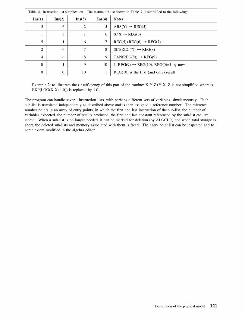
Example 2: to illustrate the (in)efficiency of this part of the routine: X-Y-Z+Y-X+Z is not simplified whereasEXP(LOG(X-X+1.0)) is replaced by 1.0.

The program can handle several instruction lists, with perhaps different sets of variables, simultaneously. Eachsub-list is translated independently as described above and is then assigned a reference number. The referencenumber points in an array of entry points, in which the first and last instruction of the sub-list, the number ofvariables expected, the number of results produced, the first and last constant referenced by the sub-list etc. arestored. When a sub-list is no longer needed, it can be marked for deletion (by ALGCLR) and when total storage isshort, the deleted sub-lists and memory associated with them is freed. The entry point list can be inspected and tosome extent modified in the algebra editor.

Table 8. Instruction list simplication. The instruction list shown in Table 7 is simplified to the following:

Ins(1) Ins(2) Ins(3) Ins(4) Notes

5 6 2 5 ABS(Y) → REG(5)

1 3 1 6 X*X → REG(6)

5 1 6 7 REG(5)+REG(6) → REG(7)

2 6 7 8 SIN(REG(7)) → REG(8)

4 6 8 9 TAN(REG(8)) → REG(9)

0 1 9 10 1+REG(9) → REG(10), REG(0)=1 by now !

0 0 10 1 REG(10) is the first (and only) result



5.0 Compiling the program

This chapter explains how an executable module can be made. The main steps in this process are:

• obtaining the source files;

• adapting explicit file locations to your installation;

• running YPATCHY to make a Fortran compile input file and perhaps to generate auxiliary files;

• compilation of the program, and of the help, message, command language definition, LSE and assembler files;

• linking the compiled (object) file with library routines,

Executable modules ready for use, are stored on many computers at CERN and outside.

5.1 Obtaining the source file

5.1.1 Distribution conditionsGarfield is distributed by the CERN Program Library Office following the general guidelines and conditions appliedto Program Library material. The text of the distribution conditions can be requested from:

CERN Program Library OfficeCERN-CN DivisionCH-1211 Geneva 23Switzerland

Tel: +41 22 767 4951Fax: +41 22 767 7155

EARN/Bitnet: CERNLIB@CERNVMDECnet: VXCERN::CERNLIB (node 22.19�)Internet: [email protected]

5.1.2 File locationThe program is distributed as a set of 2 files in Patchy format, one is a CARDS file and the other a CRADLE file.Both can also be found in the locations shown in Table 9.

5.1.3 Source file contentsThe source file as you receive it from CERN contains the components shown in Table 10 on page 124.

Table 9. File location. The current, past and future versions of the source file for Garfield can be found in the placeslisted in the table. The name shown is for the CARDS file, for the CRADLE file only the suffix is different:"cra" instead of "car".

Computer File location Access

CERNVM old: GARFIELD CAR on CERNLIB 301pro: GARFIELD CAR on CERNLIB 311new: GARFIELD CAR on CERNLIB 321

ftp from cernvm.cern.ch,IP address 128.141.2.4

VXCERN old: CERN:[OLD.SRC.CAR]GARFIELD.CARpro: CERN:[PRO.SRC.CAR]GARFIELD.CARnew: CERN:[NEW.SRC.CAR]GARFIELD.CAR

Decnet

Unix old: /cern/old/src/car/garfield.carpro: /cern/pro/src/car/garfield.carnew: /cern/new/src/car/garfield.car

-

Compiling the program 123

5.2 The YPATCHY stepRunning Patchy would normally be done by the make procedure described in Section 5.3 on page 126. One there-fore, in principle, does not need to understand the meaning of the various Patchy flags. Since modification of thePatchy cradle file is frequently needed however, details of the Patchy step are given here.

The Patchy step plays a key role in the compilation process. Not only does it serve to insert the common blocks, itis also the time a specific program version (computer, plotting package, interfaces) is chosen.

Choices are made depending on the settings of so-called Patchy switches which are in fact simply patch names.This program adheres to the convention that the switches of which the name starts on a *, are true patches in whichother switches are set. Such patches are called pilot patches because they are never used in +SELF statements.(+SELF statements are sort of IF directives to Patchy.) They do not contain Fortran. Thus, there is a fundamentaldifference between the switch *CMS and the switch CMS: the first selects CMS, NAG and GKS whereas the lattermerely stands for itself.

The correct choice of the target machine during the Patchy step is of importance. Although extensions to theFortran standard have been avoided, there are some on nearly all machines. In particular on VM/CMS, machinespecific calls are heavily used for file access.

The plotting package is normally chosen in one of the pilot patches but this choice can be overruled by the userusing the more specific switches listed below.

If the program size without arrays is too large, you may wish to exclude some sections from compilation. This isachieved by inserting +USE,P=< section >,T=INHIBIT cards as shown below.

Table 10. Source file contents. The Garfield source file contains the components listed below.

Name Relevant for Purpose Processing

- All computers Main program YPATCHY, Fortran. On Vax linkwith FIOPAT andGARFIELDCLD

FIOPAT.MAR Vax/VMS Alternate I/O library, seewriteup Z037,

MACRO

GARFIELDCLD.CLD Vax/VMS Command language defi-nition

SET COMMAND /OBJ

garfield.hlp All computers On-line help file %pack-help in Garfield

garfield.l Unix Introductory help file nroff -man catl/garfield.l >manl/garfield.l

GARFRUN.FOR Vax/VMS Front-end program Fortran, link withGARFRUNMSG

GARFRUNMSG.MSG Vax/VMS Message definitions forGARFRUN.FOR

MESSAGE

GARFRUN.HLP Vax/VMS Introductory help file LIBRARY/CR/HELP

GARFIELD.LSE Vax/VMS LSE template file LSE/NODISP/INIT=GARFIELD.LSE

GARFIELD EXEC VM Front-end exec optionally, REXXD

GARFMINI EXEC VM Minimal front-end exec none

GARFIELD PANEL VM Panels used byGARFIELD EXEC

none

GARFIELD SHLPCMS VM Introductory help file CONVHELP


Storage space allocation is largely static (i.e. there is no dynamic memory management on the numerical arrays);the array dimensions are fixed during the YPATCHY run. The program prints a message telling you which param-eter to increase when it hits the maximum size of an array. You may also wish to decrease some compilationparameters in order to reduce the storage space needed by the program. In both cases, a +REP,P=COMMONS,C=card has to be inserted in the cradle. The correct card numbers can be found in a YLIST listing of the program.Some care has to be exercised because the parameters are not completely independent; at present the program doesnot perform error checking on the consistency of the array dimensions.

Suggested Patchy cards are:

+EXE.+USE,< section name >,T=INHIBIT. (one per unused section)+REP,P=COMMONS,C= ... . (change array dimensions) PARAMETER(MXWIRE=2��)+USE,*< computer name >.+USE,*GARFIELD.

(correction cards, other options)+PAM. or +PAM,T=CARDS. (depends on PAM type)

(user decks if any)+QUIT.

The < computer name > can be APOLLO, CMS, CRAY, MVS, SUN or VAX. The flag *GARFIELD requests acompiler input file to be written with all sections of the program that were not explicitly de-selected by the user(+USE,< section name >,T=INHIBIT. cards).

The +USE,*< computer name >. cards refer to pilot patches which contain amongst others the Patchy switcheslisted below. You may use them directly if none of the *< computer name > patches suits you.

APOLLO To be used when compiling on an Apollo. A few Apollo extensions to Fortran-77 are used in non-critical parts of the program. Operating system SR10 is assumed.

AST (Effective only together with the VAX flag.) Enables control-C interception on a Vax. The routinestaking care of the interrupt handling have been written in Vax Fortran-77; they were kindly provided byCarlo Mekenkamp, Rijks Universiteit Leiden. The program runs perfectly well when this flag has beendisabled. When compiling with this flag, be sure you link with FIOPAT. The linker will scream thatthere are multiply defined symbols, this is normal since FIOPAT replaces the RTL I/O routines. Inter-rupt handling for other computers might be added as the need arises provided the expertise is available.

ATCGKS When this flag is enabled, Patchy assumes the program will be linked with ATC GKS.

CERN Enables calls to some packages, like NAG, which are not generally available outside CERN.

CMS To be used when compiling with VS-Fortran under VM/CMS. This switch is essential for proper func-tioning under CMS as explained above. Make sure a library routine equivalent to VMCMS is available.A skeleton of such a routine is provided in deck VMCMS, patch ROUTINES of the PAM file; theassembly language part of it has not been written by the author of Garfield. Garfield assumes in theroutine providing help a version 2 of VS Fortran.

CRAY To be used when compiling for a Cray computer. Debugging of the program has by now shifted to theCERN Cray XMP-48 and compilation with the cft77 compiler as well as loading with segldr workswell. The program has only be run under UNICOS. There are still some areas in the program to bechecked. A few CPU intensive routines are provided in vectorisable format.

DECGKS When this flag is enabled, Patchy assumes the program will be linked with DEC standard GKS. Theflag should only be selected in conjunction with the VAX flag.

DECS Use this flag when you intend to run on a DecStation or similar Unix workstation.

GTSGRAL Switch to be set if the program will be loaded with GTS-GRAL/GKS, default on all machines exceptSun. Since versions of GTS-GRAL up to 2.6 have a different calling sequence for GPREC than from3.5 onwards, there is an additional flag GTS26 which should be set if you load with an old library.This flag should not be used together with other GKS flavours since they conform to the standard.

IBMRT Use this flag when you intend to run on an IBM RT or similar Unix workstation.


MVS To be used when compiling with the Siemens Fortran compiler on MVS. It generates excellent diag-nostics and it is therefore a good idea to compile the program once with this compiler after you modi-fied something.

Note: MVS is not currently available at CERN and this flag has therefore not been tested recently.

MANYWIRE A common block for a large number of wires is loaded if this flag is on. Recommended only inconjunction with the CMS and VECTOR flags.

NAG Specifies that the NAG graphics routines may be called for plotting.

NAGNUM If this switch is set, some of the CERN numerical routines are replaced by interfaces to NAG routines.These routines require roughly double the storage space of the CERN routines. On the other hand, theiraccuracy is somewhat higher and they are also slightly better at detecting errors.

PLOT10GKS Switch to be set if the program will be loaded with PLOT-10/GKS.

SAVE Explicit SAVE statements are inserted for variables which have to be kept from one call of a subroutineto the next. SAVE should not be selected when you compile with the Siemens compiler and useEditlib to keep the compiled routines (the variables would explicitly be unsaved). It is essential on theApollo to set the -SAVE compiler directive, if the SAVE flag is not set. The switch is harmless in allother cases.

SUN Use this flag when you intend to run on a Sun computer or similar Unix workstation. (Courtesy ofFrançois Marabelle.)

SUNGKS Switch to be set if the program will be loaded with Sun GKS.

TEST A call to the (user-supplied) subroutine UTEST (no arguments) is made when the header &TEST isentered (see Section 6.2 on page 129).

VAX To be used when compiling the program on a Vax. Free use of the non-standard Fortran-77 features ofVax-Fortran (the READONLY and APPEND attributes when opening files, some RTL routines, theHELP Utility, error handling etc.) are used when this switch has been set.

VECTOR Selects IBM vectorisable routines rather than their scalar equivalents.

The machine flags (APOLLO, CMS, CRAY, DECS, IBMRT, MVS, SUN, VAX) are mutually exclusive and atleast one of them must be present. The NAG flag may optionally be specified. The flags ATCGKS, DECGKS,GTSGRAL, PLOT10GKS and SUNGKS are mutually exclusive; mGKS is assumed if none of them is specified.The DECGKS flag is meaningful only together with the VAX flag - the default GKS package on Vax computers ishowever GTS-GRAL. The SUNGKS flag is meaningful only together with the SUN flag. All other flags areoptional and compatible with those mentioned above.

The input file for the compiler has an approximate size of 52000 lines if no sections have been suppressed.

Please send me a message in case you do not have Patchy on your computer; I have a simple replacement that cando the Patchy work required for Garfield.

5.3 Making the executable and related files(Contributed by Miguel Marquina, CERN program library office) In the following, the string xxx stands for theversion and has to be replaced by old, pro or new.

5.3.1 UNIXThe command:

make garfield &

will take care of:

• generating the module garfield in /cern/xxx/bin

• placing the garfield.l man page in /cern/xxx/doc/man


• placing garfield.rawhelp in /tmp and run garfield to generate

• garfield.packhelp in /cern/xxx/bin

In order to make the man page visible to the man command, you need to install it in the local man section/usr/man/manl. You may either copy the man page or set up a symbolic link:

cd /usr/man/manlln -s /cern/xxx/doc/man/garfield.l garfield.l

You may generate yourself a formatted man page suitable for man by typing:

cd /usr/man/catlnroff -man ../manl/garfield.l >garfield

otherwise man will format on the fly.

5.3.2 VM / CMSThe command

makelib garfield

will take care of:

• generating the files GARF MODULE, GARFIELD EXEC, GARFIELD HELPCMS GARFIELD PANEL andGARFMINI EXEC on the Q-disk

• placing garfield.rawhelp in an scratch disk and run garfield to generate garfield.packhelp in the Q-disk

5.3.3 Vax/VMSThe command

make garfield &

will take care of:

• generating the files CERN:[xxx.EXE]GARFIELD.EXE,GARFRUN.EXE andGARFIELD.HLP,GARFRUN.HLP,GARFIELD.LSE in an scratch area

• create the help library CERN:[xxx.DOC]GARFIELD.HLB add an entry in CERN:[xxx.DOC]CERNLIB.HLBusing GARFRUN.HLP

• compiling the LSE template file

The GARFIELD command will be enabled once the symbol:

GARFIELD :== "$CERN:[xxx.EXE]GARFRUN"

is defined. Please run GARFIELD once before using the LSE facilities



6.0 Details about the program

6.1 I/O unitsThe use of the I/O logical unit numbers (LUN's) is as follows:

1-4 free for user additions;

5 standard input;

6 standard output;

7 reserved;

8 alternative output file;

9 temporary scratch file;

10 GKS error messages (PLOT-10/GKS sends its error messages to a unit determined by UOPSF);

11 GKS metafile;

12 reading and writing (e.g. gas, cell, signal) datasets;

13 scratch file storing signal matrices;

14 scratch file storing ion-tails;

15 scratch file used in threshold calculations;

16 scratch file for intermediate optimisation stages;

17 direct-access (so-called packed) help file reading and writing;

18 terminal input recording;

19 reserved;

20-30 alternative input files;

31-33 auxiliary files for PLOT-10/GKS;

41-49 additional metafiles;

91-94 auxiliary files for GTS-GRAL/GKS.

The safest units to use in additions to the program are 1 through 4, 9 or 12 (provided the latter two are releasedbefore returning control to the program) and 50 through 90.

6.2 DebuggingThe main debugging tools the program puts at your disposal are the debugging instructions, most of which werementioned in Chapter 2.0 on page 3, and the DEBUG option. A program listing will probably prove helpful.

At the Fortran level, you can link a routine of your own (named UTEST) into the program. The routine should beput in the cradle, after the +PAM card if you wish to pick up some common blocks, and the TEST flag should beset. The routine is invoked by the header & TEST. It may access all common blocks and it may also use theinput file either using Fortran read or using the programs own input routines. Care should be exercised whenaccessing files, see Section 6.1. The main program will, after returning from UTEST, read records until it finds avalid header line. The input line which is stored internally upon return, is ignored.

6.3 Brief description of all routinesEach routine is briefly described in this section. A program listing should be consulted for more precise informa-tion.

Details about the program 129

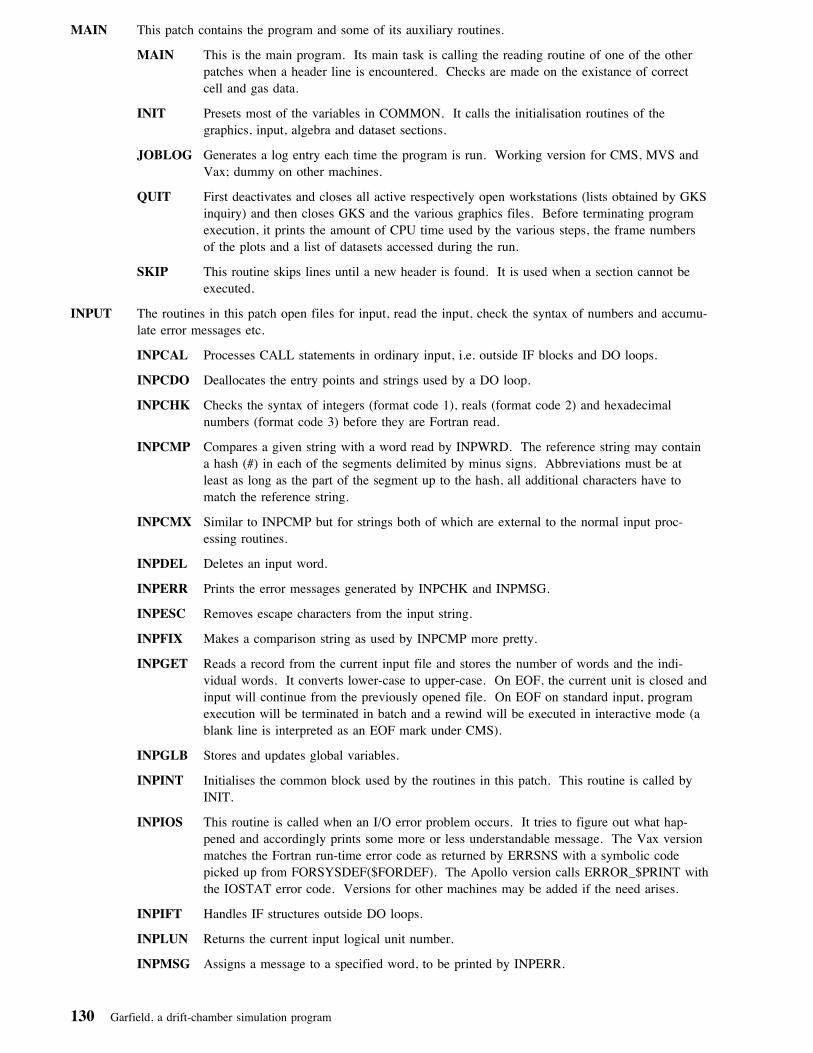
MAIN This patch contains the program and some of its auxiliary routines.

MAIN This is the main program. Its main task is calling the reading routine of one of the otherpatches when a header line is encountered. Checks are made on the existance of correctcell and gas data.

INIT Presets most of the variables in COMMON. It calls the initialisation routines of thegraphics, input, algebra and dataset sections.

JOBLOG Generates a log entry each time the program is run. Working version for CMS, MVS andVax; dummy on other machines.

QUIT First deactivates and closes all active respectively open workstations (lists obtained by GKSinquiry) and then closes GKS and the various graphics files. Before terminating programexecution, it prints the amount of CPU time used by the various steps, the frame numbersof the plots and a list of datasets accessed during the run.

SKIP This routine skips lines until a new header is found. It is used when a section cannot beexecuted.

INPUT The routines in this patch open files for input, read the input, check the syntax of numbers and accumu-late error messages etc.

INPCAL Processes CALL statements in ordinary input, i.e. outside IF blocks and DO loops.

INPCDO Deallocates the entry points and strings used by a DO loop.

INPCHK Checks the syntax of integers (format code 1), reals (format code 2) and hexadecimalnumbers (format code 3) before they are Fortran read.

INPCMP Compares a given string with a word read by INPWRD. The reference string may containa hash (#) in each of the segments delimited by minus signs. Abbreviations must be atleast as long as the part of the segment up to the hash, all additional characters have tomatch the reference string.

INPCMX Similar to INPCMP but for strings both of which are external to the normal input proc-essing routines.

INPDEL Deletes an input word.

INPERR Prints the error messages generated by INPCHK and INPMSG.

INPESC Removes escape characters from the input string.

INPFIX Makes a comparison string as used by INPCMP more pretty.

INPGET Reads a record from the current input file and stores the number of words and the indi-vidual words. It converts lower-case to upper-case. On EOF, the current unit is closed andinput will continue from the previously opened file. On EOF on standard input, programexecution will be terminated in batch and a rewind will be executed in interactive mode (ablank line is interpreted as an EOF mark under CMS).

INPGLB Stores and updates global variables.

INPINT Initialises the common block used by the routines in this patch. This routine is called byINIT.

INPIOS This routine is called when an I/O error problem occurs. It tries to figure out what hap-pened and accordingly prints some more or less understandable message. The Vax versionmatches the Fortran run-time error code as returned by ERRSNS with a symbolic codepicked up from FORSYSDEF($FORDEF). The Apollo version calls ERROR_$PRINT withthe IOSTAT error code. Versions for other machines may be added if the need arises.

INPIFT Handles IF structures outside DO loops.

INPLUN Returns the current input logical unit number.

INPMSG Assigns a message to a specified word, to be printed by INPERR.


INPNUM Returns the number of words the last read string contains.

INPPRM Modifies the prompt string.

INPRAW Returns the entire input string as read from the input stream.

INPRDH Reads an hexadecimal number from a specified word, returns an integer.

INPRDI Reads an integer from a specified word, which should have been checked previously byINPCHK.

INPRDO Reads a DO loop, stores all lines in it, translates all algebra.

INPRDR Reads a real number from a specified word, which should have been checked previously byINPCHK.

INPRIC Checks a integer on syntax, reads it and returns it to the calling routine. This routine doesnot use the information from INPWRD.

INPRRC Checks a real on syntax, reads it and returns it to the calling routine. This routine does notuse the information from INPWRD.

INPSTR Returns part of the string last read.

INPSUB Substitutes global variables in a string about to be passed back.

INPTRA Does input translation. The routine has entries INPTRI for initialisation, INPTRD fordisplay of the table, INPTRG for table retrieval, INPTRR reading the translation commandsand INPTRW for writing the table to a dataset.

INPTYP Does a crude type determination for a given input word.

INPWRD Calls INPGET to read a line and checks the line on use of special symbols as follows:

• first character '<': a new input file is opened,

• first character '>': output is redirected,

• first character '$': command is passed to the environment,

• first character '*': line is ignored,

• first character '%': the line is passed to DSNINP,

• first character '!': the line is passed to GRAINP,

• first character '?': the line is passed to HLPINP.

In all these cases, a new line will be read by INPGET. This routine also takes care ofcalling sub-sections, having DO-loops, IF-lines and IF-blocks processed, definition of globalvariables etc. The net result is that the sections calling this routine do not see input notmeant for them.

INPXDO Executes a DO loop, including any IF statement embedded in it.

HELP A patch providing on-line help.

HLPCNT (Not on Vax.) This routine calculates the number of records the packed help file willcontain.

HLPDEB Prints the entire help file, used for debugging.

HLPINP The Vax version of this routine calls LBR$OUTPUT_HELP. The versions for othermachines read a packed help file called HELP$GARFIELD, GARFIELD PACKHELP orsimilar which is prepared by HLPPAC.

HLPINQ Determines whether some topic exists on the help file or not.

HLPPAC Reads the raw help file HELP_RAW$GARFIELD, GARFIELD RAWHELP or similar,which is in the Vax .HLP input format, and transforms it into a direct access file (packedfile) called HELP$GARFIELD, GARFIELD PACKHELP or similar. The direct access fileconsists of blocks of text each preceded by a link record that contains the record numbers


of the link records of all its subtopics, in addition to its own topic string and the number ofrecords of the topic itself. The root record is located at record 1.

HLPPRT Prints a topic.

HLPSUB Prints the list of subtopics associated with a given topic.

DATASET Some routines manipulating datasets for input and output.

DSNCMP Compares the member creation date with the date of the latest format modification. Usedto ensure that cell and gas datasets can be read successfully.

DSNFMT The Vax version of this routine resolves wildcard characters in the file specification, if any,and substitutes user supplied defaults for file name components, calling LIB$FIND_FILE.The routine has an entry DSNFMD for setting the default file name.

DSNINP Interprets dataset instructions (lines starting on %). If the first command is only a % sign,the routine will loop until it finds EXIT, no further % signs being needed.

DSNLOC Scans through the dataset currently open on unit 12, looking for the member name specifiedin its calling sequence.

DSNLOG Writes an entry in a log for dataset usage (cells, gas, SCEPTRE). The routine has an entryDSNPRT to print out the log records.

DSNOPN The VM/CMS version of this routine works via an exec written to disk and executed viaDSNVMX. The exec replaces = signs in the file specification by the correspondingdefaults then lists all files matching the specification and then eliminates files that haveimproper format and files that can not be written to if such access is requested. If outputhas to be written to a library, the file is either requested to exist on a disk to which the userhas write access or not to exist, explicitly specified and to be located on a disk to which theuser has write access. A file is only opened for reading if the file exists. If more than onefile satisfies all requirements, the first file as listed by LISTFILE will be accessed. If thedisk on which the file is (to be) located has been modified since the last ACCESS, the diskis ACCESSed again. No access if granted to a file that is currently accessed by anotheruser, if the program can determine such access is indeed taking place. This routine has anentry DSNFMD for setting a default file.

The version of this routine for other machines carries out similar checks but from Fortran.Wildcards are only allowed on Vax computers, where they are resolved by DSNFMT.

DSNVMX Writes a REXX exec to disk, executes it and returns the return code to the calling routine.

ALGEBRA The routines in this patch handle formulae. More detailed descriptions of some of them are in Section4.5 on page 116.

ALGCAL Takes care of procedure calls from instruction lists.

ALGCLR Marks an entry point for deletion. The instruction sublist and the memory associated withit can later on be freed by ALGGBC.

ALGEDT Is a very modest editor for instruction lists, mainly used for debugging ALGPRE andALGEXE.

ALGERR Prints the number of arithmetic errors counted by ALGEXE/ALGEX2 since the last call toALGERR.

ALGEXE Executes a set of instructions from the selected sub-list. The routine checks to some extentwhether the entry point information for the requested sub-list is consistent with the inputparameters.

ALGEX2 Performs the calculations on numbers for ALGEXE, only one instruction is processed at atime. This routine is also called from ALGPRE to evaluate constant subexpressions.

ALGEX3 Performs the calculations on logicals for ALGEXE, only one instruction is processed at atime. This routine is also called from ALGPRE to evaluate constant subexpressions.


ALGEX4 Performs the calculations on strings for ALGEXE, only one instruction is processed at atime. This routine is also called from ALGPRE to evaluate constant subexpressions.

ALGGBC Garbage collect of the algebra storage: instruction list, registers and entry point table.

ALGINT Initialisation routine called from INIT.

ALGPRE The heart of this section, converts a formula to a set of instructions. It has an entryALGSIM to simplify an instruction list.

ALGPRT Prints (part of) the instruction list in a, hopefully, more or less readable format.

GRAPHICS The plotting calls in the program are those suitable for a GKS compilation. The routines in this patchtake also care of the graphics initialisation.

GERHND Catches the error messages produced by GKS. It writes its output to logical unit 10, likeGKS itself, rather than to standard output. For a few frequently occurring errors, anexplanatory note is added.

GPL2 Similar to GPL, but for double precision arguments.

GRACWK Activates a workstation.

GRADWK Defines a workstation.

GRCLWK Closes a workstation.

GRDAWK Deactivates a workstation.

GRDLWK Deletes a workstation.

GRDLWK Opens a workstation.

GRAINP This routine reads the graphics (subsection) commands.

GRALOG Keeps a list of plots being made. This routine has an entry GRAPRT to print out the list.

GRALPH Switches the terminal to alphanumeric mode.

GRAPOL Draws a polar coordinate system, see also GRCART.

GRATTR Reads the representations of the various primitives.

GRATTS (Entry in GRATTR) Changes the attributes of GKS primitives according to the item to beplotted.

GRATTG (Entry in GRATTR) Reads a representation table.

GRATTW (Entry in GRATTR) Writes a representation table.

GRAXIS Calls either GRCART or GRAPOL, with labels for the axis.

GRCART Draws a neat set of Cartesian axis.

GRCBIS Is an auxiliary routine of GRCONT; searches via bisection for the point at which thecontour crosses a grid segment.

GRCGRA Is an auxiliary routine of GRCTRA; returns the function gradient.

GRCLAB Is an auxiliary routine of GRCPLT; plots a piece of the contour, adding labels with func-tion values if requested.

GRCMIN Is an auxiliary routine of GRCUPD; minimises the distance between a grid point and acontour segment.

GRCOLC Returns a flag indicating whether a given workstation has colours. Value 1 means nocolours, 0 means colours, -1 means the output is going to WISS or MO for which there isno way to determine whether the final output device has colours or not.

GRCOLR Reads instructions defining new colours, also serves for inquiries.


GRCOLD (Entry in GRCOLR) Returns a short descriptive string used by GRATTQ. It returns eitherin RAW format or in FORMATTED format, in the latter INPFIX is called to remove thehashes and to change to lower case.

GRCOLQ (Entry in GRCOLR) Displays information about colours in full detail.

GRCOLG (Entry in GRCOLR) Reads a list of colours from dataset.

GRCOLW (Entry in GRCOLR) Writes a list of colours to dataset.

GRCOMM Plots a small comment line, like the cell id.

GRCONT Plots contours.

GRCPLT Buffers contour points and calls GRCLAB to plot when the buffer is full.

GRCTRA Auxiliary routine of GRCONT; follows a contour from the starting point found byGRCBIS. It sends the points to GRCPLT for plotting.

GRCUPD Auxiliary routine of GRCUPD; performs the grid updates while the contour is being traced.

GRGRAF Inquires whether the screen may be erased and used for graphics. When running withGTS-GRAL/GKS, the screen is switched to graphics mode as soon as the return key is hit.

GRGRPH Plots a graph, given a set of data-points.

GRGRP2 The same as GRGRPH but for double precision arguments.

GRHIST Plots a histogram.

GRINIT Initialises the graphics and opens graphics output and error logging files.

GRLINE Calls GPL after taking a base-10 log of the coordinates to be plotted on a logarithmic scale.

GRMARK Calls GPM after taking a base-10 log of the coordinates to be plotted on a logarithmicscale.

GRMENU Shows a menu of options for interactive graphics. Two versions exist: one for GTS-GRALup to version 2.6 and one for other flavours of GKS and later versions of GTS-GRAL.

GRMETA Decodes the command line options concerning the metafile.

GRNEXT Clears the screen, it issues a clear workstation or TVNEXT command.

GRAOPT Decodes some options such as logarithmic/linear scales.

GRTERM Decodes the command line options concerning the terminal.

GRTEXT Plots text at a give position. It differs from the GKS routine GTX in that the text is alwaysplotted in NT=0, so as to avoid distortion.

GRQIWK Returns the workstation identifier when given the name.

ROUTINES Most general purpose routines are contained in this patch.

BOOK Allows several facilities to be booked, released etc so that they are not used in parallel byseveral routines.

BTEXT A routine sending the name of the step currently executed to the B-display of a CDC com-puter. It uses the COMPASS routine BDISP (contained in the same deck). This routinehas been tested on the NIKHEF CYBER 173, which perished some time ago, only.

CFMCTR Transforms from Cartesian to internal coordinates.

CFMCTP Transforms polar to Cartesian coordinates.

CFMRTC Transforms from internal to Cartesian coordinates.

CFMRTP Transforms internal to polar coordinates.

CFMPTC Transforms polar to Cartesian coordinates.

CFMPTR Transforms polar to internal coordinates.


CF2RTC CFMRTC for double precision arguments.

CF2RTP CFMRTP for double precision arguments.

CLIP Clips a line segments to the size of a given box, for real arguments. It returns IFAIL=1 ifthe line segment has length 0 after clipping but it does not print an error message if thishappens.

CLIP2 Identical to CLIP but for double precision arguments.

CROSS Determines whether two straight lines cross at an intermediate point for both lines.

DATIMH (Vax only) Returns the current date and time, both as character*8. On all other machinesthe CERN library routine DATIMH (Z007) is used.

F010 (NAG-numerical-routines compilation only.) Is a set of matrix routines replacing part ofthe CERN library F010 package. DEQINV inverts and solves a set of double precisionequations, calling F01ACF and F01AAF. DEQN merely solves the set of equations, notsetting a proper inverse. Its replacement uses F03AFF and F04AHF. REQN is similar toDEQN, the main difference being that the default accuracy parameter X02AAF is not usedbecause the data are single precision.

CRNERR Interface to the KERNLIB error handling routines (N001).

INTERP Interpolates using the spline coefficients calculated by SPLINE. An IFAIL=1 error condi-tion is set if the value for which the interpolation is to be carried out, is out of range.

INTER2 Identical to INTERP but for double precision arguments.

INVINT Finds the point at which the cumulative distribution of the input distribution reaches somethreshold.

LSQFIT Performs a least squares fit of a one dimensional set of data to a general function.

NORRAN (NAG-numerical-routines compilation only.) Returns a normally distributed randomnumber. It uses the NAG routine G05DDF and replaces the CERN library routine V101.

OUTFMT Formats numbers into text.

RNDEXP Generates random numbers according to a exponential distribution.

RNDM (NAG-numerical-routines compilation only.) Returns a uniformly distributed randomnumber. It uses the NAG routine G05CAF and replaces the CERN library routine V104.

RNDNOR Generates normally distributed random numbers with a given mean and standard deviation.It uses the library routine NORRAN.

ROUND Rounds a range to some decent values, such that the interval is reasonable too.

SPLINE Prepares a cubic spline interpolation for a list of REALs. If the x-array is not in strictlyincreasing order an IFAIL=1 error condition is returned, the coefficients are not correct inthis case.

SPLIN2 Identical to SPLINE but for double precision arguments.

STRBUF A dynamic string buffer.

TIMLOG Stores the string it is called with together with the amount of CPU time used since theprevious call. It prints its data when called with an empty string. Use is made of thelibrary routine TIMED. The VM/CMS vector compilation also calls assembler routineswritten by Michel Roethlisberger/IBM to obtain the fraction of time spent in the vectorunits.

VMCMS A skeleton to make a routine that passes commands to VM/CMS.

WLDCRD Determines whether a string matches a wildcard.

HISTOGRAM A set of routines for histogram handling.

HISADM Book-keeping of histograms.


HISENT Enters numbers into a histogram, performing automatic scaling if requested.

HISGET Reads a histogram from a dataset.

HISINT Initialisation of the histogram routines, called from INIT.

HISPRT Prints a histogram.

HISPLT Plots a histogram using GRHIST.

HISSCL Scales a histogram by a given factor.

HISWRT Writes a histogram to a dataset.

VAXAST A set of routines written by Carlo Mekenkamp (University of Leiden, Netherlands) handling control-Cinterrupts on a Vax.

See writeup Z037 of the CERN program library for information.

CELL This patch contains the routines defining the cell.

CELDEF Is called by TEST and its main task is to call the other routines in this patch. It returns toTEST as soon as one of them fails.

CELINP This routine reads all the cell description input and stores them in common CELDAT.

CELCHK Tries to make sure that the cell makes sense (it eliminates wires outside planes or wires tooclose to each other). The routine sets the default cell dimensions and stores the maximumand minimum voltages in the cell.

CELTYP Determines the potential to be used for the field calculations. It sets quasi-periodicities forthe B and C type cells.

CELPRT Prints all available cell data.

CELPLT Prepares a frame in which a layout of the cell will be plotted.

CELLAY This routine does the actual plotting of the layout. It is called from many other routines aswell.

CELWRT In a first stage this routine isolates a dataset name from its input string and stores it. In asecond stage all available cell data are written.

CELGET Reads cell data from a dataset written by CELWRT.

WIRSEL Selects wires for special treatment.

MAGINP Reads magnetic field data and calculates the α coefficient (see Section 4.1.11 onpage 105). It computes the cylindrical components of the magnetic field.

GAS The routines in this patch do the same job as the cell routines i.e. they read gas data, store it in asuitable format and provide the requested information to other sections.

GASDEF Calls the other routines in this patch during a gas section. It checks the IFAIL flag aftereach call and returns to the main program as soon as an error is found. GASDEF has anentry XXXGAS that loads CO2 in case gas data is needed but no gas has been entered.

GASINP Reads gas data from input file. This routine can, instead or reading data, call one of theroutines filling the gas data common block directly.

GASCHK Checks the correctness of the gas data entered in GASINP and sets the GASOK bitsaccordingly.

GASMIX Computes the drift velocity and diffusion in a mixture of gasses.

FGAS1 Used to integrate F0.

FGAS2D Used to calculate the diffusion.

FGAS2N Used to normalise F0.

FGAS2V Used to calculate the drift velocity.


GASMXB Returns information on the gas data, such as a list of break points, the name, the ionisationpotential.

GASMXD Returns the cross section, mean free path and average energy loss per collision.

GASMG1 Used to calculate integrals.

GASMG2 Used to calculate integrals.

GASPRE Prepares the interpolation of the drift-velocity, the diffusion and the Townsend coefficient.It also sets the coefficients for the extrapolations.

A20E80 Transfers a mixture of 20 % argon and 80 % ethane to /GASDAT/.



A73M20 Transfers a mixture of 73 % argon, 20 % methane and 7 % propanol to /GASDAT/.

CO2 Transfers the CO2 data to the /GASDAT/ common block.

C80E20 Transfers a mixture of 80 % CO2 and 20 % ethane to /GASDAT/.

C90E10 Transfers a mixture of 90 % CO2 and 10 % ethane to /GASDAT/.

C90I10 Transfers a mixture of 90 % CO2 and 10 % isobutane to /GASDAT/.

ETHANE Transfers the ethane data to the /GASDAT/ common block.

ISOBUT Transfers the isobutane data to the /GASDAT/ common block.

METHAN Transfers the methane data to the /GASDAT/ common block.

GASPRT Prints tables of the diffusion and drift-velocity and lists the other relevant gas quantities(such as A, Z, ρ etc.).

GASPLT Makes logarithmic plots of the diffusion coefficient and of the drift-velocity and ahistogram of the cluster-size distribution.

GASWRT In a first stage a dataset name is extracted from command line. In the second stage all gasdata (including the spline coefficients and the cluster-size histogram) are written to thisdataset.

GASGET Retrieves the gas data written by GASWRT.

DRIFTV Returns the magnitude of the drift-velocity for electrons given the electric field-strength. Itinterpolates the tables.

DIFFC Similar to DRIFTV but for the diffusion coefficient.

GASTWN Returns the Townsend coefficient for a given field-strength.

OPTIMISE

OPTADD Adds elements to the cell.

OPTCHV Changes the potential of a selected group of wires and then recalculates the charges.

OPTDEL Deletes elements from the cell.

OPTFAC Splits the field and the potential into pieces proportional to the wire potentials and a con-stant part.

OPTINP Reads optimisation instructions and calls the other routines in this patch when needed.

OPTSET Attempts to make a given field-function as equal to a given target-function as possible byplaying with the potentials.

OPTFUN Used by OPTSET in the minimising cycles.

OPTXYA Selects the points at which the field-function and the target-function are to be evaluated. Italso sets the initial values of the parameters.


OPTAVE Computes the average of the field-function.

OPTDSN Saves and restores sets of potentials.

FIELDPLOT A patch consisting of set of routines producing the plots and tables of the potential, the electric fieldand the magnetic field.

FLDINP Reads the plot parameters from standard input and calls the other routines in this patchwhen some action is required.

FLDPLT Makes the plots specified in the command line.

FCONT A subroutine called by the NAG graphical supplement library routines returning a fieldfunction to be used by the contour plotting subroutine.

FLDPRT Prints the field quantities listed in the input string.

FLDCHK This routine is useful for the debugging of the field routines as it allows checking of thepotentials on the wires and the planes, of the consistency between the potential and theelectric field, of the charge on the wires and of the Maxwell relations ∇E = 0 (outside thewires) and ∇B = 0 (if there is a magnetic field).

ZERO Routines locating the zeros of the field.

ZROARG Returns the argument of the field at some point on the boundary of the current search area.

ZROCNT Counts the number of zeros in the current search area, using the change in argument.

ZROFND Controls the other routines. It builds a stack of search areas which are divided into two ateach iteration.

ZROLOC Attempts a precise localisation of the zero within the current search area.

ZROTST Debugging routine for zero finding.

FIELDCAL Responsible for electric fields and potentials and magnetic fields.

SETUP Calls one of the more specific SET... routines:

SETNEW Calculates the charges for a new set of voltages, without recalculating the capacitancematrix.

SETA00 for non-periodic cells,

EFQA00 for non-periodic cells with dielectrica,

SETB1X for x-periodic cells and at most one plane at constant x,

SETB1Y for y-periodic cells and at most one plane at constant y,

SETB2X for cells with (the equivalent of) 2 planes at constant x,

SETB2Y for cells with (the equivalent of) 2 planes at constant y,

SETC10 for cells periodic in x and in y without planes,

SETC2X for y periodic cells with (the equivalent of) 2 planes at constant x,

SETC2Y for x-periodic cells with (the equivalent of) 2 planes at constant y,

SETC30 for cells with (the equivalent of) 2 planes at constant x and 2 planes at constant y.

'the equivalent of' is to be interpreted as having 2 planes or having one plane and being periodic in thesense orthogonal to the plane. These routines fill a capacitance matrix stored in common /CAPAC/later to be accessed by:

CHARGE Inverts the capacitance matrix and determines the charges on the wires. If no equipotentialplanes are present, the net charge on the wires will be 0. This may imply that the referencevoltage is different from 0.

When all this has been done the electric field may be calculated:


EFIELD Checks that the point at which the electric field is to be evaluated is not located inside awire or outside a plane (after reduction to the elementary cell) and calls one of the fieldroutines EFC...:

EFCA00 (scalar and IBM vectorisable version available) for non-periodic cells,

EFDA00 for non-periodic cells with dielectrica,

EFCB1X (scalar and IBM vectorisable version available) for x-periodic cells and at most one plane atconstant x,

EFCB1Y (scalar and IBM vectorisable version available) for y-periodic cells and at most one plane atconstant y,

EFCB2X (this routine is IBM vectorisable) for cells with (the equivalent of) 2 planes at constant x,

EFCB2Y (this routine is IBM vectorisable) for cells with (the equivalent of) 2 planes at constant y,

EFCC10 (only available in scalar form) for x- and y-periodic cells without planes,

EFCC2X (only available in scalar form) for y periodic cells with (the equivalent of) 2 planes at con-stant x,

EFCC2Y (only available in scalar form) for x periodic cells with (the equivalent of) 2 planes at con-stant y,

EFCC30 (only available in scalar form) for cells with (the equivalent of) 2 planes at constant x and 2planes at constant y.

PH2 (Written by G.A. Erskine, somewhat modified.) Computes essentially the logarithm of theϑ1 function. This routine is used only for the potential calculations in C type cells. It hasan entry PH2LIM for the diagonal terms.

E2SUM (Written by GA Erskine, substantially modified.) Computes the logarithmic contribution tothe electrostatic field. This routine is used only for the field calculations in C1 type cells.

Some routines needed later on for dielectrics and multipole terms are already to be found in this patch:

EFCMAT Computes correction factors for the field.

EFMWIR Decomposes the field around a wire in a multipole series.

EFDFUN Function used by EFDWIR, returns a sum of Legendre polynomials.

Magnetic fields are calculated by:

BFIELD Its only task is calling one of the 4 following routines:

MAG00 magnetic field calculation for non-periodic cells,

MAGX0 magnetic field calculation for x-periodic cells,

MAG0Y magnetic field calculation for y-periodic cells,

MAGXY magnetic field calculation for x- and y-periodic cells.

DRIFT The routines in this patch plot drift-and equal arrival time lines.

DRFARR Calculates arrival time distributions.

DRFDRF Calls DRFEDG, DRFTRA, DRFWIR or DRFZRO when drift line plots have to be made.

DRFEDG Does the same as DRFWIR but now the drift-lines start at the edges of the drift-area.

DRFEQT The routine DRFEQT accumulates equal time data on the current drift-line. Doing so, itcounts the number of errors and memory overflow. The entry DRFEQP outputs the datastored so far, plotting separate sets of contours for each wire, checking that equal timecontours do not cross drift-lines. The second entry DRFEQR resets the number of contoursto 0. The third entry DRFEQE prints the number of errors found by DRFEQT.

DRFGRA Executes drift section commands selected via a graphics menu.


DRFINP Reads instructions from input file and calls one of the other routines when some action isrequired.

DRFPLT This routine examines the DRIFT instruction and calls either DRFEDG or DRFTRA,DRFWIR or DRFZRO as appropriate providing them with arguments.

DRFSIN Plots and prints information on individual drift lines.

DRFTRA Does the same as DRFWIR but now the drift-lines start on a track.

DRFTR2 Plots the graphs for which DRFTRA has accumulated the data.

DRFTAB Makes a drift-time table, printing the output or plotting it in the form of a rough contourdiagram (using NAG routines).

DRFWIR This routines has DLCALC calculate drift-lines starting near the surface of the sense wiresand plots them. It calls DRFEQT to store points on equal arrival time contours.

DRFXTP Produces a so-called x(t)-plot, see Section 4.3.3 on page 112. It has two auxiliary routines:

DRFXT1 Calculates the point at which the current drift-line crosses a straight line with given parame-ters. It uses a simple linear interpolation, which was found to be more accurate than a thirdorder fitting.

DRFXT2 Returns the minimum of a parabola passing through three given points. It gives an indi-cation whether the parabola is degenerate and whether the 'minimum' is in reality amaximum.

DRFZRO Plots drift-lines from the zeros of the field.

DRIFTCALC This is the core of all routines needing drift-lines.

DLCALC This very important routine calculates a drift-line and stores it in the common /DRIFTL/.How the drift-line is calculated is described in detail in Section 4.3 on page 110 of thiswriteup. After each integration step DLCSTA is called and the status code returned by thisroutine is examined and appropriate action is taken. During each step, both DLCALC andDLCSTA can call the auxiliary routines DLCWIR, DLCPLA and DLCMIN.

DLCSTA This routine checks the status of the drift-line after each integration step. Each step, aprobable target wire is selected which DLCALC will use during the next step to seewhether a wire has been crossed. The ISTAT code has the following meaning: 0: calcu-lation in progress, -1: left drift-area, -2: maximum number of steps (MXLIST) reached, -3:abnormal end or particle stopped, -4: particle hit a plane, 0 < ISTAT ≤ MXWIRE: particlehit wire ISTAT, ISTAT > MXWIRE: particle hit a periodic replica of wireISTAT-MXWIRE. A non-zero code normally means that some last step has to be per-formed by this routine (or DLCWIR or DLCPLA) and that DLCALC will stop. The rou-tines called by instructions mentioned in Chapter 2.0 on page 3 will interpret the statuscodes but the debugging routines/options usually print the raw results.

DLCWIR Terminates the drift-line by stepping towards the target wire by means of the dedicated wirealgorithm described in the paragraph on drift-line integration (see Section 4.3.2 onpage 111).

DLCMIN Determines the minimum distance between the target wire during the step.

DLCPLA Terminates the drift-line by stepping towards a plane.

DLCPRO Projects 3-dimensional drift lines onto a specified 2-dimensional plane.

DLCVEL Calls EFIELD to find the electric field-strength at a given position and then calls DRIFTVto find the drift-velocity for this field-strength. The magnetic field routines are also calledin case a magnetic field has to be taken into account. High B field corrections, such asthose described in [1] may have to be introduced in this routine.

DLCDIF A service routine which returns a fairly accurate estimate of the integrated diffusion coeffi-cient over the present drift-line.


DLCTWN A service routine which returns a fairly accurate estimate of the integrated electron multipli-cation factor over the present drift-line.

DLCTRP Calculates drift-lines from a track, storing the data in a format suitable for interpolation.

DLCTRI Interpolates the track-data prepared by DLCTRP.

DLCTRW Writes the data prepared by DLCTRP to a file.

DLCTRG Retrieves the interpolation-data from a file written by DLCTRW.

SIGNAL The signal simulation patch

SIGINP This routine controls the other routines in this patch. It interprets the instructions and assoon as simulation is requested, the routine SIGGEN will be called. It tells SIGGENwhether the signal matrices and the ion-tails may be reused or not.

SIGGEN Controls the signal simulation.

SIGIPR Stores the signal matrices, Fourier transforms them, inverts them and transforms them backto the original domain.

IPRA00 Signal matrix calculation for cells with reduced cell type A.

IPRB2X Signal matrix calculation for cells with reduced cell type B2X.

IPRB2Y Signal matrix calculation for cells with reduced cell type B2Y.

IPRC30 Signal matrix calculation for cells with reduced cell type C3.

IONBGN Opens the scratch file used for signal matrices and determines the most efficient format,given the maximum record length allowed by the disks MXRECL and the maximumnumber of records (1000).

IONIO Performs the actual I/O operations for SIGIPR. It shares a common block with IONBGNtelling it how to read/write the matrices. The routine reads/writes only those sections ofeach matrix that will be/have been modified by SIGIPR.

SIGCLS Generates positions and energies for clusters along the track. It also calculates the arrivaltimes for each of the primary electron ion pairs and their charge after avalanche.

SIGAVA Does the avalanche calculation for SIGCLS.

EPULSE Adds a spike to the signal.

SIGION Adds an ion-tail to the signal, it keeps the signals it has calculated unless changes occur. Itneeds (amongst others) SIGFLD.

SIGFLD Calculates the electric field in the non-periodic cell via one of the more specific routines:

IONA00 for cells with reduced periodicity A,

IONB2X for cells with reduced periodicity B2X,

IONB2Y for cells with reduced periodicity B2Y,

IONC30 for cells with reduced periodicity C3.

SIGPLT Plots the pure and cross-induced signals obtained.

SIGWRT Outputs the signals to a file of which the name was established in a first call from SIGINP.

SIGCHK Runs a couple of checks on signal related calculations.

SIGTHR Computes arrival time distributions. The routine has a series of auxiliary routines.

6.4 Program history1/9/84 (At CERN) First version, written in Siemens Fortran 77, ready for use with MVS. It contained the basic

features of the present program but was far less elaborate.


1/2/85 (At NIKHEF-H) A program which could be run on Apollo and CDC too, was sent to CERN. By then, thelanguage had become standard Fortran 77. Use in an interactive environment has been supported fromthen on. The field calculations in C cells was improved.

15/5/85 (At CERN) An entirely new, much expanded signal section was introduced. The drift-line calculation rou-tines were replaced by more stable ones. New were magnetic field, sense wire selection and theCHECK instruction.

15/2/86 (At CERN, Leiden) Because of the introduction of VM/CMS at CERN, the GD3 plotting calls werereplaced by their GKS equivalents, adding interface routines for both miniGD3 and GD3. The ratherstrange "features" of VM/CMS called for many changes in file handling. In this version free formatinput, algebraic formula handling, cylindrical symmetry, 3 new standard gasses and the APOLLOcommand were added. Field calculation was speeded up by 10 to 40 %.

7/7/86 (At CERN, Leiden) The x(t) routine was replaced by a much more accurate one. The formula used so farfor calculating the drift-velocity if magnetic fields are present turned out to be inadequate and washence replaced. File handling and cylindrical symmetry routines were improved. New was theFACTOR instruction.

26/6/87 (In Padova) Numerous corrections are applied in the cylindrical symmetry parts. An instruction to create adrift-time table has been introduced in the drift section. The program can now also be compiled on aVax. The use of the NAG graphics supplement routines has been extended, they can now be used forfield contour plotting, plotting of contours in a drift-time table and for surface plotting.

1/12/87 (at CERN) Major revision of the program because the original construction of the program could no longerbe maintained given its growth. Many routines have been renamed as a consequence. Most modifica-tions should however be transparent to the users. Additions include: dataset access and inquiry, calcu-lation of arrival time distributions, checks on the signal calculation, Townsend coefficients. Replacedare: the x(t) routines, equal time contour routines, the field calculation in C type cells and the drift-linetermination routines. Several hooks for future options have been put into the program. The abbrevi-ation convention has been changed. This writeup has been converted from Cernpaper to SGML (mixedwith Script commands).

1/5/88 (at CERN) Several parts of the program have been refined but no major changes have occurred. The rou-tines for finding and interpreting the zeros of the field, which have been present since about a year,have been made operational. The same applies to the optimisation section. Various graphics settingsare under user control from this version onwards.

1/1/89 (at CERN) The use of Vax features has been extended: on-line help is provided, a template file linked withthe help file has been written and the program is started via CDU. The latter feature allows the specifi-cation of the terminal type at start-up time. The control-C interrupt, present already for a long time,has been further improved by Carlo Mekenkamp. A help facility similar to that on Vax and using thesame input files is available for use on other machines. The program runs successfully on the Cray.Various features such as drift-line calculation under graphics input control have been added.

15/6/89 (at CERN) Dielectrica are being introduced on a test basis. The compilation options GD3, miniGD3 andCDC have been removed. At the same time the use of GKS features has been increased, allowing forinstance user control on the appearance of every part of a plot.

1/9/89 (at CERN) On the occasion of its 5th anniversary, Garfield is introduced in the CERN Program Library.Vectorisable versions for some CPU intensive routines are provided.

1/5/90 (at CERN) The use of NAG contour routines is being reduced because of insufficient availability and theirrather poor quality. The field contours are now being plotted by the programs own routines; drift-timetable contours will follow. An instruction to do calibrations with cluster counting (ARRIVAL) hasbeen added. The program now also runs on Sun computers. Loops and conditionally executed piecesof input have been added.

1/10/92 (AT CERN) Gas mixing routines have been introduced. Global variables now have a type associated withthem, random number generators have been made available.


7.0 Acknowledgments

Garfield has greatly benefitted from the help of many people. In particular the following persons should be men-tioned. Diego Bettoni, for a long time the primary user of the program, carried out a great deal of testing. KarlDederichs provided the CO2 gas data and gave a lot of practical advice. G. A. Erskine did virtually all the work ondoubly periodic potentials and gave valuable advice with respect to the signal calculations. Chris Fabjan, my super-visor during my stay at CERN as a summer-student in '84, introduced me to drift-chambers. Matthias GrossePerdekamp has provided descriptions of argon-ethane and argon-methane gas mixtures. He also compared calcu-lated and measured signals. Ingo Herbst has pointed out how the magnetic field description could be improved andprovided the descriptions of methane and ethane. Discussions with Iouri Ivaniouchenkov were very valuable whenwriting the arrival time distribution routines. Carlo Mekenkamp gave highly useful programming advice, wrotesome of the input and all of the AST routines for control-C interception on the Vax. François Piuz teached memost of what I now know about energy loss in gasses. Alan Rudge explained some of the electronics used in theread-out to me.

Acknowledgments 143


145


Bibliography

[1] A. Breskin et al., Nuclear instruments and methods,124 (1975) 189-214.

[2] G. Schultz and J. Gresser, Nuclear and Instrumentsand Methods, 151 (1978) 413-431.

[3] Fabio Sauli and Anna Peisert, Computer programmeto compute drift velocities and diffusion coefficientsin gas mixtures.

[4] J. Fehlmann,, WIRCHA, a program package to simu-late drift chambers (ETH-Zurich, 1985).

[5] F. R. A. Hopgood, D. A. Duce, and J. R. Gallop,Introduction to the Graphical Kernel System (GKS),Academic Press (1983).

[6] GTS-GRAL, GKSGRAL / GKSGRAL-3D Referencemanual (GTS-GRAL Darmstadt, February 1987).Note: Also as a CERN report: CERN/DD/US/102.

[7] F. Sauli, Principles of operation of multiwire propor-tional and drift-chambers (CERN, 77-09, 1977).Note: Lectures given in the Academic Training Pro-gramme of CERN 1975-1976.

[8] L. D. Landau,, J. Phys. (USSR), 8 (1944) 201-205.Note: in: L. D. Landau, Collected papers, page 417,ed. D ter Haar, Pergamon Press Oxford, 1965..

[9] K. S. Kölbig and B. Schorr, Computer Physics Com-munications, 31 (1984) 97-111.

[10] I. A. Markushevich, Theory of functions of a complexvariable, Vol. II, p. 292, Prentice-Hall (1965).

[11] R. T. Whittaker and G.N. Watson, A course of modernanalysis, Chapter 21, Cambridge (1927).

[12] R. T. Whittaker and G.N. Watson, A course of modernanalysis, Section 21.11, Example 3, Cambridge(1927).

[13] H. Buchholz, Elektrische und magnetischePotentialfelder, section 3.11, Springer (1957).

[14] C. W. Clenshaw, Mathematical Tables & Aids toComputation [Journal name later changed to Math-ematics of Computation], 9 (1955) 118-120.

[15] Jerold E. Marsden, Basic Complex Analysis, Chapter5, W. H. Freeman and Company (1973).

[16] Jerold E. Marsden, Basic Complex Analysis, Section6.2, p. 319-322, W. H. Freeman and Company (1973).

[17] E. Durand, Magnétostatique, Masson, Paris (1968).

[18] Konrad Kleinknecht, Detektoren fürTeilchenstrahlung, Teubner (1984).

[19] J. Stoer, Einführung in die numerische Mathematik,Vol. I, 2nd Ed., Springer HTB (1978).

[20] J. Stoer and R. Bulirsch, Einführung in die numerischeMathematik, Vol. II, 2nd Ed., Springer HTB (1978).

[21] Laurent Schwarz, Méthodes mathematiques pour lessciences physiques, Chapitre IV, deuxième édition,Hermann (1979).

[22] F. Lapique and F. Piuz, Nuclear Instruments andMethods, 175 (1980) 297-318.

[23] G. A. Erskine, Nuclear Instruments and Methods, 198(1982) 325-336.

[24] J. H. Jeans, Electricity and magnetism, 5th Ed.,Cambridge University (1951).

[25] W. R. Smythe, Static and dynamic electricity, 3rd Ed.,McGraw Hill (1968).

[26] Matthias Grosse Perdekamp, Aufbau einesDriftkammersystems für Myon NukleonStreuexperimente., Diplomarbeit, University ofFreiburg im Breisgau, Germany (1990).

Bibliography 147


Index

ϑ1 function (definition) 95

Numerics3-D plots

drift section 59of the field 46

AA potentials (description) 93accuracy

drift-line calculations 111field calculations (C potentials) 101signal calculations 67

ACTIVATE-WORKSTATION (graphics command) 79ADD-ENTRY-POINT (algebra command) 87ADD-WORKSTATION (graphics command) 79Aegis commands (from inside the program) 77algebra

entering the cluster size distribution 31entering the gas tables 36method used to evaluate formulae 116order of precedence of operators 119plotting field data 47, 60printing field data 47routine descriptions 132use in the cell section 21

alternate input files 76AREA

drift section 49field section 43optimisation section 39signal section 66

array dimensionschanging them 125error message if too small 12

ARRIVAL-TIME-DISTRIBUTION (drift section) 51attachment coefficients

entering the data 36avalanche

calculation method 114taking into account 69

AVALANCHE (signal section) 66

BB potentials (description) 93B1x potentials (description) 94B1y potentials (description) 94B2x potentials (description) 94B2y potentials (description) 94boundary conditions (electrostatic) 102bugs (in case you find one ...) 2

CC potentials (introduction) 95C1 potentials (description) 95C2 potentials (description) 97C3 potentials (description) 99capacitance equations 102capacitance matrix 102Cartesian coordinates (specifying) 21cell section

command descriptions 21routine descriptions 136

cell types (table) 92CELL-IDENTIFIER (cell section) 21CHANGE-VOLTAGES (optimisation section) 39character input 16charges (electrostatic wire charges) 91CHECK

field section 43signal section 66

CLEAR-AFTER-PLOT (graphics option) 81CLEAR-BEFORE-PLOT (graphics option) 81CLEAR-ENTRY-POINT

algebra command 87CLOSE-WORKSTATION (graphics command) 79CLUSTER function (gas section) 31cluster position 113CLUSTER tabulated (gas section) 31cluster-size distribution 113CMS commands (from inside the program) 76CO2 (gas section) 28COLOUR (graphics command) 79comment lines 75comments in output 74compilation

machine dependent parts 124COMPONENTS (magnetic field section) 27conformal mapping (cylindrical symmetry) 103continuation lines (...) 16contour plots


convolution equations (signals) 116coordinate systems 21cosine function (formulae) 119COUNT (algebra command) 87cradle (Patchy) 125cross-induced signals (taking into account) 69current value (finding out) 16

DD potentials

how they are calculated 102how to use 24

Index 149

datasetscreating a cell dataset 24creating a gas dataset 36creating a signal dataset 71creating an x(t) dataset 64format description 10introduction 10manipulation 77routine descriptions 132

DCL commands (from inside the program) 77DEACTIVATE-WORKSTATION (graphics command) 80DEBUG (option) 74debugging

-debug command line option (Unix) 3, 74-identification command line option (Unix) 3, 74/DEBUG command qualifier (Vax) 8, 74/IDENTIFICATION command qualifier (Vax) 8, 74DEBUG command line option (VM/CMS) 5, 74drift section 61field section 43, 47general remarks 129IDENTIFICATION command line option (VM/CMS) 5,

74option to print debugging output 74signal section 66user test routine 126, 129

DEFAULT (dataset command) 77default values 16DEFINE (cell section) 21DELETE

algebra command 87dataset command 78

DELETE-WORKSTATION (graphics command) 80dielectrica

limitations 1diffusion

calculation method 114entering the data 36lateral (neglected at present) 2taking into account 69

dipole terms (neglected) 1DISPLAY (optimisation section) 39DISPLAY-ENTRY-POINT

algebra command 88distortion of B field 27DRIFT (drift section) 49, 54drift section

command descriptions 49routine descriptions 139

drift-linescalculation method 110, 111routine descriptions 140

drift-time table (obtaining one) 62drift-velocity (formula) 110DUMP-HELP-FILE (dataset command) 78

Eelectron pulses

calculation method 114

electron pulses (continued)taking into account 69

entier function (formulae) 119EPSILON

drift section 56signal section 67use in the integration 111

equal arrival time contours 55, 62equipotential lines 46error messages

generated by Garfield 12generated by GKS 13generated by KERNLIB 74increase MX... 12overflow 13overview 12underflow (error 208 on IBM) 13

ETHANE (gas section) 28EXEC files (running under VM/CMS) 4EXECUTE (algebra command) 88EXIT

algebra command 88graphics command 80

EXTRAPOLATIONS (gas section) 32

FFACTOR (optimisation section) 39field calculation

method used 91notation 91routine description 138

field sectioncommand descriptions 43routine descriptions 138

formulae (description how they are handled) 116FOURIER (signal section) 67Fourier transforms (signals) 116FUNCTION (algebra command) 88

GGARBAGE-COLLECT (algebra command) 88GARFIELD BATCHID 7gas mixtures

calculation method 105command description 28routine description 136

gas sectioncommand descriptions 28routine descriptions 136

GAS-IDENTIFIER (gas section) 32gasses

built-in 28entering a new gas from input 30

GETcell section 21gas section 32

GET-COLOURS (graphics command) 80


GET-REPRESENTATION (graphics command) 81GET-TRACK (signal section) 67graphics

changing the settings 79in case of trouble 13NAG routines 62routine description 133using the NAG graphical supplement 126

GRAPHICS-INPUT (drift section) 56Green reciprocity equations 115GRID

drift section 56field section 44graphics option 81graphics representation 83optimisation section 39

grids of point charges 95

Hheader of an input section 15header record format (datasets) 10help

file inspection 78file preparation 78obtaining help information 76routine description 131

histogramsdrift section 59of the field 46routine description 135

Householder inversion 40

II/O units 129IDENTIFICATION (option) 74image charges 102INDEX (dataset command) 78induced current (expression for) 115input

abbreviation conventions 16assisted by LSE (Vax only) 8format 15from a file 76routine description 130syntax conventions 16

INPUT (option) 74INQUIRE-DEFERRAL-UPDATE-STATE (graphics

command) 81INQUIRE-LEVEL-GKS (graphics command) 81INQUIRE-OPERATION-STATE (graphics command) 81INQUIRE-WORKSTATIONS (graphics command) 81INSERT (algebra command) 88instructions (what they are) 15integration accuracy

numerical details 111setting 56

INTEGRATION-PARAMETERS (drift section) 57

internal coordinates (cylindrical symmetry) 103INTERPOLATION (gas section) 32interrupting program execution

enabling this feature 125on a Vax: additional files needed 123on a Vax: how to do it 9on a Vax: routine description 136under VM/CMS 7

ION-LINES (signal section) 67ion-tails

calculation method 115taking into account 69

ISOBUTANE (gas section) 28isolated charges 93

KKERNLIB error message printing 74

LLandau approximation 113lateral diffusion (neglect of) 114Layout of the cell (making the plot) 22Layout of the cell (printing a table) 22libraries

format description 10introduction 10

line-electrodes 1linear scale 82LINES (drift section) 57LIST

algebra command 88dataset command 78

logarithm (formulae) 119logarithmic scale 82logical record length (CMS datasets) 10logical units 129loop-variable (ROWS statement) 24LORENTZ (drift section) 57Lorentz angle (deviation from real value) 27

MMAGNETIC (section) 27magnetic field calculation 105magnetic susceptibility 105mail address

conventional 2electronic 2

Maxwell equations (checking they are satisfied) 43MEMORY (algebra command) 88metafile type

specifying on Unix 3specifying on Vax 8specifying on VM 5

METHANE (gas section) 28MINIMISE (drift section) 57mirror charges 102MIX (gas section) 28

Index 151

mixtures of gassescalculation method 105command description 28routine description 136

mobilityentering 35scaling properties 111

Model description 91motion of drifting particles 110multiplication factor 114

NNAG

switch to select the graphics routines 126switch to select the numerical routines 126

notation (electrostatics) 91numeric input 16

OOPEN-WORKSTATION (graphics command) 81optimisation section

command description 39routine description 137

OPTIONSalgebra command 88all sections 74cell section 22drift section 59gas section 33magnetic field section 27optimisation section 40signal section 68

output (rerouting to a file) 76overflow (protection against) 13

PPACK-HELP-FILE (dataset command) 78PARAMETERS (gas section) 35Patchy

cradle 125if Patchy is not available 126list of switches 125YLIST (lists a PAM file) 125

Patchy switchesApollo 125ATCGKS 125CERN 125CMS 125Cray 125DECGKS 125DECS 125GTSGRAL 125IBMRT 125MANYWIRE 126MVS 126NAG 126NAGNUM 126PLOT10GKS 126

Patchy switches (continued)SAVE 126SUN 126SUNGKS 126TEST 126VAX 126

PERIOD (cell section) 22periodicity

how it is handled 92how to enter it 22

periodicity (default 103PLANE

cell section 22checking the potentials at the surface 43how a plane is handled 102how a plane is plotted 83

PLOTdrift section 59field section 46

POINTS (optimisation section) 40polar coordinates

how they are handled 103specifying 21

PREPARE-TRACK (drift section) 60PRESSURE (gas section) 35primary electron-ion pairs 113PRINT

algebra command 89field section 47

program bug (message being printed) 12program versions

selection on a Vax 8selection under VM/CMS 6

PROJECT (drift section) 60PURGE (dataset command) 79

Qquadrupole terms (neglected) 1quotes (keep strings together) 16

Rrandom number generators (formulae) 119record format (CMS datasets) 10RECOVER (dataset command) 78redirecting the output 76reference potential 91REGISTER (algebra command) 89REPEAT (signal section) 68REPRESENT (graphics command) 82RESET

algebra command 89cell section 23gas section 35

RESOLUTION (signal section) 68RESTORE (optimisation section) 40RESULTS (algebra command) 89ROWS (cell section) 23


rows of point charges 93Runge-Kutta-Fehlberg integration 111running the program

Cray job submission from VM/CMS 6on a Vax 8on the Cray 4on Unix 3submitting a Cray job 4under VM/CMS 4

SSAMPLE (field section) 47SAVE (optimisation section) 40SAVE statements 126Sceptre electronics simulation

creating a dataset 71section (what it is) 15SELECT

drift section 61field section 47optimisation section 40signal section 68

separators 16SET (optimisation section) 40SET-DEFERRAL-STATE (graphics command) 86SIGNAL (signal section) 68signal section

calculation method 112command descriptions 66routine descriptions 141

signal simulation 112SIMPLIFY (algebra command) 89sine function (formulae) 119SINGLE (drift section) 61special characters

! (graphics settings) 79? (obtaining help information) 76... (continuation lines) 16{} (global variable substitution) 17{} (in command descriptions) 16@ (entering the algebra editor) 87[] (in command descriptions) 16$ (escape to the environment) 76* (comment line) 75* (default value) 16* (wildcard character) 22, 32, 67, 76% (dataset manipulation) 77% (member header record) 10< (alternate input) 76<< (EOF marker) 76> (alternate output) 76| (in command descriptions) 16

SPEED (drift section) 61Spice electronics simulation

creating a dataset 71status code (drift-lines) 112step-size updating 111stopping program execution 73

storage space (if limited) 124strips 1SUBSET mode (CMS) 77suggestions for improvement 2surface plots


susceptibility 105SUSCEPTIBILITY (magnetic field section) 27

TTABLE

drift section 62gas section 35

TEMPERATURE (gas section) 36terminal type

specifying on a Vax 8specifying on Unix 3specifying on VM 5

TEST (algebra command) 89Theta function (definition) 95thin-wire approximation 1, 95TIME

drift section 62field section 47

TIME-STAMP (graphics option) 82timing

drift-line calculations 62field evaluations 47

Townsend coefficientsentering the data 36taking into account 114use in AVALANCHE 66

trace (following the program flow) 74TRACK

drift section 63field section 48graphics representation 84making particles drift from a track 55optimisation section 42signal section 71

TRAPdrift section 63signal section 71

TUBEcell section 24checking the potentials at the surface 43graphics representation 84potentials for tubes 102

Uunderflow (absence of protection) 13units (physical) 19UTEST 126

VVARIABLES (algebra command) 89

Index 153

vector plotsdrift section 59of the field 46

vectorisationcompilation flag 126using the IBM 3090 VF 6

viewing angles3-dimensional field plots 46drift section 59

Wwarnings: see error messages 12wildcards

cell description retrieval 22gas description retrieval 32help facility 76prepared track retrieval 67Vax file names 11

wire charges 91wire-codes

defining 23use for making x(t)-plots 61use for signal calculations 68use in FIELD section 47

wire-diameter (entering the value) 23workstations

activating 79closing 79deactivating 80defining 79deleting 80inquiry 81opening 81requesting metafile output on a Vax 8requesting metafile output on Unix 3requesting metafile output on VM 5requesting terminal output on a Vax 8requesting terminal output on Unix 3requesting terminal output on VM 5

WRITEcell section 24gas section 36

WRITE-COLOURS (graphics command) 87WRITE-EQUAL-TIME-CONTOURS (drift section) 65WRITE-REPRESENTATIONS (graphics command) 87WRITE-SIGNAL

signal section 71WRITE-TRACK (drift section) 65

Xx(t)-relations

calculation method 112command description 64output dataset format 64

XT-PLOT (drift section) 64

ZZ-RANGE (cell section) 25


gW5050

Printed at CERN

Documents

Garfield, a drift-chamber simulation program User's …lambda.phys.tohoku.ac.jp/~kobayash/seminar/files/cern/...Garfield, a drift-chamber simulation program User's guide Version 4.29