Game Theory of Mind - fil.ion.ucl.ac.ukkarl/Game Theory of Mind.pdf · Game Theory of Mind Wako Yoshida*, Ray J. Dolan, Karl J. Friston The Wellcome Trust Centre for Neuroimaging,

Game Theory of MindWako Yoshida*, Ray J. Dolan, Karl J. Friston

The Wellcome Trust Centre for Neuroimaging, University College London, United Kingdom

Abstract

This paper introduces a model of ‘theory of mind’, namely, how we represent the intentions and goals of others to optimiseour mutual interactions. We draw on ideas from optimum control and game theory to provide a ‘game theory of mind’.First, we consider the representations of goals in terms of value functions that are prescribed by utility or rewards. Critically,the joint value functions and ensuing behaviour are optimised recursively, under the assumption that I represent your valuefunction, your representation of mine, your representation of my representation of yours, and so on ad infinitum. However,if we assume that the degree of recursion is bounded, then players need to estimate the opponent’s degree of recursion(i.e., sophistication) to respond optimally. This induces a problem of inferring the opponent’s sophistication, givenbehavioural exchanges. We show it is possible to deduce whether players make inferences about each other and quantifytheir sophistication on the basis of choices in sequential games. This rests on comparing generative models of choices with,and without, inference. Model comparison is demonstrated using simulated and real data from a ‘stag-hunt’. Finally, wenote that exactly the same sophisticated behaviour can be achieved by optimising the utility function itself (throughprosocial utility), producing unsophisticated but apparently altruistic agents. This may be relevant ethologically in hierarchalgame theory and coevolution.

Citation: Yoshida W, Dolan RJ, Friston KJ (2008) Game Theory of Mind. PLoS Comput Biol 4(12): e1000254. doi:10.1371/journal.pcbi.1000254

Editor: Tim Behrens, John Radcliffe Hospital, United Kingdom

Received July 2, 2008; Accepted November 13, 2008; Published December 26, 2008

Copyright: � 2008 Yoshida et al. This is an open-access article distributed under the terms of the Creative Commons Attribution License, which permitsunrestricted use, distribution, and reproduction in any medium, provided the original author and source are credited.

Funding: This work was supported by Wellcome Trust Programme Grants to RJD and KJF.

Competing Interests: The authors have declared that no competing interests exist.

* E-mail: [email protected]

Introduction

This paper is concerned with modelling the intentions and goals

of others in the context of social interactions; in other words, how do

we represent the behaviour of others in order to optimise our own

behaviour? Its aim is to elaborate a simple model of ‘theory of mind’

[1,2] that can be inverted to make inferences about the likely

strategies subjects adopt in cooperative games. Critically, as these

strategies entail inference about other players, this means the model

itself has to embed inference about others. The model tries to reduce

the problem of representing the goals of others to its bare essentials

by drawing from optimum control theory and game theory.

We consider ‘theory of mind’ at two levels. The first concerns how

the goals and intentions of another agent or player are represented. We

use optimum control theory to reduce the problem to representing

value-functions of the states that players can be in. These value-

functions prescribe optimal behaviours and are specified by the

utility, payoff or reward associated with navigating these states.

However, the value-function of one player depends on the behaviour

of another and, implicitly, their value-function. This induces a second

level of theory of mind; namely the problem of inference on another’s

value-function. The particular problem that arises here is that

inferring on another player who is inferring your value-function leads

to an infinite regress. We resolve this dilemma by invoking the idea of

‘bounded rationality’ [3,4] to constrain inference through priors. This

subverts the pitfall of infinite regress and enables tractable inference

about the ‘type’ of player one is playing with.

Our paper comprises three sections. The first deals with a

theoretical formulation of ‘theory of mind’. This section describes

the basics of representing goals in terms of high-order value-

functions and policies; it then considers inferring the unknown

order of an opponent’s value-function (i.e., sophistication or type)

and introduces priors on their sophistication that finesse this

inference. In the second section, we apply the model to empirical

behavioural data, obtained while subjects played a sequential

game, namely a ‘stag-hunt’. We compare different models of

behaviour to quantify the likelihood that players are making

inferences about each other and their degree of sophistication. In

the final section, we revisit optimisation of behaviour under

inferential theory of mind and note that one can get exactly the

same equilibrium behaviour without inference, if the utility or

payoff functions are themselves optimised. The ensuing utility

functions have interesting properties that speak to a principled

emergence of ‘inequality aversion’ [5] and ‘types’ in social game

theory. We discuss the implications of this in the context of

evolution and hierarchical game theory.

Model

Here, we describe the optimal value-function from control

theory, its evaluation in the context of one agent and then

generalise the model for interacting agents. This furnishes models

that can be compared using observed actions in sequential games.

These models differ in the degree of recursion used to construct

one agent’s value-function, as a function of another’s. This degree

or order is bounded by the sophistication of agents, which

determines their optimum strategy; i.e., the optimum policy given

the policy of the opponent. Note that we will refer to the policy on

the space of policies as a strategy and reserve policy for transitions

on the space of states. Effectively, we are dealing with a policy

hierarchy where we call a second-level policy a strategy. We then

address inference on the policy another agent is using and

PLoS Computational Biology | www.ploscompbiol.org 1 December 2008 | Volume 4 | Issue 12 | e1000254

optimisation under the implicit unobservable states. We explore

these schemes using a stag-hunt, a game with two Nash equilibria,

one that is risk-dominant and another that is payoff-dominant.

This is important because we show that the transition from one to

the other rests on sophisticated, high-order representations of an

opponent’s value-function.

Policies and Value FunctionsLet the admissible states of an agent be the set S, where the state

at any time or trial t is st[S. We consider environments under

Markov assumptions, where p stz1~i st~j,vjð Þ is the probability of

going from state j to state i. This transition probability defines the

agent’s policy as a function of value v. We can summarise this

policy in terms of a matrix P vð Þ, with elements

P vð Þij~p stz1~i st~j,vjð Þ. In what follows, will use P vð Þ to

denote a probability transition matrix that depends on v and p xð Þfor a probability on x. The value of a state is defined as utility or

payoff, ‘ expected under iterations of the policy and can be defined

recursively as

v~‘z‘Pz‘P2z‘P3z . . .[

v~‘zvP vð Þð1Þ

The notion of value assumes the existence of a state-dependent

quantity that the agent optimises by moving from one state to

another. In Markov environments with n = |S| states, the value

over states, encoded in the row vector vMR16n, is simply the payoff

at the current state ,MR16n plus the payoff expected on the next

move, ,P, the subsequent move ,P2 and so on. In short, value is

the reward expected in the future and satisfies the Bellman

equation [6] from optimal control theory; this is the standard

equation of dynamic programming

v~‘zvP vð Þ[

v jð Þ~‘ jð ÞzXn

i~1

v ið Þp stz1~i st~j,vjð Þð2Þ

We will assume a policy is fully specified by value and takes the

form

P vð Þij~P 0ð Þijexp lv ið Þð ÞP

k

P 0ð Þkjexp lv kð Þð Þ ð3aÞ

Under this assumption, value plays the role of an energy function,

where l is an inverse temperature or precision; assumed to take a

value of one in the simulations below. Using the formalism of

Todorov [7], the matrix P(0) encodes autonomous (uncontrolled)

transitions that would occur when, Vi : v ið Þ~0. These probabil-

ities define admissible transitions and the nature of the state-space

the agent operates in, where inadmissible transitions are encoded

with P(0)ij = 0. The uncontrolled transition probability matrix P(0)

plays an important role in the general setting of Markov decision

processes (MDP). This is because certain transitions may not be

allowed (e.g., going though a wall). Furthermore, there may be

transitions, even in the absence of control, which the agent is

obliged to make (e.g., getting older). These constraints and

obligatory transitions are encoded in P(0). The reader is

encouraged to read Ref. [7] for a useful treatment of optimal

control problems and related approximation strategies.

Equation 3a is intuitive, in that admissible states with relatively

high value will be visited with greater probability. Under some fairly

sensible assumptions about the utility function (i.e., assuming a

control cost based on the divergence between controlled and

uncontrolled transition probabilities), Equation 3 is the optimum

policy.

This policy connects our generative model of action to

economics and behavioural game theory [8], where the softmax

or logit function (Equation 3) is a ubiquitous model of transitions

under value or attraction; for example, a logit response rule is used

to map attractions, Aij~1l v ið Þzln P 0ð Þij� �

to transition proba-

bilities:

P Að Þij~exp lAij

� �Pk

exp lAkj

� � ð3bÞ

In this context, l is known as response sensitivity; see Camerer [8]

for details. Furthermore, a logit mapping is also consistent with

stochastic perturbations of value, which leads to quantal response

equilibria (QRE). QRE are a game-theoretical formulation [9],

which converges to the Nash equilibrium when l goes to infinity.

In most applications, it is assumed that perturbations are drawn

from an extreme value distribution, yielding the familiar and

convenient logit choice probabilities in Equation 3 (see [10] for

details). Here, l relates to precision of random fluctuations on

value.

Critically, Equation 3 prescribes a probabilistic policy that is

necessary to define the likelihood of observed behaviour for model

comparison. Under this fixed-form policy, the problem reduces to

optimising the value-function (i.e., solving the nonlinear self-

consistent Bellman equations). These are solved simply and quickly

by using a Robbins-Monro or stochastic iteration algorithm [11]

vtz1~‘zvtP vtð Þ ð4Þ

At convergence, lim t?? : vt becomes the optimal value-

function, which is an analytic function of payoff; v I{P vð Þð Þ~‘.From now on, we will assume v is the solution to the relevant

Bellman equation. This provides an optimum value-function for

any state-space and associated payoff, encoded in a ‘game’.

Author Summary

The ability to work out what other people are thinking isessential for effective social interactions, be they cooper-ative or competitive. A widely used example is cooperativehunting: large prey is difficult to catch alone, but we cancircumvent this by cooperating with others. However,hunting can pit private goals to catch smaller prey that canbe caught alone against mutually beneficial goals thatrequire cooperation. Understanding how we work outoptimal strategies that balance cooperation and compe-tition has remained a central puzzle in game theory.Exploiting insights from computer science and behaviouraleconomics, we suggest a model of ‘theory of mind’ using‘recursive sophistication’ in which my model of your goalsincludes a model of your model of my goals, and so on adinfinitum. By studying experimental data in which peopleplayed a computer-based group hunting game, we showthat the model offers a good account of individualdecisions in this context, suggesting that such a formal‘theory of mind’ model can cast light on how people buildinternal representations of other people in social interac-tions.

Game Theory of Mind


Clearly, this is not the only way to model behaviour. However,

the Todorov formalism greatly simplifies the learning problem and

provides closed-form solutions for optimum value: In treatments

based on Markov decision processes, in which the state transition

matrix depends on an action, both the value-function and policy

are optimised iteratively. However, by assuming that value

effectively prescribes the transition probabilities (Equation 3), we

do not have to define ‘action’ and avoid having to optimise the

policy per se. Furthermore, as the optimal value is well-defined we

do not have to worry about learning the value-function. In other

words, because the value-function can be derived analytically from

the loss-function (irrespective of the value-learning scheme

employed by the agent), we do not need to model how the agent

comes to acquire it; provided it learns the veridical value-function

(which in many games is reasonably straightforward). This

learning could use dynamic programming [12], or Q-learning

[13], or any biologically plausible scheme.

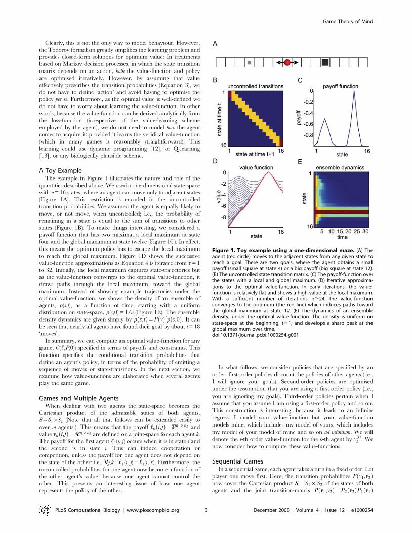
A Toy ExampleThe example in Figure 1 illustrates the nature and role of the

quantities described above. We used a one-dimensional state-space

with n = 16 states, where an agent can move only to adjacent states

(Figure 1A). This restriction is encoded in the uncontrolled

transition probabilities. We assumed the agent is equally likely to

move, or not move, when uncontrolled; i.e., the probability of

remaining in a state is equal to the sum of transitions to other

states (Figure 1B). To make things interesting, we considered a

payoff function that has two maxima; a local maximum at state

four and the global maximum at state twelve (Figure 1C). In effect,

this means the optimum policy has to escape the local maximum

to reach the global maximum. Figure 1D shows the successive

value-function approximations as Equation 4 is iterated from t = 1

to 32. Initially, the local maximum captures state-trajectories but

as the value-function converges to the optimal value-function, it

draws paths through the local maximum, toward the global

maximum. Instead of showing example trajectories under the

optimal value-function, we shows the density of an ensemble of

agents, r(s,t), as a function of time, starting with a uniform

distribution on state-space, r(s,0) = 1/n (Figure 1E). The ensemble

density dynamics are given simply by r s,tð Þ~P vð Þtr s,0ð Þ. It can

be seen that nearly all agents have found their goal by about t = 18

‘moves’.

In summary, we can compute an optimal value-function for any

game, G(,,P(0)) specified in terms of payoffs and constraints. This

function specifies the conditional transition probabilities that

define an agent’s policy, in terms of the probability of emitting a

sequence of moves or state-transitions. In the next section, we

examine how value-functions are elaborated when several agents

play the same game.

Games and Multiple AgentsWhen dealing with two agents the state-space becomes the

Cartesian product of the admissible states of both agents,

S = S16S2 (Note that all that follows can be extended easily to

over m agents.). This means that the payoff ‘k i,jð Þ~<n1|n2 and

value vk i,jð Þ~<n1|n2 are defined on a joint-space for each agent k.

The payoff for the first agent ,1(i, j) occurs when it is in state i and

the second is in state j. This can induce cooperation or

competition, unless the payoff for one agent does not depend on

the state of the other: i.e., ;j,k : ,1(i, j) = ,1(i, k). Furthermore, the

uncontrolled probabilities for one agent now become a function of

the other agent’s value, because one agent cannot control the

other. This presents an interesting issue of how one agent

represents the policy of the other.

In what follows, we consider policies that are specified by an

order: first-order policies discount the policies of other agents (i.e.,

I will ignore your goals). Second-order policies are optimised

under the assumption that you are using a first-order policy (i.e.,

you are ignoring my goals). Third-order policies pertain when I

assume that you assume I am using a first-order policy and so on.

This construction is interesting, because it leads to an infinite

regress: I model your value-function but your value-function

models mine, which includes my model of yours, which includes

my model of your model of mine and so on ad infinitum. We will

denote the i-th order value-function for the k-th agent by við Þ

k . We

now consider how to compute these value-functions.

Sequential GamesIn a sequential game, each agent takes a turn in a fixed order. Let

player one move first. Here, the transition probabilities P v1,v2ð Þnow cover the Cartesian product S~S1|S2 of the states of both

agents and the joint transition-matrix P v1,v2ð Þ~P2 v2ð ÞP1 v1ð Þ

Figure 1. Toy example using a one-dimensional maze. (A) Theagent (red circle) moves to the adjacent states from any given state toreach a goal. There are two goals, where the agent obtains a smallpayoff (small square at state 4) or a big payoff (big square at state 12).(B) The uncontrolled state transition matrix. (C) The payoff-function overthe states with a local and global maximum. (D) Iterative approxima-tions to the optimal value-function. In early iterations, the value-function is relatively flat and shows a high value at the local maximum.With a sufficient number of iterations, t$24, the value-functionconverges to the optimum (the red line) which induces paths towardthe global maximum at state 12. (E) The dynamics of an ensembledensity, under the optimal value-function. The density is uniform onstate-space at the beginning, t = 1, and develops a sharp peak at theglobal maximum over time.doi:10.1371/journal.pcbi.1000254.g001

Game Theory of Mind


factorises into agent-specific terms. These are given by

P1 v1ð Þij~P1 0ð Þijexp ~vv1 ið Þð ÞP

k

P1 0ð Þkjexp ~vv1 kð Þð Þ

P2 v2ð Þij~P2 0ð Þijexp ~vv2 ið Þð ÞP

k

P2 0ð Þkjexp ~vv2 kð Þð Þ

P1 0ð Þ~I6P1 0ð Þ

P2 0ð Þ~P2 0ð Þ6I

ð5Þ

where Pk(0) specifies uncontrolled transitions in the joint-space,

given the uncontrolled transitions Pk(0) in the space of the k-th agent.

Their construction using the Kronecker tensor product fl ensures

that the transition of one agent does not change the state of the

other. Furthermore, it assumes that the uncontrolled transitions of

one agent do not depend on the state of the other; they depend only

on the uncontrolled transitions Pk(0) among the k-th agent’s states.

The row vectors~vvk~vec vkð Þ are the vectorised versions of the two

dimensional value-functions for the k-th agent, covering the joint

states. We will use a similar notation for the payoffs, ~‘‘k~vec ‘kð Þ.Critically, both agents have a value-function on every joint-state but

can only change their own state. These value-functions can now be

evaluated through recursive solutions of the Bellman equations

~vv1ð Þ

1 ~~‘‘1z~vv1ð Þ

1 P v1ð Þ

1 ,0� �

~vv1ð Þ

2 ~~‘‘2z~vv1ð Þ

2 P 0,v1ð Þ

2

� �

..

.

~vvið Þ

1 ~~‘‘1z~vvið Þ

1 P við Þ

1 ,vi{1ð Þ

2

� �

~vvið Þ


2 P vi{1ð Þ

1 ,við Þ

2

� �

ð6Þ

This provides a simple way to evaluate the optimal value-functions

for both agents, to any arbitrary order. The optimal value-function

for the first agent, when the second is using við Þ

2 is viz1ð Þ

1 . Similarly,

the optimal value under við Þ

1 for the second is viz1ð Þ

2 . It can be seen

that under an optimum strategy (i.e., a second-level policy) each

agent should increase its order over the other until a QRE obtains

when við Þ

k &viz1ð Þ

k for both agents. However, it is interesting to

consider equilibria under non-optimal strategies, when both agents

use low-order policies in the mistaken belief that the other agent is

using an even lower order. It is easy to construct examples where

low-order strategies result in risk-dominant policies, which turn into

payoff-dominant policies as high-order strategies are employed; as

illustrated next.

A Stag-HuntIn this example, we used a simple two-player stag-hunt game

where two hunters can either jointly hunt a stag or pursue a rabbit

independently [14]. Table 1 provides the respective payoffs for this

game as a normal form representation. If an agent hunts a stag, he

must have the cooperation of his partner in order to succeed. An

agent can catch a rabbit by himself, but a rabbit is worth less than

a stag. This furnishes two pure-strategy equilibria: one is risk-

dominant with low-payoff states that can be attained without

cooperation (i.e., catching a rabbit) and the other is payoff

dominant; high-payoff states that require cooperation (i.e.,

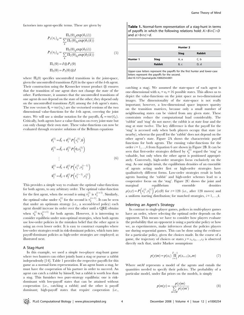
catching a stag). We assumed the state-space of each agent is

one-dimensional with n1 = n2 = 16 possible states. This allows us to

depict the value-functions on the joint space as two-dimensional

images. The dimensionality of the state-space is not really

important; however, a low-dimensional space imposes sparsity

on the transition matrices, because only a small number of

neighbouring states can be visited from any given state. These

constraints reduce the computational load considerably. The

‘rabbit’ and ‘stag’ do not move; the rabbit is at state four and the

stag at state twelve. The key difference is that the payoff for the

‘stag’ is accessed only when both players occupy that state (or

nearby), whereas the payoff for the ‘rabbit’ does not depend on the

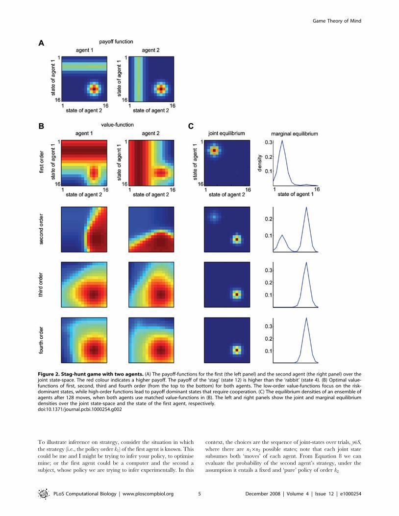
other agent’s state. Figure 2A shows the characteristic payoff

functions for both agents. The ensuing value-functions for the

order i = 1,…,4 from Equation 6 are shown in Figure 2B. It can be

seen that first-order strategies defined by v1ð Þ

k regard the ‘stag’ as

valuable, but only when the other agent is positioned appropri-

ately. Conversely, high-order strategies focus exclusively on the

stag. As one might intuit, the equilibrium densities of an ensemble

of agents acting under first or high-order strategies have

qualitatively different forms. Low-order strategies result in both

agents hunting the ‘rabbit’ and high-order schemes lead to a

cooperative focus on the ‘stag’. Figure 2C shows the joint and

marginal equilibrium ensemble densities

r s,tð Þ~P við Þ

1 ,við Þ

2

� �t

r s,0ð Þ for t = 128 (i.e., after 128 moves) and

a uniform starting distribution; for matched strategies, i = 1,…,4.

Inferring an Agent’s StrategyIn contrast to single-player games, polices in multi-player games

have an order, where selecting the optimal order depends on the

opponent. This means we have to consider how players evaluate

the probability that an opponent is using a particular policy or how

we, as experimenters, make inferences about the policies players

use during sequential games. This can be done using the evidence

for a particular policy, given the choices made. In the course of a

game, the trajectory of choices or states y = s1,s2,…,sT is observed

directly such that, under Markov assumptions

p y mjð Þ~p s1ð Þ PT{1

t~1p stz1 st,mjð Þ ð7Þ

Where mMM represents a model of the agents and entails the

quantities needed to specify their policies. The probability of a

particular model, under flat priors on the models, is simply

p m yjð Þ~ p y mjð ÞPm’[M

p y m’jð Þ ð8Þ

Table 1. Normal-form representation of a stag-hunt in termsof payoffs in which the following relations hold: A.B$C.Dand a.b$c.d.

Hunter 2

Stag Rabbit

Hunter 1 Stag A, a C, b

Rabbit B, c D, d

Upper-case letters represent the payoffs for the first hunter and lower-caseletters represent the payoffs for the second.doi:10.1371/journal.pcbi.1000254.t001

Game Theory of Mind


To illustrate inference on strategy, consider the situation in which

the strategy (i.e., the policy order k1) of the first agent is known. This

could be me and I might be trying to infer your policy, to optimise

mine; or the first agent could be a computer and the second a

subject, whose policy we are trying to infer experimentally. In this

context, the choices are the sequence of joint-states over trials, yMS,

where there are n16n2 possible states; note that each joint state

subsumes both ‘moves’ of each agent. From Equation 8 we can

evaluate the probability of the second agent’s strategy, under the

assumption it entails a fixed and ‘pure’ policy of order k2

Figure 2. Stag-hunt game with two agents. (A) The payoff-functions for the first (the left panel) and the second agent (the right panel) over thejoint state-space. The red colour indicates a higher payoff. The payoff of the ‘stag’ (state 12) is higher than the ‘rabbit’ (state 4). (B) Optimal value-functions of first, second, third and fourth order (from the top to the bottom) for both agents. The low-order value-functions focus on the risk-dominant states, while high-order functions lead to payoff dominant states that require cooperation. (C) The equilibrium densities of an ensemble ofagents after 128 moves, when both agents use matched value-functions in (B). The left and right panels show the joint and marginal equilibriumdensities over the joint state-space and the state of the first agent, respectively.doi:10.1371/journal.pcbi.1000254.g002

Game Theory of Mind


p k2 y,k1jð Þ~ p y k1,k2jð ÞPk’2[M

p y k1,k’2jð Þ

p y k1,k2jð Þ~p s1ð ÞPt

p stz1 st,k1,k2jð Þ

p stz1~i st~j,k1,k2jð Þ~P vk1ð Þ

1 ,vk2ð Þ

2

� �ij

ð9Þ

Here, the model is specified by the unknown policy order, m = k2 of

the second agent. Equation 9 uses the joint transition probabilities

on the moves of all players; however, one gets exactly the same

result using just the moves and transition matrix from the player in

question. This is because, the contributions of the other players

cancel, when the evidence is normalised. We use the redundant

form in Equation 9 so that it can be related more easily to inference

on the joint strategies of all agents in Equation 8. An example of this

inference is provided in Figure 3. In Figure 3A and 3B, we used

unmatched and matched strategies to generate samples using the

probability transition matrices P v4ð Þ

1 ,v1ð Þ

2

� �and P v

4ð Þ1 ,v

4ð Þ2

� �;

starting in the first state (i.e., both agents in state 1) respectively.

These simulated games comprised four consecutive 32-move trials

of the stag-hunt game specified in Figure 2. The ensuing state

trajectories are shown in the left panels. We then inverted the

sequence using Equation 9 and a model-space of

M~k’2~ 1, . . . ,4f g. The results for T = 1,…,128 are shown in

the right panels. For both simulations, the correct strategy discloses

itself after about sixty moves, in terms of conditional inference on

the second agent’s policy. It takes this number of trials because,

initially, the path in joint state-space is ambiguous; as it moves

towards both the rabbit and stag.

Bounded RationalityWe have seen how an N-player game is specified completely by

a set of utility functions and a set of constraints on state-transitions.

These two quantities define, recursively, optimal value-functions,

vkð Þ

1 , . . . ,vkð Þ

N

n oof increasing order and their implicit policies.

Given these policies, one can infer the strategies employed by

agents, in terms of which policies they are using, given a sequence

of transitions. In two-player games, when the opponent uses policy

k, the optimum strategy is to use policy k+1. This formulation

accounts for the representation of another’s goals and optimising

both policies and strategies. However, it induces a problem; to

optimise ones own strategy, one has to know the opponent’s

policy. Under rationality assumptions, this is not really a problem

because rational players will, by induction, use policies of

sufficiently high order to ensure vkð Þ

i &vkz1ð Þ

i . This is because

each player will use a policy with an order that is greater than the

opponent and knows a rational opponent will do the same. The

interesting issues arise when we consider bounds or constraints on

the strategies available to each player and their prior expectations

about these constraints.

Here, we deal with optimisation under bounded rationality [4]

that obliges players to make inferences about each other. We

consider bounds, or constraints, that lead to inference on the

opponent’s strategy. As intimated above, it is these bounds that

lead to interesting interactions between players and properly

accommodate the fact that real players do not have unbounded

computing resources to attain a QRE by using v?ð Þ

i . These

constraints are formulated in terms of the policy ki of the i-th

player, which specifies the corresponding value-function and

policy Pi vkið Þ

i

� �. The constraints we consider are:

N The i-th player uses an approximate conditional density qi(kj)

on the strategy of the j-th player that is a point mass at the

conditional mode, kij .

N Each player has priors pi(kj), which place an upper bound on

the opponents sophistication; ;kj.Ki : pi(kj) = 0

These assumptions have a number of important implications.

First, because qi(kj) is a point mass at the mode kij , each player will

Figure 3. Inference on agent’s strategy in the stag-hunt game. We assumed agents used unmatched strategies, in which the first agent useda fourth order strategy and the second agent used a first order strategy (A), and matched strategies - both agents used the fourth order strategy (B).The left panels show four state trajectories of 32 moves simulated using (or generated from) value-functions in Figure 2B. The right panels show theconditional probabilities of the second agent’s strategy over a model-space of k’2~ 1, . . . ,4f g as a function of time.doi:10.1371/journal.pcbi.1000254.g003

Game Theory of Mind


assume every other player is using a pure strategy, as opposed to a

strategy based on a mixture of value-functions. Second, under this

assumption, each player will respond optimally with another pure

strategy, ki~kijz1. Third, because there is an upper bound on

kijƒKi imposed by an agent’s priors, they will never call upon

strategies more sophisticated than ki = Ki+1. In this way, Ki bounds

both the prior assumptions about other players and the

sophistication of the player per se. This defines a ‘type’ of player

[15] and is the central feature of the bounded rationality under

which this model is developed. Critically, type is an attribute of a

player’s prior assumptions about others. The nature of this bound

means that any player cannot represent the goals or intentions of

another player who is more sophisticated; in other words, it

precludes any player ‘knowing the mind of God’ [16].

Representing the Goals of AnotherUnder flat priors on the bounded support of the priors pi(kj), the

mode can be updated with each move using Equation 9. Here,

player one would approximate the conditional density on the

opponent’s strategy with the mode

k12 tð Þ~ arg max

k2[ 1,...,K1f gp k2 tð Þ y,k1jð Þ

p k2 Tð Þ y,k1jð Þ!p y 1, . . . ,Tð Þ k1 1, . . . ,Tð Þ,k2jð Þp1 k2ð Þ

~p s1ð Þ PT{1

t~1p stz1 st,k1 tð Þ,k2jð Þ

ð10Þ

And optimise its strategy accordingly, by using

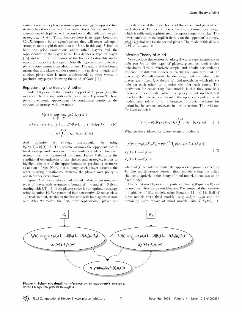
k1 tz1ð Þ~k12 tð Þz1. This scheme assumes the opponent uses a

fixed strategy and consequently accumulates evidence for each

strategy over the duration of the game. Figure 4 illustrates the

conditional dependencies of the choices and strategies; it tries to

highlight the role of the upper bounds in precluding recursive

escalation of ki(t). Note, that although each player assumes the

other is using a stationary strategy, the players own policy is

updated after every move.

Figure 5A shows a realization of a simulated stag-hunt using two

types of player with asymmetric bounds K1 = 4 and K2 = 3 (both

starting with ki(1) = 1). Both players strive for an optimum strategy

using Equation 10. We generated four consecutive 32-move trials;

128 trials in total, starting in the first state with both agents in state

one. After 20 moves, the first, more sophisticated, player has

properly inferred the upper bound of the second and plays at one

level above it. The second player has also optimised its strategy,

which is sufficiently sophisticated to support cooperative play. The

lower panels show the implicit density on the opponent’s strategy,

p(k2|y,k1); similarly for the second player. The mode of this density

is k12 in Equation 10.

Inferring Theory of MindWe conclude this section by asking if we, as experimenters, can

infer post hoc on the ‘type’ of players, given just their choice

behaviours. This is relatively simple and entails accumulating

evidence for different models in exactly the same way that the

players do. We will consider fixed-strategy models in which both

players use a fixed ki or theory of mind models, in which players

infer on each other, to optimise ki(t) after each move. The

motivation for considering fixed models is that they provide a

reference model, under which the policy is not updated and

therefore there is no need to infer the opponent’s policy. Fixed

models also relate to an alternative [prosocial] scheme for

optimising behaviour, reviewed in the discussion. The evidence

for fixed models is

p y mjð Þ~p y k1,k2jð Þ~p s1ð Þ PT{1

t~1p stz1 st,k1,k2jð Þ ð11Þ

Whereas the evidence for theory of mind models is

p y mjð Þ~p y K1,K2jð Þ~p s1ð Þ PT{1

t~1p stz1 st,k1 tð Þ,k2 tð Þjð Þ

k1 tz1ð Þ~k12 tð Þz1

k2 tz1ð Þ~k21 tð Þz1

ð12Þ

where ki2 tð Þ are inferred under the appropriate priors specified by

Ki. The key difference between these models is that the policy

changes adaptively in the theory of mind model, in contrast to the

fixed model.

Under flat model priors, the posterior, p(mi|y) (Equation 8) can

be used for inference on model-space. We computed the posterior

probabilities of fifty models, using Equation 11 and 12. Half of

these models were fixed models using k1,k2 = 1,…,5 and the

remaining were theory of mind models with K1,K2 = 0,…,4.

Figure 4. Schematic detailing inference on an opponent’s strategy.doi:10.1371/journal.pcbi.1000254.g004

Game Theory of Mind


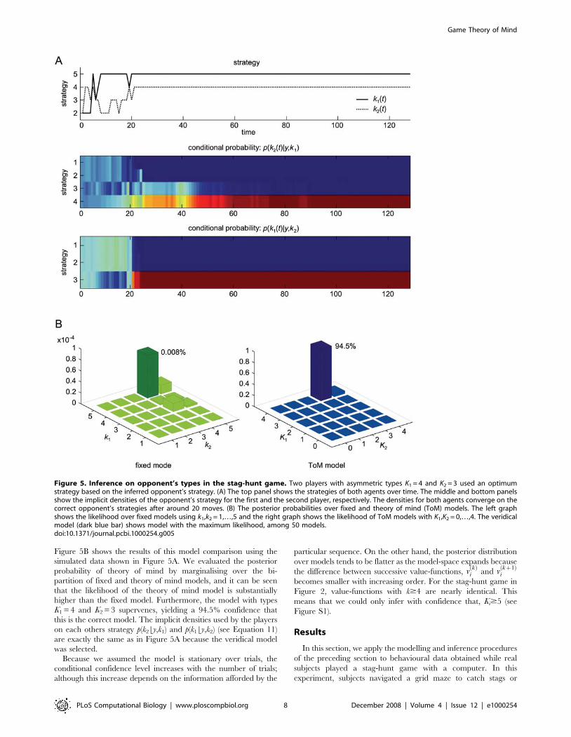
Figure 5B shows the results of this model comparison using the

simulated data shown in Figure 5A. We evaluated the posterior

probability of theory of mind by marginalising over the bi-

partition of fixed and theory of mind models, and it can be seen

that the likelihood of the theory of mind model is substantially

higher than the fixed model. Furthermore, the model with types

K1 = 4 and K2 = 3 supervenes, yielding a 94.5% confidence that

this is the correct model. The implicit densities used by the players

on each others strategy p(k2|y,k1) and p(k1|y,k2) (see Equation 11)

are exactly the same as in Figure 5A because the veridical model

was selected.

Because we assumed the model is stationary over trials, the

conditional confidence level increases with the number of trials;

although this increase depends on the information afforded by the

particular sequence. On the other hand, the posterior distribution

over models tends to be flatter as the model-space expands because

the difference between successive value-functions, vkð Þ

i and vkz1ð Þ

i

becomes smaller with increasing order. For the stag-hunt game in

Figure 2, value-functions with k$4 are nearly identical. This

means that we could only infer with confidence that, Ki$5 (see

Figure S1).

Results

In this section, we apply the modelling and inference procedures

of the preceding section to behavioural data obtained while real

subjects played a stag-hunt game with a computer. In this

experiment, subjects navigated a grid maze to catch stags or

Figure 5. Inference on opponent’s types in the stag-hunt game. Two players with asymmetric types K1 = 4 and K2 = 3 used an optimumstrategy based on the inferred opponent’s strategy. (A) The top panel shows the strategies of both agents over time. The middle and bottom panelsshow the implicit densities of the opponent’s strategy for the first and the second player, respectively. The densities for both agents converge on thecorrect opponent’s strategies after around 20 moves. (B) The posterior probabilities over fixed and theory of mind (ToM) models. The left graphshows the likelihood over fixed models using k1,k2 = 1,…,5 and the right graph shows the likelihood of ToM models with K1,K2 = 0,…,4. The veridicalmodel (dark blue bar) shows model with the maximum likelihood, among 50 models.doi:10.1371/journal.pcbi.1000254.g005

Game Theory of Mind


rabbits. When successful, subjects accrued points that were

converted into money at the end of the experiment. First, we

inferred the model used by subjects, under the known policies of

their computer opponents. This allowed us to establish whether

they were using theory of mind or fixed models and, under theory

of mind models, how sophisticated the subjects were. Using

Equation 10 we then computed the subjects’ conditional densities

on the opponent’s strategies, under their maximum a posteriori

sophistication.

Experimental ProceduresThe subject’s goal was to negotiate a two-dimensional grid maze in

order to catch a stag or rabbit (Figure 6). There was one stag and two

rabbits. The rabbits remained at the same grid location and

consequently were easy to catch without help from the opponent. If

one hunter moved to the same location as a rabbit, he/she caught the

rabbit and received ten points. In contrast, the stag could move to

escape the hunters. The stag could only be caught if both hunters

moved to the locations adjacent to the stag (in a co-operative pincer

movement), after which they both received twenty points. Note that

as the stag could escape optimally, it was impossible for a hunter to

catch the stag alone. The subjects played the game with one of two

types of computer agents; A and B. Agent A adopted a lower-order

(competitive) strategy and tried to catch a rabbit by itself, provided

both hunters were not close to the stag. On the other hand, agent B

used a higher-order (cooperative) strategy and chased the stag even if

it was close to a rabbit. At each trial, both hunters and the stag moved

one grid location sequentially; the stag moved first, the subject moved

next, and the computer moved last. The subjects chose to move to

one of four adjacent grid locations (up, down, left, or right) by pressing

a button; after which they moved to the selected grid. Each move

lasted two seconds and if the subjects did not press a key within this

period, they remained at the same location until the next trial.

Subjects lost one point on each trial (even if they did not move).

Therefore, to maximise the total number of points, it was worth

trying to catch a prey as quickly as possible. The round finished

when either of the hunters caught a prey or when a certain number

of trials (1565) had expired. To prevent subjects changing their

behaviour, depending on the inferred number of moves remaining,

the maximum number of moves was randomised for each round. In

practice, this manipulation was probably unnecessary because the

minimum number of moves required to catch a stag was at most

nine (from any initial state). Furthermore, the number of ‘time out’

rounds was only four out of a total 240 rounds (1.7%). At the

beginning of each round the subjects were given fifteen points,

which decreased by one point per trial, continuing below zero

beyond fifteen trials. For example, if the subject caught a rabbit on

trial five, he/she got the ten points for catching the rabbit, plus the

remaining time points: 10 = 1525 points, giving 20 points in total,

whereas the other player received only their remaining time points;

i.e., 10 points. If the hunters caught a stag at trial eight, both

received the remaining 7 = 1528 time points plus 20 points for

catching the stag, giving 27 points in total. The remaining time

points for both hunters were displayed on each trial and the total

number of points accrued was displayed at the end of each round.

We studied six (normal young) subjects (three males) and each

played four blocks with both types of computer agent in

alternation. Each block comprised ten rounds; so that they played

forty rounds in total. The start positions of all agents; the hunters

and the stag, were randomised on every round, under the

constraint that the initial distances between each hunter and the

stag were more than four grids points.

Modelling Value FunctionsWe applied our theory of mind model to compute the optimal

value-functions for the hunters and stag. As hunters should

Figure 6. Stag-hunt game with two hunters: a human subject and a computer agent. The aim of the hunters (red and green circles) is tocatch stag (big square) or rabbit (small squares). The hunters and the stag can move to adjacent states, while the rabbits are stationary. At each trial,both hunters and the stag move sequentially; the stag moved first, the subject moved next, and the computer moved last. Each round finishes wheneither of the hunters caught a prey or when a maximum number of moves had expired.doi:10.1371/journal.pcbi.1000254.g006

Game Theory of Mind


optimise their strategies based not only on the other hunter’s

behaviour but also the stag’s, we modelled the hunt as a game with

three agents; two hunters and a stag. Here state-space became the

Cartesian product of the admissible states of all agents, and the

payoff was defined on a joint space for each agent; i.e., on a

|S1|6|S2|6|S3| array. The payoff for the stag was minus one

when both hunters were at the same location as the stag and zero

for the other states. For the hunters, the payoff of catching a stag

was one and accessed only when both the hunters’ states were next

to the stag. The payoff for catching a rabbit was one half and did

not depend on the other hunter’s state. For the uncontrolled

transition probabilities, we assumed that all agents would choose

allowable actions (including no-move) with equal probability and

allowed co-occupied locations; i.e., two or more agents could be in

the same state. Allowable moves were constrained by obstacles in

the maze (see Figure 6).

We will refer to the stag, subject, and computer as the 1st, 2nd,

and 3rd agent, respectively. The transition probability at each trial

is P~P3 v3ð ÞP2 v2ð ÞP1 v1ð Þ. The i-th order value-function for the

j-th agent, við Þ

j , was evaluated through recursive solutions of the

Bellman equations by generalising Equation 6 to three players

~vv1ð Þ

1 ~~‘‘1z~vv1ð Þ

1 P v1ð Þ

1 ,0,0� �

~vvið Þ


2 P v1ð Þ

1 ,við Þ

2 ,vi{1ð Þ

3

� �

~vvið Þ


3 P v1ð Þ

1 ,vi{1ð Þ

2 ,við Þ

3

� �ð13Þ

Notice that the first agent’s (stag’s) value-function is fixed at first-

order. This is because we assumed that the hunters believed,

correctly, that the stag was not sophisticated. We used a

convergence criterion of vt{1 { vtj j1�

vt{1j j1 v exp{10 to

calculate the optimal value-functions, using Equation 4. For

simplicity, we assumed the sensitivity l of each player was one. A

maximum likelihood estimation of the subjects’ sensitivities, using

the observed choices from all subjects together, showed that the

optimal value was l = 1.6. Critically, the dependency of the

likelihood on strategy did not change much with sensitivity, which

means our inferences about strategy are fairly robust to deviations

from l = 1 (see Figure S2). When estimated individually for each

subject, the range was 1.5#l#1.8, suggesting our approximation

was reasonable and enabled us to specify the policy for each value-

function and solve Equation 13 recursively.

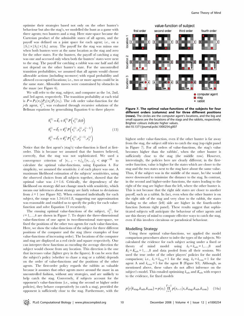
The ensuing optimal value-functions of the subject, við Þ

2 , for

i = 1,…,4 are shown in Figure 7. To depict the three-dimensional

value-functions of one agent in two-dimensional state-space, we

fixed the positions of the other two agents for each value-function.

Here, we show the value-functions of the subject for three different

positions of the computer and the stag (three examples of four

value-functions of increasing order). The locations of the computer

and stag are displayed as a red circle and square respectively. One

can interpret these functions as encoding the average direction the

subject would choose from any location. This direction is the one

that increases value (lighter grey in the figures). It can be seen that

the subject’s policy (whether to chase a stag or a rabbit) depends

on the order of value-functions and the positions of the other

agents. The first-order policy regards the rabbits as valuable

because it assumes that other agents move around the maze in an

uncontrolled fashion, without any strategies, and are unlikely to

help catch the stag. Conversely, if subjects account for the

opponent’s value-functions (i.e., using the second or higher order

policies), they behave cooperatively (to catch a stag), provided the

opponent is sufficiently close to the stag. Furthermore, with the

highest order value-function, even if the other hunter is far away

from the stag, the subject still tries to catch the stag (top right panel

in Figure 7). For all orders of value-functions, the stag’s value

becomes higher than the rabbits’, when the other hunter is

sufficiently close to the stag (the middle row). However,

interestingly, the policies here are clearly different; in the first-

order function, value is higher for the states which are closer to the

stag and the two states next to the stag have about the same value.

Thus, if the subject was in the middle of the maze, he/she would

move downward to minimize the distance to the stag. In contrast,

in the second and higher-order functions, the states leading to the

right of the stag are higher than the left, where the other hunter is.

This is not because that the right side states are closer to another

payoff, such as a rabbit. In fact, even when the other hunter is on

the right side of the stag and very close to the rabbit, the states

leading to the other (left) side are higher in the fourth-order

function (bottom right panel). These results suggest that sophis-

ticated subjects will anticipate the behaviour of other agents and

use this theory of mind to compute effective ways to catch the stag,

even if this involves circuitous or paradoxical behaviour.

Modelling StrategyUsing these optimal value-functions, we applied the model

comparison procedures above to infer the types of the subjects. We

calculated the evidence for each subject acting under a fixed or

theory of mind model using k2 = ksub = 1,…,8 and

K2 = Ksub = 1,…,8 and data pooled from all their sessions. We

used the true order of the other players’ policies for the model

comparison; i.e., k1 = kstag = 1 for the stag, k3 = kcom = 1 for the

agent A and kcom = 5 for the agent B (Figure S3). Although, as

mentioned above, these values do not affect inference on the

subject’s model. This entailed optimising ksub and Ksub with respect

to the evidence, for fixed models

p y kstag,ksub,kcom

�� ~p s1ð Þ P

T{1

t~1p stz1 st,kstag,ksub,kcom

�� ð14aÞ

Figure 7. The optimal value-functions of the subjects for fourdifferent orders (columns) and for three different positions(rows). The circles are the computer agent’s locations, and the big andsmall squares are the locations of the stags and the rabbits, respectively.Brighter colours indicate higher values.doi:10.1371/journal.pcbi.1000254.g007

Game Theory of Mind


and theory of mind models

p y kstag,Ksub,kcom

�� ~p s1ð Þ P

T{1

t~1p stz1 st,kstag,ksub tð Þ,kcom

��

ksub tð Þ~ksubcom t{1ð Þz1

ð14bÞ

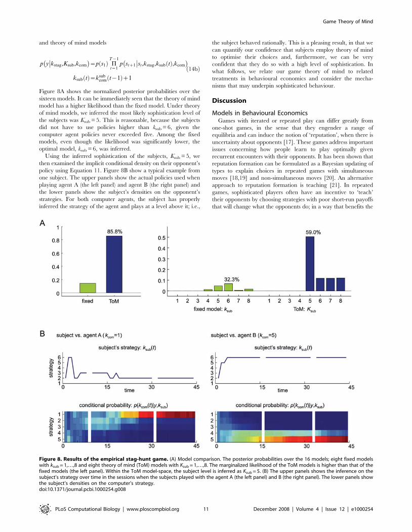
Figure 8A shows the normalized posterior probabilities over the

sixteen models. It can be immediately seen that the theory of mind

model has a higher likelihood than the fixed model. Under theory

of mind models, we inferred the most likely sophistication level of

the subjects was Ksub = 5. This is reasonable, because the subjects

did not have to use policies higher than ksub = 6, given the

computer agent policies never exceeded five. Among the fixed

models, even though the likelihood was significantly lower, the

optimal model, ksub = 6, was inferred.

Using the inferred sophistication of the subjects, Ksub = 5, we

then examined the implicit conditional density on their opponent’s

policy using Equation 11. Figure 8B show a typical example from

one subject. The upper panels show the actual policies used when

playing agent A (the left panel) and agent B (the right panel) and

the lower panels show the subject’s densities on the opponent’s

strategies. For both computer agents, the subject has properly

inferred the strategy of the agent and plays at a level above it; i.e.,

the subject behaved rationally. This is a pleasing result, in that we

can quantify our confidence that subjects employ theory of mind

to optimise their choices and, furthermore, we can be very

confident that they do so with a high level of sophistication. In

what follows, we relate our game theory of mind to related

treatments in behavioural economics and consider the mecha-

nisms that may underpin sophisticated behaviour.

Discussion

Models in Behavioural EconomicsGames with iterated or repeated play can differ greatly from

one-shot games, in the sense that they engender a range of

equilibria and can induce the notion of ‘reputation’, when there is

uncertainty about opponents [17]. These games address important

issues concerning how people learn to play optimally given

recurrent encounters with their opponents. It has been shown that

reputation formation can be formulated as a Bayesian updating of

types to explain choices in repeated games with simultaneous

moves [18,19] and non-simultaneous moves [20]. An alternative

approach to reputation formation is teaching [21]. In repeated

games, sophisticated players often have an incentive to ‘teach’

their opponents by choosing strategies with poor short-run payoffs

that will change what the opponents do; in a way that benefits the

Figure 8. Results of the empirical stag-hunt game. (A) Model comparison. The posterior probabilities over the 16 models; eight fixed modelswith ksub = 1,…,8 and eight theory of mind (ToM) models with Ksub = 1,…,8. The marginalized likelihood of the ToM models is higher than that of thefixed models (the left panel). Within the ToM model-space, the subject level is inferred as Ksub = 5. (B) The upper panels shows the inference on thesubject’s strategy over time in the sessions when the subjects played with the agent A (the left panel) and B (the right panel). The lower panels showthe subject’s densities on the computer’s strategy.doi:10.1371/journal.pcbi.1000254.g008

Game Theory of Mind


sophisticated player in the long run. Indeed, Camerer et al [22]

showed that strategic teaching in their EWA model could select

one of many repeated-game equilibria and give rise to reputation

formation without updating of types. The crucial difference

between these approaches is that in the type-based model,

reputation is the attribute of a particular player, while in the

teaching model, a strategy attains a reputation. In our approach,

types are described in terms of bounds on strategy; the

sophistication level. This contrasts with treatments that define

types in terms of unobserved payoff functions, which model

strategic differences using an attribute of the agent; e.g., normal or

honest type.

Recursive or hierarchical approaches to multi-player games

have been adopted in behavioural economics [23,24] and artificial

intelligence [25], in which individual decision policies systemati-

cally exploit embedded levels of inference. For instance, some

studies have assumed that subject’s decisions follow one of a small

set of a priori plausible types, which include non-strategic and

strategic forms. Under these assumptions, inference based on

decisions in one-shot (non-iterated) games suggests that while

policies may be heterogeneous, the level of sophistication may be

equivalent to an approximate value of k; two or three. Camerer

and colleagues [26] have suggested a ‘cognitive hierarchy’ model,

in which subjects generate a form of cognitive hierarchy over each

other’s level of reciprocal thinking. In this model ‘k’ corresponds to

the depth of tree-search, and when estimated over a collection of

games such as the p-beauty game, yields values of around one and

a half to two. Note that ‘steps of strategic thinking’ are not the

same as the levels of sophistication in this paper. The

sophistication addressed here pertains to the recursive represen-

tation of an opponent’s goals, and can be applied to any iterated

extensive form game. Despite this, studies in behavioural

economics suggest lower levels of sophistication than ours. One

reason for this may be that most games employed in previous

studies have been one-shot games, which place less emphasis on

planning for future interactions that rest on accurate models of an

opponent’s strategy.

In the current treatment, we are not suggesting that players

actually compute their optimal strategy explicitly; or indeed are

aware of any implicit inference on the opponent’s policy. Our

model is phenomenological and is designed to allow model

comparison and predictions (under any particular model) of brain

states that may encode the quantities necessary to optimize

behaviour. It may be that the mechanisms of this optimization are

at a very low level (e.g., at the level of synaptic plasticity) and have

been shaped by evolutionary pressure. In other words, we do not

suppose that subjects engage in explicit cognitive operations but

are sufficiently tuned to interactions with con-specifics that their

choice behaviour is sophisticated. We now pursue this perspective

from the point of view of evolutionary optimization of the policies

themselves.

Prosocial UtilityHere, we revisit the emergence of cooperative equilibria and ask

whether sophisticated strategies are really necessary. Hitherto, we

have assumed that the utility functions ,i are fixed for any game.

This is fine in an experimental setting but in an evolutionary

setting, ,i may be optimised themselves. In this case, there is a

fundamental equivalence between different types of agents, in

terms of their choices. This is because exactly the same

equilibrium behaviour can result from interaction between

sophisticated agents with empathy (i.e., theory of mind) and

unsophisticated agents with altruistic utility-functions. In what

follows, we show why this is the case:

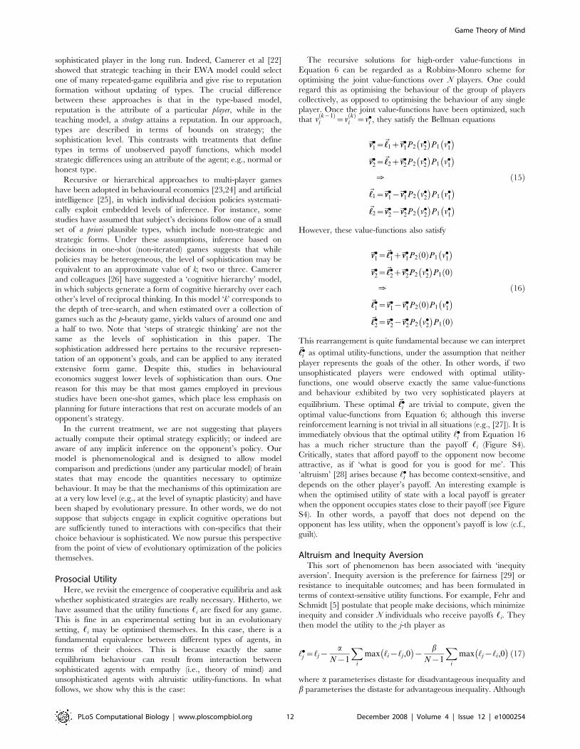
The recursive solutions for high-order value-functions in

Equation 6 can be regarded as a Robbins-Monro scheme for

optimising the joint value-functions over N players. One could

regard this as optimising the behaviour of the group of players

collectively, as opposed to optimising the behaviour of any single

player. Once the joint value-functions have been optimized, such

that vk{1ð Þ

i ~vkð Þ

i ~v.i , they satisfy the Bellman equations

~vv.1~~‘‘1z~vv

.1P2 v.2� �

P1 v.1� �

~vv.2~~‘‘2z~vv

.2P2 v.2� �

P1 v.1� �

[

~‘‘1~~vv.1{~vv

.1P2 v.2� �

P1 v.1� �

~‘‘2~~vv.2{~vv

.2P2 v.2� �

P1 v.1� �

ð15Þ

However, these value-functions also satisfy

~vv.1~~‘‘.1z~vv

.1P2 0ð ÞP1 v.1

� �

~vv.2~~‘‘.2z~vv

.2P2 v.2� �

P1 0ð Þ

[

~‘‘.1~~vv.1{~vv

.1P2 0ð ÞP1 v.1

� �

~‘‘.2~~vv.2{~vv

.2P2 v.2� �

P1 0ð Þ

ð16Þ

This rearrangement is quite fundamental because we can interpret~‘‘.i as optimal utility-functions, under the assumption that neither

player represents the goals of the other. In other words, if two

unsophisticated players were endowed with optimal utility-

functions, one would observe exactly the same value-functions

and behaviour exhibited by two very sophisticated players at

equilibrium. These optimal ~‘‘.i are trivial to compute, given the

optimal value-functions from Equation 6; although this inverse

reinforcement learning is not trivial in all situations (e.g., [27]). It is

immediately obvious that the optimal utility ‘.i from Equation 16

has a much richer structure than the payoff ,i (Figure S4).

Critically, states that afford payoff to the opponent now become

attractive, as if ‘what is good for you is good for me’. This

‘altruism’ [28] arises because ‘.i has become context-sensitive, and

depends on the other player’s payoff. An interesting example is

when the optimised utility of state with a local payoff is greater

when the opponent occupies states close to their payoff (see Figure

S4). In other words, a payoff that does not depend on the

opponent has less utility, when the opponent’s payoff is low (c.f.,

guilt).

Altruism and Inequity AversionThis sort of phenomenon has been associated with ‘inequity

aversion’. Inequity aversion is the preference for fairness [29] or

resistance to inequitable outcomes; and has been formulated in

terms of context-sensitive utility functions. For example, Fehr and

Schmidt [5] postulate that people make decisions, which minimize

inequity and consider N individuals who receive payoffs ,i. They

then model the utility to the j-th player as

‘.j ~‘j{a

N{1

Xi

max ‘i{‘j ,0� �

{b

N{1

Xi

max ‘j{‘i,0� �

ð17Þ

where a parameterises distaste for disadvantageous inequality and

b parameterises the distaste for advantageous inequality. Although

Game Theory of Mind


a compelling heuristic, this utility function is an ad hoc nonlinear

mixture of payoffs and has been critiqued for its rhetorical nature

[30]. An optimal nonlinear mixture is given by substituting

Equation 15 into Equation 16 to give

~‘‘.1~~‘‘1z~vv

.1 P2 v.2

� �{P2 0ð Þ

� �P1 v.1� �

~‘‘.2~~‘‘2z~vv

.2P2 v.2� �

P1 v.1� �

{P1 0ð Þ� � ð18Þ

These equalities express the optimal utility functions in terms of

payoff and a ‘prosocial’ utility (the second terms), which allow

unsophisticated agents to optimise their social exchanges. The

prosocial utility of any state is simply the difference in value

expected after the next move with a sophisticated, relative to an

unsophisticated, opponent. Equation 15 might provide a princi-

pled and quantitative account of inequity aversion, which holds

under rationality assumptions.

One might ask, what is the relevance of an optimised utility

function for game theory? The answer lies in the hierarchal co-

evolution of agents (e.g., [15,31]), where the prosocial part of ‘.imay be subject to selective pressure. In this context, the unit of

selection is not the player but the group of payers involved in a

game (e.g., a mother and offspring). In this context, optimising

‘.~ ‘.1, . . . ,‘.N� �

over a group of unsophisticated players can

achieve exactly the same result (in terms of equilibrium behaviour)

as evolving highly sophisticated agents with theory of mind (c.f.,

[32]). For example, in ethological terms, it is more likely that the

nurturing behaviour of birds is accounted for by selective pressure

on ,N than invoking birds with theory of mind. This speaks to

‘survival of the nicest’ and related notions of prosocial behaviour

(e.g., [33,34]). Selective pressure on prosocial utility simply means,

for example, that the innate reward associated with consummatory

behaviour is supplemented with rewards associated with nursing

behaviour. We have exploited the interaction between innate and

acquired value previously in an attempt to model the neurobiology

of reinforcement learning [35].

In summary, exactly the same equilibrium behaviour can

emerge from sophisticated players with theory of mind, who act

entirely out of self-interest and from unsophisticated players who

have prosocial altruism, furnished by hierarchical optimisation of

their joint-utility function. It is possible that prosocial utility might

produce apparently irrational behaviour, in an experimental

setting, if it is ignored: Gintis [33] reviews the evidence for

empirically identifiable forms of prosocial behaviour in humans,

(strong reciprocity), that may in part explain human sociality. ‘‘A

strong reciprocator is predisposed to cooperate with others and

punish non co-operators, even when this behaviour cannot be

justified in terms of extended kinship or reciprocal altruism’’. In

line with this perspective, provisional fMRI evidence suggests that

altruism may not be a cognitive faculty that engages theory of

mind but is hard-wired and inherently pleasurable, activating

subgenual cortex and septal regions; structures intimately related

to social attachment and bonding in other species [36]. In short,

bounds on the sophistication of agents can be circumvented by

endowing utility with prosocial components, in the context of

hierarchical optimisation.

Critically, the equivalence between prosocial and sophisticated

behaviour is only at equilibrium. This means that prosocially

altruistic agents will adapt the same strategy throughout an

iterated game; however, sophisticated agents will optimise their

strategy on the basis of the opponent’s behaviour, until

equilibrium is attained. These strategic changes make it possible

to differentiate between the two sorts of agents empirically, using

observed responses. To disambiguate between theory of mind

dependent optimisation and prosocial utility it is sufficient to

establish that players infer on each other. This is why we included

fixed models without such inference in our model comparisons of

the preceding sections. In the context of the stag-hunt game

examined here, we can be fairly confident that subjects employed

inference and theory of mind.

Finally, it should be noted that, although a duality in prosocial

and sophisticated equilibria may exist for games with strong

cooperative equilibria, there may be other games in which this is

less clearly the case; where sophisticated agents and unsophisti-

cated altruistic agents diverge in their behaviour. For example, in

some competitive games (such as Cournot duopolys and Stackel-

berg games), a (selfish) understanding the other players response to

payoff (empathy) produces a very different policy than one in

which that payoff is inherently (altruistically) valued.

ConclusionThis paper has introduced a model of ‘theory of mind’ (ToM)

based on optimum control and game theory to provide a ‘game

theory of mind’. We have considered the representations of goals

in terms of value-functions that are prescribed by utility or

rewards. We have shown it is possible to deduce whether players

make inferences about each other and quantify their sophistication

using choices in sequential games. This rests on comparing

generative models of choices with and without inference. Model

comparison was demonstrated using simulated and real data from

a ‘stag-hunt’. Finally, we noted that exactly the same sophisticated

equilibrium behaviour can be achieved by optimising the utility-

function itself, producing unsophisticated but altruistic agents.

This may be relevant ethologically in hierarchal game theory and

co-evolution.

In this paper, we focus on the essentials of the model and its

inversion using behavioural data, such as subject choices in a stag-

hunt. Future work will try to establish the predictive validity of the

model by showing a subject’s type or sophistication is fairly stable

across different games. Furthermore, the same model will be used

to generate predictions about neuronal responses, as measured

with brain imaging, so that we can characterise the functional

anatomy of these implicit processes. In the present model,

although players infer the opponent’s level of sophistication, they

assume the opponents are rational and that their strategies are

pure and fixed. However, the opponent’s strategy could be

inferred under the assumption the opponent was employing ToM

to optimise their strategy. It would be possible to relax the

assumption that the opponent uses a fixed and pure strategy and

test the ensuing model against the current model. However, this

relaxation entails a considerable computational expense (which the

brain may not be in a position to pay). This is because modeling

the opponent’s inference induces an infinite recursion; that we

resolved by specifying the bounds on rationality. Having said this,

to model things like deception, it will be necessary to model

hierarchical representations of not just the goals of another (as in

this paper) but the optimization schemes used to attain those goals

by assuming agent’s represent the opponent’s optimization of a

changing and possibly mixed strategy. This would entail specifying

different bounds to finesse the ensuing infinite recursion. Finally,

although QRE have become the dominant approach to modelling

human behaviour in, e.g., auctions, it remains to be established

that convergence is always guaranteed (c.f., the negative results on

convergence of fictitious play to Nash equilibria).

Recent interest in the computational basis of ToM has

motivated neuroimaging experiments that test the hypothesis that

putative subcomponents of mentalizing might correlate with

cortical brain activity, particularly in regions implicated in ToM

Game Theory of Mind


by psychological studies [37,38]. In particular, Hampton and

colleagues [39] report compelling data that suggest decision values

and update signals are indeed in represented in putative ToM

regions. These parameters were derived from a model based on

‘fictitious play’, which is a simple, non-hierarchical learning model

of two-player inference. This model provided a better account of

choice behaviour, relative to error-based reinforcement learning

alone; providing support for the notion that apparent ToM

behaviour arises from more than prosocial preferences alone.

Clearly, neuroimaging offers a useful method for future explora-

tion of whether key subcomponents of formal ToM models predict

brain activity in ToM regions and may allow one to adjudicate

between competing accounts.

Supporting Information

Figure S1 A. Log [Euclidean] distance between the value-

functions in Figure 2B. B. Inference of opponent’s types using the

same simulated data used in Figure 5. Two players with

asymmetric types K1 = 4 and K2 = 3. The left graph shows the

likelihood over fixed models using k1,k2 = 1,…,6 and the right

graph shows the likelihood of theory of mind models with

K1,K2 = 0,…,5. The veridical model (dark blue bar) showed the

maximum likelihood among 72 models.

Found at: doi:10.1371/journal.pcbi.1000254.s001 (0.63 MB TIF)

Figure S2 Maximum likelihood estimation over the subject’s

type and payoff sensitivity. We used the models using Ksub = 0,…,5

and l= 0.5,…,3.0 and data pooled from all subjects.


Figure S3 Inference of computer agent’s policy: canonical

inference using all subjects’ data (A) and mean and standard

deviation over six subjects (B). The order of agent A’s policy is

inferred as kcom = 1 and the agent B’s order is inferred as kcom = 5.


Figure S4 The left panels show payoff functions for sophisticated

agents who have theory of mind. The right panels show optimal

utility functions for unsophisticated agents who do not represent

opponent’s goal: they assume opponent’s policy is naı̈ve.


Acknowledgments

We are also grateful to Peter Dayan, Debajyori Ray, Jean Daunizeau, and

Ben Seymour for useful discussions and suggestions and to Peter Dayan for

critical comments on the manuscript. We also acknowledge the substantial

guidance and suggestions of our three reviewers.

Author Contributions

Conceived and designed the experiments: WY RJD KJF. Performed the

experiments: WY. Analyzed the data: WY KJF. Contributed reagents/

materials/analysis tools: WY RJD KJF. Wrote the paper: WY RJD KJF.

References

1. Frith U, Frith CD (2003) Development and neurophysiology of mentalizing.

Philos Trans R Soc Lond Ser B Biol Sci 358: 459–473.

2. Premack DG, Woodruff G (1978) Does the chimpanzee have a theory of mind?

Behavioral Brain Sci 1: 515–526.

3. Simon HA (1990) A mechanism for social selection and successful altruism.

Science 250: 1665–1668.

4. Kahneman D (2003) Maps of bounded rationality: psychology for behavioral

economics. Am Econ Rev 93: 1449–1475.

5. Fehr E, Schmidt KM (1999) A theory of fairness, competition, and cooperation.

Q J Econ 114: 817–868.

6. Bellman R (1952) On the theory of dynamic programming. Proc Natl Acad

Sci U S A 38: 716–719.

7. Todorov E (2006) Linearly-solvable Markov decision problems. Adv Neural Inf

Process Syst 19: 1369–1376.

8. Camerer CF (2003) Behavioural studies of strategic thinking in games. Trends

Cogn Sci 7: 225–231.

9. McKelvey R, Palfrey T (1995) Quantal response equilibria for normal form

games. Games Econ Behav 10: 6–38.

10. Haile PA, Hortacsu A, Kosenok G (2008) On the empirical content of quantal

response equilibrium. Am Econ Rev 98: 180–200.

11. Benveniste A, Metivier M, Prourier P (1990) Adaptive Algorithms and Stochastic

Approximations. Berlin: Springer-Verlag.

12. Sutton RS, Barto AG (1981) Toward a modern theory of adaptive networks:

expectation and prediction. Psychol Rev 88: 135–170.

13. Watkins CJCH, Dayan P (1992) Q-Learning. Mach Learn 8: 279–292.

14. Skyrms B (2003) The Stag Hunt and the Evolution and Social Structure.Cambridge, UK: Cambridge University Press.

15. Smith JM (1982) Evolution and the Theory of Games. Cambridge: CambridgeUniversity Press.

16. Davies P (1992) Mind of God: The Scientific Basis for a Rational World. NewYork: Simon & Schuster.

17. Wilson D (1985) An integrated modle of buyer-seller relationship. J Acad MarkSci 23: 335–345.

18. Kreps DM, Wilson R (1982) Reputation and imperfect information. J EconTheory 27: 253–279.

19. Milgrom P, Roberts J (1982) Predation, Reputation, and Entry Deterrence.J Econ Theory 27: 280–312.

20. Fudenberg D, Levine DK (1989) Reputation and equilibrium selection in gameswith a patient player. Econometrica 57: 759–778.

21. Fudenberg D, Levine D (1998) The Theory of Learning in Games. Cambridge,MA: MIT Press.

22. Camerer CF, Ho TH, Chong JK (2002) Sophisticated experience-weightedattraction learning and strategic teaching in repeated games. J Econ Theory 104:

137–188.23. Stahl DO, Wilson PW (1995) On players models of other players - Theory and

experimental-evidence. Games Econ Behav 10: 218–254.24. Costa-Gomes M, Crawford VP, Broseta B (2001) Cognition and behavior in

normal-form games: an experimental study. Econometrica 69: 1193–1235.

25. Gmytrasiewicz PJ, Doshi P (2005) A framework for sequential planning in multi-agent settings. J Artif Intell Res 24: 49–79.

26. Camerer CF, Ho TH, Chong JK (2004) A cognitive hierarchy model of games.Q J Econ 119: 861–898.

27. Ng A, Russell S (2000) Algorithms for inverse reinforcement learning. In:

Proceeding of the 17th International Conference on Machine Learning. SanFrancisco, CA: Morgan Kaufmann Publishers. pp 663–670.

28. Fehr E, Fischbacher U (2003) The nature of human altruism. Nature 425:785–791.

29. Nelson W (2001) Incorporating fairness into game theory and economics:

Comment. The Am Economic Rev 91: 1180–1183.30. Avner S (2005) The rhetoric of inequity aversion. NAJ Econ 8: http://www.

najecon.org/naj/cache/666156000000000612.pdf.31. Traulsen A, Claussen JC, Hauert C (2006) Coevolutionary dynamics in large,

but finite populations. Phys Rev E 74: 011901.32. Smith JM (1974) The theory of games and the evolution of animal conflicts.

J Theor Biol 47: 209–221.

33. Gintis H (2000) Strong reciprocity and human sociality. J Theor Biol 206:169–179.

34. Gintis H, Bowles S, Boyd R, Fehr E (2003) Explaining altruistic behavior inhumans. Evol Hum Behav 24: 153–172.

35. Friston KJ, Tononi G, Reeke GN, Sporns O, Edelman GM (1994) Value-

dependent selection in the brain: simulation in a synthetic neural model.Neuroscience 59: 229–243.

36. Moll J, Krueger F, Zahn R, Pardini M, Oliveira-Souzat R, Grafman J (2006)Human fronto-mesolimbic networks guide decisions about charitable donation.

Proc Natl Acad Sci U S A 103: 15623–15628.37. McCabe K, Houser D, Ryan L, Smith V, Trouard T (2001) A functional

imaging study of cooperation in two-person reciprocal exchange. Proc Natl Acad

Sci U S A 98: 11832–11835.38. Gallagher HL, Jack AI, Roepstorff A, Frith CD (2002) Imaging the intentional

stance in a competitive game. Neuroimage 16: 814–821.39. Hampton AN, Bossaerts P, O’Doherty JP (2008) Neural correlates of

mentalizing-related computations during strategic interactions in humans. Proc

Natl Acad Sci U S A 105: 6741–6746.

Game Theory of Mind


Documents

Game Theory of Mind - fil.ion.ucl.ac.ukkarl/Game Theory of Mind.pdf · Game Theory of Mind Wako Yoshida*, Ray J. Dolan, Karl J. Friston The Wellcome Trust Centre for Neuroimaging,