Game Theory || Cooperative Game Theory Models

Chapter 10Cooperative Game Theory Models

The common features of a cooperative game theory model – like the model of agame with transferable utility in Chap. 9 – include: the abstraction from a detaileddescription of the strategic possibilities of a player; instead, a detailed descriptionof what players and coalitions can attain in terms of outcomes or utilities; solutionconcepts based on strategic considerations and/or considerations of fairness, equity,efficiency, etc.; if possible, an axiomatic characterization of such solution concepts.For instance, one can argue that the core for TU-games is based on strategic con-siderations whereas the Shapley value is based on a combination of efficiency andsymmetry or fairness with respect to contributions. The latter is made precise by anaxiomatic characterization as in Problem 9.13.

In this chapter a few other cooperative game theory models are discussed:bargaining problems in Sect. 10.1, exchange economies in Sect. 10.2, matchingproblems in Sect. 10.3, and house exchange in Sect. 10.4.

10.1 Bargaining Problems

An example of a bargaining problem is the division problem in Sect. 1.3.5. Anoncooperative, strategic approach to such a bargaining problem can be found inSect. 6.7, see also Problems 6.15 and 6.16. In this section we treat the bargainingproblem from a cooperative, axiomatic perspective. Surprisingly, there is a closerelation between this approach and the strategic approach, as we will see below. InSect. 10.1.1 we discuss the Nash bargaining solution and in Sect. 10.1.2 its relationwith the Rubinstein bargaining procedure of Sect. 6.7.

H. Peters, Game Theory – A Multi-Leveled Approach.c© Springer-Verlag Berlin Heidelberg 2008

133

134 10 Cooperative Game Theory Models

10.1.1 The Nash Bargaining Solution

We start with the general definition of a two-person bargaining problem.1

Definition 10.1. A two-person bargaining problem is a pair (S,d), where

(1) S ⊆ R2 is a convex, closed and bounded set.2

(2) d = (d1,d2) ∈ S such that there is some point x = (x1,x2) ∈ S with x1 > d1 andx2 > d2.

S is the feasible set and d is the disagreement point.

The interpretation of a bargaining problem (S,d) is as follows. The two playersbargain over the feasible outcomes in S. If they reach an agreement x = (x1,x2) ∈ S,then player 1 receives utility x1 and player 2 receives utility x2. If they do not reachan agreement, then the game ends in the disagreement point d, yielding utility d1to player 1 and d2 to player 2. Note that this is an interpretation: the bargainingprocedure is not spelled out, so formally there is only the pair (S,d).

For the example in Sect. 1.3.5, the feasible set and the disagreement point aregiven by

S = {x ∈ R2 | 0 ≤ x1,x2 ≤ 1, x2 ≤√

1− x1}, d1 = d2 = 0.

See also Fig. 1.7. In general, a bargaining problem may look as in Fig. 10.1. The setof all such bargaining problems is denoted by B.

Nash [90] raised the following question: for any given bargaining problem (S,d),what is a good compromise? In formal terms, he was looking for a map F : B → R2

which assigns a feasible point to every bargaining problem, i.e., satisfies F(S,d)∈ Sfor every (S,d) ∈ B. Such a map is called a (two-person) bargaining solution.According to Nash, a bargaining solution should satisfy four conditions, namely:

Fig. 10.1 A two-personbargaining problem

d

S

1 We restrict attention here to two-person bargaining problems. For n-person bargaining problemsand, more generally, NTU-games, see Remark 10.3 and Chap. 21.2 A subset of Rk is convex if with each pair of points in the set also the line segment connectingthese points is in the set. A set is closed if it contains its boundary or, equivalently, if for everysequence of points in the set that converges to a point that limit point is also in the set. It is boundedif there is a number M > 0 such that |xi| ≤ M for all points x in the set and all coordinates i.

10.1 Bargaining Problems 135

d

(c)

S T

F(S,d)

F(T,d) dTS

F(T,d) = F(S,d)

(d)

dS

P(S) � F(S,d)

(a)

S

�d

(b)

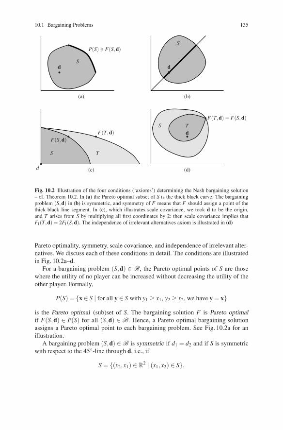
Fig. 10.2 Illustration of the four conditions (‘axioms’) determining the Nash bargaining solution– cf. Theorem 10.2. In (a) the Pareto optimal subset of S is the thick black curve. The bargainingproblem (S,d) in (b) is symmetric, and symmetry of F means that F should assign a point of thethick black line segment. In (c), which illustrates scale covariance, we took d to be the origin,and T arises from S by multiplying all first coordinates by 2: then scale covariance implies thatF1(T,d) = 2F1(S,d). The independence of irrelevant alternatives axiom is illustrated in (d)

Pareto optimality, symmetry, scale covariance, and independence of irrelevant alter-natives. We discuss each of these conditions in detail. The conditions are illustratedin Fig. 10.2a–d.

For a bargaining problem (S,d) ∈ B, the Pareto optimal points of S are thosewhere the utility of no player can be increased without decreasing the utility of theother player. Formally,

P(S) = {x ∈ S | for all y ∈ S with y1 ≥ x1, y2 ≥ x2, we have y = x}

is the Pareto optimal (sub)set of S. The bargaining solution F is Pareto optimalif F(S,d) ∈ P(S) for all (S,d) ∈ B. Hence, a Pareto optimal bargaining solutionassigns a Pareto optimal point to each bargaining problem. See Fig. 10.2a for anillustration.

A bargaining problem (S,d) ∈ B is symmetric if d1 = d2 and if S is symmetricwith respect to the 45◦-line through d, i.e., if

S = {(x2,x1) ∈ R2 | (x1,x2) ∈ S}.


In a symmetric bargaining problem there is no way to distinguish between the play-ers other than by the arbitrary choice of axes. A bargaining solution is symmetricif F1(S,d) = F2(S,d) for each symmetric bargaining problem (S,d) ∈ B. Hence, asymmetric bargaining solution assigns the same utility to each player in a symmetricbargaining problem. See Fig. 10.2b.

Observe that, for a symmetric bargaining problem (S,d), Pareto optimality andsymmetry of F would completely determine the solution point F(S,d), since thereis a unique symmetric Pareto optimal point in S.

The condition of scale covariance says that a bargaining solution should notdepend on the choice of the origin or on a positive multiplicative factor in theutilities. For instance, in the wine division problem in Sect. 1.3.5, it should not mat-ter if the utility functions were u1(α) = a1α + b1 and u2(α) = a2

√α + b2, where

a1,a2,b1,b2 ∈ R with a1,a2 > 0. Saying that this should not matter means that thefinal outcome of the bargaining problem, the division of the wine, should not dependon this. One can think of u1, u2 expressing the same preferences about wine as u1,u2in different units.3 Formally, a bargaining solution F is scale covariant if for all(S,d) ∈ B and all a1,a2,b1,b2 ∈ R with a1,a2 > 0 we have

F({(a1x1 + b1,a2x2 + b2) ∈ R2 | (x1,x2) ∈ S},(a1d1 + b1,a2d2 + b2)

)= (a1F1(S,d)+ b1,a2F2(S,d)+ b2).

For a simple case, this condition is illustrated in Fig. 10.2c.The final condition imposed by Nash [90] is also regarded as the most controver-

sial one. Consider a bargaining problem (S,d) with solution outcome z = F(S,d) ∈S. In a sense, z can be regarded as the best compromise in S according to F . Nowconsider a smaller bargaining problem (T,d) with T ⊆ S and z ∈ T . Since z was thebest compromise in S, it is should certainly be regarded as the best compromise inT : z is available in T and every point of T is also available in S. Thus, we shouldconclude that F(T,d) = z = F(S,d). As a less abstract example, suppose that in thewine division problem the wine is split fifty–fifty, with utilities (1/2,

√1/2). Sup-

pose now that no player wants to drink more than 3/4 liter of wine: more wine doesnot increase utility. In that case, the new feasible set is

T = {x ∈ R2 | 0 ≤ x1 ≤ 3/4, 0 ≤ x2 ≤√

3/4, x2 ≤√

1− x1}.

According to the argument above, the wine should still be split fifty–fifty: T ⊆ Sand (1/2,

√1/2) ∈ T . This may seem reasonable but it is not hard to change the

example in such a way that the argument is, at the least, debatable. For instance,suppose that player 1 still wants to drink as much as possible but player 2 does notwant to drink more than 1/2 liter. In that case, the feasible set becomes

T ′ = {x ∈ R2 | 0 ≤ x1 ≤ 1, 0 ≤ x2 ≤√

1/2, x2 ≤√

1− x1},

3 The usual assumption (as in [90]) is that the utility functions are expected utility functions, whichuniquely represent preferences up to choice of origin and scale.

10.1 Bargaining Problems 137

and we would still split the wine fifty–fifty. In this case player 2 would obtain hismaximal feasible utility: (1/2,

√1/2) no longer seems a reasonable compromise

since only player 1 makes a concession. This critique was formalized in [63], seeChap. 21.

Formally, a bargaining solution F is independent of irrelevant alternatives if forall (S,d),(T,d) ∈ B with T ⊆ S and F(S,d) ∈ T , we have F(T,d) = F(S,d). SeeFig. 10.2d for an illustration.

Nash [90] proved that these four conditions determine a unique bargaining solu-tion FNash, defined as follows. For (S,d) ∈ B, FNash(S,d) is equal to the unique pointz ∈ S with zi ≥ di for i = 1,2 and such that

(z1 −d1)(z2 −d2) ≥ (x1 −d1)(x2 −d2) for all x ∈ S with xi ≥ di, i = 1,2.

The solution FNash is called the Nash bargaining solution. Formally, the result ofNash is as follows.

Theorem 10.2. The Nash bargaining solution FNash is the unique bargaining solu-tion which is Pareto optimal, symmetric, scale covariant, and independent of irrele-vant alternatives.

For a proof of this theorem and the fact that FNash is well defined – i.e., the point zabove exists and is unique – see Chap. 21.

10.1.2 Relation with the Rubinstein Bargaining Procedure

In the Rubinstein bargaining procedure the players make alternating offers. SeeSect. 6.7.2 for a detailed discussion of this noncooperative game, and Problem 6.16dfor the application to the wine division problem of Sect. 1.3.5. Here, we use thisexample to illustrate the relation with the Nash bargaining solution.

The Nash bargaining solution assigns to this bargaining problem the point z =(2/3,

√1/3). This means that player 1 obtains 2/3 of the wine and player 2 obtains

1/3. According to the Rubinstein infinite horizon bargaining game with discountfactor 0 < δ < 1 the players make proposals x = (x1,x2) ∈ P(S) and y = (y1,y2) ∈P(S) such that

x2 = δy2, y1 = δx1, (10.1)

and these proposals are accepted in (subgame perfect) equilibrium. Setting x1 = αfor a moment, we obtain y1 = δα and thus

√1−α = x2 = δy2 =

√1− δα. This is

an equation in δ and α with solution (check!)

x1 = α =1− δ 2

1− δ 3 =1 + δ

1 + δ + δ 2 .


Fig. 10.3 The wine divisionproblem. The disagreementpoint is the origin, and z isthe Nash bargaining solutionoutcome. The points x and yare the proposals of players1 and 2, respectively, in thesubgame perfect equilibriumof the Rubinstein bargaininggame for δ = 0.5

1

0 1u1

u2

23

√13

z

y

x

For δ = 0.5 the corresponding proposals x and y are represented in Fig. 10.3. Ingeneral, it follows from (10.1) that

(x1 −d1)(x2 −d2) = x1x2 = (y1/δ )(δy2) = y1y2 = (y1 −d1)(y2 −d2)

hence the Rubinstein proposals x and y have the same ‘Nash product’: see Fig. 10.3,where the level curve of this product through x and y is drawn. As δ increases to1, this level curve shifts up until it passes through the point z, since z = FNash(S,d)maximizes this product on the set S: see again Fig. 10.3.

We conclude that the subgame perfect equilibrium outcome of the infinite hori-zon Rubinstein bargaining game converges to the Nash bargaining solution outcomeas the discount factor δ approaches 1.

Remark 10.3. Two-person bargaining problems and TU-games (Chap. 9) are bothspecial cases of the general model of cooperative games without transferable utility,so-called NTU-games. In an NTU-game, a set of feasible utility vectors V (T ) isassigned to each coalition T of players. For a TU-game (N,v) and a coalition T ,this set takes the special form V (T ) = {x ∈ Rn | ∑i∈T xi ≤ v(T )}, i.e., a coalition Tcan attain any vector of utilities such that the sum of the utilities for the players inT does not exceed the worth of the coalition. In a two-player bargaining problem(S,d), one can set V ({1,2}) = S and V ({i}) = {α ∈ R | α ≤ di} for i = 1,2. Seealso Chap. 21.

10.2 Exchange Economies

In an exchange economy with n agents and k goods, each agent is initially endowedwith a bundle of goods. Each agent has preferences over different bundles of goods,expressed by some utility function over these bundles. By exchanging goods amongeach other, it is in general possible to increase the utilities of all agents. One wayto arrange this exchange is to introduce prices. For given prices the endowment of

10.2 Exchange Economies 139

each agent represents the agent’s income, which can be spent on buying a bundleof the goods that maximizes the agent’s utility. If prices are such that the marketfor each good clears – total demand is equal to total endowment – while each agentmaximizes utility, then the prices are in equilibrium: such an equilibrium is calledWalrasian or competitive equilibrium. Alternatively, reallocations of the goods canbe considered which are in the core of the exchange economy. A reallocation of thetotal endowment is in the core of the exchange economy if no coalition of agents canimprove the utilities of its members by, instead, reallocating the total endowment ofits own members among each other. It is well known that a competitive equilibriumallocation is an example of a core allocation.

This section is a first acquaintance with exchange economies. Attention isrestricted to exchange economies with two agents and two goods. We work outan example of such an economy. Some variations are considered in Problem 10.4.

There are two agents, A and B, and two goods, 1 and 2. Agent A has an endowmenteA = (eA

1 ,eA2 ) ∈ R2

+ of the goods, and a utility function uA : R2+ → R, representing

the preferences of A over bundles of goods.4 Similarly, agent B has an endowmenteB = (eB

1 ,eB2 ) ∈ R2

+ of the goods, and a utility function uB : R2+ → R. (Note that we

use superscripts to denote the agents and subscripts to denote the goods.) This is acomplete description of the exchange economy.

For our example we take eA = (2,3), eB = (4,1), uA(x1,x2) = x21x2 and

uB(x1,x2) = x1x22. Hence, the total endowment in the economy is e = (6,4), and

the purpose of the exchange is to reallocate this bundle of goods such that bothagents are better off.

Let p = (p1, p2) be a vector of positive prices of the goods. Given these prices,both agents want to maximize their utilities. Agent A has an income of p1eA

1 + p2eA2 ,

i.e., the monetary value of his endowment. Then agent A solves the maximizationproblem

maximize uA(x1,x2)subject to p1x1 + p2x2 = p1eA

1 + p2eA2 , x1,x2 ≥ 0.

(10.2)

The income constraint is called the budget equation. The solution of this maximiza-tion problem is a bundle xA(p) = (xA

1 (p),xA2 (p)), called agent A’s demand function.

Problem (10.2) is called the consumer problem (of agent A). Similarly, agent B’sconsumer problem is

maximize uB(x1,x2)subject to p1x1 + p2x2 = p1eB

1 + p2eB2 , x1,x2 ≥ 0.

(10.3)

For our example, (10.2) becomes

maximize x21x2

subject to p1x1 + p2x2 = 2p1 + 3p2, x1,x2 ≥ 0,

4 R2+ := {x = (x1,x2) ∈ R2 | x1, x2 ≥ 0}.


which can be solved by using Lagrange’s method or by substitution. By using thelatter method the problem reduces to

maximize x21 ((2p1 + 3p2 − p1x1)/p2)

subject to x1 ≥ 0 and 2p1 +3p2 − p1x1 ≥ 0. Setting the derivative with respect to x1equal to 0 yields

2x1

(2p1 + 3p2 − p1x1

p2

)− x2

1

(p1

p2

)= 0,

which after some simplifications yields the demand function x1 = xA1 (p) = (4p1 +

6p2)/3p1. By using the budget equation, xA2 (p) = (2p1 +3p2)/3p2. Similarly, solv-

ing (10.3) for our example yields xB1 (p) = (4p1 + p2)/3p1 and xB

2 (p) = (8p1 +2p2)/3p2 (check this).

The prices p are Walrasian equilibrium prices if the markets for both goods clear.For the general model, this means that xA

1 (p)+xB1 (p) = eA

1 +eB1 and xA

2 (p)+xB2 (p) =

eA2 + eB

2 . For the example, this means

(4p1 + 6p2)/3p1 +(4p1 + p2)/3p1 = 6 and

(2p1 + 3p2)/3p2 +(8p1 + 2p2)/3p2 = 4.

Both equations result in the same condition, namely 10p1 − 7p2 = 0. This is nocoincidence, since prices are only relative, as is easily seen from the budget equa-tions. In fact, the prices represent the rate of exchange between the two goods, andare meaningful even if money does not exist in the economy. Thus, p = (7,10)(or any positive multiple thereof) are the equilibrium prices in this exchange econ-omy. The associated equilibrium demands are xA(7,10) = (88/21,22/15) andxB(7,10) = (38/21,38/15).

We now turn to the core of an exchange economy. A reallocation of the total endow-ments is in the core if no coalition can improve upon it. Basically, this is the samedefinition as in Chap. 9 for TU-games (Definition 9.2). In a two-person exchangeeconomy, there are only three coalitions (excluding the empty coalition), namely{A}, {B}, and {A,B}. Consider an allocation (xA,xB) with xA

1 + xB1 = eA

1 + eB1 and

xA2 + xB

2 = eA2 + eB

2 . To avoid that agents A or B can improve upon (xA,xB) we needthat

uA(xA) ≥ uA(eA), uB(xB) ≥ uB(eB), (10.4)

which are the individual rationality constraints. To avoid that the grand coalition{A,B} can improve upon (xA,xB) we need that

For no (yA,yB) with yA1 + yB

1 = eA1 + eB

1 and yA2 + yB

2 = eA2 + eB

2 we have:uA(yA) ≥ uA(xA) and uB(yB) ≥ uB(xB) with at least one inequality strict. (10.5)

10.2 Exchange Economies 141

In words, (10.5) says that there should be no other reallocation of the total endow-ments such that no agent is worse off and at least one agent is strictly better off. Thisis the efficiency or Pareto optimality constraint.

We apply (10.4) and (10.5) to our example. The individual rationality constraintsare

(xA1 )2xA

2 ≥ 12, xB1 (xB

2 )2 ≥ 4.

The Pareto optimal allocations, satisfying (10.5), can be computed as follows. Fixthe utility level of one of the agents, say B, and maximize the utility of A subjectto the utility level of B being fixed. By varying the fixed utility level of B we findall Pareto optimal allocations. In the example, we solve the following maximizationproblem for c ∈ R:

maximize (xA1 )2xA

2subject to xA

1 + xB1 = 6, xA

2 + xB2 = 4, xB

1 (xB2 )2 = c, xA

1 ,xA2 ,xB

1 ,xB2 ≥ 0.

By substitution this problem reduces to

maximize (xA1 )2xA

2subject to (6− xA

1)(4− xA2)2 = c, xA

1 ,xA2 ≥ 0.

The associated Lagrange function is (xA1 )2xA

2 −λ [(6−xA1)(4−xA

2)2−c] and the first-order conditions are

2xA1 x2

A + λ (4− xA2)2 = 0, (xA

1 )2 + 2λ (6− xA1)(4− xA

2) = 0.

Extracting λ from both equations and simplifying yields

xA2 =

4xA1

24−3xA1.

Thus, for any value of xA1 between 0 and 6 this equation returns the corresponding

value of xA2 , resulting in a Pareto optimal allocation with xB

1 = 6−xA1 and xB

2 = 4−xA2 .

It is straightforward to check by substitution that the Walrasian equilibrium allo-cation xA(7,10) = (88/21,22/15) and xB(7,10) = (38/21,38/15) found above, isPareto optimal. This is no coincidence: the First Welfare Theorem states that inan exchange economy like the one under consideration, a Walrasian equilibriumallocation is Pareto optimal.5

Combining the individual rationality constraint for agent A with the Pareto opti-mality constraint yields 4(xA

1 )3/(24− 3xA1 ) ≥ 12, which holds for xA

1 larger thanapproximately 3.45. For agent B, similarly, the individual rationality and Paretooptimality constraints imply

(6− xA1)(

96− 16xA1

24−3xA1

)2

≥ 4,

5 For a proof of this theorem, see for instance [59].


A

B

0 60

46 0

0

4

e

c

c′

w

Fig. 10.4 The contract curve is the curve through c and c′. The point c is the point of intersectionof the contract curve and the indifference curve of agent A through the endowment point e. Thepoint c′ is the point of intersection of the contract curve and the indifference curve of agent Bthrough the endowment point e. The core consists of the allocations on the contract curve betweenc and c′. The straight line (‘budget line’) through e is the graph of the budget equation for A at theequilibrium prices, i.e., 7x1 + 10x2 = 44, and its point of intersection with the contract curve, w,is the Walrasian equilibrium allocation. At this point the indifference curves of the two agents areboth tangential to the budget line

which holds for xA1 smaller than approximately 4.88. Hence, the core of the exchange

economy in the example is the set

{(xA1 ,xA

2 ,xB1 ,xB

2 ) ∈ R4 | 3.45 ≤ xA1 ≤ 4.88,

xA2 = 4xA

124−3xA

1, xB

1 = 6− xA1 , xB

2 = 4− xA2}.

Clearly, the Walrasian equilibrium allocation is in the core, since 3.45 ≤ 88/21 ≤4.88, and also this is no coincidence (see for instance [59]). Thus, decentralizationof the reallocation process through prices leads to an allocation that is in the core.

For an exchange economy with two agents and two goods a very useful pictorialdevice is the Edgeworth box, see Fig. 10.4. The Edgeworth box consists of all pos-sible reallocations of the two goods. The origin for agent A is the South West cornerand the origin for agent B the North East corner. In the diagram, the indifferencecurves of the agents through the endowment point are plotted, as well as the con-tract curve, i.e., the set of Pareto optimal allocations. The core is the subset of thecontract curve between the indifference curves of the agents through the endowmentpoint.

10.3 Matching Problems

In a matching problem there is a group of agents that have to form couples. Exam-ples are: students who have to be coupled with schools; hospitals that have to becoupled with doctors; workers who have to be coupled with firms; men who have

10.3 Matching Problems 143

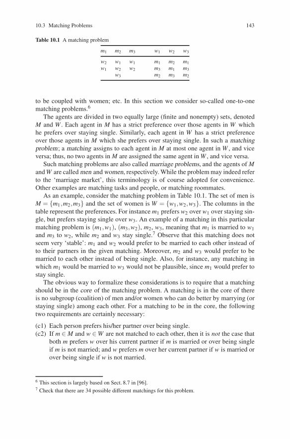
Table 10.1 A matching problem

m1 m2 m3 w1 w2 w3

w2 w1 w1 m1 m2 m1w1 w2 w2 m3 m1 m3

w3 m2 m3 m2

to be coupled with women; etc. In this section we consider so-called one-to-onematching problems.6

The agents are divided in two equally large (finite and nonempty) sets, denotedM and W . Each agent in M has a strict preference over those agents in W whichhe prefers over staying single. Similarly, each agent in W has a strict preferenceover those agents in M which she prefers over staying single. In such a matchingproblem; a matching assigns to each agent in M at most one agent in W , and viceversa; thus, no two agents in M are assigned the same agent in W , and vice versa.

Such matching problems are also called marriage problems, and the agents of Mand W are called men and women, respectively. While the problem may indeed referto the ‘marriage market’, this terminology is of course adopted for convenience.Other examples are matching tasks and people, or matching roommates.

As an example, consider the matching problem in Table 10.1. The set of men isM = {m1,m2,m3} and the set of women is W = {w1,w2,w3}. The columns in thetable represent the preferences. For instance m1 prefers w2 over w1 over staying sin-gle, but prefers staying single over w3. An example of a matching in this particularmatching problem is (m1,w1), (m3,w2), m2, w3, meaning that m1 is married to w1and m3 to w2, while m2 and w3 stay single.7 Observe that this matching does notseem very ‘stable’: m1 and w2 would prefer to be married to each other instead ofto their partners in the given matching. Moreover, m2 and w3 would prefer to bemarried to each other instead of being single. Also, for instance, any matching inwhich m1 would be married to w3 would not be plausible, since m1 would prefer tostay single.

The obvious way to formalize these considerations is to require that a matchingshould be in the core of the matching problem. A matching is in the core of thereis no subgroup (coalition) of men and/or women who can do better by marrying (orstaying single) among each other. For a matching to be in the core, the followingtwo requirements are certainly necessary:

(c1) Each person prefers his/her partner over being single.(c2) If m ∈ M and w ∈ W are not matched to each other, then it is not the case that

both m prefers w over his current partner if m is married or over being singleif m is not married; and w prefers m over her current partner if w is married orover being single if w is not married.

6 This section is largely based on Sect. 8.7 in [96].7 Check that there are 34 possible different matchings for this problem.


Obviously, if (c1) were violated then the person in question could improve bydivorcing and becoming single; if (c2) were violated then m and w would both bebetter off by marrying each other. A matching satisfying (c1) and (c2) is called sta-ble. Hence, any matching in the core must be stable. Interestingly, the converse isalso true: any stable matching is in the core. To see this, suppose there is a match-ing outside the core and satisfying (c1) and (c2). Then there is a coalition of agentseach of whom can improve by marrying or staying single within that coalition. Ifa member of the coalition improves by becoming single, then (c1) is violated. Iftwo coalition members improve by marrying each other, then (c2) is violated. Thiscontradiction establishes the claim that stable matchings must be in the core. Thus,the core of a matching problem is the set of all stable matchings.

How can stable matchings be computed? A convenient procedure is the deferredacceptance procedure proposed in [41]. In this procedure, the members of one of thetwo parties propose and the members of the other party accept or reject proposals.Suppose men propose. In the first round, each man proposes to his favorite woman(or stays single if he prefers that) and each woman, if proposed to at least once,chooses her favorite man among those who have proposed to her (which may meanstaying single). This way, a number of couples may form, and the involved menand women are called ‘engaged’. In the second round, the non-engaged men (inparticular, rejected men) propose to their second-best woman (or stay single); theneach woman again picks here favorite among the men who proposed to her includingpossibly the man to whom she is currently engaged. The procedure continues untilall proposals are accepted. Then all currently engaged couples marry and a matchingis established.

It is not hard to verify that this matching is stable. A man who stays single wasrejected by all women he preferred over staying single and therefore can find nowoman who prefers him over her husband or over being single. A woman who stayssingle was never proposed to by any man whom she prefers over staying single.Consider, finally, an m ∈ M and a w ∈ W who are married but not to each other. Ifm prefers w over his current wife, then w must have rejected him for a better partnersomewhere in the procedure. If w prefers m over her current husband, then m hasnever proposed to her and, thus, prefers his wife over her.

Of course, the deferred acceptance procedure can also be applied with women asproposers, resulting in a stable matching that is different in general.

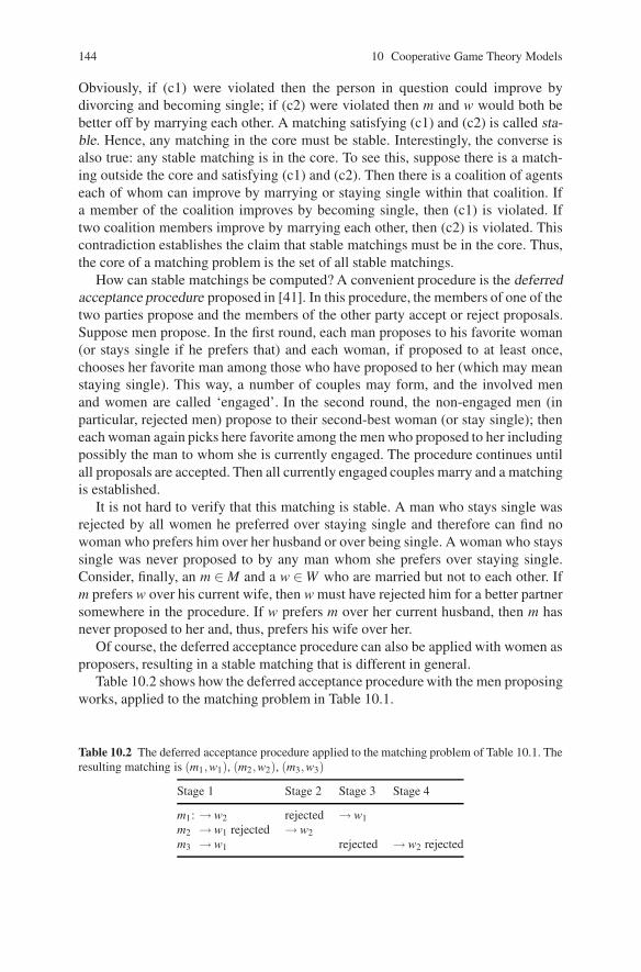
Table 10.2 shows how the deferred acceptance procedure with the men proposingworks, applied to the matching problem in Table 10.1.

Table 10.2 The deferred acceptance procedure applied to the matching problem of Table 10.1. Theresulting matching is (m1,w1), (m2,w2), (m3,w3)

Stage 1 Stage 2 Stage 3 Stage 4

m1: → w2 rejected → w1m2 → w1 rejected → w2m3 → w1 rejected → w2 rejected

10.4 House Exchange 145

There may be other stable matchings than those found by applying the deferredacceptance procedure with the men and with the women proposing. It can be shownthat the former procedure – with the men proposing – results in a stable matchingthat is optimal, among all stable matchings, from the point of view of the men,whereas the latter procedure – with the women proposing – produces the stablematching optimal from the point of view of the women. See also Problems 10.6and 10.7.

10.4 House Exchange

In a house exchange problem each one of finitely many agents owns a house, andhas a preference over all houses. The purpose of the exchange is to make the agentsbetter off. A house exchange problem is an exchange economy with as many goodsas there are agents, and where each agent is endowed with one unit of a different,indivisible good.8

Formally, the player set is N = {1, . . . ,n}, and each player i ∈ N owns house hi,and has a strict preference of the set of all (n) houses. In a core allocation, eachplayer obtains exactly one house, and there is no coalition that can make each ofits members strictly better off by exchanging their initially owned houses amongthemselves.

As an example, consider the house exchange problem in Table 10.3. In this prob-lem there are six possible different allocations of the houses. Table 10.4 lists theseallocations and also which coalition could improve by exchanging their own houses.

Table 10.3 A house exchange problem with three players. For instance, player 1 prefers the houseof player 3 over the house of player 2 over his own house

Player 1 Player 2 Player 3

h3 h1 h2h2 h2 h3h1 h3 h1

Table 10.4 Analysis of the house exchange problem of Table 10.3. There are two core allocations

Player 1 Player 2 Player 3 Improving coalition(s)

h1 h2 h3 {1,2}, {1,2,3}h1 h3 h2 {2}, {1,2}h2 h1 h3 None: core allocationh2 h3 h1 {2}, {3}, {2,3}, {1,2,3}h3 h1 h2 None: core allocationh3 h2 h1 {3}

8 This section is based largely on Sect. 8.5 in [96].


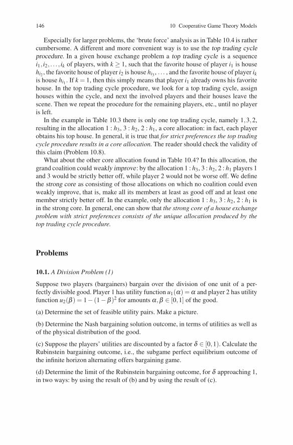
Especially for larger problems, the ‘brute force’ analysis as in Table 10.4 is rathercumbersome. A different and more convenient way is to use the top trading cycleprocedure. In a given house exchange problem a top trading cycle is a sequencei1, i2, . . . , ik of players, with k ≥ 1, such that the favorite house of player i1 is househi2 , the favorite house of player i2 is house hi3 , . . . , and the favorite house of player ikis house hi1 . If k = 1, then this simply means that player i1 already owns his favoritehouse. In the top trading cycle procedure, we look for a top trading cycle, assignhouses within the cycle, and next the involved players and their houses leave thescene. Then we repeat the procedure for the remaining players, etc., until no playeris left.

In the example in Table 10.3 there is only one top trading cycle, namely 1,3,2,resulting in the allocation 1 : h3, 3 : h2, 2 : h1, a core allocation: in fact, each playerobtains his top house. In general, it is true that for strict preferences the top tradingcycle procedure results in a core allocation. The reader should check the validity ofthis claim (Problem 10.8).

What about the other core allocation found in Table 10.4? In this allocation, thegrand coalition could weakly improve: by the allocation 1 : h3, 3 : h2, 2 : h1 players 1and 3 would be strictly better off, while player 2 would not be worse off. We definethe strong core as consisting of those allocations on which no coalition could evenweakly improve, that is, make all its members at least as good off and at least onemember strictly better off. In the example, only the allocation 1 : h3, 3 : h2, 2 : h1 isin the strong core. In general, one can show that the strong core of a house exchangeproblem with strict preferences consists of the unique allocation produced by thetop trading cycle procedure.

Problems

10.1. A Division Problem (1)

Suppose two players (bargainers) bargain over the division of one unit of a per-fectly divisible good. Player 1 has utility function u1(α) = α and player 2 has utilityfunction u2(β ) = 1− (1−β )2 for amounts α,β ∈ [0,1] of the good.

(a) Determine the set of feasible utility pairs. Make a picture.

(b) Determine the Nash bargaining solution outcome, in terms of utilities as well asof the physical distribution of the good.

(c) Suppose the players’ utilities are discounted by a factor δ ∈ [0,1). Calculate theRubinstein bargaining outcome, i.e., the subgame perfect equilibrium outcome ofthe infinite horizon alternating offers bargaining game.

(d) Determine the limit of the Rubinstein bargaining outcome, for δ approaching 1,in two ways: by using the result of (b) and by using the result of (c).

Problems 147


Suppose that two players (bargainers) bargain over the division of one unit of aperfectly divisible good. Assume that player 1 has utility function u(α) (0 ≤ α ≤ 1)and player 2 has utility function v(α) = 2u(α) (0 ≤ α ≤ 1).

Determine the physical distribution of the good according to the Nash bargainingsolution. Can you say something about the resulting utilities? (Hint: use the relevantproperties of the Nash bargaining solution.)


Suppose that two players (bargainers) bargain over the division of two units of aperfectly divisible good. Assume that player 1 has a utility function u(α) = α

2 (0 ≤α ≤ 2) and player 2 has utility function v(α) = 3

√α (0 ≤ α ≤ 2).

(a) Determine the physical distribution of the good according to the Rubinsteinbargaining procedure, for any discount factor 0 < δ < 1.

(b) Use the result to determine the Nash bargaining solution distribution.

(c) Suppose player 1’s utility function changes to w(α) = α for 0 ≤ α ≤ 1.6 andw(α) = 1.6 for 1.6≤ α ≤ 2. Determine the Nash bargaining solution outcome, bothin utilities and in physical distribution, for this new situation.

10.4. An Exchange Economy

Consider an exchange economy with two agents A and B and two goods. Theagents are endowed with initial bundles eA = (3,1) and eB = (1,3). Their prefer-ences are represented by the utility functions uA(x1,x2) = ln(x1 + 1)+ ln(x2 + 2)and uB(x1,x2) = 3ln(x1 + 1)+ ln(x2 + 1).

(a) Compute the demand functions of the agents.

(b) Compute Walrasian equilibrium prices and the equilibrium allocation.

(c) Compute the contract curve and the core. Sketch the Edgeworth box.

(d) Show that the Walrasian equilibrium allocation is in the core.

(e) How would you set up a two-person bargaining problem associated with thiseconomy? Would it make sense to consider the Nash bargaining solution in order tocompute an allocation? Why or why not?

10.5. The Matching Problem of Table 10.1 Continued9

(a) Apply the deferred acceptance procedure to the matching problem of Table 10.1with the women proposing.

(b) Are there any other stable matchings in this example?

9 Problems 10.5–10.7 are taken from [96].


Table 10.5 The matching problem of Problem 10.6

m1 m2 m3 w1 w2 w3

w1 w1 w1 m1 m1 m1w2 w2 w3 m2 m3 m2w3 w3 w2 m3 m2 m3

Table 10.6 The matching problem of Problem 10.7

m1 m2 m3 w1 w2 w3

w2 w1 w1 m1 m3 m1w1 w3 w2 m3 m1 m3w3 w2 w3 m2 m2 m2

10.6. Another Matching Problem

Consider the matching problem with three men, three women, and preferences as inTable 10.5.

(a) Compute the two matchings produced by the deferred acceptance procedure withthe men and with the women proposing.

(b) Are there any other stable matchings?

(c) Verify the claim made in the text about the optimality of the matchings in (a) forthe men and the women, respectively.

10.7. Yet Another Matching Problem: Strategic Behavior

Consider the matching problem with three men, three women, and preferences as inTable 10.6.

(a) Compute the two matchings produced by the deferred acceptance procedure withthe men and with the women proposing.

(b) Are there any other stable matchings?

Now consider the following noncooperative game. The players are w1, w2, and w3.The strategy set of a player is simply the set of all possible preferences over the men.(Thus, each player has 16 different strategies.) The outcomes of the game are thematchings produced by the deferred acceptance procedure with the men proposing,assuming that each man uses his true preference given in Table 10.6.

(c) Show that the following preferences form a Nash equilibrium: w2 and w3 usetheir true preferences, as given in Table 10.6; w1 uses the preference (m1,m2,m3).Conclude that sometimes it may pay off to lie about one’s true preference. (Hint: ina Nash equilibrium, no player can gain by deviating.)

10.8. Core Property of Top Trading Cycle Procedure

Show that for strict preferences the top trading cycle results in a core allocation.

Problems 149

Table 10.7 The house exchange problem of Problem 10.10

Player 1 Player 2 Player 3 Player 4

h3 h4 h1 h3h2 h1 h4 h2h4 h2 h3 h1h1 h3 h2 h4

10.9. House Exchange with Identical Preferences

Consider the n-player house exchange problem where all players have identicalstrict preferences. Find the house allocation(s) in the core.

10.10. A House Exchange Problem10

Consider the house exchange problem with four players in Table 10.7.Compute all core allocations and all strong core allocations.

10.11. Cooperative Oligopoly

Consider the Cournot oligopoly game with n firms with different costs c1,c2, . . . ,cn.(This is the game of Problem 6.2 with heterogenous costs.) As before, each firmi offers qi ≥ 0, and the price-demand function is p = max{0,a−∑n

i=1 qi}, where0 < ci < a for all i.

(a) Show that the reaction function of player i is

qi = max{0,a− ci−∑ j =i qi

2}.

(b) Show that the unique Nash equilibrium of the game is q∗ = (q∗1, . . . ,q∗n) with

q∗i =a−nci + ∑ j =i c j

n + 1,

for each i, assuming that this quantity is positive.

(c) Derive that the corresponding profits are

(a−nci + ∑ j =i c j)2

(n + 1)2

for each player i.

Let the firms now be the players in a cooperative TU-game with player set N ={1,2, . . . ,n}, and consider a coalition S ⊆ N. What is the total profit that S can makeon its own? This depends on the assumptions that we make on the behavior of the

10 Taken from [83].


players outside S. Very pessimistically, one could solve the problem

maxqi:i∈S

minq j : j/∈S

∑i∈S

Pi(q1, . . . ,qn),

which is the profit that S can guarantee independent of the players outside S. Thisview is very pessimistic because it presumes maximal resistance of the outside play-ers, even if this means that these outside players hurt themselves. In the present caseit is not hard to see that this results in zero profit for S.

Two alternative scenarios are: S plays a Cournot–Nash equilibrium in the (n−|S|+1)-player oligopoly game against the outside firms as separate firms, or S playsa Cournot–Nash equilibrium in the duopoly game against N \S.

In the first case we in fact have an oligopoly game with costs c j for every playerj /∈ S and with cost cS := min{ci : i ∈ S} for ‘player’ (coalition) S.

(d) By using the results of (a)–(c) show that coalition S obtains a profit of

v1(S) =[a− (n−|S|+ 1)cS+ ∑ j/∈S c j]2

(n−|S|+ 2)2

in this scenario. Thus, this scenario results in a cooperative TU-game (N,v1).

(e) Assume n = 3, a = 7, and ci = i for i = 1,2,3. Compute the core, the Shapleyvalue, and the nucleolus for the TU-game (N,v1).

(f) Show that in the second scenario, coalition S obtains a profit of

v2(S) =(a− 2cS + cN−S)2

9,

resulting in a cooperative game (N,v2).

(g) Assume n = 3, a = 7, and ci = i for i = 1,2,3. Compute the core, the Shapleyvalue, and the nucleolus for the TU-game (N,v2).

Documents

Game Theory || Cooperative Game Theory Models