Embed Size (px)
Citation preview

Gait analysis of paediatric patients with hemiparesis Page 1
Treball de Fi de Grau
Enginyeria en Tecnologies Industrials
Gait analysis of paediatric patients with hemiparesis
MEMÒRIA
Autor: Anna Muñoz Farré
Director: Josep Maria Font Llagunes
Convocatòria: Juny 2016

Gait analysis of paediatric patients with hemiparesis Page 2
Abstract
The main objective of this Final Project for the Bachelor Degree in Industrial Technology
Engineering is to study how the feedback device Walking o’Clock modifies gait pattern of
paediatric patients with hemiparesis. The project has been developed in collaboration with
personnel of Sant Joan de Déu Hospital (HSJD), that selected the three patients involved in
the study. The gait of these patients was captured in the UPC Biomechanics Laboratory, and
the kinematic analysis was performed using OpenSim, a free software tool developed by
Stanford University that is widely used by the scientific community.
Walking o’Clock, by Draco Systems, is an electronic device with an inertial measurement unit
(IMU). It was used to measure thigh orientation in the study, aided by the engineer who
created this product. By measuring this orientation, the physiotherapist would choose what
kind of feedback the patient should be put under to.
The patients’ movement was analysed under three different situations: natural gait, gait using
the device (with the feedback chosen) and gait after using the device (after feedback). Four
angular coordinates in the sagittal plane (hip flexion, pelvic tilt, knee flexion and ankle
dorsiflexion) were analysed and compared.
From the results, it was shown that the device modifies the gait pattern. However, depending
on the patient and the feedback, the walking kinematics was modified in different ways. In
some aspects, an improvement was found for the selected paediatric patients.
This report describes all the processes involved in the analysis, as well as the methodology
used. To obtain the motion data, the human body has been modelled as a multibody system
with rigid bodies and ideal joints with different degrees of freedom. The process to export the
kinematics data using OpenSim is explained in detail. From the position of each body,
inverse kinematics determines the configuration (position and orientation) of the multibody
system along time.

Gait analysis of paediatric patients with hemiparesis Page 3

Gait analysis of paediatric patients with hemiparesis Page 4
Contents ABSTRACT ___________________________________________________ 2
CONTENTS ___________________________________________________ 4
1. GLOSSARY ______________________________________________ 7
2. INTRODUCTION ___________________________________________ 82.1. Origin of the project and motivation ................................................................ 8
2.2. Introduction to Biomechanics .......................................................................... 8
2.3. Objectives of the project ................................................................................ 11
2.4. Project Scope ................................................................................................ 11
3. BACKGROUND __________________________________________ 123.1. Biomechanics of human gait ......................................................................... 12
3.1.1. Reference planes ................................................................................................ 123.1.2. Gait cycle ............................................................................................................ 123.1.3. Gait analysis ........................................................................................................ 15
3.2. Cerebral palsy ............................................................................................... 163.2.1. Children with cerebral palsy ................................................................................ 163.2.2. Gait analysis in hemiparesis ............................................................................... 17
3.3. The patients ................................................................................................... 18
4. WALKING O’CLOCK DEVICE _______________________________ 204.1. Description ..................................................................................................... 20
4.2. Functioning .................................................................................................... 20
5. MUSCULOSKELETAL MODEL ______________________________ 225.1. Parameters of the musculoskeletal model .................................................... 22
5.2. Model used in the project .............................................................................. 235.2.1. Bodies ................................................................................................................. 235.2.2. Joints ................................................................................................................... 245.2.3. Generalized coordinates ..................................................................................... 25
5.3. Marker protocol .............................................................................................. 265.3.1. The design of the protocol .................................................................................. 265.3.2. Protocol used in the project ................................................................................ 27
6. MOTION CAPTURE _______________________________________ 286.1. The Biomechanics Laboratory ...................................................................... 28
6.1.1. Laboratory equipment ......................................................................................... 286.1.2. Calibration ........................................................................................................... 29

Gait analysis of paediatric patients with hemiparesis Page 5
6.2. Procedure for motion capture ........................................................................ 31
6.3. Motion capture and data export .................................................................... 326.3.1. Placement of the markers ................................................................................... 326.3.2. Optical tracking ................................................................................................... 336.3.3. The walking path ................................................................................................. 336.3.4. Write the TRC file ................................................................................................ 34
7. KINEMATICS ANALYSIS ___________________________________ 357.1. Introduction to OpenSim ................................................................................ 35
7.2. Scaling the model .......................................................................................... 36
7.3. Inverse kinematics ......................................................................................... 407.3.1. Calculation of inverse kinematics ....................................................................... 407.3.2. Solution with OpenSim ....................................................................................... 40
8. RESULTS AND DISCUSSION _______________________________ 428.1. Methodology .................................................................................................. 42
8.2. Maria .............................................................................................................. 468.2.1. Hip flexion ........................................................................................................... 468.2.2. Pelvic tilt .............................................................................................................. 488.2.3. Knee flexion ........................................................................................................ 498.2.4. Ankle dorsiflexion ................................................................................................ 51
8.3. Jordi ............................................................................................................... 548.3.1. Hip flexion ........................................................................................................... 548.3.2. Pelvic tilt .............................................................................................................. 568.3.3. Knee flexion ........................................................................................................ 578.3.4. Ankle dorsiflexion ................................................................................................ 59
8.4. Isabel ............................................................................................................. 628.4.1. Hip flexion ........................................................................................................... 628.4.2. Pelvic tilt .............................................................................................................. 648.4.3. Knee flexion ........................................................................................................ 658.4.4. Ankle dorsiflexion ................................................................................................ 67
9. CONCLUSIONS __________________________________________ 70
10. ACKNOWLEDGEMENTS ___________________________________ 72
11. REFERENCES ___________________________________________ 73


Gait analysis of paediatric patients with hemiparesis Page 7
1. Glossary
There are some terms that are used with their acronyms in the project. Note that they will be
defined later on the project. The list is presented here:
• GC:GaitCycle• IC:InitialContact• IK:Inversekinematics• DOF:Degreeoffreedom• N:Natural• F:Feedback• F1:Feedback1• F2:Feedback2• A:AfterFeedback• ROM:RangeofMotion• RMSE:RootMeanSquareError

Gait analysis of paediatric patients with hemiparesis Page 8
2. Introduction
This Final Project for the Bachelor’s degree in Industrial Technology Engineering is entitled “Gait
analysis of paediatric patients with hemiparesis”, and is part of the line work of the
Biomechanical Engineering Group (BIOMEC) of the Department of Mechanical Engineering at
the Barcelona School of Industrial Engineering, at Universitat Politècnica de Catalunya
(ETSEIB, UPC).
This project has been developed in collaboration with Sant Joan de Déu Hospital (HSJD),
specifically with the Research Team, that has provided with the patients involved in the study,
and with Draco Systems, the engineering company that has designed the device used in the
study. The results and conclusions of this project will be used by the HSJD for further
investigations.
2.1. Origin of the project and motivation
First of all, the author of this project wanted to do a project related to biomechanics and, if
possible, with some kind of contribution to a research area, since she will be coursing the
Master in Industrial Engineering with the speciality in Biomedicine.
Second, the Research Centre of HSJD does not have a biomechanics laboratory on their
facilities. Therefore, months ago, they approached the Biomechanical Engineering Group of the
UPC to see if they could have any kind of collaboration in the future.
At the same time, an engineering company, Draco Systems, had designed a prototype of a
device (named Walking o’Clock), under the demands of the HSJD, which would assist and
modify the gait pattern of paediatric patients with a walking disability. However, it had not been
quantitatively assessed yet.
After a couple of meetings between the HSJD team and the BIOMEC team, the idea of the
project was decided. It would be a pilot study on how this device modified the gait pattern of
paediatric patients with hemiparesis, who would be selected by the clinical staff of HSJD. Using
the equipment in the Biomechanics Laboratory in the university (ETSEIB), captures of gait
would be taken. Then, the measurements would be analysed with the software OpenSim and
the results would be compared to those of a healthy gait.
2.2. Introduction to Biomechanics
Biomechanics is the study of the structure and function of biological systems such
as humans, animals, plants, organs, fungi, and cells by means of the methods of mechanics [1].
In this project, the kinematics of human gait will be analysed. Due to the complexity of human

Gait analysis of paediatric patients with hemiparesis Page 9
body, formed by multiple systems and tissues, some simplifications are made to analyse
movement. The human skeleton is in charge of the movement from joints between bones,
which is possible thanks to the muscles, which coordinate their action from the orders generated
by the central nervous system.
Musculoskeletal models are effective for visualizing human movement, analysing the functional
capacity of muscles, and designing improved surgical procedures [2]. They model the human
body as a system formed by several solids or rigid segments, joined together through joints that
allow different degrees of freedom. This includes the study of the kinematic and dynamic motion
of human body in the field of rigid body mechanics.
The goal of this project is to carry out a pilot study on how a device modifies the gait pattern.
This device, named Walking o’Clock, is still a prototype, whose operation will be explained in
detail further in this work. Three patients, selected by the clinical staff of Hospital Sant Joan de
Déu, will be analysed independently. Simultaneously, their gait patterns will be compared to the
standard one [3]. Their gait pattern will be analysed from motion captures taken in the
Biomechanics Laboratory of the Thechnical University of Catalonia, UPC, in ETSEIB. After
processing the data from the captures, the kinematic analysis is done through the free software
OpenSim [2], developed by the National Center for Simulation in Rehabilitation Research of the
Stanford University (California, USA).
Child patients with hemiparesis attend physiotherapy, as often as their pathology demands.
However, it is never as much as they need. This means that, after assisting therapy, the aspects
that they have worked improve for a few days, but tend to go back to their original state if
therapy is not repeated soon enough. The impossibility of having a training with a
physiotherapist every day, as they would need, complicates and slows the healing process.
Therefore, if patients could have something that complemented the therapy, the process would
be improved. This is where the device makes sense. Since it would be affordable, it would allow
patients to have a daily assistant. They could use it every day, whenever and wherever they
wanted. Of course, the use of the device would be controlled and supervised by their
physiotherapist.


Gait analysis of paediatric patients with hemiparesis Page 11
2.3. Objectives of the project
The general goal has been defined, in accordance with the HSJD team and the UPC
Biomechanics group, as the study of how a device modifies a gait pattern in three paediatric
patients with hemiparesis. These general goal is developed into these specific objectives:
• Analysing the gait of three paediatric patients with hemiparesis in three different
situations, using the UPC Biomechanics Laboratory, and investigating how the Walking
O’Clock device modifies the gait pattern of each patient.
• Finding a model and a protocol to reproduce the motion as close to reality as possible.
• Obtaining kinematic variables of the gait using the OpenSim software.
• Comparing the results of the three different situations for each patient, and comparing
them to the standard healthy gait to quantify the change achieved by using the device.
• Reporting the results obtained to the Research Team of HSJD.
2.4. Project Scope
The aim of this pilot study is to analyse how the device modifies the gait pattern of three children
patients with hemiparesis. Anyhow, it is important to keep in mind the timing and circumstances
of the study. First of all, each patient will have used the device for a short time, so they will not
have been able to adapt to its functioning as well as they would have been in case of having
used it for a longer time. Secondly, due to the fact that the device is a prototype, it has some
flaws and it might not be completely reliable. Moreover, the physiotherapist involved with the
project is still getting used to the device. However, the motion captures that will be taken will
show how the gait pattern of each patient changes after using it, so this changes will be
analysed with a more accurate and reliable method. Therefore, even if the device has some
error, it will not affect the analysis of the consequences of using it.
Then, the main goal of this project is to show how the use of this device would modify the gait
pattern of a patient and to see if the changes improve the gait. It is then a pilot study for what
could be a deeper study with more patients and longer time.

Gait analysis of paediatric patients with hemiparesis Page 12
3. Background
3.1. Biomechanics of human gait
3.1.1. Reference planes
The motion of limbs is described using three reference planes, which can be seen in Fig. 1 The
three reference planes of the anatomical position. The sagittal plane is any plane which divides
the part of the body into right and left portions; the median plane is the midline sagittal plane,
which divides the whole body into right and left halves. The frontal plane divides a body part into
front and back (anterior and posterior) portions. Finally, the transverse plane divides a body part
into upper and lower portions [4]. In this project, only the motion patterns in the sagittal plane will
be analysed.
Fig. 1 The three reference planes of the anatomical position [5]
3.1.2. Gait cycle
Human gait is the result of the complex interaction of several subsystems, the neuromuscular,
musculotendinous and osteoarticular, that generate together the necessary body dynamics for
bipedal movement. Walking uses a repetitious sequence of limb motions to simultaneously
move the body forward while also maintaining stance stability. As the body moves forward, one
limb serves as a mobile source of support while the other limb advances itself to a new support
site. For the transfer of body weight from one limb to the other, both feet are in contact with the
ground. A single sequence of these functions by one limb is called a gait cycle (GC).
Each GC is divided into the stance period, during which the foot is on the ground, which begins
with an initial contact (IC), and the swing period, when the foot is in the air for limb

Gait analysis of paediatric patients with hemiparesis Page 13
advancement, which begins as the toe is lifted from the floor (toe off). The GC begins with initial
double stance (bilateral foot contact with the floor), followed by the single limb support as the
opposite foot is lifted for swing (single stance, SLS). The duration of such phase is the best
index of the limb’s support capability, with longer relative durations reflecting greater stability.
The third subdivision is the terminal double limb stance, which begins with floor contact by the
other foot and continues until the original stance limb is lifted for swing.
The generic normal distribution of the floor contact periods approximates 60% for stance and
40% for swing, which varies with the person’s walking velocity [4]. It shows an inverse
relationship to walking speed, so the change in stance and swing times becomes progressively
greater as the speed slows. An opposite relationship can be found among the subdivisions of
stance, as walking faster proportionally lengthens single stance and shortens the two double
stance intervals. The subdivisions in gait are shown in Fig. 2.
Fig. 2 . Subdivisions of gait and their relationships to the pattern of bilateral floor contact (Adapted
from [6])
Since one action flows into the next, there is no specific starting or ending point. At the
Biomechanics Laboratory in the university, measures of complete GC for each limb can be
taken. Taking into account that normal people initiate floor contact with their heel, as the right
feet is the first one to step on the pressure plate, its captures cycle will be from heel strike to
heel strike (HE-HE). On the other hand, the captured cycle for the left limb will start a few
instants later, going from toe off to toe off (TO-TO).
The GC has also been identified by the descriptive term stride, which is the period from initial
contact to initial contact of the same limb, which comprises two steps. The step is the distance
between initial swing and initial contact of the same limb. The relationship between step and
stride is seen in Fig. 3.
Gait analysis of paediatric patients with hemiparesis Page 14
Fig. 3 Step versus stride (Adapted from [6])
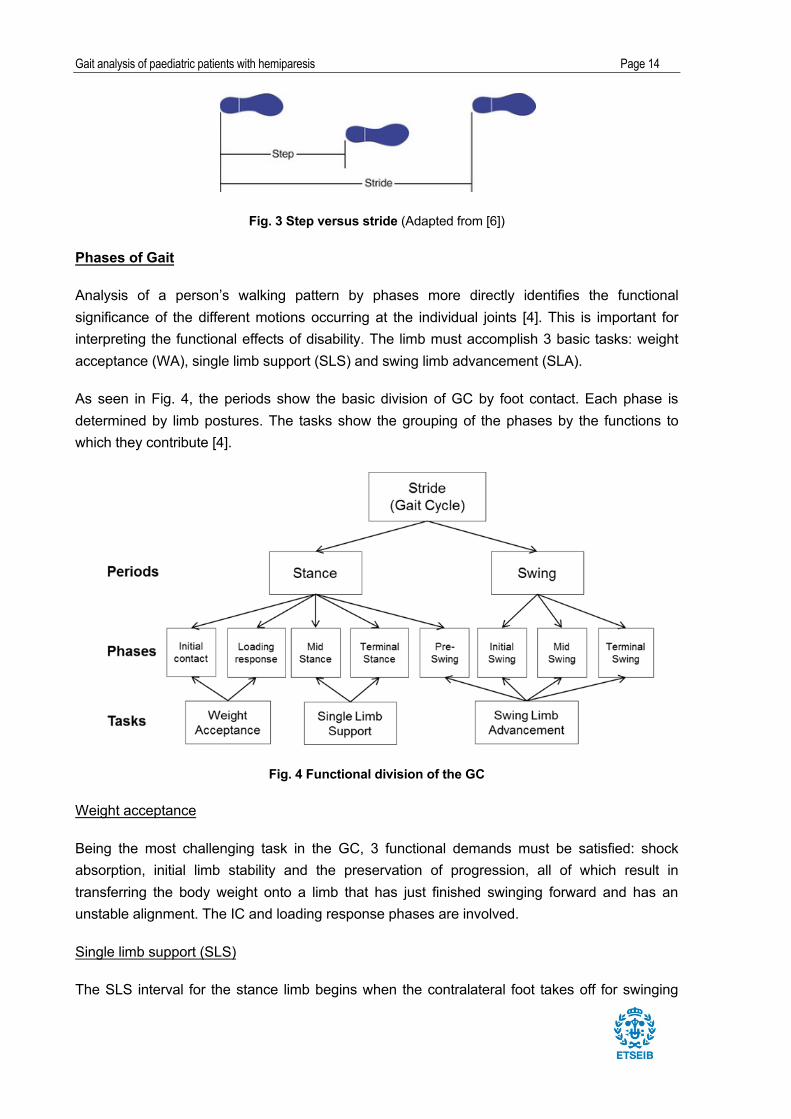
Phases of Gait
Analysis of a person’s walking pattern by phases more directly identifies the functional
significance of the different motions occurring at the individual joints [4]. This is important for
interpreting the functional effects of disability. The limb must accomplish 3 basic tasks: weight
acceptance (WA), single limb support (SLS) and swing limb advancement (SLA).
As seen in Fig. 4, the periods show the basic division of GC by foot contact. Each phase is
determined by limb postures. The tasks show the grouping of the phases by the functions to
which they contribute [4].
Fig. 4 Functional division of the GC
Weight acceptance
Being the most challenging task in the GC, 3 functional demands must be satisfied: shock
absorption, initial limb stability and the preservation of progression, all of which result in
transferring the body weight onto a limb that has just finished swinging forward and has an
unstable alignment. The IC and loading response phases are involved.
Single limb support (SLS)
The SLS interval for the stance limb begins when the contralateral foot takes off for swinging

Gait analysis of paediatric patients with hemiparesis Page 15
and continues until the opposite foot again contacts the ground. In this case, the one limb has
the total responsibility of supporting the body weight in both the sagittal and coronal planes
while progression continues. Mid stance and terminal stance are involved in SLS.
Swing limb advancement
Preparatory posturing begins in stance in order to meet the high demands of advancing the
limb. Then, the limb swings through 3 postures as it lifts itself, advances to complete the stride
length and prepares for the next stance interval. Four gait phases are involved: pre-swing (end
of stance), initial swing, mid swing and terminal swing.
Determinants of gait (motion patterns)
Fig. 5 shows sagittal plane joint angles (in degrees) during a single gait cycle of pelvic tilt, right
hip (flexion positive), knee (flexion positive) and ankle (dorsiflexion positive).
Fig. 5 Sagittal plane joint angles during a single gait cycle of pelvic tilt and right hip, knee and ankle [7].
3.1.3. Gait analysis
Gait analysis is used for two very different purposes: to aid directly in the treatment of individual
patients and to improve our understanding of gait, through research. No single method of
analysis is suitable for such a wide range of uses and a number of different methodologies have

Gait analysis of paediatric patients with hemiparesis Page 16
been developed [4].
Basically, there are 5 measurement systems. Three of these focus on the specific events that
constitute the act of walking. Motion analysis defines the magnitude and timing of individual joint
movements. Dynamic electromyography identifies the period and relative intensity of muscle
function. Force plate recordings display the functional demands being experienced during the
weight-bearing period. Each system serves as a diagnostic technique for one facet of gait. The
2 remaining gait analysis techniques summarize the effects of the person’s gait mechanics. One
measures the patient’s stride characteristics to determine overall walking capability, while
efficiency is revealed by energy cost measurements. There are several choices of technique
within each of these 5 basis measurements systems, which differ in cost, convenience and
completeness of the data provided. As there is not a single optimal system, selections are
based on the needs, staffing, and finances of the research situation [8].
3.2. Cerebral palsy
Cerebral palsy is defined as a group of permanent disorders in the development of movement
and posture causing activity limitations that are attributed to non-progressive disturbances that
occurred in the developing foetal or infant brain [3]. Along with the motor disorders, disturbances
of sensation, perception, cognition, communication and behaviour can appear, as well as
epilepsy or secondary musculoskeletal problems. Not only affects it the cortical brain, but all of
the brain’s functions as well. In the case of gait, it influences the musculoskeletal system
function.
The characteristics of cerebral palsy were given by Gage [3] as follows:
1. Loss of selective muscle control
2. Dependence on primitive reflex patterns for ambulation
3. Abnormal muscle tone
4. Relative imbalance between muscle agonists and antagonists across joints
5. Deficient equilibrium reactions
It is important to keep in mind that the way cerebral palsy affects the joint rotation varies
considerably between one patient and another.
3.2.1. Children with cerebral palsy
Spasticity refers to stiff or rigid muscles, an overactive response of a muscle to rapid stretching.
It can also be called unusual stress or increased muscle tone. Reflexes are stronger or
exaggerated. This condition can interfere with the activity of walking, movement or speech [9].
Even if children with cerebral palsy do not have severe spasticity or weakness, they usually

Gait analysis of paediatric patients with hemiparesis Page 17
have problems with motor control, including difficulty in moving their limbs. Moreover, balance is
a significant problem in most children. The aetiology of this abnormality is not clear, but it is
probably secondary to poor connections between the cerebellum and most of the other higher
centres of the brain, as well as connections to descending neurons to the spinal cord.
Paediatric hemiparesis
Paediatric spastic hemiparesis is a mild form of cerebral palsy in children, which affects only half
of the body. It is a neurologic condition which complicates movement in that part of the body,
but without reaching paralysis. Therefore, it is a minor degree of hemiplegia, which is total
paralysis and affects only one out of thousand born children [10].
The most typical manifestation consists on abnormal postures and limb deformities due to
weakness of some muscles and spasticity of others. In the upper limb this results in a difficulty
in performing manual activities; the typical stance is with an elbow, wrist and fingers flexion. At
the bottom, movement (gait) problems can be found, being the typical stance with flexed knee
and ankle [11].
Hemiparetic gait patterns
In the case of hemiparesis, the usual gait pattern is when the patient walks slowly, resting their
weight on the unaffected limb, moving the paretic limb in arc, while the affected arm remains
attached to the body in semi-flexion [1]. The affected lower limb acts as if it were longer, being
extended. Moreover, the ankle is internally rotated in clubfoot attitude (equinovarus), so all
propulsion movement focuses on the hip. Thus, the hip and knee will be stiff and slightly flexed.
As a result, the foot describes an arc foot internal concavity to go forward, touching the ground
with the tip and the anterolateral face, tending to drag along the floor. The strong gluteal and
quadriceps muscle groups are generally spastic and the most affected muscles are the
iliopsoas (the strongest of the hip flexors), the hamstrings and the dorsiflexors of the foot.
Moreover, almost always the posterior ones are better preserved than the anterior ones.
3.2.2. Gait analysis in hemiparesis
Hemiparesis is a common pathology in children. Therefore, there are several studies on the
subject. For the professionals involved with patients with hemiparesis, observational gait
analysis, linked with a thorough clinical evaluation, provides a tool for documenting gait
deviations and can be used to determine causes of walking challenges. Physiotherapists use it
on their daily basis. There are several predefined and implemented forms and codes for defining
the degree of the pathology.
In the case of hemiparesis, there is a wide range of studies. Both observational and
instrumented three-dimensional motion analyses are used to identify abnormal movement
patterns during gait and underlying causes of deviations. Gait analysis provides an objective
record of a child’s gait before and after therapeutic intervention and should be considered a vital

Gait analysis of paediatric patients with hemiparesis Page 18
part of the clinician’s decision making [8].
During walking, the centre of body mass must pass from behind the weight bearing foot to in
front of it. For this to take place, the foot must function as a sagittal plane pivot. Because the
range required for this motion is approximately five times as great as both frontal and transverse
plane motion, its evaluation becomes an essential part of a biomechanical assessment [12].
Gait abnormalities in children with cerebral palsy can affect movement at the hip, knee, and
ankle. Therefore, a wide range of studies on hemiparesis focus on the parameters hip flexion,
knee flexion, pelvic tilt, and ankle dorsiflexion of the sagittal plane. By looking at the patterns of
this parameters, specific gait problems can be distinguished, due to deviations. For example,
stiff-knee gait can be distinguished with the knee angle pattern. It is seen as an excessive knee
flexion in stance continued into swing and a delayed and decreased knee flexion during swing.
For the purpose of this study and given the available facilities, the technique used for this study
will be motion capture. Even though it gives three-dimensional information, only motion in
sagittal plane will be studied.
3.3. The patients
Three patients with hemiparesis from Hospital Sant Joan de Déu were analysed at the
Biomechanics Laboratory. The physiotherapist made a quick exploration on the patients, before
proceeding with the movement captures. The relevant patient information for this project is listed
in Table 1(their real names have been changed):
Number Patient Age Weight (kg) Pathology Notes
1 Maria 14 50,2 Right spastic hemiparesis -
2 Jordi 15 55,0 Right spastic hemiparesis He wears a Foot-Up
3 Isabel 11 61,8 Right spastic hemiparesis She wears a DAFO
Table 1 Patient information
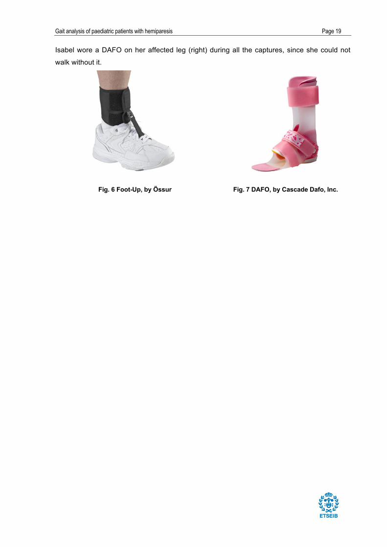
A Foot-Up (Fig. 6) is a lightweight ankle-foot orthosis by Össur that offers dynamic support
for drop foot or similar complaints for which support of dorsiflexion is desirable. Note that
Jordi did not wear the Foot-Up during the motion captures. Therefore, it did not affect the
study.
A Dynamic Ankle-Foot Orthosis (DAFO) (Fig.7), by Cascade Dafo, Inc, is a brand name for a
thin, flexible contoured brace, wrapping around the foot, which improves stability. Note that
Gait analysis of paediatric patients with hemiparesis Page 19
Isabel wore a DAFO on her affected leg (right) during all the captures, since she could not
walk without it.
Fig. 6 Foot-Up, by Össur Fig. 7 DAFO, by Cascade Dafo, Inc.

Gait analysis of paediatric patients with hemiparesis Page 20
4. Walking o’Clock device
4.1. Description
The walking o’Clock device is an electronic device with an inertial measurement unit (IMU) of
nine axes (triple-axis accelerometers, gyroscopes and magnetometers). It works using
quaternions to define the orientation of rigid bodies in three-dimensional space. It can record up
to 200 measurements per second.
4.2. Functioning
Only the functioning of what was used in the project will be explained. Following the
physiotherapist instructions, the device was placed on both tights of the patients with a Velcro
strap. Therefore, it was measuring the angle of the thigh with respect to the vertical axis in the
sagittal plane. Since trunk orientation is vertical and almost constant during gait, it was
considered that the device gave a relatively accurate estimation of the patients’ hip flexion. Fig.
8 shows the device on the leg of patient Maria.
Fig. 8 On the left, the device on the leg of patient Maria. On the right, the device
First, with the patient standing straight, the device was set to angle 0° with the vertical axis to
the ground. During the capture, via Wi-Fi, it would analyse the angles from the vertical axis and
show their plot on screen. Then, as the capture stopped, it calculated the maximum and
minimum angle. With that information, the physiotherapist decided what the best feedback could
be.
The feedback can be sent through three ways: vibration, led or sound. Since some of the
patients presented disturbances of sensitivity, the vibration was found as unreliable. Then, using
earphones, the patient could hear the feedback.

Gait analysis of paediatric patients with hemiparesis Page 21
The way the feedback works is the following. A threshold angle is chosen, which can be either
of flexion or extension. Then, it can give feedback when the angle is under or when it is above
the chosen one. To explain it, a reference Fig.9 has been made. If the chosen angle is θ0, there
are two possible intervals: from 0° to θ0 (called interval 1) and above θ0 (interval 2). Thus,
depending on the interval chosen, the patient will hear a sound either when they are under or
above the angle θ. Taking the case of flexion, if the intention is for the patient to increase the
angle, the feedback will be set on interval 1 and they will be told to keep flexing until the sound
stops. On the other hand, if they need to decrease it, the feedback will be set on interval 2 and
they will be told to stop flexing when they hear the sound. In the extension case, the angles will
be negative, but the methodology would be the same one.
The feedback chosen for each patient during the capture motion is detailed in section 7.
Fig. 9 Reference angle θ0 to explain the functioning of the feedback in the case of flexion
0°
!"
i1 i2

Gait analysis of paediatric patients with hemiparesis Page 22
5. Musculoskeletal model
5.1. Parameters of the musculoskeletal model
The study of human motion is based on the rigid body dynamics. The human body is defined as
a multibody system, where each body segment, which is made of bone and soft tissues, is then
assumed to be rigid. Thus, the inertial properties of each body can be defined through its mass,
position of centre of mass and tensor of inertia. Depending on the intended application of the
model, the complexity of it will vary. For example, simple non-muscle based models possess
few variables, but they do not allow the study of muscle coordination during motion.
The system includes joint models that define kinematical constraints among the bodies and
actuators that control them. These internal joints are modelled as rotations of one or more
degrees of freedom. Moreover, the external joints must be defined, such as the contact of the
feet with the ground. If there is not a fixed body, it is usual to consider that one of the system
bodies is linked to the reference frame with a joint that allows the six degrees of freedom (three
for rotation and three for translation). In this project, the pelvis will be linked to the ground (which
defines the reference frame).
The number of bodies does not usually match the number of bones in a human body. In the
case of a group of bodies that have a little relative movement among them, they may as well be
considered as one body. In this project, since gait will be analysed, the head arms and trunk
(HAT) are not considered in order to simplify the model. This practise is common when
analysing the lower limbs during walking.
There are different options to model the joints. The first one is to try to get as close to reality as
possible, by defining joints that only allow the rotations of human joints. This gives information
about joint forces between bodies (the movements not allowed by the articulations are
prevented by the called joint forces in classical mechanics). However, in biomechanics and
specifically in motion capture, which are not exact and which throw unavoidable errors, this kind
of forces could give resulting values that are far from reality.
There is the opposite option, which is to give more freedom to joints, by considering them as
spherical joints and allowing small capture errors that will cause movements not allowed in
reality. However, they would not be far from reality, since they would be the result of a real
motion capture. This option also simplifies the difficulty when it comes to calculations.
The description of the configuration of the multibody system is done through the definition of a
group of generalized coordinates associated to angles, and relative positions among the bodies.
In this case, the generalized coordinates are the allowed joint rotations. Even though they will
not be used in this project, the generalized velocities would be defined as time derivatives of the

Gait analysis of paediatric patients with hemiparesis Page 23
generalized coordinates.
Regarding forces and moments, the actuators can be defined by directly linking them to all the
generalized coordinates, so that each of the degrees of freedom is controlled by an actuator. In
the case of human body modelling, as many angular actuators as relative rotations between
bodies can be defined. For the ground joint, six actuators are defined (three linear and three
angular), which are important for the analysis.
Being the system holonomic (the number of independent coordinates is the same as the
number of degrees of freedom) and given the fact that its state is defined by a minimum number
of generalized coordinates, the motion equations can be defined with Lagrange ordinary
equations, as does the software OpenSim.
5.2. Model used in the project
The model used in the project is the Gait2392, provided by OpenSim. The model was created
by Darryl Thelen (University of Wisconsin-Madison); and Ajay Seth, Frank C. Anderson and
Scott L. Delp (Stanford University). Since the interest of the study was the lower body, the torso
was removed from the model, along with its degrees of freedom. Moreover, the metatarsal joints
of the model have been locked. This is due to the fact that they are not relevant to this study,
and the patients may wear shoes, thus the information of the captures with the markers will not
be enough to analyse the metatarsal joint.
The model that has been used for all the gait captures, even though it has been slightly modified
when needed is the one explained below.
5.2.1. Bodies
The model is formed by 11 bodies and ground. To define each of the bodies, their mass, the
position of its centre of inertia and the values of the elements of its central inertia tensor must be
specified. The different bodies of the model are listed in Table 2 and shown in Fig. 10:

Gait analysis of paediatric patients with hemiparesis Page 24
5.2.2. Joints
The system has a total of 18 degrees of freedom (DOF), 6 for the pelvis motion with respect to
the ground and the other 14 correspond to relative movements between the various bodies that
form the model. However, as mentioned, the 2 degrees of freedom of the metatarsal joints are
locked, thus the degrees of freedom disappear. Table 3 shows the existing joints, as well as the
number of degrees of freedom allowed for each joint.
Name of the body Name in
OpenSim
Ground ground
Pelvis pelvis
Left femur femur_l
Right femur femur_r
Left tibia tibia_l
Right tibia tibia_r
Left talus talus_l
Right talus talus_r
Left calcaneus calcn_l
Right calcaneus calcn_r
Left phalanx bone toes_l
Right phalanx bone toes_r
Table 2 Bodies of the multibody model
Fig. 10 Bodies of the model
Gait analysis of paediatric patients with hemiparesis Page 25
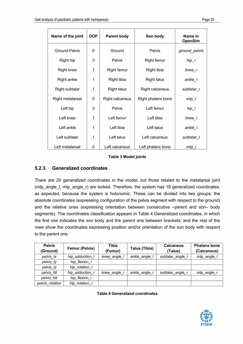
Name of the joint DOF Parent body Son body Name in OpenSim
Ground-Pelvis 6 Ground Pelvis ground_pelvis
Right hip 3 Pelvis Right femur hip_r
Right knee 1 Right femur Right tibia knee_r
Right ankle 1 Right tibia Right talus ankle_r
Right subtalar 1 Right talus Right calcaneus subtalar_r
Right metatarsal 0 Right calcaneus Right phalanx bone mtp_r
Left hip 3 Pelvis Left femur hip_l
Left knee 1 Left femur Left tibia knee_l
Left ankle 1 Left tibia Left talus ankle_l
Left subtalar 1 Left talus Left calcaneus subtalar_l
Left metatarsal 0 Left calcaneus Left phalanx bone mtp_l
Table 3 Model joints
5.2.3. Generalized coordinates
There are 20 generalized coordinates in the model, but those related to the metatarsal joint
(mtp_angle_l, mtp_angle_r) are locked. Therefore, the system has 18 generalized coordinates,
as expected, because the system is holonomic. These can be divided into two groups: the
absolute coordinates (expressing configuration of the pelvis segment with respect to the ground)
and the relative ones (expressing orientation between consecutive –parent and son– body
segments). The coordinates classification appears in Table 4 Generalized coordinates, in which
the first row indicates the son body and the parent one between brackets; and the rest of the
rows show the coordinates expressing position and/or orientation of the son body with respect
to the parent one.
Pelvis (Ground) Femur (Pelvis) Tibia
(Femur) Talus (Tibia) Calcaneus (Talus)
Phalanx bone (Calcaneus)
pelvis_tx hip_adduction_l knee_angle_l ankle_angle_l subtalar_angle_l mtp_angle_l pelvis_ty hip_flexion_l pelvis_tz hip_rotation_l pelvis_tilt hip_adduction_r knee_angle_r ankle_angle_r subtalar_angle_r mtp_angle_r pelvis_list hip_flexion_r
pelvis_rotation hip_rotation_r
Table 4 Generalized coordinates
Gait analysis of paediatric patients with hemiparesis Page 26
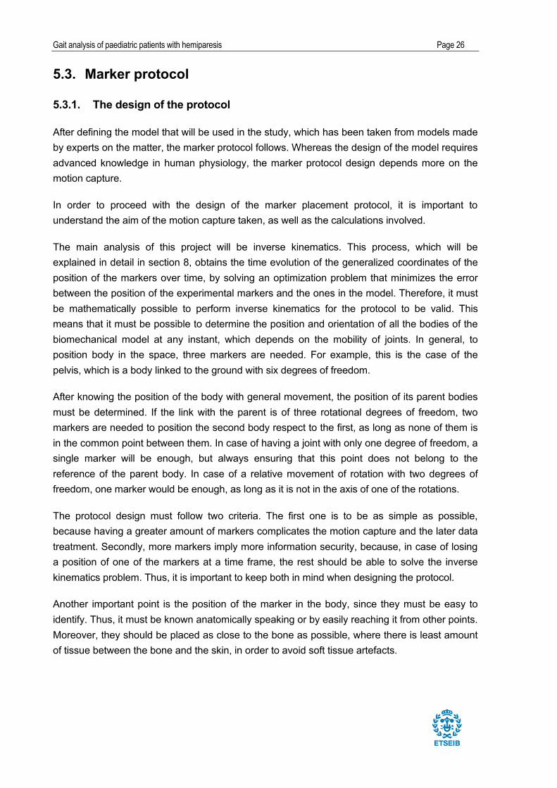
5.3. Marker protocol
5.3.1. The design of the protocol
After defining the model that will be used in the study, which has been taken from models made
by experts on the matter, the marker protocol follows. Whereas the design of the model requires
advanced knowledge in human physiology, the marker protocol design depends more on the
motion capture.
In order to proceed with the design of the marker placement protocol, it is important to
understand the aim of the motion capture taken, as well as the calculations involved.
The main analysis of this project will be inverse kinematics. This process, which will be
explained in detail in section 8, obtains the time evolution of the generalized coordinates of the
position of the markers over time, by solving an optimization problem that minimizes the error
between the position of the experimental markers and the ones in the model. Therefore, it must
be mathematically possible to perform inverse kinematics for the protocol to be valid. This
means that it must be possible to determine the position and orientation of all the bodies of the
biomechanical model at any instant, which depends on the mobility of joints. In general, to
position body in the space, three markers are needed. For example, this is the case of the
pelvis, which is a body linked to the ground with six degrees of freedom.
After knowing the position of the body with general movement, the position of its parent bodies
must be determined. If the link with the parent is of three rotational degrees of freedom, two
markers are needed to position the second body respect to the first, as long as none of them is
in the common point between them. In case of having a joint with only one degree of freedom, a
single marker will be enough, but always ensuring that this point does not belong to the
reference of the parent body. In case of a relative movement of rotation with two degrees of
freedom, one marker would be enough, as long as it is not in the axis of one of the rotations.
The protocol design must follow two criteria. The first one is to be as simple as possible,
because having a greater amount of markers complicates the motion capture and the later data
treatment. Secondly, more markers imply more information security, because, in case of losing
a position of one of the markers at a time frame, the rest should be able to solve the inverse
kinematics problem. Thus, it is important to keep both in mind when designing the protocol.
Another important point is the position of the marker in the body, since they must be easy to
identify. Thus, it must be known anatomically speaking or by easily reaching it from other points.
Moreover, they should be placed as close to the bone as possible, where there is least amount
of tissue between the bone and the skin, in order to avoid soft tissue artefacts.

Gait analysis of paediatric patients with hemiparesis Page 27
5.3.2. Protocol used in the project
The protocol used for all the captures is based on the Plug-in Gait marker placement, by ©Vicon
Motion Systems, for the lower body. However, the thigh markers were deleted, due to the
anatomical inaccuracy of placement. Moreover, the shank bone (tibia) marker was relocated at
the tibial tuberosity below the knee. Finally, one marker was added on the toes. The protocol
then includes 18 markers, which are distributed and grouped as follows in Table 5 and
distributed as in Fig. 11, using the same names used in the OpenSim software:
Body Markers in the body
Pelvis
R.ASIS
L.ASIS
R.PSI
L.PSI
Right femur R.GreatTroch
R.Knee.Lat
Left femur L.GreatTroch
L.Knee.Lat
Right tibia (shank bone) R. Shank.Front
R.Ankle.Lat
Left tibia (shank bone) L.Shank.Front
L.Ankle.Lat
Right calcaneus R.Heel
Right metacarpal R.Toe.Lat
Left metacarpal L.Toe.Lat
Right phalanx R.Toe.Med
Left phalanx L.Toe.Med
Table 5. Names of the markers used in the protocol
Fig. 11. Distribution of the markers in the body

Gait analysis of paediatric patients with hemiparesis Page 28
6. Motion capture
6.1. The Biomechanics Laboratory
This sections presents the Biomechanics Laboratory of the UPC. It includes the description of
the equipment, along with its characteristics. It also includes the calibration methodology, which
is essential to ensure a precise motion capture.
6.1.1. Laboratory equipment
The UPC Biomechanics Laboratory, located in ETSEIB, involves a marker-based motion
capture system OptiTrackTM
from Natural Point, Inc.
It consists of 16 cameras, model V100:R2, equipped with IR (infrared light) LEDs. It is designed
to capture the position of points within the capture space from the emission of infrared light,
which is reflected in the markers (small spheres coated with a highly reflective fabric) fixed in the
body being analysed. Therefore, the reflected light is discreetly captured by an optical system of
cameras. Each of the cameras positions each marker in the perpendicular plane to its optical
axis. The capture frequency is 100 Hz (100 images/second).
Using all the information captured by several cameras, the system is capable of computing the
position of all the markers in the three-dimensional space. This information is processed by
obtaining the position in space of all the markers present in the capture space. A marker and a
camera can be seen in Fig. 12 and Fig. 13:
Fig. 12 OptiTrack Camera Fig. 13 Marker
The cameras are arranged as shown in Fig. 14 A view of the Biomechanics Laboratory around
the working space, eight located at three meters from the ground and six at a meter and a half.

Gait analysis of paediatric patients with hemiparesis Page 29
Fig. 14 A view of the Biomechanics Laboratory
The signals from the cameras are transferred to a computer through the hubs, which are USB
connection boxes where up to six cameras can be connected with USB 2.0 cables. These
signals are processed with the software Motive, which allows not only the capture of the
movement, but also the treatment of the captured data, as well as its export.
6.1.2. Calibration
In order to position the markers in the space, the camera system needs to be calibrated, which
involves both dynamic and static calibration.
The dynamic calibration is achieved by waving a calibration wand (Fig. 15) with three markers
attached to a pre-fabricated fixture in the work volume. Using the coincidental points and relative
distances of the three markers and by capturing them, the intrinsic and extrinsic parameters of
the camera system are calculated. The intrinsic parameters describe the variables that depend
on the camera optics, whereas the extrinsic ones describe the spatial pose of the camera. While
the wand is being moved, it is important to make sure that all the cameras are able to draw the
path made with the wand, which can be seen on the computer screen. Each camera records in
the plane perpendicular to its optical axis, thus in two dimensions. With the 2D images of all the
cameras the three-dimensional image is created.

Gait analysis of paediatric patients with hemiparesis Page 30
With the static calibration, the position and orientation of the camera with respect to the inertial
coordinate system is determined. An L-shaped plate equipped with three markers set at a pre-
defined distanced is placed on the floor at the centre of the volume that the motion captures
takes place, which is seen in Fig. 16.
Fig. 15 Calibration wand
Fig. 16 L-shaped plate with three markers

Gait analysis of paediatric patients with hemiparesis Page 31
6.2. Procedure for motion capture
Given the fact that how cerebral palsy affects varies from one patient to another, even when
having the same pathology (in this case, hemiparesis), this project is aimed to study each
patient independently. However, a similar procedure has been followed to capture the
movement of all subjects.
The capture of movement can be divided into four parts:
1. Static capture: it is used to scale the model when using the OpenSim software.
2. Natural gait (N): to show how the patient walks in their everyday life. It also allows the
physiotherapist to evaluate how he should set the parameters of the device for the
feedback.
3. Gait with feedback (F): after having the patient using the device for a while, it shows
how it modifies their gait pattern. For patient Isabel, there will be two feedbacks
(referred to as F1 and F2).
4. Gait right after the feedback (A): by stopping the feedback of the device, it shows if the
gait pattern has changed compared to the natural one after using it for a while.
Since every patient is different, the feedback chosen for each case will vary. Moreover, in the
case of one of the patients, Isabel, who has stability problems and more difficulty to walk, the
gait after the feedback could not be analysed, due to her exhaustion. However, two different
feedback cases for this case were taken, which are noted on.
As explained earlier when talking about the Walking O’Clock device, the physiotherapist chose
the feedback that had to be set. In the table below, the feedback used in each patient is shown
in Table 6:
Patient Feedback
Maria Flexion of 20° on right leg (F)
Jordi Flexion of 25° on left leg (F)
Isabel 1. Extension of 0° on right leg (F1)
2. Flexion of 20° on right leg (F2)
Table 6. Feedback used in each patient
Gait analysis of paediatric patients with hemiparesis Page 32
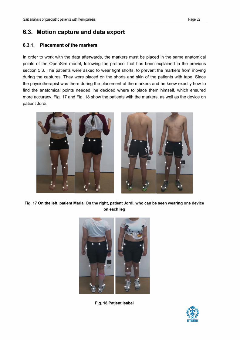
6.3. Motion capture and data export
6.3.1. Placement of the markers
In order to work with the data afterwards, the markers must be placed in the same anatomical
points of the OpenSim model, following the protocol that has been explained in the previous
section 5.3. The patients were asked to wear tight shorts, to prevent the markers from moving
during the captures. They were placed on the shorts and skin of the patients with tape. Since
the physiotherapist was there during the placement of the markers and he knew exactly how to
find the anatomical points needed, he decided where to place them himself, which ensured
more accuracy. Fig. 17 and Fig. 18 show the patients with the markers, as well as the device on
patient Jordi.
Fig. 17 On the left, patient Maria. On the right, patient Jordi, who can be seen wearing one device on each leg
Fig. 18 Patient Isabel

Gait analysis of paediatric patients with hemiparesis Page 33
6.3.2. Optical tracking
Using the software OptiTrack Motive the position of the markers during the capture is tracked.
Before starting the motion capture, the calibration file, which has been explained in section 3.2,
must be loaded. Once the patient is standing in the working area, all the markers must be seen
by the cameras. This is easy to check, because the software shows the number of markers that
it is tracking and where they are, which is useful in case one of them falls. Also, it is important to
remove any objects that may interfere with the cameras, such as jewellery or shiny materials.
One checked, the motion capture can start.
6.3.3. The walking path
Before starting the motion capture, a static pose capture was taken, which would be used for
the data processing afterwards (in order to use it to scale the model in the software OpenSim,
which is explained in 8.2). Then, each patient was asked to walk from one side of the
Laboratory to the other side straight ahead, trying to do it in their regular speed. They could use
the pressure plate as a visual reference, which were not used in this project, in order to keep a
straight line. As seen in the left picture, there were two marks on the ground, which the patients
could use to know where to start and turn to walk. In each walk from side to side, one capture
was recorded, which it included, at least, three gait cycles. The same procedure was followed
for every part for every patient. Fig. 19 shows patient Jordi going back and forth through the
chosen path.
Fig. 19 Jordi path

Gait analysis of paediatric patients with hemiparesis Page 34
6.3.4. Write the TRC file
In order to ensure a precise analysis of the gait pattern of every part, several captures were
taken for each patient. For each of the parts (listed in section 6.2), three captures have been
chosen, except from the static one, which was complete with only one capture. Therefore, ten
captures per patient have been processed.
First of all, the captures had to be edited before being exported from the Laboratory Software,
Motive. All the markers had to be named and checked. In case a marker was missing or had
been lost by the program during a period of frames in the capture, the gap was filled with the
editing tool fill gaps. Also, if the cameras lost a marker during the capture and it appeared as a
new one, it was merged with the corresponding one with the editing tool merge markers. All of
this had to be done manually and making sure not to miss any marker, or else the file would not
be worked on with the software.
The files then were exported as a .csv file extension. That file would be then transformed into a
.trc file, which is the one that the software OpenSim reads. To do so, a Matlab program was
created and used, which directly converted the files into .trc, just by executing them. Basically,
what it did was:
1. Read the .csv file and create one with Matlab extension
2. Read all number of the file, along with the information about rows and columns
3. Read how many markers would be in the capture and the corresponding names
4. Adjust the axes:
x_OpenSim=z_cameras
y_OpenSim=y_cameras
z_OpenSim=-x_cameras
The files are then ready to be opened with the OpenSim software.

Gait analysis of paediatric patients with hemiparesis Page 35
7. Kinematics analysis
7.1. Introduction to OpenSim
This section explains the main options of OpenSim 3.1, which is the program that has been
used to perform kinematic calculations. Once the program has been opened and the model
loaded, the interface looks as seen in Fig. 20:
Fig. 20 OpenSim user interface
The browser (Navigator) allows choosing which elements are displayed, having the options of
Bodies, Joints or Markers. Moreover, by clicking the right mouse button, several display actions
are unfolded. More than one model can be added in the browser, but only one can be active,
which is achieved by clicking on the Make Current option.
All the tools for the analysis of motion are included on the Tools menu. The ones used in this
project are the following:
• Scale model: based on a generic model skeleton, it transforms its dimensions to those of
the subject of the capture.
• Inverse Kinematics: it calculated the value of the generalized coordinates over time from
the marker position measurements.
Gait analysis of paediatric patients with hemiparesis Page 36
7.2. Scaling the model
The first step for the motion analysis is to scale the model, in order to create a skeleton model
as close as possible to the real subject. In addition, it allows relocating the markers in the model
in most similar way to how they were placed in reality. It is advisable to relocate them (Adjust
Markers Model) once the model has already been adjusted and, therefore, the size is the
appropriate one.
For this process, two files are necessary: the file with the generic model that will be modified
(.osim) and the file motion capture that will enable the changes (.trc). The result of the scaling is
a scaled new model, with the extension .osim, that can be saved for later use.
The process starts by going on the Tools menu > Scale Model. The first step is to specify the
mass of the model, which is adjusted for each subject according to their total mass. The mass is
needed for the analysis of dynamics. Thus, it is not essential in this project, since it will only take
into account the analysis of kinematics, but, this way, the model is adjusted and scaled properly.
This mass will be distributed segment by segment in proportion to the original model. Therefore,
in the Scale Model section, the option Preserve mass distribution during scale must be active
and the direction of the .trc file of the static pose must be indicated. In the first scale, the Adjust
Model Markers must be deactivated, to only change the dimensions of the skeleton and not the
position of the sensors in the model.
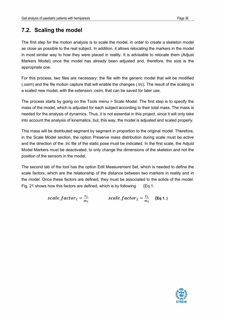
The second tab of the tool has the option Edit Measurement Set, which is needed to define the
scale factors, which are the relationship of the distance between two markers in reality and in
the model. Once these factors are defined, they must be associated to the solids of the model.
Fig. 21 shows how this factors are defined, which is by following (Eq 1:
#$%&'_)%$*+,- = '-/-#$%&'_)%$*+,1 = '1
/1 (Eq 1. )

Gait analysis of paediatric patients with hemiparesis Page 37
Fig. 21 Distance of two markers. On the left, experimental markers. On the right, markers from the model. Taken from the OpenSim guide [2].
There is the option to scale the segments with the same factor in all three directions or
discriminate different factors in different directions. This depends on the markers used and how
they can be related. Fig. 22 shows the markers pairs for the measurements used to apply the
scale factors. Fig. 23 shows the applied scale factors that OpenSim has then calculated.
Fig. 22 Marker pairs for the measurements used to scale

Gait analysis of paediatric patients with hemiparesis Page 38
Fig. 23 The applied scale factors for each body and the measurements used
In Fig. 24, the changes in the model after the scale are noticed, since the patient is shorter, her
pelvis is wider and, thus the legs are further apart.
Fig. 24 On the left, the generic model. On the right, the scaled model.
After the skeletal model scale is done, the option Adjust Model Markers follows, to relocate the
markers as similar to where they were in reality as possible from a .trc file. In the Static Pose Weights, it is desirable to set different weights on the markers, since this is the weight that each
marker will have in the optimization carried to adjust its position. Low weight markers are those
with less precise positions, due to being away from the bone and with the possibility of soft
tissue movements. On the other hand, high weight markers are those with a precise anatomic
location. The chosen weights can be seen in Fig. 25:

Gait analysis of paediatric patients with hemiparesis Page 39
Fig. 25 Static Pose Weights for each marker
To check whether the scale process has been successful, the experimental markers of the
static pose can superimpose the model. To do so, inverse kinematics of the static pose must be
done first for the scaled model (this process will be in detail explained further). Once done, on
the section Motions of the OpenSim browser a file named Results appears. This file must be
linked to the experimental markers, by clicking on the Results file with the right mouse button
and selecting Associate Motion Data, adding then the .trc file of the static pose. Fig. 26 shows
this association, where the two markers can be seen and it is visible that the scale process was
satisfactory:
Fig. 26 On the left, the scaled lower body model, with model (pink) and experimental (blue) markers. On the right, a closer view of the feet.
Gait analysis of paediatric patients with hemiparesis Page 40
7.3. Inverse kinematics
Once the model is scaled and adjusted for the patient that is being analysed, the kinematics of
the system bodies can be obtained through inverse kinematics. This tool, which is called Inverse Kinematics in OpenSim, uses the .trc file of the motion capture to obtain the evolution of the
generalized coordinates over time. The resulting file is a Motion file (.mot extension), which
contains the value of the generalized coordinates of the model in every instant of the capture.
7.3.1. Calculation of inverse kinematics
Inverse kinematics solve an optimization problem, based on minimizing the distance between
the positon of the markers of the OpenSim skeletal model and the experimental markers placed
in the body of the patient for every instant of time. Thus, the objective function to be minimized
is (Eq 2. :
/234 52 6789: − 67(=)1/
2?- (Eq 2.)
Being @2(4) the position vector of the ith marker of the OpenSim skeleton model, which
depends on the system configuration described by the vector of the generalized coordinates 4.
Moreover, @2'@A
is the position vector of the ith experimental marker (placed in the body of the
patient). Finally, B7 is the weight assigned to the ith marker. As mentioned, this weight is the
degree of importance given to the markers, depending on how clear their position in the body is.
Thus, the markers with more weight will be those whose location is more precisely defined,
whereas the others will be the ones with less clear points anatomically speaking or that can
have more soft tissue movement (i.e., those that are away from the bone).
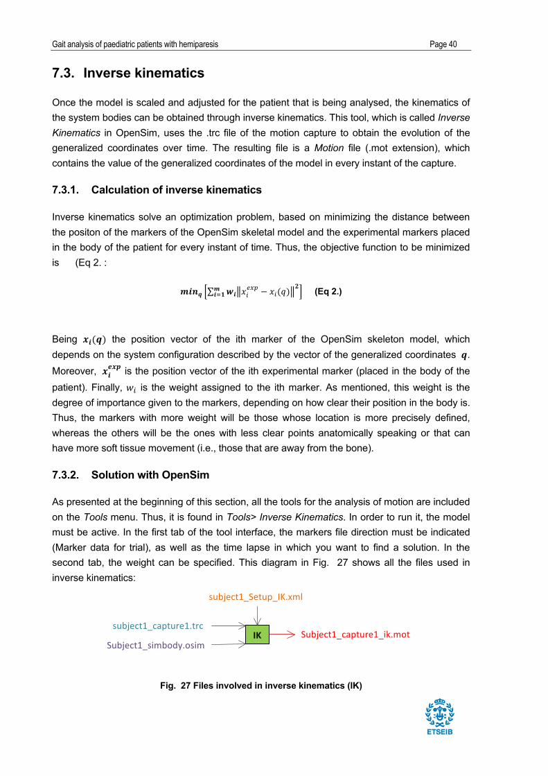
7.3.2. Solution with OpenSim
As presented at the beginning of this section, all the tools for the analysis of motion are included
on the Tools menu. Thus, it is found in Tools> Inverse Kinematics. In order to run it, the model
must be active. In the first tab of the tool interface, the markers file direction must be indicated
(Marker data for trial), as well as the time lapse in which you want to find a solution. In the
second tab, the weight can be specified. This diagram in Fig. 27 shows all the files used in
inverse kinematics:
IK subject1_capture1.trc
subject1_Setup_IK.xml
Subject1_simbody.osim Subject1_capture1_ik.mot
Fig. 27 Files involved in inverse kinematics (IK)

Gait analysis of paediatric patients with hemiparesis Page 41
The result is a .mot file with as many rows as frames had the captures, with the defined
coordinates of the model as columns. This result must be saved by clicking on the right button
of the Result file that appears on the Motions section of the browser.
When the kinematics is done, the Messages window of OpenSim shows the report of the
results, which evaluates the marker errors. It does it by finding the quadratic error between the
position of each experimental marker and its position in the model configuration resulting from
the inverse kinematics (Eq 3. :
'/%,C = 6789: − 67(=)1 (Eq 3.)
The errors can also be evaluated visually, by associating the file to the motion capture file, so it
shows the movement of the model and of the markers simultaneously. Moreover, OpenSim can
show the error of every marker for every frame. The maximum error should not exceed 2-4 cm
and the RMS value of the error cannot be greater than 2 cm, for all the markers.
Gait analysis of paediatric patients with hemiparesis Page 42
8. Results and discussion
This chapter presents the results obtained from the motion capture, and an analysis of these
data. It first starts with the methodology followed to treat all the data obtained from the software
OpenSim. Afterwards, the four generalized coordinates of the sagittal plane will be analysed for
each patient.
8.1. Methodology
After executing the inverse kinematics in the OpenSim software, the generalized coordinates of
each capture were exported to a .mot file. In order to read this file, a Matlab program was
created. Since the objective of this project is to analyse how the gait pattern changes when
using the Walking o’Clock device, one gait cycle of each capture will be analysed. The
methodology followed for the three patients will be explained in this section.
First of all, when any of the captures was exported from the Motive software, as explained in
section 7, it had a number of frames, which is equivalent to the time that the capture had been
recorded. Since every capture had at least three complete gait cycles, it was essential to know
from which frame to which frame the wanted gait cycle goes, in order to identify it from the
whole motion capture. As mentioned in 4.3.2 with more detail, the gait cycle starts when one
foot touches the ground (IC), and the cycle finishes when the same foot touches de ground
again. In the study, the right foot was taken as the reference. Therefore, when the subject
stepped on his/her right foot, the gait cycle started, ending with the same right foot stepping
back on the ground. To decide which frames are included in the chosen gait cycle, the y axis of
the right heel was plotted on Matlab. This way, the frames could be chosen by looking at when
the y axis of the right heel marker reached the minimum value. The information of the marker
was imported from the .csv file taken from the Motive software, which is read in Matlab.
Fig. 28 shows how the frames of the gait cycle for the first natural motion capture of patient
Maria were defined. The cursors show that it starts at frame 63 and ends at frame 181. The
same procedure is followed for all the other captures. These frames will be used in all the
programs created to analyse every capture.

Gait analysis of paediatric patients with hemiparesis Page 43
Fig. 28 The plot that shows the coordinate y of the position of the right foot with the frame. N1, Maria
The following Table 7 shows the chosen frames for all the captures. On the first column appears
the name of the capture, on the second one the initial frame (IF) and on the third the final frame
(FF). The names of the captures are the ones defined in 7.1
Patient
Maria Jordi Isabel
Capture IF FF Capture IF FF Capture IF FF
N1 61 177 N1 160 275 N1 401 588
N2 194 310 N2 116 228 N2 274 488
N3 173 290 N3 74 177 N3 378 558
F1 283 410 F1 158 269 F11 585 786
F2 109 214 F2 123 229 F12 153 327
F3 45 155 F3 176 285 F13 677 839
A1 43 155 A1 209 325 F21 425 580
A2 89 207 A2 170 283 F22 618 798
A3 208 327 A3 163 279 F23 410 596
Table 7. Initial and final frames of the analysed gait cycles for each motion capture.
Having the frames, the methodology followed with all the gait cycles was the same for the three
patients, but always separately. As commented, this project studies the kinematics of gait and
only the angular coordinates in the sagittal plane will be analysed. These are:

Gait analysis of paediatric patients with hemiparesis Page 44
• Pelvic tilt angle
• Right and left knee angles
• Right and left hip angles
• Right and left ankle angles
The analysis steps followed are the following:
1. Plotting the coordinates of each gait cycle and checking that all the values are logical
2. Calculating the maximum and minimum angles of each gait cycle. Since the
physiotherapist took the maximum and minimum angles of the thigh (considered as hip
flexion angles as explained in section 4) to think of the best feedback for the patient, it is
interesting to compare them.
a. For each phase, find the mean value for the maximum and minimum angle (3
per patient)
b. With the mean values, find the ROM of each phase and the percentage that has
changed from the natural gait
3. Finding the equation that describes each coordinate for each gait cycle and generate the
mean for each phase. Then, for each coordinate, three plots are expected (for example,
in the case of patient Maria, one for the natural phase, one for the feedback phase and
one for the after feedback phase)
4. To calculate the Root Mean Square Error (RMSE) comparing the three phases.
a. For patients Maria and Jordi, three RMSE will be calculated:
i. Natural pattern vs Feedback
ii. Natural pattern vs After Feedback
iii. Feedback vs After Feedback
b. For patient Isabel two RMSE will be calculated:
i. Natural pattern vs Feedback 1
ii. Natural pattern vs Feedback 2
5. To merge the plots of the three phases and compare them.
There are different facts that are important to mention. First of all, when proceeding with the
inverse kinematics, some abnormalities were seen, since the pelvis took a position impossible

Gait analysis of paediatric patients with hemiparesis Page 45
to reach in reality (completely twisted). After having investigated the captures that presented this
problem, the cause was found as being a problem of the direction of the walk. As explained in
section 7.2.3, the patients first walked to one side and then came back. Therefore, when they
came back, since they rotated the pelvis completely, the model got confused. This was solved
by directly changing the model and broadening the limit values of these coordinates.
After the inverse kinematics, when calculating the maximum and minimum angles, another
abnormality appeared in some cases, such as angles that could not be possible in reality.
Therefore, by looking back at the performance of the inverse kinematics tool in OpenSim, the
problem was visible. By checking the captures that had problems with the angles, it could be
seen that they reached limit values in the coordinates of OpenSim. This was also solved by
changing the limit values for the coordinates that gave problems.
It is important to keep in mind that the constrains given to the generalized coordinates only
affect the dynamics of the capture, not the inverse kinematics, so the values can be changed as
wanted with no consequences in this case.
This problem may be due to that, when the capture was taken, the patient may have not walked
perfectly straight. Also, given the fact that the patients may present deformities in their skeleton,
OpenSim may get confused. In addition, there were a couple of captures that kept giving wrong
angles, even having changed the model. In these cases, the solution was to go back to the
Motive software and export new captures of the same phase in substitution of the abnormal
one. For these new captures, the same methodology had to be followed.
Another problem that appeared in some captures was that, after analysing them, an odd
behaviour was seen, compared to the other captures of the same gait, such as unexpected
peaks. Therefore, after trying to understand the cause of such behaviour without success, the
solution taken was to change the gait cycle chosen from that capture, by taking the one before
or after (changing then the frames), so that the capture itself was not changed.
As mentioned before, the three patients will be analysed separately. The objective is to compare
the three different phases for each of them. Moreover, the shape of the plots of the studies
coordinates will be visually compared to the standard ones, presented in 4.3.2. However, since
it is a fact that the patients have a pathology that modifies their gait pattern, it is expected that it
will vary from the standard one. Then, it may allow seeing if the affected leg approaches the
standard pattern with the use of the device. For each patient, the four above-mentioned
coordinates will be analysed by analysing the maximum and minimum angles, the motion range
and the graphs representing the three phases, along with the RMSE.

Gait analysis of paediatric patients with hemiparesis Page 46
8.2. Maria
Patient Maria was put under a feedback of 20º angle of the right thigh (considered as hip
flexion).
8.2.1. Hip flexion
Fig. 29 and Fig. 30 show the hip flexion angle pattern for both legs in a GC:
Fig. 29. Non-affected hip flexion angle in a GC
Fig. 30. Affected hip flexion angle in a GC

Gait analysis of paediatric patients with hemiparesis Page 47
Coordinate Angle type Natural Feedback After feedback
Affected hip flexion
max 40,39 38,37 38,37min 0,64 -5,63 -8,64
Non-affected hip flexion
max 31,81 32,63 35,76min -6,31 -0,32 -4,12
Table 8. Maximum and minimum angles of hip flexion in a GC
Coordinate Natural Feedback After
feedback %F/N %A/N
Affected hip flexion
39,75
44,00
47,01
10,69
18,27
Non-affected hip flexion
38,12
32,95
39,88
-13,57
4,62
Table 9. Hip ROM
As seen in Table 8, the maximum angle for the affected and non-affected hip flexion has not
had an important variation with the feedback. The difference appears when it comes to
minimum angles for both legs. Whereas the minimum angle is greater (in absolute value) for the
affected hip, it decreases for the non-affected one during the feedback.
The ROM for the hip of the affected limb has increased in both cases (F and A, see Table 9). It
is interesting to notice that, during the feedback, while the affected hip increased its ROM, the
non-affected one decreased it. When looking at the ROM for both hips during feedback, the
difference is of more than 10°. In this case, the patient moved more the affected hip.
When looking at the pattern of all the captures, it is visible that the affected limb is the one that
suffers most change with respect to the natural motion. This is also backed up with the RMSE
Coordinate Natural-
Feedback Natural-After
feedback Feedback-After
feedback
Affected hip flexion
5,70
7,31
2,12
Non-affected hip flexion
3,43
2,39
2,97
Table 10. RMSE between phases
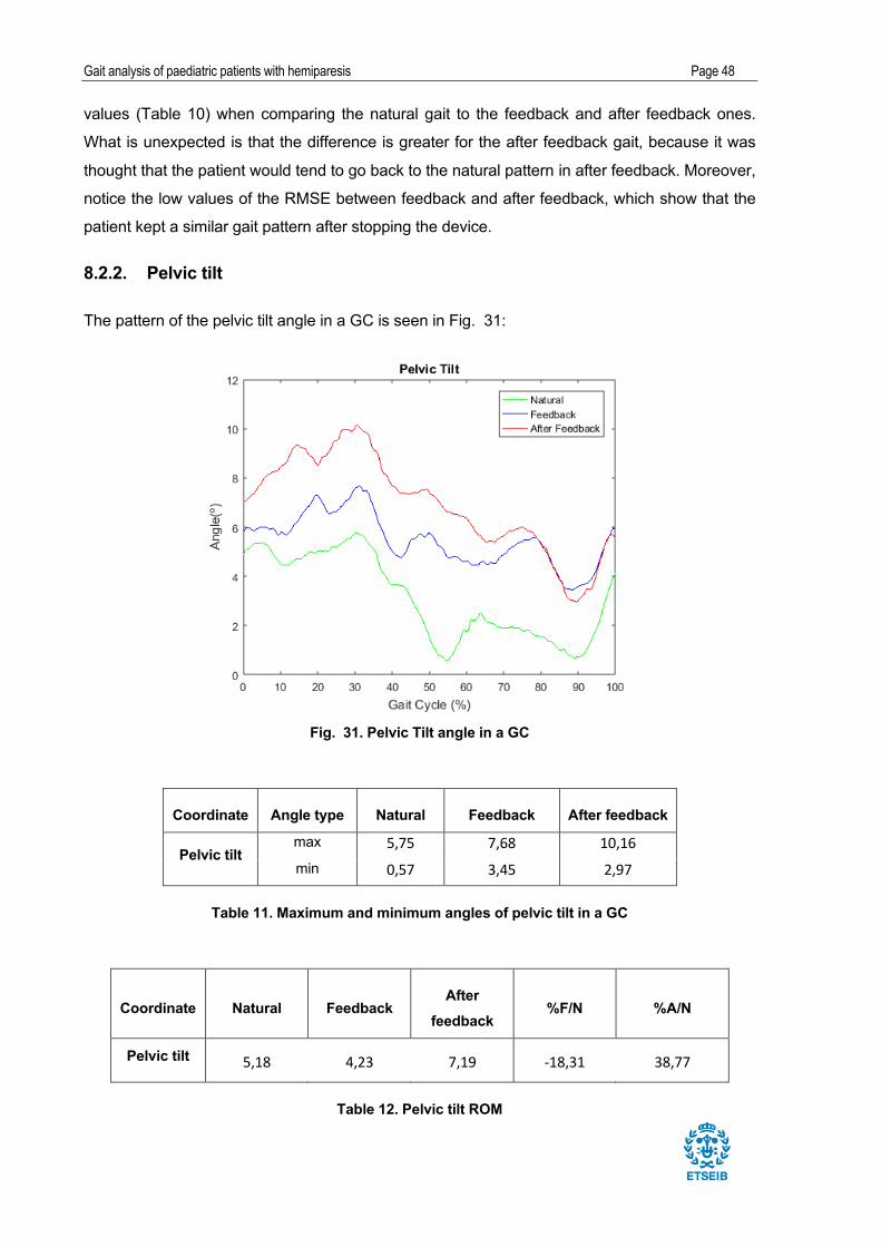
Gait analysis of paediatric patients with hemiparesis Page 48
values (Table 10) when comparing the natural gait to the feedback and after feedback ones.
What is unexpected is that the difference is greater for the after feedback gait, because it was
thought that the patient would tend to go back to the natural pattern in after feedback. Moreover,
notice the low values of the RMSE between feedback and after feedback, which show that the
patient kept a similar gait pattern after stopping the device.
8.2.2. Pelvic tilt
The pattern of the pelvic tilt angle in a GC is seen in Fig. 31:
Fig. 31. Pelvic Tilt angle in a GC
Coordinate Angle type Natural Feedback After feedback
Pelvic tilt max 5,75 7,68 10,16min 0,57 3,45 2,97
Table 11. Maximum and minimum angles of pelvic tilt in a GC
Coordinate Natural Feedback After
feedback %F/N %A/N
Pelvic tilt 5,18 4,23 7,19 -18,31 38,77
Table 12. Pelvic tilt ROM

Gait analysis of paediatric patients with hemiparesis Page 49
Coordinate Natural-
Feedback Natural-After
feedback Feedback-
After feedback
Pelvic tilt 2,56 3,95 1,81
Table 13. RMSE between phases
Notice that the maximum angles increase in both feedbacks (Table 11). However, the minimum
angles also increase in value, shifting the pattern upwards, as seen in Fig. 31. During feedback,
the pelvic tilt pattern is closer to the standard one, which is supported by the lower ROM (Table
12). This fact indicates that the patient gains stability when using the device. However, in after-
feedback, ROM is higher than in natural gait, so the patient loses stability. This may be due to
the transition between states and the confusion that may have caused her. As for hip flexion,
the RMSE value between feedback and after feedback is low (Table 13).
8.2.3. Knee flexion
Fig. 32 and Fig. 33 show the knee flexion angle pattern in a GC for both legs:
Fig. 32. Affected knee flexion angle in a GC

Gait analysis of paediatric patients with hemiparesis Page 50
Fig. 33. Non-affected knee flexion angle in a GC
Coordinate Angle type Natural Feedback After feedback
Affected knee flexion
max 70,22 65,85 64,69min 22,62 5,20 -3,20
Non-affected knee flexion
max 62,97 60,26 58,84min 7,33 7,89 6,75
Table 14. Maximum and minimum angles of knee flexion in a GC
Coordinate Natural (N) Feedback
(F) After
feedback (A) %F/N %A/N
Affected knee flexion 47,60 60,65 67,89 27,42 42,63
Non-affected knee flexion 55,64 52,37 52,10 -5,88 -6,37
Table 15. ROM of the knee flexion angle

Gait analysis of paediatric patients with hemiparesis Page 51
Coordinate Natural-
Feedback Natural-After
feedback Feedback-After
feedback
Affected knee flexion 16,60 22,57 6,49
Non-affected knee flexion 3,36 5,02 3,80
Table 16. RMSE between phases
There is a negative angle in after-feedback for the affected knee during stance (Table 14),
which means that there is genu recurvatum, also referred to as hyperextension [8].
While the knee ROM in the natural pattern is lower for the affected leg (Table 15), it becomes
greater with the feedback. The difference in ROM varies dramatically when using the device. As
seen in the graph above, it is obvious that this change occurs during the first phases of the gait
cycle, when the angle highly decreases. The non-affected limb does not present any important
changes when it comes to maximum and minimum angles, even though the ROM slightly
decreases with the feedback.
The most important difference of the knee flexion is for the affected limb. As easily seen in the
graphs, the affected knee angle presents a flat tendency during the first phases of gait, which is
known as stiff knee. As seen, the stiffness does not disappear when using the device, but it is
clearly modified and not as flat. Actually, the after feedback pattern resembles more the normal
shape than the other two. The RMSE values show the great difference between patterns for the
affected limb (Table 16).
8.2.4. Ankle dorsiflexion
In Fig. 34 and Fig. 35, the angle pattern for ankle dorsiflexion for both legs in a GC is seen:

Gait analysis of paediatric patients with hemiparesis Page 52
Fig. 34. Affected ankle dorsiflexion angle in a GC
Fig. 35. Non-affected ankle dorsiflexion angle in a GC

Gait analysis of paediatric patients with hemiparesis Page 53
Coordinate Angle type Natural Feedback After feedback
Affected ankle dorsiflexion
max 9,37 11,55 12,51min -31,05 -14,76 -15,50
Non-affected ankle dorsiflexion
max 23,59 22,47 22,74min -2,58 -4,77 -6,48
Table 17. Maximum and minimum angles of ankle dorsiflexion in a GC
Coordinate Natural
(N) Feedback
(F) After
feedback (A) %F/N %A/N
Affected ankle dorsiflexion
40,42 26,31 28,01 -34,91 -30,71
Non-affected ankle dorsiflexion
26,17 27,24 29,22 4,09 11,67
Table 18. ROM of the ankle dorsiflexion angle
Coordinate Natural-
Feedback Natural-After
feedback
Feedback-After
feedback
Affected ankle dorsiflexion
8,21 8,89 1,94
Non-affected ankle dorsiflexion
3,25 3,13 1,26
Table 19. RMSE between phases
The affected ankle, which has a larger minimum angle (in absolute value) in the natural gait, is
the most modified. The ROM greatly decreases and its value approaches the one of the non-
affected ankle.
Satisfactorily, the pattern of feedback and after feedback for the affected side is more similar to
the standard one. The abnormal peak that appeared in pre-swing of the GC disappears when
using the device, which shows more control of the ankle.
Also, an abnormal peak appears in the natural gait of the non-affected ankle during the terminal
swing of the GC, which softens with feedback. However, at the same point, a pronounced low
peak appears in the after feedback.

Gait analysis of paediatric patients with hemiparesis Page 54
8.3. Jordi
Patient Jordi was put under a feedback of 25º angle of the left thigh (considered as hip flexion).
8.3.1. Hip flexion
Fig. 36 and Fig. 37show the hip flexion angle pattern for both legs in a GC:
Fig. 36. Non-affected hip flexion angle in a GC
Fig. 37. Affected hip flexion angle in a GC

Gait analysis of paediatric patients with hemiparesis Page 55
Coordinate Angle type Natural Feedback After
feedback
Affected hip flexion
max 27,59 25,46 24,93min -6,48 -1,37 -1,26
Non-affected hip flexion
max 31,60 27,65 28,58min -9,84 -6,45 -6,27
Table 20. Maximum and minimum angles of hip flexion in a GC
Coordinate Natural (N) Feedback
(F) After
feedback (A) %F/N %A/N
Affected hip flexion 34,07 26,83 26,20 -21,25 -23,10
Non-affected hip flexion 41,44 34,10 34,85 -17,71 -15,89
Table 21. ROM of the hip flexion angle
Coordinate Natural-
Feedback Natural-After
feedback Feedback-
After feedback
Affected hip flexion 3,97 4,34 1,16
Non-affected hip flexion 3,02 2,87 1,33
Table 22. RMSE between phases
In this case, the feedback was set on the left leg, because the patient was over flexing the non-
affected hip (see Fig. 36). This is why the maximum angle for the left hip decreases with the
use of the device. Concurrently, as seen in Table 20, the hip angle during stance reached -6,5°,
which showed an over extension, which is compensated with the feedback. Moreover, for both
limbs, the ROM of the hip flexion decreases, which can be concluded as more control and
stability of both limbs (Table 21).
When looking at the plots, an abnormality is seen in all the patterns. In the swing phase of the

Gait analysis of paediatric patients with hemiparesis Page 56
GC of the affected leg, there is an unexpected double bump (seen from 60 to 95%), which is not
solved with the use of the device. This is due to the pathology of the patient.
Satisfactorily, the change in pattern between feedback and after feedback is not significant,
which is supported by the RMSE values (see Table 22). The gain of control in both limbs is
visual, because the peaks seen in the natural gait decrease with feedback and after feedback.
8.3.2. Pelvic tilt
The pattern of the pelvic tilt angle in a GC is seen in Fig. 38:
Fig. 38. Pelvic Tilt angle in a GC
Coordinate Angle type Natural Feedback After
feedback
Pelvic tilt max 4,06 0,89 2,90min -1,91 -2,01 -1,97
Table 23. Maximum and minimum angles of pelvic tilt in a GC

Gait analysis of paediatric patients with hemiparesis Page 57
Coordinate Natural (N) Feedback
(F) After
feedback (A) %F/N %A/N
Pelvic tilt 5,97 2,90 4,87 -51,35 -18,32
Table 24. ROM of the pelvic tilt angle
Coordinate Natural-
Feedback Natural-After
feedback Feedback-After
feedback
Pelvic tilt 2,61 0,98 2,36
Table 25. RMSE between phases
There is a significant peak (maximum angle) during natural gait (Table 23), which is lowered
with feedback. In addition, the ROM dramatically decreases with feedback (Table 24). It is also
clearly seen that the pattern is closer to the standard one (see figure Fig. 38). This is directly
related to gaining balance. When looking at the patterns and at the RMSE values (Table 25),
the patient went back to the pelvic tilt angle pattern when stopping the feedback. Thus, it looks
like he did not maintain the balance gained with feedback.
8.3.3. Knee flexion
Fig. 39 and Fig. 40 show the knee flexion angle pattern in a GC for both legs:
Fig. 39. Affected knee flexion angle in a GC

Gait analysis of paediatric patients with hemiparesis Page 58
Fig. 40. Non-affected knee flexion angle in a GC
Coordinate Angle type Natural Feedback After feedback
Affected knee flexion
max 66,81 62,18 62,08
min -6,44 -5,80 -3,27
Left knee flexion
max 75,65 64,80 67,28
min -4,18 4,24 3,86
Table 26. Maximum and minimum angles of knee flexion in a GC
Coordinate Natural
(N) Feedback (F)
After feedback (A)
%F/N %A/N
Affected knee flexion 73,25 67,98 65,35 -7,20 -10,80
Non-affected knee flexion 79,83 60,56 63,42 -24,14 -20,56
Table 27. ROM of the knee flexion angle

Gait analysis of paediatric patients with hemiparesis Page 59
Coordinate Natural-Feedback
Natural-After feedback
Feedback-After feedback
Affected knee flexion 5,57 6,13 2,67
Non-affected knee flexion 6,90 5,94 2,73
Table 28. RMSE between phases
As seen in Table 26, both knees present hyperextension in natural gait. Whereas it is
neutralized with feedback for the non-affected knee, it remains for the affected one.
As it happened with the hip flexion, the ROM decreases for both knees (Table 27). Whereas the
ROM for the affected knee was wider than the one for the non-affected knee, they are more
similar with the use of the device. Actually, the ROM of the non-affected knee is the one that
changes more, which would be expected, since it was the limb under feedback. This shows how
the patient gains control during the gait.
The non-affected knee presents a decreased ROM of the knee throughout the entire GC
compared to the standard one. In the swing period, there is a diminished and delayed peak
knee flexion (notice the flat pattern), which prevents not only normal limb clearance but also the
foot from being placed in the proper position prior to the next foot contact [8]. This is called stiff-
knee pattern. Even though the feedback was set on this limb, the stiffness remains with the use
of the feedback.
When looking at Table 28, the changes in pattern with feedback are maintained in after
feedback. Moreover, when looking at the pattern in both Fig. 39 and Fig. 40, the changes are
visually seen. It shows more control of knee flexion.
8.3.4. Ankle dorsiflexion
In Fig. 41 and Fig. 42, the angle pattern for ankle dorsiflexion for both legs in a GC is seen:

Gait analysis of paediatric patients with hemiparesis Page 60
Fig. 41. Affected ankle dorsiflexion angle in a GC
Fig. 42. Non-affected ankle dorsiflexion angle in a GC
Coordinate Angle type Natural Feedback After
feedback
Affected ankle dorsiflexion
max 6,17 2,69 3,01min -31,90 -28,06 -28,17
Non-affected ankle dorsiflexion
max 16,51 13,42 13,29min -16,37 -11,06 -11,32
Table 29. Maximum and minimum angles of ankle dorsiflexion in a GC
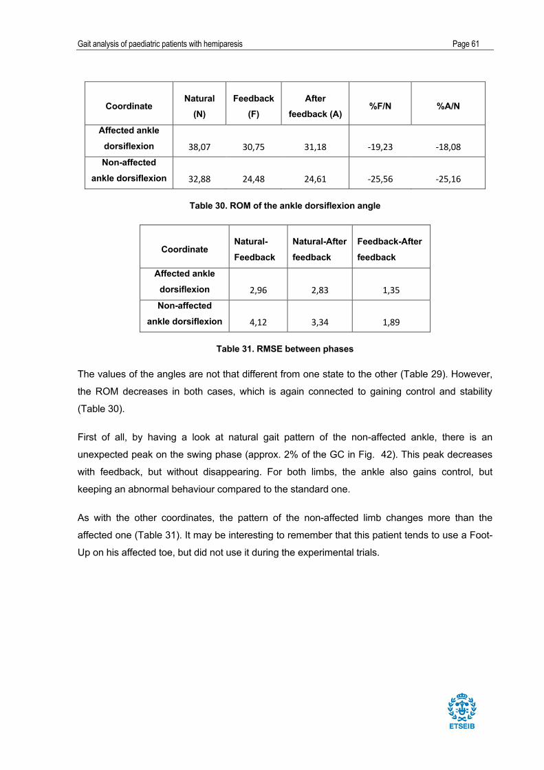
Gait analysis of paediatric patients with hemiparesis Page 61
Coordinate Natural
(N) Feedback
(F) After
feedback (A) %F/N %A/N
Affected ankle dorsiflexion 38,07 30,75 31,18 -19,23 -18,08Non-affected
ankle dorsiflexion 32,88 24,48 24,61 -25,56 -25,16
Table 30. ROM of the ankle dorsiflexion angle
Coordinate Natural-Feedback
Natural-After feedback
Feedback-After feedback
Affected ankle dorsiflexion 2,96 2,83 1,35Non-affected
ankle dorsiflexion 4,12 3,34 1,89
Table 31. RMSE between phases
The values of the angles are not that different from one state to the other (Table 29). However,
the ROM decreases in both cases, which is again connected to gaining control and stability
(Table 30).
First of all, by having a look at natural gait pattern of the non-affected ankle, there is an
unexpected peak on the swing phase (approx. 2% of the GC in Fig. 42). This peak decreases
with feedback, but without disappearing. For both limbs, the ankle also gains control, but
keeping an abnormal behaviour compared to the standard one.
As with the other coordinates, the pattern of the non-affected limb changes more than the
affected one (Table 31). It may be interesting to remember that this patient tends to use a Foot-
Up on his affected toe, but did not use it during the experimental trials.

Gait analysis of paediatric patients with hemiparesis Page 62
8.4. Isabel
Patient Isabel was put under two feedbacks; one of 0º angle (F1) and one of 20º (F2) of the right
thigh (considered as hip flexion).
8.4.1. Hip flexion
Fig. 43 and Fig. 44 show the hip flexion angle pattern for both legs in a GC:
Fig. 43. Non-affected hip flexion angle in a GC
Fig. 44. Affected hip flexion angle in a GC

Gait analysis of paediatric patients with hemiparesis Page 63
Coordinate Angle type Natural Feedback 1 Feedback 2
Affected hip flexion
max 28,37 24,58 27,97min -12,35 -11,63 -12,01
Non-affected hip flexion
max 26,11 18,76 25,85min -15,02 -15,58 -13,01
Table 32. Maximum and minimum angles of hip flexion in a GC
Coordinate Natural (N) Feedback 1 Feedback 2 %F1/N %F2/N
Affected hip flexion 40,72 36,22 39,98 -11,06 -1,83
Non-affected hip flexion 41,13 34,34 38,86 -16,51 -5,52
Table 33. ROM of the hip flexion angle
Coordinate Natural- Feedback1
Natural- Feedback2
Affected hip flexion 1,85 2,70
Non-affected hip flexion 3,94 2,65
Table 34. RMSE between phases
There is an interesting issue with the ROM (see Table 33). For feedback 1, even though more
for the non-affected limb, it decreases in both limbs and their final ranges of motion are similar.
Even though less significantly, it also decreases for feedback 2, also more for the non-affected
limb. For the peak values, there is not an important difference in feedback 2 (see Table 32).
However, the maximum angle for both limbs decreases in feedback 1, which is the one with the
angle set to 0°.
As commented above, the maximum angle decreases in feedback 1, but, when looking at the
RMSE value, the difference is greater for the non-affected hip (Table 34). Given the condition of
instability of the patient, feedback 1 seems to give her more control.
On the other hand, feedback 2 softens the peak in the terminal swing of the GC for the hip of
the affected limb, which approaches the standard hip flexion pattern.
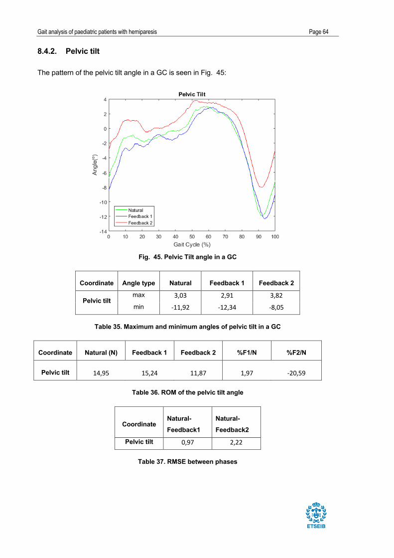
Gait analysis of paediatric patients with hemiparesis Page 64
8.4.2. Pelvic tilt
The pattern of the pelvic tilt angle in a GC is seen in Fig. 45:
Fig. 45. Pelvic Tilt angle in a GC
Coordinate Angle type Natural Feedback 1 Feedback 2
Pelvic tilt max 3,03 2,91 3,82min -11,92 -12,34 -8,05
Table 35. Maximum and minimum angles of pelvic tilt in a GC
Coordinate Natural (N) Feedback 1 Feedback 2 %F1/N %F2/N
Pelvic tilt 14,95 15,24 11,87 1,97 -20,59
Table 36. ROM of the pelvic tilt angle
Coordinate Natural- Feedback1
Natural- Feedback2
Pelvic tilt 0,97 2,22
Table 37. RMSE between phases

Gait analysis of paediatric patients with hemiparesis Page 65
When looking at Fig. 46, the pattern of feedback 2 looks similar to the other ones, but shifted
upwards. This is why the maximum angle of feedback 2 is greater (Table 35). This patient had
grave stability problems, which can be seen in the pelvic tilt pattern, which is far from the
standard one (shown in section 3.1). She could not walk for too long without resting.
For this reason, it is not surprising that the pelvic tilt pattern did not experience a great change
with any of the feedbacks, as can be seen by looking at the RMSE values (Table 37). In
However, when looking at Table 36, there is a great change in ROM with feedback 2. Thus, it
could be a sign of gaining stability, which is exactly what the patient needs.
8.4.3. Knee flexion
Fig. 46 and Fig. 47 show the knee flexion angle pattern in a GC for both legs:
Fig. 46. Affected knee flexion angle in a GC
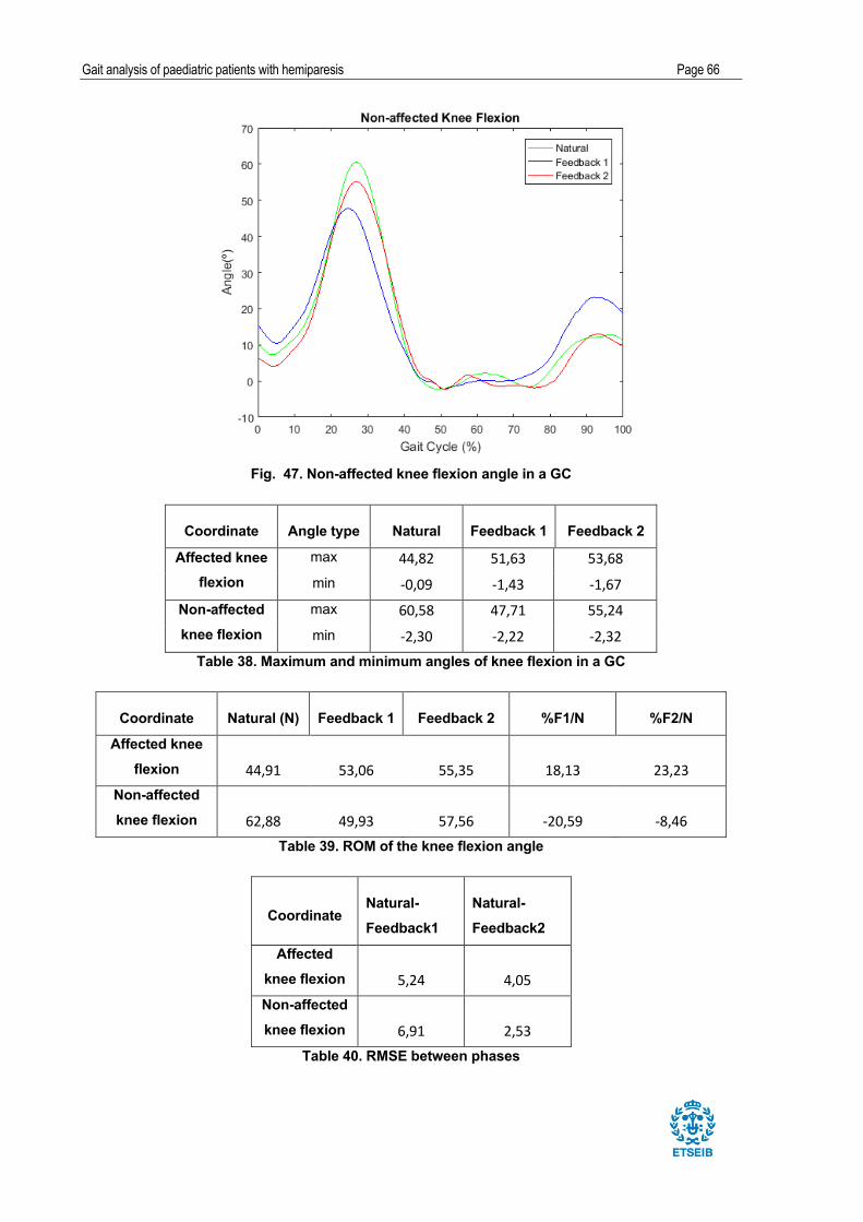
Gait analysis of paediatric patients with hemiparesis Page 66
Fig. 47. Non-affected knee flexion angle in a GC
Coordinate Angle type Natural Feedback 1 Feedback 2
Affected knee flexion
max 44,82 51,63 53,68min -0,09 -1,43 -1,67
Non-affected knee flexion
max 60,58 47,71 55,24min -2,30 -2,22 -2,32
Table 38. Maximum and minimum angles of knee flexion in a GC
Coordinate Natural (N) Feedback 1 Feedback 2 %F1/N %F2/N
Affected knee flexion 44,91 53,06 55,35 18,13 23,23
Non-affected knee flexion 62,88 49,93 57,56 -20,59 -8,46
Table 39. ROM of the knee flexion angle
Coordinate Natural- Feedback1
Natural- Feedback2
Affected knee flexion 5,24 4,05Non-affected knee flexion 6,91 2,53
Table 40. RMSE between phases

Gait analysis of paediatric patients with hemiparesis Page 67
It seems like there is compensation between both knees. Whereas the affected one gains ROM,
the non-affected one decreases it, thus both ranges become closer in values (Table 39). Thus,
gait becomes more symmetric. For feedback 2, the ROM are similar for both knees. Parallel,
when looking at Table 38, it is seen that maximum angle of the affected knee increases, then
flexing more, whereas the non-affected knee maximum angle decreases. In feedback 2, both
knees flex at a similar maximum angle.
The most relevant difference, which is seen visually, is that the double peak present in the
swing phase of the GC for the affected limb almost disappears with both feedbacks (see Fig.
46). For the affected limb, the knee flexion pattern is more similar to the standard one when
using both feedbacks. For the non-affected knee, feedback 1 is the one that affects the most in
terms of pattern, reducing more than 20% the knee flexion ROM. Also, the RMSE values (Table
40) show that both feedbacks seem to modify knee flexion pattern in a similar way for the
affected limb. In the case of the non-affected limb, feedback 1 modifies pattern more
significantly (also see Fig. 47).
8.4.4. Ankle dorsiflexion
In Fig. 48 and Fig. 49, the angle pattern for ankle dorsiflexion for both legs in a GC is seen:
Fig. 48. Affected ankle dorsiflexion angle in a GC

Gait analysis of paediatric patients with hemiparesis Page 68
Fig. 49. Non-affected ankle dorsiflexion angle in a GC
Coordinate Natural (N) Feedback 1 Feedback 2 %F1/N %F2/N
Affected ankle dorsiflexion 20,76 18,73 21,03 -9,78 1,32Non-affected
ankle dorsiflexion 28,14 31,32 26,60 11,29 -5,47
Table 42. ROM of the ankle dorsiflexion angle
Coordinate Angle type Natural Feedback 1 Feedback 2
Affected ankle dorsiflexion
max 1,33 0,30 2,17min -19,42 -18,43 -18,86
Non-affected ankle dorsiflexion
max 10,65 15,48 7,56min -17,50 -15,83 -19,04
Table 41. Maximum and minimum angles of ankle dorsiflexion in a GC

Gait analysis of paediatric patients with hemiparesis Page 69
Coordinate Natural- Feedback1
Natural- Feedback2
Affected ankle dorsiflexion 2,06 1,15
Non-affected ankle dorsiflexion 4,28 3,53
Table 43. RMSE between phases
Table 42 shows that the ROM of the non-affected ankle increases with feedback 1 and slightly
decreases with feedback 2, which does not modify it that much. Therefore, feedback 1 seems to
provide less stability, since the peak values create a pattern further from the standard one.
The plot of the affected ankle shows a completely different pattern from the standard one. This
is due to the fact that, as mentioned in section 5.3, the patient wears a DAFO, which
significantly affects the kinematic behaviour of that joint.
The non-affected ankle presents a low peak on the initial swing (at approx. 20% of the GC; see
Fig. 49), which decreases with both feedbacks. Both feedbacks seem to have the same effect
on the non-affected limb during the GC, except from the transition from stance to swing of the
GC, which seems to be better controlled for feedback 2.
As seen in Table 43, the RMSE values for the affected ankle show that both feedbacks have not
modified the pattern, which is logical when thinking of the DAFO. On the other hand, the non-
affected ankle dorsiflexion pattern is modified with both feedbacks, especially when it comes to
the peak mentioned above.

Gait analysis of paediatric patients with hemiparesis Page 70
9. Conclusions
The present Final Project for the Bachelor’s Degree in Industrial Technology Engineering has
analysed gait kinematics of paediatric patients with hemiparesis. It has been performed using
the UPC Biomechanics Laboratory located at ETSEIB. Thus, there has been a learning process
for the motion captures, along with all the used software: Motive, Matlab, and OpenSim. A
musculoskeletal model has been adapted from one developed by the OpenSim team.
There has been a biomedical involvement in the project. The focus has been on paediatric
hemiparesis, which is a form of cerebral palsy. Learning about the pathology and the effects that
it has on the patients has been crucial to better understand their gait behaviour. The project has
taken a different view than that of a regular engineering study, since these pathologies have
different effects on each patients and each of them must be treated separately. The four angular
coordinates that have been of interest for the study (pelvis tilt, hip flexion, knee flexion, ankle
dorsiflexion) define orientations in the sagittal plane.
A prototype device, Walking o’Clock, has been analysed for the first time in the present project.
Therefore, the aim of the work has been to analyse how the device modifies the gait pattern of
each patient.
The multibody model has reproduced the motion of all the captures, as close to reality as
possible. Some of them presented problems, but most of them could be solved by changing
some parameters in the model. In case of not finding a solution, the capture was substituted
with another one, because more than three were taken for every phase.
When having all the captures processed, gait cycles have been selected for each of them. After,
the three chosen cycles for each phase have been merged to find a mean. Then, the gait cycles
for each phase (natural, feedback and after feedback in case of patients Maria and Jordi;
natural, feedback 1 and feedback 2 for patient Isabel) have been compared. The maximum and
minimum angles have been calculated, as well as the ROM for the four studied coordinates.
Also, the RMSE has been calculated to compare the three patterns.
The results of the analysis can be found satisfactory. The fact that the use of the device
changes gait pattern has been confirmed. The feedback used for each patient was different and
chosen by the physiotherapist. Thus, it modifies gait in different ways according to the patient.
The objective was to approach standard or healthy gait during and after the use of the device.
The most interesting results of patient Maria are that she has gained ROM of the affected hip,
while the non-affected has decreased. This can be a form of compensation. In after-feedback
phase, she showed hypertension of the affected knee during stance phase, something that
should be prevented, since it is a negative effect. Simultaneously, she presents a stiff knee gait
in the natural phase, which is compensated with feedback. She also gains knee ROM for the

Gait analysis of paediatric patients with hemiparesis Page 71
affected knee and the pattern approaches the standard one. For dorsiflexion of the affected
ankle, which had an abnormal ROM, there is an important change, also approaching the
standard pattern.
Patient Jordi has gained control while walking. The ROM has decreased in all four analysed
coordinates, which can be concluded as more control over his limbs. The great decrease in the
pelvic tilt ROM shows gain of stability. The hyperextension that he showed in the non-affected
knee in natural gait disappears with feedback. It would be interesting to see how the device
changes his gait while also using the Foot-Up.
Isabel has been studied differently, since she was set under two feedbacks, without checking
the after feedback, due to her instability problems. What is interesting for knee flexion is that the
double peak present in the swing phase of the GC for the affected limb almost disappears with
both feedbacks and, the pattern is more similar to the standard one.
By looking at the results of the project, the idea was to predict how Walking o’Clock would work
in future situations with other patients. After reporting the results to the Research Team of
HSJD, they agreed on that this project can be a first step to proving that the use of the
considered inertial device is positive. However, a deeper study should be done in the future.
Bringing more patients to study would give a more general perspective with statistically
significant results. Moreover, the timing should be greatly enlarged. Here, the feedback motion
capture was taken after the patients had used it for a short time. It would be of more interest if
this usage was of months, until the patient is completely adapted to it. The after effects should
be then analysed after a stablished time, to see if the patient goes back to natural gait or
maintains the one learned using feedback.
Which is interesting is that their pattern did not go back to the natural one when stopping the
device. This means that, if used for a longer time, gait pattern could be modified permanently. In
future situations, the physiotherapist, after being taught how to use the device and set feedback
by the engineer, could use it in rehabilitation. They would have to find the most optimal
feedback for the patient. Notice that Isabel used two different feedbacks, which had completely
different results. Thus, it would take time and practise to find the best one for improving gait.
Then, the device could be used by the patient in their daily basis, not only during rehabilitation at
the clinic. It would be used as a gait assistant for as long as they needed. The physiotherapist
would control their progression, and would modify the feedback progressively and according to
the response of the patient. The simplicity of the device makes it reachable by any kind of
patient.
Gait analysis of paediatric patients with hemiparesis Page 72
10. Acknowledgements
I would like to express my sincere gratitude to my advisor, Josep Maria Font Llagunes, for his
help and advice through the project. In addition, a special thanks to Míriam Febrer Nafría, who
has been involved in the entire project. She was there for the motion captures and she helped
me with the data treatment process. Without their help, this project would not have been
possible.
On the other hand, I would like to thank the Research Team of HSJD, Dr. Jaime Pérez
Payarols, Dra. Anna Febrer Rotger, and Arnau Valls Esteve, for the opportunity of this project.
Also, I would like to mention the dedication and help of the physiotherapist of HSJD, Ismael
Pajares Valera. He was present in all the captures, helping us to set the markers on the patients
and he was the one who chose the feedback.
Moreover, I would like to thank the help of the developer of the Walking o’Clock device, the
engineer Jordi Posas. His help with the device during the captures was really important.
Finally, and most importantly, my deepest thanks goes to the three families involved in the
project. The families of Maria, Jordi and Isabel and the patients themselves have been the soul
of the study.

Gait analysis of paediatric patients with hemiparesis Page 73
11. References
[1] Hatze, Herbert. The meaning of the term biomechanics. Journal of Biomechanics 7
(12): 189-190. 1974. Doi: 10.1016/0021-9290(74)90060-8
[2] OpenSim support. [Search: April and May 2016] Available at:
<http://OpenSim.stanford.edu/support/index.html>
[3] Gage, James R.; The Treatment of Gait Problems in Celebral Palsy. Mac Keith Press.
2004. ISBN1-898683-37-9
[4] Whittle, Michael W.; Gait Analysis. An Introduction. Elsevier. 2007. ISBN 9-780-7506-
8883-3
[5] Movies and your Body both look better in 3D. Understanding Sagittal, Frontal and Transverse Planes of Motion. [search: March 2016]. Available at:
<https://goldsgymwebsterny.wordpress.com/2012/07/29/movies-and-your-body-both-look-
better-in-3d-understanding-sagittal-frontal-and-transverse-planes-of-motion/>
[6] Perry, Jacqueline; Gait analysis: normal and pathological function. Slack Inc 1992.
ISBN 978-1-55642-192-1.
[7] Pinzone O, Schwartz MH, Thomason P, Baker R; The comparison of normative reference data from different gait analysis services. EPub. 2014. Doi: 10.1016
[8] Perry, Jacqueline; Burnfield, Judith M.; Gait Analysis. Normal and Pathological Function. Slack Incorporated. 2010. ISBN 978-1-55642-766-4
[9] Medline Plus. Espasticidad. [search: April 2016]. Available at:
<https://www.nlm.nih.gov/medlineplus/spanish/ency/article/003297.htm>
[10] Palencia, R. Neuropediatría. Trastornos de la marcha. Protocolo diagnóstico. [search:
April 2016]. Available at: <http://sccalp.org/boletin/172/BolPediatr2000_40_097-099.pdf >
[11] Redacción de VivirMejor, La Vanguardia. El diagnóstico tardío en la hemiparesia infantil. [search: April 2016]. Available at:
<http://www.lavanguardia.com/salud/pediatria/20141105/54418588634/el-diagnostico-
tardio-en-la-hemiparesia-infantil.html >
[12] Dananberg, Howard J; Sagittal Plane Biomechanics. [search: March 2016]. Available
at: <http://www.vasylimedical.com/pdf/sagittal-plane-biomechanics-dananberg.pdf>