Embed Size (px)
Citation preview

GABRIEL PESCHL
COMPARING RESTRICTED PROPAGATION GRAPHSFOR THE SIMILARITY FLOODING ALGORITHM
Master's dissertation submitted to the De-partment of Informatics, Federal Universityof Parana in partial fulfillment of the require-ments for the degree of Master in Informat-ics.Supervisor: Prof. Ph.D. Marcos Didonet DelFabro
CURITIBA
2015

P473c Peschl, Gabriel Comparing restricted propagation graphs for the similarity flooding algorithm/ Gabriel Peschl. – Curitiba, 2015. 54 f. : il. color. ; 30 cm.
Dissertação - Universidade Federal do Paraná, Setor de Ciências Exatas,Programa de Pós-graduação em Informática, 2015.
Orientador: Marcos Didonet Del Fabro . Bibliografia: p. 51-54.
1. Engenharia de software. 2. Algorítmo de computador. 3. Modelos. I. Universidade Federal do Paraná. II.Del Fabro, Marcos Didonet. III. Título.
CDD: 005.112


i
ACKNOWLEDGEMENTS
Gratitude is a noble virtue!
Firstly, I thank God. I owe my deepest gratitude to my mother, Valciria, and my
father, Antonio, and all my family, who have supported me during these 2 years.
I would like to thank Professor Marcos Didonet Del Fabro for advising me in this
work. Likewise, I thank the examining board, Professor Nadia Puchalski Kozievitch and
Professor Andrey Ricardo Pimentel who have contributed valuable suggestions for this
dissertation.
I thank my English teacher Marc, who patiently checked my doubts of English gram-
mar in writing this dissertation.
I would like to thank Davi, Jackson and Walmir, who helped me with some experiments
and some codifications. They gave me the strength to go ahead and inspired me in my
master's.
I would like to thank my colleagues from the laboratory, especially, Mariana, Hegler,
Junior, Marcela and Leandro.

ii
CONTENTS
LIST OF FIGURES v
LIST OF TABLES vii
RESUMO viii
ABSTRACT ix
1 INTRODUCTION 1
1.1 Motivation . . . . . . . . . . . . . . . . . . . . . . . . . . . . . . . . . . . . 2
1.2 Objective . . . . . . . . . . . . . . . . . . . . . . . . . . . . . . . . . . . . 2
1.3 Outline . . . . . . . . . . . . . . . . . . . . . . . . . . . . . . . . . . . . . . 3
2 STATE OF THE ART 4
2.1 Model-Driven Software Engineering . . . . . . . . . . . . . . . . . . . . . . 4
2.2 Eclipse Modeling Framework . . . . . . . . . . . . . . . . . . . . . . . . . . 6
2.3 The match operator . . . . . . . . . . . . . . . . . . . . . . . . . . . . . . . 8
2.4 Weaving Metamodel and Model . . . . . . . . . . . . . . . . . . . . . . . . 10
2.5 The Similarity Flooding algorithm . . . . . . . . . . . . . . . . . . . . . . . 12
2.6 Related works . . . . . . . . . . . . . . . . . . . . . . . . . . . . . . . . . . 16
2.6.1 Discussion . . . . . . . . . . . . . . . . . . . . . . . . . . . . . . . . 18
3 METAMODEL-BASED SIMILARITY PROPAGATION 22
3.1 Methodology workflow . . . . . . . . . . . . . . . . . . . . . . . . . . . . . 22
3.2 Implemented methods . . . . . . . . . . . . . . . . . . . . . . . . . . . . . 24
3.3 Case study . . . . . . . . . . . . . . . . . . . . . . . . . . . . . . . . . . . . 29
3.3.1 Propagation between Mantis and Bugzilla . . . . . . . . . . . . . . 30
3.3.2 Propagation between AccountOwner and Customer . . . . . . . . . 33
3.3.3 Discussion . . . . . . . . . . . . . . . . . . . . . . . . . . . . . . . . 34

iii
3.4 Summary . . . . . . . . . . . . . . . . . . . . . . . . . . . . . . . . . . . . 37
4 CONCLUSION AND FUTURE WORKS 49
BIBLIOGRAPHY 51

iv
LIST OF FIGURES
2.1 3-level architecture in the MDSE . . . . . . . . . . . . . . . . . . . . . . . 6
2.2 A model example according to the 3-level conformance of models . . . . . . 6
2.3 Main classes of the Ecore . . . . . . . . . . . . . . . . . . . . . . . . . . . . 7
2.4 A metamodel of Publication in an XMI file . . . . . . . . . . . . . . . . . . 8
2.5 A model of Publication in an XMI file . . . . . . . . . . . . . . . . . . . . 8
2.6 Matching example between Book and Publication model . . . . . . . . . . 9
2.7 Links filtered between models . . . . . . . . . . . . . . . . . . . . . . . . . 10
2.8 The core of the Metamodel Weaving . . . . . . . . . . . . . . . . . . . . . 11
2.9 Conformance to the weaving metamodel . . . . . . . . . . . . . . . . . . . 12
2.10 Book metamodel . . . . . . . . . . . . . . . . . . . . . . . . . . . . . . . . 14
2.11 Publication metamodel . . . . . . . . . . . . . . . . . . . . . . . . . . . . . 14
2.12 Partial links between Book and Publication . . . . . . . . . . . . . . . . . 15
3.1 Methodology workflow . . . . . . . . . . . . . . . . . . . . . . . . . . . . . 24
3.2 Propagation from links between Classes to links between Attributes . . . . 25
3.3 Propagation from links between Classes to links between References . . . . 25
3.4 Propagation from links between Classes to links between Attributes and
References . . . . . . . . . . . . . . . . . . . . . . . . . . . . . . . . . . . . 26
3.5 Propagation from links between Classes to links between References and
Attributes . . . . . . . . . . . . . . . . . . . . . . . . . . . . . . . . . . . . 27
3.6 Propagation from links between Attributes to links between their Instances 27
3.7 Propagation from links between Classes to links between types of the At-
tributes . . . . . . . . . . . . . . . . . . . . . . . . . . . . . . . . . . . . . 28
3.8 Propagation from links between Classes to links between types of the Ref-
erences . . . . . . . . . . . . . . . . . . . . . . . . . . . . . . . . . . . . . . 29
3.9 Propagation from links between Classes to links between types of the At-
tributes and links between types of the References . . . . . . . . . . . . . . 29

v
3.10 Propagation from links between Classes to links between types of the Ref-
erences and links between types of the Attributes . . . . . . . . . . . . . . 30
3.11 Main classes of Mantis metamodel . . . . . . . . . . . . . . . . . . . . . . . 31
3.12 Main classes of Bugzilla Metamodel . . . . . . . . . . . . . . . . . . . . . . 32
3.13 AccountOwner Metamodel . . . . . . . . . . . . . . . . . . . . . . . . . . . 33
3.14 Customer Metamodel . . . . . . . . . . . . . . . . . . . . . . . . . . . . . . 33

vi
LIST OF TABLES
2.1 Partial match for Book and Publication . . . . . . . . . . . . . . . . . . . . 15
2.2 Propagation approaches . . . . . . . . . . . . . . . . . . . . . . . . . . . . 21
3.1 Amount of links generated in the matching phase: Mantis and Bugzilla . . 31
3.2 Amount of links of instances generated in the matching phase: Mantis and
Bugzilla . . . . . . . . . . . . . . . . . . . . . . . . . . . . . . . . . . . . . 32
3.3 Propagations from links between Mantis and Bugzilla metamodels and models 39
3.4 Continuation - Propagation results from links between Mantis and Bugzilla
metamodels and models . . . . . . . . . . . . . . . . . . . . . . . . . . . . 40
3.5 Results comprising all the propagation methods between links of Mantis
and Bugzilla metamodel . . . . . . . . . . . . . . . . . . . . . . . . . . . . 41
3.6 Results of the propagation between types of links of Mantis and Bugzilla
metamodels . . . . . . . . . . . . . . . . . . . . . . . . . . . . . . . . . . . 42
3.7 Results comprising all the propagation methods between types of links of
Mantis and Bugzilla . . . . . . . . . . . . . . . . . . . . . . . . . . . . . . 43
3.8 Amount of links generated in the matching phase: AccountOwner and
Customer . . . . . . . . . . . . . . . . . . . . . . . . . . . . . . . . . . . . 43
3.9 Amount of links of instances generated in the matching phase: Accoun-
tOwner and Customer . . . . . . . . . . . . . . . . . . . . . . . . . . . . . 43
3.10 Propagation results from links between AccountOwner and Customer meta-
models using restrictive propagation methods . . . . . . . . . . . . . . . . 44
3.11 Propagation results comprising all the propagation methods from links be-
tween AccountOwner and Customer metamodels . . . . . . . . . . . . . . . 45
3.12 Propagation results between types of links of AccountOwner and Customer
metamodels . . . . . . . . . . . . . . . . . . . . . . . . . . . . . . . . . . . 46
3.13 Propagation results comprising all the propagation methods between types
of links of AccountOwner and Customer metamodels . . . . . . . . . . . . 47

vii
3.14 A comparison between propagation methods of Mantis and Bugzilla meta-
models . . . . . . . . . . . . . . . . . . . . . . . . . . . . . . . . . . . . . . 47
3.15 A comparison between propagation methods of AccountOwner and Cus-
tomer metamodels . . . . . . . . . . . . . . . . . . . . . . . . . . . . . . . 48

viii
RESUMO
A Engenharia de Software Orientada a Modelos e uma metodologia que utiliza mode-
los no processo de desenvolvimento de software. Muitas operacoes sobre esse modelos
sao necessarias estabelecer links entre modelos distintos, como por exemplo, nas trans-
formacao de modelos, nas rastreabilidade de modelos e nas integracao de modelos. Neste
trabalho, os links sao estabelecidos atraves da operacao matching. Com os links estab-
elecidos e comum calcular os valores de similaridades a eles, a fim de se indicar um grau
de igualdade entre esses links. O Similarity Flooding e um algoritmo bem estabelecido
que pode aumentar a similaridade entre os links. O algoritmo e generico e esta provado
sua eficiencia. Contudo, ele depende de uma estrutura menos generica para manter a sua
eficiencia.
Neste trabalho, foram codificados 9 metodos distintos de propagacoes para o Similarity
Flooding entre os elementos de metamodelos e modelos. Esses elementos compreendem
classes, atributos, referencias, instancias e o tipo dos elementos, por exemplo, Integer,
String ou Boolean. A fim de verificar a viabilidade desses metodos, 2 casos de estudos sao
discutidos. No primeiro caso de estudo, foram executados os metodos entre os metamod-
elos e modelos de Mantis e Bugzilla. Em seguida, foram executados os metodos entre os
metamodelos e modelos de AccountOwner e Customer. Por fim, e apresentado um estudo
comparativo entre os metodos de propagacoes codificados com um metodo generico, com
o objetivo de verificar quais metodos podem ser mais (ou menos) eficiente para o Similar-
ity Flooding, dentre os metamodelos e modelos utilizados. De acordo com os resultados,
utilizando tecnicas restritas de propagacoes do SF, as similaridades entre os links melho-
raram em relacao a execucao generica do algoritmo. Isso porque diminuindo a quantidade
de links o SF pode ter um melhor desempenho.

ix
ABSTRACT
In Model-Driven Software Engineering (MDSE), different approaches can be used to es-
tablish links between elements of different models for distinct purposes, such as serving
as specifications for model transformations. Once the links have been established, it is
common to set up a similarity value to indicate equivalence (or lack of) between the el-
ements. Similarity Flooding (SF) is one of the best known algorithms for enhancing the
similarity of structurally similar elements. The algorithm is generic and has proven to be
efficient. However, it depends on graph-based structure and a less generic encoding.
We created nine generic methods to propagate the similarities between links of ele-
ments of models. These elements comprise classes, attributes, references, instances and
the type of element, e.g., Integer, String or Boolean. In order to verify the viability
of these methods, 2 case studies are discussed. In the first case study, we execute our
methods between metamodels and models of Mantis and Bugzilla. In the following, the
metamodels and models of AccountOwner and Customer are used.
At the end, a comparative study of the metamodel-based encoding is presented for
the purpose of verifying whether a less generic implementation, involving a lesser number
of model elements, based on the metamodel and model structures, might be a viable
implementation and adaptation of the SF algorithm. We compare these methods with
an implementation comprising all the propagation strutures (non-restricted propagation),
which are more similar (though not equivalent) to the original SF implementation.
According to the results, using the restricted propagation graphs of the SF, the sim-
ilarity values between the links has increased in relation to the non-restricted algorithm.
This is because reducing the amount of links, will increase the propagation values between
the links of elements.

1
CHAPTER 1
INTRODUCTION
In Model-Driven Software Engineering (MDSE) models are considered first-class entities
[10] [5], i.e., they can be modified, updated or processed throughout software development
processes [5]. A model, in the context of this work, represents a computational system.
An example of a computational system is an academic system, where there could be one
element teacher refering to a class and the elements name and grade as the attributes
[14].
In MDSE scenarios, it is necessary to establish links (relationships) between elements
belonging to different models, such as data interoperability, model transformation or
model traceability. To establish and create these links, a match operator is often executed
[23] [4]. A match may be performed manually; however, this task can be tedious or error
prone in a large models [23]. Consequently, several works have proposed solutions to
automate this process [23]. The matching returns sets of mappings, or alignments, with
a similarity value indicating how one element relates to another element [23]. These
similarity values can be discrete or continuous and it may be calculated using different
methods, such as String Edit Distance [23].
To increase the initial link similarities, the Similarity Flooding algorithm (SF) [18] can
be applied. This is one of the best know algorithms for improving links similarity. SF
propagates the similarities of links models over all link models, considering a previously
established alignment [18]. The link similarities ’flow’ in two ways according to graph
propagation structures: incoming propagation and outgoing propagation. The use of
propagation algorithms may increase the similarities between the models elements [4] [8]
[18]. For examples of propagation techniques, we can cite Del Fabro [4], Faller [8] and
Melnik [18]. With the technique proposed by Del Fabro [4], after the matching execution,
it is possible to propagate the similarities from links between classes to links between

2
attributes.
1.1 Motivation
This work is motivated by the results reported by Didonet Del Fabro's [5] and Melnik's
thesis [18]. Melnik [18] proposed the Similarity Flooding algorithm. However, Didonet
Del Fabro [5], created restrictions to execute the propagations of SF [4]. Thus, one of the
main advantage of this implementation is execution in generic metamodels.
Our work is not only executed in metamodel, but the method comprises instances of
attributes of models. Applying the SF in metamodels, we have a set of results that could
be used in model transformation or model traceability. Moreover, in the results from
models we could be use their in data integration.
Most of the cited works do not report which propagation techniques are the most
appropriate. However, we provide a discussion covering as much as possible the propa-
gation technique between links of elements of models and metamodels. This enables the
identification of the most suitable propagation technique for each especific use.
1.2 Objective
The objective of this dissertation is to implement different propagation methods for the
SF in order to execute them between metamodels and models links. Thus, we compared
to what extent the similarities of the links have increased (or decreased) in comparison
with an implementation comprising all the propagation structures, which are more similar
(though not equivalent) to the original SF implementation.
We present nine methods to propagate the similarities in links of metamodels and
models below. This decomposition considers specific structures of (meta)models (e.g.,
attributes or references) or a type of a given element (e.g. String or Integer). These
methods change the way as the propagation graphs are executed in a specific kind of link.
In order to present a discussion at the end. Our contribution is to verify whether the
development of restricted propagation methods is advised, which could be tailored and

3
applied to several MDSE operations.
1. Propagation from links between Classes to links between Attributes;
2. Propagation from links between Classes to links between References;
3. Propagation from links between Classes to links between Attributes and References;
4. Propagation from links between Classes to links between References and Attributes;
5. Propagation from links between Attributes to links between their Instances;
6. Propagation from links between Classes to links between types regarding Attributes;
7. Propagation from links between Classes to links between types regarding References;
8. Propagation from links between Classes to links between types regarding Attributes
and References;
9. Propagation from links between Classes to links between types regarding References
and Attributes.
1.3 Outline
This dissertation is structured as follows. In chapter 2, we present the state of the art.
Chapter 3 explains how we developed the techniques of the SF, when then go on to present
a comparison of the results. In Chapter 4, we present the conclusions and future works.

4
CHAPTER 2
STATE OF THE ART
In this chapter, we present the literature review for this dissertation: Model-Driven Soft-
ware Engineering, the Eclipse Modeling Framework, metamodel and model weaving, the
match operator and the Similarity Flooding algorithm.
2.1 Model-Driven Software Engineering
Model-Driven Software Engineering (MDSE) is a paradigm that uses models as first-class
entities [16] [3] [24]. Thus, developers specify software requirements using models and
these models are then transformed into working software [16] [5].
According to Muller et al. [19], no consensus has yet been reach regarding the defini-
tion of model. Different authors provide their respective definitions [19] [14]. According
to Guemhioui [6], Garces [10], and Jouault [13], a model represents a software, with no-
tations and characteristics of interest. A model also can be describe as a directed labeled
multigraph [13], providing a generic strucutre. We present a set of definitions regarding
a directed labeled multigraph and model extracted from the work of Jouault [13].
Definition 2.1.1. (Directed Labeled Multigraph). A directed labeled multigraph G
= (NG, EG, ΓG) consists of sets of nodes NG, sets of edges EG and a mapping function
ΓG : EG,−→ NGXNG.
Definition 2.1.2. (Model). A model M is a triple (G, ω, υ), where G relates to a
directed labeled multigraph; ω is itself a model called the reference model of M and ω
associates with a multigraph Gω = (Nω, Eω,Γω); υ : NG ∪ EG −→ Nω associates nodes
and edges of G to nodes of Gω.
MDSE proposes that developers define models by conforming to some more abstract
models [3] [5]. This practice is called metamodeling, which consists of using constraints

5
to express a model [6][5].
A model conforms to a metamodel, and this relationship is called conformance (this
expression is often related as c2 [5]). While a metamodel conforms to a model, we have the
conformance relationship between a metamodel and its definition model, which is called
metametamodel [3]. A metametamodel is a model that specifies constraints for all models
and metamodels [5]. The metametamodel conforms to itself [5] [3]. The conformance
relationships, at all levels, allows for the creation and expression of more accurate models
[3]. If this levels are not sufficient, it is possible to create more levels to define the models
[3]. However, 3 levels of model are frequently used [3].
The conformance level mentioned above gives the 3-level architecture, as indicate in
Figure 2.1: the 3rd level represents the metametamodel; the 2nd level represents the
metamodel, and the 1st level represents the model. Below, we present a formal definition
of the 3-level conformance of models, according to Brambilla et al. [3], Del Fabro [5] and
Jouault [13].
Definition 2.1.3. (Metametamodel). A metametamodel is a model that defines all
other models and metamodels. A metametamodel conforms recursively to itself.
Definition 2.1.4. (Metamodel). A metamodel defines a set of constraints to define a
model. A metamodel conforms to a metametamodel.
Definition 2.1.5. (Model). A terminal model represents a model and it conforms to a
metamodel.
In order to clarify the concepts mentioned above, we present Figure 2.2, which il-
lustrates a partial example of an academic system. In this example, we can see the
conformance relationship between elements of the models. Thus, every entity of a given
model (M) conforms to an entity in the model (M+1) [12]. The elements in Figure 2.2
are outlined below. The µ indicates the conformance relationship . At level M1 (model),
the nodes CalculusI and CalculusII are of the Subject type, while the arrows between
the nodes are of the Depend type. In other words, CalculusI and CalculusII are sub-
jects and CalculusI depends on CalculusII. The M2 level represents the Subject and
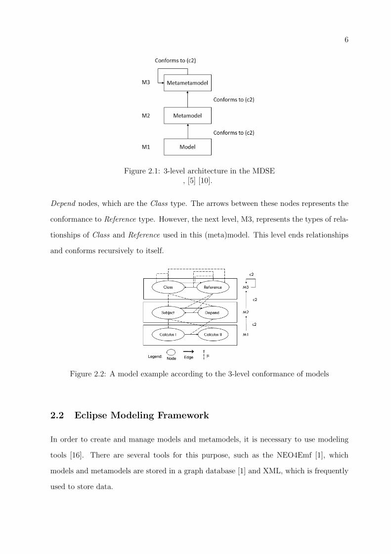
6
Figure 2.1: 3-level architecture in the MDSE, [5] [10].
Depend nodes, which are the Class type. The arrows between these nodes represents the
conformance to Reference type. However, the next level, M3, represents the types of rela-
tionships of Class and Reference used in this (meta)model. This level ends relationships
and conforms recursively to itself.
Figure 2.2: A model example according to the 3-level conformance of models
2.2 Eclipse Modeling Framework
In order to create and manage models and metamodels, it is necessary to use modeling
tools [16]. There are several tools for this purpose, such as the NEO4Emf [1], which
models and metamodels are stored in a graph database [1] and XML, which is frequently
used to store data.

7
The Eclipse Modeling Framework (EMF) 1 enables modeling and generating codes
from model [14]. This framework is used in this dissertation to manipulate models and
metamodels. The EMF uses the ECORE as a metamodel. Its classes are shown in Figure
2.3 and discussed below.
Figure 2.3: Main classes of the Ecore
• EClass: used to model classes [14]. EClass has name and it may have attributes
and references. To support inheritance, one class may refer to many classes of
supertype type [27].
• EAttribute: used to model attributes [14]. It has name and has a data type [27];
• EDatatype: used to represent atomic data [27]. Data types are identified by name
[27];
• EReference: used to model references between a given class [14]. If a bidirectional
association is required, this model can be modeled using two instances of EReference
type, which are connected by opposing references [27] and multiplicities may be
specified. EReference has name.
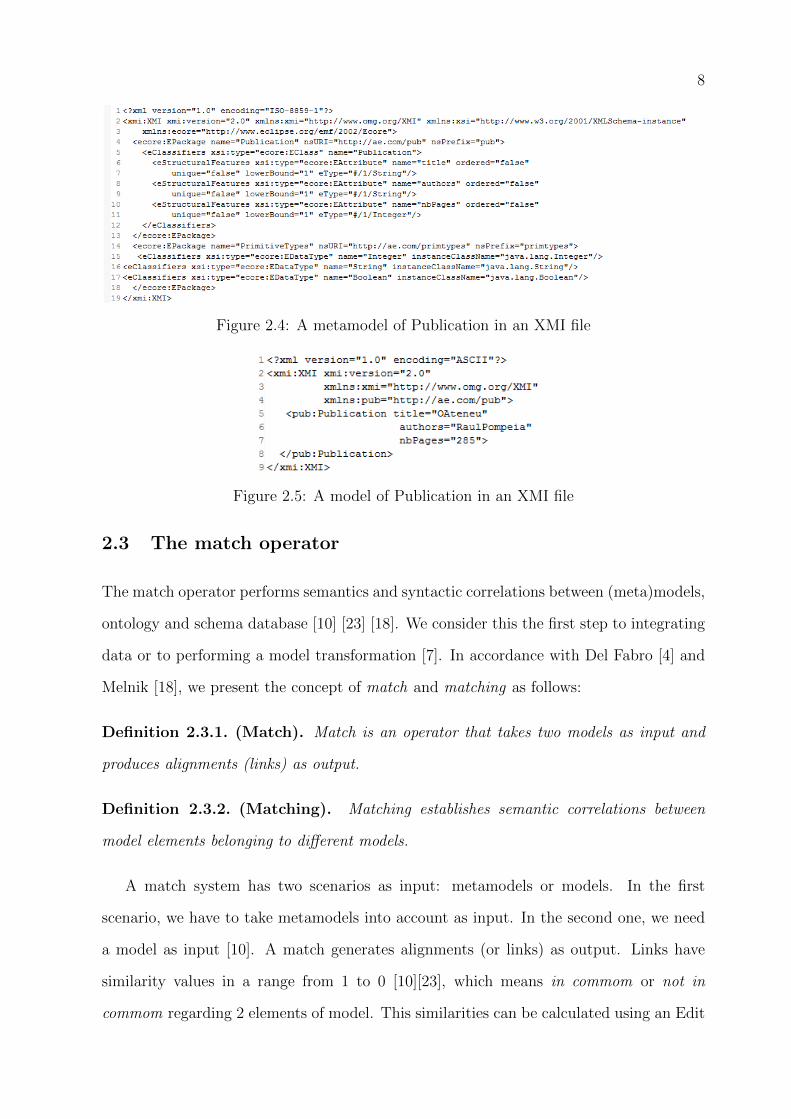
EMF uses XMI (XML Metadata Interchange) to serialize a model and metamodel.
One example of metamodel using XMI is shown in Figure 2.4, which has a title, author
and the number of pages. EPackage groups classes and data of the same types [26]. Figure
2.5 shows the model of the Publication instantiated.
1The Eclipse Modeling Framework is a plug-in for Eclipse and is available athttp://eclipse.org/modeling/emf/
8
Figure 2.4: A metamodel of Publication in an XMI file
Figure 2.5: A model of Publication in an XMI file
2.3 The match operator
The match operator performs semantics and syntactic correlations between (meta)models,
ontology and schema database [10] [23] [18]. We consider this the first step to integrating
data or to performing a model transformation [7]. In accordance with Del Fabro [4] and
Melnik [18], we present the concept of match and matching as follows:
Definition 2.3.1. (Match). Match is an operator that takes two models as input and
produces alignments (links) as output.
Definition 2.3.2. (Matching). Matching establishes semantic correlations between
model elements belonging to different models.
A match system has two scenarios as input: metamodels or models. In the first
scenario, we have to take metamodels into account as input. In the second one, we need
a model as input [10]. A match generates alignments (or links) as output. Links have
similarity values in a range from 1 to 0 [10][23], which means in commom or not in
commom regarding 2 elements of model. This similarities can be calculated using an Edit

9
String Distance, Phonetic Similarity or similarity based on constraints [10] [23]. In the
follow, we present the definition about similarity between 2 strings.
Definition 2.3.3. (Similarity between 2 strings). Given 2 strings: ω1 and ω2, the
similarity between them corresponds to a value indicating how equivalent ω1 is to ω2.
We illustrate the matching of two models in Figure 2.6: Book and Publication. The
links represent the correspondence between two elements [5], and they are assigned with a
similarity value, for example, the link between ”title x title” is 1. This value is calculated
using the Levenshtein Edit Distance and it is normalized in relation to the all links. In
Figure 2.6, the class Book matches to the class Publication and the same situation occurs
with the elements of these classes.
A filter may be applied to select the best links. The most used filter tecnhique is to
set up a minimun treshold value and, then, the links that have the similarity value higher
than this threshold are returned [5]. Below, we define the filter.
Figure 2.6: Matching example between Book and Publication model
Definition 2.3.4. (Filter). A filter is a method that receives a threshold as input to
select the links with similarities higher than (or equal to) this threshold.
10
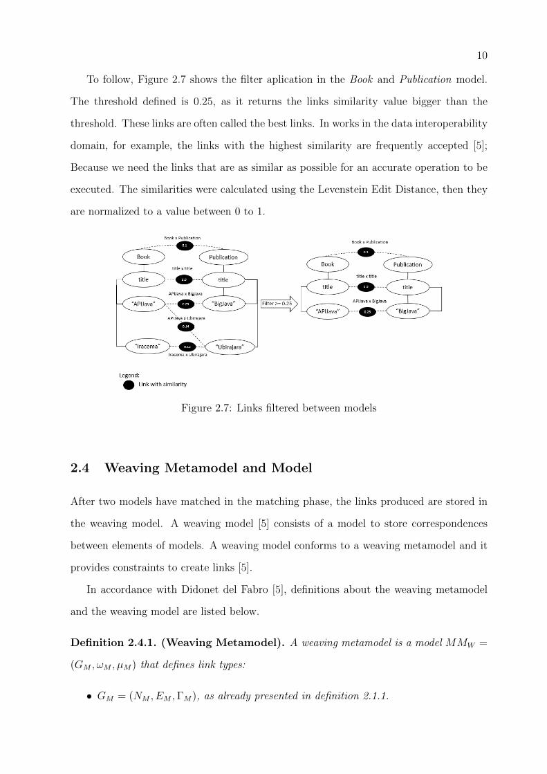
To follow, Figure 2.7 shows the filter aplication in the Book and Publication model.
The threshold defined is 0.25, as it returns the links similarity value bigger than the
threshold. These links are often called the best links. In works in the data interoperability
domain, for example, the links with the highest similarity are frequently accepted [5];
Because we need the links that are as similar as possible for an accurate operation to be
executed. The similarities were calculated using the Levenstein Edit Distance, then they
are normalized to a value between 0 to 1.
Figure 2.7: Links filtered between models
2.4 Weaving Metamodel and Model
After two models have matched in the matching phase, the links produced are stored in
the weaving model. A weaving model [5] consists of a model to store correspondences
between elements of models. A weaving model conforms to a weaving metamodel and it
provides constraints to create links [5].
In accordance with Didonet del Fabro [5], definitions about the weaving metamodel
and the weaving model are listed below.
Definition 2.4.1. (Weaving Metamodel). A weaving metamodel is a model MMW =
(GM , ωM , µM) that defines link types:
• GM = (NM , EM ,ΓM), as already presented in definition 2.1.1.

11
• NM = (NL∪NLE ∪NO), NL is the link type; NLE is the link endpoint type and NO
is the other auxiliary node.
• ΓM : EM −→ (NLXNLE)⋃
(NOXNM) is a link type that refers to multiple link
endpoint types and the auxiliary node refers to any kind of node.
The definition mentioned above is an algebric representation of the weaving meta-
model. However, the elements (core) of weaving metamodel are shown in Figure 2.8. The
core has one link (WLink), and it contains two endpoints (WLinkEnd) - in which the first
endpoint refers to an element in LeftMM, and the second endpoint refers to an element in
RightMM [5]. These links are used for distinct purposes, such as the specification of model
transformations, model traceability or data integration. The elements that compose the
metamodel weaving are listed below:
Figure 2.8: The core of the Metamodel Weaving
• WElement: the main element where all elements inherit [2]. It is composed by the
weaving elements and the reference to corresponded models [5].
• WModel: this represents all model elements [5].
• WLink: this class represents links between model elements [5]. It also refers to
multiple endpoints [2].
• WLinkEnd: this class represents the type of linked elements [2]. It allows the
definition of N-ary links [5].

12
• WElementRef : this class sets an unique ID for a linked element [2].
• WModelRefs: this defines the WLinkEnd and the WElementRef for models as a
whole [2].
Definition 2.4.2. (Weaving Model). A weaving model is a model MW = (GW , ωW , υW ),
a graph GW = (NW , EW ,ΓW ), such that its reference model is a weaving metamodel
(ωW ,MMW ).
Figure 2.9: Conformance to the weaving metamodel, [2]
The composition of 2 different models produce a weaving model: a source metamodel
(LeftMM) and a target metamodel (RightMM) [2] (Figure 2.9). Figure 2.9 shows the
conformance to the model weaving in a generic way. The LeftMM and RightMM conform
to the Weaving Model (WM) and Weaving Metamodel (WMM). The WM conforms to
the WMM, which, in its turns, conforms to the Weaving Metametamodel (WMMM) [5].
The WMMM conforms itself.
The SF [18] attempts to increase the initial similarity and, consequently, better links
are produced. This situation enables the production of better results in operations of the
MDSE (e.g. model transformation). The SF [18] is explained as follows.
2.5 The Similarity Flooding algorithm
The Similarity Flooding algorithm (SF) [18] is a well-known algorithm that propagates
the similarity between model elements in a graph form, which are connected by the same

13
labeled-edge [4] in a fixed-point computation [18]. The SF is frequently used in matching
between metamodels, models, ontologies and data-schemas. For example, consider two
models: A and B. We perform the match between (A x B) in order to establish the
links. The similarities between links may be calculated using an Edit String Distance, as
presented in the previous sections. These values are the initial input for the SF. However,
in an iterative sum, the values between these links are propagated until the minimum
delta value is reached. At the end of this process, the similarities are normalized and
filtered. We explain an example of the SF using real models at the end of this section.
Before executing SF, it is necessary to establish relationships between models elements
to produce a pairwise connectivity graph (PCG). Each node of the PCG is a map pair
-or link [18]. The SF depends on this structure to propagate the similarity values along
the graph, through a propagation graph [18]. The propagation graph goes in opposite
directions in the links: incoming propagation and outgoing propagation [18] [8]. In Figure
2.12 we can see the propagation graphs. Acording to Melnik [18], the propagation graph
is defined below:
Definition 2.5.1. (Propagation Graph). The propagation graph is an auxiliary data
structure that stores the proapgation values (weights) used to propagate the similarities
between links of matched models.
We work with the concept of the restricted propagation graph. The restricted propa-
gation graph propapagates the similarities to an specific kind of link of a matched model,
for example, the propagation only between links of attributes or the propagation only
between links in references. The definition of the restricted propagation graph is given as
follows [5]:
Definition 2.5.2. (Restricted Propagation Graph). The restricted propagation graph
is an auxiliary data structure that stores the propagation values (weights) used to propagate
the similarities between specific links of matched models.
Weights placed in the propagation graph (or in the restricted propagation graph) indi-
cate the propagation coefficient, i.e., how much the similarity of a given link is propagated

14
[18]. Melnik [18] defines 7 ways of calculating the propagation coefficients (π) of the prop-
agation graphs. One of the fix-point formulas proposed by Melnik [18] is calculated over
the inverse-product of the number of links of a matched class. It is used in this dissertation
and shows more accurate results [18] [8].
The similarity propagation may be executed several times, until a given delta is no
longer achieved. The delta is a treshold value previously defined between iterations,
which allows the iteration of the SF to be stopped [18]. This treshold may be defined
if the difference between the similarities regarding iterations is too small, we stop the
execution of the SF. At the end of each iteration of SF, the values are normalized [18].
Finally, the generalized version of SF is σi+1 = targetLinki + (sorceLinki ∗ π), where
the σ relate as a link (alignment), the targetLink and the sourceLink indicate the incoming
and outgoing propagation, respectively, and π indicates the propagation coefficient [18].
We illustrate one execution of the SF as follows. Consider 2 metamodels: Book and
Publication. According to Figure 2.10, the Book metamodel contains the class Book,
which has 1 attribute: title, and 1 reference chapters to class Chapter. The class Chapter
contains the following attributes: title, nbPages, author, book. Class Chapters has one
reference book to class Book. We present the metamodel of Publication in Figure 2.11,
which has 3 attributes: title, authors, nbPages.
Figure 2.10: Book metamodel
Figure 2.11: Publication metamodel
To create the links, we execute a Cartesian Restrict Product. We calculated the
similarities of these links using the Levenshtein Edit Distance [15]. These values initialize

15
Figure 2.12: Partial links between Book and Publication
the SF. The Levenshtein Edit Distance is an algorithm frequently used in academia and
several works. However, we chose this algorithm to illustrated the execution of the SF.
Figure 2.12 provides an overview of the links that were created. As already stated, the
formula for the SF is: σi+1 = targetLinki + (sourceLinki ∗ π); where, targetLink refers
to the links that receive the propagation graph and the sourceLink is the link that the
propagation graph leaves.
Links Initial Similarity π 1st 3rd 6thBook x Publication 0.1 0.16666 0.465 0.466 0.465title x title 1 0.166 0.26 0.12 0.083title x authors 0.142 0.1666 0.040 0.068 0.076chapters x authors 0.1666 0.1666 0.046 0.069 0.076Chapter x Publication 0.09 0.083 1 1 1title x authors 0.142 0.083 0.038 0.072 0.081authors x nbPages 0.125 0.083 0.033 0.070 0.081
Table 2.1: Partial match for Book and Publication
Now we execute the first iteration from the link Book X Publication - sourceLink, to
title X title - targetLink. The iterations are important because they change the similarities
between links. The sourceLink has similarity equal to 0.1, and the targetLink has simi-
larity equal to 1. The propagation coefficient is 0.1666, as we have 6 links in the matched
class, so, 16
= 0.1666. Replacing in the formula, σ1 = 1 + (0.1 ∗ 0.1666), σ1 = 1.01666.
Thus, the new similarity of the link title x title is ∼= 1.01666. We add all the similarity
values that ”arrive” at the link Book x Publication. This produces the new similarity value

16
for the link of the matched class Book X Publication. Table 2.1 shows a partial result
for the matching between Book X Publication, after executing the SF. We stopped the
execution of the SF at the 6th iteration because the delta value was achieved in the links,
valuing ∼= 0.001. At the end of each iteration, the similarity values were normalized.
2.6 Related works
In this section, we explain different ways to encoded the propagation graphs of the SF, in
addition to other algorithms to propagate similarities - beyond what has been proposed
by Melnik [18].
Didonet del Fabro [4] [5] proposes the use of the variants for the propagations in links of
metamodels. This approach allows different ways of propagating similarities considering
structural relationships of different metamodels [4] [10]. The propagations techniques that
were developed are listed below:
• Containment-tree propagation: this allows the propagation of the similarities
from links between classes to links between attributes and/or from links between
classes to links between references [4]. For example, consider two matched classes
and the links between them. This method propagates the similarities between links
of attributes and/or references [4].
• Relationship-tree propagation: this allows the propagation of the similarities to
links of references between classes [4]. Consider two matched classes and the links
between them. This methods only propagates between links of references [4].
• Inheritance-tree propagation: this allows the propagation of the similarities
between links of references with inheritance relationship [4]. For example, this
method extends the Relationship-tree propagation, however, it takes into account
the inheritance of the references [4].
Falleri et al. [8] encoded metamodels into 6 different graph structures in order to
execute the propagations of the SF algorithm. According to Falleri et al. [8], these

17
approaches are more detailed than proposed in Didonet del fabro [4]. The implementations
of the metamodels are:
• Minimal configuration: this requires that we have one labeled node of the graph
created for each EClass [8]. The name of the nodes are the same of the elements,
for example, an element X (an Eclass) with name m is represented by a node N
with label m [8]. According to Falleri et al. [8], this configuration showed the worst
result in the Similarity Flooding, due to its simplicity.
• Basic configuration: A labeled name is linked to a unique identified ID [8].
Thus, it allows frequency of a used given name to be know [8]. This frequency can
be exploited by the SF [8]. For example, an Eclass Ec is presented by a node N
labeled by a unique ID, and linked to a node labeled n with an arc label [8].
• Standard configuration: this obtain the similarities in types and attributes [8].
For example, a node that represents an element x is linked by a labeled node kind
to a node x representing the type of this element [8].
• Full configuration: this extends the Standard configuration as it takes the EAt-
tributes and EReferences into account [8]. For example, all the nodes that represent
an EAttribute or EReference are included an node labeled called derived, giving this
node Boolean conditions (true or false) as to whether the element is derived [8].
• Flattened configuration: this extends the Full configuration, although it deals
with inheritance relationships [8]. For example, the nodes representing supertypes
are deleted from the graph [8]. Thus, it is possible to connect nodes representing
an EClass to nodes representing the EAttributes [8]. When an EReferenceis typed
as an abstract EClass, a node type is created [8].
• Saturated configuration: this extends the Flattened configuration [8]. For ex-
ample, the nodes that represent the EClass are linked in a supertype node [8]. It
represents all the super-classes of this EClass [8]. EClass are also linked in nodes
that represents EAttributes. The node that represents an EReference are created

18
and linked to the node representing the EClass, as well as the nodes representing
the super-class of the EClass [8].
Zhang, Yuan and Huan [32] implemented the SF for the MapReduce. Thus, each
iteractive sum of the Similarity Flooding is a MapReduce job. They applied it in a large-
scale graph datasets. Experimental results show that this implementation can work in
big graph datasets [32].
Truong et al. [29] implemented a new version for SF in the context of integration of
the ontologies. This approach consists of three steps:
1. Ontologies models are encoded into a direct labeled graph [29];
2. The method of concept classification is applied to increase the precision and reduce
the process of the SF [29]. According to Truong et al. [29] this method avoids an
exhaustive comparison of all the nodes of the models;
3. Finally, the Similarity Flooding and a filter are applied [29].
The Uppropagation [7] - which is used in context of database schema and is im-
plemented in Coma++, propagates the similarities in a bottom-up manner, i.e., from
child-nodes to main-nodes [7]. The authors defend the idea that the similarity propa-
gates directly to main-node because the child-nodes have a strong relationship [7]. The
propagated similarity to the main-node is the average of the highest similarity for each
child-nodes [7].
Lily [30] creates alignments between heterogeneous, distributed and large-scale ontolo-
gies. In the matching phase, Lily exploits both linguistic and structural information of
ontology to generate initial alignments [30]. If it is necessary to produce more alignments,
a strategy of similarity propagation is applied [17].
2.6.1 Discussion
We show a comparative table and discuss the propagation techniques presented in sec-
tion 2.6. Table 2.2 summarizes how the propagation of the SF works in the presented

19
approaches. Column approach mentions the author (or the proposed framework); The
Prop. Technique elucidates the technique proposed; The scope shows the field of ap-
plication; and the Similarity Flooding indicates whether the approach is the Similarity
Flooding algorithm or a variant of it.
Del Fabro and Valduriez [4] proposed ways to propagate the link similarity in a meta-
model. The authors proposed a propagation metamodel that is used to propagate the
similarity in metamodels. On the other hand, Falleri et al. [8] proposed 6 strategies to
encode a given metamodel in a graph structure. These methods may provide a better
comprehension of the structure of the metamodel, as the metamodel elements are more
detailed [8]. In the aproach of Del Fabro and Valduriez [4] the lower the quantity of links,
the better the result of the SF, whereas the aproach of Faller et al. [8] may requires a
large amount of elements for the SF to sucess.
Zhang, Yuan and Huan [32] used the MapReduce jobs to iterate the results of the
SF. Truong et al. [29] presented a new version for the Similarity Flooding algorithm, in
which they used the ”classification concepts”, thereby avoiding the exhaustive matching
between elements in ontologies [29].
Other similarity propagation techniques, showing the close of the SF, have also been
studied by researchers. Uppropagation [7], which is used in schema matching, attempts
to minimize the maximum possible loss of similarities when executing the propagations,
using the average of the highest similarity for each element [7]. The propagation is the
type of bottom-up, i.e., from a child-node to a main-node of a given schema model, in a
graph representation. Lily [30], applied to ontologies, uses a decision-maker in order to
perform the propagation of similarity, i.e., if there are few alignments, the similarities are
then propagated to obtain more alignments [30].
We note most of these implementations have a common goal: to attempt to produce
the best alignments to integrate data or process models, and also to explore various
elements present in the formalism in order to perform the best propagation of similarities
[4] [8] [29] [7] [30] [18] [10]. To follow, we positioned our approach in comparison with the
solutions mentioned above, reporting on the main differences between implementations:

20
1. Melnik [18] proposes the SF. However, we create restricted propagation graphs for
this algorithm. Therefore, we can verify whether it is suitable to execute the SF in
a lesser amount of links;
2. As in Didonet del Fabro [4] [5], we create restricted propagation graphs in order
to execute the SF. However, we developed the propagation less generically, i.e.,
involving less elements as possbile. This granularity allows us to compare how the
propagation technique may be advantageous for the SF;
3. Falleri et al. [8] indicated 6 ways to encode a metamodel in a graph structure,
then, the SF is applyed. Unlike this approach, we considered one graph codification
regarding a metamodel (or model) and 9 restricted propagation graphs to execute
the SF;
4. Compared to Zhang, Yuan and Huan [32] and Coma++ [7], our approach deals with
instances of a given model;
5. Unlike Truong et al. [29], we do not consider the use of ”concept of classification”.
However, we apply a filter that returns the best links. This may avoid a repetitive
matching task between metamodels and models;
6. Unlike Lily [30], we do not consider the use of a propagation method to create
more links. Our approach attempts to increase the similarities between the links of
metamodels and models.
According to our knowledge, these are between the most representative approaches
in its field of study. Whereas they all have propagation similarities, it is difficult to
compare them, because the scenarios, the model encodings and the propagation techniques
have differences on the conceptual design and implementation. We gathered some simple
techniques and provide a comparison.

21
Approach / Author Prop. Technique Scope SimilarityFlooding
Del Fabro andValduriez [4]
This takes into account se-mantic and structural informa-tion of a metamodel. Thetechnique may require a smallnumber of elements for a bet-ter performance of the SF.
MDSE X
Falleri et al. [8] Encoded a metamodel in 6graph manners: minimal, ba-sic, standard, full, flattenede satured. The configurationwith more elements providesthe best results for the SF.
MDSE X
Zhang, Yuanand Huan [32]
The algorithm is encondedinto a MapReduce environ-ment. Each job of theMapreduce is a new itera-tive sum of the algorithm.
Data Schema X
Truong et al. [29] This consists of applyinga concept of classificationto increase precision andtry to reduce the process-ment time of the algorithm.
Ontology X
UpPropagation [7] This is used in propagatinginstances of scheme data.The algorithm propagatesthe average of the highestsimilarity values of the in-stances to the attributes.
Data schema
Lily [30] If the first step does notproduce sufficient align-ments, a similarity propa-gation strategy is appliedto obtain more alignments.
Ontology
Table 2.2: Propagation approaches

22
CHAPTER 3
METAMODEL-BASED SIMILARITY PROPAGATION
In this chapter 1, we present and discuss different ways to implement the propagation
methods of the SF. In section 3.1, the methodology workflow of this work is given, in
which the steps are sufficiently detailed to permit reproduction and enable a comparison
with other propagation approaches. Following this, in section 3.2, we explain nine distinct
ways of encoding the SF. For these codification, as already stated, we use information on
the structures of metamodels and models to develop of the propagation methods. This
could permit a reduction in the amount of links and number iterations of the SF in a
single link, which increases the similarity of this related link in as litte iteration possible.
In section 3.3, we present the metamodels and models used to execute the propagation
methods. However, in subsection 3.3.3, we compare of how much these similarities have
been increased (or reduce) in comparison with an implementation comprising all the
propagation methods, which is more similar (though not equivalent) to the original SF
implementation.
3.1 Methodology workflow
The methodology employed in this work is organized in accordance with to Figure 3.1
and may be outlined as follows:
1. Loading metamodels: we load pairs of models with their respective metamodels;
2. Matching: we execute the matching aiming for the creation of the links between
the metamodels and models loaded in step 1. Our motivation is focused on the
match operator, because it is the way to create links in a semi-automatic way. In
addition to the match, there are several operations for establishing links, such as,
1This chapter was partially published in the proceedings of the XVIII Ibero-American Conference onSoftware Engineering, 2015 [21]

23
diff, copy or merge [18] [5]. However, we use the match operator because it returns
the alignments (links) between 2 models [18] [5];
3. Links creation: the links between (meta)models are established. Therefore, sim-
ilarities can be assigned to them. These links can be stored in a weaving model to
serve as input for the next steps [4];
4. Calculating the similarities: we calculate the similarities between links. There
are various ways to calculate their similarities, such as using a String Edit Distance
[23] [18]. In our work, we use a String Edit Distance, which provides the best
sequence of edit operations to convert a string from x to y [31]. As edit operations,
we can outline insertion, deletion and substitution [31]. There are several Edit
Distance functions, e.g., Hamming Distances [11], Longest Commom Subsequence
[20], Smith-Waterman distance [25], Jaro-Winkler distance [31] or Stringsim function
[28]. To calculate the similarities between links, we use a well-know String Edit
Distance called the Levenshtein Edit Distance [15]. The values returned are the
initial input values for the SF. We do not consider the similarities between synonyms.
In this way, a dictionary should be implemented.
5. Link with similarity: the links are assigned to their respective similarity values.
Thus, we can begin the propagation methods, which are explained below;
6. Executing the propagation methods of SF: the methods of the propagation
are executed. We divided these executions into 2 groups according to the config-
uration of two filters. A filter only selects links with a similarity higher than a
given value. According to Melnik [18], SF has a good performance when dealing
with a fewer elements. Therefore, each filter configuration enables a reduction in
the number of processed links. The filter settings can be described as follows. In
the (I) first filter configuration, a filter is applied after running SF. This technique
is related to the works of Falleri et al. [8], Del Fabro [4] and Melnik [18]. In the
(II) second filter configuration, a filter is applied before the SF run. This allows
the propagation methods to be applied to the fewest possible links and, thus, this

24
may increase the similarities in a fewest iterations of the SF due to the smallest
number of links in a matched class. However, this implies that a good threshold
value should be chosen. At the end, we compared to what extent the similarity of
these elements has increased, taking into account the propagation methods used:
restricted propagations X comprising all the propagations methods.
7. Storage in a weaving model: the links are stored in a weaving model. In this
dissertation, the weaving model is persisted in the memory.
Figure 3.1: Methodology workflow
3.2 Implemented methods
We developed 9 ways of execute the restricted propagation according to the structural
information of elements of a given (meta)model: classes, attributes, references, instances
of attributes and the type of these elements (links between String or Integer). These
methods change the direction of the propagation graphs. Then, it is created restriction on
the propagation graphs. We implement the methods in Java language and the metamodels
and the EMF is used to handle the metamodels and models.
We choose these methods because the links are created by matching the elements of
a model and a metamodel as much as possible; giving a representative number of the
links to be compared. This situation enables a comparison of the results at the end.
Furthermore, we can verify if the restricted propagation graphs are viable in comparison

25
to the non-restricted approach. Note that the propagation methods are restricted to a
given type of element and, therefore, cannot be used in any situation.
Figure 3.2: Propagation from links between Classes to links between Attributes
• Propagation from links between Classes to links between Attributes: this
propagates the similarities from links between Classes to links between Attribute
belonging to the same matched classes (Figure 3.2). The propagation is calculated
as: π = 1/Lx, where Lx indicates the number of links between attributes belonging
to Class A and Class B matched, with Lx 6= 0. For example, considering 2 matched
metamodels, this method propagates the similarities from links between classes to
only links of attributes.
Figure 3.3: Propagation from links between Classes to links between References
• Propagation from links between Classes to links between References: this
propagates the similarities from links between classes to links between references
belonging to the same matched classes (Figure 3.3). This is very similar to the

26
previous propagation method but, in this related propagation, links between ref-
erences are considered. The propagation is calculated as: π = 1/Ly, where Ly is
the number of links between references of Class A and Class B matched, with Ly
6= 0. For example, considering 2 matched metamodels, this method propagates the
similarities from links between classes to only links of references.
Figure 3.4: Propagation from links between Classes to links between Attributes andReferences
• Propagation from links between Classes to links between Attributes and
References: this propagates the similarities from links between Classes to links
between Attributes and References belonging to the matched class (Figure 3.4).
The formula of the propagation is: π = 1/Lxy, where Lxy is the amount of the
links between attributes and references of Class A and Class B matched, with
Lxy 6= 0. For example, considering 2 matched metamodels, this method propagates
the similarities from links between classes to only links of attributes and references.
• Propagation from links between Classes to links between References and
Attributes: this propagates the similarities from links between Classes to links
between References matched with Attributes of the same class (Figure 3.5). It
changes the propagation direction in comparison with the previous method. The
propagation is π = 1/Lyx, where Lyx is the amount of links between references
regarding Class A and Class B matched, with Lyx 6= 0. For example, considering
2 matched metamodels, this method propagates the similarities from links between
classes to only links of references and attributes.

27
Figure 3.5: Propagation from links between Classes to links between References andAttributes
• Propagation from links between Attributes to links between their In-
stances: the similarities between links of attributes are propagated to links of their
respective instances (Figure 3.6). The propagation is π = 1/Lι, where Lι desig-
nates the amount of instances of a given attributes regarding Class A and Class B
matched, with Lι 6= 0. For example, considering 2 matched models, this method
propagates the similarities only in links of attributes to links of their instances.
Figure 3.6: Propagation from links between Attributes to links between their Instances
The propagation between links of type belonging of a link are considerate, e.g. Integer,
String or Float. In this case, the similarity of the link between classes is propagated to
the link between types. The methods are detailed as follows:
• Propagation from links between Classes to links between types of the
Attributes: this propagates the similarities from links between Classes to links
between types of the Attributes (Figure 3.7). The propagation is calculated as:

28
π = 1/Ltypex , where Ltypex indicates the number of links between types belonging
to Attribute A and Attribute B matched, with Ltypex 6= 0. For example, considering
2 matched metamodels, this method propagates the similarities from links between
classes to only links of types of attribute.
Figure 3.7: Propagation from links between Classes to links between types of the At-tributes
• Propagation from links between Classes to links between types of the
References: this propagates the similarities from links between Classes to links
between types of the References (Figure 3.8). The propagation is calculated as:
π = 1/Ltypey , where Ltypey indicates the number of links between a type belonging
to Reference A and Reference B matched, with Ltypey 6= 0. For example, considering
2 matched metamodels, this method propagates the similarities from links between
classes to only links of types of references.
• Propagation from links between Classes to links between types of the
Attributes and links between types of the References: this propagates the
similarities from links between Classes to links between types of Attributes and Ref-
erences (Figure 3.9). The propagation is calculated as: π = 1/Ltypexy, where Ltypexy
indicates the number of links between types belonging to Attribute A and Reference
B matched, with Ltypexy 6= 0. For example, considering 2 matched metamodels, this
method propagates the similarities from links between classes to only links of types
of attribute and types of references.

29
Figure 3.8: Propagation from links between Classes to links between types of the Refer-ences
Figure 3.9: Propagation from links between Classes to links between types of the At-tributes and links between types of the References
• Propagation from links between Classes to links between types of the
References and links between types of the Attributes: this propagates the
similarities from links between Classes to link between types belonging to References
and Attributes (Figure 3.10). The propagation is calculated as: π = 1/Ltypeyx,
where Ltypeyx indicates the number of links between types belonging to Reference
A and Attribute B matched, with Ltypeyx 6= 0. For example, considering 2 matched
metamodels, this method propagates the similarities from links between classes to
only links of types of references and types of attributes.
3.3 Case study
In this section, we present 2 case studies involving the methods of the propagation. The
(meta)models were chosen because they are frequently used in academia [18] [5].

30
Figure 3.10: Propagation from links between Classes to links between types of the Refer-ences and links between types of the Attributes
The first case study is related to the matching between partial (meta)models of the
Mantis and Bugzilla. Mantis is a web-based bug-tracking system; Bugzilla serves the same
purpose, although new modules can be added on it [5]. The objective of this matching
is to illustrate the possibility of creating weaving models to integrate 2 different kinds of
software. This practice is important when companies need to integrate their software or
data [5]. This study is outlined in subsection 3.3.1.
In the second case study, we present the matching between two partial (meta)models:
AccountOwner and Customer. These are used in electronic documents for e-business
[18]. The objective of this matching is the same as given in sub-subsection 3.3.1: to
produce a weaving model to integrate both (meta)models. We have outlined this study
in sub-subsection 3.3.2.
3.3.1 Propagation between Mantis and Bugzilla
We have outlined the (meta)models as follows 2. The Mantis' metamodel has 9 classes, 15
attributes and 10 references. The main classes of Mantis are shown in Figure 3.11. The
Bugzilla's metamodel has 9 classes, 39 attributes and 8 references and the main classes
of it are available in Figure 3.12.
According to Table 3.1, the amount of links generated in the matching of these meta-
models and models is shown. We also indicate the number of links after the filter applica-
2The metamodels of Mantis and Bugzilla are available at http://www.emn.fr/z-info/atlanmod/index.php/Ecore

31
Figure 3.11: Main classes of Mantis metamodel
tion, which the threshold is 0.5. We selected this threshold because it returned the best
links according to the calculus of the Levenshtein Edit Distance, after some executions of
the SF. If another technique of the calculus of the similarity is applied, another threshold
should be defined.
Links Matched Amount of Links Generated Amount of Links FilteredLinks between classes 81 11Links between attributes 585 21Links between references 80 2Links between attributes and references 46,800 2Links between references and attributes 46,800 10Links between types of attributes 585 21Links between types of references 80 2Links between types of attributesand references
46800 2
Links between types of referencesand attributes
80 10
Table 3.1: Amount of links generated in the matching phase: Mantis and Bugzilla
Whereas an instance is explicitly related to a class, we make a distinction between
the model elements representing a class (called a class instance) and the model elements
representing the values of the attributes (called an attribute instance). The Mantis' model
has 5 classes instances, 12 attributes with 1 attribute for each instance. The Bugzilla's
model has 4 instances of a classes and 31 attributes instances with 1 attribute per instance.
According to Table 3.2, the matching generated:

32
Figure 3.12: Main classes of Bugzilla Metamodel
Links Matched Amount of Links Generated Amount of Links FilteredLinks between instances of attributes 372 22
Table 3.2: Amount of links of instances generated in the matching phase: Mantis andBugzilla
Table 3.3 and 3.4 show the results according to each propagation method and in
Table 3.5 shows the results comprising all the propagation methods. Table 3.6 shows
the propagation values according to the type of a given element and Table 3.7 shows
the propagation comprising all the methods regarding the type of link. All the tables
display the results of the (I) first filter and (II) filter configurations; π indicates the
propagation coefficient; the link with (∗) represents the links between classes or links
between attributes. The settings of iterations for the Similarity Flooding are 1, 3 and 6.
The value of the π differs for the number of links according to the filter configuration.
For example, the link of the class IdentifiedElt x LongDesc has 4 links in the first filter
configuration; thus, π = 1/Lx = 14
= 0.25. On the other hand, the same link, in the second
filter configuration, has 1 link to execute the propagation; thus, π = 1/Lx = 11
= 1. This

33
logic ensues for all other links of model elements.
3.3.2 Propagation between AccountOwner and Customer
To follow, we present the elements of AccountOwner and Customer [18]. The Accoun-
tOwner's metamodel (Figure 3.13) has 2 classes, 7 attributes and 2 references. The
Costumer's metamodel (Figure 3.14) has 2 classes, 5 attributes and 2 references. Accord-
ing to Table 3.8, the matching between both metamodels is shown. We also indicate the
number of the links after the filter application, which the threshold is 0.25. We selected
this threshold because it returned the best links according to the calculus of the Leven-
shtein Edit Distance, after some executions of the SF. If another technique of the calculus
of the similarity is applied, another threshold should be defined.
Figure 3.13: AccountOwner Metamodel
Figure 3.14: Customer Metamodel
In the model of AccountOnwer, we have 2 instances of classes and 7 instances of
attributes. In the model of Customer, we have 2 instances of classes and 5 instances of
attributes. Table 3.9 shows the amount of links generated in the match phase. In this
case, due to a limited number of elements, we do not use filters in the propagation.
Table 3.10 shows the results of restricted propagation between links of AccountOwner
x Customer, according to the specific filter configuration. We set the threshold for the
filter valuing 0.125. The propagation executing all the methods are shown in Table 3.11.
The restricted propagation results between types of links are shown in Table 3.12 and the

34
propagation involving all the propagation methods is shown in Table 3.13.
3.3.3 Discussion
We implemented 9 restricted propagation graphs between structures based on the meta-
model and model elements to propagate similarities between their links. In addition, we
execute these propagations using two different filter configurations: after and before the
execution of the SF (as illustrated in Figure 3.1).
We use 4 sets of metamodels in our experiments: Mantis x Bugzilla and AccountOwner
x Customer. The methods and (meta)models are rather simple, but executing them
enables some conclusions to be drawn regarding the propagation of similarity process. In
the following case, we compared the restricted methods with a combined propagation.
The combined propagation executes all the propagation methods together (non-restricted
propagation). This method show close as proposed in Melnik [18].
We summarize the percentage of the gain of the similarities for the metamodels of
Mantis x Bugzilla and AccountOwner x Customer in Table 3.14 and Table 3.15, respec-
tively. We compare the mean of the similarities of each restricted propagation graph with
the non-restricted propagation. Therefore, the higher the similarity percentage, the better
the restricted propagation technique is in relation to non-restricted propagation.
We discuss the results of the propagation between links of Mantis x Bugzilla. Table
3.14 provides a big picture of the results of each propagation methods compared with
a combined propagation method. This table shows the mean percentage gain over the
iteration of the SF in accordance to the results of (I) filter configuration and (II) filter
configuration. The best implementation for the SF are related to the propagation from
links between Classes to links between References and propagation from links between
Classes to links between types of References in the 6th iteration of (I) filter configuration,
and in the 1st iteration of (I) filter configuration, respectively, due to the small number
of the links. While the worst similarities avarege comes from the methods which were
executed in a large number of the links in a matched classes, e.g., propagation from links
between Classes to links between References and Attributes in any iteration of (II) filter

35
configuration and propagation from links between Classes to links between of types of
References and Attributes in the 1st iteration of (II) filter configuration.
According to the AccountOwner x Customer metamodels and models, we have in-
sights, which are disscused below. A summary of the percentage of the mean between
the methods is provided in Table 3.15. The best propagation techique is the propagation
from links between Classes to links between References. The avarege of the similarities
values increased in the 6th iteration of (I) filter configuration. According to the propaga-
tion between the types of the links, the best propagation method is the propagation from
links between Classes to links between types of References. The avarege of the similarities
values increased in the 6th iteration of (I) filter configuration. In these configurations, the
restricted propagation reduced the number of the links and then increased the average of
the similarities. The worst results come from the propagation from links between Classes
to links between Attributes and propagation from links between Classes to links between
types of Attributes, in the 1st iteration of (II) filter configuration and in the 3rd iteration
of (II) filter configuration, respectively, due to the high value of the total number of the
links.
The second filter configuration acted as a constraint, reducing the number of the links.
Therefore, we did not find a significant increase relative to the average of the similarity
in comparison with the combined method, with the average of the similarities remaining
constant for each iteration of the SF. However, by comparing the filter configurations,
regardless of the propagation methods, there is an increase in the similarities between the
links or no change in the similarities in the iterations of the SF.
In both metamodels (Mantis x Bugzilla or AccountOwner x Customer) in the prop-
agation from links between Attributes to links between their Instances, we observed that
the similarities are unable to ’flow’ between links, where the propagation coefficient is
equal to 1. For example, from the link ’version x version’ to the link ’Beta x beta’, the
same similarity of the link of the attribute is equal to the similarity of the link of the
instance, in any iteration (Table 3.14). Due to the reduced number of the links, the (II)
filter configuration has no effect on the iterations.

36
In all metamodels and models, from the 6th iteration, the values of the similarities
between the links began to gradually decrease, when the delta value has a treshold value
of ∼= 0.001. Thus, we stopped the execution of the SF. The SF tends to propagate the
similarity to a class or element that has the highest number of links. For this reason,
after each iteration and normalization of the results, the similarity increased in a single
kind of link, e.g., the link between classes Address x CustomerAddress in the propagation
from links between Classes to links between Attributes or Issue x Bug in the propagation
comprising all the propagation methods. Therefore, similarity values of 1 were assigned
to these elements in every iteration. Due to this behavior of the SF, in some iterations
the similarities between the links were reduced due to these (meta)models being more
connected, e.g., the propagation from links between Classes to links between Attributes in
the 3rd interation of Mantis x Bugzilla. By the best filter technique, it may be possible
to disconnect the (meta)models. Thus, the results will not tend to be concentrated in a
single link. However, it is important to know the nature of the metamodels and models
in order to choose the best propagation method.
Analyzing the formula of the SF we can deduce the behavior of the algorithm in
(meta)models in different situations. The formula returns the final similarity between
links in accordance with the propagation coefficient multiplied by the similarity of the links
between classes, plus the similarity of the links between attributes and/or references, thus
SF = targetLink + (sourceLink * propagationCoefficient). The propagation coefficient is
directly related to the inverse amount of links to a matched class, thus, 1/amountofLinks.
However, the smaller the amount of links, the better the result of the SF may be. This
situation is shown in both (meta)models used. It is also necessary take into account the
similarity value of the sourceLink, because if this value equals 0, the result may be the
targetLink. Nevertheless, if the targetLink is equal to 0, the result of SF may be the
(sourceLink * propagationCoefficient). Consequently, it is necessary to apply the best
filter techniques when the number of the links is unknown to return the links with the
best similarities, which may increase the result of SF. In this work, we know the number
of links prior to the filter application. However, when using large-scale (meta)models, it

37
is recommend that the number of the links of each matched class be reduced, which may
improve their results.
The links and the weaving model are persisted in memory, which could allow the
weaving model to be handled faster than a model stored in a file. The EMF has specific
classes to persist the weaving model in an XMI file. The weaving model was implemented
using Java language.
Our work does not target only MDSE applications. The methods developed may be
used to discover mutual friends in a social network [18] or to unveil cartels in public
bids [9]. The high similarity may indicates a strong friendship between people [18] or may
indicate fraud in public tenders [9], respectively. This will depend on the enconding of the
similarity values, for example, the use of the Edit Distance. The restricted propagation
methods also may be applied to the Geographic Information System, in which it may be
possible to match schemas of maps [22].
The advantage of the use of restricted propagation graphs is that they can be applied
in different metamodels and models [4]. These methods also may reduce the links of a
matched class, thus, enhancing the similarities between the links. A limitation of this
study is that our implementation does not deal with links concerning inheritance prop-
agation. However, it can be inferred that abstract classes with a generic structure (e.g.
an ’Object’ class), would have several links and the similarity of this class would greatly
increase. The way the links were filtered is also a limitation. Del Fabro and Valduriez
[4] show that such an implementation can be a disadvantage, since the limit value for the
filter is known. After analysis, these values returned the links with a best match. The
evaluation of the similarities should be calculated using Precision and Recall to ensure
greater reliability. Finally, we could implement a dictionary, using ontology, in order to
handle with synonyms.
3.4 Summary
In this chapter, we presented the methodology for comparing the executions of the SF.
We compare the average of the similarity of each restricted propagation graph with the

38
propagation executing all the methods (shown as closely as proposed by Melnik [18]). We
utilize 4 metamodels to execute the propagation: matching between Mantis with Bugzilla
and matching between AccountOwner x Customer. The propagation using the restricted
propagation graphs increase the similarities between the links because they reduce the
number of the links of a matched class.
We also apply 2 variants of filters configuration: before and after the execution of the
SF, as in Figure 3.1. The application of the filter before of the SF enables a comparison
if the number of the links of a matched class is diminished, it is possible increase the
similarity between the links. Applying the filter after the SF only selects the links with
the best similarities, and they have no effect on the propagations. According to our
experiments, the choice of the filter configuration increases the similarities between links,
mainly if we execute the filter after the execution of the SF, because this reduces the
number of the links.
Tables 3.14 and 3.15 show the percent of the gain of similarity. The comparison is
the average of the similarities of the restricted graph propagation with the average of the
similarities of the non-restricted propagation. Therefore, the higher the percentage, the
better the similarity improvement of the application of the restricted propagation graphs.
We executed the iterations of the SF until the 50th iteration. However, the results are
showed to be more appropriate up to the 6th iteration, due to the limit of the delta value.
Therefore the similarities between the links has decreased progressively.
The advantage of using the restricted propagation graph is that this method may
increase faster the similarities between the links, in comparison with a non-restricted
propagation. On the other hand, we must know the features of the metamodels and
models before apply the restricted propagation method in order to provide the best result.

39
Linksπ
Similarities1st 3rd 6th
I II I II I II I IIPropagation from links between Classes to links between Attributes
IdentifiedElt x LongDesc* 0.25 1 0.091 0.047 0.195 0.047 0.195 0.047 0.195id x who 0.25 1 0.250 0.019 0.195 0.014 0.195 0.012 0.195IdentifiedElt x Attachment* 0.125 1 0.091 0.154 0.623 0.154 0.623 0.154 0.624id x id 0.125 1 1.000 0.070 0.623 0.032 0.623 0.021 0.624Issue x BugzillaRoot* 0.04166 1 0.083 0.244 0.619 0.244 0.619 0.244 0.619version x version 0.04166 1 1.000 0.069 0.619 0.025 0.619 0.012 0.619Issue x Bug* 0.007575 1 0.200 1.000 0.686 1.000 0.686 1.000 0.686version x version 0.007575 1 1.000 0.069 0.686 0.023 0.686 0.009 0.686ValueWithId x StringElt* 1 1 0.083 0.074 0.619 0.074 0.619 0.074 0.617value x value 1 1 1.000 0.074 0.619 0.074 0.619 0.074 0.619ValueWithId x Attachment* 0.125 1 0.091 0.100 0.195 0.100 0.195 0.100 0.195value x date 0.125 1 0.250 0.018 0.195 0.014 0.195 0.013 0.195Note x LongDesc* 0.25 1 0.143 0.056 0.225 0.056 0.225 0.056 0.225text x thetext 0.25 1 0.250 0.020 0.225 0.015 0.225 0.014 0.225Note x Attachment* 0.125 0.5 0.111 0.108 0.349 0.108 0.349 0.108 0.349text x desc 0.125 0.5 0.250 0.018 0.175 0.014 0.175 0.014 0.175text x type 0.125 0.5 0.25 0.018 0.175 0.015 0.174 0.014 0.175Attachment x Attachment* 0.03125 0.333 1 0.348 1.000 0.348 1.000 0.348 1.000size x id 0.03125 0.333 0.25 0.019 0.333 0.013 0.333 0.011 0.333size x date 0.03125 0.333 0.25 0.019 0.333 0.013 0.333 0.011 0.333size x type 0.03125 0.333 0.25 0.019 0.333 0.013 0.333 0.011 0.333
Propagation from links between Classes to links between ReferencesIssue x Bug* 0.0142857 1 0.2 1.000 1.000 1.000 1.000 1.000 1.000attachments attachment 0.0142857 1 0.5 0.065 1.000 0.027 1.000 0.016 1.000
Propagation from links between Classes to links between Attributes and ReferencesIdentifiedElt x Bug* 0.142857 1 0.071 0.243 1 0.243 1.000 0.243 1.000id cc 0.142857 1 0.333 0.080 1 0.046 1.000 0.036 1.000
Propagation from links between Classes to links between References and AttributesIssue x Bug* 0.0045 0.25 0.2 1.000 1.000 1.000 1.000 1.000 1.000project x product 0.0045 0.25 0.333 0.013 0.162 0.007 0.228 0.005 0.247priority x priority 0.0045 0.25 1 0.039 0.444 0.013 0.298 0.006 0.256reporter x exporter 0.0045 0.25 0.333 0.013 0.162 0.007 0.228 0.005 0.247assignedTo x assigned To 0.0045 0.25 0.5 0.019 0.232 0.008 0.246 0.005 0.249Issue x BugzillaRoot* 0.025 1 0.0833 0.183 0.176 0.183 0.176 0.183 0.176reporter x exporter 0.025 1 0.333 0.013 0.176 0.007 0.176 0.005 0.176Issue x Attachment 0.0125 1 0.1 0.373 0.148 0.373 0.148 0.373 0.148notes x date 0.0125 1 0.25 0.010 0.148 0.006 0.148 0.005 0.148
Propagation from links between Attributes to links between Instancesversion x version * 1 - 1 1 - 1.000 - 1.000 -Beta x beta 1 - 1 1 - 1.000 - 1.000 -category x exporter * 1 - 0.111 0.180 - 0.181 - 0.181 -website x teste 1 - 0.25 0.180 - 0.181 - 0.181 -category x product* 1 - 0.111 0.555 - 0.556 - 0.556 -website x website 1 - 1 0.555 - 0.556 - 0.556 -version x exporter* 1 - 0.111 0.180 - 0.181 - 0.181 -Beta x teste 1 - 0.25 0.180 - 0.181 - 0.181 -version x version * 1 - 1 1 - 1.000 - 1.000 -Beta x beta 1 - 1 1 - 1.000 - 1.000 -value x component * 1 - 0.111 0.180 - 0.181 - 0.181 -High x link 1 - 0.25 0.180 - 0.181 - 0.181 -value x value * 1 - 1 0.625 - 0.625 - 0.625 -High x link 1 - 0.25 0.625 - 0.625 - 0.625 -
Table 3.3: Propagations from links between Mantis and Bugzilla metamodels and models

40
Linksπ
Similarities1st 3rd 6th
I II I II I II I IIPropagation from links between Attributes to links between their Instancesvalue x exporter * 1 - 0.125 0.1875 - 0.188 - 0.188 -low x abc 1 - 0.25 0.1925 - 0.188 - 0.188 -value x bug id * 1 - 0.143 0.196 - 0.196 - 0.196 -low x 1 1 - 0.25 0.196 - 0.196 - 0.196 -value x component * 1 - 0.111 0.180 - 0.181 - 0.181 -low x link 1 - 0.25 0.180 - 0.181 - 0.181 -value x target milestone * 1 - 0.0714 0.160 - 0.161 - 0.161 -low x v01 1 - 0.25 0.160 - 0.161 - 0.161 -value x bug severity * 1 - 0.083 0.541 - 0.542 - 0.542 -low x low 1 - 1 0.541 - 0.542 - 0.542 -value x value * 1 - 1 0.625 - 0.625 - 0.625 -low x link 1 - 0.25 0.625 - 0.625 - 0.625 -login x version* 1 - 0.1667 0.208 - 0.208 - 0.208 -geor x beta 1 - 0.25 0.208 - 0.208 - 0.208 -value x assigned to* 1 - 0.0909 0.212 - 0.212 - 0.212 -George x Jorge 1 - 0.333 0.212 - 0.212 - 0.212 -login x version* 1 - 0.1667 0.208 - 0.208 - 0.208 -geor x beta 1 - 0.25 0.208 - 0.208 - 0.208 -login x bug severity* 1 - 0.0909 0.170 - 0.170 - 0.170 -geor x low 1 - 0.25 0.170 - 0.170 - 0.170 -value x bug status* 1 - 0.111 0.180 - 0.181 - 0.181 -null x st null 1 - 0.25 0.180 - 0.181 - 0.181 -login x version* 1 - 0.1667 0.208 - 0.208 - 0.208 -geor x beta 1 - 0.25 0.208 - 0.208 - 0.208 -value x assigned to* 1 - 0.0909 0.212 - 0.212 - 0.212 -George x Jorge 1 - 0.333 0.212 - 0.212 - 0.212 -login x version* 1 - 0.167 0.208 - 0.208 - 0.208 -geor x beta 1 - 0.25 0.208 - 0.208 - 0.208 -login x bug severity* 1 - 0.0909 0.170 - 0.170 - 0.170 -geor x low 1 - 0.25 0.170 - 0.170 - 0.170 -
Table 3.4: Continuation - Propagation results from links between Mantis and Bugzillametamodels and models
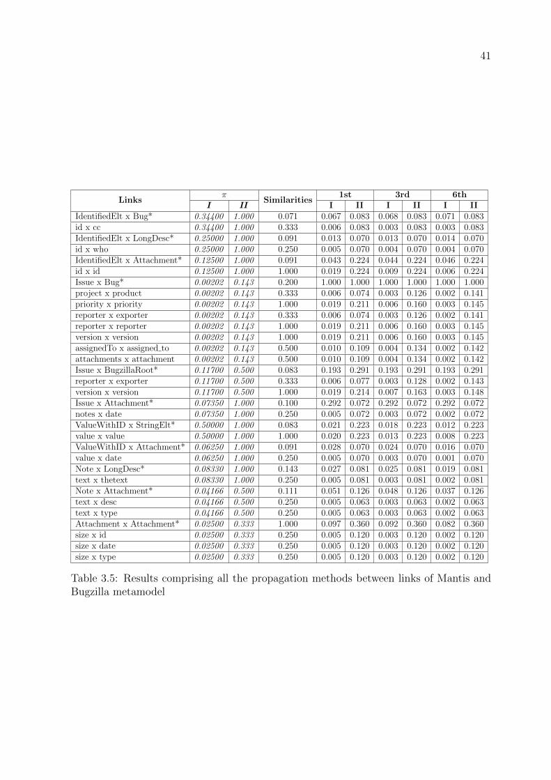
41
Linksπ
Similarities1st 3rd 6th
I II I II I II I IIIdentifiedElt x Bug* 0.34400 1.000 0.071 0.067 0.083 0.068 0.083 0.071 0.083id x cc 0.34400 1.000 0.333 0.006 0.083 0.003 0.083 0.003 0.083IdentifiedElt x LongDesc* 0.25000 1.000 0.091 0.013 0.070 0.013 0.070 0.014 0.070id x who 0.25000 1.000 0.250 0.005 0.070 0.004 0.070 0.004 0.070IdentifiedElt x Attachment* 0.12500 1.000 0.091 0.043 0.224 0.044 0.224 0.046 0.224id x id 0.12500 1.000 1.000 0.019 0.224 0.009 0.224 0.006 0.224Issue x Bug* 0.00202 0.143 0.200 1.000 1.000 1.000 1.000 1.000 1.000project x product 0.00202 0.143 0.333 0.006 0.074 0.003 0.126 0.002 0.141priority x priority 0.00202 0.143 1.000 0.019 0.211 0.006 0.160 0.003 0.145reporter x exporter 0.00202 0.143 0.333 0.006 0.074 0.003 0.126 0.002 0.141reporter x reporter 0.00202 0.143 1.000 0.019 0.211 0.006 0.160 0.003 0.145version x version 0.00202 0.143 1.000 0.019 0.211 0.006 0.160 0.003 0.145assignedTo x assigned to 0.00202 0.143 0.500 0.010 0.109 0.004 0.134 0.002 0.142attachments x attachment 0.00202 0.143 0.500 0.010 0.109 0.004 0.134 0.002 0.142Issue x BugzillaRoot* 0.11700 0.500 0.083 0.193 0.291 0.193 0.291 0.193 0.291reporter x exporter 0.11700 0.500 0.333 0.006 0.077 0.003 0.128 0.002 0.143version x version 0.11700 0.500 1.000 0.019 0.214 0.007 0.163 0.003 0.148Issue x Attachment* 0.07350 1.000 0.100 0.292 0.072 0.292 0.072 0.292 0.072notes x date 0.07350 1.000 0.250 0.005 0.072 0.003 0.072 0.002 0.072ValueWithID x StringElt* 0.50000 1.000 0.083 0.021 0.223 0.018 0.223 0.012 0.223value x value 0.50000 1.000 1.000 0.020 0.223 0.013 0.223 0.008 0.223ValueWithID x Attachment* 0.06250 1.000 0.091 0.028 0.070 0.024 0.070 0.016 0.070value x date 0.06250 1.000 0.250 0.005 0.070 0.003 0.070 0.001 0.070Note x LongDesc* 0.08330 1.000 0.143 0.027 0.081 0.025 0.081 0.019 0.081text x thetext 0.08330 1.000 0.250 0.005 0.081 0.003 0.081 0.002 0.081Note x Attachment* 0.04166 0.500 0.111 0.051 0.126 0.048 0.126 0.037 0.126text x desc 0.04166 0.500 0.250 0.005 0.063 0.003 0.063 0.002 0.063text x type 0.04166 0.500 0.250 0.005 0.063 0.003 0.063 0.002 0.063Attachment x Attachment* 0.02500 0.333 1.000 0.097 0.360 0.092 0.360 0.082 0.360size x id 0.02500 0.333 0.250 0.005 0.120 0.003 0.120 0.002 0.120size x date 0.02500 0.333 0.250 0.005 0.120 0.003 0.120 0.002 0.120size x type 0.02500 0.333 0.250 0.005 0.120 0.003 0.120 0.002 0.120
Table 3.5: Results comprising all the propagation methods between links of Mantis andBugzilla metamodel

42
Links Type link elementπ
Similarities1st 3rd 6th
I II I II I II I IIFrom links between Classes to links between types of Attributes
IdentifiedElt x LongDesc* - 0.250 1.000 0.091 0.007 0.111 0.007 0.111 0.007 0.111id x who Integer x String 0.250 1.000 0.143 0.002 0.111 0.002 0.111 0.002 0.111IdentifiedElt x Attachment* - 0.125 1.000 0.091 0.012 0.111 0.012 0.111 0.012 0.111id x id Integer x String 0.125 1.000 0.143 0.002 0.111 0.002 0.111 0.002 0.111Issue x BugzillaRoot* - 0.042 1.000 0.083 0.182 0.513 0.182 0.513 0.182 0.513version x version String x String 0.042 1.000 1.000 0.011 0.513 0.008 0.513 0.008 0.513Issue x Bug* - 0.008 1.000 0.200 1.000 0.569 1.000 0.568 1.000 0.568version x version String x String 0.008 1.000 1.000 0.011 0.569 0.008 0.568 0.008 0.568ValueWithId x StringElt* - 1.000 1.000 0.083 0.011 0.513 0.011 0.513 0.011 0.513value x value String x String 1.000 1.000 1.000 0.011 0.513 0.011 0.513 0.011 0.513ValueWithId x Attachment* - 0.125 1.000 0.091 0.058 0.513 0.058 0.517 0.058 0.517value x date String x String 0.125 1.000 1.000 0.011 0.513 0.008 0.517 0.007 0.517Note x LongDesc* - 0.250 1.000 0.143 0.044 0.542 0.044 0.541 0.044 0.541text x thetext String x String 0.250 1.000 1.000 0.011 0.542 0.011 0.541 0.011 0.541Note x Attachment* - 0.125 0.500 0.111 0.058 1.000 0.058 1.000 0.058 1.000text x desc String x String 0.125 0.500 1.000 0.011 0.500 0.008 0.500 0.007 0.500text x type String x String 0.125 0.500 1.000 0.011 0.500 0.008 0.500 0.007 0.500Attachment x Attachment* - 0.031 0.333 1.000 0.193 0.677 0.193 0.677 0.193 0.677size x id Integer x String 0.031 0.333 0.143 0.002 0.226 0.005 0.226 0.006 0.226size x date Integer x String 0.031 0.333 0.143 0.002 0.226 0.005 0.226 0.006 0.226size x type Integer x String 0.031 0.333 0.143 0.002 0.226 0.005 0.226 0.006 0.226
From links between Classes to links between types of ReferencesIssue x Bug* - 0.0143 1 0.2 1.000 1.000 1.000 1.000 1.000 1.000attachments attachment Attachment x Attachment 0.0143 1 1 0.120 1.000 0.041 1.000 0.018 1.000
From links between Classes to links between types of Attributes and ReferencesIdentifiedElt x Bug* - 0.143 1 0.071 0.171 1 0.171 1 0.171 1id cc Integer x Cc 0.143 1 0.125 0.027 1 0.025 1 0.025 1
From links between Classes to links between types of References and AttributesIssue x Bug* - 0.0045 0.2 0.200 1.000 1.000 1.000 1.000 1.000 1.000project x product ValueWithId x String 0.0045 0.2 0.091 0.004 0.148 0.004 0.187 0.005 0.198priority x priority ValueWithId x String 0.0045 0.2 0.091 0.004 0.148 0.004 0.187 0.005 0.198reporter x exporter Person x String 0.0045 0.2 0.167 0.007 0.235 0.005 0.209 0.005 0.201reporter x reporter Person x String 0.0045 0.2 0.167 0.007 0.235 0.005 0.209 0.005 0.201assignedTo x assigned To Person x String 0.0045 0.2 0.167 0.007 0.235 0.005 0.209 0.005 0.201Issue x BugzillaRoot* - 0.0250 1 0.083 0.184 0.284 0.184 0.284 0.184 0.284reporter x exporter Person x String 0.0250 1 0.167 0.007 0.284 0.005 0.284 0.005 0.284Issue x Attachment* - 0.0125 1 0.100 0.358 0.276 0.358 0.276 0.292 0.276notes x date Note x String 0.0125 1 0.143 0.006 0.276 0.005 0.276 0.005 0.276
Table 3.6: Results of the propagation between types of links of Mantis and Bugzillametamodels

43
Links Type link elementπ
Similarities1st 3rd 6th
I II I II I II I IIIdentifiedElt x Bug* - 0.0344 1.000 0.071 0.030 0.140 0.031 0.140 0.032 0.140id x cc Integer x Cc 0.0344 1.000 0.333 0.001 0.140 0.001 0.140 0.001 0.140IdentifiedElt x LongDesc* - 0.2500 1.000 0.091 0.005 0.081 0.005 0.081 0.005 0.081id x who Integer x String 0.2500 1.000 0.143 0.001 0.081 0.001 0.081 0.001 0.081IdentifiedElt x Attachment* - 0.1250 1.000 0.091 0.009 0.081 0.009 0.081 0.009 0.081id x id Integer x String 0.1250 1.000 0.143 0.001 0.081 0.001 0.081 0.001 0.081Issue x Bug* - 0.0020 0.143 0.200 1.000 1.000 1.000 1.000 1.000 1.000project x product ValueWithId x String 0.0020 0.143 0.091 0.001 0.069 0.002 0.118 0.002 0.140priority x priority ValueWithId x String 0.0020 0.143 0.091 0.001 0.069 0.002 0.118 0.002 0.140reporter x exporter Person x String 0.0020 0.143 0.167 0.001 0.068 0.002 0.124 0.002 0.141reporter x reporter Person x String 0.0020 0.143 0.167 0.001 0.068 0.002 0.124 0.002 0.141version x version String x String 0.0020 0.143 1.000 0.008 0.357 0.003 0.196 0.002 0.150assignedTo x assigned to Person x String 0.0020 0.143 0.167 0.001 0.068 0.002 0.124 0.002 0.141attachments x attachment Attachment x Attachment 0.0020 0.143 1.000 0.008 0.357 0.003 0.196 0.002 0.150Issue x BugzillaRoot* - 0.0118 0.500 0.083 0.180 0.434 0.180 0.434 0.180 0.434reporter x exporter Person x String 0.0118 0.500 0.167 0.001 0.072 0.002 0.181 0.002 0.212version x version String x String 0.0118 0.500 1.000 0.008 0.361 0.004 0.253 0.002 0.221Issue x Attachment* - 0.0074 1.000 0.100 0.247 0.084 0.247 0.084 0.247 0.084notes x date Note x String 0.0074 1.000 0.143 0.001 0.084 0.002 0.084 0.002 0.084ValueWithID x StringElt* - 0.5000 1.000 0.083 0.008 0.376 0.007 0.376 0.005 0.376value x value String x String 0.5000 1.000 1.000 0.008 0.376 0.005 0.376 0.003 0.376ValueWithID x Attachment* - 0.0625 1.000 0.091 0.041 0.379 0.036 0.379 0.024 0.379value x date String x String 0.0625 1.000 1.000 0.008 0.379 0.004 0.379 0.002 0.379Note x LongDesc* - 0.0833 1.000 0.143 0.036 0.397 0.033 0.397 0.026 0.397text x thetext String x String 0.0833 1.000 1.000 0.008 0.397 0.004 0.397 0.003 0.397Note x Attachment* - 0.0417 0.500 0.111 0.051 0.733 0.047 0.733 0.037 0.624text x desc String x String 0.0417 0.500 1.000 0.008 0.366 0.004 0.366 0.002 0.366text x type String x String 0.0417 0.500 1.000 0.008 0.366 0.004 0.366 0.002 0.366Attachment x Attachment* - 0.1250 0.333 1.000 0.137 0.496 0.131 0.496 0.117 0.496size x id Integer x String 0.1250 0.333 0.143 0.001 0.165 0.003 0.165 0.003 0.165size x date Integer x String 0.1250 0.333 0.143 0.001 0.165 0.003 0.165 0.003 0.165size x type Integer x String 0.1250 0.333 0.143 0.001 0.165 0.003 0.165 0.003 0.165
Table 3.7: Results comprising all the propagation methods between types of links ofMantis and Bugzilla
Links Matched Amount of Links Generated Amount of Links FilteredLinks between classes 2 2Links between attributes 35 25Links between references 4 1Links between attributes with references 14 5Links between references with attributes 10 4Links between types of attributes 35 25Links between types of references 4 1Links between types of attributeswith reference
14 7
Links between types of referenceswith attributes
10 5
Table 3.8: Amount of links generated in the matching phase: AccountOwner and Cus-tomer
Links Matched Amount of Links Generated Amount of Links FilteredLinks between instances of attributes 10 10
Table 3.9: Amount of links of instances generated in the matching phase: AccountOwnerand Customer

44
Linksπ
Similarities1st 3rd 6th
I II I II I II I IIPropagation from links between Classes to links between Attributes
AccountOwner x Customer * 0.333 0.500 0.143 0.203 0.196 0.203 0.196 0.203 0.196name x Cname 0.333 0.500 0.500 0.126 0.146 0.082 0.110 0.069 0.099birthdate x Cname 0.333 0.500 0.125 0.040 0.050 0.061 0.086 0.067 0.096AccountOwner x CustomerAdress* 0.083 0.143 0.071 0.376 0.285 0.376 0.285 0.376 0.285name x street 0.083 0.143 0.167 0.040 0.045 0.033 0.042 0.032 0.285name x city 0.083 0.143 0.200 0.047 0.054 0.035 0.044 0.032 0.041name x USStates 0.083 0.143 0.143 0.034 0.039 0.032 0.040 0.031 0.041birthdate x street 0.083 0.143 0.125 0.030 0.034 0.031 0.039 0.031 0.041birthdate x city 0.083 0.143 0.125 0.030 0.034 0.031 0.039 0.031 0.040birthdate x USStates 0.083 0.143 0.143 0.034 0.039 0.032 0.040 0.031 0.041taxExempt x street 0.083 0.143 0.143 0.034 0.039 0.032 0.040 0.031 0.041Address x Customer * 0.250 0.250 0.111 0.206 0.228 0.206 0.228 0.206 0.228street x Cname 0.250 0.250 0.167 0.045 0.050 0.050 0.055 0.051 0.057city x Cname 0.250 0.250 0.200 0.053 0.058 0.052 0.057 0.052 0.057state x Cname 0.250 0.250 0.250 0.053 0.058 0.055 0.060 0.052 0.057ZIP x Cname 0.250 0.250 0.167 0.045 0.050 0.050 0.055 0.051 0.057Address x CustomerAddress* 0.063 0.083 0.111 1.000 1.000 1.000 1.000 1.000 1.000street x street 0.063 0.083 1.000 0.232 0.257 0.105 0.127 0.068 0.089street x city 0.063 0.083 0.143 0.035 0.039 0.056 0.072 0.062 0.082street x USStates 0.063 0.083 0.167 0.040 0.045 0.057 0.074 0.062 0.082city x street 0.063 0.083 0.143 0.035 0.039 0.056 0.072 0.062 0.082city x city 0.063 0.083 1.000 0.232 0.257 0.105 0.127 0.068 0.089city x USStates 0.063 0.083 0.125 0.030 0.034 0.054 0.071 0.062 0.082state x street 0.063 0.083 0.250 0.059 0.066 0.062 0.079 0.062 0.083state x city 0.063 0.083 0.200 0.048 0.053 0.059 0.076 0.062 0.082state x USStates 0.063 0.083 0.250 0.059 0.066 0.062 0.079 0.062 0.083state x postalCode 0.063 0.083 0.143 0.035 0.039 0.054 0.072 0.062 0.082ZIP x street 0.063 0.083 0.143 0.035 0.039 0.056 0.072 0.062 0.082ZIP x city 0.063 0.083 0.250 0.059 0.066 0.062 0.079 0.062 0.083
Propagation from links between Classes to links between ReferencesAccountOwner x Customer* 1 1 0.143 1 1 1 1 1 1address x Caddress 1 1 0.5 1 1 1 1 1 1
Propagation from links between Classes to links between Attributes and ReferencesAccountOwner x Customer* 0.333 0.500 0.143 0.830 0.815 0.830 0.806 0.830 0.815name x Caddress 0.333 0.500 0.143 0.310 0.425 0.285 0.412 0.278 0.408TaxExempt x Caddress 0.333 0.500 0.125 0.281 0.390 0.278 0.403 0.277 0.407Address x Customer* 0.250 0.333 0.111 1.000 1.000 1.000 1.000 1.000 1.000street x Caddress 0.250 0.333 0.143 0.277 0.357 0.257 0.339 0.251 0.334city x Caddress 0.250 0.333 0.125 0.248 0.322 0.250 0.330 0.250 0.333state x Cadress 0.250 0.333 0.125 0.248 0.322 0.250 0.330 0.250 0.333
Propagation from links between Classes to links between References and AttributesAccountOwner x Customer * 1 1 0.143 0.493 0.585 0.493 0.585 0.493 0.585address x Cname 1 1 0.143 0.493 0.585 0.493 0.585 0.493 0.585AccountOwner x CustomerAdress* 0.25 0.333 0.071 1.000 1.000 1.000 1.000 1.000 1.000address x street 0.25 0.333 0.167 0.319 0.390 0.267 0.348 0.252 0.335address x city 0.25 0.333 0.125 0.247 0.305 0.249 0.326 0.250 0.332address x USStates 0.25 0.333 0.125 0.247 0.305 0.249 0.326 0.250 0.332
Propagation from links between Attributes to links between their Instancesname x Cname* 1 - 0.5 1 - 1 - 1 -
JoA£o Silva x Joaquim Silva 1 - 0.2 1 - 1 - 1 -
Table 3.10: Propagation results from links between AccountOwner and Customer meta-models using restrictive propagation methods

45
Linksπ Similarities 1st 3rd 6th
I II I II I II I IIAccountOwner x Customer * 0.125 0.167 0.143 0.365 0.428 0.365 0.428 0.365 0.428name x Cname 0.125 0.167 0.500 0.100 0.133 0.059 0.087 0.047 0.073birthdate x Cname 0.125 0.167 0.125 0.028 0.038 0.041 0.063 0.045 0.070address x Caddress 0.125 0.167 0.500 0.100 0.133 0.065 0.087 0.047 0.073name x Caddress 0.125 0.167 0.143 0.031 0.042 0.042 0.064 0.045 0.070TaxExempt x Caddress 0.125 0.167 0.125 0.028 0.038 0.041 0.063 0.045 0.070adress x Cname 0.125 0.167 0.143 0.031 0.042 0.042 0.064 0.045 0.070AccountOwner x CustomerAdress* 0.05 0.100 0.071 0.488 0.391 0.488 0.391 0.488 0.391name x street 0.05 0.100 0.167 0.033 0.044 0.027 0.040 0.025 0.039name x city 0.05 0.100 0.200 0.039 0.053 0.028 0.043 0.025 0.040name x USStates 0.05 0.100 0.143 0.028 0.038 0.025 0.039 0.025 0.039birthdate x street 0.05 0.100 0.125 0.025 0.034 0.025 0.038 0.024 0.039birthdate x city 0.05 0.100 0.125 0.025 0.034 0.025 0.038 0.024 0.039birthdate x USStates 0.05 0.100 0.143 0.028 0.038 0.025 0.039 0.025 0.039taxExempt x street 0.05 0.100 0.143 0.028 0.038 0.025 0.039 0.025 0.039adress x street 0.05 0.100 0.167 0.033 0.044 0.027 0.040 0.025 0.039address x city 0.05 0.100 0.125 0.025 0.034 0.025 0.038 0.024 0.039address x USStates 0.05 0.100 0.125 0.025 0.034 0.025 0.038 0.024 0.039Address x Customer * 0.1 0.143 0.111 0.306 0.328 0.306 0.328 0.306 0.328street x Cname 0.1 0.143 0.167 0.034 0.047 0.032 0.047 0.031 0.047city x Cname 0.1 0.143 0.200 0.041 0.055 0.033 0.049 0.031 0.047state x Cname 0.1 0.143 0.250 0.050 0.068 0.036 0.052 0.031 0.048ZIP x Cname 0.1 0.143 0.167 0.034 0.047 0.032 0.047 0.031 0.047street x Caddress 0.1 0.143 0.143 0.030 0.040 0.030 0.045 0.031 0.047city x Caddress 0.1 0.143 0.125 0.026 0.036 0.030 0.044 0.030 0.047state x Cadress 0.1 0.143 0.125 0.026 0.036 0.030 0.044 0.030 0.047Address x CustomerAddress* 0.04 0.083 0.111 1.000 1.000 1.000 1.000 1.000 1.000street x street 0.04 0.083 1.000 0.194 0.257 0.079 0.127 0.045 0.089street x city 0.04 0.083 0.143 0.028 0.039 0.037 0.072 0.040 0.082street x USStates 0.04 0.083 0.167 0.033 0.045 0.038 0.074 0.040 0.082city x street 0.04 0.083 0.143 0.028 0.039 0.037 0.072 0.040 0.082city x city 0.04 0.083 1.000 0.194 0.257 0.079 0.127 0.045 0.089city x USStates 0.04 0.083 0.125 0.025 0.034 0.036 0.071 0.040 0.082state x street 0.04 0.083 0.250 0.049 0.066 0.042 0.079 0.040 0.083state x city 0.04 0.083 0.200 0.040 0.053 0.040 0.076 0.040 0.082state x USStates 0.04 0.083 0.250 0.049 0.066 0.042 0.079 0.040 0.082state x postalCode 0.04 0.083 0.143 0.028 0.039 0.037 0.072 0.040 0.083ZIP x street 0.04 0.083 0.143 0.028 0.039 0.037 0.072 0.040 0.082ZIP x city 0.04 0.083 0.250 0.049 0.066 0.042 0.079 0.040 0.083
Table 3.11: Propagation results comprising all the propagation methods from links be-tween AccountOwner and Customer metamodels

46
Links Type link elementπ
Similarities1st 3rd 6th
I II I II I II I IIFrom links between Classes to links between types of Attributes
AccountOwner x Customer* - 0.333 0.333 0.143 0.130 0.130 0.130 0.130 0.130 0.130name x cname String x String 0.333 0.333 1.000 0.096 0.096 0.056 0.056 0.045 0.045birthdate x cname Integer x String 0.333 0.333 0.143 0.017 0.017 0.037 0.037 0.043 0.043taxExempt x cname Integer x String 0.333 0.333 0.143 0.017 0.017 0.037 0.037 0.043 0.043AccountOwner x CustmerAddress* - 0.083 0.083 0.071 0.554 0.554 0.554 0.554 0.554 0.554name x street String x String 0.083 0.083 1.000 0.092 0.092 0.058 0.058 0.048 0.048name x city String x String 0.083 0.083 1.000 0.092 0.092 0.058 0.058 0.048 0.048name x USStates String x String 0.083 0.083 1.000 0.092 0.092 0.058 0.058 0.048 0.048name x postalCode String x Integer 0.083 0.083 0.143 0.014 0.017 0.038 0.038 0.045 0.045birthdate x street Integer x String 0.083 0.083 0.143 0.014 0.017 0.038 0.038 0.045 0.045birthdate x city Integer x String 0.083 0.083 0.143 0.014 0.017 0.038 0.038 0.045 0.045birthdate x USStates Integer x String 0.083 0.083 0.143 0.014 0.017 0.038 0.038 0.045 0.045birthdate x postalCode Integer x Integer 0.083 0.083 1.000 0.092 0.092 0.058 0.058 0.048 0.048taxExempt x street Integer x String 0.083 0.083 0.143 0.014 0.017 0.038 0.038 0.045 0.045taxExempt x city Integer x String 0.083 0.083 0.143 0.014 0.017 0.038 0.038 0.045 0.045taxExempt x USStates Integer x String 0.083 0.083 0.143 0.014 0.017 0.038 0.038 0.045 0.045taxExempt x postalCode Integer x Integer 0.083 0.083 1.000 0.092 0.092 0.058 0.058 0.048 0.048Address x Customer * - 0.250 0.250 0.111 0.297 0.297 0.297 0.297 0.297 0.297street x cname String x String 0.250 0.250 1.000 0.094 0.094 0.079 0.079 0.075 0.075city x cname String x String 0.250 0.250 1.000 0.094 0.094 0.079 0.079 0.075 0.075state x cname String x String 0.250 0.250 1.000 0.094 0.094 0.079 0.079 0.075 0.075ZIP x cname Integer x String 0.250 0.250 0.143 0.016 0.016 0.060 0.060 0.072 0.072Address x CustomerAddress* - 0.063 0.063 0.111 1.000 1.000 1.000 1.000 1.000 1.000street x street String x String 0.063 0.063 1.000 0.092 0.092 0.070 0.070 0.064 0.064street x city String x String 0.063 0.063 1.000 0.092 0.092 0.070 0.070 0.064 0.064street x USStates String x String 0.063 0.063 1.000 0.092 0.092 0.070 0.070 0.064 0.064street x postalCode String x Integer 0.063 0.063 0.143 0.014 0.014 0.050 0.050 0.061 0.061city x street String x String 0.063 0.063 1.000 0.092 0.092 0.070 0.070 0.064 0.064city x city String x String 0.063 0.063 1.000 0.092 0.092 0.070 0.070 0.064 0.064city x USStates String x String 0.063 0.063 1.000 0.092 0.092 0.070 0.070 0.064 0.064city x postalCode String x Integer 0.063 0.063 0.143 0.014 0.014 0.050 0.050 0.061 0.061state x street String x String 0.063 0.063 1.000 0.092 0.092 0.070 0.070 0.064 0.064state x city String x String 0.063 0.063 1.000 0.092 0.092 0.070 0.070 0.064 0.064state x USStates String x String 0.063 0.063 1.000 0.092 0.092 0.070 0.070 0.064 0.064state x postalCode String x Integer 0.063 0.063 0.143 0.014 0.014 0.050 0.050 0.061 0.061ZIP x street Integer x String 0.063 0.063 0.143 0.014 0.014 0.050 0.050 0.061 0.061ZIP x city Integer x String 0.063 0.063 0.143 0.014 0.014 0.050 0.050 0.061 0.061ZIP x USStates Integer x String 0.063 0.063 0.143 0.014 0.014 0.050 0.050 0.061 0.061ZIP x postalCode Integer x Integer 0.063 0.063 1.000 0.092 0.092 0.070 0.070 0.064 0.064
From links between Classes to links between types of ReferencesAddress x CustomerAddress* - 1.000 1.000 0.111 1.000 1.000 1.000 1.000 1.000 1.000accountOwner x CustomerName AccountOwner x Customer 1.000 1.000 0.143 1.000 1.000 1.000 1.000 1.000 1.000
From links between Classes to links between types of Attributes and ReferencesAccountOwner x CustomerAddress* - 0.333 0.333 0.071 0.775 0.775 0.775 0.775 0.775 0.775name x customerName String x Customer 0.333 0.333 0.143 0.236 0.236 0.253 0.253 0.258 0.258birthdate x customerName Integer x Customer 0.333 0.333 0.167 0.270 0.270 0.261 0.261 0.259 0.259taxExempt x customerName Integer x Customer 0.333 0.333 0.167 0.270 0.270 0.261 0.261 0.259 0.259Address x CustomerAddress* - 0.250 0.250 0.111 1.000 1.000 1.000 1.000 1.000 1.000street x customerName String x Customer 0.250 0.250 0.143 0.242 0.242 0.248 0.248 0.250 0.250city x customerName String x Customer 0.250 0.250 0.143 0.242 0.242 0.248 0.248 0.250 0.250state x customerName String x Customer 0.250 0.250 0.143 0.242 0.242 0.248 0.248 0.250 0.250ZIP x customerName Integer x Customer 0.250 0.250 0.167 0.275 0.275 0.256 0.256 0.251 0.251
From links between Classes to links between types of References and AttributesAccountOwner x Customer * - 1.000 1.000 0.143 0.457 0.457 0.457 0.457 0.457 0.457address x Cname Address x String 1.000 1.000 0.143 0.457 0.457 0.457 0.457 0.457 0.457AccountOwner x CustomerAddress* - 0.250 0.250 0.071 1.000 1.000 1.000 1.000 1.000 1.000address x street Address x String 0.250 0.250 0.143 0.257 0.257 0.252 0.252 0.250 0.250address x city Address x String 0.250 0.250 0.143 0.257 0.257 0.252 0.252 0.250 0.250address x USStates Address x String 0.250 0.250 0.143 0.257 0.257 0.252 0.252 0.250 0.250address x postalCode Address x Integer 0.250 0.250 0.125 0.229 0.229 0.245 0.245 0.249 0.249
Table 3.12: Propagation results between types of links of AccountOwner and Customermetamodels

47
Links Type link elementπ
Similarities1st 3rd 6th
I II I II I II I IIAccountOwner x Customer* - 0.125 0.25 0.14 0.1583 0.1342 0.1583 0.1342 0.1583 0.1342name x cname String x String 0.125 0.25 1.00 0.0842 0.0885 0.0359 0.0473 0.0218 0.0353birthdate x cname Integer x String 0.125 0.25 0.14 0.0133 0.0153 0.0182 0.0290 0.0196 0.0330taxExempt x cname Integer x String 0.125 0.25 0.14 0.0133 0.0153 0.0182 0.0290 0.0196 0.0330address x Cname Address x String 0.125 0.25 0.14 0.0133 0.0153 0.0182 0.0290 0.0196 0.0330AccountOwner x CustmerAddress* - 0.05 0.05 0.07 0.5965 0.6066 0.5965 0.6066 0.5965 0.6066name x street String x String 0.05 0.05 1.00 0.0830 0.0857 0.0431 0.0454 0.0315 0.0336name x city String x String 0.05 0.05 1.00 0.0830 0.0857 0.0431 0.0454 0.0315 0.0336name x USStates String x String 0.05 0.05 1.00 0.0830 0.0857 0.0431 0.0454 0.0315 0.0336name x postalCode String x Integer 0.05 0.05 0.14 0.0121 0.0125 0.0254 0.0271 0.0293 0.0313birthdate x street Integer x String 0.05 0.05 0.14 0.0121 0.0125 0.0254 0.0271 0.0293 0.0313birthdate x city Integer x String 0.05 0.05 0.14 0.0121 0.0125 0.0254 0.0271 0.0293 0.0313birthdate x USStates Integer x String 0.05 0.05 0.14 0.0121 0.0125 0.0254 0.0271 0.0293 0.0313birthdate x postalCode Integer x Integer 0.05 0.05 1.00 0.0830 0.0857 0.0431 0.0454 0.0315 0.0336taxExempt x street Integer x String 0.05 0.05 0.14 0.0121 0.0125 0.0254 0.0271 0.0293 0.0313taxExempt x city Integer x String 0.05 0.05 0.14 0.0121 0.0125 0.0254 0.0271 0.0293 0.0313taxExempt x USStates Integer x String 0.05 0.05 0.14 0.0121 0.0125 0.0254 0.0271 0.0293 0.0313taxExempt x postalCode Integer x Integer 0.05 0.05 1.00 0.0830 0.0857 0.0431 0.0454 0.0315 0.0336name x customerName String x Customer 0.05 0.05 0.14 0.0121 0.0125 0.0254 0.0271 0.0293 0.0313birthdate x customerName Integer x Customer 0.05 0.05 0.17 0.0141 0.0146 0.0259 0.0468 0.0293 0.0314taxExempt x customerName Integer x Customer 0.05 0.05 0.17 0.0141 0.0146 0.0259 0.0468 0.0293 0.0314address x street Address x String 0.05 0.05 0.14 0.0121 0.0125 0.0254 0.0271 0.0293 0.0313address x city Address x String 0.05 0.05 0.14 0.0121 0.0125 0.0254 0.0271 0.0293 0.0313address x USStates Address x String 0.05 0.05 0.14 0.0121 0.0125 0.0254 0.0271 0.0293 0.0313address x postalCode Address x Integer 0.05 0.05 0.13 0.0106 0.0110 0.0250 0.0267 0.0292 0.0313Address x Customer * - 0.1 0.25 0.11 0.3080 0.2780 0.3080 0.2780 0.3080 0.2780street x cname String x String 0.1 0.25 1.00 0.0836 0.0878 0.0440 0.0741 0.0325 0.0701city x cname String x String 0.1 0.25 1.00 0.0836 0.0878 0.0440 0.0741 0.0325 0.0701state x cname String x String 0.1 0.25 1.00 0.0836 0.0878 0.0440 0.0741 0.0325 0.0701ZIP x cname Integer x String 0.1 0.25 0.14 0.0127 0.0146 0.0263 0.0558 0.0302 0.0678Address x CustomerAddress* - 0.04 0.05 0.11 1.0000 1.0000 1.0000 1.0000 1.0000 1.0000street x street String x String 0.04 0.05 1.00 0.0831 0.0859 0.0508 0.0572 0.0413 0.0488street x city String x String 0.04 0.05 1.00 0.0831 0.0859 0.0508 0.0572 0.0413 0.0488street x USStates String x String 0.04 0.05 1.00 0.0831 0.0859 0.0508 0.0572 0.0413 0.0488street x postalCode String x Integer 0.04 0.05 0.14 0.0122 0.0127 0.0330 0.0389 0.0391 0.0465city x street String x String 0.04 0.05 1.00 0.0831 0.0859 0.0508 0.0572 0.0413 0.0488city x city String x String 0.04 0.05 1.00 0.0831 0.0859 0.0508 0.0572 0.0413 0.0488city x USStates String x String 0.04 0.05 1.00 0.0831 0.0859 0.0508 0.0572 0.0413 0.0488city x postalCode String x Integer 0.04 0.05 0.14 0.0122 0.0127 0.0330 0.0389 0.0391 0.0465state x street String x String 0.04 0.05 1.00 0.0831 0.0859 0.0508 0.0572 0.0413 0.0488state x city String x String 0.04 0.05 1.00 0.0831 0.0859 0.0508 0.0572 0.0413 0.0488state x USStates String x String 0.04 0.05 1.00 0.0831 0.0859 0.0508 0.0572 0.0413 0.0488state x postalCode String x Integer 0.04 0.05 0.14 0.0122 0.0127 0.0330 0.0389 0.0391 0.0465ZIP x street Integer x String 0.04 0.05 0.14 0.0122 0.0127 0.0330 0.0389 0.0391 0.0465ZIP x city Integer x String 0.04 0.05 0.14 0.0122 0.0127 0.0330 0.0389 0.0391 0.0465ZIP x USStates Integer x String 0.04 0.05 0.14 0.0122 0.0127 0.0330 0.0389 0.0391 0.0465ZIP x postalCode Integer x Integer 0.04 0.05 1.00 0.0831 0.0859 0.0508 0.0572 0.0413 0.0488street x customerName String x Customer 0.04 0.05 0.14 0.0122 0.0127 0.0330 0.0389 0.0391 0.0465city x customerName String x Customer 0.04 0.05 0.14 0.0122 0.0127 0.0330 0.0389 0.0391 0.0465state x customerName String x Customer 0.04 0.05 0.14 0.0122 0.0127 0.0330 0.0389 0.0391 0.0465ZIP x customerName Integer x Customer 0.04 0.05 0.17 0.0142 0.0147 0.0335 0.0394 0.0392 0.0466
Table 3.13: Propagation results comprising all the propagation methods between types oflinks of AccountOwner and Customer metamodels
Propagation methods1st 3rd 6th
I II I II I IIPropagation from links between Classes to links between Attributes (%) 91.460 164.439 90.797 164.450 94.164 164.412Propagation from links between Classes to links between References (%) 734.861 515.620 758.680 515.639 782.250 515.631Propagation from links between Classes to links between Attributes and References (%) 153.394 515.620 141.988 515.639 142.778 515.631Propagation from links between Classes to links between References and Attributes (%) 189.708 81.124 197.945 81.124 206.115 81.122Propagation from links between Attributes to links between their Instances (%) 427.228 x 462.018 x 483.705 x
Propagation from links between Classes to links between types of Attributes (%) 38.198 63.950 40.828 65.098 45.132 67.259Propagation from links between Classes to links between types of References (%) 884.425 278.437 833.999 280.933 841.704 285.919Propagation from links between Classes to links between types of Attributes and References (%) 74.235 278.437 76.281 280.933 81.285 285.919Propagation from links between Classes to links between types of References and Attributes (%) 177.990 18.087 182.809 18.865 179.094 20.421
Table 3.14: A comparison between propagation methods of Mantis and Bugzilla meta-models

48
Propagation methods1st 3rd 6th
I II I II I IIPropagation from links between Classes to links between Attributes (%) 17.933 6.619 21.823 7.008 23.288 13.909Propagation from links between Classes to links between References (%) 938.113 808.441 1022.931 808.359 1052.649 802.457Propagation from links between Classes to links between Attributes and References (%) 373.800 371.068 405.177 369.880 416.353 367.978Propagation from links between Classes to links between References and Attributes (%) 384.291 380.070 415.136 380.027 426.157 376.909Propagation from links between Attributes to links between their Instances (%) 938.113 x 1022.931 x 1052.649 x
Propagation from links between Classes to links between types of Attributes (%) 29.746 29.570 39.165 28.299 42.505 30.081Propagation from links between Classes to links between types of References 1177.503 (%) 1167.095 1270.243 1163.257 1299.898 1177.843Propagation from links between Classes to links between types of Attributes and References (%) 403.984 399.877 440.570 398.363 452.270 404.118Propagation from links between Classes to links between types of References and Attributes (%) 431.859 189.622 470.468 425.927 482.815 432.000
Table 3.15: A comparison between propagation methods of AccountOwner and Customermetamodels

49
CHAPTER 4
CONCLUSION AND FUTURE WORKS
We presented 9 propagation methods based on metamodel and model structures in order
to execute a variant of the Similarity Flooding Algorithm [18]. Thus, we provided a com-
parative between the techniques in order to verify whether the development of restricted
propagation methods are advised.
The methods may be handled by different existing approaches, although they are not
executed separately in order to perform comparisons. The propagation is constituted be-
tween nine different kinds of elements, from metamodels or models. The propagations are
codificated based on the structural information of a given (meta) model: class, attribute
and reference, as well as its type: Integer, String, Double, etc.
The restricted propagation executions had a higher increase in the similarity values.
Therefore, these techniques are shown to be feasible because they reduce the number of
model elements and, also reduced the amount of iterations of the SF to achieve a better
similarity result. In metamodels and models with more connected links, the similarity
values tend to concentrate on the element with the highest amount of links.
We also implemented two filters on the Similarity Flooding algorithm results: (a)
after executing the Similarity Flooding and, (b) before executing the Similarity Flooding.
Both configuration enable a reduction in the number of links involved in the propagation
process. However, the choice of the filter value remains empirical. We can clearly see that
knowing the models and metamodels in advance may have an influence on the choice of
propagation technique, especially to avoid the highly centralized elements. However, this
should be tested and developed with bigger models and also models of a different nature.
Our major difficulty was finding large metamodels that comprised all nine techniques
stabilized. Therefore, we focused on simple metamodels, but, they were sufficient to
conclude this work. We can provide suggestions for future research:

50
• Structure of the graphs propagation: to help increase the similarities between
links, emphasis can be placed on the weight of the similarities calculated previously
from a String Distance. For example, the links that have the same cardinality are
assigned with weight equaling 0.2 [4].
• Filter technique: the use of a right filter may increase the final similarity of the
SF. Therefore, we should implement a filter based on the heuristics or Artifical
Intelligence technique;
• Comparing with large models: we recommed testing the restricted propagations
in large (meta)models and with differents natures, in order to analyse the behavior
of the similarities in these environment;
• Graphical User Interface, G.U.I., and Plug-in: the use of a graphic user in-
terface would improve user experience, showing the results over the iterations of the
SF. Therefore, the user can stop the propagation in the best result. Furthermore, a
user can easily customize settings related to the propagation method, filter configu-
ration and export the results. The EMF permits the creation of plug-ins. However,
it is possible to integrate the propagation methods in the EMF as a plug-in and
making the tool more complete.

51
BIBLIOGRAPHY
[1] Amine Benelallam, Abel Gomez, Gerson Sunye, Massimo Tisi, David Launay, et al.
Neo4emf, a scalable persistence layer for emf models. ECMFA-European conference
on Modeling Foundations and applications, volume 8569, pages 230–241. Springer
International Publishing, 2014.
[2] Jean Bezivin, Salim Bouzitouna, Marcos Didonet Del Fabro, Marie-Pierre Gervais,
Frederic Jouault, Dimitrios Kolovos, Ivan Kurtev, e Richard F Paige. A canonical
scheme for model composition. Model Driven Architecture–Foundations and Appli-
cations, pages 346–360. Springer, 2006.
[3] Marco Brambilla, Jordi Cabot, e Manuel Wimmer. Model-driven software engineering
in practice. Morgan & Claypool Publishers, 2012.
[4] Marcos Didonet Del Fabro e Patrick Valduriez. Towards the efficient development of
model transformations using model weaving and matching transformations. Software
& Systems Modeling:305–324, 2009.
[5] Marcos Didonet del Fabro. Metadata management using model weaving and model
transformations. Phd Thesis, Nantes, 2007.
[6] Karim El Guemhioui. Considerations on modeling and model transformation in mde.
Proceedings of the 10th WSEAS international conference on Computers, pages 27–32.
World Scientific and Engineering Academy and Society (WSEAS), 2006.
[7] Daniel Engmann e Sabine Massmann. Instance matching with coma++. pages 28–37.
Verlagshaus Mainz, Aachen, 2007.
[8] Jean-Remy Falleri, Marianne Huchard, Mathieu Lafourcade, e Clementine Nebut.
Metamodel matching for automatic model transformation generation. Model Driven
Engineering Languages and Systems, pages 326–340. Springer, 2008.

52
[9] A.C. Gabardo e H.S. Lopes. Using social network analysis to unveil cartels in public
bids. Network Intelligence Conference (ENIC), 2014 European, pages 17–21, 2014.
[10] Kelly Garces. Adaptation and evaluation of generic model matching strategies. Phd
Thesis, Universite de Nantes, 2010.
[11] Richard W Hamming. Error detecting and error correcting codes. Bell System
technical journal:147–160, 1950.
[12] Brian Henderson-Sellers. On the challenges of correctly using metamodels in soft-
ware engineering. Proceedings of the 2007 Conference on New Trends in Software
Methodologies, Tools and Techniques: Proceedings of the Sixth SoMeT07, pages3 −
−35, Amsterdam, TheNetherlands, TheNetherlands, 2007.IOSPress.
[13] Frederic Jouault e Jean Bezivin. Km3: a dsl for metamodel specification. Formal
Methods for Open Object-Based Distributed Systems, pages 171–185. Springer, 2006.
[14] Mathias Kleiner, Marcos Didonet Del Fabro, e Davi Queiroz Santos. Transformation
as search. Pieter Gorp, Tom Ritter, e Louis M. Rose, editors, Modelling Foundations
and Applications, volume 7949 of Lecture Notes in Computer Science, pages 54–69.
Springer Berlin Heidelberg, 2013.
[15] Vladimir I. Levenshtein. Binary codes capable of correcting deletions, insertions and
reversals. Soviet physics doklady, volume 10, pages 707, 1966.
[16] Daniel Lucredio. Uma abordagem orientada a modelos para reutilizacao de software.
Phd Thesis, Universidade de Sao Paulo, 2009.
[17] Ming Mao. Ontology mapping: Towards semantic interoperability in distributed and
heterogeneous environments. ProQuest, 2008.
[18] Sergey Melnik. Generic model management: concepts and algorithms, volume 2967.
Springer, 2004.
[19] Pierre-Alain Muller, FrCederic Fondement, Benoit Baudry, e Benoit Combemale.
Modeling modeling modeling. Software Systems Modeling:347–359, 2012.

53
[20] Mike Paterson e Vlado Dancık. Longest common subsequences. Springer, 1994.
[21] Gabriel Peschl e Marcos Didonet Del Fabro. Restricted metamodel-based similarity
propagation: a comparative study. XVIII Ibero-American Conference on Software
Engineering, pages 25–38, Lima-Peru, 2015. UCSP.
[22] Christoph Quix, Lemonia Ragia, Linlin Cai, e Tian Gan. Matching schemas for ge-
ographical information systems using semantic information. On the Move to Mean-
ingful Internet Systems 2006: OTM 2006 Workshops, pages 1566–1575, 2006.
[23] Erhard Rahm e Philip A. Bernstein. A survey of approaches to automatic schema
matching. the VLDB Journal:334–350, 2001.
[24] Bran Selic. The pragmatics of model-driven development. IEEE software:19–25,
2003.
[25] Temple F Smith e Michael S Waterman. Identification of common molecular subse-
quences. Journal of molecular biology:195–197, 1981.
[26] Dave Steinberg, Frank Budinsky, Ed Merks, e Marcelo Paternostro. EMF: eclipse
modeling framework. Pearson Education, 2008.
[27] Gabor Szarnyas, Istvan Rath, Benedek Izso, e Daniel Varro. Superscalable model-
ing. Master´s Thesis, Faculty of Electrical Engineering and Informatics, Budapest
University of Technology and Economics, 2013.
[28] Hegler Tissot, Gabriel Peschl, e Marcos Didonet Del Fabro. Fast phonetic similarity
search over large repositories. Database and Expert Systems Applications, pages 74–
81. Springer, 2014.
[29] Hai Bang Truong, Quoc Uy Nguyen, Ngoc Thanh Nguyen, e Trong Hai Duong. A
new graph-based flooding matching method for ontology integration. Cybernetics
(CYBCONF), 2013 IEEE International Conference on, pages 86–91. IEEE, 2013.

54
[30] Peng Wang e Baowen Xu. Lily: the results for the ontology alignment contest oaei
2007. Proceedings of the Second International Workshop on Ontology Matching, pages
179–187. Citeseer, 2007.
[31] Cohen William W., Ravikumar Pradeep, e E. Fienberg Stephen. A comparison of
string distance metrics for name-matching tasks. pages 73–78, 2003.
[32] Jian Zhang, Chunfeng Yuan, e Yihua Huang. Parallelized similarity flooding algo-
rithm for processing large scale graph datasets with mapreduce. Parallel and Dis-
tributed Computing, Applications and Technologies (PDCAT), 2012 13th Interna-
tional Conference on, 2012.


![ePubWU Institutional Repository · 2020. 3. 25. · ePubWU Institutional Repository Soheil Human and Gustaf Neumann and Markus F. Peschl [How] Can Pluralist Approaches to Computational](https://img.dokumen.tips/doc/110x75/609de379b250ea73fa7a6f34/epubwu-institutional-repository-2020-3-25-epubwu-institutional-repository-soheil.jpg)