Gabor Filter Analysis for Texture Segmentation

Michael Lindenbaum, Roman Sandler

Abstract

Gabor features are a common choice for texture analysis. There are several pop-ular sets of Gabor filters. These sets are usually designed based on representationconsiderations.

We propose here an alternative criterion for designing the filters set. We considera set of filters and their responses to a pairs of harmonic signals. Two signals areconsidered separable if the corresponding two sets of responses are disjoint in at leastone of the responses. We look for the set of Gabor filters maximizing the fraction ofseparable harmonic signals. The proposed semi-analytical algorithm calculates filtersparameters for the optimal set, given the desired number of filters and the frequencyrange of possible signals. The resulting filters are significantly different from thosetraditionally used.

We tested the proposed filters both in texture segmentation and texture recogni-tion aspects with commonly used discrimination algorithms for each of the tasks. Weshow that, as expected, the resulting filters perform better than the traditional onesin discriminating synthetic and real textures. An important side effect of using theproposed filters with the popular features distribution based methods, considering afeature vector composed of the filters’ responses, is the possibility to use a more com-pact (a lower number of feature vector prototypes) representation of the texture classesthan using the common filters.

1 Introduction

Texture is a basic visual cue, helping the human visual system in segmentation and recogni-tion tasks. Its usage in computer vision has been a very active topic in the past three decades.Texture is defined in dictionary as ”the characteristic appearance of a surface having a tactilequality”. However, in computer vision, there is no universally accepted definition for texture[4]. The following images (Figures 1, 2) are some examples to what is referred as textureand textured objects.

A texture is not specified by the intensity (or color) in a single point. Therefore, texturedescriptors are always based on some neighborhood. It is common to characterize the textureusing a vector of scalar descriptors, which may be simply gray levels in some neighborhood[29] or responses of different filters [12, 19, 16, 24, 10].

One of the important applications of texture analysis is image segmentation: the givenimage is divided into parts with contain homogeneous texture. Texture segmentation may

1

Tec

hnio

n -

Com

pute

r Sc

ienc

e D

epar

tmen

t - T

echn

ical

Rep

ort

CIS

-200

5-05

- 2

005

Figure 1: Some example of textures

Figure 2: Some example of textured objects

be done in several ways. A common approach is to associate image units (pixels or largerregions, referred to as patches) with feature vectors describing texture in these locations,and consider the distances between the vectors as ”distances” between the textures. Thenthe algorithm search for a segmentation, for which the feature vector based distance betweenpoints in the same segment is small and the feature based distance between points in differentregions is large. Such partition may be found, for example, by graph algorithms [19].

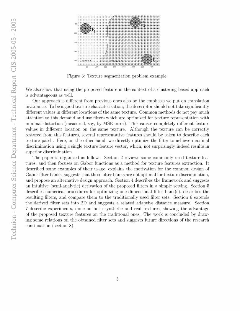
Consider for example figure 3. A illustration of the desirable distances between featurevectors: The neighborhood of point P1 belongs to Texture1, while those of P2 and P3 belongto Texture2. Let d(Pi, Pj) be a distance between associated feature vectors at Pi and Pj .Then ideally,

d(P2, P3) < d(P1, P2) and d(P2, P3) < d(P1, P3).

The validity of this relation depends on the type of metric, the feature vector characterizingthe texture patch etc. Some features and comparison methods are described in section 2.

This work considers the influence of the feature vector (and the associated distancemeasure) on texture discrimination. We restrict ourselves to Gabor features (a commonchoice for texture features, (see section 2.2) and propose a method for designing a Gabor filterset to maximize texture discrimination. The design is made over a simple set of synthetictextures, for which the discrimination is optimized by analytic and numerical methods. Then,we show that the derived filters work well for realistic textures.

Unlike the common modern approach, we characterize a texture by a vector whose compo-nents are the responses of (Gabor) filters and not histograms of local texton cluster identitiesover a region. This way, the decision whether two points belong to the same texture may bemade without additional clustering stage, which results is a faster answer to such queries.

2

Tec

hnio

n -

Com

pute

r Sc

ienc

e D

epar

tmen

t - T

echn

ical

Rep

ort

CIS

-200

5-05

- 2

005

50 100 150 200 250 300 350 400

50

100

150

200

250 Texture 2 Texture 1

Figure 3: Texture segmentation problem example.

We also show that using the proposed feature in the context of a clustering based approachis advantageous as well.

Our approach is different from previous ones also by the emphasis we put on translationinvariance. To be a good texture characterization, the descriptor should not take significantlydifferent values in different locations of the same texture. Common methods do not pay muchattention to this demand and use filters which are optimized for texture representation withminimal distortion (measured, say, by MSE error). This causes completely different featurevalues in different location on the same texture. Although the texture can be correctlyrestored from this features, several representative features should be taken to describe eachtexture patch. Here, on the other hand, we directly optimize the filter to achieve maximaldiscrimination using a single texture feature vector, which, not surprisingly indeed results insuperior discrimination.

The paper is organized as follows: Section 2 reviews some commonly used texture fea-tures, and then focuses on Gabor functions as a method for texture features extraction. Itdescribed some examples of their usage, explains the motivation for the common design ofGabor filter banks, suggests that these filter banks are not optimal for texture discrimination,and propose an alternative design approach. Section 4 describes the framework and suggestsan intuitive (semi-analytic) derivation of the proposed filters in a simple setting. Section 5describes numerical procedures for optimizing one dimensional filter bank(s), describes theresulting filters, and compare them to the traditionally used filter sets. Section 6 extendsthe derived filter sets into 2D and suggests a related adaptive distance measure. Section7 describe experiments, done on both synthetic and real textures, showing the advantageof the proposed texture features on the traditional ones. The work is concluded by draw-ing some relations on the obtained filter sets and suggests future directions of the researchcontinuation (section 8).

3

Tec

hnio

n -

Com

pute

r Sc

ienc

e D

epar

tmen

t - T

echn

ical

Rep

ort

CIS

-200

5-05

- 2

005

2 Background: Texture discrimination methods

Texture discrimination is needed for two main applications: classification and segmentation.The aims of these applications are different but they often use the same texture characteri-zation methods (See 2.1.5 for a short description of feature application methods).

2.1 Texture features

A texture feature associated with some texture patch, is a local descriptor describing sometexture-relevant characteristic of this patch. The patch is thus represented by a vector of suchdescriptors. Many texture features were proposed. A simplistic (but in some context, alsoeffective) method to use the actual grey-levels of pixel’s neighborhood as texture features.Some other approaches, described below, project the image onto another representationspace.

We shall discriminate between patch descriptors, soft neighborhood descriptors and in-direct descriptors

2.1.1 Texture Patch Descriptors

Some of methods are traditionally classified as model based methods , because the pixel’sneighborhood is considered to be a result of some known parametric process. Other methodsdo not use such models and are called non-model based methods .

Some of the popular Model Based Features are

1. Fractal Models [23, 1]. Pentland [23] proved that the fractal dimensions [1] of any objectand its image are equal. From this proof he derived that images may be segmentedinto homogenous parts using a segmentation of their fractal dimension histograms.This approach actually claimed that textured areas may be distinguished by a singleparameter. When opposite examples were provided, additional fractal parameters suchas Lacunarity [1] and directional fractal measurement were proposed.

2. Autoregressive Models [21]. Autoregressive (AR) models consider the pixel’s gray levelvalue as a result of some random process. This way each pixels’ value can be representedas a weighted sum of surrounding pixels. Region classification is done by comparingthe models built for them. Rotation invariant versions were proposed as well. AR is aparticular case of more general MRF approach.

3. Markov Random Fields [3, 29]. A texture is considered to be a realization of a sto-chastic, two dimensional Markov Random field. In a MRF model, the gray level in apixel is a random variable randomized depending on its neighbors. Therefore, sometypical neighborhoods characterizing the texture appear more frequently and may rep-resent the texture. Alternatively, similar to AR models, the parameters specifying thedependency may be used as a representation.

Some of the Non-model-based Features are

4

Tec

hnio

n -

Com

pute

r Sc

ienc

e D

epar

tmen

t - T

echn

ical

Rep

ort

CIS

-200

5-05

- 2

005

1. Grey-level co-occurrence [13]. These methods actually calculate two dimensional his-tograms of the occurrence of the pairs of grey-levels for a given displacement vector(distance and direction). That is, the resulting matrix contains the number of theoccurrences for each possible pair of gray-levels separated by distance d in direction θfor a given texture patch.

2. Frequency domain methods Commonly used features consist of sums of coefficientswithin wedges, rings or sectors of two dimensional power spectra. Additional featuresinclude the characteristics of ”spectral peaks”.

2.1.2 Soft neighborhood descriptors

One often needs to characterize every pixel in the image with respect to the texture itlies on. One straightforward method would be to define a patch around every such pixeland to characterize the pixel using the patch texture features described above. A betterrepresentation would be one which puts more weight on the image properties closer to thepixel (relative to other locations in the patch). Features based on Gabor filters (see section2.2), wavelet and wavelet packet decomposition [2] and other characterizations based onmixed space-frequency descriptors are especially suitable for such tasks. One example ofthe later is Laws’ texture energy filters [15] (which are sets of seven bandpass and high-passdirectional filters, implemented as 5 × 5 masks). A comparative study which consider mostof the common texture features and suggests new sets of filters for specific texture classes isdescribed [27].

2.1.3 Indirect, distribution based, descriptors

It often happens that textures contain several typical sub-patterns, which appear more fre-quently than others. These are commonly named texons. Several texture characterizationmethods rely on the distribution of textons: One popular method is to cluster the (vector)pixel (soft neighborhood) or patch descriptors vectors into several (K) groups (or clusters).This way, every pixel is assigned to some cluster and is given an index. The distributionof such indexes in the neighborhood of the pixel is used as a texture characterization ofthis pixel. This method turned out to be very successful but note that it is not local: thecharacterization depends, in principle, on all image gray levels. The feature vectors thatare clustered may be either Gabor filter responses [19] or even the gray levels in a smallneighborhood themselves [29].

Mean shift clustering is a more modern method of clustering which may be used forindirect texture features generation as well. Here, the number of groups is found in aniterative convergence process. The distribution of the groups in neighborhood of the pixel isused for textures comparison [10].

2.1.4 Comparing texture descriptors

The feature vector descriptions may be compared by several methods. One way would beto use some metric distance d (satisfying symmetry, minimality, triangular inequality andself-similarity). However there are strong evidences that metric distance measurement is

5

Tec

hnio

n -

Com

pute

r Sc

ienc

e D

epar

tmen

t - T

echn

ical

Rep

ort

CIS

-200

5-05

- 2

005

not fully consistent with human perception system. For example, there is no proof that aproperty of triangular inequality exists for human perception [14].

Instead of a metric distance it is possible to compare texture features using some dis-similarity measure, which does not require the Triangle inequality. Practically, many mea-sures are used. Some common methods are Euclidean distance Ln, Mahalanobis distances,correlation, χ2 and Earth Movers distance (EMD) [24]. Some papers suggest building rule-based systems or neural network classifiers [11].

2.1.5 Application of the features

As mentioned earlier, there are two main tasks for texture discrimination systems: recogni-tion and segmentation.

A texture recognition task is divided into two stages: training and recognition. In trainingmany patches of different textures are given together with their classifications. A representa-tion of every texture is constructed. A modern example is the distribution of feature vectors.Then, in the recognition stage, a query patch of some texture is given and its classification isrequired. This may be carried out by finding the distribution of features in the given patchand comparing it to every one of the distributions obtained in training. In this task, muchof the work is done in the feature extraction and in the distribution estimation. Texturerecognition results are usually characterized by a relatively high performance, because a lotof features, for relatively large image areas are considered for a single decision on texturekind [29].

Texture based segmentation usually starts by extracting a large matrix of similaritiesassociated with every pair of pixels (or some rougher image quantization). For an N × Nimage, this matrix is of size N2 ×N2. Then, the segmentation method based on this matrixmay be of different complexities. A simple method could, for example, build a graph whereevery nodes corresponds to a unique pixel. Then, graph edges are added only where thesimilarity between the corresponding feature vectors is high. Then, connected componentsalgorithm partitions the graph (and the corresponding image) into groups. A more complexalgorithm could use less trivial graph partitioning methods such as Normalized Cut [26],edge flow [18], Multi-grid aggregation [25], Active contours and different Byesian criteriabased methods.

2.2 Gabor features

Gabor kernels are commonly used for texture features extraction. Their popularity is moti-vated by the mathematical and the biological properties of Gabor functions.

In 1946, D.Gabor [9] proved that a signal’s specificity simultaneously in time and fre-quency is fundamentally limited by a lower bound on the product of its bandwidth andduration (analogous to indeterminacy relations of quantum mechanics). The bound is

(∆x)(∆ω) ≥ 14π

. He also proved that signals of the form s(t) = e−t2

α2 +iωt achieve the theo-retical limit he found.

Computationally, the Gabor functions form a complete but non-orthogonal basis set andany given function can be expanded in terms of these basic functions.

6

Tec

hnio

n -

Com

pute

r Sc

ienc

e D

epar

tmen

t - T

echn

ical

Rep

ort

CIS

-200

5-05

- 2

005

In 1985 Daugman generalized the Gabor function to the following 2D form to model thereceptive-field profiles of simple cells in the striate cortex[6]:

G(x, y) =1

2πσβe−π

�(x−x0)2

σ2 +(y−y0)2

β2

�−2πi[u0(x−x0)+v0(y−y0)]

(2.1)

These functions, which are spatial bandpass filters with central frequency (u0, v0), achievethe theoretical limit for conjoint resolution of information in the 2D spatial and 2D Fourierdomains.

The specified properties of 2D Gabor functions inspired a search for texture discriminationmethods based on these functions. Porat and Zeevi [22] reviewed several Gabor features andsuggested a texture discrimination method based on two of them. Fogel and Sagi [8] proposeda texture discrimination method, which is based on calculation of the dissimilarity betweenGabor power spectrum of two texture elements. In other words they compute the absolutevalue of the complex Gabor-filtering result and compare the received values. Fogel andSagi were the first to notice that texture features received by this method are locally shiftinvariant. Malik and Perona [20] explained that Gabor features should be non-linear, tomake their recognition properties consistent with human perception. They also mentionedthe Fogel and Sagi method as one of the methods which implement their findings.

2.2.1 Representing texture with oriented Gabor power filters

As it clear from eq. (2.1), Gabor kernel significantly responds to a limited range of signalswhich form a repeating structure in some direction (which is usually denoted as filter’sorientation or direction) and are associated with some frequencies (filters band). The obviousquestion is which filters should be taken to represent all possible textures.

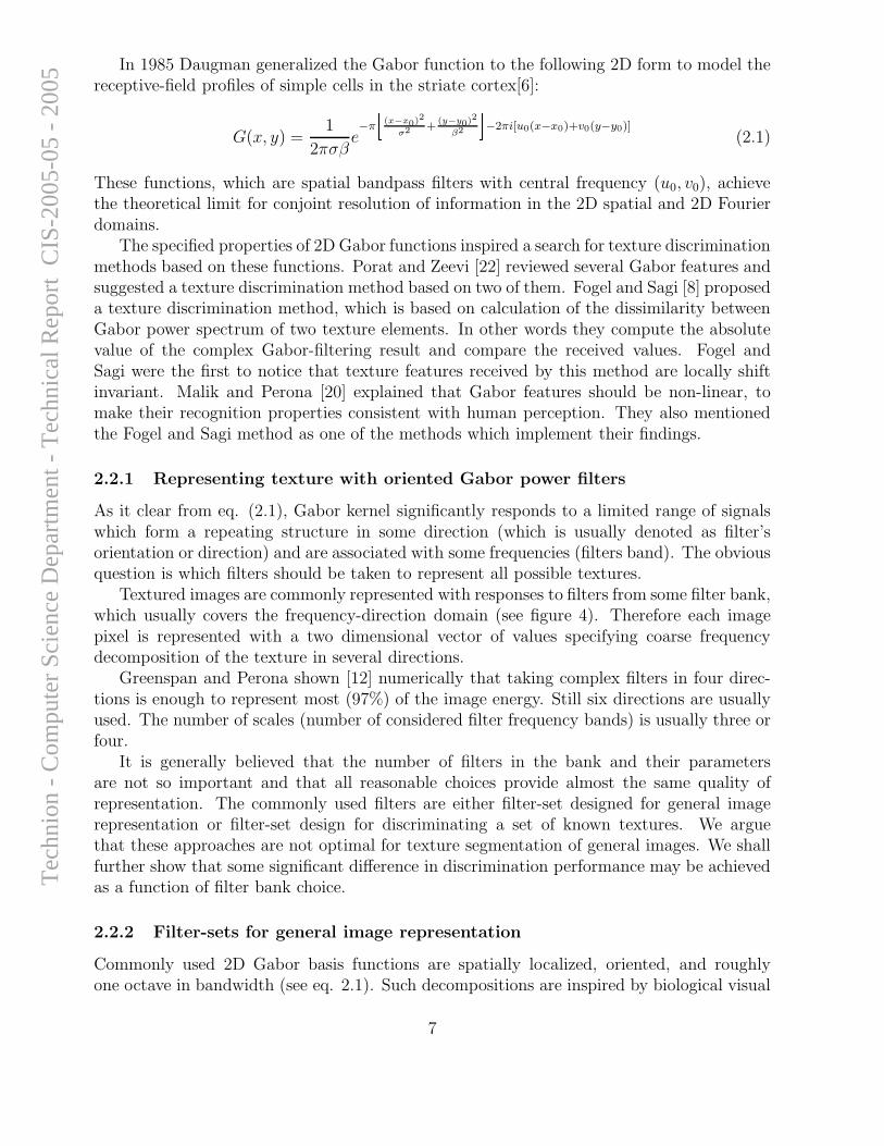
Textured images are commonly represented with responses to filters from some filter bank,which usually covers the frequency-direction domain (see figure 4). Therefore each imagepixel is represented with a two dimensional vector of values specifying coarse frequencydecomposition of the texture in several directions.

Greenspan and Perona shown [12] numerically that taking complex filters in four direc-tions is enough to represent most (97%) of the image energy. Still six directions are usuallyused. The number of scales (number of considered filter frequency bands) is usually three orfour.

It is generally believed that the number of filters in the bank and their parametersare not so important and that all reasonable choices provide almost the same quality ofrepresentation. The commonly used filters are either filter-set designed for general imagerepresentation or filter-set design for discriminating a set of known textures. We arguethat these approaches are not optimal for texture segmentation of general images. We shallfurther show that some significant difference in discrimination performance may be achievedas a function of filter bank choice.

2.2.2 Filter-sets for general image representation

Commonly used 2D Gabor basis functions are spatially localized, oriented, and roughlyone octave in bandwidth (see eq. 2.1). Such decompositions are inspired by biological visual

7

Tec

hnio

n -

Com

pute

r Sc

ienc

e D

epar

tmen

t - T

echn

ical

Rep

ort

CIS

-200

5-05

- 2

005

(a) (b)

Figure 4: (a) The cumulative frequency responses of a bank of Gabor filters, plotted in a2D frequency plane. Each bright spot represents a range of frequencies for which some filterstrongly respond. Note that each ring of spots corresponds to filters with the same radialfrequency. Spot with different distance from the origin but same directions correspondto different scales. This filter bank contains 5 scales and 4 directions. (b) The featurescalculated in every pixel of the given texture. Each greyscale in the right 18 squares equalsto the response magnitude of the filter associated with this square in the pixel with the samecoordinates on the original image (the most left image). The features are calculated usingfilter set of three filters oriented in six different directions. For example the value at position(14, 46) on the third square in the second row is associated with the response to the filterwith the second frequency of the set in the third direction at pixel (14,46) of the originaltexture.

processing [6] and by signal representation considerations. Specifically, Field [7] claimed thatsuch filters are optimal for natural scene images coding: he found that the most compactrepresentation of (a small set of) natural images is achieved when the representation is donewith log-Gabor filters associated with 1.0 octave frequency bands.

Lee [16] showed that 2D Gabor filters with octave steps form a frame. Family of functionsforms a frame when any original signal may be reconstructed in a numerically stable way fromits decomposition coefficients, and the difference between the energy of the reconstructedsignal and the original energy is bounded. A tightness of a frame is specified as a measureof non-variability of the difference between the original and the reconstructed energies. Leefound that a 1.5 octave filters form a tighter frame and that they can be treated as thoughit were an orthonormal base.

2.2.3 Multi-textured images

In this approach [30, 11] all the possible textures are preliminarily known, as well as thebank of all possible Gabor filters. The issue is to select the best filters for the segmentationtask. The general method in this case is to test all the filters on textures’ samples and toselect the most valuable ones into the filter-set.

8

Tec

hnio

n -

Com

pute

r Sc

ienc

e D

epar

tmen

t - T

echn

ical

Rep

ort

CIS

-200

5-05

- 2

005

2.2.4 Some sample implementation of Gabor feature based texture discrimina-tion systems

Many vision systems use texture discrimination by Gabor filters. To illustrate the usage ofthese feature, we now briefly describe three representative examples.

Greenspan et al. [11] The method is based on extraction of texture features for each8 × 8 block of the image and consecutive recognition from database with learningbased algorithms.

In the feature extraction stage the image processed in three scales. In each scale 4absolute values of the responses to different orientations of the same complex log-Gabor filter are obtained. The Fourier transform of theses values, done relating tothe orientation axis, provides rotation invariant representation of the texture on thisscale. The transform also allows to find some ”texture’s direction” which is used todistinguish different orientations of the texture of the same kind. An additional featurefor each scale is the response to Laplacian filter of the same size as the Gabor filter.The result of the feature extracting stage is a 15-dimensional feature vector. The scales(the filters frequencies) are distributed in octave steps, such that the filters bandwidthdoubles for each next high-frequency band.

In the second (recognition) stage the features were clustered along each dimensionusing K-means algorithm and the results were classified using different methods. Theassociation of the patches with texture classes is used for image segmentation andtexture classes recognition.

EMD based image retrieval Rubner [24] uses Gabor features in his database image re-trieval algorithm for searching an image that includes a given texture. In the pre-processing stage of the algorithm, every image passes a feature extraction stage, thefeatures are clustered using K-means algorithm and K resulting features are storedas a representation of the textures which are present in the image. In the retrievalstage some image including only the requested texture is presented to the system, itsfeatures are averaged and the resulting feature vector is EMD-compared (see below) toevery feature vector stored in the database in the preprocessing stage. The images thatone of their feature vectors is close to the query are added to the answer as possiblecandidate.

The EMD (Earth Mover’s Distance) is defined as the minimum amount of work neededto change one feature vector into the other. The ”work” may be defined differentlyfor features of different nature (for example, moving energy between the features ofthe same scale may be defined as cheaper then moving it to other scales). In the caseof Gabor features the resulting distance measure is more justified than the commonlyused metrics that minimize geometrical distance.

Rubner used 24-dimensional feature vectors, constructed from absolute value Gaborresponses to 4 filters frequencies in 6 directions. He also used filters organized in octave-like way and used Fourier-Mellin transform for providing rotation and scale invarianceto the resulting feature vectors.

9

Tec

hnio

n -

Com

pute

r Sc

ienc

e D

epar

tmen

t - T

echn

ical

Rep

ort

CIS

-200

5-05

- 2

005

Normalized cut method [26, 19] In [26] the authors acted in a more or less common way- they calculated Gabor-like features of the input image and passed these features to thesegmentation mechanism. They used 18 DOG absolute value features, received using 3filters in 6 directions. DOG - Difference of non-isotropic Gaussians are complex filterswhich are similar to the Gabor filters with one cycle of the sine inside the meaningfularea of the filter.

In the segmentation stage a connected full graph is built, while each graph node repre-senting a pixel of the image and every edge represents a ”likelihood” for the two pixelsto be a part of the same object. The edge value is set as an exponential function of(minus) the scalar product between the pixels’ feature vectors. This way, pixels withsimilar feature vectors are getting a high edge value. The goal of graph segmentationmethods is to find a minimal cut which is a combination of edges having minimal sumof edge values (i.e. find the least alike pairs of pixels), and removing these edges di-vides the graph into two unconnected subgraphs. The advantage of the normalized cutmethod is that it considers two aspects of graph segmentation: minimal cut (i.e. betterseparation) and preferring segments of large size. The normalized cut process dividesthe weighted graph into two subgraphs, such that the cut between the subgraphs,normalized by the total ”connectivity”, is minimal.

In a second paper [19] the texture features are analyzed using the distribution basedtexture descriptors (see 2.1.3). The Gabor feature vectors are not directly comparedas in the first article, but divided into K clusters and each image pixel is assigned toone of these clusters. Using the Delaunay triangulation a local scale is found for everypixel, and the histogram of clusters distribution in the neighborhood of this local scalesize is attached to each pixel as a descriptor. A ”likelihood” for the pixels to be a partof the same object (denoted as texture cue) is calculated by χ2 test on the descriptorhistograms of the pixels. In this method in addition to the texture cues, additional,edge detection based, contour cues are also considered. The segmentation is done using”normalized cut” method, while the edge value is set to be the exponent of the productof contour and texture cues for the pixel pair.

10

Tec

hnio

n -

Com

pute

r Sc

ienc

e D

epar

tmen

t - T

echn

ical

Rep

ort

CIS

-200

5-05

- 2

005

3 Our approach

This work is done in the context of the following common framework for texture discrimi-nation: the texture image is filtered by several (complex) Gabor filters and a feature vectoris constructed with the absolute values of the responses as components. The discriminationbetween textures uses only these feature vectors and relies on simple procedures to decidewhether two vectors are associated with the same texture. Specifically, such a proceduredecides that the texture in two points is of the same type, if the Euclidean (or Mahalanobis)distances between the corresponding feature vectors is lower than some threshold.

This work focuses on the design of the Gabor filters set. As mentioned above, the commonchoices are made for optimizing the filter design with respect to image representation (inMSE sense). We argue that the best filters for texture discrimination are different than thoseused for representation and shall indeed propose a set of Gabor filter, which is different thatthe commonly used sets.

The response of a filter to some texture may take a range of values. We shall say thata filter (or a filter set) discriminate between two textures if the ranges of values associatedwith these two textures, are disjoint. We shall look for filters maximizing the discriminationbetween different textures, in a well defined sense described below; see section 4.2. To thatend, we develop an analytical expression for the range of response values of a 1D Gaborfilter to simple signals (e.g. Sine waves). We use these ranges to specify the best filter sets,which separate best between the simple signals. The filter sets are derived by numerical andsemi-analytical methods, which lead to similar results. The resulting filter sets are differentthan the traditional ones.

In a sense, the design of filter sets for specific textures [30] is related to our work. Onemain difference is that we model the signal and estimate the variation analytically. Anotherdifference is that unlike the iterative, heuristic design, suggested in [30], we use a globalprocess for the optimization.

Our work can be considered to be an investigation into the translation sensitivity ofGabor filters. While the absolute value of Gabor filtered signal will never be truly shiftinvariant, its variability may be bounded in relatively small ranges, such that for a relativelyfar values we would be able to say that they belong to different textures.

Essentially, traditional texture discrimination methods consider the filter response inqualitative form. For example, if the texture is simple (e.g. sinusoidal), they are interestedin the filter that react maximally to it, and not much in the actual response size. In con-trast to these methods but not unlike the modern, distribution based approaches, we modelthe actual response and therefore can make a finer, “super resolution” like, discriminationbetween textures. Analogously to super-resolution methods using several measurements cor-responding to the same brightness, the resulting filters turn out to be highly overlapping infrequency coverage. This leads, as we shall see, to better discrimination.

As described above, modern texture characterization methods rely on distributions offilter response. Such methods were proved to be insensitive to the type of texture features[29], provided that a sufficient number of textons is allowed. We, on the other hand, areinterested in finding the best feature and therefore shall evaluate the proposed ones usingdirect methods (and not using distributions). It is likely that less complex distributions(with a lower number of textons) could be built with better features.

11

Tec

hnio

n -

Com

pute

r Sc

ienc

e D

epar

tmen

t - T

echn

ical

Rep

ort

CIS

-200

5-05

- 2

005

4 A filter response to harmonic input analysis

We start by considering the range of responses associated with one 1D filter and one sim-ple signal. The simple signals considered as a model of texture are either Sines signals orcombination of them. The discrimination study is done in the context of specific sets of sig-nals associated with [fmin, fmax] frequency range and [Amin, Amax] amplitudes range. Theseranges are latter referred to as the framework. Our goal is to maximize the number of signalpairs which may be distinguished. The desired result is a set of filter’s parameters, dependingon the prespecified number of filters and the parameters fmin, fmax, Amin, Amax.

We first focus on a few simple cases, allowing intuition to the Gabor filters signal dis-crimination capabilities and providing computational advantages in the final optimization.For a simple case of a single harmonic signal with known amplitude we can find the optimalsingle filter analytically. Using the acquired intuition we developed a semi-analytical methodfor building a filter set for discriminating between single harmonic signals with unspecifiedamplitudes. The resulting filter set is very similar to the one obtained from the full numericalsearch on the filter parameters domain.

We also provide an expression for Gabor filter response bounds to dual-harmonic signalsand multi-harmonic signals. Estimates based on these expressions allows us to understandthe responses behavior and imply that the filters, obtained for single harmonic signals, per-form well for the multi harmonic case too. As we shall see later, these filters perform wellfor distinguishing between real textures as well.

4.1 A single filter response to Sine signal

Consider a complex Gabor filter hk,σ2(x) = 1√2πσ2

e−x2

2σ2 +ikx , and a signal gA,m(x) = Asin(mx).

The (complex) filter response is highly variable depending on location but its absolute value

rA,m,k,σ2(x) = |hk,σ2(x) ∗ gA,m(x)| (4.1)

= Ae−(k2+m2)σ2

2

√

ch2(kmσ2) − cos2(mx)

is more stable (see Appendix A for derivation). Here we consider only the absolute value ofthe response and refer to it simply as the response.

This response varies with location (x coordinate) and depends on the relative phase ofthe Sine input signal with respect to the filter location (x = 0). This change is undesirable,but still unavoidable. It can be shown that the range of responses is bounded by

A

2

{

e−(k−m)2σ2

2 + e−(k+m)2σ2

2

}

> rA,m,k,σ2(x) >A

2

{

e−(k−m)2σ2

2 − e−(k+m)2σ2

2

}

. (4.2)

These bounds are tight. The response varies around a middle value,

rA,m,k,σ2 =A

2e

−(k−m)2σ2

2 , (4.3)

with a maximal deviation

∆rA,m,k,σ2 = Ae−(k+m)2σ2

2 . (4.4)

12

Tec

hnio

n -

Com

pute

r Sc

ienc

e D

epar

tmen

t - T

echn

ical

Rep

ort

CIS

-200

5-05

- 2

005

−2.5 −2 −1.5 −1 −0.5 0 0.5 1 1.50

0.05

0.1

0.15

0.2

0.25

0.3

0.35

0.4

0.45

0.5

r 1,ω

,k,σ

2

log(k)log(ω1) log(ω

2) log(ω

3) log(ω

4)log(ω

5)

r1

r1’ r

2

r2’

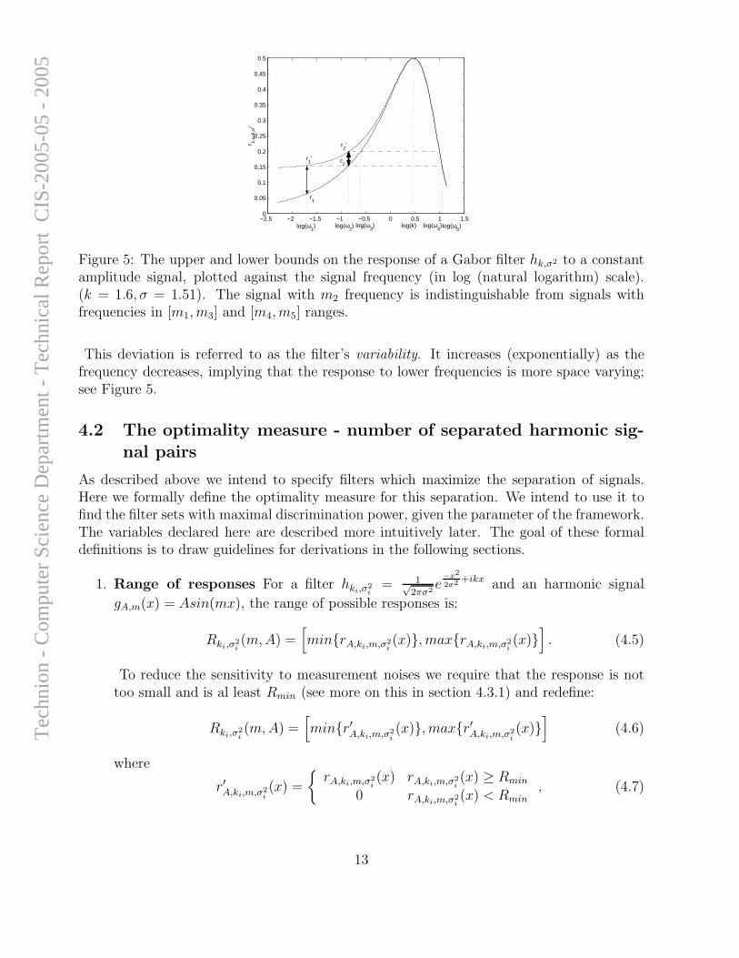
Figure 5: The upper and lower bounds on the response of a Gabor filter hk,σ2 to a constantamplitude signal, plotted against the signal frequency (in log (natural logarithm) scale).(k = 1.6, σ = 1.51). The signal with m2 frequency is indistinguishable from signals withfrequencies in [m1, m3] and [m4, m5] ranges.

This deviation is referred to as the filter’s variability. It increases (exponentially) as thefrequency decreases, implying that the response to lower frequencies is more space varying;see Figure 5.

4.2 The optimality measure - number of separated harmonic sig-

nal pairs

As described above we intend to specify filters which maximize the separation of signals.Here we formally define the optimality measure for this separation. We intend to use it tofind the filter sets with maximal discrimination power, given the parameter of the framework.The variables declared here are described more intuitively later. The goal of these formaldefinitions is to draw guidelines for derivations in the following sections.

1. Range of responses For a filter hki,σ2i

= 1√2πσ2

e−x2

2σ2 +ikx and an harmonic signal

gA,m(x) = Asin(mx), the range of possible responses is:

Rki,σ2i(m, A) =

[

min{rA,ki,m,σ2i(x)}, max{rA,ki,m,σ2

i(x)}

]

. (4.5)

To reduce the sensitivity to measurement noises we require that the response is nottoo small and is al least Rmin (see more on this in section 4.3.1) and redefine:

Rki,σ2i(m, A) =

[

min{r′A,ki,m,σ2i(x)}, max{r′A,ki,m,σ2

i(x)}

]

(4.6)

where

r′A,ki,m,σ2i(x) =

{

rA,ki,m,σ2i(x) rA,ki,m,σ2

i(x) ≥ Rmin

0 rA,ki,m,σ2i(x) < Rmin

, (4.7)

13

Tec

hnio

n -

Com

pute

r Sc

ienc

e D

epar

tmen

t - T

echn

ical

Rep

ort

CIS

-200

5-05

- 2

005

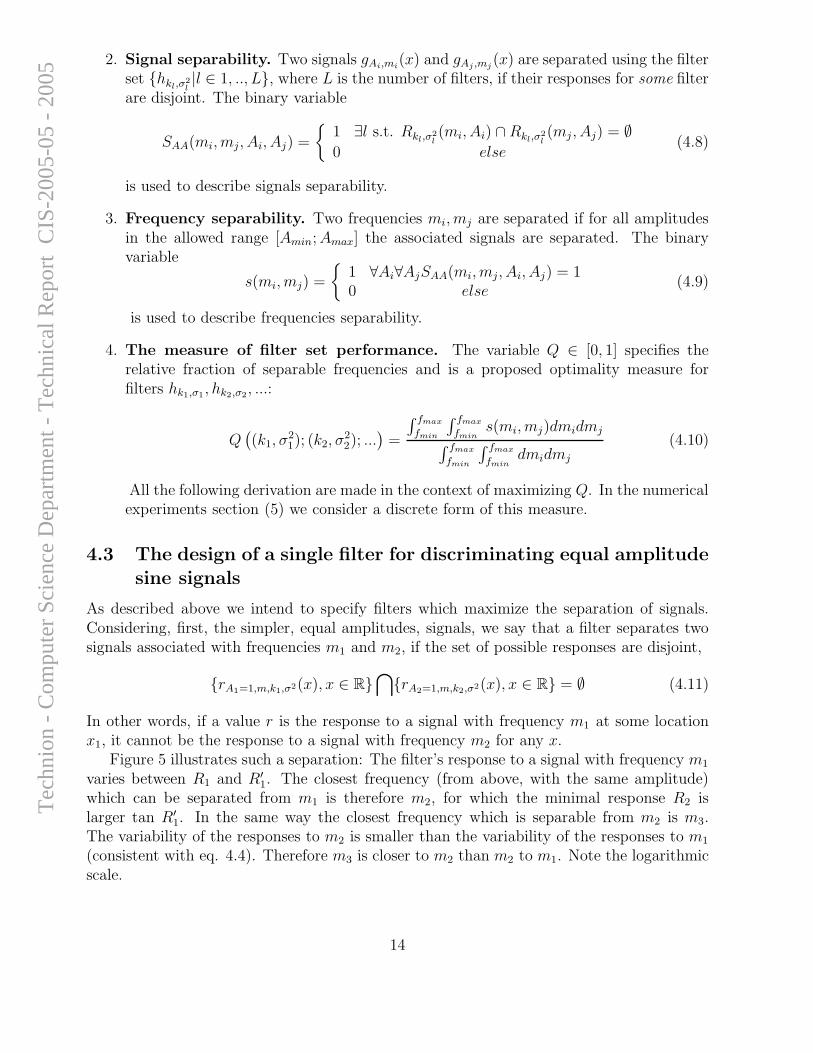
2. Signal separability. Two signals gAi,mi(x) and gAj ,mj

(x) are separated using the filterset {hkl,σ

2l|l ∈ 1, .., L}, where L is the number of filters, if their responses for some filter

are disjoint. The binary variable

SAA(mi, mj, Ai, Aj) =

{

1 ∃l s.t. Rkl,σ2l(mi, Ai) ∩ Rkl,σ

2l(mj , Aj) = ∅

0 else(4.8)

is used to describe signals separability.

3. Frequency separability. Two frequencies mi, mj are separated if for all amplitudesin the allowed range [Amin; Amax] the associated signals are separated. The binaryvariable

s(mi, mj) =

{

1 ∀Ai∀AjSAA(mi, mj, Ai, Aj) = 10 else

(4.9)

is used to describe frequencies separability.

4. The measure of filter set performance. The variable Q ∈ [0, 1] specifies therelative fraction of separable frequencies and is a proposed optimality measure forfilters hk1,σ1, hk2,σ2, ...:

Q(

(k1, σ21); (k2, σ

22); ...

)

=

∫ fmax

fmin

∫ fmax

fmins(mi, mj)dmidmj

∫ fmax

fmin

∫ fmax

fmindmidmj

(4.10)

All the following derivation are made in the context of maximizing Q. In the numericalexperiments section (5) we consider a discrete form of this measure.

4.3 The design of a single filter for discriminating equal amplitudesine signals

As described above we intend to specify filters which maximize the separation of signals.Considering, first, the simpler, equal amplitudes, signals, we say that a filter separates twosignals associated with frequencies m1 and m2, if the set of possible responses are disjoint,

{rA1=1,m,k1,σ2(x), x ∈ R}⋂

{rA2=1,m,k2,σ2(x), x ∈ R} = ∅ (4.11)

In other words, if a value r is the response to a signal with frequency m1 at some locationx1, it cannot be the response to a signal with frequency m2 for any x.

Figure 5 illustrates such a separation: The filter’s response to a signal with frequency m1

varies between R1 and R′1. The closest frequency (from above, with the same amplitude)

which can be separated from m1 is therefore m2, for which the minimal response R2 islarger tan R′

1. In the same way the closest frequency which is separable from m2 is m3.The variability of the responses to m2 is smaller than the variability of the responses to m1

(consistent with eq. 4.4). Therefore m3 is closer to m2 than m2 to m1. Note the logarithmicscale.

14

Tec

hnio

n -

Com

pute

r Sc

ienc

e D

epar

tmen

t - T

echn

ical

Rep

ort

CIS

-200

5-05

- 2

005

−3 −2.5 −2 −1.5 −1 −0.5 0 0.5 1 1.50

0.1

0.2

0.3

0.4

0.5

0.6

0.7

0.8

0.9

1

−3 −2.5 −2 −1.5 −1 −0.5 0 0.5 1 1.50

0.05

0.1

0.15

0.2

0.25

0.3

0.35

0.4

0.45

0.5

(a) (b)

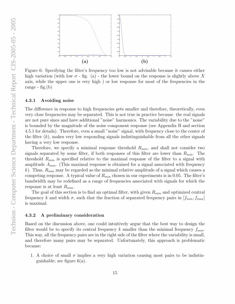
Figure 6: Specifying the filter’s frequency too low is not advisable because it causes eitherhigh variation (with low σ - fig. (a) - the lower bound on the response is slightly above Xaxis, while the upper one is very high ) or low response for most of the frequencies in therange - fig.(b)

4.3.1 Avoiding noise

The difference in response to high frequencies gets smaller and therefore, theoretically, evenvery close frequencies may be separated. This is not true in practice because the real signalsare not pure sines and have additional ”noise” harmonics. The variability due to the ”noise”is bounded by the magnitude of the noise component response (see Appendix B and section4.5.1 for details). Therefore, even a small ”noise” signal, with frequency close to the center ofthe filter (k), makes very low responding signals indistinguishable from all the other signalshaving a very low response.

Therefore, we specify a minimal response threshold Rmin, and shall not consider twosignals separated by some filter, if both responses of this filter are lower than Rmin. Thethreshold Rmin is specified relative to the maximal response of the filter to a signal withamplitude Amin. (This maximal response is obtained for a signal associated with frequencyk). Thus, Rmin may be regarded as the minimal relative amplitude of a signal which causes acompeting response. A typical value of Rmin chosen in our experiments is in 0.05. The filter’sbandwidth may be redefined as a range of frequencies associated with signals for which theresponse is at least Rmin.

The goal of this section is to find an optimal filter, with given Rmin and optimized centralfrequency k and width σ, such that the fraction of separated frequency pairs in [fmin, fmax]is maximal.

4.3.2 A preliminary consideration

Based on the discussion above, one could intuitively argue that the best way to design thefilter would be to specify its central frequency k smaller than the minimal frequency fmin.This way, all the frequency pairs are in the right side of the filter where the variability is small,and therefore many pairs may be separated. Unfortunately, this approach is problematicbecause:

1. A choice of small σ implies a very high variation causing most pairs to be indistin-guishable; see figure 6(a).

15

Tec

hnio

n -

Com

pute

r Sc

ienc

e D

epar

tmen

t - T

echn

ical

Rep

ort

CIS

-200

5-05

- 2

005

m m’ m’’

∆ m

∆ rA,m’,k,σ2

∆ rA,m,k,σ2

∆ rA,m’’,k,σ2

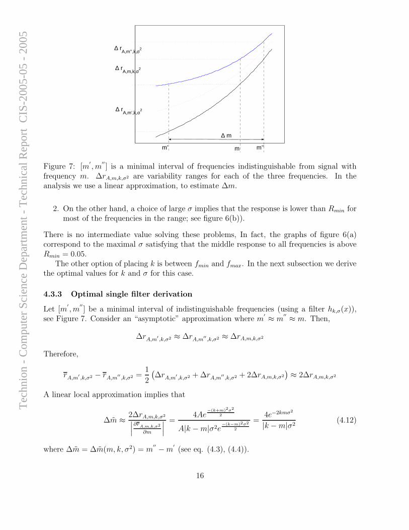
Figure 7: [m′

, m′′

] is a minimal interval of frequencies indistinguishable from signal withfrequency m. ∆rA,m,k,σ2 are variability ranges for each of the three frequencies. In theanalysis we use a linear approximation, to estimate ∆m.

2. On the other hand, a choice of large σ implies that the response is lower than Rmin formost of the frequencies in the range; see figure 6(b)).

There is no intermediate value solving these problems, In fact, the graphs of figure 6(a)correspond to the maximal σ satisfying that the middle response to all frequencies is aboveRmin = 0.05.

The other option of placing k is between fmin and fmax. In the next subsection we derivethe optimal values for k and σ for this case.

4.3.3 Optimal single filter derivation

Let [m′

, m′′

] be a minimal interval of indistinguishable frequencies (using a filter hk,σ(x)),see Figure 7. Consider an “asymptotic” approximation where m

′ ≈ m′′ ≈ m. Then,

∆rA,m′,k,σ2 ≈ ∆rA,m

′′,k,σ2 ≈ ∆rA,m,k,σ2

Therefore,

rA,m′,k,σ2 − rA,m

′′,k,σ2 =

1

2

(

∆rA,m′,k,σ2 + ∆rA,m

′′,k,σ2 + 2∆rA,m,k,σ2

)

≈ 2∆rA,m,k,σ2

A linear local approximation implies that

∆m ≈ 2∆rA,m,k,σ2∣

∣

∣

∂rA,m,k,σ2

∂m

∣

∣

∣

=4Ae

−(k+m)2σ2

2

A|k − m|σ2e−(k−m)2σ2

2

=4e−2kmσ2

|k − m|σ2(4.12)

where ∆m = ∆m(m, k, σ2) = m′′ − m

′

(see eq. (4.3), (4.4)).

16

Tec

hnio

n -

Com

pute

r Sc

ienc

e D

epar

tmen

t - T

echn

ical

Rep

ort

CIS

-200

5-05

- 2

005

A higher discriminability is obtained if ∆m is smaller. Therefore its value is sometimes

referred to as the filter indiscriminability. Note that near the filter’s frequency k,∂rA,m,k,σ2

∂m≈

0 and the range of non separability is wider. This problem is latter resolved using additionalfilters. Note that if a frequency is non separable from any other frequency, then its ∆m isstill fmax − fmin and not infinity. Therefore, the indistinguishability is redefined

∆m = min{∆m, fmax − fmin} (4.13)

As mentioned earlier, our goal is to segregate the maximum possible amount of frequencypairs m1, m2 ∈ [fmin, fmax]. As it is clear from figure 5 that there are two ranges of signalfrequencies which respond similarly to signal m2 - the first is m ∈ [m1, m3] and the secondis m ∈ [m4, m5]. For simplicity we ignore the second range of signals and consider everysignal in [fmin, fmax] to be distinguishable from the signal with frequency m if it’s fartherthan ∆m(m, k, σ)/2 from m. I.e. in case on figure 5 we consider m2 separable from everyfrequency smaller than m1 or larger than m3. With this simplification, the fraction ofindistinguishable signal pairs is (proportional to)

∫ fmax

fmin

∆m(m, k, σ2)dm, (4.14)

and the filter which minimizes this measure, maximizes 4.10 and is thus optimal one.By symmetry, adding the ignored second range of indistinguishable signals, change (4.14)

expression by a multiplicative constant, and hence does not matter for the optimal choice.Requiring that the response is above the threshold Rmin, is approximately equivalent to

rA,m,k,σ2 > Rmin, ∀m ∈ [fmin, fmax], (4.15)

which, considering the filter’s unimodal response, is satisfied if

rA,k,fmin= rA,k,fmax = Rmin. (4.16)

Choosing these minimal responses in the range endpoints specifies the filter’s parameters as:

k =fmin + fmax

2; σ2 = − 8log(Rmin)

(fmax − fmin)2. (4.17)

This choice provides filter parameters which are close to the optimal ones, minimizing(4.14) expression. As explained below (section 5), the values fmax = π, fmin = .1 andRmin = .05 are good choice for practical texture discrimination tasks. These choices lead toa filter associated with k = 1.62 and σ2 = 2.59, which are indeed close to the, numericallyobtained, optimal single filter parameters, which are k = 1.61 and σ2 = 2.31. See Figure 5for a plot of this filter response.

This filter turns out to be optimal due to the following considerations: Increasing σbeyond the value (4.17) contradicts the constraint (4.16). Decreasing it increases ∆m. In-creasing k require to decrease σ to satisfy (4.16) again. In Appendix D it is shown thatincreasing k and decreasing σ (and preserving rA,k,fmin

= Rmin) causes a bigger ∆m forevery m, and therefore the filter can separate less frequency pairs (see 4.14).

17

Tec

hnio

n -

Com

pute

r Sc

ienc

e D

epar

tmen

t - T

echn

ical

Rep

ort

CIS

-200

5-05

- 2

005

Discriminability of sin(m1x) from sin(m

2x) using a single filter

m1

m2

.05 .1 .15 .2 .25 .3

.05

.1

.15

.2

.25

.3

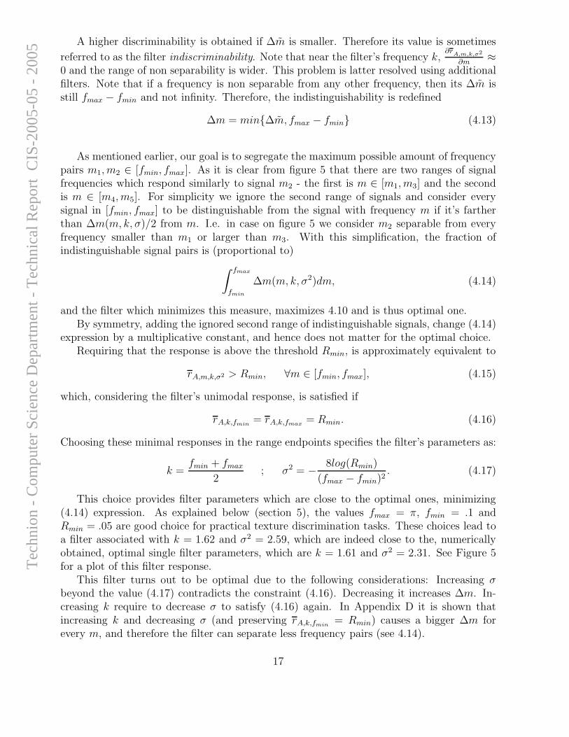
Figure 8: The discriminability of a single filter. For signal pairs, where the frequency of thefirst signal is along x axis and the frequency of the second signal is along y axis, white pixelvalue means that the signals are distinguishable using single filter and black pixel value meansthey are not. Most of the indistinguishable signal pairs are associated with similar signalfrequencies or with signal frequencies which are symmetric around the filter’s frequency (asranges [m1, m3] and [m4, m5] on figure 5)

The conclusion is that any change of the filter specified by (4.17) degrades its discrim-inability. Thus a single filter for best discrimination of single sine signals with equal am-plitudes in an interval [fmin, fmax] for a preset Rmin response is specified by (4.17). Theseparating power of a single filter is illustrated in Figure 8 where pairs of indistinguishablefrequencies are colored dark. As we shall see latter a combination of filters may improvediscriminability.

4.4 The design of a filter-set for signals with a single harmonic

and arbitrary amplitudes

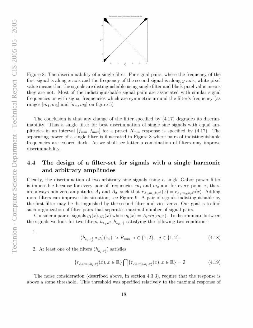
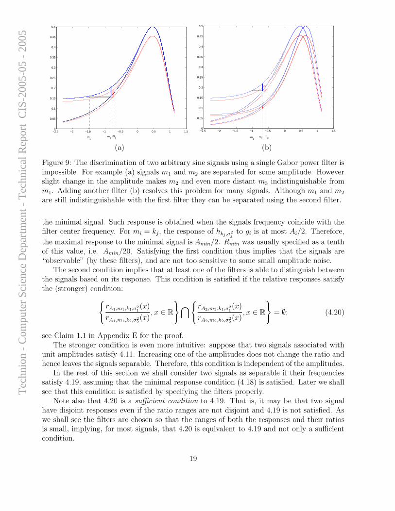
Clearly, the discrimination of two arbitrary sine signals using a single Gabor power filteris impossible because for every pair of frequencies m1 and m2 and for every point x, thereare always non-zero amplitudes A1 and A2, such that rA1,m1,k,σ2(x) = rA2,m2,k,σ2(x). Addingmore filters can improve this situation, see Figure 9. A pair of signals indistinguishable bythe first filter may be distinguished by the second filter and vice versa. Our goal is to findsuch organization of filter pairs that separates maximal number of signal pairs.

Consider a pair of signals g1(x), g2(x) where gi(x) = Aisin(mix). To discriminate betweenthe signals we look for two filters, hk1,σ2

1, hk2,σ2

2satisfying the following two conditions:

1.|(hkj ,σ2

j∗ gi)(x0)| > Rmin i ∈ {1, 2}, j ∈ {1, 2}. (4.18)

2. At least one of the filters (hkj ,σ2j) satisfies

{rA1,m1,kj ,σ2j(x), x ∈ R}

⋂

{rA2,m2,kj ,σ2j(x), x ∈ R} = ∅ (4.19)

The noise consideration (described above, in section 4.3.3), require that the response isabove a some threshold. This threshold was specified relatively to the maximal response of

18

Tec

hnio

n -

Com

pute

r Sc

ienc

e D

epar

tmen

t - T

echn

ical

Rep

ort

CIS

-200

5-05

- 2

005

−2.5 −2 −1.5 −1 −0.5 0 0.5 1 1.50

0.05

0.1

0.15

0.2

0.25

0.3

0.35

0.4

0.45

0.5

m1 m

2 m

3

−2.5 −2 −1.5 −1 −0.5 0 0.5 1 1.50

0.05

0.1

0.15

0.2

0.25

0.3

0.35

0.4

0.45

0.5

m1 m

2m

3

(a) (b)

Figure 9: The discrimination of two arbitrary sine signals using a single Gabor power filter isimpossible. For example (a) signals m1 and m2 are separated for some amplitude. Howeverslight change in the amplitude makes m2 and even more distant m3 indistinguishable fromm1. Adding another filter (b) resolves this problem for many signals. Although m1 and m2

are still indistinguishable with the first filter they can be separated using the second filter.

the minimal signal. Such response is obtained when the signals frequency coincide with thefilter center frequency. For mi = kj, the response of hkj ,σ2

jto gi is at most Ai/2. Therefore,

the maximal response to the minimal signal is Amin/2. Rmin was usually specified as a tenthof this value, i.e. Amin/20. Satisfying the first condition thus implies that the signals are“observable” (by these filters), and are not too sensitive to some small amplitude noise.

The second condition implies that at least one of the filters is able to distinguish betweenthe signals based on its response. This condition is satisfied if the relative responses satisfythe (stronger) condition:

{

rA1,m1,k1,σ21(x)

rA1,m1,k2,σ22(x)

, x ∈ R

}

⋂

{

rA2,m2,k1,σ21(x)

rA2,m2,k2,σ22(x)

, x ∈ R

}

= ∅; (4.20)

see Claim 1.1 in Appendix E for the proof.The stronger condition is even more intuitive: suppose that two signals associated with

unit amplitudes satisfy 4.11. Increasing one of the amplitudes does not change the ratio andhence leaves the signals separable. Therefore, this condition is independent of the amplitudes.

In the rest of this section we shall consider two signals as separable if their frequenciessatisfy 4.19, assuming that the minimal response condition (4.18) is satisfied. Later we shallsee that this condition is satisfied by specifying the filters properly.

Note also that 4.20 is a sufficient condition to 4.19. That is, it may be that two signalhave disjoint responses even if the ratio ranges are not disjoint and 4.19 is not satisfied. Aswe shall see the filters are chosen so that the ranges of both the responses and their ratiosis small, implying, for most signals, that 4.20 is equivalent to 4.19 and not only a sufficientcondition.

19

Tec

hnio

n -

Com

pute

r Sc

ienc

e D

epar

tmen

t - T

echn

ical

Rep

ort

CIS

-200

5-05

- 2

005

The following calculations bring this condition into a simpler form, similar to that of thediscriminability measure (4.12) and allow relatively simple optimization on {~k, ~σ2}1 para-meters. Note, that since the rA,m,k,σ2(x) = Ar1,m,k,σ2(x), the ratio expression is amplitudeindependent, although its derivation is based on signals with various amplitudes.

4.4.1 An expression for indistinguishability

The ratio of two Gabor filters responses to a signal gA,m(x) = Asin(mx), is bounded for anyx by the following upper (G+) and lower (G−) expressions, derived using (4.3)(4.4):

G+(m,~k, ~σ2) = e−(k2

1+m2)σ21−(k2

2+m2)σ22

2ch(mk1σ

21)

sh(mk2σ22)

G−(m,~k, ~σ2) = e−(k2

1+m2)σ21−(k2

2+m2)σ22

2sh(mk1σ

21)

ch(mk2σ22)

As done before (see 4.3) and (4.4), it is convenient to describe this (relative) response range

using its middle response G(m,~k, ~σ2) and its variation ∆G(m,~k, ~σ2):

G(m,~k, ~σ2) =G+(m,~k, ~σ2) + G−(m,~k, ~σ2)

2

∆G(m,~k, ~σ2) =G+(m,~k, ~σ2) − G−(m,~k, ~σ2)

2

The sensitivity of the middle response to frequency may be quantified by its derivative(in analogy to the derivation of (4.12))

∂G(m,~k, ~σ2)

∂m= e−

(k21+m2)σ2

1−(k22+m2)σ2

22

m(σ22 − σ2

1)sh(2mα2) − 2α2ch(2mα2)

sh2(2mα2)ch [m(α1 + α2)]

+e−

(k21+m2)σ2

1−(k22+m2)σ2

22

sh(2mα2)(α1 + α2)sh [m(α1 + α2)] ,

where αi = kiσ2i . The indiscriminability measure quantifying the undistinguishable difference

in frequency is:

∆m =∆G(m,~k, ~σ2)∣

∣

∣

∂G(m,~k, ~σ2)∂m

∣

∣

∣

(4.21)

=ch [m(α1 − α2)]

[m(σ22 − σ2

1) − 2α2coth(2mα2)] ch [m(α1 + α2)] + (α1 + α2)sh [m(α1 + α2)].

As before (see explanation for (4.13)) ∆m = min{∆m, fmax − fmin}1We denote ~k = (k1, k2) and ~σ2 = (σ2

1, σ2

2)

20

Tec

hnio

n -

Com

pute

r Sc

ienc

e D

epar

tmen

t - T

echn

ical

Rep

ort

CIS

-200

5-05

- 2

005

4.4.2 Some useful approximations

We would like to to minimize cumulative indistinguishability (4.14) -∫

∆m(m,~k, ~σ2)dm overall filter parameters k1, k2, σ

21, σ

22. While we can look for this minimum, numerically, by a

dense search over the 4 dimensional parameters space, we prefer to find also some shortcuts,which will be especially useful for the design of larger filter banks.

Reducing the search to two parameters - We first observed that specifying ki (i =1, 2), the cumulative indistinguishability is minimized by choosing the parameters σ2

i

(i = 1, 2) as the highest satisfying (4.15). This observation is consistent with theresult obtained for single amplitude Sine signal analysis and with intuition: Filterswith bigger σ2 have smaller variability. Unfortunately, we were not able to formallyprove this claim, but it is verified by our numerical tests.

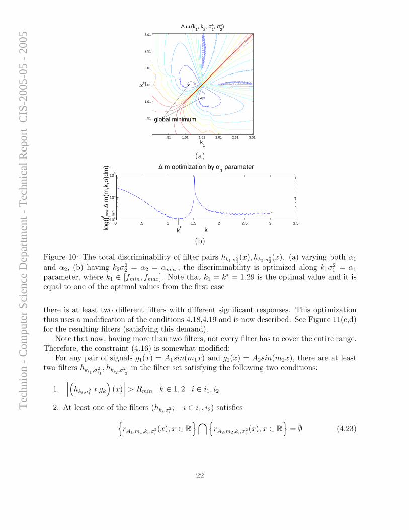
Using this observation we may plot the cumulative indistinguishability∫

∆m(m,~k, ~σ2)dmas a function of only two parameters k1 and k2. See Figure 10(a). For the chosen fre-quency range m ∈ [.2, 3/14] the optimal parameters are k1 = 1.61 and k2 = 1.29 (orvise versa due to symmetry).

Reducing the search to one parameter - Note that k1 gets the same value obtainedfor a single optimal filter (see (4.17)). This is somewhat expected due to the followingargument. For large α (say, larger than 5, which is common for most considered filters),ch [m(α2 + α1)] ≈ sh [m(α2 + α1)] and coth(2mα2) ≈ 1 leading to the approximation

∆m ≈ 1

|m(σ22 − σ2

1) + (α1 − α2)|· ch [m(α1 − α2)]

ch [m(α1 + α2)](4.22)

∆m = min{∆m, fmax − fmin}

The term ch [m(α1 + α2)] have a dominant influence on the size of ∆m. To minimize∆m, it should be larger which happens when its argument, m(α1 + α2) is maximal.Both α1 and α2 are bounded with (4.17) because of (4.15). They cannot get the samevalue because then, they will have equal k and σ2, making ∆m large due to the firstpart of the expression. Therefore only one of α1, α2 can get maximal value. Lettingα2 = αmax and setting k2, σ

22 according to (4.17), we are left with one parameter, α1.

Performing a one parameter optimization over α1 which can only take values smallerthan α2 while hk1,σ2

1satisfies (4.15), we varied k1, and updated σ2

1 accordingly, lookingfor minimal value of integral (4.14).

The results obtained using this faster, approximation based method (see figure 10(b)) arethe same as obtained from the search on k1, k2 (figure 10(a))and also similar to the resultsof full search on k1, k2, σ

21, σ

22 , maximizing explicitly the number of separated signal pairs,

described in the next section.

4.4.3 Three filters and more

For more than two filters the analysis seems too complex and we rely on numerical opti-mization. Essentially, the optimization looks for a set of filters such that for every frequency

21

Tec

hnio

n -

Com

pute

r Sc

ienc

e D

epar

tmen

t - T

echn

ical

Rep

ort

CIS

-200

5-05

- 2

005

.51 1.01 1.61 2.01 2.51 3.01

.51

1.01

1.61

2.01

2.51

3.01

∆ ω (k1, k

2, σ

12, σ

22)

k1

k 2

global minimum

(a)

0 .5 1 1.5 2 2.5 3 3.510

1

102

103

∆ m optimization by α1 parameter

klog(

∫f max

f min

∆ m

(m,k

,σ)d

m)

k*

(b)

Figure 10: The total discriminability of filter pairs hk1,σ21(x), hk2,σ2

2(x). (a) varying both α1

and α2, (b) having k2σ22 = α2 = αmax, the discriminability is optimized along k1σ

21 = α1

parameter, where k1 ∈ [fmin, fmax]. Note that k1 = k∗ = 1.29 is the optimal value and it isequal to one of the optimal values from the first case

there is at least two different filters with different significant responses. This optimizationthus uses a modification of the conditions 4.18,4.19 and is now described. See Figure 11(c,d)for the resulting filters (satisfying this demand).

Note that now, having more than two filters, not every filter has to cover the entire range.Therefore, the constraint (4.16) is somewhat modified:

For any pair of signals g1(x) = A1sin(m1x) and g2(x) = A2sin(m2x), there are at leasttwo filters hki1

,σ2i1, hki2

,σ2i2

in the filter set satisfying the following two conditions:

1.∣

∣

∣

(

hki,σ2i∗ gk

)

(x)∣

∣

∣> Rmin k ∈ 1, 2 i ∈ i1, i2

2. At least one of the filters (hki,σ2i; i ∈ i1, i2) satisfies

{

rA1,m1,ki,σ2i(x), x ∈ R

}

⋂

{

rA2,m2,ki,σ2i(x), x ∈ R

}

= ∅ (4.23)

22

Tec

hnio

n -

Com

pute

r Sc

ienc

e D

epar

tmen

t - T

echn

ical

Rep

ort

CIS

-200

5-05

- 2

005

0 0.5 1 1.5 2 2.5 3 3.50

0.05

0.1

0.15

0.2

0.25

0.3

0.35

0.4

0.45

0.5Two filters set

m

R(m

)

Discriminability of A1sin(m

1x) from A

2sin(m

2x) using two optimal filters

m1

m2

.5 1 1.5 2 2.5 3

.5

1

1.5

2

2.5

3

(a) (b)

0 0.5 1 1.5 2 2.5 3 3.50

0.05

0.1

0.15

0.2

0.25

0.3

0.35

0.4

0.45

0.5Three filters set

m

R(m

)

0 0.5 1 1.5 2 2.5 3 3.50

0.05

0.1

0.15

0.2

0.25

0.3

0.35

0.4

0.45

0.5Five filters set

mR

(m)

(c) (d)

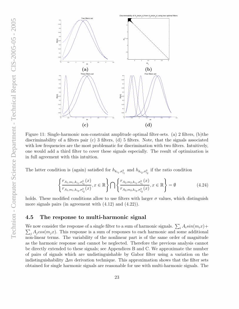
Figure 11: Single-harmonic non-constraint amplitude optimal filter-sets. (a) 2 filters, (b)thediscriminability of a filters pair (c) 3 filters, (d) 5 filters. Note, that the signals associatedwith low frequencies are the most problematic for discrimination with two filters. Intuitively,one would add a third filter to cover these signals especially. The result of optimization isin full agreement with this intuition.

The latter condition is (again) satisfied for hki1,σ2

i1and hki2

,σ2i2

if the ratio condition

{

rA1,m1,ki1,σ2

i1(x)

rA1,m1,ki2,σ2

i2(x)

, x ∈ R

}

⋂

{

rA2,m2,ki1,σ2

i1(x)

rA2,m2,ki2,σ2

i2(x)

, x ∈ R

}

= ∅ (4.24)

holds. These modified conditions allow to use filters with larger σ values, which distinguishmore signals pairs (in agreement with (4.12) and (4.22)).

4.5 The response to multi-harmonic signal

We now consider the response of a single filter to a sum of harmonic signals.∑

i Aisin(mix)+∑

j Ajcos(mjx). This response is a sum of responses to each harmonic and some additionalnon-linear terms. The variability of the nonlinear part is of the same order of magnitudeas the harmonic response and cannot be neglected. Therefore the previous analysis cannotbe directly extended to these signals; see Appendices B and C. We approximate the numberof pairs of signals which are undistinguishable by Gabor filter using a variation on theindistinguishability ∆m derivation technique. This approximation shows that the filter setsobtained for single harmonic signals are reasonable for use with multi-harmonic signals. The

23

Tec

hnio

n -

Com

pute

r Sc

ienc

e D

epar

tmen

t - T

echn

ical

Rep

ort

CIS

-200

5-05

- 2

005

approximations in this section are much rougher then in previous sections. Therefore all thederivations for the multi-harmonic signals should be considered only as supporting evidencesfor suggested filter set and not as exact calculations.

4.5.1 Single filter response to dual-harmonic signal

Consider first a complex Gabor filter hk(x) = 1√2πσ2

e−x2

2σ2 +ikx, and a signal g ~A,~m(x) =

Asin(m1x) + Bsin(m2x) or g ~A,~m(x) = Asin(m1x) + Bcos(m2x). It can be shown (seeAppendix B) that the filter response is bounded with:

Ae−(k2+m2

1)σ2

2 ch(km1σ2) + Be

−(k2+m22)σ2

2 ch(km2σ2)

≥ r ~A,~m,k,σ2(x) ≥ (4.25)∣

∣

∣

∣

Ae−(k2+m2

1)σ2

2 sh(km1σ2) − Be

−(k2+m22)σ2

2 sh(km2σ2)

∣

∣

∣

∣

For large σ, sh(kmσ2) ≃ ch(kmσ2) ≃ ekmσ2the inequality may be rewritten in even simpler

form:

Ae−(k−m1)2σ2

2 + Be−(k−m2)2σ2

2 ≥ 2r ~A,~m,k,σ2(x) ≥∣

∣

∣

∣

Ae−(k−m1)2σ2

2 − Be−(k−m2)2σ2

2

∣

∣

∣

∣

(4.26)

and without loss of generality we can assume that for some A, B, m1, m2

Ae−(k−m1)2σ2

2 ≥ Be−(k−m2)2σ2

2 (4.27)

and refer to m1 as the signal’s primary frequency. Therefore

r ~A,~m,k,σ2 = A2e

−(k−m1)2σ2

2

∆r ~A,~m,k,σ2 = Be−(k−m2)2σ2

2 (4.28)

Note, that the variability is now proportional to the highest response for the single sine caseand depends on other variables than the median response magnitude..

Note that according to our approximation, (B, m2) specifies only the responses variability,therefore changing them does not make the signal distinguishable in all cases. For example,(A, m1, B, m2) is not distinguishable from (A, m1, B

′, m′2) for any B′, m′

2. Following thederivations above (section 4.4, 4.3.3), the interval of indistinguishable signals with primaryfrequency m′

1 6= m1 is

∆m ∼=∆r ~A,k,~m,σ2∣

∣

∣

∂r ~A,k,~m,σ2

∂m1

∣

∣

∣

=Be

−(k−m2)2σ2

2

A2e

−(k−m1)2σ2

2 |k − m1| σ2.

The condition (4.27) is equivalent to

Be−(k−m2)2σ2

2

Ae−(k−m1)2σ2

2

≤ 1,

24

Tec

hnio

n -

Com

pute

r Sc

ienc

e D

epar

tmen

t - T

echn

ical

Rep

ort

CIS

-200

5-05

- 2

005

implying that the indiscriminability measure is roughly bounded with:

∆m ≤ 2

|k − m1|σ2. (4.29)

Note that this expression relies on the approximation of the response by the approximatedbounds center value and variability. Still the expression provide useful intuition: the boundon ∆m decreases when m1 is distant from k, and substantially increases when it becomescloser to k. Therefore, given a pair of signals where both frequencies m1 of both signalsare close to filter’s frequency k, it is less likely that the filter would separate these signals(although it still may happen for some values of A, B, m2 ).

0 0.5 1 1.5 2 2.5 3 3.50

0.05

0.1

0.15

0.2

0.25

0.3

0.35

0.4

0.45

0.5Optimal Filter Set on Linear Frequency Domain

m

RA

,m,k

i, σ2 i

10−1

100

101

0

0.05

0.1

0.15

0.2

0.25

0.3

0.35

0.4

0.45

0.5Optimal Filter Set on Linear Frequency Domain

m

RA

,m,k

i, σ2 i

(a) (b)

0 0.5 1 1.5 2 2.5 3 3.50

0.05

0.1

0.15

0.2

0.25

0.3

0.35

0.4

0.45

0.5Optimal Filter Set on Logarithmic Frequency Domain

m

RA

,m,k

i,σ2 i

10−1

100

101

0

0.05

0.1

0.15

0.2

0.25

0.3

0.35

0.4

0.45

0.5Optimal Filter Set on Logarithmic Frequency Domain

m

RA

,m,k

i,σ2 i

(c) (d)

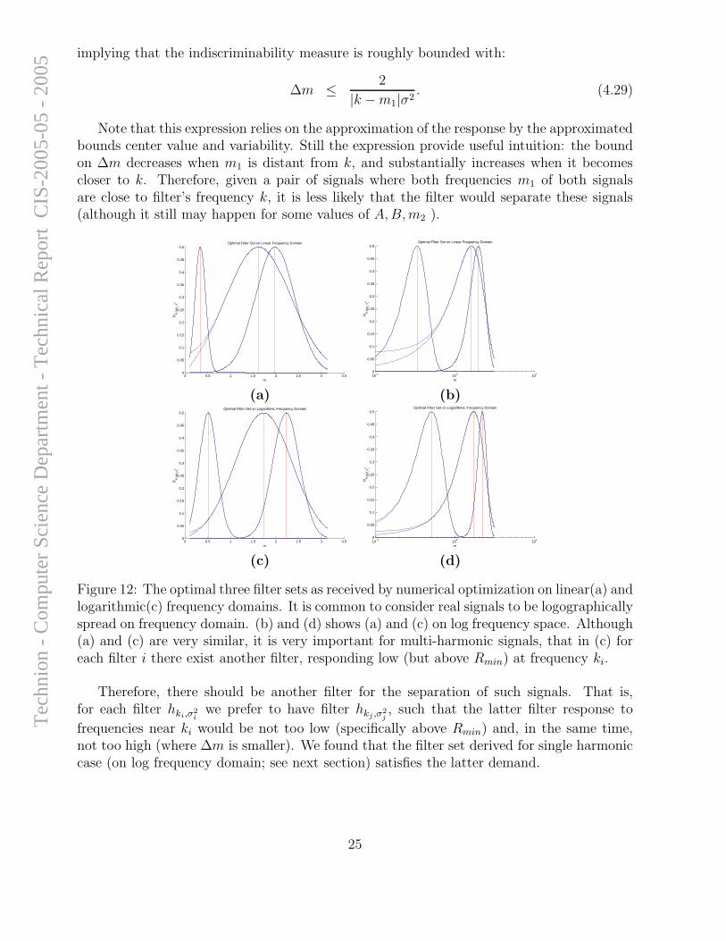
Figure 12: The optimal three filter sets as received by numerical optimization on linear(a) andlogarithmic(c) frequency domains. It is common to consider real signals to be logographicallyspread on frequency domain. (b) and (d) shows (a) and (c) on log frequency space. Although(a) and (c) are very similar, it is very important for multi-harmonic signals, that in (c) foreach filter i there exist another filter, responding low (but above Rmin) at frequency ki.

Therefore, there should be another filter for the separation of such signals. That is,for each filter hki,σ

2i

we prefer to have filter hkj ,σ2j, such that the latter filter response to

frequencies near ki would be not too low (specifically above Rmin) and, in the same time,not too high (where ∆m is smaller). We found that the filter set derived for single harmoniccase (on log frequency domain; see next section) satisfies the latter demand.

25

Tec

hnio

n -

Com

pute

r Sc

ienc

e D

epar

tmen

t - T

echn

ical

Rep

ort

CIS

-200

5-05

- 2

005

4.5.2 Multi-harmonic signals

It is shown in Appendix C that the filter design considerations in the case of multi-harmonicsignals are similar to those of the dual-harmonic case. The filters are likely to have difficultieswith recognition of signals, some of which frequencies are close to the central frequency of thefilter, as in the case of dual harmonic signals. Therefore, according to the reasons describedfor dual harmonic signals, the filters derived for the single harmonic signals are suitable forall harmonic signals. This conclusion provides some justification to apply the derived singleharmonic filters to the task of segmentation of general textured signals.

26

Tec

hnio

n -

Com

pute

r Sc

ienc

e D

epar

tmen

t - T

echn

ical

Rep

ort

CIS

-200

5-05

- 2

005

5 Building an optimal filters-set

In previous section we derived expressions for parameters of optimal single filter for discrimi-nating harmonic signals with equal amplitudes. We also shown a semi analytical way to findoptimal filters pair for segmentation of harmonic signals with unconstrained amplitudes. Inthis section we describe the numerical search we performed on the filters’ parameters to sup-port the theoretical conclusions. Making the full search for many filters is computationallyexpensive. We show how to extend the semi-analytical method (developed for finding twofilters set) so that multi-filter set can be found with relatively small complexity.

In order to find the optimal filter-sets we performed a numerical search. For combinationof filters parameters ~k, ~σ2 taken on some hierarchical grid, the value of a discrete version ofQ(~k, ~σ2) was calculated. In the case of single filter segregating harmonic signals with presetamplitudes we calculated Rk,σ2 using (4.3,4.4) and then inserted it into (4.8). In the case ofseveral (2,3,4,5) filters for segmentation of signals with unconstrained amplitudes, (4.20) wasused to for evaluation of Rk,σ2. Note, that the use of (4.20) allowed to evaluate s(mi, mj)without considering actual amplitudes (see claim 1.1).

The frequencies of signal pairs were taken from a 2D uniformly spaced grid in either alinear:

f lini = fmin + i · f lin

step, where f linstep =

fmax − fmin

N

or a logarithmic:

f logi = fmin ·

(

f logstep

)i

, where f logstep = N

√

fmax

fmin

frequency domains. The discrete versions of Q(~k, ~σ2) are defined as:

Qlin =

∑

i,j∈[0...N ] s(flini , f lin

j )

N2(5.1)

Qlog =

∑

i,j∈[0...N ] s(flogi , f log

j )

N2(5.2)

Note that the analytically calculated filters correspond to the linear domain. Optimizingover the logarithmic domain is advantageous because the number of separated frequenciesis preserved with the scaling process, which presents in every vision system. Therefore,the separation power of the filter set doesn’t depend on the distance from the camera tothe object, which is an important property for a filter set. There are also psychophysicalevidences that logarithmic domain is consistent with human perception. The receptive-fieldprofiles of simple cells in the striate cortex have an octave-like order of frequencies, which isa way to cover uniformly the logarithmic domain. The results for the logarithmic domainwere somewhat different. For each type of frequency domains we tested two [fmin, fmax]bounds - [0.1, 2.82] and [0.1, 3.14]. 2

2The considered fmax values are associated with the Nyquist frequency specified by the sampling of theimage, and fmin is to be the frequency associated with a wavelength equal to the maximal detectable texturepatch size, which we have set to 20π

27

Tec

hnio

n -

Com

pute

r Sc

ienc

e D

epar

tmen

t - T

echn

ical

Rep

ort

CIS

-200

5-05

- 2

005

5.1 The technique of the numerical search

We searched for optimal filters’ parameters for filter sets of one filter for preset amplitudesignals and 2 to 5 filters for unconstrained amplitudes signals. Since each signal is describedby its frequency m (2 parameters in each search) and each filter is described by two parame-ters k and σ2 (2,4,6,8 or 10 parameters), the complexity of search for the optimal filters setvaried between O(n4) to O(n12), where n is the number of possible values tested for each ofthe parameters. This may be computationally hard. Therefore we used a hierarchical, gridbased, search.

We started with a widely spaced grid of k and σ2 parameters (10 values of each) andexamined every combination of them against a rough frequencies m grid (305× 305 values).For the filters’ parameters with best Q measure we defined a finer grid around each parameter.We took the optimal value and its two neighbors from the coarse grid and added two equallyspaced values between them (see figure 13). We repeated the search on the received finer gridsand repeated the grid redefinition around the optimal values. We repeated this operationuntil the resolutions of filter parameter grids where of the same order as the resolution ofthe frequencies grid.

y y y

6XXXXXXy������:

coarse grid

i i?������9

XXXXXXz����

HHHj

fine grid

Figure 13: Converting coarse grid to fine

In the case when several different sets of filter parameters give the same Q value, weincreased the resolution of signals grid and repeated the calculations for these sets, tryingto find the best one.

5.2 Signals with equal amplitudes

In section 4.2 we derived theoretically a single optimal filter for segregation of harmonicsignals with equal amplitudes (4.17). This derivation was numerically confirmed with asearch over k parameter in [fmin, fmax] domains and over σ2 parameter in [1,100] range.Each signal pair was examined vs. (4.9) test and the k, σ2 parameters which maximizedQ(k, σ2) were chosen as the optimal filter.

We considered different values of Rmin parameter between 5% and 20% of Rmax. We foundthat while the optimal ki was not sensitive to Rmin, the σ2

i was. For small Rmin values theoptimized parameters are very similar to the theoretical ones; see (4.17). For bigger valuesof Rmin it is preferred to decrease the filter’s coverage and to give up the discrimination ofsome signal pairs in order to increase the segregation rate for the remaining ones.

5.3 Extension of the semi-analytical method for filter sets of threeand more filters for signals with unconstrained amplitudes

In section 4.3 we proposed a semi-analytic method for receiving the approximately optimalfilter parameters for segregation of single harmonic signals with unconstrained amplitudes.

28

Tec

hnio

n -

Com

pute

r Sc

ienc

e D

epar

tmen

t - T

echn

ical

Rep

ort

CIS

-200

5-05

- 2

005

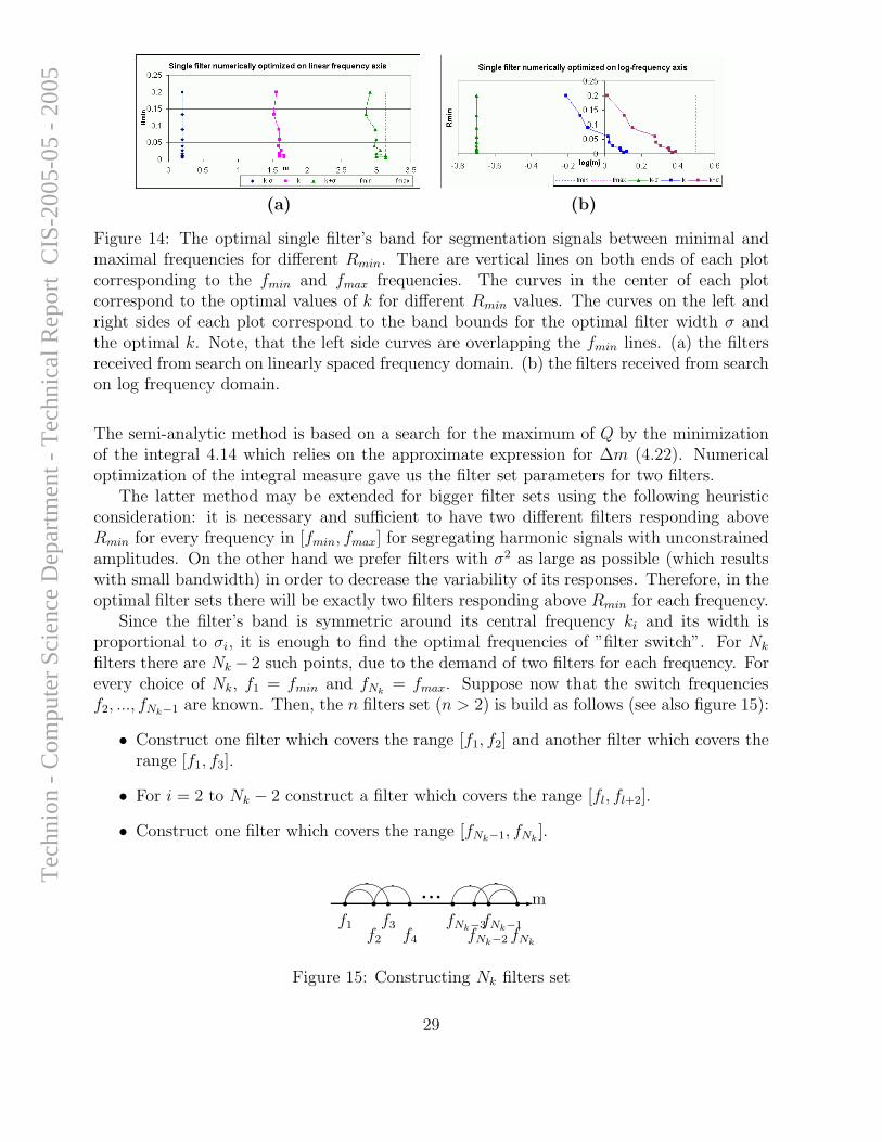
(a) (b)

Figure 14: The optimal single filter’s band for segmentation signals between minimal andmaximal frequencies for different Rmin. There are vertical lines on both ends of each plotcorresponding to the fmin and fmax frequencies. The curves in the center of each plotcorrespond to the optimal values of k for different Rmin values. The curves on the left andright sides of each plot correspond to the band bounds for the optimal filter width σ andthe optimal k. Note, that the left side curves are overlapping the fmin lines. (a) the filtersreceived from search on linearly spaced frequency domain. (b) the filters received from searchon log frequency domain.

The semi-analytic method is based on a search for the maximum of Q by the minimizationof the integral 4.14 which relies on the approximate expression for ∆m (4.22). Numericaloptimization of the integral measure gave us the filter set parameters for two filters.

The latter method may be extended for bigger filter sets using the following heuristicconsideration: it is necessary and sufficient to have two different filters responding aboveRmin for every frequency in [fmin, fmax] for segregating harmonic signals with unconstrainedamplitudes. On the other hand we prefer filters with σ2 as large as possible (which resultswith small bandwidth) in order to decrease the variability of its responses. Therefore, in theoptimal filter sets there will be exactly two filters responding above Rmin for each frequency.

Since the filter’s band is symmetric around its central frequency ki and its width isproportional to σi, it is enough to find the optimal frequencies of ”filter switch”. For Nk

filters there are Nk − 2 such points, due to the demand of two filters for each frequency. Forevery choice of Nk, f1 = fmin and fNk

= fmax. Suppose now that the switch frequenciesf2, ..., fNk−1 are known. Then, the n filters set (n > 2) is build as follows (see also figure 15):

• Construct one filter which covers the range [f1, f2] and another filter which covers therange [f1, f3].

• For i = 2 to Nk − 2 construct a filter which covers the range [fl, fl+2].

• Construct one filter which covers the range [fNk−1, fNk].

-m��� ��� ��� ���

q q qr

f1

r

f2

r

f3

r

f4

r

fNk−3

r

fNk−2

r

fNk−1

r

fNk

Figure 15: Constructing Nk filters set

29

Tec

hnio

n -

Com

pute

r Sc

ienc

e D

epar

tmen

t - T

echn

ical

Rep

ort

CIS

-200

5-05

- 2

005

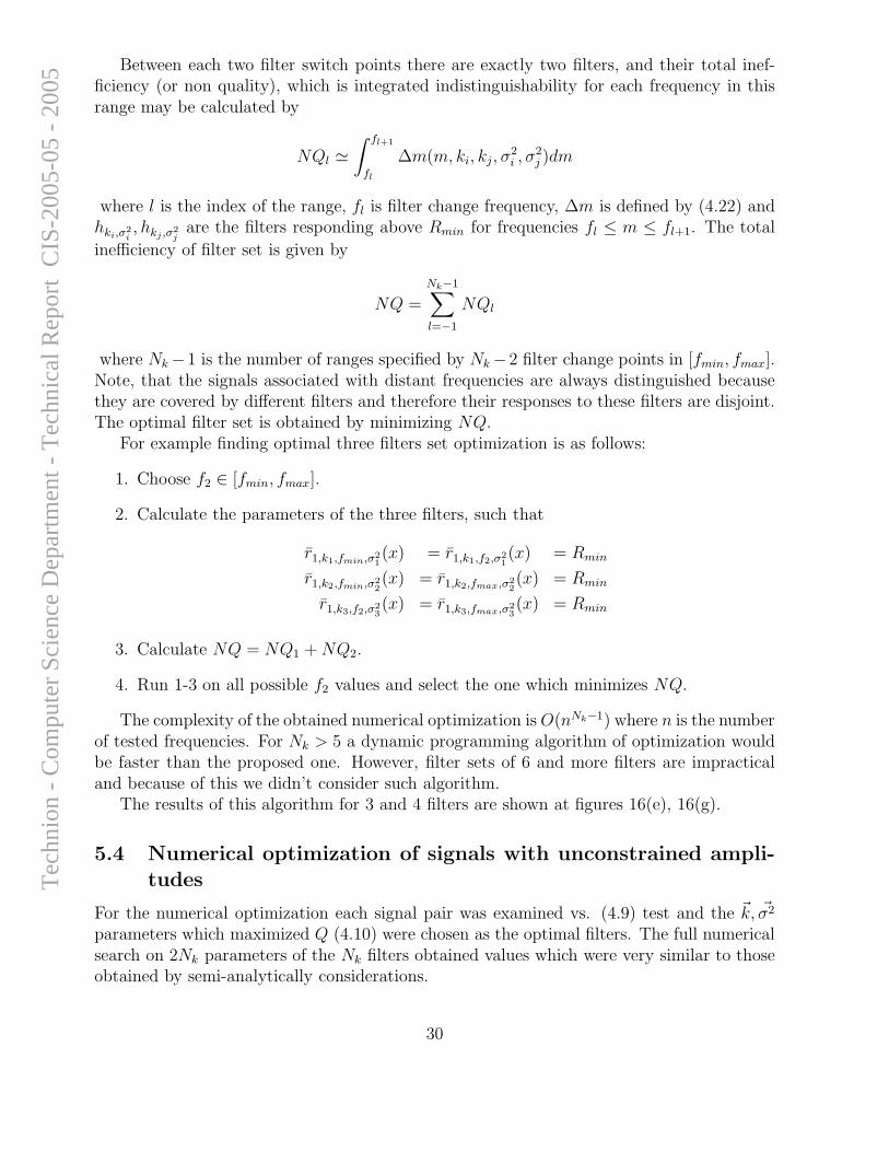
Between each two filter switch points there are exactly two filters, and their total inef-ficiency (or non quality), which is integrated indistinguishability for each frequency in thisrange may be calculated by

NQl ≃∫ fl+1

fl

∆m(m, ki, kj, σ2i , σ

2j )dm

where l is the index of the range, fl is filter change frequency, ∆m is defined by (4.22) andhki,σ

2i, hkj ,σ2

jare the filters responding above Rmin for frequencies fl ≤ m ≤ fl+1. The total

inefficiency of filter set is given by

NQ =

Nk−1∑

l=−1

NQl

where Nk −1 is the number of ranges specified by Nk −2 filter change points in [fmin, fmax].Note, that the signals associated with distant frequencies are always distinguished becausethey are covered by different filters and therefore their responses to these filters are disjoint.The optimal filter set is obtained by minimizing NQ.

For example finding optimal three filters set optimization is as follows:

1. Choose f2 ∈ [fmin, fmax].

2. Calculate the parameters of the three filters, such that

r1,k1,fmin,σ21(x) = r1,k1,f2,σ2

1(x) = Rmin

r1,k2,fmin,σ22(x) = r1,k2,fmax,σ2

2(x) = Rmin

r1,k3,f2,σ23(x) = r1,k3,fmax,σ2

3(x) = Rmin

3. Calculate NQ = NQ1 + NQ2.

4. Run 1-3 on all possible f2 values and select the one which minimizes NQ.

The complexity of the obtained numerical optimization is O(nNk−1) where n is the numberof tested frequencies. For Nk > 5 a dynamic programming algorithm of optimization wouldbe faster than the proposed one. However, filter sets of 6 and more filters are impracticaland because of this we didn’t consider such algorithm.

The results of this algorithm for 3 and 4 filters are shown at figures 16(e), 16(g).

5.4 Numerical optimization of signals with unconstrained ampli-tudes

For the numerical optimization each signal pair was examined vs. (4.9) test and the ~k, ~σ2

parameters which maximized Q (4.10) were chosen as the optimal filters. The full numericalsearch on 2Nk parameters of the Nk filters obtained values which were very similar to thoseobtained by semi-analytically considerations.

30

Tec

hnio

n -

Com

pute

r Sc

ienc

e D

epar

tmen

t - T

echn

ical

Rep

ort

CIS

-200

5-05

- 2

005

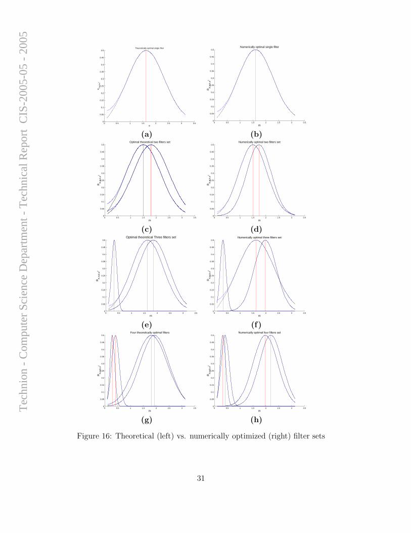
0 0.5 1 1.5 2 2.5 3 3.50

0.05

0.1

0.15

0.2

0.25

0.3

0.35

0.4

0.45

0.5Theoretically optimal single filter

m

RA

,m,k

,σ2

0 0.5 1 1.5 2 2.5 3 3.50

0.05

0.1

0.15

0.2

0.25

0.3

0.35

0.4

0.45

0.5Numerically optimal single filter

m

RA

,m,k

,σ2

(a) (b)

0 0.5 1 1.5 2 2.5 3 3.50

0.05

0.1

0.15

0.2

0.25

0.3

0.35

0.4

0.45

0.5Optimal theoretical two filters set

m

RA

,m,k

,σ2

0 0.5 1 1.5 2 2.5 3 3.50

0.05

0.1

0.15

0.2

0.25

0.3

0.35

0.4

0.45

0.5Numerically optimal two filters set

m

RA

,m,k

,σ2

(c) (d)

0 0.5 1 1.5 2 2.5 3 3.50

0.05

0.1

0.15

0.2

0.25

0.3

0.35

0.4

0.45

0.5Optimal theoretical Three filters set

m

RA

,m,k

,σ2

0 0.5 1 1.5 2 2.5 3 3.50

0.05

0.1

0.15

0.2

0.25

0.3

0.35

0.4

0.45

0.5Numerically optimal three filters set

m

RA

,m,k

,σ2

(e) (f)

0 0.5 1 1.5 2 2.5 3 3.50

0.05

0.1

0.15

0.2

0.25

0.3

0.35

0.4

0.45

0.5Four theoretically optimal filters

m

RA

,m,k

,σ2

0 0.5 1 1.5 2 2.5 3 3.50

0.05

0.1

0.15

0.2

0.25

0.3

0.35

0.4

0.45

0.5Numerically optimal four filters set

m

RA

,m,k

,σ2

(g) (h)

Figure 16: Theoretical (left) vs. numerically optimized (right) filter sets

31

Tec

hnio

n -

Com

pute

r Sc

ienc

e D

epar

tmen

t - T

echn

ical

Rep

ort

CIS

-200

5-05

- 2

005

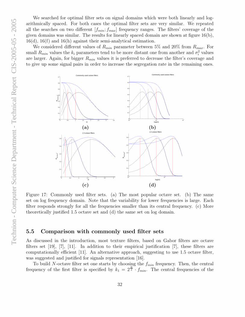
We searched for optimal filter sets on signal domains which were both linearly and log-arithmically spaced. For both cases the optimal filter sets are very similar. We repeatedall the searches on two different [fmin; fmax] frequency ranges. The filters’ coverage of thegiven domains was similar. The results for linearly spaced domain are shown at figure 16(b),16(d), 16(f) and 16(h) against their semi-analytical estimation.

We considered different values of Rmin parameter between 5% and 20% from Rmax. Forsmall Rmin values the ki parameters tend to be more distant one from another and σ2

i valuesare larger. Again, for bigger Rmin values it is preferred to decrease the filter’s coverage andto give up some signal pairs in order to increase the segregation rate in the remaining ones.

0 0.5 1 1.5 2 2.5 3 3.50

0.1

0.2

0.3

0.4

0.5

0.6

0.7Commonly used octave filters

m

RA

,m,k

,σ2

10−1

100

101

0

0.1

0.2

0.3

0.4

0.5

0.6

0.7Commonly used octave filters

log(m)

(a) (b)

0 0.5 1 1.5 2 2.5 30

0.1

0.2

0.3

0.4

0.5

1.5 octave filters

m

RA

,m,k

,σ2

10−1

100

0

0.1

0.2

0.3

0.4

0.5

1.5 octave filters

log(m)

RA

,m,k

,σ2

(c) (d)

Figure 17: Commonly used filter sets. (a) The most popular octave set. (b) The sameset on log frequency domain. Note that the variability for lower frequencies is large. Eachfilter responds strongly for all the frequencies smaller than its central frequency. (c) Moretheoretically justified 1.5 octave set and (d) the same set on log domain.

5.5 Comparison with commonly used filter sets

As discussed in the introduction, most texture filters, based on Gabor filters are octavefilters set [19], [7], [11]. In addition to their empirical justification [7], these filters arecomputationally efficient [11]. An alternative approach, suggesting to use 1.5 octave filter,was suggested and justified for signals representation [16].

To build N -octave filter set one starts by choosing the fmin frequency. Then, the centralfrequency of the first filter is specified by k1 = 2

N2 · fmin. The central frequencies of the

32

Tec

hnio

n -

Com

pute

r Sc

ienc

e D

epar

tmen

t - T

echn

ical

Rep

ort

CIS

-200

5-05

- 2

005

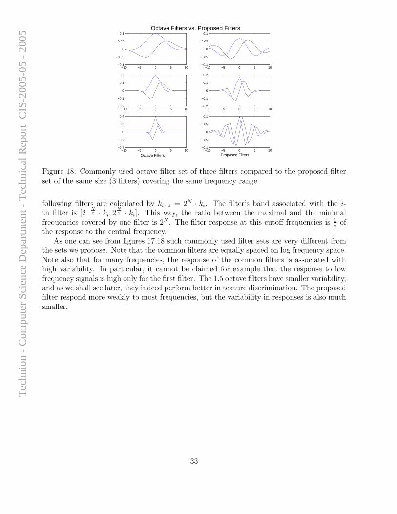
−10 −5 0 5 10−0.1

−0.05

0

0.05

0.1

−10 −5 0 5 10−0.2

−0.1

0

0.1

0.2

−10 −5 0 5 10−0.4

−0.2

0

0.2

0.4

−10 −5 0 5 10−0.2

−0.1

0

0.1

0.2

−10 −5 0 5 10−0.1

−0.05

0

0.05

0.1

−10 −5 0 5 10−0.1

−0.05

0

0.05

0.1Octave Filters vs. Proposed Filters

Octave Filters Proposed Filters

Figure 18: Commonly used octave filter set of three filters compared to the proposed filterset of the same size (3 filters) covering the same frequency range.

following filters are calculated by ki+1 = 2N · ki. The filter’s band associated with the i-th filter is [2−

N2 · ki; 2

N2 · ki]. This way, the ratio between the maximal and the minimal

frequencies covered by one filter is 2N . The filter response at this cutoff frequencies is 1e

ofthe response to the central frequency.

As one can see from figures 17,18 such commonly used filter sets are very different fromthe sets we propose. Note that the common filters are equally spaced on log frequency space.Note also that for many frequencies, the response of the common filters is associated withhigh variability. In particular, it cannot be claimed for example that the response to lowfrequency signals is high only for the first filter. The 1.5 octave filters have smaller variability,and as we shall see later, they indeed perform better in texture discrimination. The proposedfilter respond more weakly to most frequencies, but the variability in responses is also muchsmaller.

33

Tec

hnio

n -

Com

pute

r Sc

ienc

e D

epar

tmen

t - T

echn

ical

Rep

ort

CIS

-200

5-05

- 2

005

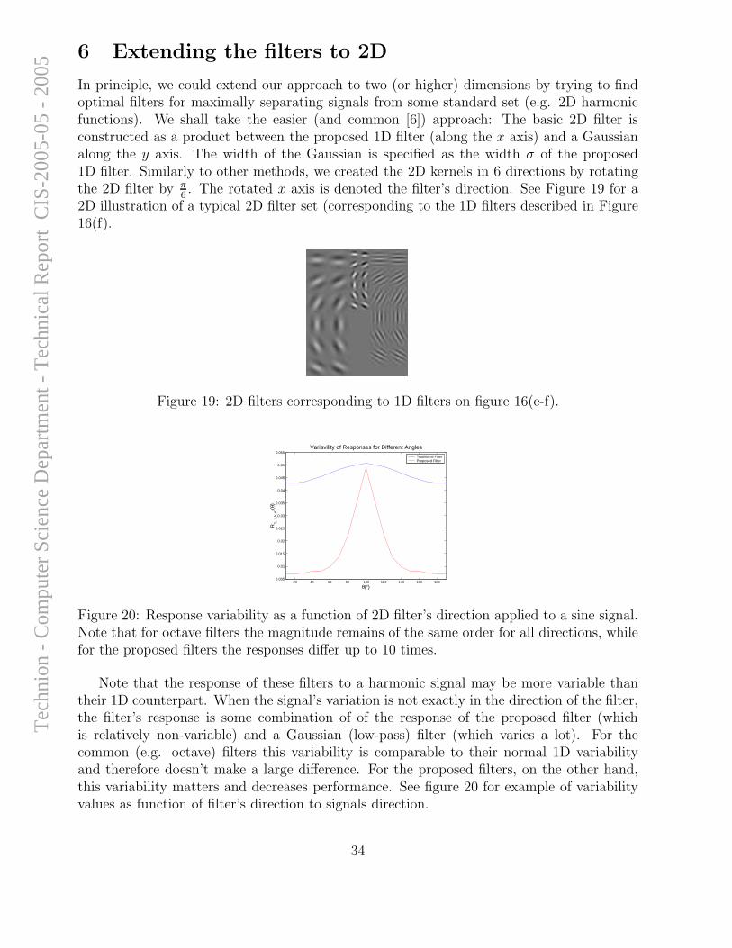
6 Extending the filters to 2D

In principle, we could extend our approach to two (or higher) dimensions by trying to findoptimal filters for maximally separating signals from some standard set (e.g. 2D harmonicfunctions). We shall take the easier (and common [6]) approach: The basic 2D filter isconstructed as a product between the proposed 1D filter (along the x axis) and a Gaussianalong the y axis. The width of the Gaussian is specified as the width σ of the proposed1D filter. Similarly to other methods, we created the 2D kernels in 6 directions by rotatingthe 2D filter by π

6. The rotated x axis is denoted the filter’s direction. See Figure 19 for a

2D illustration of a typical 2D filter set (corresponding to the 1D filters described in Figure16(f).

Figure 19: 2D filters corresponding to 1D filters on figure 16(e-f).

20 40 60 80 100 120 140 160 1800.005

0.01

0.015

0.02

0.025

0.03

0.035

0.04

0.045

0.05

0.055Variavility of Responses for Different Angles

θ(°)

R1,

.1,k

,σ2(

θ)

Traditional FilterProposed Filter

Figure 20: Response variability as a function of 2D filter’s direction applied to a sine signal.Note that for octave filters the magnitude remains of the same order for all directions, whilefor the proposed filters the responses differ up to 10 times.

Note that the response of these filters to a harmonic signal may be more variable thantheir 1D counterpart. When the signal’s variation is not exactly in the direction of the filter,the filter’s response is some combination of of the response of the proposed filter (whichis relatively non-variable) and a Gaussian (low-pass) filter (which varies a lot). For thecommon (e.g. octave) filters this variability is comparable to their normal 1D variabilityand therefore doesn’t make a large difference. For the proposed filters, on the other hand,this variability matters and decreases performance. See figure 20 for example of variabilityvalues as function of filter’s direction to signals direction.

34

Tec

hnio

n -

Com

pute

r Sc

ienc

e D

epar

tmen

t - T

echn

ical

Rep

ort

CIS

-200

5-05

- 2

005

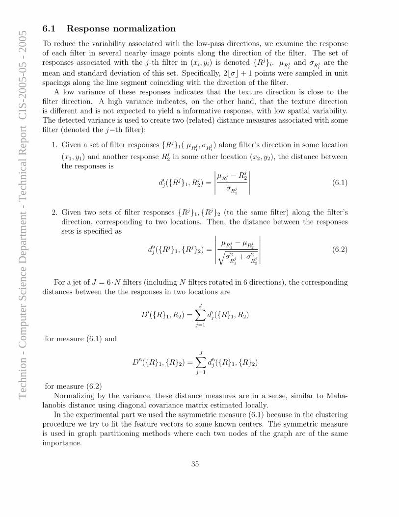
6.1 Response normalization

To reduce the variability associated with the low-pass directions, we examine the responseof each filter in several nearby image points along the direction of the filter. The set ofresponses associated with the j-th filter in (xi, yi) is denoted {Rj}i. µ

Rji

and σR

ji

are the

mean and standard deviation of this set. Specifically, 2⌊σ⌋ + 1 points were sampled in unitspacings along the line segment coinciding with the direction of the filter.

A low variance of these responses indicates that the texture direction is close to thefilter direction. A high variance indicates, on the other hand, that the texture directionis different and is not expected to yield a informative response, with low spatial variability.The detected variance is used to create two (related) distance measures associated with somefilter (denoted the j−th filter):

1. Given a set of filter responses {Rj}1( µR

j1, σ

Rj1) along filter’s direction in some location

(x1, y1) and another response Rj2 in some other location (x2, y2), the distance between

the responses is

d8

j({Rj}1, Rj2) =

∣

∣

∣

∣

∣

µR

j1− Rj

2

σR

j1

∣

∣

∣

∣

∣

(6.1)

2. Given two sets of filter responses {Rj}1, {Rj}2 (to the same filter) along the filter’sdirection, corresponding to two locations. Then, the distance between the responsessets is specified as

d88

j ({Rj}1, {Rj}2) =

∣

∣

∣

∣

∣

∣

µR

j1− µ

Rj2

√

σ2R

j1

+ σ2R

j2

∣

∣

∣

∣

∣

∣

(6.2)

For a jet of J = 6·N filters (including N filters rotated in 6 directions), the correspondingdistances between the the responses in two locations are

D8({R}1, R2) =J∑

j=1

d8

j({R}1, R2)

for measure (6.1) and

D88({R}1, {R}2) =J∑

j=1

d88

j ({R}1, {R}2)

for measure (6.2)Normalizing by the variance, these distance measures are in a sense, similar to Maha-

lanobis distance using diagonal covariance matrix estimated locally.In the experimental part we used the asymmetric measure (6.1) because in the clustering

procedure we try to fit the feature vectors to some known centers. The symmetric measureis used in graph partitioning methods where each two nodes of the graph are of the sameimportance.

35

Tec

hnio

n -

Com

pute

r Sc

ienc

e D

epar

tmen

t - T

echn

ical

Rep

ort

CIS

-200

5-05

- 2

005

7 Experiments

7.1 Testing texture descriptors

Retrieval test - This test, built around the image retrieval tasks. A (typically large) set ofimages containing various textures is available. In a query, a texture patch is given, andthe images with a similar texture are sought. A query is successful if an image with the(subjectively judge) same texture is found to be one of the k most similar (accordingto the descriptor) images [24], or if all the images associated with this texture in thedatabase are found [29]. It is sufficient to find the image and no specification wherethe query texture is present in the image is required.

Segmentation test - In this test, an image with several textured regions present in it, isgiven, and the algorithm needs to correctly specify these regions [19]. The algorithmmay involve texture descriptor as well as spatial considerations and is essentially aclustering procedure. The texture descriptor ability to provide an effective distancemeasure is tested. Simpler segmentations tests involve semi synthetic images composedof tiles where every tile contains some (synthetic or real) texture. Harder tests involvereal images, containing textured objects, where the texture is influenced by say 3Dstructure, or object pose.

Focusing on the issue of descriptor stability under translation, which is important mostlyfor segmentation, we tested the proposed descriptors using the segmentation test. Textureschanges associated with 3D structure and pose correspond to scaling and shear and arebeyond the scope of this work.

Moreover, spatial considerations such as region size, and preference to texture continuitywere not used as well. This is done so that these considerations, or a segmentation algorithmrelying on them, would not mask the differences associated with the usage of different filtersets. Our experiments basically test the texture distance between different textures (and itsstability) compared with a similar distance within the same texture.

We tested the discrimination power of the proposed filter-sets as well as several other,commonly used, filter-sets, using both the common L2 metric and the two new distancemeasures proposed above. The experiments were done with synthetic sine images (biasedfor our filters) and with the popular Brodatz textures.

Our results indicate that the proposed filter sets perform significantly better than thecommonly used methods.

In aspect of retrieval test, we compare the proposed filters versus common octave filtersset using the texture recognition algorithm by Varma and Zisserman [28]. The algorithmis implemented exactly as described by the authors and tested with the original and theproposed filter sets on the original database. The results for the algorithm parametersreported in the article are similar for both filter sets. However the proposed filters obtainvery close results using much more compact texture representation (smaller runtime), unlikethe octave filters.

36

Tec

hnio

n -

Com

pute

r Sc

ienc

e D

epar

tmen

t - T

echn

ical

Rep

ort

CIS

-200

5-05

- 2

005

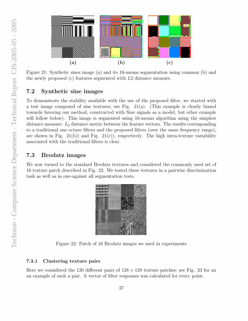
(a) (b) (c)

Figure 21: Synthetic sines image (a) and its 16-means segmentation using common (b) andthe newly proposed (c) features segmented with L2 distance measure.

7.2 Synthetic sine images

To demonstrate the stability available with the use of the proposed filter, we started witha test image composed of sine textures; see Fig. 21(a). (This example is clearly biasedtowards favoring our method, constructed with Sine signals as a model, but other examplewill follow below). This image is segmented using 16-means algorithm using the simplestdistance measure: L2 distance metric between the feature vectors. The results correspondingto a traditional one octave filters and the proposed filters (over the same frequency range),are shown in Fig. 21(b)) and Fig. 21(c)), respectively. The high intra-texture variabilityassociated with the traditional filters is clear.

7.3 Brodatz images

We now turned to the standard Brodatz textures and considered the commonly used set of16 texture patch described in Fig. 22. We tested these textures in a pairwise discriminationtask as well as in one-against all segmentation tests.

Figure 22: Patch of 16 Brodatz images we used in experiments

7.3.1 Clustering texture pairs

Here we considered the 120 different pairs of 128 × 128 texture patches; see Fig. 23 for anan example of such a pair. A vector of filter responses was calculated for every point.

37

Tec

hnio

n -

Com

pute

r Sc

ienc

e D

epar

tmen

t - T

echn

ical

Rep

ort

CIS

-200

5-05

- 2

005

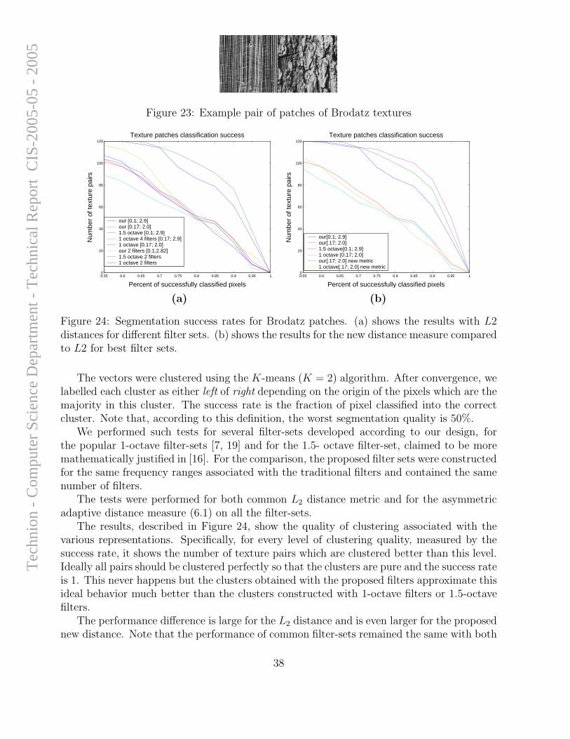
Figure 23: Example pair of patches of Brodatz textures

0.55 0.6 0.65 0.7 0.75 0.8 0.85 0.9 0.95 10

20

40

60

80

100

120Texture patches classification success

Percent of successfully classified pixels

Num

ber

of te

xtur

e pa

irs

our [0.1; 2.9]our [0.17; 2.0]1.5 octave [0.1; 2.9]1 octave 4 filters [0.17; 2.9]1 octave [0.17; 2.0]our 2 filters [0.1;2.82]1.5 octave 2 filters1 octave 2 filters

0.55 0.6 0.65 0.7 0.75 0.8 0.85 0.9 0.95 10

20

40

60

80

100

120Texture patches classification success

Percent of successfully classified pixelsN

umbe

r of

text

ure

pairs

our[0.1; 2.9]our[.17; 2.0]1.5 octave[0.1; 2.9]1 octave [0.17; 2.0]our[.17; 2.0] new metric1 octave[.17; 2.0] new metric

(a) (b)

Figure 24: Segmentation success rates for Brodatz patches. (a) shows the results with L2distances for different filter sets. (b) shows the results for the new distance measure comparedto L2 for best filter sets.

The vectors were clustered using the K-means (K = 2) algorithm. After convergence, welabelled each cluster as either left of right depending on the origin of the pixels which are themajority in this cluster. The success rate is the fraction of pixel classified into the correctcluster. Note that, according to this definition, the worst segmentation quality is 50%.

We performed such tests for several filter-sets developed according to our design, forthe popular 1-octave filter-sets [7, 19] and for the 1.5- octave filter-set, claimed to be moremathematically justified in [16]. For the comparison, the proposed filter sets were constructedfor the same frequency ranges associated with the traditional filters and contained the samenumber of filters.

The tests were performed for both common L2 distance metric and for the asymmetricadaptive distance measure (6.1) on all the filter-sets.

The results, described in Figure 24, show the quality of clustering associated with thevarious representations. Specifically, for every level of clustering quality, measured by thesuccess rate, it shows the number of texture pairs which are clustered better than this level.Ideally all pairs should be clustered perfectly so that the clusters are pure and the success rateis 1. This never happens but the clusters obtained with the proposed filters approximate thisideal behavior much better than the clusters constructed with 1-octave filters or 1.5-octavefilters.

The performance difference is large for the L2 distance and is even larger for the proposednew distance. Note that the performance of common filter-sets remained the same with both

38

Tec

hnio

n -

Com

pute

r Sc

ienc

e D

epar

tmen

t - T

echn

ical

Rep

ort

CIS

-200

5-05

- 2

005

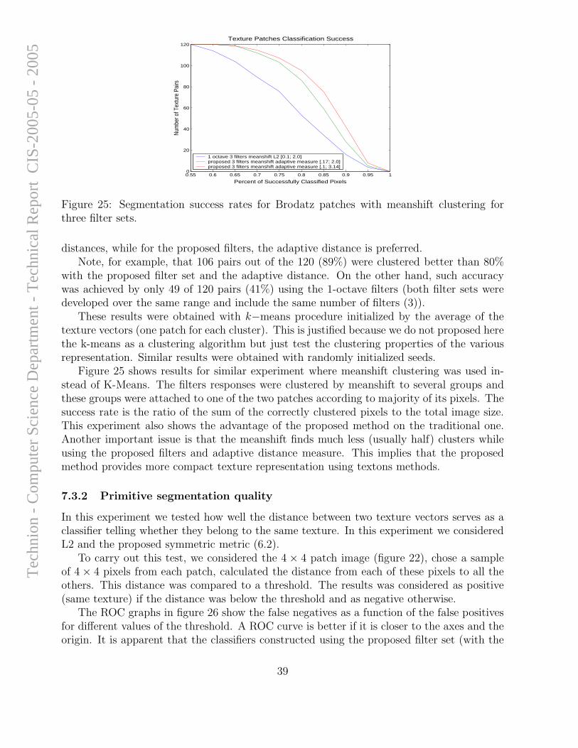
0.55 0.6 0.65 0.7 0.75 0.8 0.85 0.9 0.95 10

20

40

60

80

100

120

Percent of Successfully Classified PixelsN

umbe

r of T

extu

re P

airs

Texture Patches Classification Success

1 octave 3 filters meanshift L2 [0.1; 2.0]proposed 3 filters meanshift adaptive measure [.17; 2.0]proposed 3 filters meanshift adaptive measure [.1; 3.14]

Figure 25: Segmentation success rates for Brodatz patches with meanshift clustering forthree filter sets.

distances, while for the proposed filters, the adaptive distance is preferred.Note, for example, that 106 pairs out of the 120 (89%) were clustered better than 80%

with the proposed filter set and the adaptive distance. On the other hand, such accuracywas achieved by only 49 of 120 pairs (41%) using the 1-octave filters (both filter sets weredeveloped over the same range and include the same number of filters (3)).

These results were obtained with k−means procedure initialized by the average of thetexture vectors (one patch for each cluster). This is justified because we do not proposed herethe k-means as a clustering algorithm but just test the clustering properties of the variousrepresentation. Similar results were obtained with randomly initialized seeds.

Figure 25 shows results for similar experiment where meanshift clustering was used in-stead of K-Means. The filters responses were clustered by meanshift to several groups andthese groups were attached to one of the two patches according to majority of its pixels. Thesuccess rate is the ratio of the sum of the correctly clustered pixels to the total image size.This experiment also shows the advantage of the proposed method on the traditional one.Another important issue is that the meanshift finds much less (usually half) clusters whileusing the proposed filters and adaptive distance measure. This implies that the proposedmethod provides more compact texture representation using textons methods.

7.3.2 Primitive segmentation quality

In this experiment we tested how well the distance between two texture vectors serves as aclassifier telling whether they belong to the same texture. In this experiment we consideredL2 and the proposed symmetric metric (6.2).

To carry out this test, we considered the 4 × 4 patch image (figure 22), chose a sampleof 4 × 4 pixels from each patch, calculated the distance from each of these pixels to all theothers. This distance was compared to a threshold. The results was considered as positive(same texture) if the distance was below the threshold and as negative otherwise.

The ROC graphs in figure 26 show the false negatives as a function of the false positivesfor different values of the threshold. A ROC curve is better if it is closer to the axes and theorigin. It is apparent that the classifiers constructed using the proposed filter set (with the

39

Tec

hnio

n -

Com

pute

r Sc

ienc

e D

epar

tmen

t - T

echn

ical

Rep

ort

CIS

-200

5-05

- 2

005

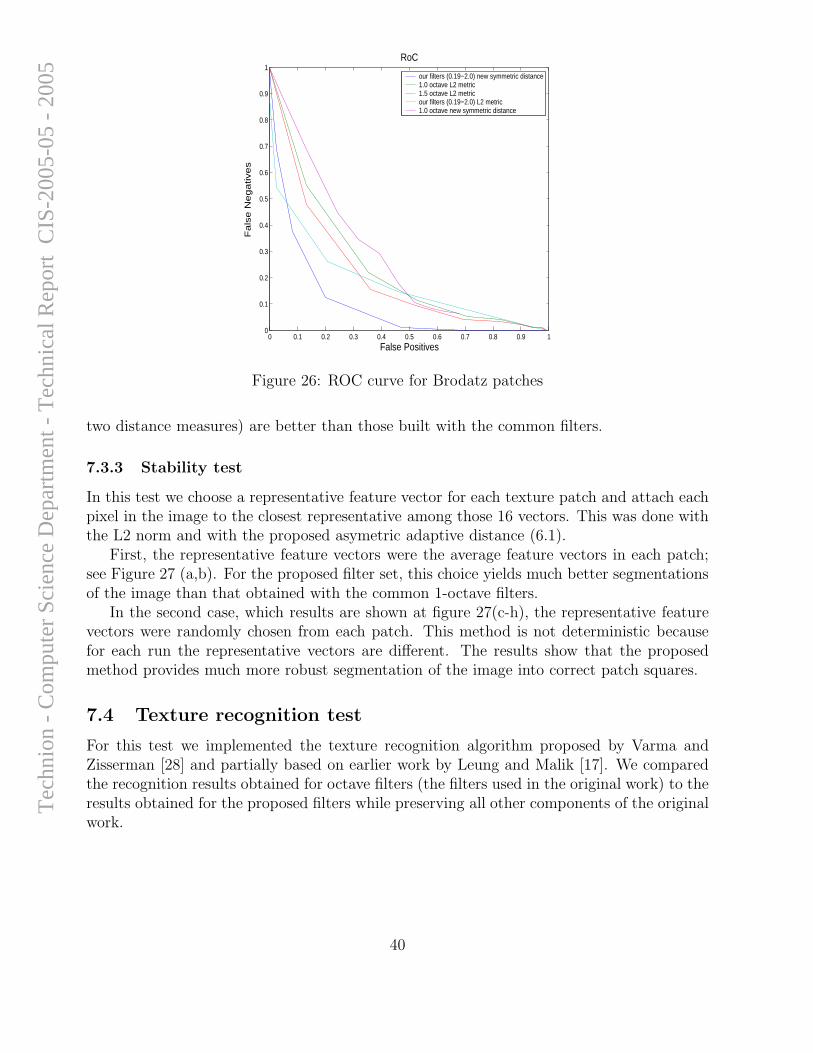
0 0.1 0.2 0.3 0.4 0.5 0.6 0.7 0.8 0.9 10

0.1

0.2

0.3

0.4

0.5

0.6

0.7

0.8

0.9

1RoC

False Positives

Fa

lse

Ne

ga

tive

s

our filters (0.19−2.0) new symmetric distance1.0 octave L2 metric1.5 octave L2 metricour filters (0.19−2.0) L2 metric1.0 octave new symmetric distance

Figure 26: ROC curve for Brodatz patches

two distance measures) are better than those built with the common filters.

7.3.3 Stability test

In this test we choose a representative feature vector for each texture patch and attach eachpixel in the image to the closest representative among those 16 vectors. This was done withthe L2 norm and with the proposed asymetric adaptive distance (6.1).

First, the representative feature vectors were the average feature vectors in each patch;see Figure 27 (a,b). For the proposed filter set, this choice yields much better segmentationsof the image than that obtained with the common 1-octave filters.

In the second case, which results are shown at figure 27(c-h), the representative featurevectors were randomly chosen from each patch. This method is not deterministic becausefor each run the representative vectors are different. The results show that the proposedmethod provides much more robust segmentation of the image into correct patch squares.

7.4 Texture recognition test

For this test we implemented the texture recognition algorithm proposed by Varma andZisserman [28] and partially based on earlier work by Leung and Malik [17]. We comparedthe recognition results obtained for octave filters (the filters used in the original work) to theresults obtained for the proposed filters while preserving all other components of the originalwork.

40

Tec

hnio

n -

Com

pute

r Sc

ienc

e D

epar

tmen

t - T

echn

ical

Rep

ort

CIS

-200

5-05

- 2

005

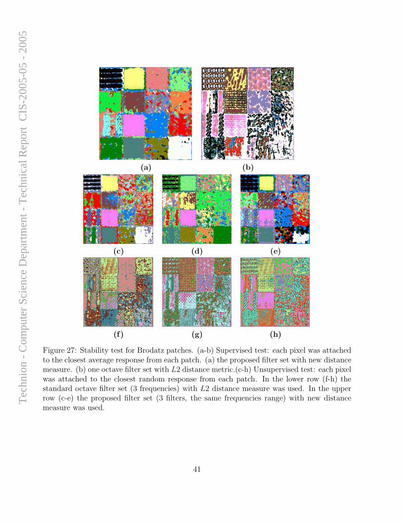
(a) (b)

(c) (d) (e)

(f) (g) (h)

Figure 27: Stability test for Brodatz patches. (a-b) Supervised test: each pixel was attachedto the closest average response from each patch. (a) the proposed filter set with new distancemeasure. (b) one octave filter set with L2 distance metric.(c-h) Unsupervised test: each pixelwas attached to the closest random response from each patch. In the lower row (f-h) thestandard octave filter set (3 frequencies) with L2 distance measure was used. In the upperrow (c-e) the proposed filter set (3 filters, the same frequencies range) with new distancemeasure was used.

41

Tec

hnio

n -

Com

pute

r Sc

ienc

e D

epar

tmen

t - T

echn

ical

Rep

ort

CIS

-200

5-05

- 2

005

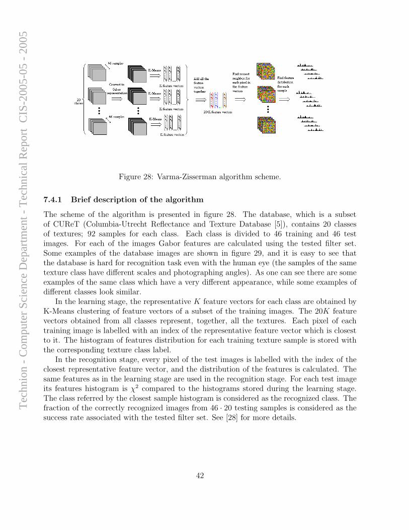
Figure 28: Varma-Zisserman algorithm scheme.

7.4.1 Brief description of the algorithm

The scheme of the algorithm is presented in figure 28. The database, which is a subsetof CUReT (Columbia-Utrecht Reflectance and Texture Database [5]), contains 20 classesof textures; 92 samples for each class. Each class is divided to 46 training and 46 testimages. For each of the images Gabor features are calculated using the tested filter set.Some examples of the database images are shown in figure 29, and it is easy to see thatthe database is hard for recognition task even with the human eye (the samples of the sametexture class have different scales and photographing angles). As one can see there are someexamples of the same class which have a very different appearance, while some examples ofdifferent classes look similar.

In the learning stage, the representative K feature vectors for each class are obtained byK-Means clustering of feature vectors of a subset of the training images. The 20K featurevectors obtained from all classes represent, together, all the textures. Each pixel of eachtraining image is labelled with an index of the representative feature vector which is closestto it. The histogram of features distribution for each training texture sample is stored withthe corresponding texture class label.

In the recognition stage, every pixel of the test images is labelled with the index of theclosest representative feature vector, and the distribution of the features is calculated. Thesame features as in the learning stage are used in the recognition stage. For each test imageits features histogram is χ2 compared to the histograms stored during the learning stage.The class referred by the closest sample histogram is considered as the recognized class. Thefraction of the correctly recognized images from 46 · 20 testing samples is considered as thesuccess rate associated with the tested filter set. See [28] for more details.

42

Tec

hnio

n -

Com

pute

r Sc

ienc

e D

epar

tmen

t - T

echn

ical

Rep

ort

CIS

-200

5-05

- 2

005

(a)

(b)

Figure 29: CUReT images examples. The upper image contain four sample images of thesame class. The bottom image contain four samples from different classes. As one can seesometimes the images in the same class have a very different appearance, while images indifferent classes are very similar

7.4.2 Experiments setup

As first stage we repeated the recognition system exactly as it was proposed in the article[28] and tested it on the same database. The obtained results were similar to those reportedby the authors, thus we concluded that our implementation is correct. We used a variation ofthe filter set denoted RFS in the original work, with the omission of the two isotropic filters.The best result reported by the authors for 20 classes recognition is 98.37%; we obtained96.6% without isotropic filters.

In the second stage we replaced the filter set with the filter sets proposed here (sets withthree and five filters). We considered six texture recognition methods:

1. The original octave filters, 18 complex responses (36D feature space), L2 distance.

2. The original octave filters, absolute values of complex responses (18D feature space),L2 distance.

3. The proposed filter set with three filters, covering frequencies range equal to the rangeof the octave filters set (18D feature space), L2 distance.

4. The proposed filter set with three filters, covering frequencies range equal to the rangeof the octave filters set (18D feature space), adaptive distance measure.

5. The proposed filter set with five filters, covering frequencies range [.1, 3.14] (30D featurespace), L2 distance.

43

Tec

hnio

n -

Com

pute

r Sc

ienc

e D

epar

tmen

t - T

echn

ical

Rep

ort

CIS

-200

5-05

- 2

005

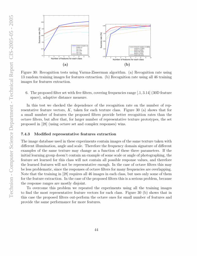
1 2 3 4 5 6 7 8 9 100.7

0.75

0.8

0.85

0.9

0.95

1

Number of features for each class

Suc

cess

rat

e (%

)

Octave Complex L2Octave L2Our 3 L2Our 3 AMOur 5 L2Our 5 AM

1 2 3 4 5 6 7 8 9 100.75

0.8

0.85

0.9

0.95

Number of features for each class

Suc

cess

rat

e (%

)

Octave3 complex L2 (38D)Octave3 L2 (20D)MHD3 L2 (20D)MHD3 AM (20D)MHD5 L2 (32D)MHD5 AM (32D)

(a) (b)

Figure 30: Recognition tests using Varma-Zisserman algorithm. (a) Recognition rate using13 random training images for features extraction. (b) Recognition rate using all 46 trainingimages for features extraction.

6. The proposed filter set with five filters, covering frequencies range [.1, 3.14] (30D featurespace), adaptive distance measure.

In this test we checked the dependence of the recognition rate on the number of rep-resentative feature vectors, K, taken for each texture class. Figure 30 (a) shows that fora small number of features the proposed filters provide better recognition rates than theoctave filters, but after that, for larger number of representative texture prototypes, the setproposed in [28] (using octave set and complex responses) wins.

7.4.3 Modified representative features extraction

The image database used in these experiments contain images of the same texture taken withdifferent illumination, angle and scale. Therefore the frequency domain signature of differentexamples of the same texture may change as a function of these three parameters. If theinitial learning group doesn’t contain an example of some scale or angle of photographing, thefeature set learned for this class will not contain all possible response values, and thereforethe learned features will not be representative enough. In the case of octave filters this maybe less problematic, since the responses of octave filters for many frequencies are overlapping.Note that the training in [28] requires all 46 images in each class, but uses only some of themfor the feature extraction. In the case of the proposed filters this is a serious problem, becausethe response ranges are mostly disjoint.

To overcome this problem we repeated the experiments using all the training imagesto find the most representative feature vectors for each class. Figure 30 (b) shows that inthis case the proposed filters out-perform the octave ones for small number of features andprovide the same performance for more features.

44

Tec

hnio

n -

Com

pute

r Sc

ienc

e D

epar

tmen

t - T

echn

ical

Rep

ort

CIS

-200

5-05

- 2

005

8 Conclusions

A novel method for constructing set of Gabor filters was proposed. Unlike the commonlyused filter sets which concentrate on the optimal representation (in MSE sense) of the sig-nals, the main consideration in constructing the proposed set is maximizing the number ofdistinguished signal pairs.

The method is based on analytical and semi-analytical derivations of the optimal filtersets for separating harmonic signals. It was also analytically shown that the proposed filtersare reasonable for signals with several harmonics. The proposed filter sets are extended to2D and a special, based on analytical properties of the filters, Mahalanobis-like distancemeasure was proposed to compare the resulting features.

It was shown in experiments with real-life texture samples that the proposed filters aresuperior than the commonly used ones in the task of image segmentation, even using suchprimitive methods as K-means. It was also shown that for a reasonable small set of textures,the proposed method provides a stable recognition of texture members, given representativeof each texture. Note, that the proposed filters performed better using a common L2 metricfor features comparing. Using a new adaptive distance measure improved the results for theproposed filters and didn’t change the results for the commonly used filters.

The difference in filter set building considerations caused that the obtained filter setsare significantly different from the commonly used ones. The representation based filter setsachieve better reconstruction of the texture from the response coefficients in each location onthe texture, but this may cause a very different responses in different locations. The responsedistribution comparing methods deal with this phenomenon, but they are computationallyhard. The responses of the proposed filters to textured signals are less varying with trans-lation than the responses to the commonly used filters. This allows to use a single featurevector to describe each texture. In context of segmentation of natural textured images thisis a simpler and faster method.

The proposed method fits the main goal of the work: the distance between featurevectors of pixels from the same texture is mostly smaller than the distance to pixels fromother textures. However, since the goal was to describe each texture by a single featurevector, this method may work worse than the distribution based ones for textures with largevariability of responses.

The next step in this work seems to be an integration of the proposed filter sets intocomplex segmentation algorithms, mentioned in the beginning of the work. Another directionmay be development of a new fast segmentation algorithm which would use the specialproperties of the proposed features, such as a good separation using a simple thresholdcriterion. Considering geometrical properties of compared pixels should increase even morethe high distinguishability power of the proposed features. The segmentation tasks usuallyimply that inter texture distances are small, therefore the stability of responses in the sametexture of the proposed features should increase the segmentation quality.

45

Tec

hnio

n -

Com

pute

r Sc

ienc

e D

epar

tmen

t - T

echn

ical

Rep

ort

CIS

-200

5-05

- 2

005

9 Acknowledgements

We would like to thank the creators of the CUReT database for enabling us to use it, andto Manik Varma, who let us use the processed version of their database as well. We wouldlike to thank Ilan Shimshoni for providing us an implementation of meanshift clusteringalgorithm. We thank Israeli science foundation for financial support of this research.

46

Tec

hnio

n -

Com

pute

r Sc

ienc

e D

epar

tmen

t - T

echn

ical

Rep

ort

CIS

-200

5-05

- 2

005

A A response to single harmonic signal

The absolute value of the Gabor filter hk,σ2(x) = 1√2πσ2

e−x2

2σ2 +ikx response to a signal gm,A(x),is

|hk,σ2(x) ∗ gm,A(x)| =

√

(Re(hk,σ2(x) ∗ gm,A(x)))2 + (Im(hk,σ2(x) ∗ gm,A(x)))2

For gm,A(x) = Asin(mx) the Real part response is:

Re(hk,σ2(x) ∗ gm,A(x)) =1√

2πσ2e

−x2

2σ2 sin(kx) ∗ Asin(mx)

=A√2πσ2

∫ ∞

−∞e

−ξ2

2σ2 sin(kξ)sin(m(x − ξ)) dξ

=A√2πσ2

∫ ∞

−∞e

−ξ2

2σ2 sin(kξ) {sin(mx)cos(mξ) − cos(mx)sin(mξ)} dξ

=Asin(mx)√

2πσ2

∫ ∞

−∞e

−ξ2

2σ2 sin(kξ)cos(mξ) dξ

−Acos(mx)√2πσ2

∫ ∞

−∞e

−ξ2

2σ2 sin(kξ)sin(mξ) dξ

=Asin(mx)√

8πσ2

∫ ∞

−∞e

−ξ2

2σ2 {sin((k + m)ξ) + sin((k − m)ξ)} dξ

−Acos(mx)√8πσ2

∫ ∞

−∞e

−ξ2

2σ2 {cos((k − m)ξ) − cos((k + m)ξ)} dξ

=Acos(mx)√

8πσ2

∫ ∞

−∞e

−ξ2

2σ2 {cos((k + m)ξ) − cos((k − m)ξ)} dξ

= ∗ A

2

{

e−(k+m)2σ2

2 − e−(k−m)2σ2

2

}

cos(mx)

=A

2e

−(k2+m2)σ2

2

{

e−kmσ2 − ekmσ2}

cos(mx)

= −Ae−(k2+m2)σ2

2 sh(kmσ2)cos(mx)

where * is due to∫∞0

e−a2x2cos(mx)dx =

√π

2ae−

m2

4a2

47

Tec

hnio

n -

Com

pute

r Sc

ienc

e D

epar

tmen

t - T

echn

ical

Rep

ort

CIS

-200

5-05

- 2

005

For gm,A(x) = Acos(mx) the Real part response is:

Re(hk,σ2(x) ∗ gm,A(x)) =1√

2πσ2e

−x2

2σ2 sin(kx) ∗ Acos(mx)

=A√2πσ2

∞

−∞e

−ξ2

2σ2 sin(kξ)sin(π

2− m(x − ξ)) dξ

=A√2πσ2

∞

−∞e

−ξ2

2σ2 sin(kξ){

sin(π

2)cos(m(x − ξ)) − cos(

π

2)sin(m(x − ξ))

}

dξ

=A√2πσ2

∞

−∞e

−ξ2

2σ2 sin(kξ) {cos(m(x − ξ))} dξ

=A√2πσ2

∞

−∞e

−ξ2

2σ2 sin(kξ) {cos(mx)cos(mξ) − sin(mx)sin(mξ)} dξ

=Acos(mx)√

2πσ2

∞

−∞e

−ξ2

2σ2 sin(kξ)cos(mξ) dξ

−Asin(mx)√2πσ2

∞

−∞e

−ξ2

2σ2 sin(kξ)sin(mξ) dξ

=Acos(mx)√

8πσ2

∞

−∞e

−ξ2

2σ2 {sin((k + m)ξ) + sin((k − m)ξ)} dξ

−Asin(mx)√8πσ2

∞

−∞e

−ξ2

2σ2 {cos((k − m)ξ) − cos((k + m)ξ)} dξ

=Asin(mx)√

8πσ2

∞

−∞e

−ξ2

2σ2 {cos((k + m)ξ) − cos((k − m)ξ)} dξ

= ∗ A

2

{

e−(k+m)2σ2

2 − e−(k−m)2σ2

2

}

sin(mx)

=A

2e

−(k2+m2)σ2

2

{

e−kmσ2 − ekmσ2}

sin(mx)

= −Ae−(k2+m2)σ2

2 sh(kmσ2)sin(mx)

where * is due to∫∞0

e−a2x2cos(mx)dx =

√π

2ae−

m2

4a2

48

Tec

hnio

n -

Com

pute

r Sc

ienc

e D

epar

tmen

t - T

echn

ical

Rep

ort

CIS

-200

5-05

- 2

005

For gm,A(x) = Asin(mx) the imaginary part response is:

Im(hk,σ2(x) ∗ gm,A(x)) =1√

2πσ2e

−x2

2σ2 cos(kx) ∗ Asin(mx)

=A√2πσ2

∫ ∞

−∞e

−ξ2

2σ2 cos(kξ)sin(m(x − ξ)) dξ

=A√2πσ2

∫ ∞

−∞e

−ξ2

2σ2 cos(kξ) {sin(mx)cos(mξ) − cos(mx)sin(mξ)} dξ

=Asin(mx)√

2πσ2

∫ ∞

−∞e

−ξ2

2σ2 cos(kξ)cos(mξ) dξ

−Acos(mx)√2πσ2

∫ ∞

−∞e

−ξ2

2σ2 cos(kξ)sin(mξ)) dξ

=Asin(mx)√

8πσ2

∫ ∞

−∞e

−ξ2

2σ2 {cos((k + m)ξ) + cos((k − m)ξ)} dξ

= −Acos(mx)√8πσ2

∫ ∞

−∞e

−ξ2

2σ2 {sin((k − m)ξ) + sin((k + m)ξ)}cos(mx) dξ

=Asin(mx)√

8πσ2

∫ ∞

−∞e

−ξ2

2σ2 {cos((k + m)ξ) + cos((k − m)ξ)} dξ

=A

2

{

e−(k−m)2σ2

2 + e−(k+m)2σ2

2

}

sin(mx)

=A

2e

−(k2+m2)σ2

2

{

ekmσ2

+ e−kmσ2}

sin(mx)

= Ae−(k2+m2)σ2

2 ch(kmσ2)sin(mx)

49

Tec

hnio

n -

Com

pute

r Sc

ienc

e D

epar

tmen

t - T

echn

ical

Rep

ort

CIS

-200

5-05

- 2

005

For gm,A(x) = Acos(mx) the imaginary part response is:

Im(hk,σ2(x) ∗ gm,A(x)) =1√

2πσ2e

−x2

2σ2 cos(kx) ∗ cos(mx)

=A√2πσ2

∫ ∞

−∞e

−ξ2

2σ2 cos(kξ)sin(π

2− m(x − ξ)) dξ

=A√2πσ2

∫ ∞

−∞e

−ξ2

2σ2 cos(kξ){

sin(π

2)cos(m(x − ξ)) − cos(

π

2)sin(m(x − ξ))

}

dξ

=A√2πσ2

∫ ∞

−∞e

−ξ2

2σ2 cos(kξ) {cos(mx)cos(mξ) − sin(mx)sin(mξ)} dξ

=Acos(mx)√

2πσ2

∫ ∞

−∞e

−ξ2

2σ2 cos(kξ)cos(mξ) dξ

−Asin(mx)√2πσ2

∫ ∞

−∞e

−ξ2

2σ2 cos(kξ)sin(mξ) dξ

=Acos(mx)√

8πσ2

∫ ∞

−∞e

−ξ2

2σ2 {cos((k + m)ξ) + cos((k − m)ξ)} dξ

−Asin(mx)√8πσ2

∫ ∞

−∞e

−ξ2

2σ2 {sin((k − m)ξ) + sin((k + m)ξ)} dξ

=Acos(mx)√

8πσ2

∫ ∞

−∞e

−ξ2

2σ2 {cos((k + m)ξ) + cos((k − m)ξ)} dξ

=A

2

{

e−(k−m)2σ2

2 + e−(k+m)2σ2

2

}

cos(mx)

=A

2e

−(k2+m2)σ2

2

{

ekmσ2

+ e−kmσ2}

cos(mx)

= Ae−(k2+m2)σ2

2 ch(kmσ2)cos(mx)

Thus, for gm,A(x) = Asin(mx) the absolute value of the response is:

|hk,σ2(x) ∗ gm,A(x)| = A√

e−(k2+m2)σ2sh2(kmσ2)cos2(mx) + e−(k2+m2)σ2ch2(kmσ2)sin2(mx)

= Ae−(k2+m2)σ2

2

√

sh2(kmσ2)cos2(mx) + ch2(kmσ2)sin2(mx)

= Ae−(k2+m2)σ2

2

√

1

2(ch(2kmσ2) − 1)cos2(mx) +

1

2(ch(2kmσ2) + 1)sin2(mx)

= Ae−(k2+m2)σ2

2

√

1

2ch(2kmσ2){cos2(mx) + sin2(mx)} +

1

2{sin2(mx) − cos2(mx)}

= Ae−(k2+m2)σ2

2

√

1

2ch(2kmσ2) − 1

2cos(2mx)

= Ae−(k2+m2)σ2

2

√

ch2(kmσ2) − cos2(mx)

50

Tec

hnio

n -

Com

pute

r Sc

ienc

e D

epar

tmen

t - T

echn

ical

Rep

ort

CIS

-200

5-05

- 2

005

and for gm,A(x) = Acos(mx) the absolute value of the response is:

|hk,σ2(x) ∗ gm,A(x)| = A√

e−(k2+m2)σ2sh2(kmσ2)sin2(mx) + e−(k2+m2)σ2ch2(kmσ2)cos2(mx)

= Ae−(k2+m2)σ2

2

√

sh2(kmσ2)sin2(mx) + ch2(kmσ2)cos2(mx)

= Ae−(k2+m2)σ2

2

√

1

2(ch(2kmσ2) − 1)sin2(mx) +

1

2(ch(2kmσ2) + 1)cos2(mx)

= Ae−(k2+m2)σ2

2

√

1

2ch(2kmσ2){cos2(mx) + sin2(mx)} +

1

2{cos2(mx) − sin2(mx)}

= Ae−(k2+m2)σ2

2

√

1

2ch(2kmσ2) +

1

2cos(2mx)

= Ae−(k2+m2)σ2

2

√

ch2(kmσ2) − sin2(mx)

B A response to dual-harmonic signal

The absolute value of the Gabor filter hk,σ2(x) = 1√2πσ2

e−x2

2σ2 +ikx response to a dual harmonic

signal g~m, ~A

(x) = Asin(m1x) + Bsin(m2x), is

|hk,σ2(x) ∗ g~m, ~A

(x)| = |hk,σ2(x) ∗ Asin(m1x) + hk,σ2(x) ∗ Bsin(m2x)|

=

{

(

Ae−(k2+m2

1)σ2

2 sh(km1σ2)cos(m1x) + Be−

(k2+m22)σ2

2 sh(km2σ2)cos(m2x)

)2

+

(

Ae−(k2+m2

1)σ2

2 ch(km1σ2)sin(m1x) + Be−

(k2+m22)σ2

2 ch(km2σ2)sin(m2x)

)2}

12

=

{(

(

Ae−(k2+m2

1)σ2

2 sh(km1σ2)cos(m1x)

)2

+

(

Ae−(k2+m2

1)σ2

2 ch(km1σ2)sin(m1x)

)2)

+

(

(

Be−(k2+m2

2)σ2

2 sh(km2σ2)cos(m2x)

)2

+

(

Be−(k2+m2

2)σ2

2 ch(km2σ2)sin(m2x)

)2)

+2Ae−(k2+m2

1)σ2

2 sh(km1σ2)cos(m1x)Be−

(k2+m22)σ2

2 sh(km2σ2)cos(m2x)

+2Ae−(k2+m2

1)σ2

2 ch(km1σ2)sin(m1x)Be−

(k2+m22)σ2

2 ch(km2σ2)sin(m2x)

}12

={

A2e−(k2+m21)σ2 (

ch2(km1σ2) − cos2(m1x)

)

+ B2e−(k2+m22)σ2 (

ch2(km2σ2) − cos2(m2x)

)

+2Ae−(k2+m2

1)σ2

2 Be−(k2+m2

2)σ2

2 ·(

sh(km1σ2)cos(m1x)sh(km2σ

2)cos(m2x) + ch(km1σ2)sin(m1x)ch(km2σ

2)sin(m2x))}

12

51

Tec

hnio

n -

Com

pute

r Sc

ienc

e D

epar

tmen

t - T

echn

ical

Rep

ort

CIS

-200

5-05

- 2

005

since ch(x) > 0 for all x-s,we can bound the received result with:

max{|h ∗ g|} ={

A2e−(k2+m21)σ2

ch2(km1σ2) + B2e−(k2+m2

2)σ2

ch2(km2σ2)

+Ae−(k2+m2

1)σ2

2 Be−(k2+m2

2)σ2

2

[

ch(kσ2(m1 + m2)) + ch(kσ2(m1 − m2))]

}12

={

A2e−(k2+m21)σ2

ch2(km1σ2) + B2e−(k2+m2

2)σ2

ch2(km2σ2)

+2Ae−(k2+m2

1)σ2

2 Be−(k2+m2

2)σ2

2 ch(km1σ2)ch(km2σ

2)

}12

= Ae−(k2+m2

1)σ2

2 ch(km1σ2) + Be−

(k2+m22)σ2

2 ch(km2σ2)

min{|h ∗ g|} ={

A2e−(k2+m21)σ2

sh2(km1σ2) + B2e−(k2+m2

2)σ2

sh2(km2σ2)

−2Ae−(k2+m2

1)σ2

2 Be−(k2+m2

2)σ2

2

[

sh(km1σ2)sh(km2σ

2)]

}12

=

∣

∣

∣

∣

Ae−(k2+m2

1)σ2

2 sh2(km1σ2) − Be−

(k2+m22)σ2

2 sh2(km2σ2)

∣

∣

∣

∣

The absolute value of the Gabor filter hk,σ2(x) = 1√2πσ2

e−x2

2σ2 +ikx response to a dual har-

52

Tec

hnio

n -

Com

pute

r Sc

ienc

e D

epar

tmen

t - T

echn

ical

Rep

ort

CIS

-200

5-05

- 2

005

monic signal g~m, ~A(x) = Asin(m1x) + Bcos(m2x), is

|hk,σ2(x) ∗ g~m, ~A(x)| = |hk,σ2(x) ∗ Asin(m1x) + hk,σ2(x) ∗ Bcos(m2x)|

=

{

(

Ae−(k2+m2

1)σ2

2 sh(km1σ2)cos(m1x) + Be−

(k2+m22)σ2

2 sh(km2σ2)sin(m2x)

)2

+

(

Ae−(k2+m2

1)σ2

2 ch(km1σ2)sin(m1x) + Be−

(k2+m22)σ2

2 ch(km2σ2)cos(m2x)

)2}

12

=

{(

(

Ae−(k2+m2

1)σ2

2 sh(km1σ2)cos(m1x)

)2

+

(

Ae−(k2+m2

1)σ2

2 ch(km1σ2)sin(m1x)

)2)

+

(

(

Be−(k2+m2

2)σ2

2 sh(km2σ2)sin(m2x)

)2

+

(

Be−(k2+m2

2)σ2

2 ch(km2σ2)cos(m2x)

)2)

+2Ae−(k2+m2

1)σ2

2 sh(km1σ2)cos(m1x)Be−

(k2+m22)σ2

2 sh(km2σ2)sin(m2x)

+2Ae−(k2+m2

1)σ2

2 ch(km1σ2)sin(m1x)Be−

(k2+m22)σ2

2 ch(km2σ2)cos(m2x)

}12

={

A2e−(k2+m21)σ2 (

ch2(km1σ2) − cos2(m1x)

)

+ B2e−(k2+m22)σ2 (

ch2(km2σ2) − sin2(m2x)

)

+2Ae−(k2+m2

1)σ2

2 Be−(k2+m2

2)σ2

2 ·(

sh(km1σ2)cos(m1x)sh(km2σ

2)sin(m2x) + ch(km1σ2)sin(m1x)ch(km2σ

2)cos(m2x))}

12

since ch(x) > 0 for all x-s,we can bound the received result with:

max{|h ∗ g|} ={

A2e−(k2+m21)σ2

ch2(km1σ2) + B2e−(k2+m2

2)σ2

ch2(km2σ2)

+2Ae−(k2+m2

1)σ2

2 Be−(k2+m2

2)σ2

2 ch(km1σ2)ch(km2σ

2)

}12

= Ae−(k2+m2

1)σ2

2 ch(km1σ2) + Be−

(k2+m22)σ2

2 ch(km2σ2)

min{|h ∗ g|} ={

A2e−(k2+m21)σ2

sh2(km1σ2) + B2e−(k2+m2

2)σ2

sh2(km2σ2)

−2Ae−(k2+m2

1)σ2

2 Be−(k2+m2

2)σ2

2

[

sh(km1σ2)sh(km2σ

2)]

}12

=

∣

∣

∣

∣

Ae−(k2+m2

1)σ2

2 sh2(km1σ2) − Be−

(k2+m22)σ2

2 sh2(km2σ2)

∣

∣

∣

∣

53

Tec

hnio

n -

Com

pute

r Sc

ienc

e D

epar

tmen

t - T

echn

ical

Rep

ort

CIS

-200

5-05

- 2

005

C A response to multi-harmonic signal

In analogy to the bounds on the response of a single sine signal to a filter, described inprevious appendix, we have developed an expression for a filter response to a signal whichis a sum of sines with different amplitudes.

Consider a complex Gabor filter hk(x) = 1√2πσ2

e−x2

2σ2 +ikx, and a signal g ~A,~m(x) =∑

i Aisin(mix).It can be shown that the filter response:

r ~A,k,~m(x) = hk(x) ∗ gA,m(x) (C.1)

=

{

∑

i

A2i e

−(k2+m2i )σ2 [

ch2(kmiσ2) − cos2(mix)

]

+∑

i,j;i6=j

Aie− (k2+m2

i )σ2

2 Aje−

(k2+m2j )σ2

2 ·

·(

ch[kσ2(mi + mj)]cos[(mi − mj)x]

− ch[kσ2(mi − mj)]cos[(mi + mj)x]

)

}12

The upper bound of this expression is:

max

{∣

∣

∣

∣

∣

hk(x) ∗∑

i

Aisin(mix)

∣

∣

∣

∣

∣

}

=∑

i

Aie− (k2+m2

i )σ2

2 ch(kmiσ2)

A lower bound depends in a complex way on the combination of mi frequencies andamplitudes Ai. We could not find a useful lower bound and just use the trivial one, whichis zero.

Thus,N∑

i=1

Aie−(k2+m2

i )σ2

2 ch(kmiσ2) ≥ r ~A,~m,k,σ2(x) ≥ 0 (C.2)

Relating on the upper bound as the actual maximal response and use the trivial lower boundimplies that

r ~A1,k,~m,σ2 ≥ 12

{

∑N

i=1 Aie−(k2+m2

i )σ2

2 ch(kmiσ2)

}

∆r ~A,k,~m,σ2 ≤∑N

i=1 Aie−(k2+m2

i )σ2

2 ch(kmiσ2) (C.3)

Applying ∆m estimation to this approximation:

∆m ∼=∆r ~A,~m,k,σ2∣

∣

∣∇r ~A,k,~m,σ2

∣

∣

∣

≤∑N

i=1 Aie−(k2+m2

i )σ2

2 ch(kmiσ2)

∑N

i=1 Aie−(k2+m2

i)σ2

2 |k · sh(kmiσ2) − m1 · ch(kmiσ2)|σ2

54

Tec

hnio

n -

Com

pute

r Sc

ienc

e D

epar

tmen

t - T

echn

ical

Rep

ort

CIS

-200

5-05

- 2

005

Note, that this time the middle response is multidimensional function. To obtain a linearapproximation for its change tempo we should consider the direction of maximal change,i.e. the gradient. Note also, that the received expression is an upper bound on ∆m. Thedividend may be only smaller. The divisor an absolute value of a gradient of some Gaussian-like function, which tails are always near zero, but the maximal value may only increase.The absolute value of the gradient of such function may only increase. Therefore the totalfraction is bounded from above by the given expression.

For large σ (sh(kmiσ2) ≃ sh(kmiσ

2)) ≃ 12ekmiσ

2), it may be simplified to

∆m ≤∑N

i=1 Aie−(k−mi)

2σ2

2

∑N

i=1 Aie−(k−mi)

2σ2

2 |k − mi|σ2. (C.4)

The obtained expression gets its maximum at k = mi similarly to the two frequenciescase (4.29). Thus, the filters design considerations for dual-harmonic signals are identical tothose of the multi-harmonic case.

D Optimality of the chosen single filter

If a response in fmin have to be equal Rmin, the σ2 of the filter is given by:

σ2 =−2log(Rmin)

(k − fmin)2(D.1)

If we increase k by δ the new σ2 would be:

σ2δ =

−2log(Rmin)

(k + δ − fmin)2(D.2)

The ∆m measure for fmin and filter k, σ is given by:

∆mǫ =e−2kfminσ2

(k − fmin)σ2=

e−−4log(Rmin)kfmin

2(k−fmin)2

(k − fmin)−2log(Rmin)(k−fmin)2

(D.3)

=fmin − k

Ce

C[(k+fmin)2−(k−fmin)2]

2(k−fmin)2 (D.4)

=fmin − k

Ce

C

�(k+fmin)2

2(k−fmin)2− 1

2

�(D.5)

The ∆m measure for fmin and filter k + δ, σδis given by:

∆mǫδ= e−

(k+δ+fmin)2σ2δ

2 =fmin − k − δ

Ce

C

�(k+δ+fmin)2

2(k+δ−fmin)2− 1

2

�(D.6)

Since Rmin is a small number, its log is a negative number. Therefore C is a negativeconstant. Both k + fmin and k − fmin are above zero, therefore

(k + δ + fmin)2

(k + δ − fmin)2<

(k + fmin)2

(k − fmin)2(D.7)

and thus ∆mǫδ< ∆mǫ because its exponent value is less negative and its non-exponent factor

is smaller. Therefore increasing of the filter’s frequency and preserving the given responseat fmin would increase ∆m in filter’s responses.

55

Tec

hnio

n -

Com

pute

r Sc

ienc

e D

epar

tmen

t - T

echn

ical

Rep

ort

CIS

-200

5-05

- 2

005

E Ratio theorem

Theorem 1.1.{

rA1,m1,k1,σ21(x)

rA1,m1,k2,σ22(x)

, x ∈ R

}

⋂

{

rA2,m2,k1,σ21(x)

rA2,m2,k2,σ22(x)

, x ∈ R

}

= ∅

⇓{rA1,k1,m1,σ2

1(x), x ∈ R} ⋂ {rA2,k1,m2,σ2

1(x), x ∈ R} = ∅

or

{rA1,k2,m1,σ22(x), x ∈ R} ⋂ {rA2,k2,m2,σ2

2(x), x ∈ R} = ∅

Proof: Suppose the claim is wrong, then w.l.g.

{

rA1,m1,k1,σ21(x)

rA1,m1,k2,σ22(x)

, x ∈ R

}

⋂

{

rA2,m2,k1,σ21(x)

rA2,m2,k2,σ22(x)

, x ∈ R

}

= ∅

and

{rA1,k1,m1,σ21(x), x ∈ R} ⋂ {rA2,k1,m2,σ2

1(x), x ∈ R} 6= ∅

and

{rA1,k2,m1,σ22(x), x ∈ R} ⋂ {rA2,k2,m2,σ2

2(x), x ∈ R} 6= ∅

which is:

min{rA1,m1,k1,σ21(x)}

max{rA1,m1,k2,σ22(x)} >

max{rA2,m2,k1,σ21(x)}

min{rA2,m2,k2,σ22(x)}

and

min{rA1,m1,k1,σ21(x)} < max{rA2,m2,k1,σ2

1(x)}

and

min{rA2,m2,k2,σ22(x)} < max{rA1,m1,k2,σ2

2(x)}

combining the latter two expressions:

min{rA1,m1,k1,σ21(x)}

max{rA1,m1,k2,σ22(x)} >

max{rA2,m2,k1,σ21(x)}

min{rA2,m2,k2,σ22(x)}

andmax{rA2,m2,k1,σ2

1(x)}

min{rA2,m2,k2,σ22(x)} > 1 >

min{rA1,m1,k1,σ21(x)}

max{rA1,m1,k2,σ22(x)}

we reached a contradiction, therefore the assumption was wrong, w.s.p.

56

Tec

hnio

n -

Com

pute

r Sc

ienc

e D

epar

tmen

t - T

echn

ical

Rep

ort

CIS

-200

5-05

- 2

005

References

[1] B.B.Mandelbrot, The fractal geometry of nature, New York: W.H. Freeman, 1983.

[2] K. Brady, I.H. Jermyn, and J.Zerubia, Adaptive probabilistic models of wavelet packetsfor the analysis and segmentation of textured remote sensing images, Proceedings of theBritish Machine Vision Conference (2003).

[3] R. Chellappa and S. Chatterjee, Classification of textures using gaussian markov randomfield, IEEE Transactions on Acoustics, Speech and Signal Processing 33 (1985), no. 4,959–963.

[4] G.R. Cross and A.K. Jain, Markov random field texture models, TransPAMI 5 (1983),25–39.

[5] K.J. Dana, B. van Ginneken, S.K. Nayar, and J. J. Koenderink, Reflectance and textureof real world surfaces, ACM Transactions on Graphics 18 (1999), no. 1, 1–34.

[6] J.G. Daugman, Uncertainty relation for resolution , spatial frequency, and orientationoptimized by 2d visual cortical filters, Journal of the Optical Society of America A 2(1985), 1160–1169.

[7] D.J.Field, Relation between the statistics of natural images and the response propertiesof cortical cell, J.Opt.Soc.Am.A 4 (1987), no. 12, 2379–2394.

[8] I. Fogel and D. Sagi, Gabor filters as texture discriminator, BioCyber 61 (1989), 102–113.

[9] D. Gabor, Theory of communication, J.IEE 93 (1946), 429–459.

[10] B. Georgescu, I. Shimshoni, and P. Meer, Mean shift based clustering in high dimensions:A texture classification example., 9th International Conference on Computer Vision(2003), 456–463.

[11] H. Greenspan, Multi-resolution image processing and learning for texture recog-nition and image enhancement, Ph.d. thesis, California Institute of Technology,Pasadena,California, May 1994.

[12] H. Greenspan, S. Belongie, P. Perona, R. Goodman, S. Rackshit, and C.H.Anderson,Overcomplete steerable pyramid filters and rotation invariance, Proc. of the IEEE Con-ference on Computer Vision and Pattern Recognition (1994).

[13] R.M. Haralick, K. Shanmugam, and I. Dinstein, Textural features for image classifica-tion, SMC (1973), 611–621.

[14] J.M. Jolion, Feature similarity (in principles of visual information retrieval), ch. I.5,Springer, 2000.

[15] K.I.Laws, Textured image segmentation, Ph.D. thesis, Dept. Electrical Engineer-ing,University of Southern California, January 1980.

57

Tec

hnio

n -

Com

pute

r Sc

ienc

e D

epar

tmen

t - T

echn

ical

Rep

ort

CIS

-200

5-05

- 2

005

[16] T. S. Lee, Image representation using 2d gabor wavelets, IEEE Transactions on PatternAnalysis and Machine Intelligence 18 (1996), no. 10, 959–971.

[17] T. Leung and J. Malik, Representing and recognizing the visual appearance of materialsusing three-dimensional textons, International Journal of Computer Vision 43 (2001),no. 1, 29–44.

[18] W.Y. Ma and B.S. Manjunath, Edgeflow: A technique for boundary detection and imagesegmentation.

[19] J. Malik, S. Belongie, T. K. Leung, and J. Shi, Contour and texture analysis for imagesegmentation, International Journal of Computer Vision 43 (2001), no. 1, 7–27.

[20] J. Malik and P. Perona, Preattentive texture discrimination with early vision mechanism,JOSA-A 7 (1990), no. 5, 923–932.

[21] J. Mao and A.K. Jain, Texture classification and segmentation using multiresolutionsimultaneous autoregressive models, Pattern recognition 25 (1992), no. 2, 173–188.

[22] M.Porat and Y.Y.Zeevi, Localized texture processing in vision: Analysis and synthesisin the gaborian space, IEEE Trans Biomed Eng (1989), 115–29.

[23] A.P. Pentland, Fractal-based description of natural scenes, PAMI 6 (1984), no. 6, 661–674.

[24] Y. Rubner, Perceptual metrics for image database navigation, Ph.D. thesis, StanfordUniversity, 1999.

[25] E. Sharon, A. Brandt, and R. Basri, Fast multiscale image segmentation, IEEE Inter-national Conference in Computer Vision (1999), 70–77.

[26] J. Shi and J. Malik Self inducing relational distance and its application to image seg-mentation, EVVC (1), 1998, pp. 528–543.

[27] T.Randen and J.H.Husoy, Filtering for texture classification: A comparative study,PAMI 21 (1999), no. 4, 291–310.

[28] M. Varma and A. Zisserman, Classifying images of materials: Achieving viewpoint andillumination independence, Proceedings of the 7th European Conference on ComputerVision, Copenhagen, Denmark, vol. 3, May 2002, pp. 255–271.

[29] M. Varma and A. Zisserman, Texture classification: Are filter banks necessary?, Pro-ceedings of the IEEE Conference on Computer Vision and Pattern Recognition, vol. 2,June 2003, pp. 691–698.

[30] T. P. Weldon, W. E. Higgins, and D. F. Dunn, Efficient Gabor filter design for texturesegmentation, Pattern Recognition 29 (1996), no. 12, 2005–2015.

58

Tec

hnio

n -

Com

pute

r Sc

ienc

e D

epar

tmen

t - T

echn

ical

Rep

ort

CIS

-200

5-05

- 2

005