Embed Size (px)
Citation preview

G. Cowan Statistics for HEP / LAL Orsay, 3-5 January 2012 / Lecture 3 1
Statistical Methods for Particle PhysicsLecture 3: More on discovery and limits
Cours d’hiver 2012 du LALOrsay, 3-5 January, 2012
Glen CowanPhysics DepartmentRoyal Holloway, University of [email protected]/~cowan
http://www.pp.rhul.ac.uk/~cowan/stat_orsay.html

G. Cowan Statistics for HEP / LAL Orsay, 3-5 January 2012 / Lecture 3 2
Outline
Lecture 1: Introduction and basic formalism Probability, statistical tests, confidence intervals.
Lecture 2: Tests based on likelihood ratios Systematic uncertainties (nuisance parameters)
Limits for Poisson mean
Lecture 3: More on discovery and limits Upper vs. unified limits (F-C) Spurious exclusion, CLs, PCL Look-elsewhere effect Why 5σ for discovery?

G. Cowan Statistics for HEP / LAL Orsay, 3-5 January 2012 / Lecture 3 3
Reminder about statistical tests
Consider test of a parameter μ, e.g., proportional to cross section.
Result of measurement is a set of numbers x.
To define test of μ, specify critical region wμ, such that probabilityto find x ∈ wμ is not greater than α (the size or significance level):
(Must use inequality since x may be discrete, so there may not exist a subset of the data space with probability of exactly α.)
Equivalently define a p-value pμ such that the critical region corresponds to pμ < α.
Often use, e.g., α = 0.05.
If observe x ∈ wμ, reject μ.

G. Cowan Statistics for HEP / LAL Orsay, 3-5 January 2012 / Lecture 3 4
Confidence interval from inversion of a test
Carry out a test of size α for all values of μ.
The values that are not rejected constitute a confidence intervalfor μ at confidence level CL = 1 – α.
The confidence interval will by construction contain thetrue value of μ with probability of at least 1 – α.
The interval depends on the choice of the test, which is often based on considerations of power.

G. Cowan Statistics for HEP / LAL Orsay, 3-5 January 2012 / Lecture 3 5
Power of a statistical test
Where to define critical region? Usually put this where thetest has a high power with respect to an alternative hypothesis μ′.
The power of the test of μ with respect to the alternative μ′ isthe probability to reject μ if μ′ is true:
(M = Mächtigkeit,мощность)
p-value of hypothesized μ

G. Cowan Statistics for HEP / LAL Orsay, 3-5 January 2012 / Lecture 3 6
Choice of test for limitsSuppose we want to ask what values of μ can be excluded on the grounds that the implied rate is too high relative to what isobserved in the data.
The interesting alternative in this context is μ = 0.
The critical region giving the highest power for the test of μ relativeto the alternative of μ = 0 thus contains low values of the data.
Test based on likelihood-ratio with respect toone-sided alternative → upper limit.

I.e. for purposes of setting an upper limit, one does not regardan upwards fluctuation of the data as representing incompatibilitywith the hypothesized μ.
From observed qμ find p-value:
Large sample approximation:
95% CL upper limit on μ is highest value for which p-value is not less than 0.05.
G. Cowan Statistics for HEP / LAL Orsay, 3-5 January 2012 / Lecture 3 7
Test statistic for upper limitsFor purposes of setting an upper limit on μ use
where

G. Cowan Statistics for HEP / LAL Orsay, 3-5 January 2012 / Lecture 3 8
Choice of test for limits (2)In other cases we want to exclude μ on the grounds that some othermeasure of incompatibility between it and the data exceeds somethreshold.
For example, the process may be known to exist, and thus μ = 0is no longer an interesting alternative.
If the measure of incompatibility is taken to be the likelihood ratiowith respect to a two-sided alternative, then the critical region can contain both high and low data values. → unified intervals, G. Feldman, R. Cousins,
Phys. Rev. D 57, 3873–3889 (1998)
The Big Debate is whether to use one-sided or unified intervalsin cases where the relevant alternative is at small (or zero) valuesof the parameter. Professional statisticians have voiced supporton both sides of the debate.

9
Unified (Feldman-Cousins) intervals
We can use directly
G. Cowan Statistics for HEP / LAL Orsay, 3-5 January 2012 / Lecture 3
as a test statistic for a hypothesized μ.
where
Large discrepancy between data and hypothesis can correspondeither to the estimate for μ being observed high or low relativeto μ.
This is essentially the statistic used for Feldman-Cousins intervals(here also treats nuisance parameters). G. Feldman and R.D. Cousins, Phys. Rev. D 57 (1998) 3873.
Lower edge of interval can be at μ = 0, depending on data.

10
Distribution of tμUsing Wald approximation, f (tμ|μ′) is noncentral chi-squarefor one degree of freedom:
G. Cowan Statistics for HEP / LAL Orsay, 3-5 January 2012 / Lecture 3
Special case of μ = μ′ is chi-square for one d.o.f. (Wilks).
The p-value for an observed value of tμ is
and the corresponding significance is

Statistics for HEP / LAL Orsay, 3-5 January 2012 / Lecture 3 11
Upper/lower edges of F-C interval for μ versus bfor n ~ Poisson(μ+b)
Lower edge may be at zero, depending on data.
For n = 0, upper edge has (weak) dependence on b.
Feldman & Cousins, PRD 57 (1998) 3873
G. Cowan

G. Cowan Statistics for HEP / LAL Orsay, 3-5 January 2012 / Lecture 3 12
Feldman-Cousins discussion
The initial motivation for Feldman-Cousins (unified) confidenceintervals was to eliminate null intervals.
The F-C limits are based on a likelihood ratio for a test of μ with respect to the alternative consisting of all other allowed valuesof μ (not just, say, lower values).
The interval’s upper edge is higher than the limit from the one-sided test, and lower values of μ may be excluded as well. A substantial downward fluctuation in the data gives a low (but nonzero) limit.
This means that when a value of μ is excluded, it is becausethere is a probability α for the data to fluctuate either high or lowin a manner corresponding to less compatibility as measured bythe likelihood ratio.

G. Cowan Statistics for HEP / LAL Orsay, 3-5 January 2012 / Lecture 3 13
Low sensitivity to μIt can be that the effect of a given hypothesized μ is very smallrelative to the background-only (μ = 0) prediction.
This means that the distributions f(qμ|μ) and f(qμ|0) will bealmost the same:

G. Cowan Statistics for HEP / LAL Orsay, 3-5 January 2012 / Lecture 3 14
Having sufficient sensitivity
In contrast, having sensitivity to μ means that the distributionsf(qμ|μ) and f(qμ|0) are more separated:
That is, the power (probability to reject μ if μ = 0) is substantially higher than α. Use this power as a measure of the sensitivity.

G. Cowan Statistics for HEP / LAL Orsay, 3-5 January 2012 / Lecture 3 15
Spurious exclusion
Consider again the case of low sensitivity. By construction the probability to reject μ if μ is true is α (e.g., 5%).
And the probability to reject μ if μ = 0 (the power) is only slightly greater than α.
This means that with probability of around α = 5% (slightly higher), one excludes hypotheses to which one has essentially no sensitivity (e.g., mH = 1000 TeV).
“Spurious exclusion”

G. Cowan Statistics for HEP / LAL Orsay, 3-5 January 2012 / Lecture 3 16
Ways of addressing spurious exclusion
The problem of excluding parameter values to which one hasno sensitivity known for a long time; see e.g.,
In the 1990s this was re-examined for the LEP Higgs search byAlex Read and others
and led to the “CLs” procedure for upper limits.
Unified intervals also effectively reduce spurious exclusion bythe particular choice of critical region.

G. Cowan Statistics for HEP / LAL Orsay, 3-5 January 2012 / Lecture 3 17
The CLs procedure
f (Q|b)
f (Q| s+b)
ps+bpb
In the usual formulation of CLs, one tests both the μ = 0 (b) andμ = 1 (s+b) hypotheses with the same statistic Q = 2ln Ls+b/Lb:

G. Cowan Statistics for HEP / LAL Orsay, 3-5 January 2012 / Lecture 3 18
The CLs procedure (2)
As before, “low sensitivity” means the distributions of Q under b and s+b are very close:
f (Q|b) f (Q|s+b)
ps+bpb

G. Cowan Statistics for HEP / LAL Orsay, 3-5 January 2012 / Lecture 3 19
The CLs solution (A. Read et al.) is to base the test not onthe usual p-value (CLs+b), but rather to divide this by CLb (~ one minus the p-value of the b-only hypothesis), i.e.,
Define:
Reject s+b hypothesis if: Reduces “effective” p-value when the two
distributions become close (prevents exclusion if sensitivity is low).
f (q|b) f (q|s+b)
CLs+b = ps+b
1CLb
= pb
The CLs procedure (3)

G. Cowan Statistics for HEP / LAL Orsay, 3-5 January 2012 / Lecture 3 20
Power Constrained Limits (PCL)CLs has been criticized because the exclusion is based on a ratioof p-values, which did not appear to have a solid foundation.
The coverage probability of the CLs upper limit is greater than the nominal CL = 1 α by an amount that is generally not reported.
Therefore we have proposed an alternative method for protectingagainst exclusion with little/no sensitivity, by regarding a value ofμ to be excluded if:
Here the measure of sensitivity is the power of the test of μwith respect to the alternative μ = 0:
Cowan, Cranmer, Gross, Vitells, arXiv:1105.3166

G. Cowan Statistics for HEP / LAL Orsay, 3-5 January 2012 / Lecture 3 21
Constructing PCL
First compute the distribution under assumption of the background-only (μ = 0) hypothesis of the “usual” upper limit μup with no power constraint.
The power of a test of μ with respect to μ = 0 is the fraction oftimes that μ is excluded (μup < μ):
Find the smallest value of μ (μmin), such that the power is atleast equal to the threshold Mmin.
The Power-Constrained Limit is:
G. Cowan Statistics for HEP / LAL Orsay, 3-5 January 2012 / Lecture 3 22
Upper limit on μ for x ~ Gauss(μ,σ) with μ ≥ 0
x

G. Cowan Statistics for HEP / LAL Orsay, 3-5 January 2012 / Lecture 3 23
Choice of minimum power
Choice of Mmin is convention. Formally it should be large relativeto α (5%). Earlier we have proposed
because in Gaussian example this means that one applies thepower constraint if the observed limit fluctuates down by one standard deviation.
For the Gaussian example, this gives μmin = 0.64σ, i.e., the lowest limit is similar to the intrinsic resolution of the measurement (σ).
More recently for several reasons we have proposed Mmin = 0.5, (which gives μmin = 1.64σ), i.e., one imposes the power constraint if the unconstrained limit fluctuations below its median under the background-only hypothesis.

G. Cowan Statistics for HEP / LAL Orsay, 3-5 January 2012 / Lecture 3 24
Comparison of reasons for (non)-exclusionSuppose we observe x = 1.
μ = 1 excluded by diag. line,why not by other methods?
PCL (Mmin=0.5): Because the power of a test of μ = 1 was below threshold.
CLs: Because the lack ofsensitivity to μ = 1 led toreduced 1 – pb, hence CLs not less than α.
F-C: Because μ = 1 was notrejected in a test of size α(hence coverage correct).But the critical region corresponding to more than half of α is at high x.
x

G. Cowan Statistics for HEP / LAL Orsay, 3-5 January 2012 / Lecture 3 25
Coverage probability for Gaussian problem

G. Cowan Statistics for HEP / LAL Orsay, 3-5 January 2012 / Lecture 3 26
More thoughts on power**thanks to Ofer Vitells
Synthese 36 (1):5 - 13.
Birnbaum formulates a concept of statistical evidencein which he states:

G. Cowan Statistics for HEP / LAL Orsay, 3-5 January 2012 / Lecture 3 27
More thoughts on power (2)**thanks to Ofer Vitells
This ratio is closely related to the exclusion criterion for CLs.
Birnbaum arrives at the conclusion above from the likelihood principle, which must be related to why CLs for the Gaussianand Poisson problems agree with the Bayesian result.

G. Cowan Statistics for HEP / LAL Orsay, 3-5 January 2012 / Lecture 3 28
Negatively Biased Relevant SubsetsConsider again x ~ Gauss(μ, σ) and use this to find limit for μ.
We can find the conditional probability for the limit to cover μ given x in some restricted range, e.g., x < c for some constant c.
This conditional coverage probability may be greater or less than 1 – α for different values of μ (the value of which is unkown).
But suppose that the conditional coverage is less than 1 – α for all values of μ. The region of x where this is true is a Negatively Biased Relevant Subset.
Recent studies by Bob Cousins (CMS) andOfer Vitells (ATLAS) related to earlier publications,especially, R. Buehler, Ann. Math. Sci., 30 (4) (1959) 845.See R. D. Cousins, arXiv:1109.2023

G. Cowan Statistics for HEP / LAL Orsay, 3-5 January 2012 / Lecture 3 29
Betting GamesSo what’s wrong if the limit procedure has NBRS?
Suppose you observe x, construct the confidence interval and assert that an interval thus constructed covers the true value of the parameter with probability 1 – α .
This means you should be willing to accept a bet at odds α : 1 – α that the interval covers the true parameter value.
Suppose your opponent accepts the bet if x is in the NBRS, and declines the bet otherwise. On average, you lose, regardless ofthe true (and unknown) value of μ.
With the “naive” unconstrained limit, if your opponent only accepts the bet when x < –1.64σ, (all values of μ excluded) you always lose!
(Recall the unconstrained limit based on the likelihood ratio never excludes μ = 0, so if that value is true, you do not lose.)

G. Cowan Statistics for HEP / LAL Orsay, 3-5 January 2012 / Lecture 3 30
NBRS for unconstrained upper limit
Maximum wrt μ is less than 1α → Negatively biased relevant subsets.
N.B. μ = 0 is never excluded for unconstrained limit based on likelihood-ratio test, so at that point coverage = 100%, hence no NBRS.
For the unconstrained upper limit (i.e., CLs+b) the conditionalprobability for the limit to cover μ given x < c is:
← 1 α

G. Cowan Statistics for HEP / LAL Orsay, 3-5 January 2012 / Lecture 3 31
(Adapted) NBRS for PCL
Coverage goes to 100% for μ <μmin, therefore no NBRS.
Note one does not have max conditional coverage ≥ 1α for all μ > μmin (“adapted conditional coverage”). But if one conditions on μ, no limit would satisfy this.
For PCL, the conditional probability to cover μ given x < c is:
← 1 α
G. Cowan Statistics for HEP / LAL Orsay, 3-5 January 2012 / Lecture 3 32
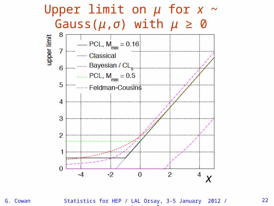
Conditional coverage for CLs, F-C

G. Cowan Statistics for HEP / LAL Orsay, 3-5 January 2012 / Lecture 3 33
The Look-Elsewhere EffectGross and Vitells, EPJC 70:525-530,2010, arXiv:1005.1891
Suppose a model for a mass distribution allows for a peak ata mass m with amplitude μ
The data show a bump at a mass m0.
How consistent is this with the no-bump (μ = 0) hypothesis?
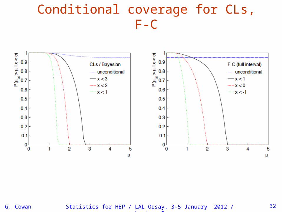
G. Cowan Statistics for HEP / LAL Orsay, 3-5 January 2012 / Lecture 3 34
p-value for fixed massFirst, suppose the mass m0 of the peak was specified a priori.
Test consistency of bump with the no-signal (μ= 0) hypothesis with e.g. likelihood ratio
where “fix” indicates that the mass of the peak is fixed to m0.
The resulting p-value
gives the probability to find a value of tfix at least as great asobserved at the specific mass m0.
Gross and Vitells

G. Cowan Statistics for HEP / LAL Orsay, 3-5 January 2012 / Lecture 3 35
p-value for floating massBut suppose we did not know where in the distribution toexpect a peak.
What we want is the probability to find a peak at least as significant as the one observed anywhere in the distribution.
Include the mass as an adjustable parameter in the fit, test significance of peak using
(Note m does not appearin the μ = 0 model.)
Gross and Vitells

G. Cowan Statistics for HEP / LAL Orsay, 3-5 January 2012 / Lecture 3 36
Distributions of tfix, tfloat
For a sufficiently large data sample, tfix ~chi-square for 1 degreeof freedom (Wilks’ theorem).
For tfloat there are two adjustable parameters, μ and m, and naivelyWilks theorem says tfloat ~ chi-square for 2 d.o.f.
In fact Wilks’ theorem does not hold in the floating mass case because on of the parameters (m) is not-defined in the μ = 0 model.
So getting tfloat distribution is more difficult.
Gross and Vitells

G. Cowan Statistics for HEP / LAL Orsay, 3-5 January 2012 / Lecture 3 37
Trials factorWe would like to be able to relate the p-values for the fixed andfloating mass analyses (at least approximately).
Gross and Vitells show that the “trials factor” can be approximated by
where ‹N› = average number of “upcrossings” of 2lnL in fit range and
is the significance for the fixed mass case.
So we can either carry out the full floating-mass analysis (e.g. use MC to get p-value), or do fixed mass analysis and apply a correction factor (much faster than MC).
Gross and Vitells

G. Cowan Statistics for HEP / LAL Orsay, 3-5 January 2012 / Lecture 3 38
Upcrossings of 2lnLThe Gross-Vitells formula for the trials factor requires themean number “upcrossings” of 2ln L in the fit range basedon fixed threshold.
estimate with MCat low referencelevel
Gross and Vitells

39G. Cowan
Multidimensional look-elsewhere effectGeneralization to multiple dimensions: number of upcrossingsreplaced by expectation of Euler characteristic:
Applications: astrophysics (coordinates on sky), search forresonance of unknown mass and width, ...
Statistics for HEP / LAL Orsay, 3-5 January 2012 / Lecture 3
Vitells and Gross, arXiv:1105.4355

Remember the Look-Elsewhere Effect is when we test a singlemodel (e.g., SM) with multiple observations, i..e, in mulitpleplaces.
Note there is no look-elsewhere effect when consideringexclusion limits. There we test specific signal models (typicallyonce) and say whether each is excluded.
With exclusion there is, however, the analogous issue of testing many signal models (or parameter values) and thus excluding some even in the absence of signal (“spurious exclusion”)
Approximate correction for LEE should be sufficient, and one should also report the uncorrected significance.
“There's no sense in being precise when you don't even know what you're talking about.” –– John von Neumann
40G. Cowan
Summary on Look-Elsewhere Effect
Statistics for HEP / LAL Orsay, 3-5 January 2012 / Lecture 3

Common practice in HEP has been to claim a discovery if the p-value of the no-signal hypothesis is below 2.9 × 10⁷, corresponding to a significance Z = Φ1 (1 – p) = 5 (a 5σ effect).
There a number of reasons why one may want to require sucha high threshold for discovery:
The “cost” of announcing a false discovery is high.
Unsure about systematics.
Unsure about look-elsewhere effect.
The implied signal may be a priori highly improbable(e.g., violation of Lorentz invariance).
41G. Cowan
Why 5 sigma?
Statistics for HEP / LAL Orsay, 3-5 January 2012 / Lecture 3

But the primary role of the p-value is to quantify the probabilitythat the background-only model gives a statistical fluctuationas big as the one seen or bigger.
It is not intended as a means to protect against hidden systematicsor the high standard required for a claim of an important discovery.
In the processes of establishing a discovery there comes a pointwhere it is clear that the observation is not simply a fluctuation,but an “effect”, and the focus shifts to whether this is new physicsor a systematic.
Providing LEE is dealt with, that threshold is probably closer to3σ than 5σ.
42G. Cowan
Why 5 sigma (cont.)?
Statistics for HEP / LAL Orsay, 3-5 January 2012 / Lecture 3

G. Cowan Statistics for HEP / LAL Orsay, 3-5 January 2012 / Lecture 3 43
Summary for first three lectures
Using a frequentist statistical test we can:test the background-only model (rejection = discovery),test possible signal models (rejection leads to limits).
For large enough data sample, approximate formulae allow foreasy evaluation of discovery/exclusion significance.
The important properties of limits include:specified probability to cover true parameter.
Bayesian approach extends probability to degree of belief,and also produce intervals with good frequentist properties.
We saw in the Poisson example that with a one-sided test,all parameter values can be excluded (null interval). We will return to this point on Friday.

G. Cowan Statistics for HEP / LAL Orsay, 3-5 January 2012 / Lecture 3 44
Summary and conclusionsExclusion limits effectively tell one what parameter values are(in)compatible with the data.
Frequentist: exclude range where p-value of param < 5%.Bayesian: low prob. to find parameter in excluded region.
In both cases one must choose the grounds on which the parameteris excluded (estimator too high, low? low likelihood ratio?) .
With a “usual” upper limit, a large downward fluctuationcan lead to exclusion of parameter values to which one haslittle or no sensitivity (will happen 5% of the time).
“Solutions”: CLs, PCL, F-C
All of the solutions have well-defined properties, to whichthere may be some subjective assignment of importance.
G. Cowan Statistics for HEP / LAL Orsay, 3-5 January 2012 / Lecture 3 45
Extra slides

G. Cowan Statistics for HEP / LAL Orsay, 3-5 January 2012 / Lecture 3 46
Coverage probability of intervals for Poisson meanProbability for interval to cover s as function of s(note effect of Poisson discreteness).

Reference priorsJ. Bernardo,L. Demortier,M. PieriniMaximize the expected Kullback–Leibler
divergence of posterior relative to prior:
This maximizes the expected posterior information about θ when the prior density is π(θ).
Finding reference priors “easy” for one parameter:
G. Cowan 47Statistics for HEP / LAL Orsay, 3-5 January 2012 / Lecture 3
(PHYSTAT 2011)

Reference priors (2)J. Bernardo,L. Demortier,M. Pierini
Actual recipe to find reference prior nontrivial;see references from Bernardo’s talk, website ofBerger (www.stat.duke.edu/~berger/papers) and also Demortier, Jain, Prosper, PRD 82:33, 34002 arXiv:1002.1111:
Prior depends on order of parameters. (Is order dependence important? Symmetrize? Sample result from different orderings?)
G. Cowan 48Statistics for HEP / LAL Orsay, 3-5 January 2012 / Lecture 3
(PHYSTAT 2011)

L. Demortier
G. Cowan 49Statistics for HEP / LAL Orsay, 3-5 January 2012 / Lecture 3
(PHYSTAT 2011)
50G. Cowan
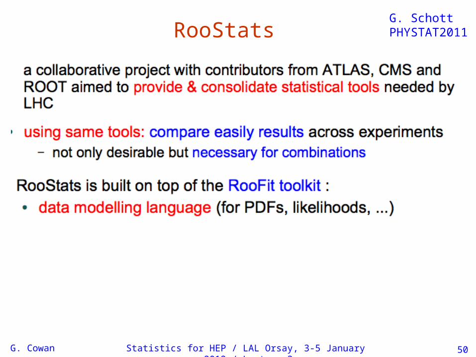
RooStatsG. SchottPHYSTAT2011
Statistics for HEP / LAL Orsay, 3-5 January 2012 / Lecture 3

51G. Cowan
RooFit Workspaces
Able to construct full likelihood for combination of channels(or experiments).
Statistics for HEP / LAL Orsay, 3-5 January 2012 / Lecture 3
G. SchottPHYSTAT2011

Statistics for HEP / LAL Orsay, 3-5 January 2012 / Lecture 352G. Cowan
Combined ATLAS/CMS Higgs searchK. CranmerPHYSTAT2011
Given p-values p1,..., pN of H, what is combined p?
Better, given the results of N (usually independent) experiments, what inferences can one draw from their combination?
Full combination is difficult but worth the effort for e.g. Higgs search.

G. Cowan Statistics for HEP / LAL Orsay, 3-5 January 2012 / Lecture 3 53
PCL for upper limit with Gaussian measurement
Suppose ~ Gauss(μ, σ), goal is to set upper limit on μ.
Define critical region for test of μ as
This gives (unconstrained) upper limit:
inverse of standard Gaussian cumulative distribution

G. Cowan Statistics for HEP / LAL Orsay, 3-5 January 2012 / Lecture 3 54
Power M0(μ) for Gaussian measurement
The power of the test of μ with respect to the alternative μ′ = 0 is:
standard Gaussiancumulative distribution

G. Cowan Statistics for HEP / LAL Orsay, 3-5 January 2012 / Lecture 3 55
Spurious exclusion when μ fluctuates down
Requiring the power be at least Mmin
implies that the smallest μ to which one is sensitive is
If one were to use the unconstrained limit, values of μ at or below μmin would be excluded if
^
That is, one excludes μ < μmin when the unconstrained limit fluctuates too far downward.

G. Cowan Statistics for HEP / LAL Orsay, 3-5 January 2012 / Lecture 3 56
Treatment of nuisance parametersIn most problems, the data distribution is not uniquely specifiedby μ but contains nuisance parameters θ.
This makes it more difficult to construct an (unconstrained)interval with correct coverage probability for all values of θ,so sometimes approximate methods used (“profile construction”).
More importantly for PCL, the power M0(μ) can depend on θ.So which value of θ to use to define the power?
Since the power represents the probability to reject μ if thetrue value is μ = 0, to find the distribution of μup we take the values of θ that best agree with the data for μ = 0:May seem counterintuitive, since the measure of sensitivitynow depends on the data. We are simply using the data to choosethe most appropriate value of θ where we quote the power.

G. Cowan Statistics for HEP / LAL Orsay, 3-5 January 2012 / Lecture 3 57
Flip-flopping
F-C pointed out that if one decides, based on the data, whether to report a one- or two-sided limit, then the stated coverage probability no longer holds.
The problem (flip-flopping) is avoided in unified intervals.
Whether the interval covers correctly or not depends on how one defines repetition of the experiment (the ensemble).
Need to distinguish between:
(1) an idealized ensemble;
(2) a recipe one follows in real life that resembles (1).

G. Cowan Statistics for HEP / LAL Orsay, 3-5 January 2012 / Lecture 3 58
Flip-floppingOne could take, e.g.:
Ideal: always quote upper limit (∞ # of experiments).
Real: quote upper limit for as long as it is of any interest, i.e., until the existence of the effect is well established.
The coverage for the idealized ensemble is correct.
The question is whether the real ensemble departs from this during the period when the limit is of any interest as a guidein the search for the signal.
Here the real and ideal only come into serious conflict if youthink the effect is well established (e.g. at the 5 sigma level)but then subsequently you find it not to be well established,so you need to go back to quoting upper limits.
G. Cowan Statistics for HEP / LAL Orsay, 3-5 January 2012 / Lecture 3 59
Flip-flopping
In an idealized ensemble, this situation could arise if, e.g.,we take x ~ Gauss(μ, σ), and the true μ is one sigmabelow what we regard as the threshold needed to discoverthat μ is nonzero.
Here flip-flopping gives undercoverage because one continually bounces above and below the discovery threshold. The effect keeps going in and out of a state of being established.
But this idealized ensemble does not resemble what happensin reality, where the discovery sensitivity continues to improveas more data are acquired.