Embed Size (px)
DESCRIPTION
G. Cowan Likelihood Workshop, CERN, Jan Quick review of probablility
Citation preview
G. Cowan Likelihood Workshop, CERN, 21-23 Jan 2013 1
Introduction to Likelihoods
Likelihood Workshop
CERN, 21-23, 2013
Glen CowanPhysics DepartmentRoyal Holloway, University of [email protected]/~cowan
http://indico.cern.ch/conferenceDisplay.py?confId=218693
G. Cowan Likelihood Workshop, CERN, 21-23 Jan 2013 2
Outline
I. Introduction and basic formalism
II. Nuisance parameters
III. Frequentist use of likelihoods
IV. Bayesian use of likelihoods
V. “Correlated systematics”
VI. Examples
G. Cowan Likelihood Workshop, CERN, 21-23 Jan 2013 3
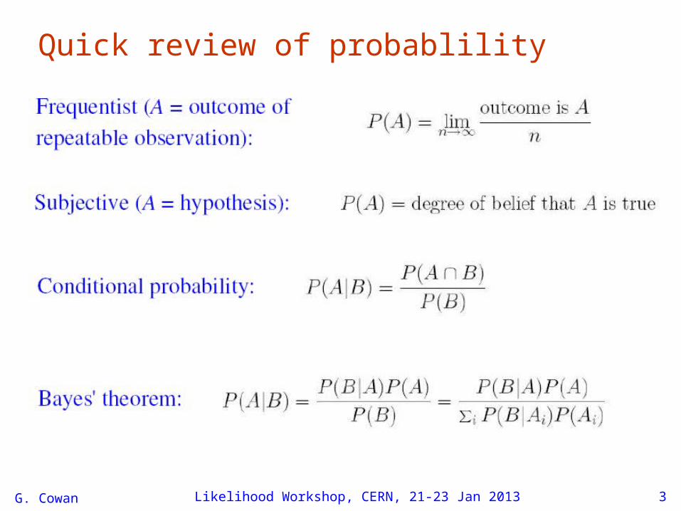
Quick review of probablility
G. Cowan Likelihood Workshop, CERN, 21-23 Jan 2013 4
Frequentist Statistics − general philosophy In frequentist statistics, probabilities are associated only withthe data, i.e., outcomes of repeatable observations.
Probability = limiting frequency
Probabilities such as
P (Higgs boson exists), P (0.117 < s < 0.121),
etc. are either 0 or 1, but we don’t know which.The tools of frequentist statistics tell us what to expect, underthe assumption of certain probabilities, about hypotheticalrepeated observations.
The preferred theories (models, hypotheses, ...) are those for which our observations would be considered ‘usual’.
G. Cowan Likelihood Workshop, CERN, 21-23 Jan 2013 5
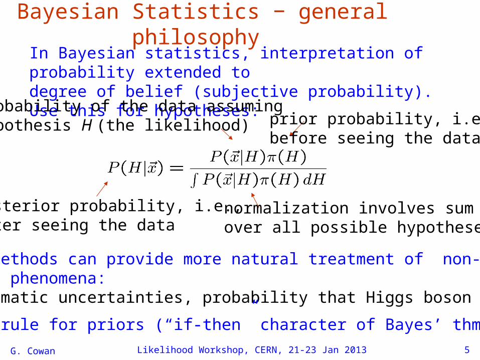
Bayesian Statistics − general philosophy In Bayesian statistics, interpretation of probability extended todegree of belief (subjective probability). Use this for hypotheses:
posterior probability, i.e., after seeing the data
prior probability, i.e.,before seeing the data
probability of the data assuming hypothesis H (the likelihood)
normalization involves sum over all possible hypotheses
Bayesian methods can provide more natural treatment of non-repeatable phenomena: systematic uncertainties, probability that Higgs boson exists,...
No golden rule for priors (“if-then” character of Bayes’ thm.)
G. Cowan Likelihood Workshop, CERN, 21-23 Jan 2013 6
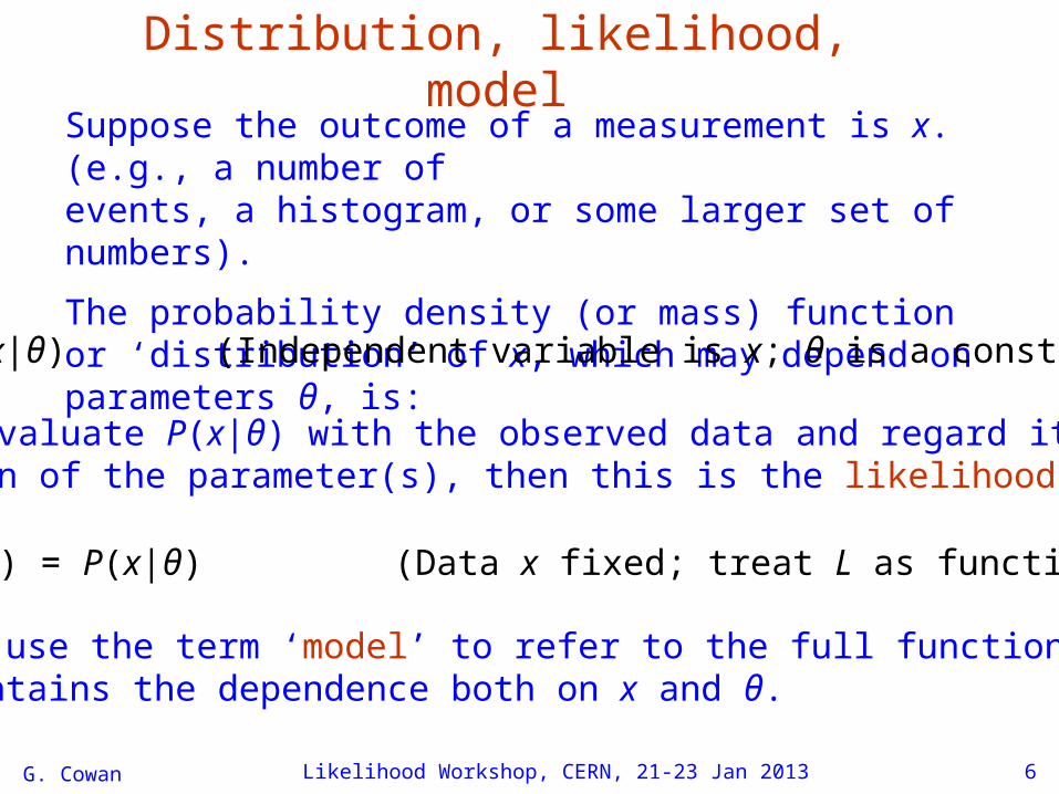
Distribution, likelihood, modelSuppose the outcome of a measurement is x. (e.g., a number of events, a histogram, or some larger set of numbers).
The probability density (or mass) function or ‘distribution’ of x, which may depend on parameters θ, is:
P(x|θ) (Independent variable is x; θ is a constant.)
If we evaluate P(x|θ) with the observed data and regard it as afunction of the parameter(s), then this is the likelihood:
We will use the term ‘model’ to refer to the full function P(x|θ)that contains the dependence both on x and θ.
L(θ) = P(x|θ) (Data x fixed; treat L as function of θ.)
G. Cowan Likelihood Workshop, CERN, 21-23 Jan 2013 7
Bayesian use of the term ‘likelihood’
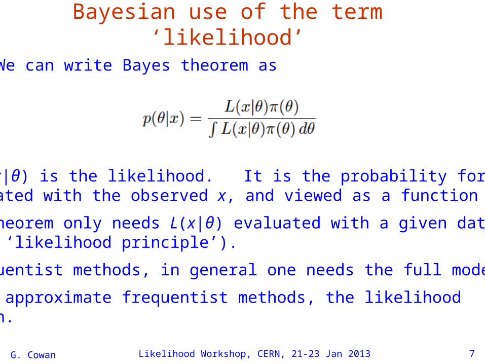
We can write Bayes theorem as
where L(x|θ) is the likelihood. It is the probability for x givenθ, evaluated with the observed x, and viewed as a function of θ.
Bayes’ theorem only needs L(x|θ) evaluated with a given data set (the ‘likelihood principle’).
For frequentist methods, in general one needs the full model.
For some approximate frequentist methods, the likelihood is enough.
G. Cowan Likelihood Workshop, CERN, 21-23 Jan 2013 8
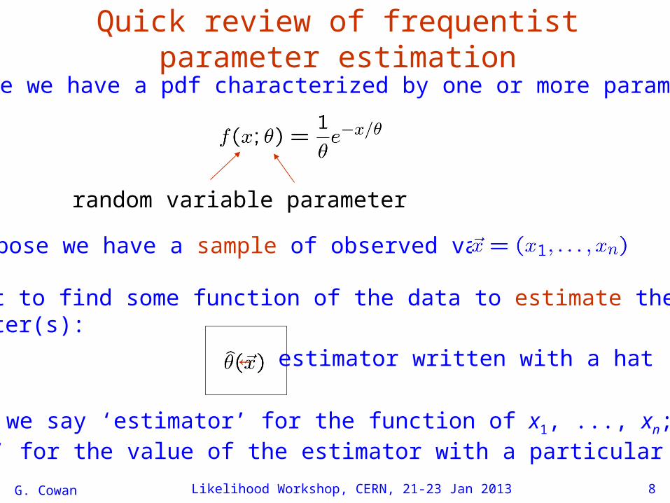
Quick review of frequentist parameter estimationSuppose we have a pdf characterized by one or more parameters:
random variable
Suppose we have a sample of observed values:
parameter
We want to find some function of the data to estimate the parameter(s):
← estimator written with a hat
Sometimes we say ‘estimator’ for the function of x1, ..., xn;‘estimate’ for the value of the estimator with a particular data set.
G. Cowan Likelihood Workshop, CERN, 21-23 Jan 2013 9
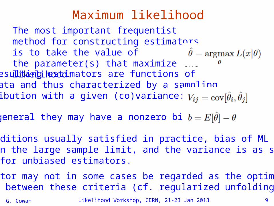
Maximum likelihoodThe most important frequentist method for constructing estimators is to take the value of the parameter(s) that maximize the likelihood:
The resulting estimators are functions of the data and thus characterized by a sampling distribution with a given (co)variance:
In general they may have a nonzero bias:
Under conditions usually satisfied in practice, bias of ML estimatorsis zero in the large sample limit, and the variance is as small aspossible for unbiased estimators.
ML estimator may not in some cases be regarded as the optimal trade-off between these criteria (cf. regularized unfolding).
G. Cowan Likelihood Workshop, CERN, 21-23 Jan 2013 10
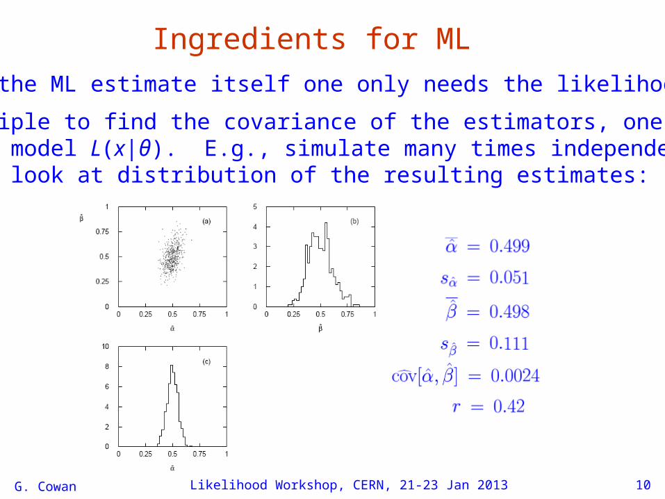
Ingredients for MLTo find the ML estimate itself one only needs the likelihood L(θ) .
In principle to find the covariance of the estimators, one requiresthe full model L(x|θ). E.g., simulate many times independent data sets and look at distribution of the resulting estimates:
G. Cowan Likelihood Workshop, CERN, 21-23 Jan 2013 11
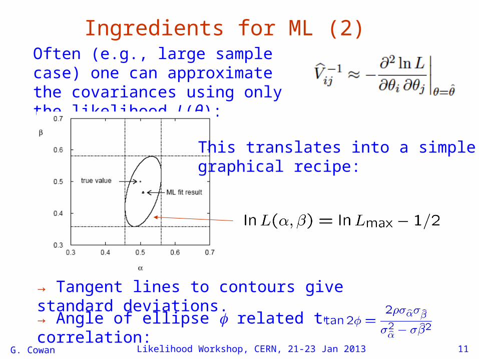
Ingredients for ML (2)Often (e.g., large sample case) one can approximate the covariances using only the likelihood L(θ):
→ Tangent lines to contours give standard deviations.
→ Angle of ellipse related to correlation:
This translates into a simplegraphical recipe:
G. Cowan Likelihood Workshop, CERN, 21-23 Jan 2013 12
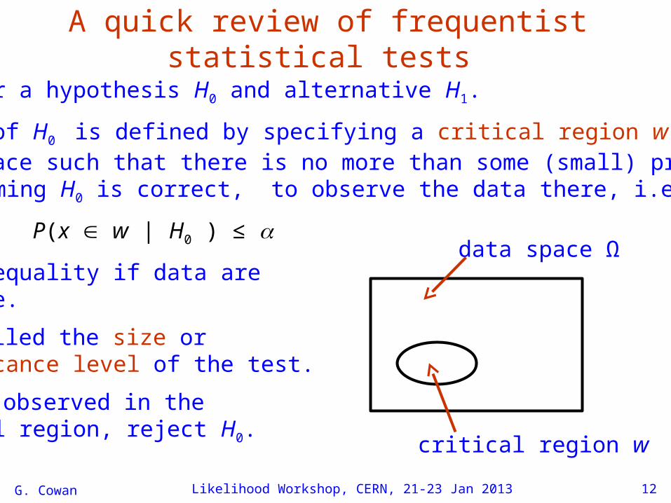
A quick review of frequentist statistical tests
Consider a hypothesis H0 and alternative H1.
A test of H0 is defined by specifying a critical region w of thedata space such that there is no more than some (small) probability, assuming H0 is correct, to observe the data there, i.e.,
P(x w | H0 ) ≤
Need inequality if data arediscrete.
α is called the size or significance level of the test.
If x is observed in the critical region, reject H0.
data space Ω
critical region w
G. Cowan Likelihood Workshop, CERN, 21-23 Jan 2013 13
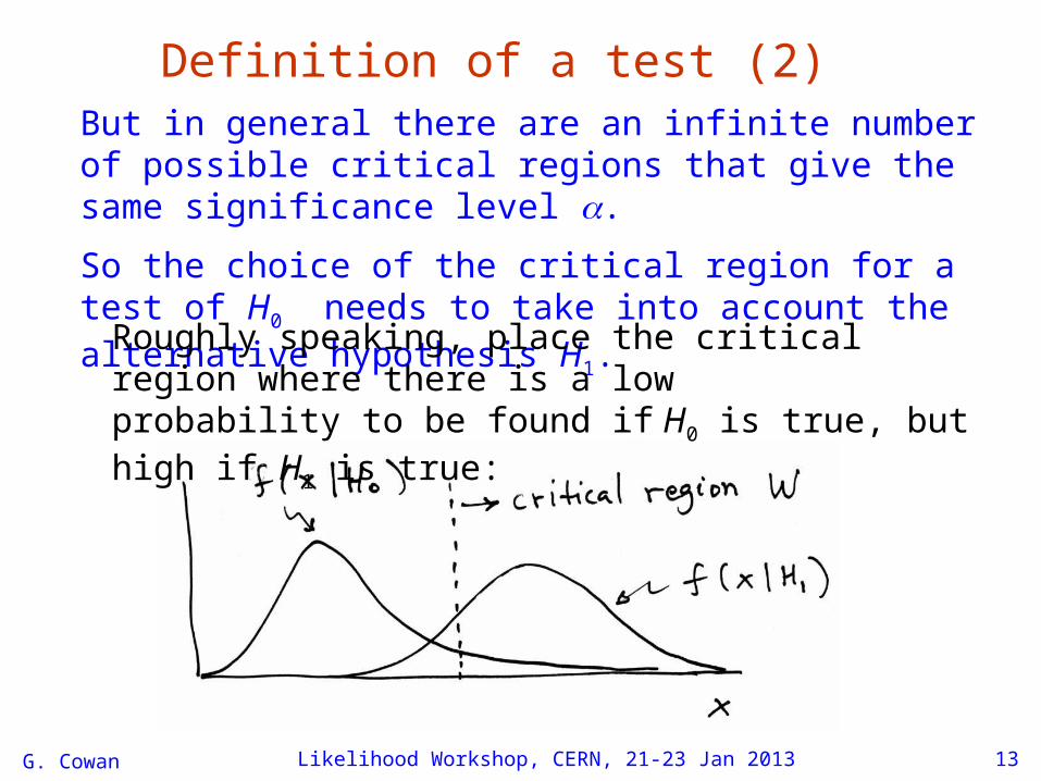
Definition of a test (2)But in general there are an infinite number of possible critical regions that give the same significance level .
So the choice of the critical region for a test of H0 needs to take into account the alternative hypothesis H1.
Roughly speaking, place the critical region where there is a low probability to be found if H0 is true, but high if H1 is true:
G. Cowan Likelihood Workshop, CERN, 21-23 Jan 2013 14
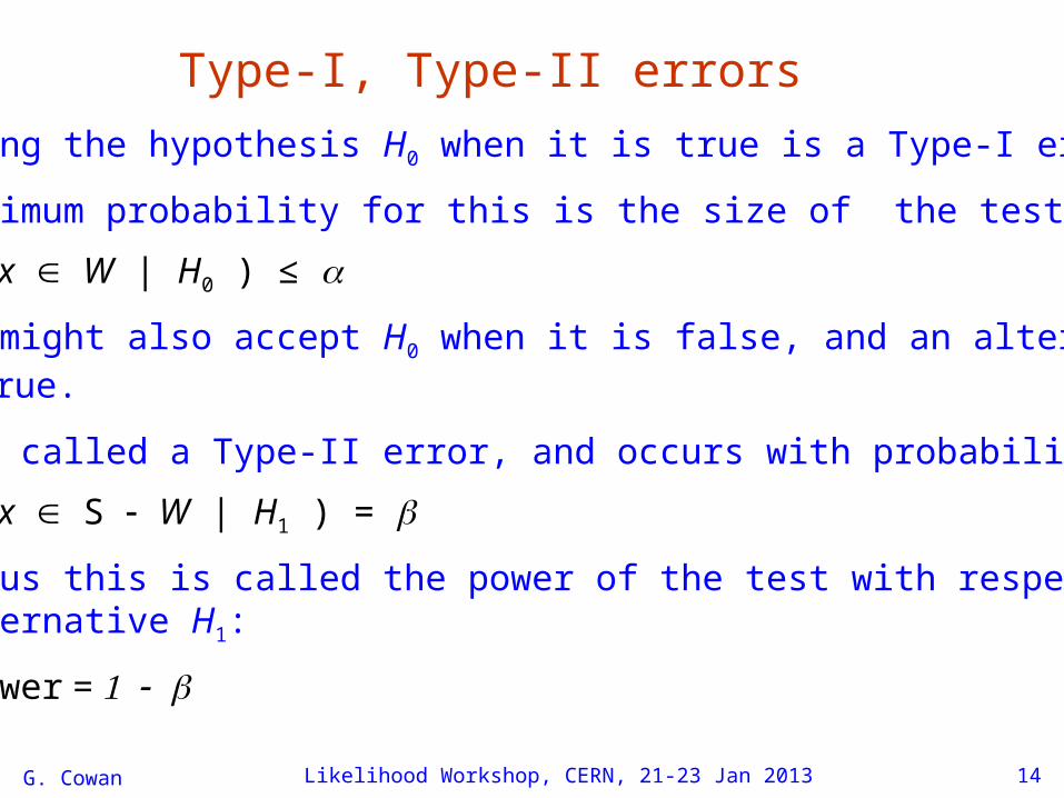
Type-I, Type-II errors Rejecting the hypothesis H0 when it is true is a Type-I error.
The maximum probability for this is the size of the test:
P(x W | H0 ) ≤
But we might also accept H0 when it is false, and an alternative H1 is true.
This is called a Type-II error, and occurs with probability
P(x S W | H1 ) =
One minus this is called the power of the test with respect tothe alternative H1:
Power =
Likelihood Workshop, CERN, 21-23 Jan 2013 15
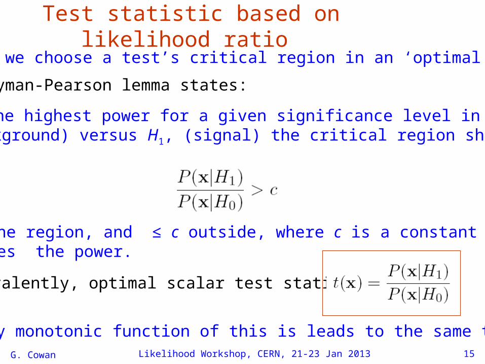
Test statistic based on likelihood ratio How can we choose a test’s critical region in an ‘optimal way’?
Neyman-Pearson lemma states:
To get the highest power for a given significance level in a test ofH0, (background) versus H1, (signal) the critical region should have
inside the region, and ≤ c outside, where c is a constant which determines the power.
Equivalently, optimal scalar test statistic is
N.B. any monotonic function of this is leads to the same test.G. Cowan
G. Cowan Likelihood Workshop, CERN, 21-23 Jan 2013 16
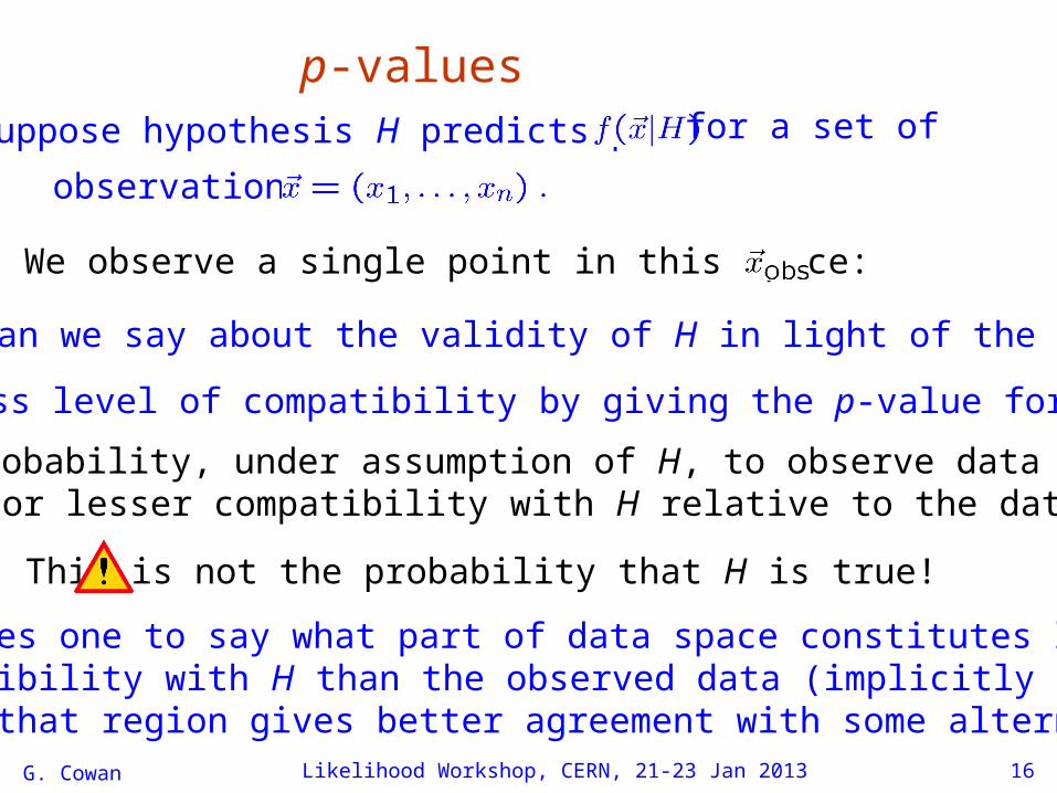
p-valuesSuppose hypothesis H predicts pdf observations
for a set of
We observe a single point in this space:
What can we say about the validity of H in light of the data?
Express level of compatibility by giving the p-value for H:
p = probability, under assumption of H, to observe data with equal or lesser compatibility with H relative to the data we got.
This is not the probability that H is true!
Requires one to say what part of data space constitutes lessercompatibility with H than the observed data (implicitly thismeans that region gives better agreement with some alternative).
G. Cowan 17
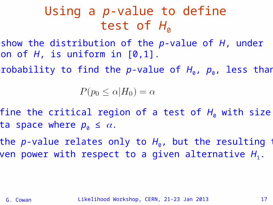
Using a p-value to define test of H0
One can show the distribution of the p-value of H, under assumption of H, is uniform in [0,1].
So the probability to find the p-value of H0, p0, less than is
Likelihood Workshop, CERN, 21-23 Jan 2013
We can define the critical region of a test of H0 with size as the set of data space where p0 ≤ .
Formally the p-value relates only to H0, but the resulting test willhave a given power with respect to a given alternative H1.

G. Cowan Likelihood Workshop, CERN, 21-23 Jan 2013 18
Confidence intervals by inverting a testConfidence intervals for a parameter can be found by defining a test of the hypothesized value (do this for all ):
Specify values of the data that are ‘disfavoured’ by (critical region) such that P(data in critical region) ≤ for a prespecified , e.g., 0.05 or 0.1.
If data observed in the critical region, reject the value .
Now invert the test to define a confidence interval as:
set of values that would not be rejected in a test ofsize (confidence level is 1 ).
The interval will cover the true value of with probability ≥ 1 .
Equivalently, the parameter values in the confidence interval havep-values of at least .
G. Cowan Likelihood Workshop, CERN, 21-23 Jan 2013 19
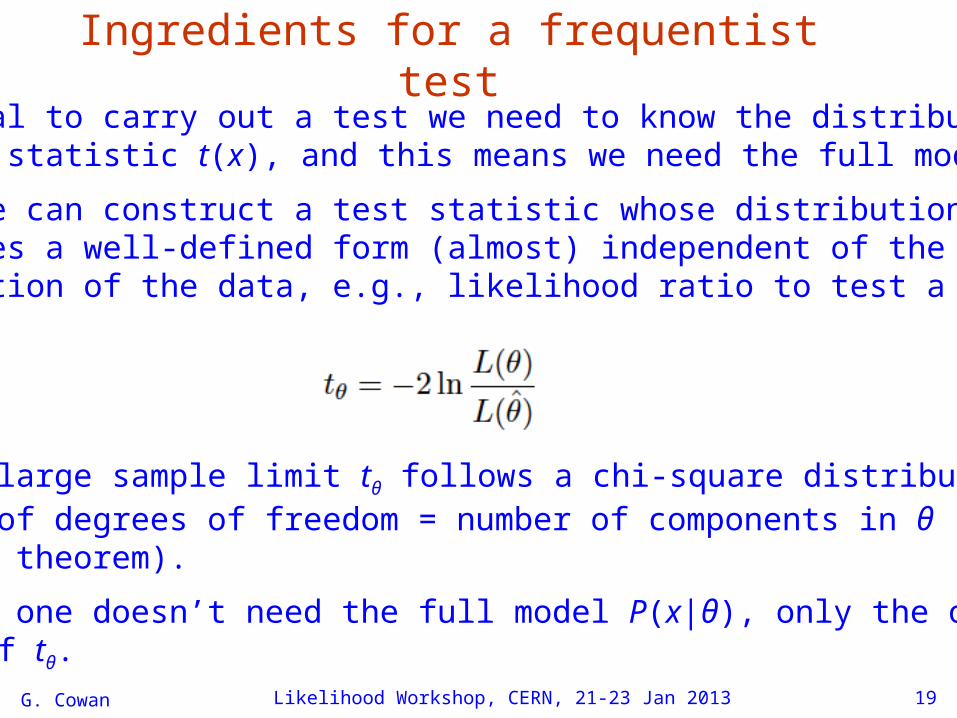
Ingredients for a frequentist testIn general to carry out a test we need to know the distribution of the test statistic t(x), and this means we need the full model P(x|H).
Often one can construct a test statistic whose distribution approaches a well-defined form (almost) independent of the distribution of the data, e.g., likelihood ratio to test a value of θ:
In the large sample limit tθ follows a chi-square distribution withnumber of degrees of freedom = number of components in θ(Wilks’ theorem).
So here one doesn’t need the full model P(x|θ), only the observed value of tθ.
G. Cowan Likelihood Workshop, CERN, 21-23 Jan 2013 page 20
Statistical vs. systematic errors Statistical errors:
How much would the result fluctuate upon repetition of the measurement?
Implies some set of assumptions to define probability of outcome of the measurement.
Systematic errors:
What is the uncertainty in my result due to uncertainty in my assumptions, e.g.,
model (theoretical) uncertainty;modelling of measurement apparatus.
Usually taken to mean the sources of error do not vary upon repetition of the measurement. Often result from uncertain value of calibration constants, efficiencies, etc.
G. Cowan Likelihood Workshop, CERN, 21-23 Jan 2013 21
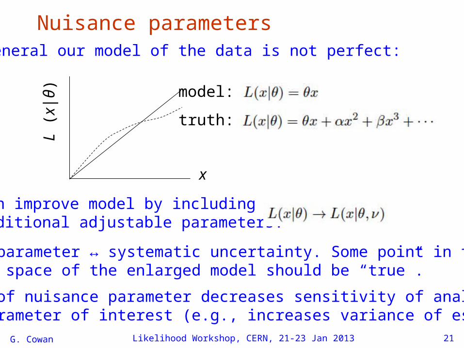
Nuisance parametersIn general our model of the data is not perfect:
x
L (x
|θ) model:
truth:
Can improve model by including additional adjustable parameters.
Nuisance parameter ↔ systematic uncertainty. Some point in theparameter space of the enlarged model should be “true”.
Presence of nuisance parameter decreases sensitivity of analysisto the parameter of interest (e.g., increases variance of estimate).
G. Cowan Likelihood Workshop, CERN, 21-23 Jan 2013 22
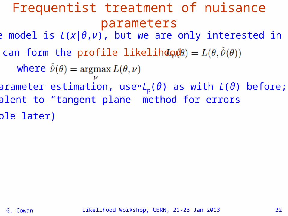
Frequentist treatment of nuisance parametersSuppose model is L(x|θ,ν), but we are only interested in θ.
where
We can form the profile likelihood:
For parameter estimation, use Lp(θ) as with L(θ) before;equivalent to “tangent plane” method for errors
(Example later)
G. Cowan Likelihood Workshop, CERN, 21-23 Jan 2013 23
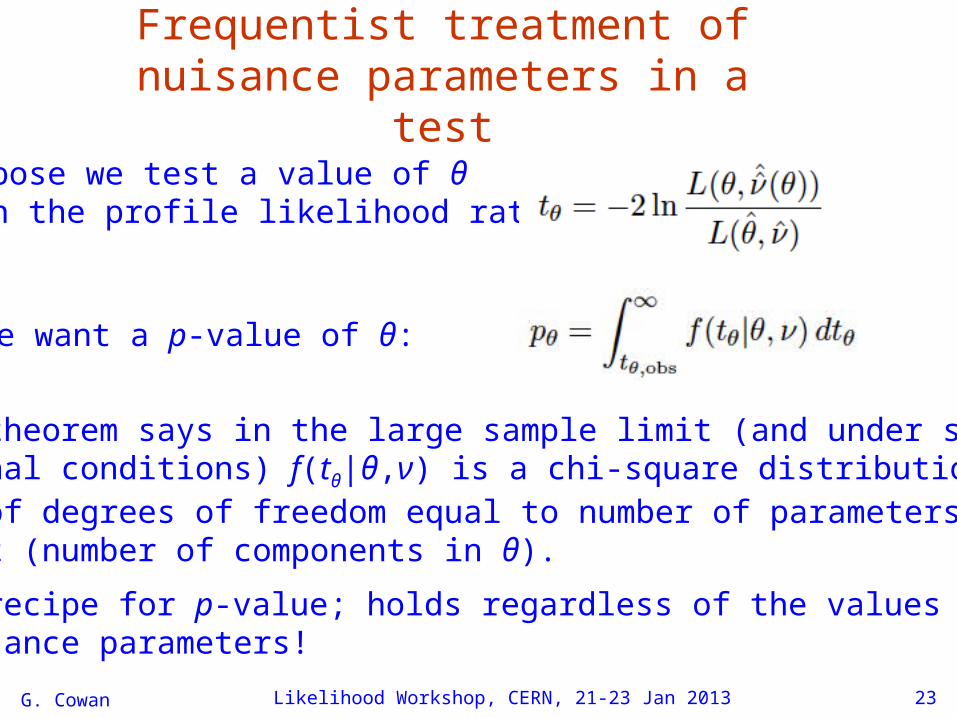
Frequentist treatment of nuisance parameters in a test
Suppose we test a value of θ with the profile likelihood ratio:
We want a p-value of θ:
Wilks’ theorem says in the large sample limit (and under someadditional conditions) f(tθ|θ,ν) is a chi-square distribution withnumber of degrees of freedom equal to number of parameters ofinterest (number of components in θ).
Simple recipe for p-value; holds regardless of the values of the nuisance parameters!
G. Cowan Likelihood Workshop, CERN, 21-23 Jan 2013 24
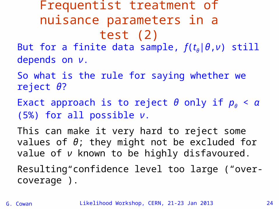
Frequentist treatment of nuisance parameters in a test (2)
But for a finite data sample, f(tθ|θ,ν) still depends on ν.
So what is the rule for saying whether we reject θ?
Exact approach is to reject θ only if pθ < α (5%) for all possible ν.
This can make it very hard to reject some values of θ; they might not be excluded for value of ν known to be highly disfavoured.
Resulting confidence level too large (“over-coverage”).
G. Cowan Likelihood Workshop, CERN, 21-23 Jan 2013 25
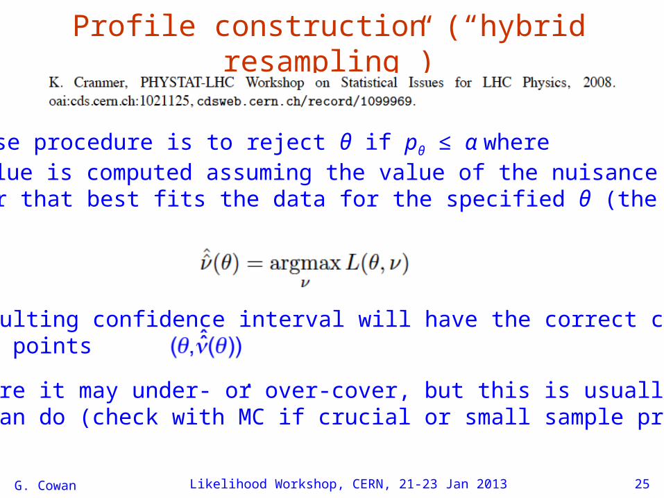
Profile construction (“hybrid resampling”)
Compromise procedure is to reject θ if pθ ≤ α wherethe p-value is computed assuming the value of the nuisanceparameter that best fits the data for the specified θ (the profiledvalues):
The resulting confidence interval will have the correct coveragefor the points
.Elsewhere it may under- or over-cover, but this is usually as goodas we can do (check with MC if crucial or small sample problem).
G. Cowan Likelihood Workshop, CERN, 21-23 Jan 2013 26
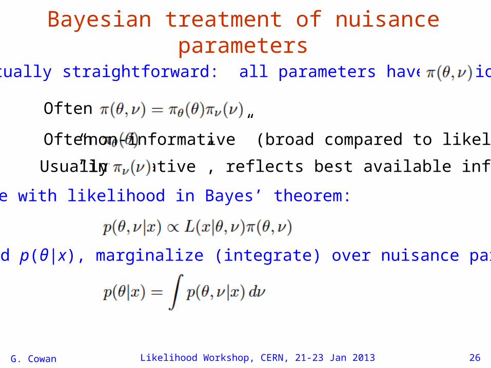
Bayesian treatment of nuisance parameters
Conceptually straightforward: all parameters have a prior:
Often
Often “non-informative” (broad compared to likelihood).
Usually “informative”, reflects best available info. on ν.
Use with likelihood in Bayes’ theorem:
To find p(θ|x), marginalize (integrate) over nuisance param.:

G. Cowan Likelihood Workshop, CERN, 21-23 Jan 2013 page 27
Marginalization with MCMCBayesian computations involve integrals like
often high dimensionality and impossible in closed form,also impossible with ‘normal’ acceptance-rejection Monte Carlo.
Markov Chain Monte Carlo (MCMC) has revolutionizedBayesian computation.
MCMC (e.g., Metropolis-Hastings algorithm) generates correlated sequence of random numbers:
cannot use for many applications, e.g., detector MC;effective stat. error greater than naive √n .
Basic idea: sample full multidimensional parameter space;look, e.g., only at distribution of parameters of interest.
G. Cowan Likelihood Workshop, CERN, 21-23 Jan 2013 28
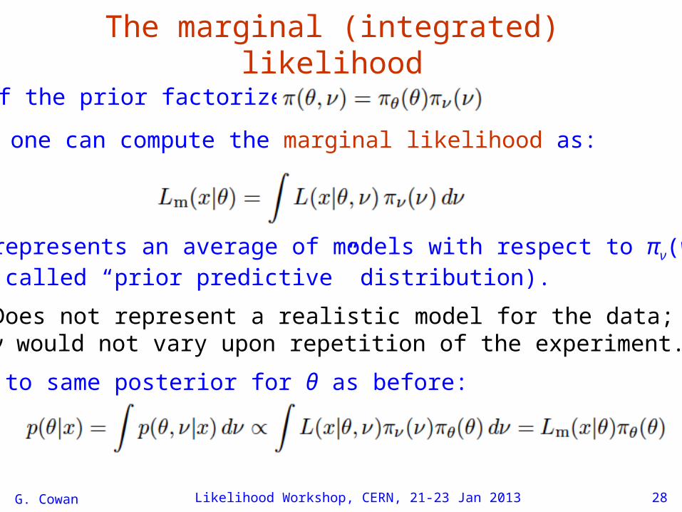
The marginal (integrated) likelihood
If the prior factorizes:
then one can compute the marginal likelihood as:
This represents an average of models with respect to πν(ν)(also called “prior predictive” distribution).
Does not represent a realistic model for the data;ν would not vary upon repetition of the experiment.
Leads to same posterior for θ as before:
G. Cowan Likelihood Workshop, CERN, 21-23 Jan 2013 29
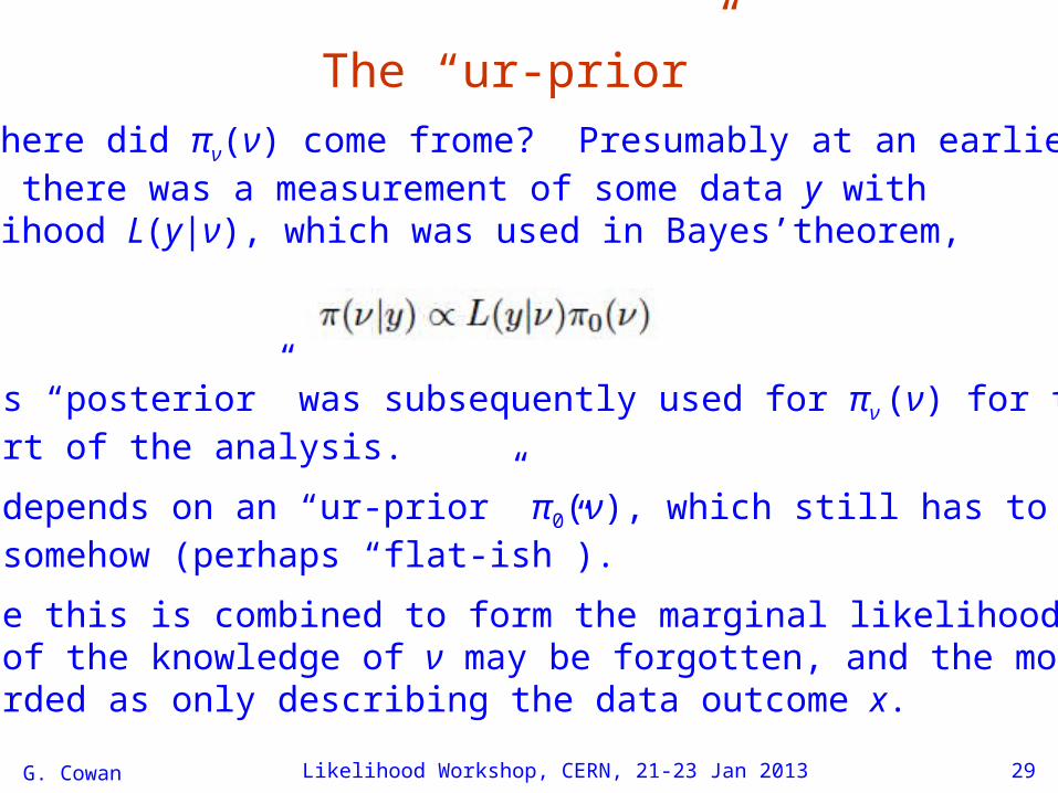
The “ur-prior”But where did πν(ν) come frome? Presumably at an earlierpoint there was a measurement of some data y withlikelihood L(y|ν), which was used in Bayes’theorem,
and this “posterior” was subsequently used for πν (ν) for thenext part of the analysis.
But it depends on an “ur-prior” π0(ν), which still has to bechosen somehow (perhaps “flat-ish”).
But once this is combined to form the marginal likelihood, theorigin of the knowledge of ν may be forgotten, and the modelis regarded as only describing the data outcome x.
G. Cowan Likelihood Workshop, CERN, 21-23 Jan 2013 30
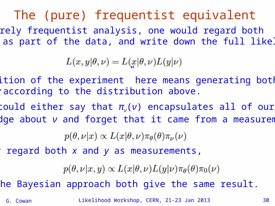
The (pure) frequentist equivalentIn a purely frequentist analysis, one would regard bothx and y as part of the data, and write down the full likelihood:
“Repetition of the experiment” here means generating bothx and y according to the distribution above.
So we could either say that πν(ν) encapsulates all of our prior knowledge about ν and forget that it came from a measurement,
or regard both x and y as measurements,
In the Bayesian approach both give the same result.
G. Cowan Likelihood Workshop, CERN, 21-23 Jan 2013 31
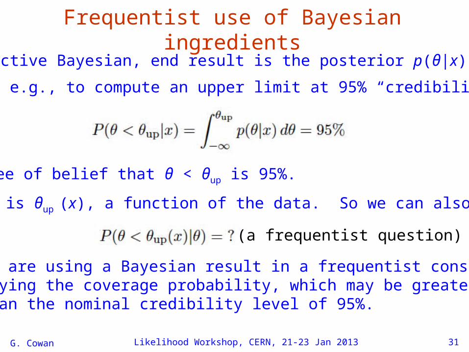
Frequentist use of Bayesian ingredientsFor subjective Bayesian, end result is the posterior p(θ|x).
Use this, e.g., to compute an upper limit at 95% “credibility level”:
→ Degree of belief that θ < θup is 95%.
But θup is θup (x), a function of the data. So we can also ask
(a frequentist question)
Here we are using a Bayesian result in a frequentist construct by studying the coverage probability, which may be greater orless than the nominal credibility level of 95%.
G. Cowan Likelihood Workshop, CERN, 21-23 Jan 2013 32
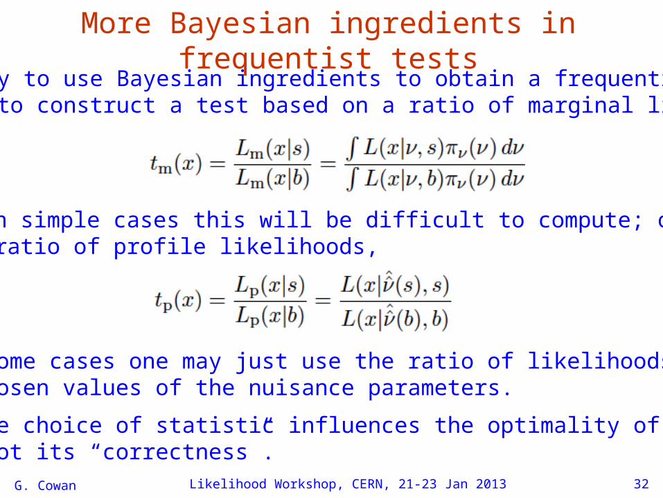
More Bayesian ingredients in frequentist testsAnother way to use Bayesian ingredients to obtain a frequentistresult is to construct a test based on a ratio of marginal likelihoods:
Except in simple cases this will be difficult to compute; often useinstead ratio of profile likelihoods,
or in some cases one may just use the ratio of likelihoods forsome chosen values of the nuisance parameters.
Here the choice of statistic influences the optimality of thetest, not its “correctness”.
G. Cowan Likelihood Workshop, CERN, 21-23 Jan 2013 33
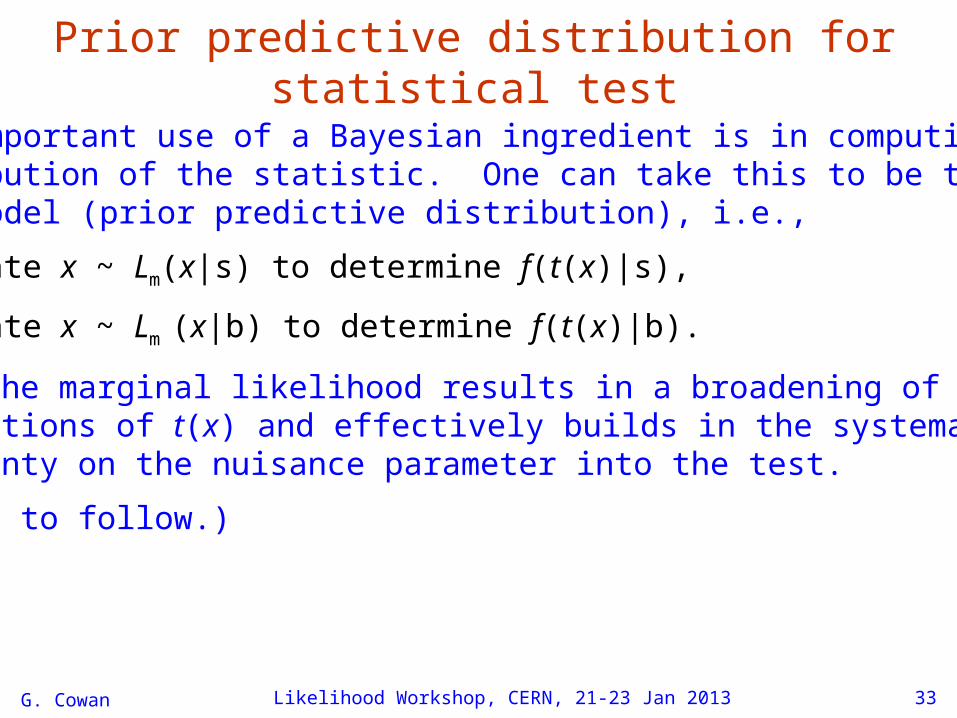
Prior predictive distribution for statistical test
The more important use of a Bayesian ingredient is in computingthe distribution of the statistic. One can take this to be the Bayesianaveraged model (prior predictive distribution), i.e.,
Generate x ~ Lm(x|s) to determine f(t(x)|s),
Generate x ~ Lm (x|b) to determine f(t(x)|b).
Use of the marginal likelihood results in a broadening of thedistributions of t(x) and effectively builds in the systematicuncertainty on the nuisance parameter into the test.
(Example to follow.)
G. Cowan Likelihood Workshop, CERN, 21-23 Jan 2013 34
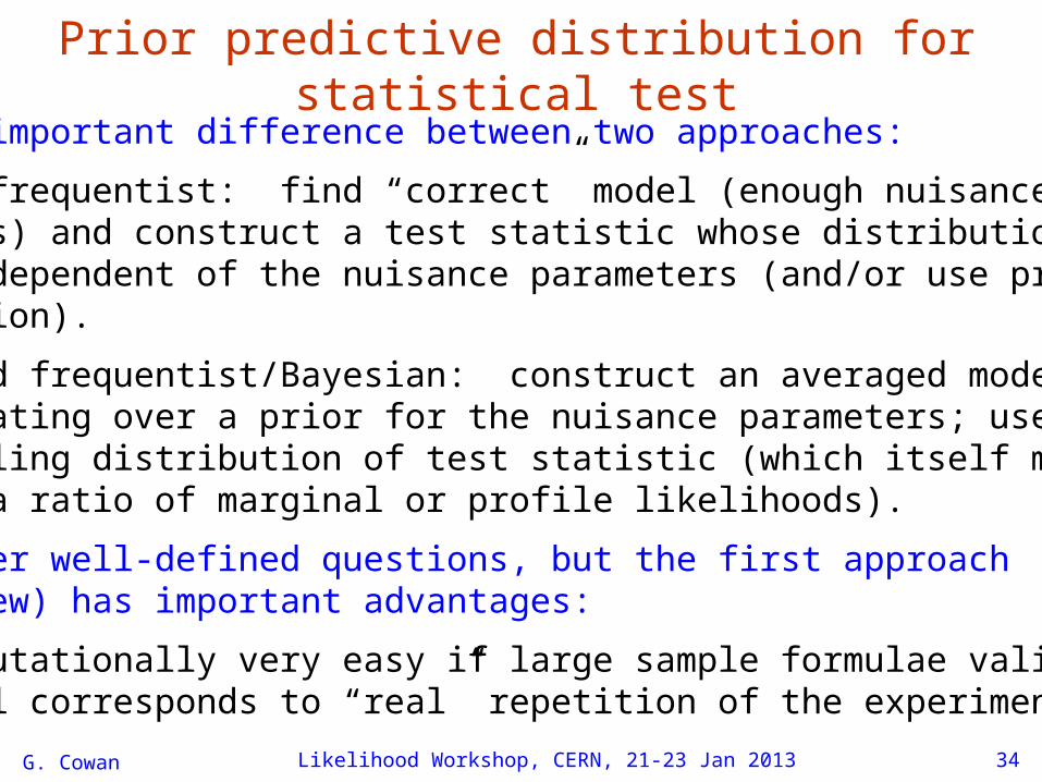
Prior predictive distribution for statistical testNote the important difference between two approaches:
1) Pure frequentist: find “correct” model (enough nuisance parameters) and construct a test statistic whose distribution is almost independent of the nuisance parameters (and/or use profile construction).
2) Hybrid frequentist/Bayesian: construct an averaged model by integrating over a prior for the nuisance parameters; use this to find sampling distribution of test statistic (which itself may bebased on a ratio of marginal or profile likelihoods).
Both answer well-defined questions, but the first approach (in my view) has important advantages:
Computationally very easy if large sample formulae valid;Model corresponds to “real” repetition of the experiment.
G. Cowan Likelihood Workshop, CERN, 21-23 Jan 2013 35
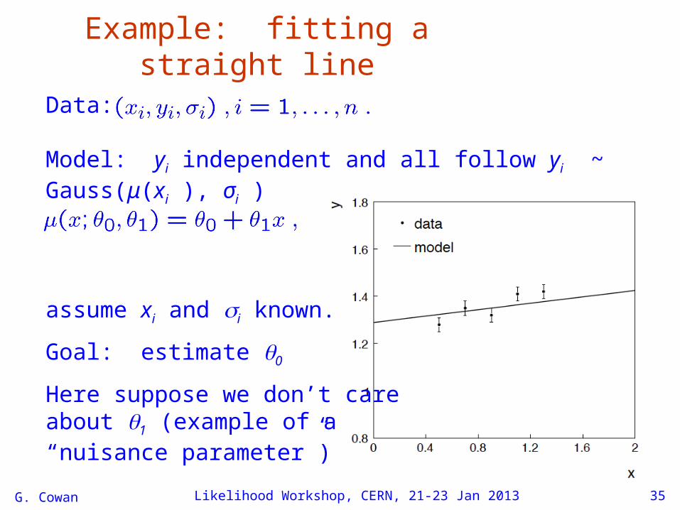
Example: fitting a straight line
Data:
Model: yi independent and all follow yi ~ Gauss(μ(xi ), σi )
assume xi and i known.
Goal: estimate 0
Here suppose we don’t care about 1 (example of a “nuisance parameter”)
G. Cowan Likelihood Workshop, CERN, 21-23 Jan 2013 36
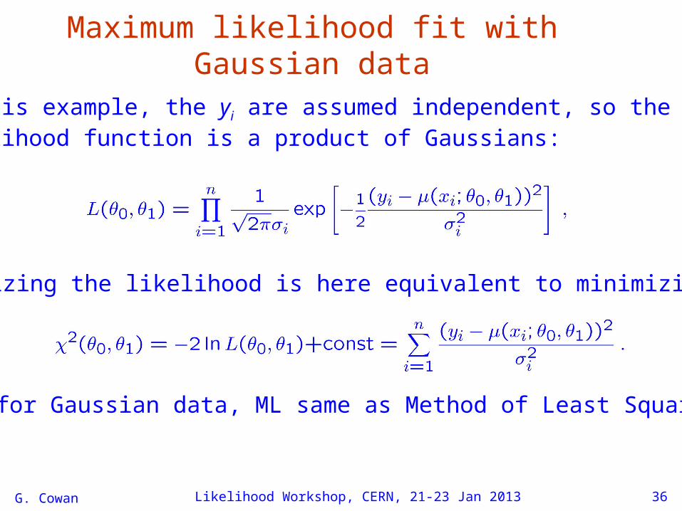
Maximum likelihood fit with Gaussian data
In this example, the yi are assumed independent, so thelikelihood function is a product of Gaussians:
Maximizing the likelihood is here equivalent to minimizing
i.e., for Gaussian data, ML same as Method of Least Squares (LS)
G. Cowan Likelihood Workshop, CERN, 21-23 Jan 2013 37
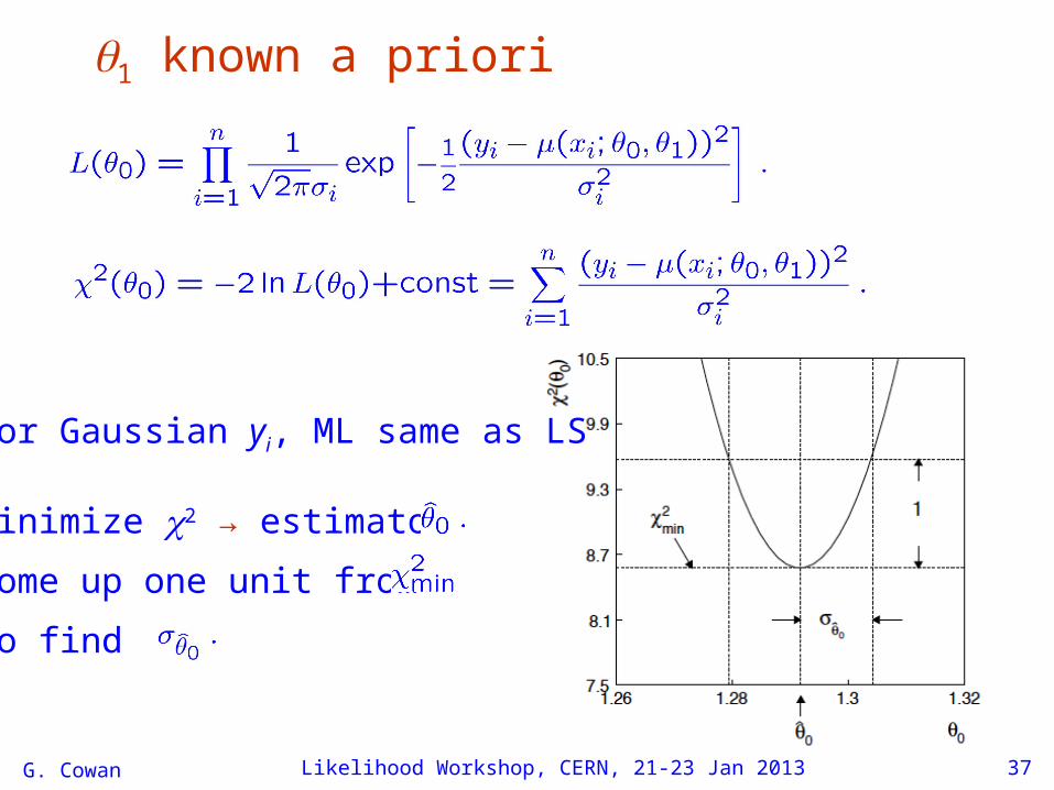
1 known a priori
For Gaussian yi, ML same as LS
Minimize χ2 → estimator
Come up one unit from
to find
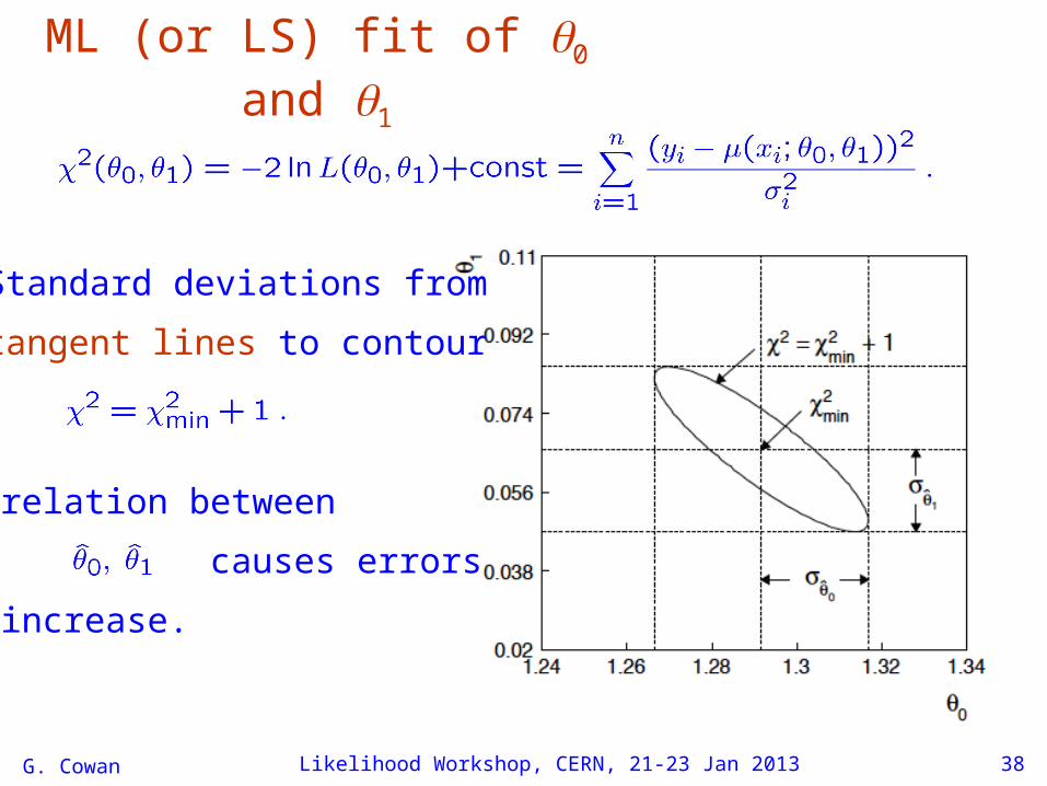
G. Cowan Likelihood Workshop, CERN, 21-23 Jan 2013 38
Correlation between
causes errors
to increase.
Standard deviations from
tangent lines to contour
ML (or LS) fit of 0 and 1
G. Cowan Likelihood Workshop, CERN, 21-23 Jan 2013 39
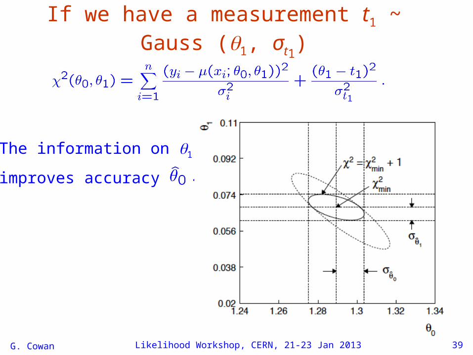
The information on 1
improves accuracy of
If we have a measurement t1 ~ Gauss (1, σt1)
G. Cowan Likelihood Workshop, CERN, 21-23 Jan 2013 40
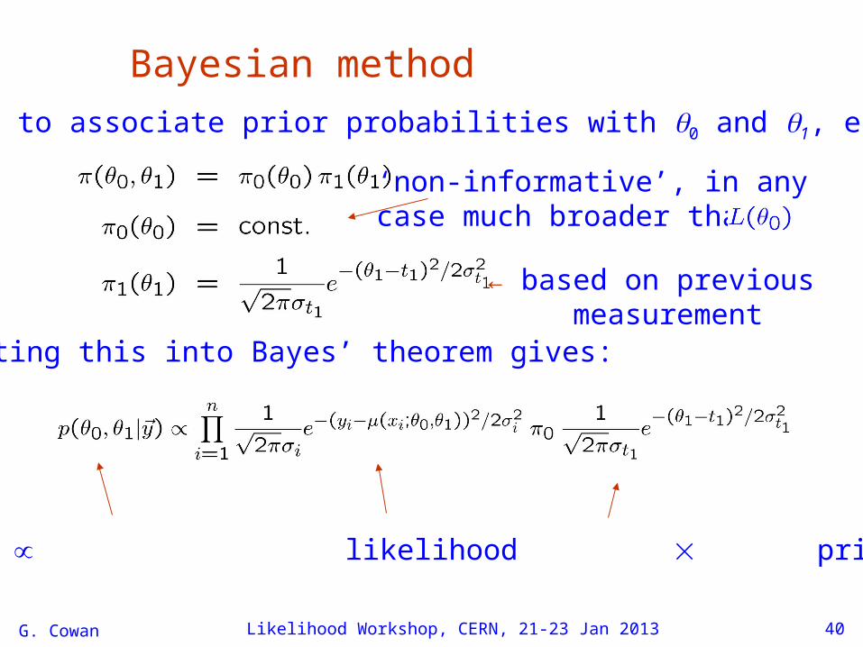
Bayesian methodWe need to associate prior probabilities with 0 and 1, e.g.,
Putting this into Bayes’ theorem gives:
posterior likelihood prior
← based on previous measurement
‘non-informative’, in anycase much broader than
G. Cowan Likelihood Workshop, CERN, 21-23 Jan 2013 41
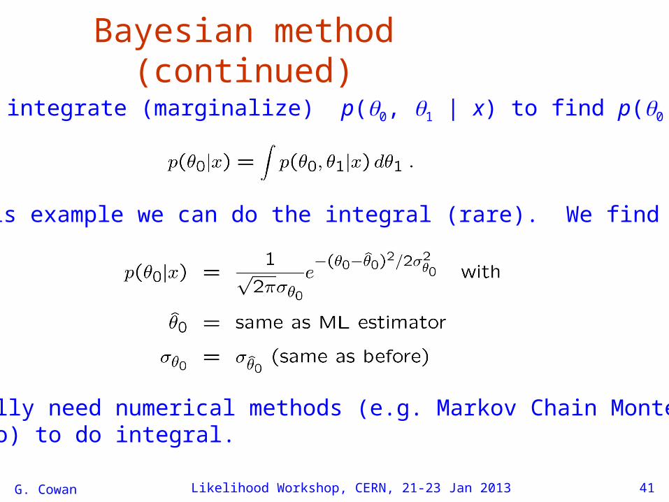
Bayesian method (continued)
Usually need numerical methods (e.g. Markov Chain MonteCarlo) to do integral.
We then integrate (marginalize) p(0, 1 | x) to find p(0 | x):
In this example we can do the integral (rare). We find
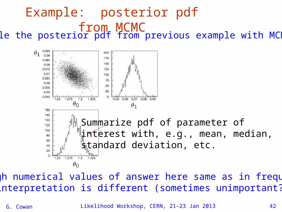
G. Cowan Likelihood Workshop, CERN, 21-23 Jan 2013 42
Although numerical values of answer here same as in frequentistcase, interpretation is different (sometimes unimportant?)
Example: posterior pdf from MCMCSample the posterior pdf from previous example with MCMC:
Summarize pdf of parameter ofinterest with, e.g., mean, median,standard deviation, etc.
G. Cowan Likelihood Workshop, CERN, 21-23 Jan 2013 43
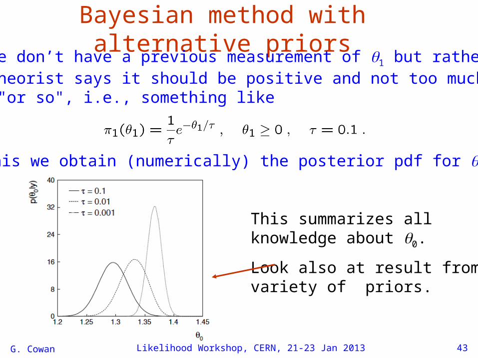
Bayesian method with alternative priorsSuppose we don’t have a previous measurement of 1 but rather, e.g., a theorist says it should be positive and not too much greaterthan 0.1 "or so", i.e., something like
From this we obtain (numerically) the posterior pdf for 0:
This summarizes all knowledge about 0.
Look also at result from variety of priors.
G. Cowan Likelihood Workshop, CERN, 21-23 Jan 2013 44
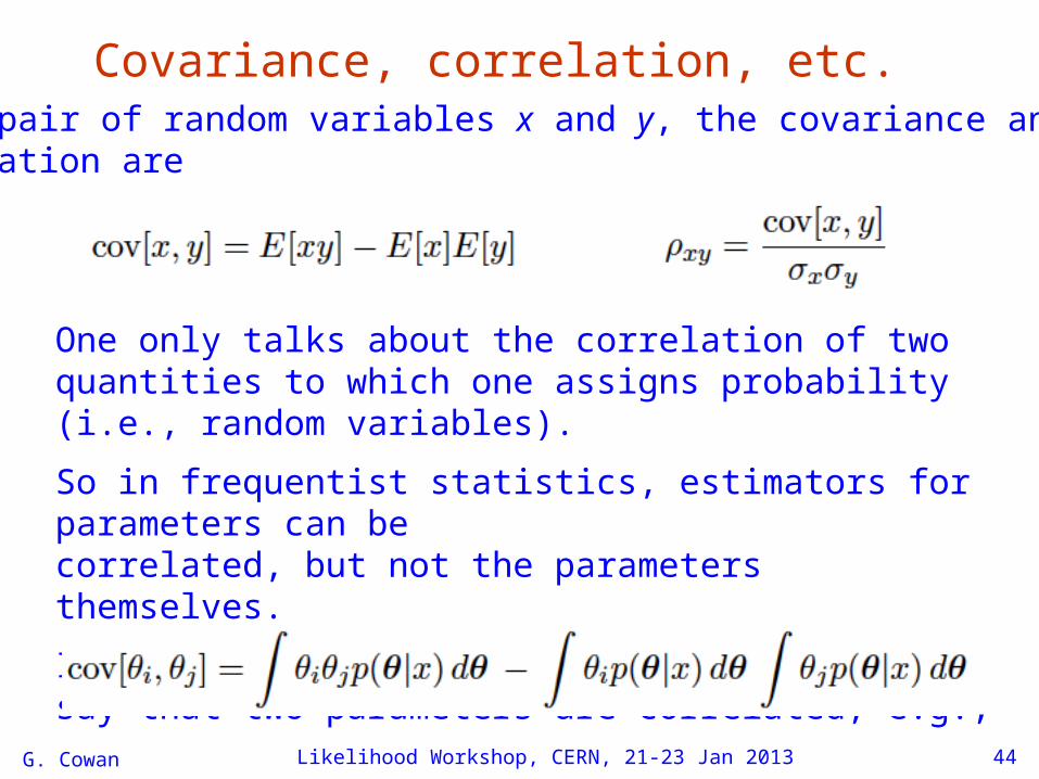
Covariance, correlation, etc.For a pair of random variables x and y, the covariance andcorrelation are
One only talks about the correlation of two quantities to which one assigns probability (i.e., random variables).
So in frequentist statistics, estimators for parameters can becorrelated, but not the parameters themselves.
In Bayesian statistics it does make sense to say that two parameters are correlated, e.g.,
G. Cowan Likelihood Workshop, CERN, 21-23 Jan 2013 45
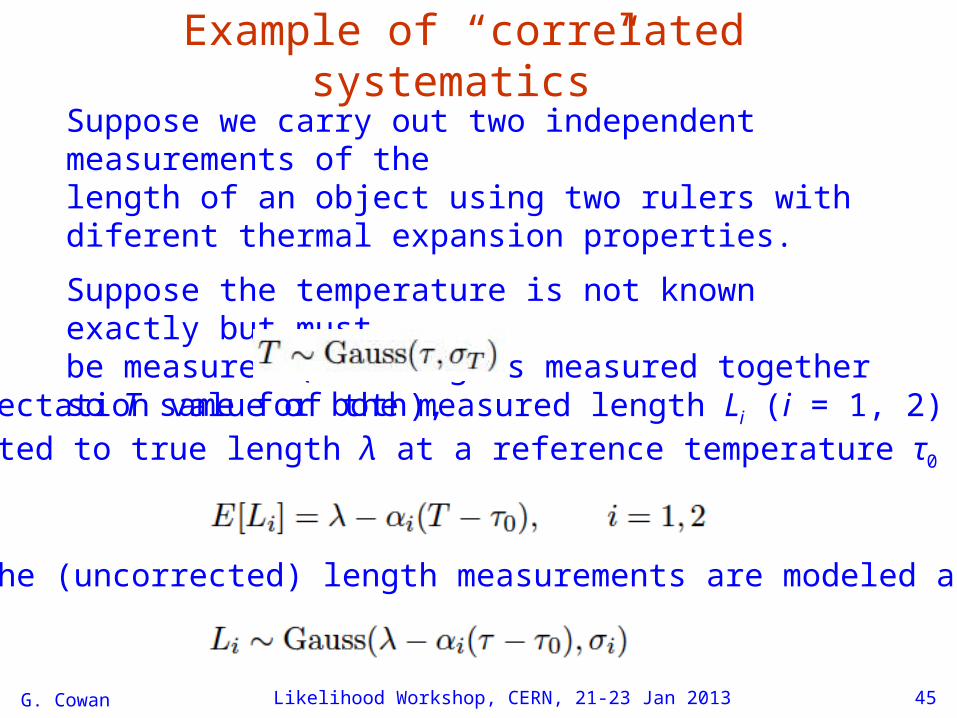
Example of “correlated systematics”Suppose we carry out two independent measurements of the length of an object using two rulers with diferent thermal expansion properties.
Suppose the temperature is not known exactly but mustbe measured (but lengths measured together so T same for both),
and the (uncorrected) length measurements are modeled as
The expectation value of the measured length Li (i = 1, 2) is related to true length λ at a reference temperature τ0 by

G. Cowan Likelihood Workshop, CERN, 21-23 Jan 2013 46
Two rulers (2)The model thus treats the measurements T, L1, L2 as uncorrelated with standard deviations σT, σ1, σ2, respectively:
Alternatively we could correct each raw measurement:
which introduces a correlation between y1, y2 and T
But the likelihood function (multivariate Gauss in T, y1, y2) is the same function of τ and λ as before.
Language of y1, y2: temperature gives correlated systematic. Language of L1, L2: temperature gives “coherent” systematic.
G. Cowan Likelihood Workshop, CERN, 21-23 Jan 2013 47
Two rulers (3)
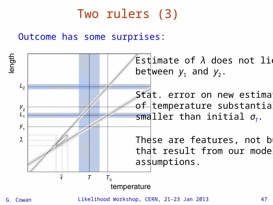
Outcome has some surprises:
Estimate of λ does not liebetween y1 and y2.
Stat. error on new estimateof temperature substantiallysmaller than initial σT.
These are features, not bugs,that result from our modelassumptions.
G. Cowan Likelihood Workshop, CERN, 21-23 Jan 2013 48
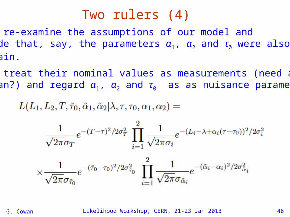
Two rulers (4)We may re-examine the assumptions of our model and conclude that, say, the parameters α1, α2 and τ0 were alsouncertain.
We may treat their nominal values as measurements (need a model;Gaussian?) and regard α1, α2 and τ0 as as nuisance parameters.
G. Cowan Likelihood Workshop, CERN, 21-23 Jan 2013 49
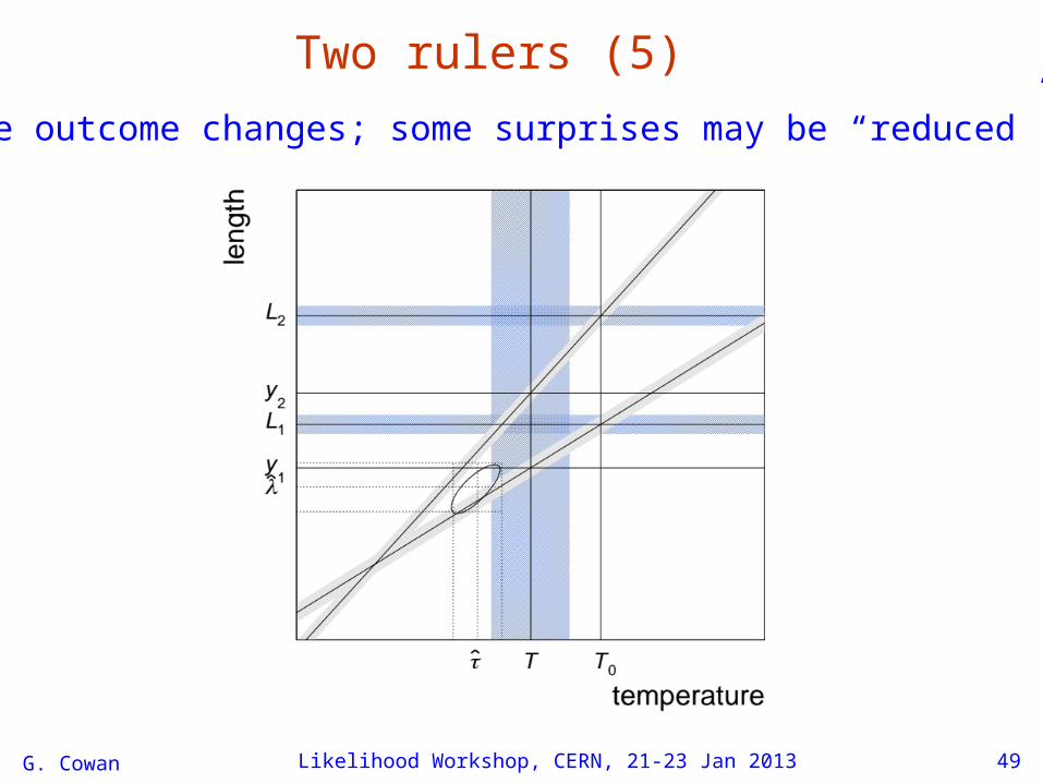
Two rulers (5)The outcome changes; some surprises may be “reduced”.
G. Cowan Likelihood Workshop, CERN, 21-23 Jan 2013 page 50
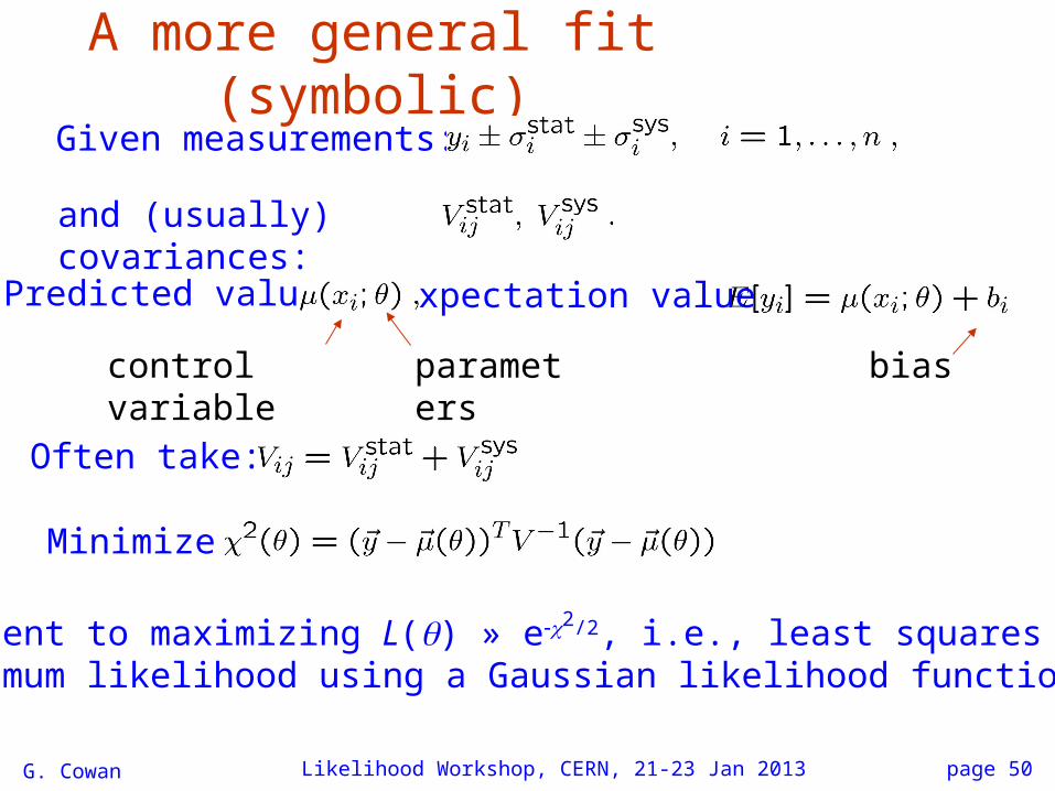
A more general fit (symbolic)Given measurements:
and (usually) covariances:
Predicted value:
control variable parameters bias
Often take:
Minimize
Equivalent to maximizing L() » eχ2/2, i.e., least squares same as maximum likelihood using a Gaussian likelihood function.
expectation value
G. Cowan Likelihood Workshop, CERN, 21-23 Jan 2013 page 51
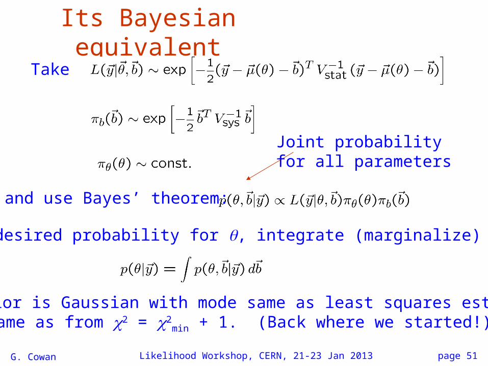
Its Bayesian equivalent
and use Bayes’ theorem:
To get desired probability for , integrate (marginalize) over b:
→ Posterior is Gaussian with mode same as least squares estimator, same as from χ2 = χ2
min + 1. (Back where we started!)
Take
Joint probabilityfor all parameters
G. Cowan Likelihood Workshop, CERN, 21-23 Jan 2013 page 52
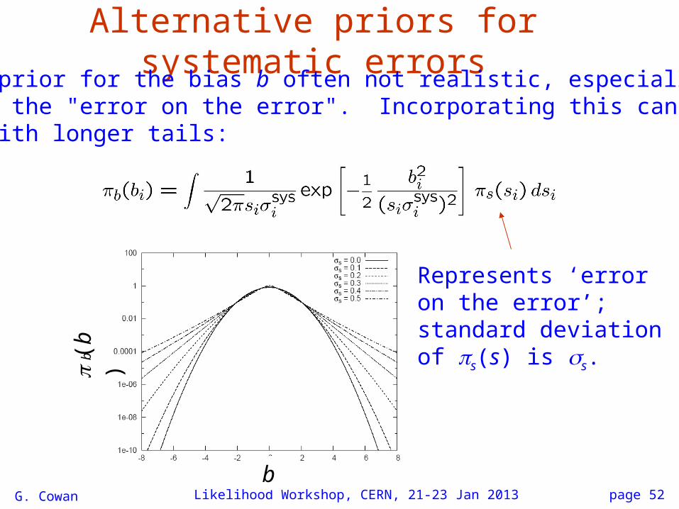
Alternative priors for systematic errorsGaussian prior for the bias b often not realistic, especially if oneconsiders the "error on the error". Incorporating this can givea prior with longer tails:
b(b
)
Represents ‘erroron the error’; standard deviation of s(s) is s.
b
G. Cowan Likelihood Workshop, CERN, 21-23 Jan 2013 page 53
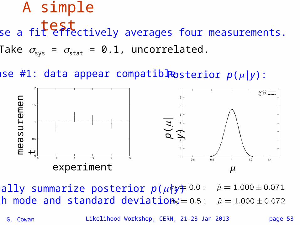
A simple testSuppose a fit effectively averages four measurements.
Take sys = stat = 0.1, uncorrelated.
Case #1: data appear compatible Posterior p(|y):
Usually summarize posterior p(|y) with mode and standard deviation:
experiment
mea
sure
me
nt
p(
|y)
G. Cowan Likelihood Workshop, CERN, 21-23 Jan 2013 page 54
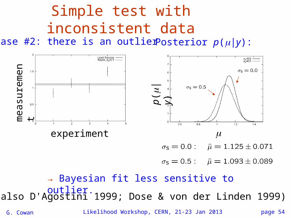
Simple test with inconsistent dataCase #2: there is an outlier
→ Bayesian fit less sensitive to outlier.
Posterior p(|y):
experiment
mea
sure
me
nt
p(|
y)
(See also D'Agostini 1999; Dose & von der Linden 1999)
G. Cowan Likelihood Workshop, CERN, 21-23 Jan 2013 55
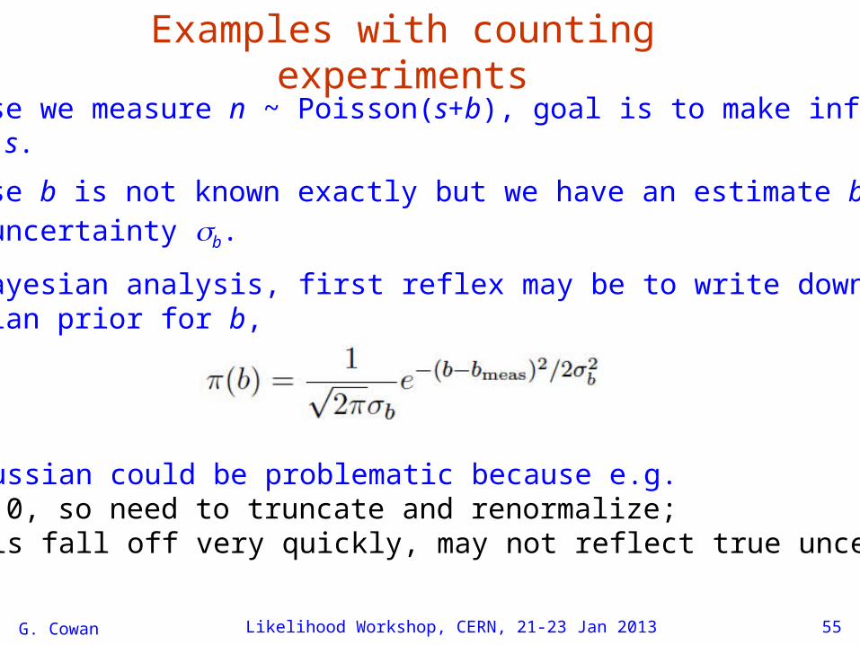
Examples with counting experimentsSuppose we measure n ~ Poisson(s+b), goal is to make inferenceabout s.
Suppose b is not known exactly but we have an estimate bmeas
with uncertainty b.
For Bayesian analysis, first reflex may be to write down a Gaussian prior for b,
But a Gaussian could be problematic because e.g.b ≥ 0, so need to truncate and renormalize;tails fall off very quickly, may not reflect true uncertainty.
G. Cowan Likelihood Workshop, CERN, 21-23 Jan 2013 56
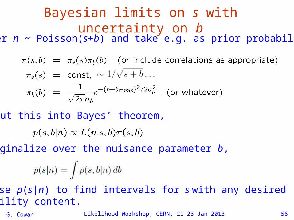
Bayesian limits on s with uncertainty on bConsider n ~ Poisson(s+b) and take e.g. as prior probabilities
Put this into Bayes’ theorem,
Marginalize over the nuisance parameter b,
Then use p(s|n) to find intervals for s with any desired probability content.
G. Cowan Likelihood Workshop, CERN, 21-23 Jan 2013 57
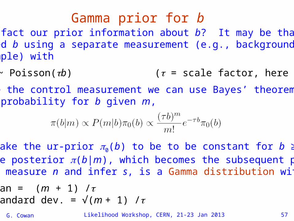
Gamma prior for bWhat is in fact our prior information about b? It may be that we estimated b using a separate measurement (e.g., background control sample) with
m ~ Poisson(b) ( = scale factor, here assume known)
Having made the control measurement we can use Bayes’ theoremto get the probability for b given m,
If we take the ur-prior 0(b) to be to be constant for b ≥ 0,then the posterior (b|m), which becomes the subsequent prior when we measure n and infer s, is a Gamma distribution with:
mean = (m + 1) /standard dev. = √(m + 1) /
G. Cowan Likelihood Workshop, CERN, 21-23 Jan 2013 58
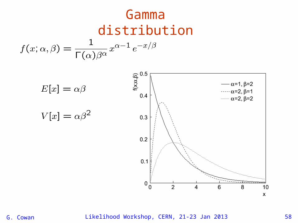
Gamma distribution
G. Cowan Likelihood Workshop, CERN, 21-23 Jan 2013 59
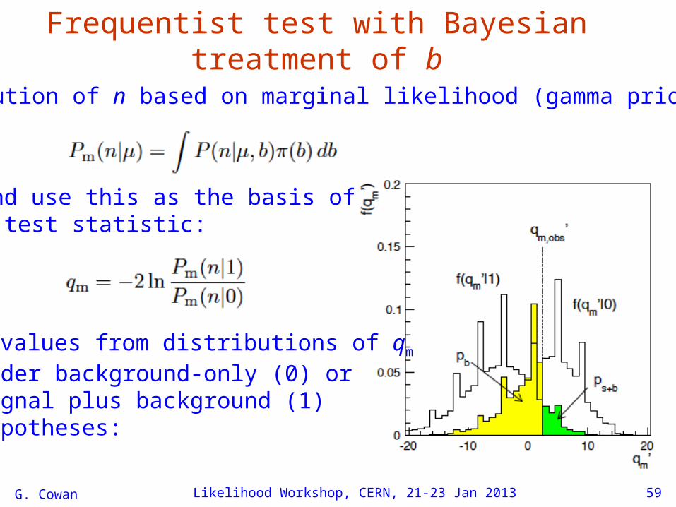
Frequentist test with Bayesian treatment of b
Distribution of n based on marginal likelihood (gamma prior for b):
and use this as the basis ofa test statistic:
p-values from distributions of qm
under background-only (0) or signal plus background (1) hypotheses:
G. Cowan Likelihood Workshop, CERN, 21-23 Jan 2013 60
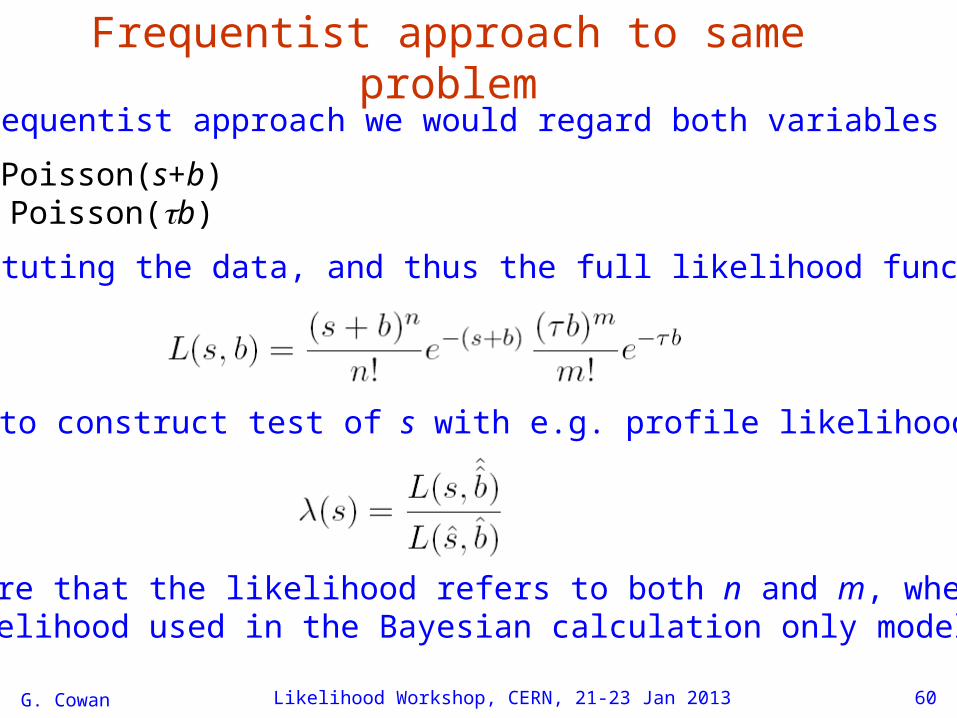
Frequentist approach to same problemIn the frequentist approach we would regard both variables
n ~ Poisson(s+b)m ~ Poisson(b)
as constituting the data, and thus the full likelihood function is
Use this to construct test of s with e.g. profile likelihood ratio
Note here that the likelihood refers to both n and m, whereasthe likelihood used in the Bayesian calculation only modeled n.
G. Cowan Likelihood Workshop, CERN, 21-23 Jan 2013 61
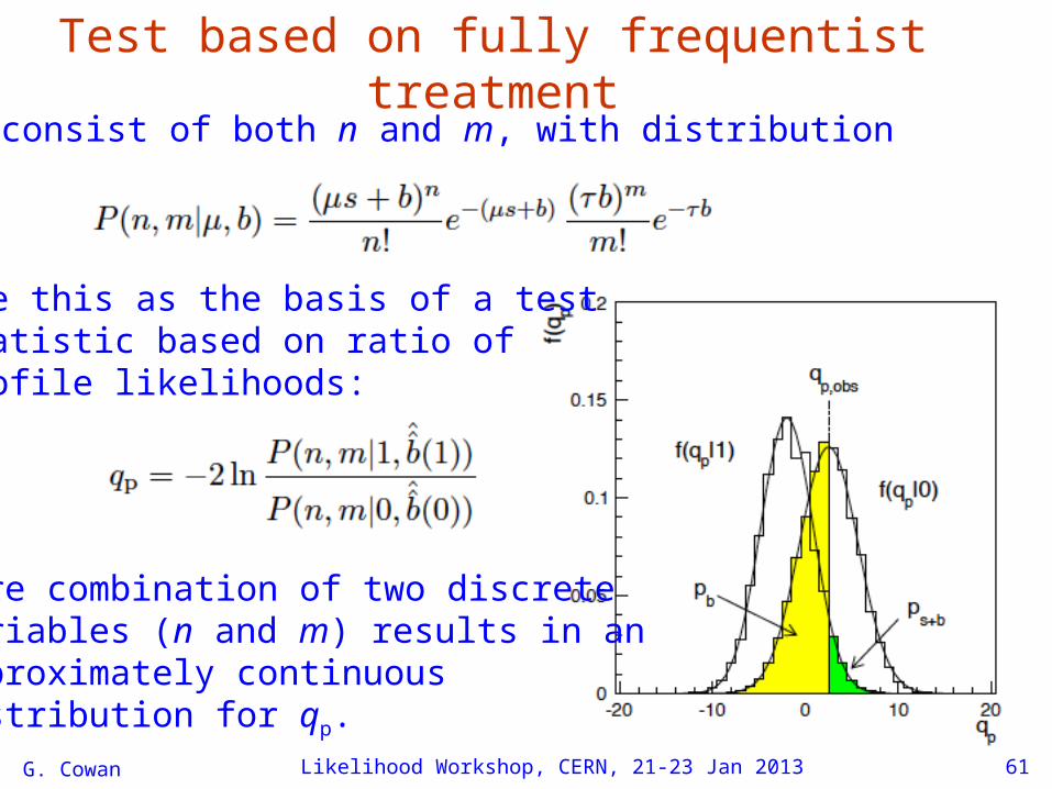
Test based on fully frequentist treatmentData consist of both n and m, with distribution
Use this as the basis of a teststatistic based on ratio of profile likelihoods:
Here combination of two discretevariables (n and m) results in anapproximately continuous distribution for qp.
G. Cowan Likelihood Workshop, CERN, 21-23 Jan 2013 62
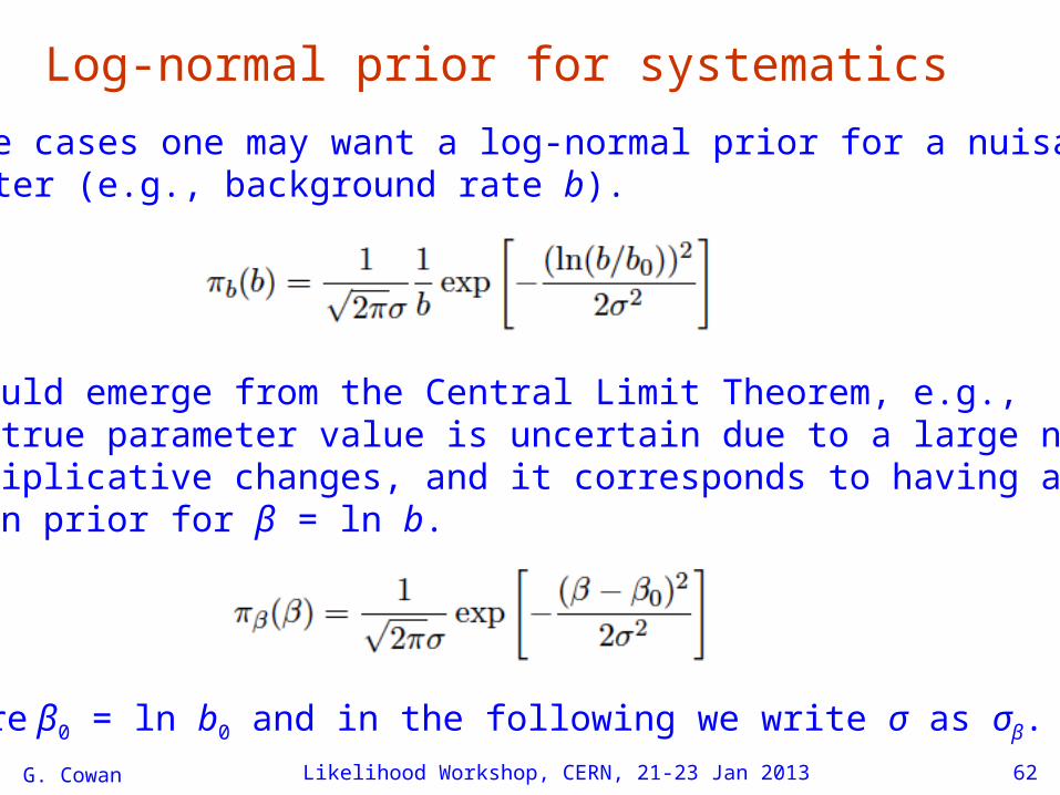
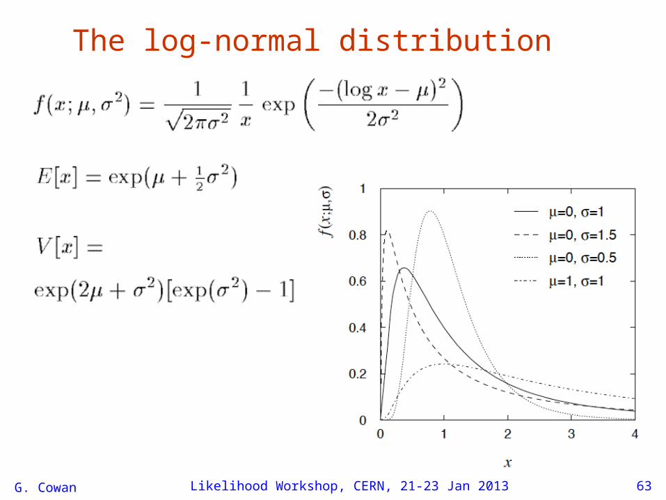
Log-normal prior for systematicsIn some cases one may want a log-normal prior for a nuisanceparameter (e.g., background rate b).
This would emerge from the Central Limit Theorem, e.g.,if the true parameter value is uncertain due to a large numberof multiplicative changes, and it corresponds to having aGaussian prior for β = ln b.
where β0 = ln b0 and in the following we write σ as σβ.
G. Cowan Likelihood Workshop, CERN, 21-23 Jan 2013 63
The log-normal distribution
G. Cowan Likelihood Workshop, CERN, 21-23 Jan 2013 64
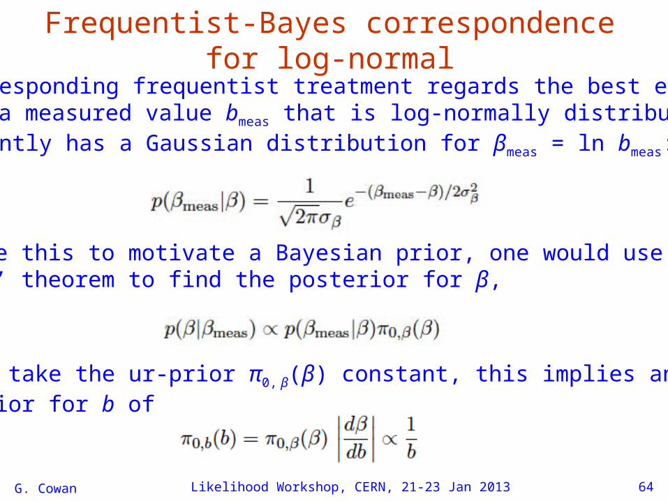
Frequentist-Bayes correspondence for log-normalThe corresponding frequentist treatment regards the best estimateof b as a measured value bmeas that is log-normally distributed, or equivalently has a Gaussian distribution for βmeas = ln bmeas:
To use this to motivate a Bayesian prior, one would useBayes’ theorem to find the posterior for β,
If we take the ur-prior π0, β(β) constant, this implies anur-prior for b of
G. Cowan Likelihood Workshop, CERN, 21-23 Jan 2013 65
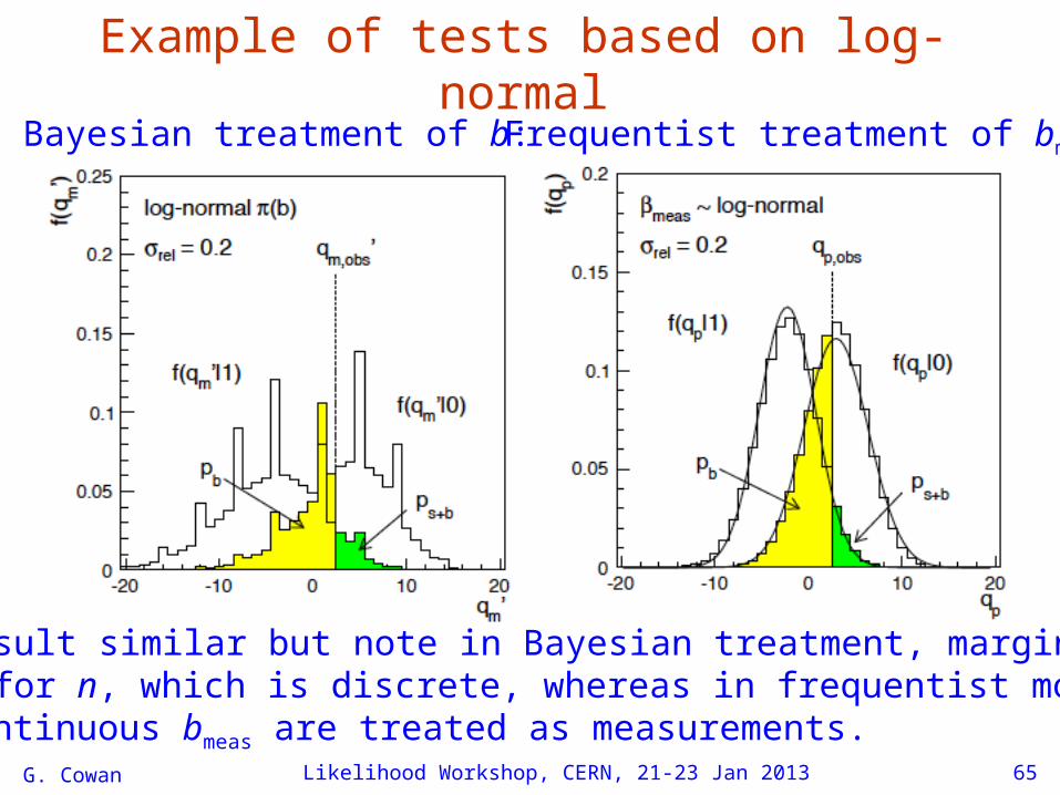
Example of tests based on log-normalBayesian treatment of b: Frequentist treatment of bmeas:
Final result similar but note in Bayesian treatment, marginal modelis only for n, which is discrete, whereas in frequentist model both n and continuous bmeas are treated as measurements.
G. Cowan Likelihood Workshop, CERN, 21-23 Jan 2013 66
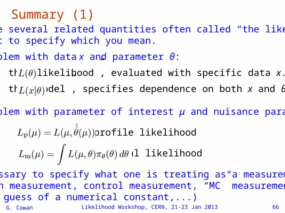
Summary (1)There are several related quantities often called “the likelihood”;important to specify which you mean.
In a problem with data x and parameter θ:
the “likelihood”, evaluated with specific data x.
the “model”, specifies dependence on both x and θ.
In a problem with parameter of interest μ and nuisance param. θ:
profile likelihood
marginal likelihood
Necessary to specify what one is treating as a measurement(main measurement, control measurement, “MC” measurement,best guess of a numerical constant,...)
G. Cowan Likelihood Workshop, CERN, 21-23 Jan 2013 67
Summary (2)Frequentist use of likelihoods (in general requires full model)
parameter estimation
tests, p-values
Operations involve maximization of L (minuit, etc.)
Bayesian use of likelihoods (requires only L for the real data)
Bayes’ theorem → posterior probability
marginalize over nuisance parameters
Operations involve integration (MCMC, nested sampling,...)
For both Bayesian and frequentist approaches, crucial point is tofind an accurate model, i.e., it must be “correct” for some point in its parameter space.

G. Cowan Likelihood Workshop, CERN, 21-23 Jan 2013 68
Extra slides
G. Cowan Likelihood Workshop, CERN, 21-23 Jan 2013 page 69
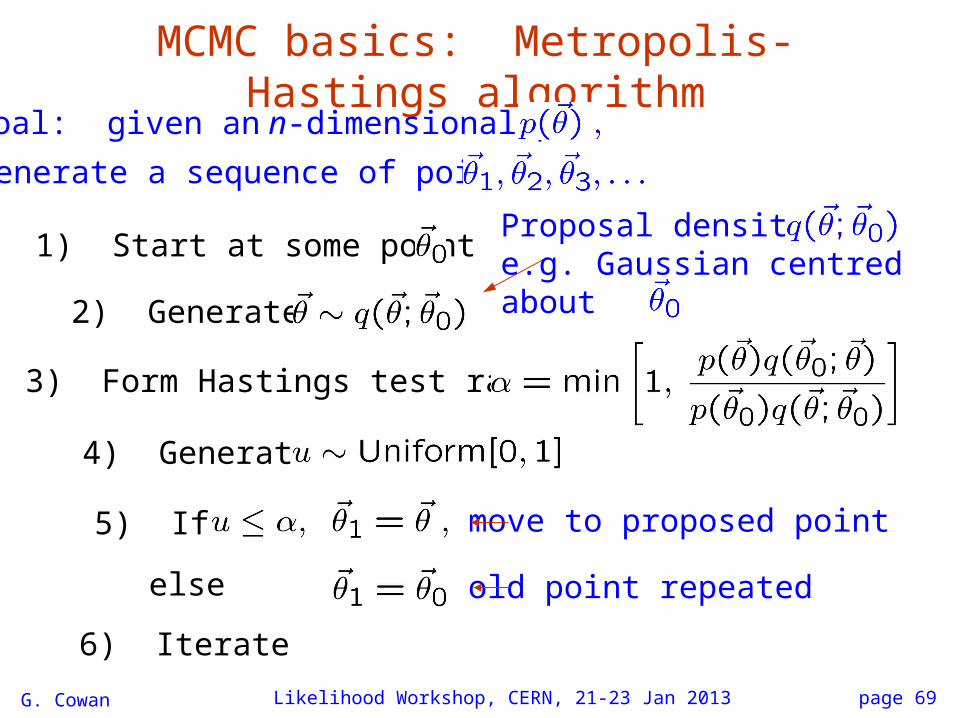
MCMC basics: Metropolis-Hastings algorithmGoal: given an n-dimensional pdf generate a sequence of points
1) Start at some point
2) Generate
Proposal densitye.g. Gaussian centredabout
3) Form Hastings test ratio
4) Generate
5) If
else
move to proposed point
old point repeated
6) Iterate
G. Cowan Likelihood Workshop, CERN, 21-23 Jan 2013 page 70
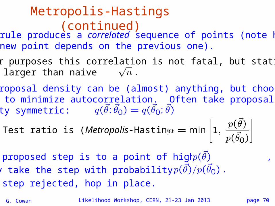
Metropolis-Hastings (continued)This rule produces a correlated sequence of points (note how each new point depends on the previous one).
For our purposes this correlation is not fatal, but statisticalerrors larger than naive
The proposal density can be (almost) anything, but chooseso as to minimize autocorrelation. Often take proposaldensity symmetric:
Test ratio is (Metropolis-Hastings):
I.e. if the proposed step is to a point of higher , take it; if not, only take the step with probability If proposed step rejected, hop in place.

G. Cowan Likelihood Workshop, CERN, 21-23 Jan 2013 page 71
Metropolis-Hastings caveatsActually one can only prove that the sequence of points followsthe desired pdf in the limit where it runs forever.
There may be a “burn-in” period where the sequence doesnot initially follow
Unfortunately there are few useful theorems to tell us when thesequence has converged.
Look at trace plots, autocorrelation.
Check result with different proposal density.
If you think it’s converged, try starting from a differentpoint and see if the result is similar.
G. Cowan Likelihood Workshop, CERN, 21-23 Jan 2013 page 72
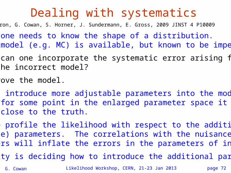
Dealing with systematics
Suppose one needs to know the shape of a distribution.Initial model (e.g. MC) is available, but known to be imperfect.
Q: How can one incorporate the systematic error arising fromuse of the incorrect model?
A: Improve the model.
That is, introduce more adjustable parameters into the modelso that for some point in the enlarged parameter space it is very close to the truth.
Then use profile the likelihood with respect to the additional(nuisance) parameters. The correlations with the nuisance parameters will inflate the errors in the parameters of interest.
Difficulty is deciding how to introduce the additional parameters.
S. Caron, G. Cowan, S. Horner, J. Sundermann, E. Gross, 2009 JINST 4 P10009
page 73
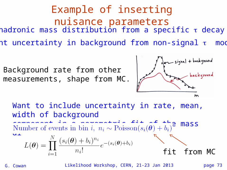
Example of inserting nuisance parameters
G. Cowan Likelihood Workshop, CERN, 21-23 Jan 2013
Fit of hadronic mass distribution from a specific decay mode.
Important uncertainty in background from non-signal modes.
Background rate from other measurements, shape from MC.
Want to include uncertainty in rate, mean, width of backgroundcomponent in a parametric fit of the mass distribution.
fit from MC
page 74
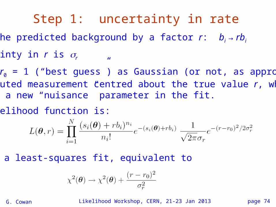
Step 1: uncertainty in rate
G. Cowan Likelihood Workshop, CERN, 21-23 Jan 2013
Scale the predicted background by a factor r: bi → rbi
Uncertainty in r is r
Regard r0 = 1 (“best guess”) as Gaussian (or not, as appropriate)distributed measurement centred about the true value r, which becomes a new “nuisance” parameter in the fit.
New likelihood function is:
For a least-squares fit, equivalent to
page 75
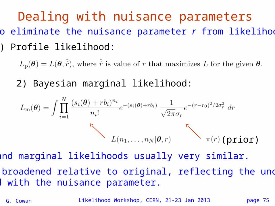
Dealing with nuisance parameters
G. Cowan Likelihood Workshop, CERN, 21-23 Jan 2013
Ways to eliminate the nuisance parameter r from likelihood.
1) Profile likelihood:
2) Bayesian marginal likelihood:
(prior)
Profile and marginal likelihoods usually very similar.
Both are broadened relative to original, reflecting the uncertainty connected with the nuisance parameter.
page 76
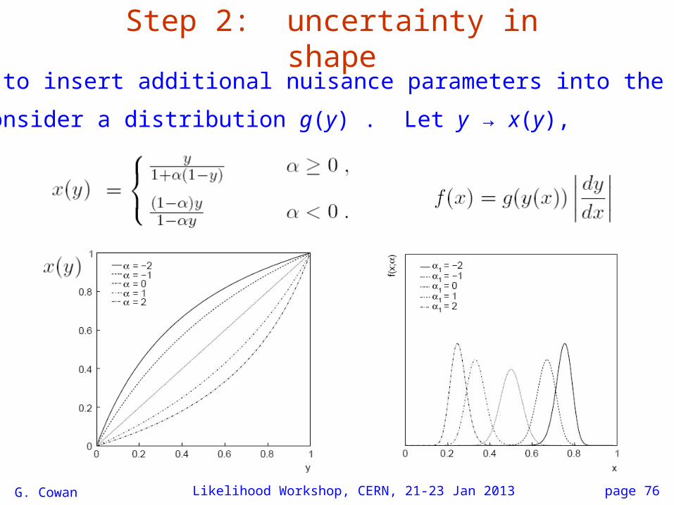
Step 2: uncertainty in shape
G. Cowan Likelihood Workshop, CERN, 21-23 Jan 2013
Key is to insert additional nuisance parameters into the model.
E.g. consider a distribution g(y) . Let y → x(y),
page 77
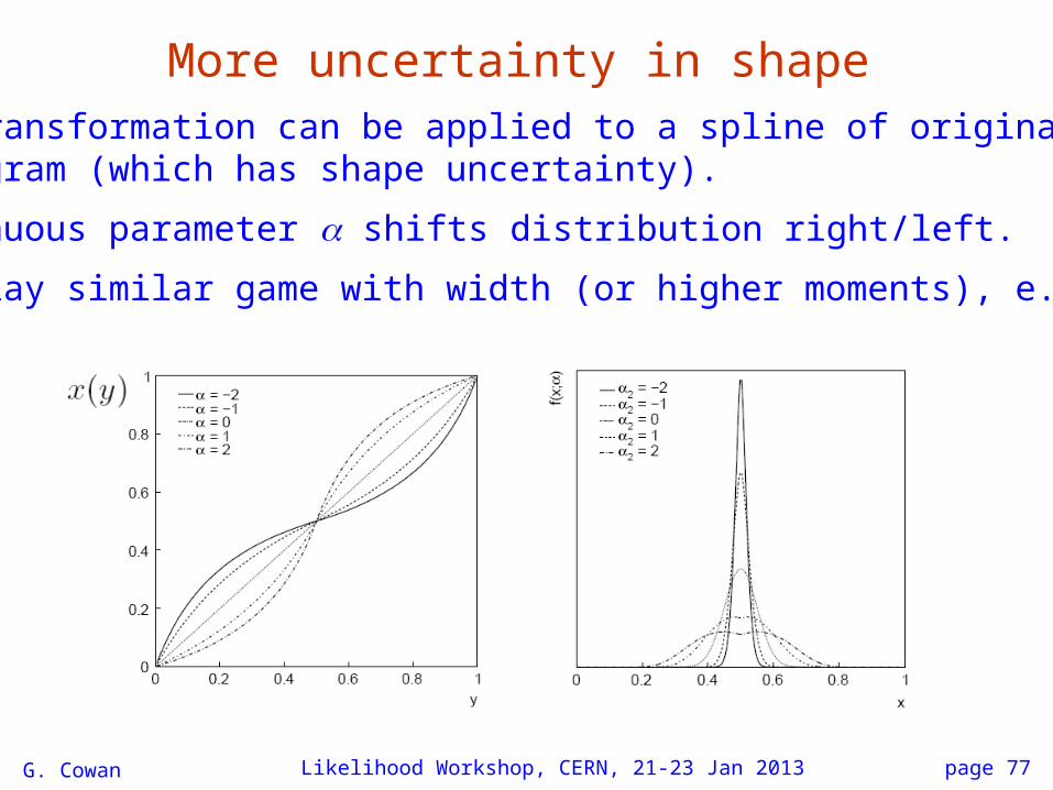
More uncertainty in shape
G. Cowan Likelihood Workshop, CERN, 21-23 Jan 2013
The transformation can be applied to a spline of original MChistogram (which has shape uncertainty).
Continuous parameter shifts distribution right/left.
Can play similar game with width (or higher moments), e.g.,
page 78
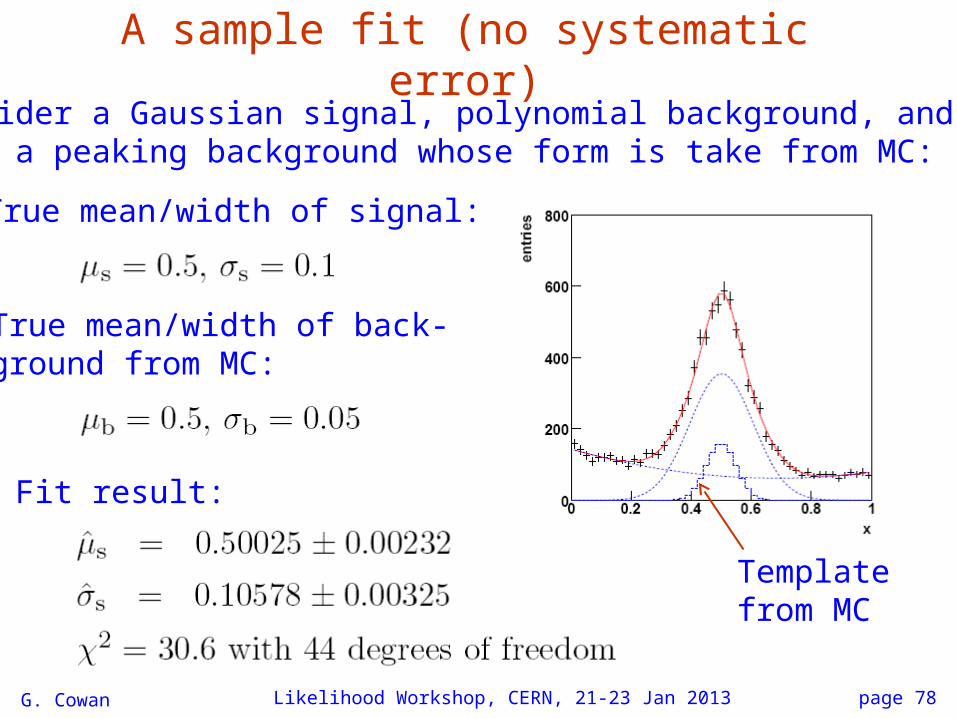
A sample fit (no systematic error)
G. Cowan Likelihood Workshop, CERN, 21-23 Jan 2013
Consider a Gaussian signal, polynomial background, andalso a peaking background whose form is take from MC:
Template from MC
True mean/width of signal:
True mean/width of back-ground from MC:
Fit result:
page 79
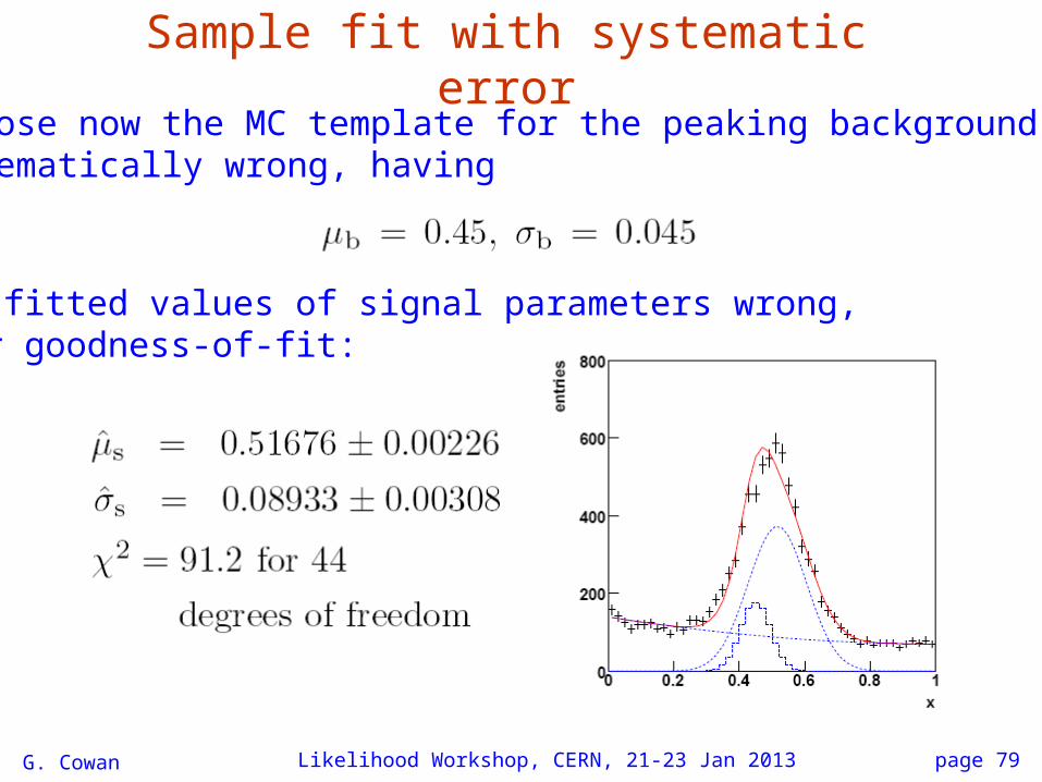
Sample fit with systematic error
G. Cowan Likelihood Workshop, CERN, 21-23 Jan 2013
Suppose now the MC template for the peaking background wassystematically wrong, having
Now fitted values of signal parameters wrong, poor goodness-of-fit:
page 80
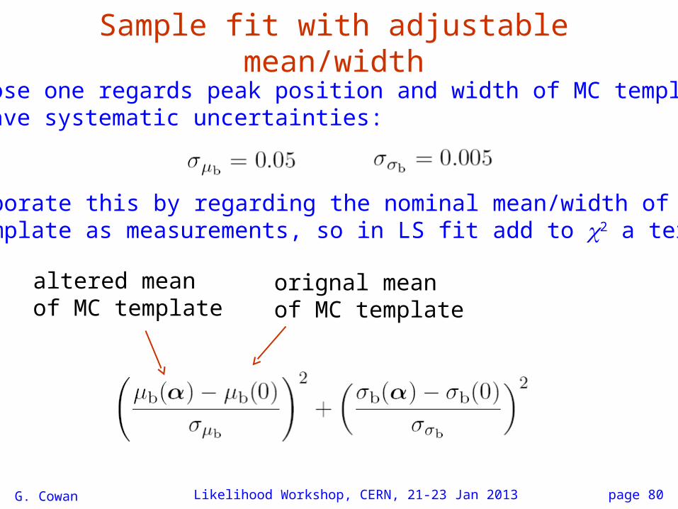
Sample fit with adjustable mean/width
G. Cowan Likelihood Workshop, CERN, 21-23 Jan 2013
Suppose one regards peak position and width of MC templateto have systematic uncertainties:
Incorporate this by regarding the nominal mean/width of theMC template as measurements, so in LS fit add to χ2 a term:
orignal mean of MC template
altered mean of MC template
page 81
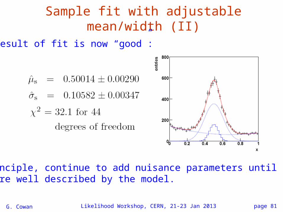
Sample fit with adjustable mean/width (II)
G. Cowan Likelihood Workshop, CERN, 21-23 Jan 2013
Result of fit is now “good”:
In principle, continue to add nuisance parameters until data are well described by the model.
page 82
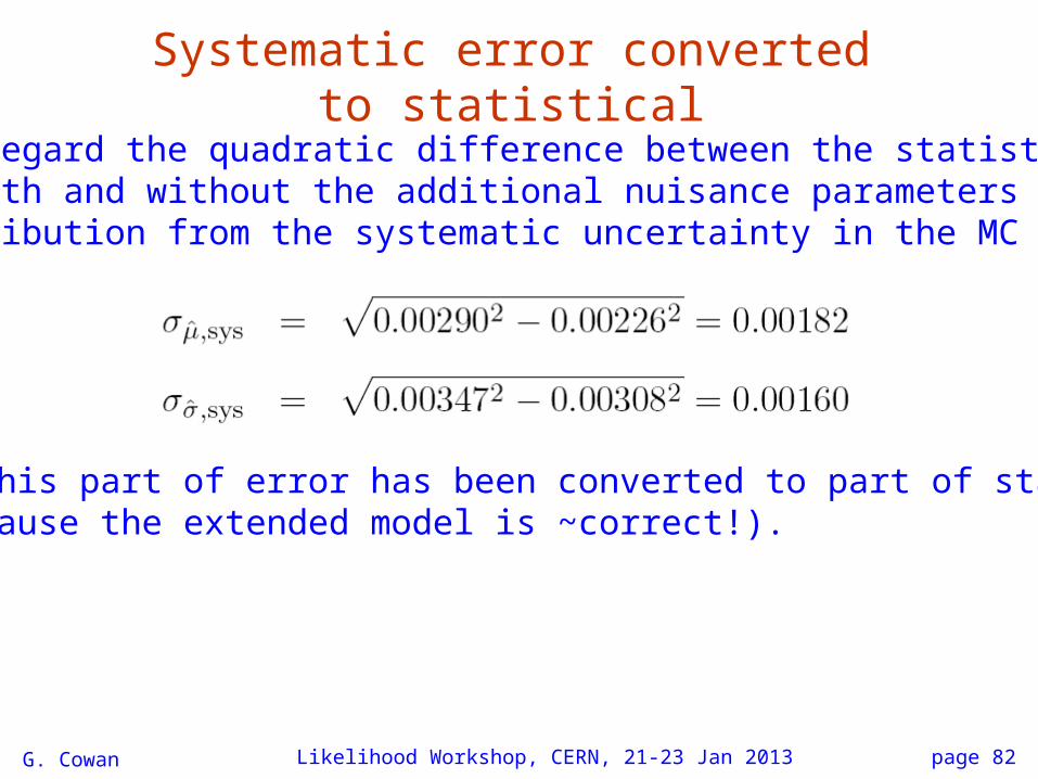
Systematic error converted to statistical
G. Cowan Likelihood Workshop, CERN, 21-23 Jan 2013
One can regard the quadratic difference between the statisticalerrors with and without the additional nuisance parameters asthe contribution from the systematic uncertainty in the MC template:
Formally this part of error has been converted to part of statisticalerror (because the extended model is ~correct!).
page 83
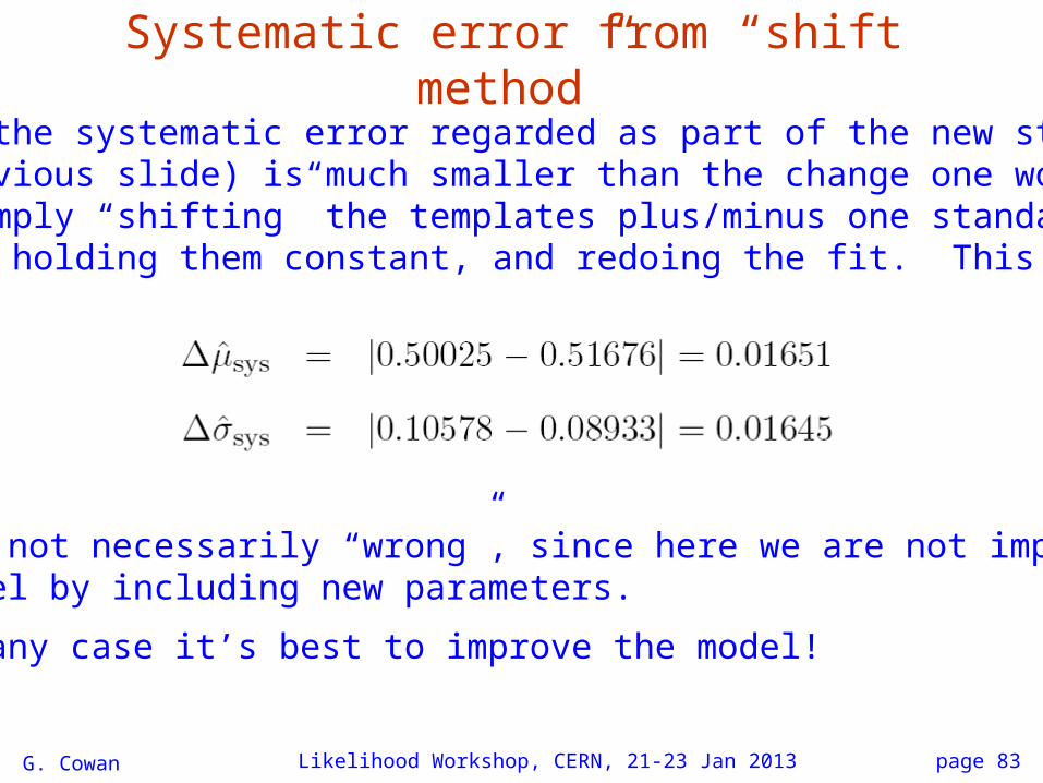
Systematic error from “shift method”
G. Cowan Likelihood Workshop, CERN, 21-23 Jan 2013
Note that the systematic error regarded as part of the new statistical error (previous slide) is much smaller than the change one would find by simply “shifting” the templates plus/minus one standard deviation, holding them constant, and redoing the fit. This gives:
This is not necessarily “wrong”, since here we are not improvingthe model by including new parameters.
But in any case it’s best to improve the model!
G. Cowan Likelihood Workshop, CERN, 21-23 Jan 2013 page 84
Issues with finding an improved modelSometimes, e.g., if the data set is very large, the total χ2 canbe very high (bad), even though the absolute deviation betweenmodel and data may be small.
It may be that including additional parameters "spoils" theparameter of interest and/or leads to an unphysical fit resultwell before it succeeds in improving the overall goodness-of-fit.
Include new parameters in a clever (physically motivated,local) way, so that it affects only the required regions.
Use Bayesian approach -- assign priors to the new nuisanceparameters that constrain them from moving too far (or use equivalent frequentist penalty terms in likelihood).
Unfortunately these solutions may not be practical and one maybe forced to use ad hoc recipes (last resort).
G. Cowan Likelihood Workshop, CERN, 21-23 Jan 2013 85
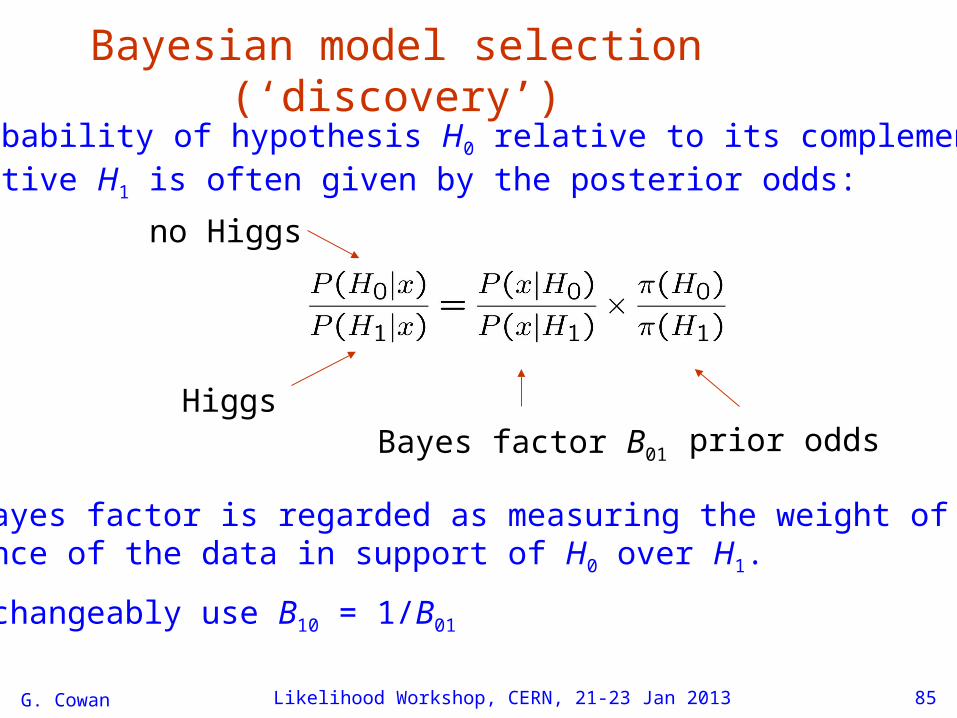
Bayesian model selection (‘discovery’)
no Higgs
Higgs
The probability of hypothesis H0 relative to its complementaryalternative H1 is often given by the posterior odds:
Bayes factor B01 prior odds
The Bayes factor is regarded as measuring the weight of evidence of the data in support of H0 over H1.
Interchangeably use B10 = 1/B01
G. Cowan Likelihood Workshop, CERN, 21-23 Jan 2013 86
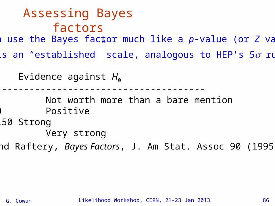
Assessing Bayes factorsOne can use the Bayes factor much like a p-value (or Z value).
There is an “established” scale, analogous to HEP's 5 rule:
B10 Evidence against H0
--------------------------------------------1 to 3 Not worth more than a bare mention3 to 20 Positive20 to 150 Strong> 150 Very strong
Kass and Raftery, Bayes Factors, J. Am Stat. Assoc 90 (1995) 773.
G. Cowan Likelihood Workshop, CERN, 21-23 Jan 2013 87
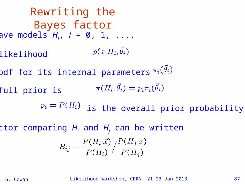
Rewriting the Bayes factorSuppose we have models Hi, i = 0, 1, ...,
each with a likelihood
and a prior pdf for its internal parameters
so that the full prior is
where is the overall prior probability for Hi.
The Bayes factor comparing Hi and Hj can be written
G. Cowan Likelihood Workshop, CERN, 21-23 Jan 2013 88
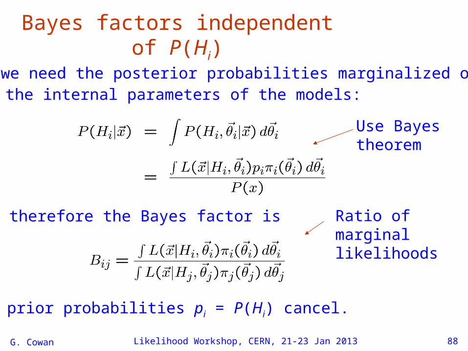
Bayes factors independent of P(Hi)
For Bij we need the posterior probabilities marginalized overall of the internal parameters of the models:
Use Bayestheorem
So therefore the Bayes factor is
The prior probabilities pi = P(Hi) cancel.
Ratio of marginal likelihoods
G. Cowan Likelihood Workshop, CERN, 21-23 Jan 2013 89
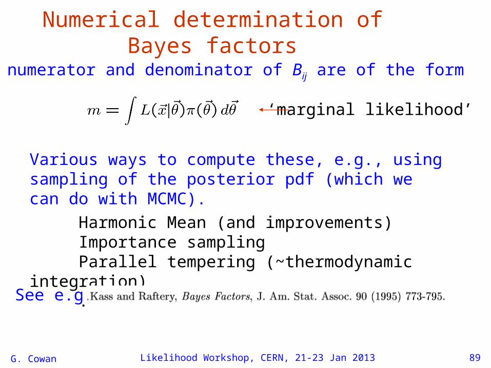
Numerical determination of Bayes factors
Both numerator and denominator of Bij are of the form
‘marginal likelihood’
Various ways to compute these, e.g., using sampling of the posterior pdf (which we can do with MCMC).
Harmonic Mean (and improvements)Importance samplingParallel tempering (~thermodynamic integration)...
See e.g.
G. Cowan Likelihood Workshop, CERN, 21-23 Jan 2013 90
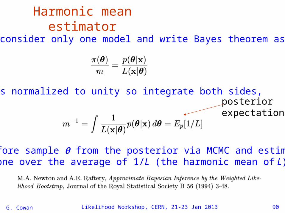
Harmonic mean estimatorE.g., consider only one model and write Bayes theorem as:
() is normalized to unity so integrate both sides,
Therefore sample from the posterior via MCMC and estimate m with one over the average of 1/L (the harmonic mean of L).
posteriorexpectation
G. Cowan Likelihood Workshop, CERN, 21-23 Jan 2013 91
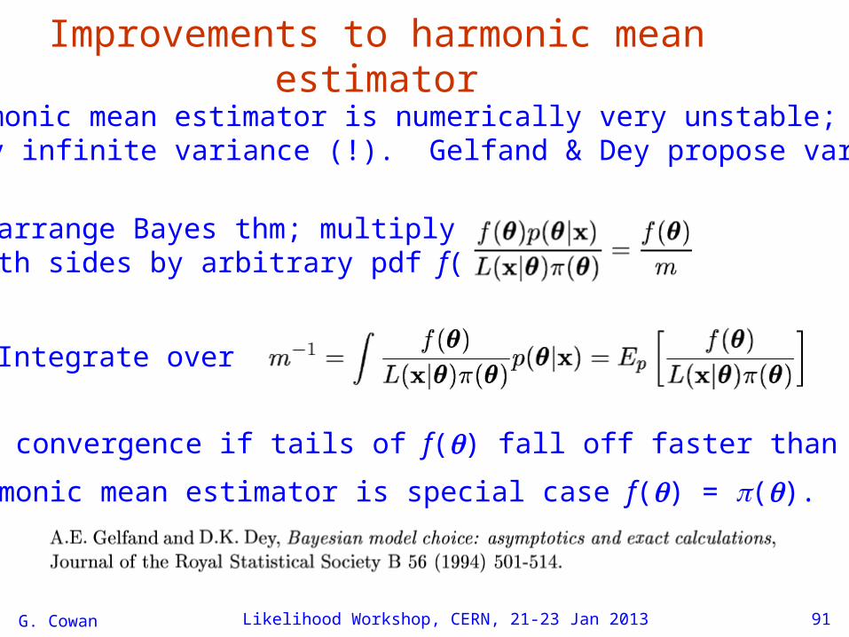
Improvements to harmonic mean estimatorThe harmonic mean estimator is numerically very unstable;formally infinite variance (!). Gelfand & Dey propose variant:
Rearrange Bayes thm; multiply both sides by arbitrary pdf f():
Integrate over :
Improved convergence if tails of f() fall off faster than L(x|)()
Note harmonic mean estimator is special case f() = ()..
G. Cowan Likelihood Workshop, CERN, 21-23 Jan 2013 92
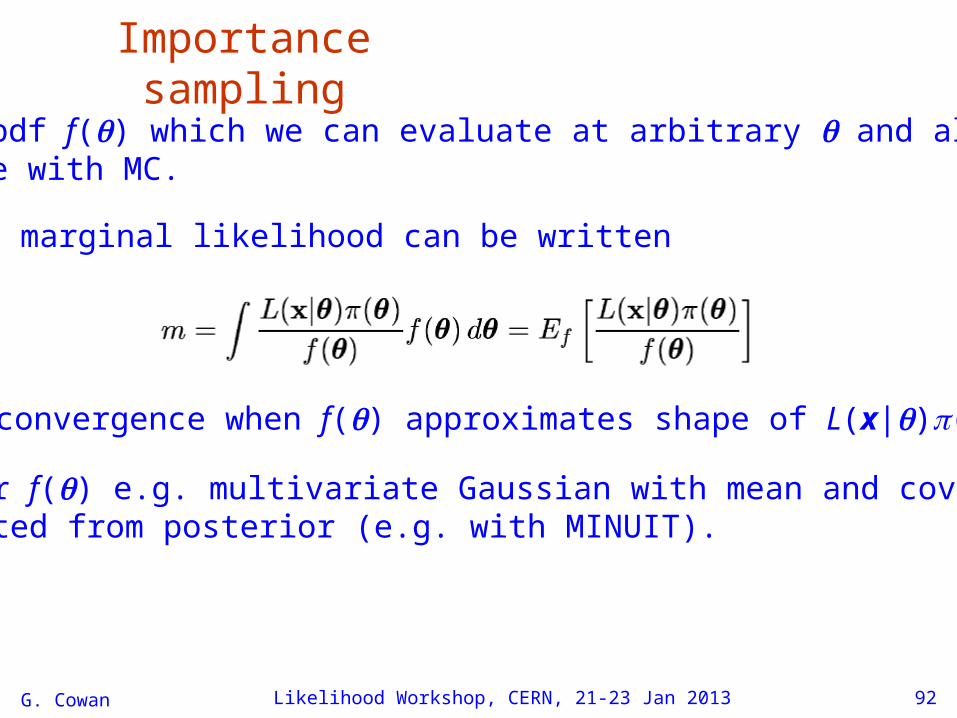
Importance samplingNeed pdf f() which we can evaluate at arbitrary and alsosample with MC.
The marginal likelihood can be written
Best convergence when f() approximates shape of L(x|)().
Use for f() e.g. multivariate Gaussian with mean and covarianceestimated from posterior (e.g. with MINUIT).
G. Cowan Likelihood Workshop, CERN, 21-23 Jan 2013 93
Bayes factor computation discussionAlso tried method of parallel tempering; see note on course web page and also
Harmonic mean OK for very rough estimate.
I had trouble with all of the methods based on posterior sampling.
Importance sampling worked best, but may not scale well to higher dimensions.
Lots of discussion of this problem in the literature, e.g.,
94G. Cowan
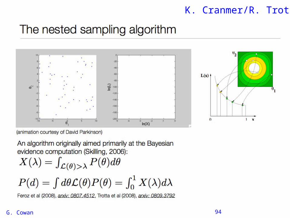
K. Cranmer/R. Trotta