Using Propensity Score Analysis to Assess Effectiveness of Social Marketing Campaigns in Healthcare: An Example

from Medicare Open EnrollmentFrank Funderburk, Diane Field,

& Clarese AstrinDivision of Research

Office of Communications Centers for Medicare and Medicaid Services

The statements expressed here are those of the authors and do not necessarily reflect the views or policies of CMS

Assessing Medicare Open Enrollment (OE)

• Annual pre-post survey to assess beneficiary awareness of benefits and behavior during OE

• Domains covered –– Awareness– Knowledge– Review/Compare Rate– Satisfaction with plan

• But -- Was campaign effective?

Traditional Approaches

• Pre vs. Post• Cross-Tabs• Regression

adjustments for covariates

• Sub-group comparisons

Pearson chi2(1) = 11.2442 Pr = 0.001

100.00 100.00 100.00 38.97 61.03 100.00 Total 403 631 1,034 30.27 40.57 36.56 32.28 67.72 100.00 1 122 256 378 69.73 59.43 63.44 42.84 57.16 100.00 0 281 375 656 ADEXPOSE 0 1 Total REVIEW

column percentage row percentage frequency Key

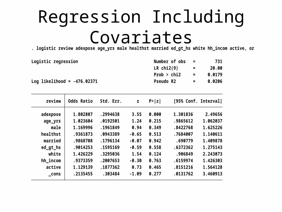
Regression Including Covariates

_cons .2135455 .303484 -1.09 0.277 .0131762 3.460913 active 1.129139 .1877362 0.73 0.465 .8151216 1.564128 hh_incom .9373359 .2007653 -0.30 0.763 .6159974 1.426303 white 1.426229 .3295036 1.54 0.124 .906849 2.243073 ed_gt_hs .9014253 .1595169 -0.59 0.558 .6372362 1.275143 married .9868708 .1796134 -0.07 0.942 .690779 1.409878 healthst .9361873 .0943389 -0.65 0.513 .7684007 1.140611 male 1.169996 .1961849 0.94 0.349 .8422768 1.625226 age_yrs 1.023604 .0192501 1.24 0.215 .9865612 1.062037 adexpose 1.802807 .2994638 3.55 0.000 1.301836 2.49656 review Odds Ratio Std. Err. z P>|z| [95% Conf. Interval]

Log likelihood = -476.02371 Pseudo R2 = 0.0206 Prob > chi2 = 0.0179 LR chi2(9) = 20.00Logistic regression Number of obs = 731

. logistic review adexpose age_yrs male healthst married ed_gt_hs white hh_incom active, or

Limitations• Treatment is not randomly assigned, so other

variables (other than seeing the Medicare TV ad) may contribute to the beneficiaries decision to review coverage options.

• Self-selection or other nonrandom selection processes can be mistaken for treatment effects.

• Missing data on one or more covariates can also be a source of bias.

Propensity Scores• Propensity score matching aims to “correct” the estimation

of treatment effects in observational studies. Apples to apples comparisons.

• Identify treated and untreated subjects who are as identical as possible on key covariates

• Summarize characteristics of subjects into a single variable to facilitate matching

• Allow one to mimic counterfactual substitutes and make causal inferences (under certain conditions)

• Illustrate approach with data from Medicare OE, with focus on exposure to TV advertising and reviewing coverage options during OE

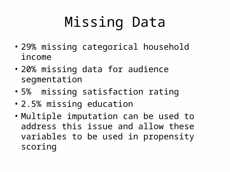
Missing Data

• 29% missing categorical household income• 20% missing data for audience segmentation• 5% missing satisfaction rating• 2.5% missing education• Multiple imputation can be used to address

this issue and allow these variables to be used in propensity scoring

How It’s Done

• Forget about your outcome variable(s)• Model treatment exposure (saw Medicare TV ad)

with logistic regression – use potential predictors of treatment exposure EXCEPT those that are outcomes of treatment exposure

• Estimate predicted value of exposure from model• Use propensity score in analysis to estimate

treatment effect

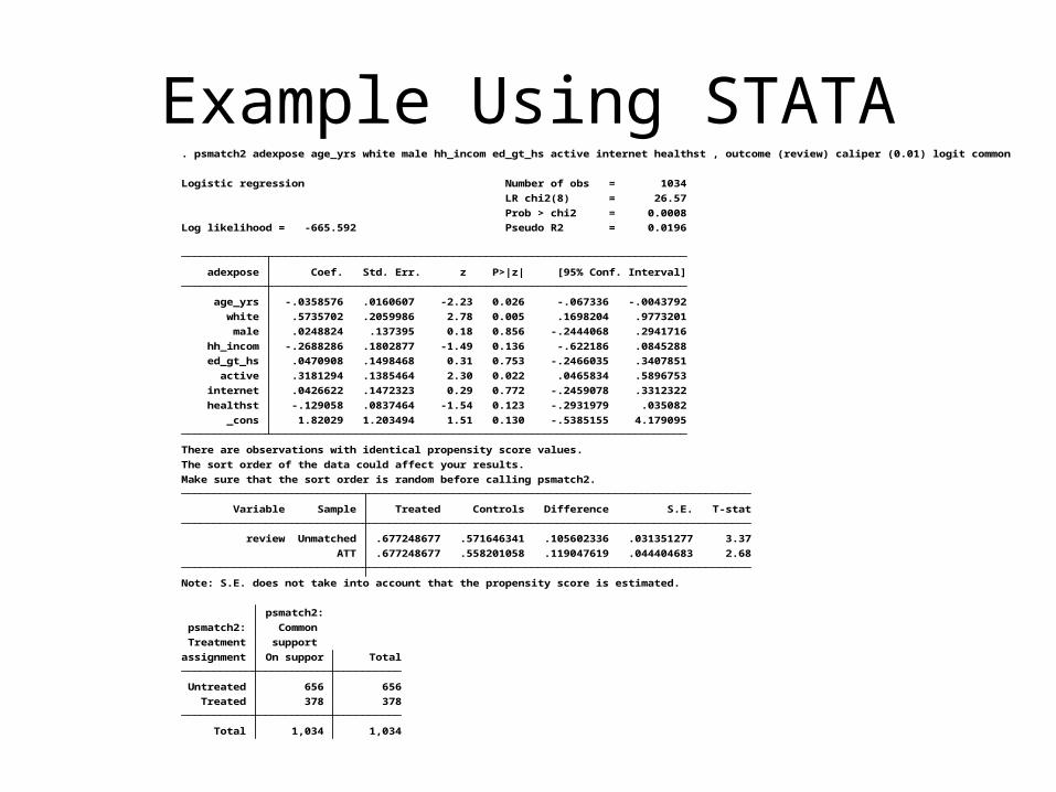
Example Using STATA

Total 1,034 1,034

Treated 378 378

Untreated 656 656

assignment On suppor Total

Treatment support

psmatch2: Common

psmatch2:

Note: S.E. does not take into account that the propensity score is estimated.

ATT .677248677 .558201058 .119047619 .044404683 2.68

review Unmatched .677248677 .571646341 .105602336 .031351277 3.37

Variable Sample Treated Controls Difference S.E. T-stat

Make sure that the sort order is random before calling psmatch2.

The sort order of the data could affect your results.

There are observations with identical propensity score values.

_cons 1.82029 1.203494 1.51 0.130 -.5385155 4.179095

healthst -.129058 .0837464 -1.54 0.123 -.2931979 .035082

internet .0426622 .1472323 0.29 0.772 -.2459078 .3312322

active .3181294 .1385464 2.30 0.022 .0465834 .5896753

ed_gt_hs .0470908 .1498468 0.31 0.753 -.2466035 .3407851

hh_incom -.2688286 .1802877 -1.49 0.136 -.622186 .0845288

male .0248824 .137395 0.18 0.856 -.2444068 .2941716

white .5735702 .2059986 2.78 0.005 .1698204 .9773201

age_yrs -.0358576 .0160607 -2.23 0.026 -.067336 -.0043792

adexpose Coef. Std. Err. z P>|z| [95% Conf. Interval]

Log likelihood = -665.592 Pseudo R2 = 0.0196

Prob > chi2 = 0.0008

LR chi2(8) = 26.57

Logistic regression Number of obs = 1034

. psmatch2 adexpose age_yrs white male hh_incom ed_gt_hs active internet healthst , outcome (review) caliper (0.01) logit common

Compute Propensity Scores

• Propensity score is defined as the probability of being treated given a subject’s background characteristics (i.e., conditional probability).

• Goal is balance in confounders between treated and untreated groups

1159. 125 0 .29005229 0 0 1158. 124 0 .2697903 1 1 1157. 123 0 .29468183 1 1 1156. 122 0 .3317468 1 1 1155. 121 0 .38531767 1 1 1154. 120 1 .28771362 1 1 1153. 119 0 .33151058 1 1 1152. 118 0 .43305978 1 1 1151. 117 0 .26540466 1 1 1150. 116 0 .38454591 1 1 1149. 115 0 .42859445 1 1 1148. 114 0 .25304612 0 0 1147. 113 1 .35822347 1 1 1146. 112 1 .35281371 1 1 1145. 111 0 .3168519 0 0 1144. 110 1 .28953402 1 1 1143. 109 1 .40309792 1 1 1142. 108 0 .33928792 1 1 1141. 107 0 .32403488 0 0 1140. 106 1 .33003463 1 1 1139. 105 0 .29112737 1 1 1138. 104 0 .45973876 1 1 1137. 103 0 .32770283 1 1 1136. 102 0 .30655524 1 1 1135. 101 0 .45578216 1 1 CaseID adexpose _pscore review review

. list CaseID adexpose _pscore review review in 1135/1160, table

Balance and Bias Reduction

Matched 2.9558 2.9712 -1.9 71.4 -0.25 0.800 healthst Unmatched 2.9558 3.0099 -6.5 -1.02 0.309 Matched .46561 .46032 1.1 89.0 0.15 0.884 internet Unmatched .46561 .41768 9.7 1.50 0.135 Matched .38889 .3836 1.1 93.3 0.15 0.881 active Unmatched .38889 .30945 16.7 2.61 0.009 Matched .18519 .20106 -3.9 72.2 -0.55 0.581 hh_incom Unmatched .18519 .24238 -14.0 -2.14 0.033 Matched .64021 .63492 1.1 85.5 0.15 0.880 ed_gt_hs Unmatched .64021 .60366 7.5 1.16 0.245 Matched .43122 .4418 -2.1 11.9 -0.29 0.770 male Unmatched .43122 .41921 2.4 0.38 0.707 Matched .90212 .90476 -0.8 95.7 -0.12 0.902 white Unmatched .90212 .83994 18.6 2.81 0.005 Matched 72.148 71.963 4.4 74.1 0.62 0.535 age_yrs Unmatched 72.148 72.864 -17.1 -2.64 0.008 Variable Sample Treated Control %bias |bias| t p>|t| Mean %reduct t-test

. pstest age_yrs white male ed_gt_hs hh_incom active internet healthst

Diagnosing Matching

.1 .2 .3 .4 .5 .6Propensity Score

Untreated Treated

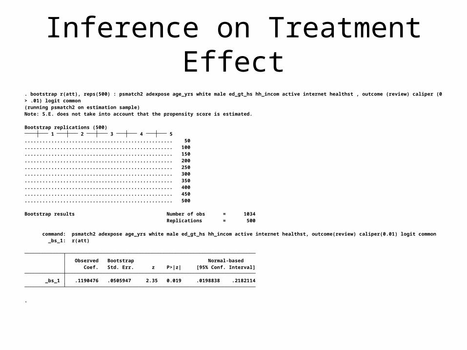
Inference on Treatment Effect

.

_bs_1 .1190476 .0505947 2.35 0.019 .0198838 .2182114 Coef. Std. Err. z P>|z| [95% Conf. Interval] Observed Bootstrap Normal-based

_bs_1: r(att) command: psmatch2 adexpose age_yrs white male ed_gt_hs hh_incom active internet healthst, outcome(review) caliper(0.01) logit common

Replications = 500Bootstrap results Number of obs = 1034

.................................................. 500

.................................................. 450

.................................................. 400

.................................................. 350

.................................................. 300

.................................................. 250

.................................................. 200

.................................................. 150

.................................................. 100

.................................................. 50 1 2 3 4 5 Bootstrap replications (500)

Note: S.E. does not take into account that the propensity score is estimated.(running psmatch2 on estimation sample)> .01) logit common. bootstrap r(att), reps(500) : psmatch2 adexpose age_yrs white male ed_gt_hs hh_incom active internet healthst , outcome (review) caliper (0

Modeling Other Effects

Propensity Score Analysis Issues

• Model specification• Matching approach• Effect estimates• Control for unobserved variables [absence of]• Missing values for covariates• Trade offs of precision and bias related to

“support”• Others

Some Benefits

• Increases attention on need to evaluate degree of overlap/balance between conditions

• Helps one think about design of observational studies

• Clear diagnostics• Reduces confounding• Complements rather than replaces other

analytic tools

Contact Information

Frank FunderburkDirector, Division of ResearchOffice of CommunicationsCenters for Medicare and Medicaid Servicesfrank.funderburk@cms.hhs.gov(410)786-1820