Embed Size (px)
Citation preview

Fundamentals to Biostatistics
Prof. Chandan ChakrabortyAssociate Professor
School of Medical Science & TechnologyIIT Kharagpur

Statistics
Math. StatisticsApplied Statistics
Biostatistics
collection, analysis, interpretation of data
development of new statistical theory & inference
application of the methods derived from math. statistics to subject specific areas like psychology, economics and public health
statistical methods are applied to medical, health and biological data
Areas of application of Biostatistics: Environmental Health, Genetics, Pharmaceutical research, Nutrition, Epidemiology and Health surveys etc
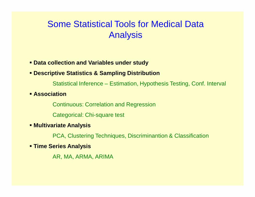
Some Statistical Tools for Medical Data Analysis
Data collection and Variables under study
Descriptive Statistics & Sampling Distribution
Statistical Inference – Estimation, Hypothesis Testing, Conf. Interval
Association
Continuous: Correlation and Regression
Categorical: Chi-square test
Multivariate Analysis
PCA, Clustering Techniques, Discriminantion & Classification
Time Series Analysis
AR, MA, ARMA, ARIMA

Population vs. SampleParameter vs. Statistics

Variable
Definition: characteristic of interest in a study that has different values for different individuals.
Two types of variableContinuous: values form continuumDiscrete: assume discrete set of values
ExamplesContinuous: blood pressure
Discrete: case/control, drug/placebo

6
Univariate Data• Measurements on a single variable X• Consider a continuous (numerical) variable• Summarizing X
– Numerically• Center• Spread
– Graphically• Boxplot• Histogram

7
Measures of center: Mean
• The mean value of a variable is obtained by computing the total of the values divided by the number of values
• Appropriate for distributions that are fairly symmetrical
• It is sensitive to presence of outliers, since all values contribute equally

8
Measures of center: Median• The median value of a variable is the number
having 50% (half) of the values smaller than it (and the other half bigger)
• It is NOT sensitive to presence of outliers, since it ‘ignores’ almost all of the data values
• The median is thus usually a more appropriate summary for skewed distributions
9
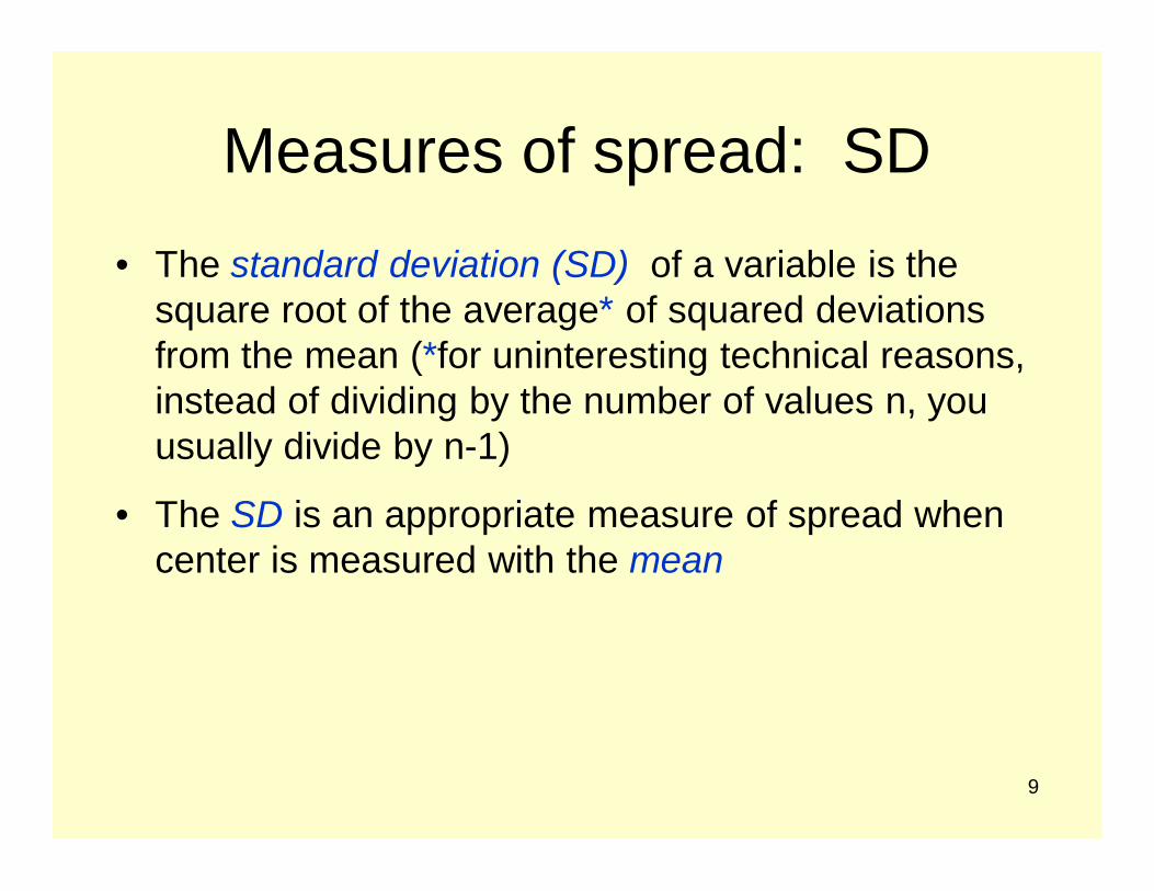
Measures of spread: SD• The standard deviation (SD) of a variable is the
square root of the average* of squared deviations from the mean (*for uninteresting technical reasons, instead of dividing by the number of values n, you usually divide by n-1)
• The SD is an appropriate measure of spread when center is measured with the mean
10
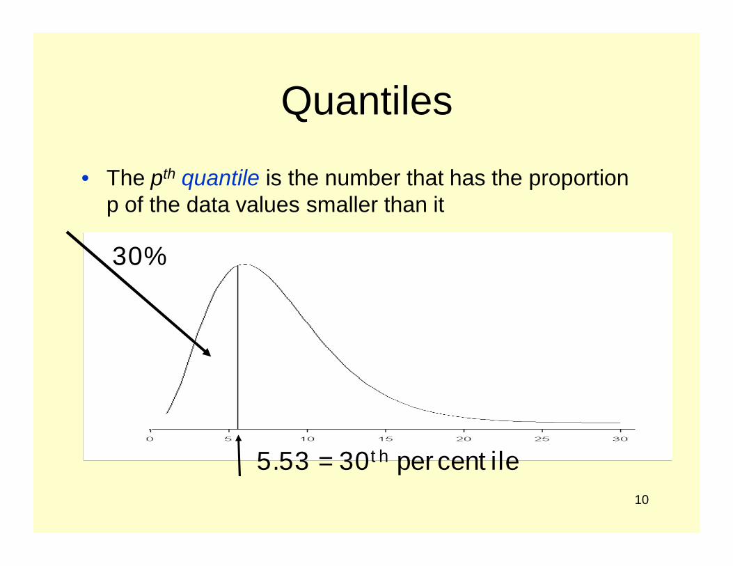
Quantiles
• The pth quantile is the number that has the proportion p of the data values smaller than it
30%
5.53 = 30th percentile
11
Measures of spread: IQR• The 25th (Q1), 50th (median), and 75th (Q3)
percentiles divide the data into 4 equal parts; these special percentiles are called quartiles
• The interquartile range (IQR) of a variable is the distance between Q1 and Q3:
IQR = Q3 – Q1
• The IQR is one way to measure spread when center is measured with the median
12
Five-number summary and boxplot
• An overall summary of the distribution of variable values is given by the five values:
Min, Q1, Median, Q3, and Max
• A boxplot provides a visual summary of this five-number summary
• Display boxplots side-by-side to compare distributions of different data sets

13
Boxplot
median
Q3
Q1
suspected outliers
`whiskers
14
Histogram
• A histogram is a special kind of bar plot
• It allows you to visualize the distribution of values for a numerical variable
• When drawn with a density scale:– the AREA (NOT height) of each bar is the proportion of
observations in the interval
– the TOTAL AREA is 100% (or 1)

15
Bivariate Data
• Bivariate data are just what they sound like – data with measurements on twovariables; let’s call them X and Y
• Here, we are looking at two continuousvariables
• Want to explore the relationship between the two variables

16
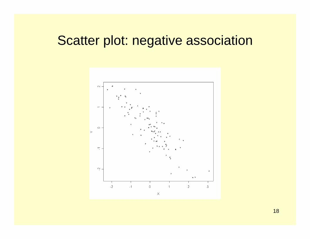
Scatter plot• We can graphically summarize a bivariate data set
with a scatter plot (also sometimes called a scatter diagram)
• Plots values of one variable on the horizontal axis and values of the other on the vertical axis
• Can be used to see how values of 2 variables tend to move with each other (i.e. how the variables are associated)

17
Scatter plot: positive association
18
Scatter plot: negative association

19
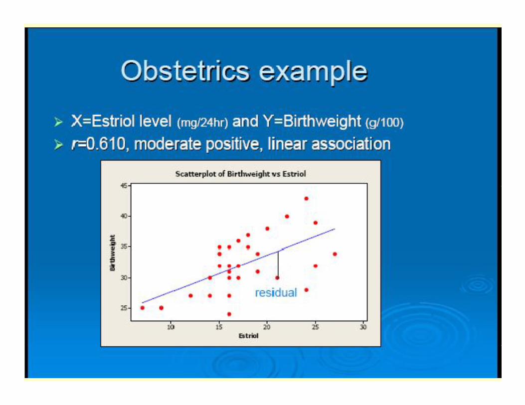
Scatter plot: real data example

20
Correlation Coefficient
• r is a unitless quantity• -1 r 1• r is a measure of LINEAR ASSOCIATION• When r = 0, the points are not LINEARLYASSOCIATED – this does NOT mean there is NO ASSOCIATION

Breast cancer example
Study on whether age at first child birth is an important risk factor for breast cancer (BC)
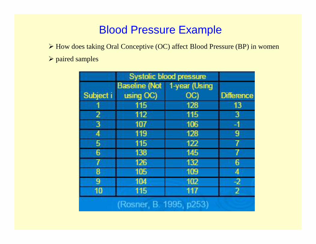
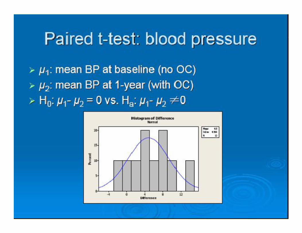
How does taking Oral Conceptive (OC) affect Blood Pressure (BP) in women
paired samples
Blood Pressure Example

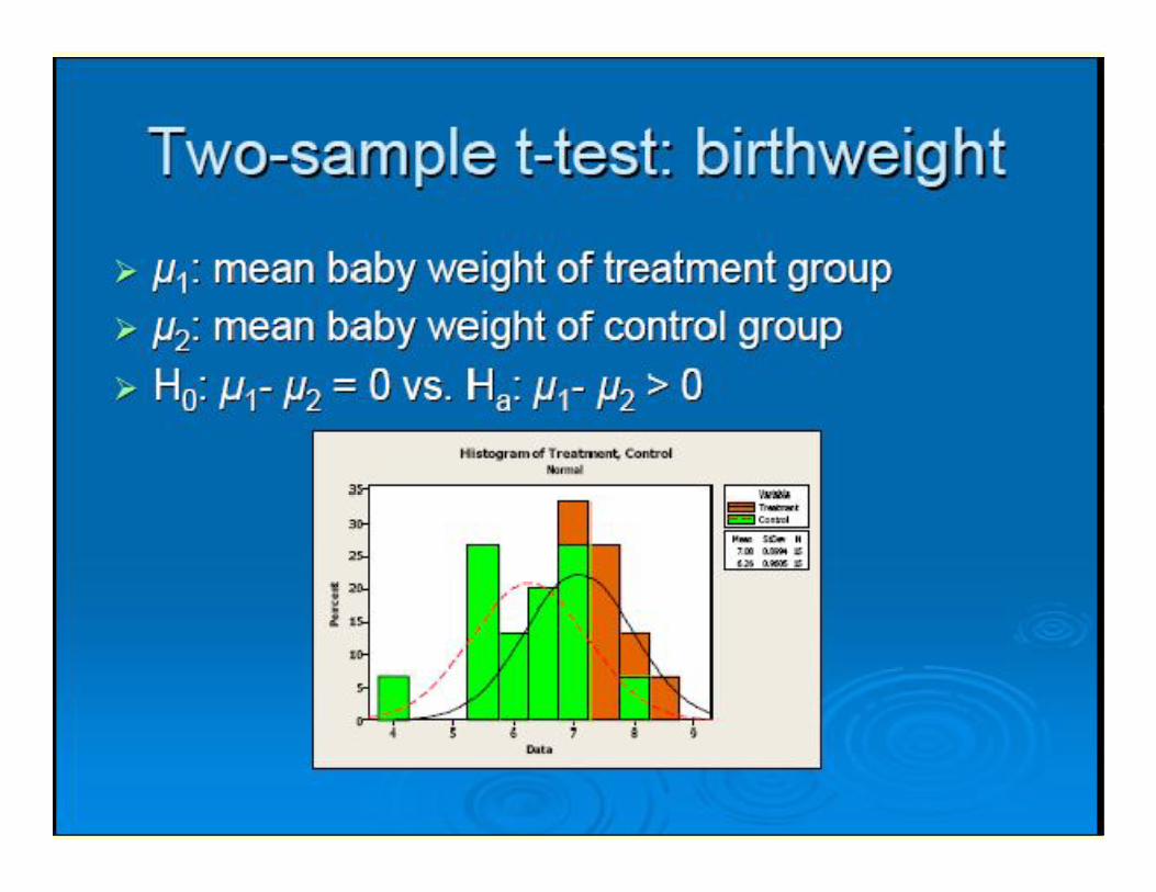
Birthweight Example
Determine the effectiveness of drugA on preventing premature birth.
Independent samples.


ParameterParameterStatisticStatistic
Mean:
Standard deviation:
Proportion:
s
X ____
____
____
estimates
estimates
estimates
from sample from entire population
p
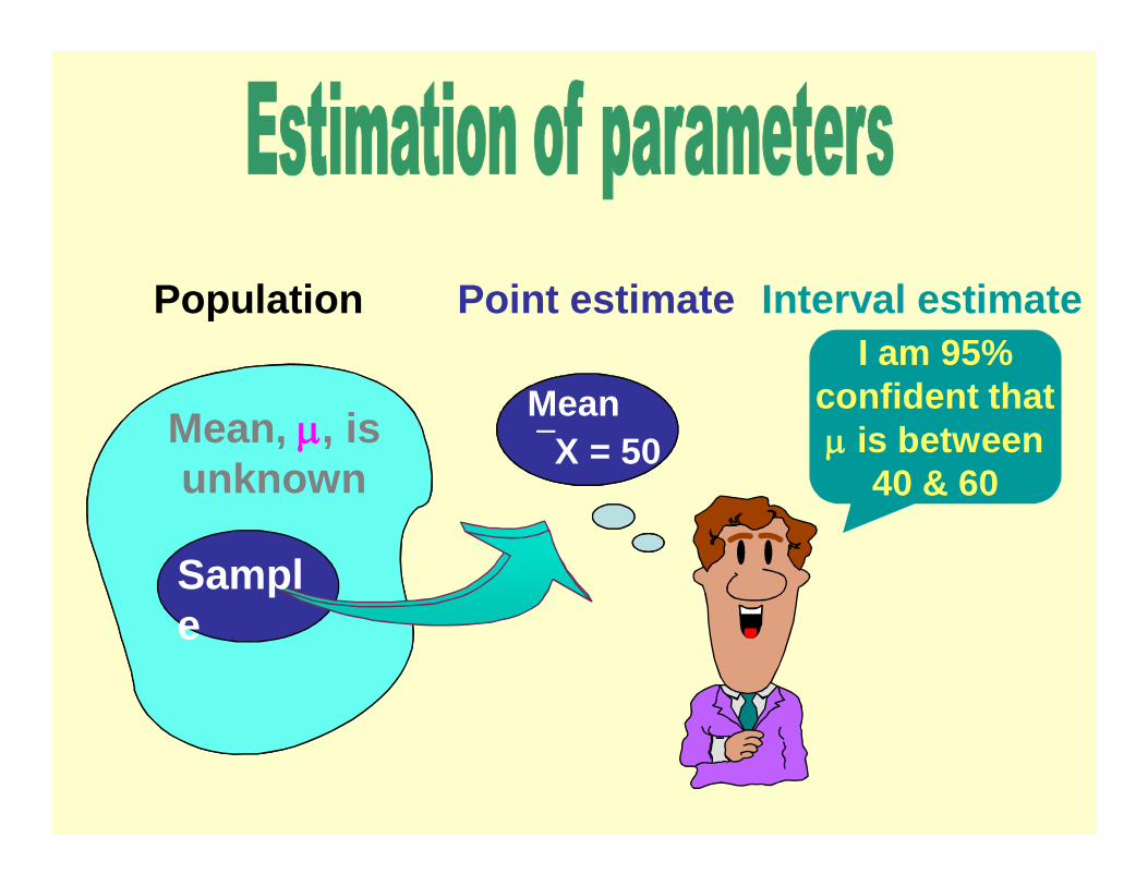
Mean, , is unknown
Population Point estimateI am 95%
confident that is between
40 & 60
Mean X = 50
Sample
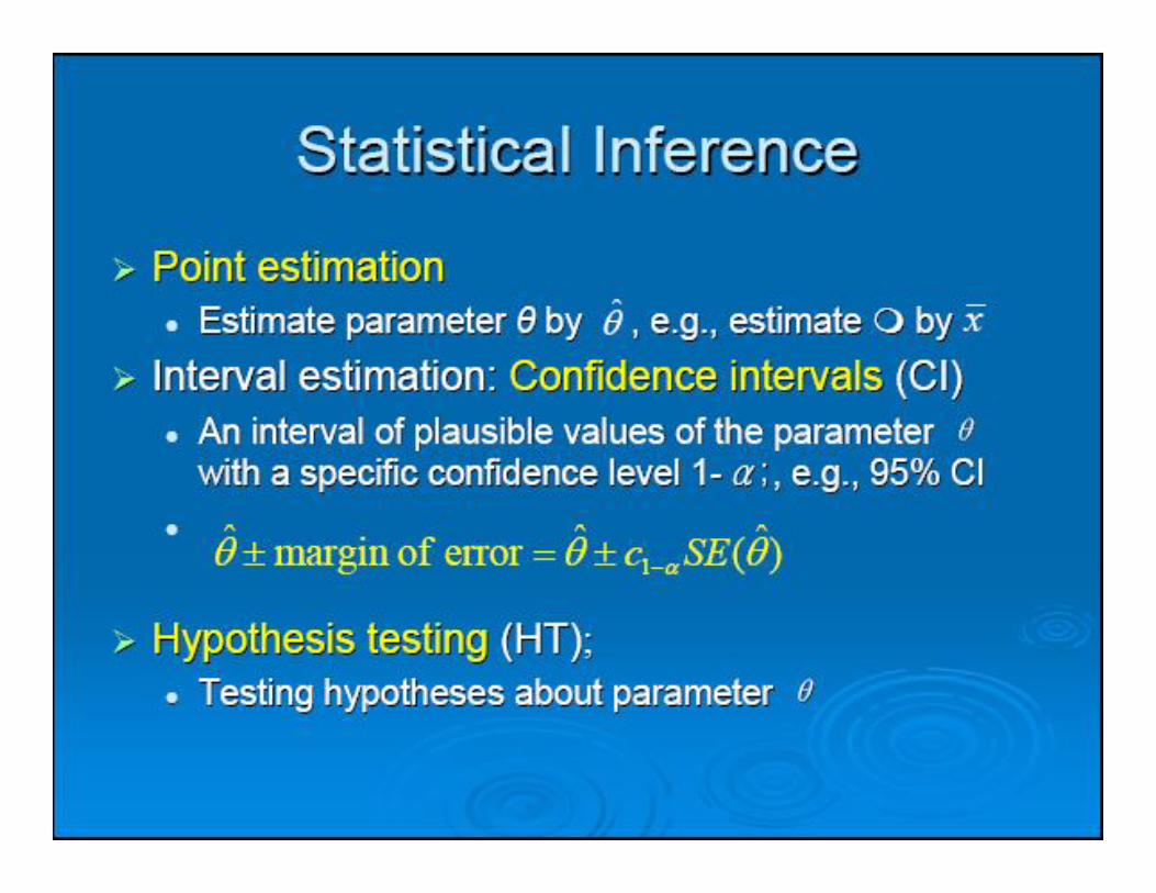
Interval estimate

Parameter
= Statistic ± Its Error

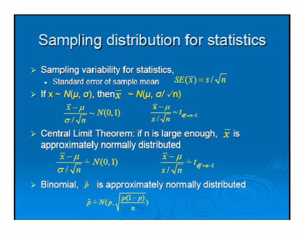
Sampling Distribution
X or PX or P X or P

Standard Error
SE (Mean) = S
n
SE (p) =
p(1-p)
n
Quantitative Variable
Qualitative Variable
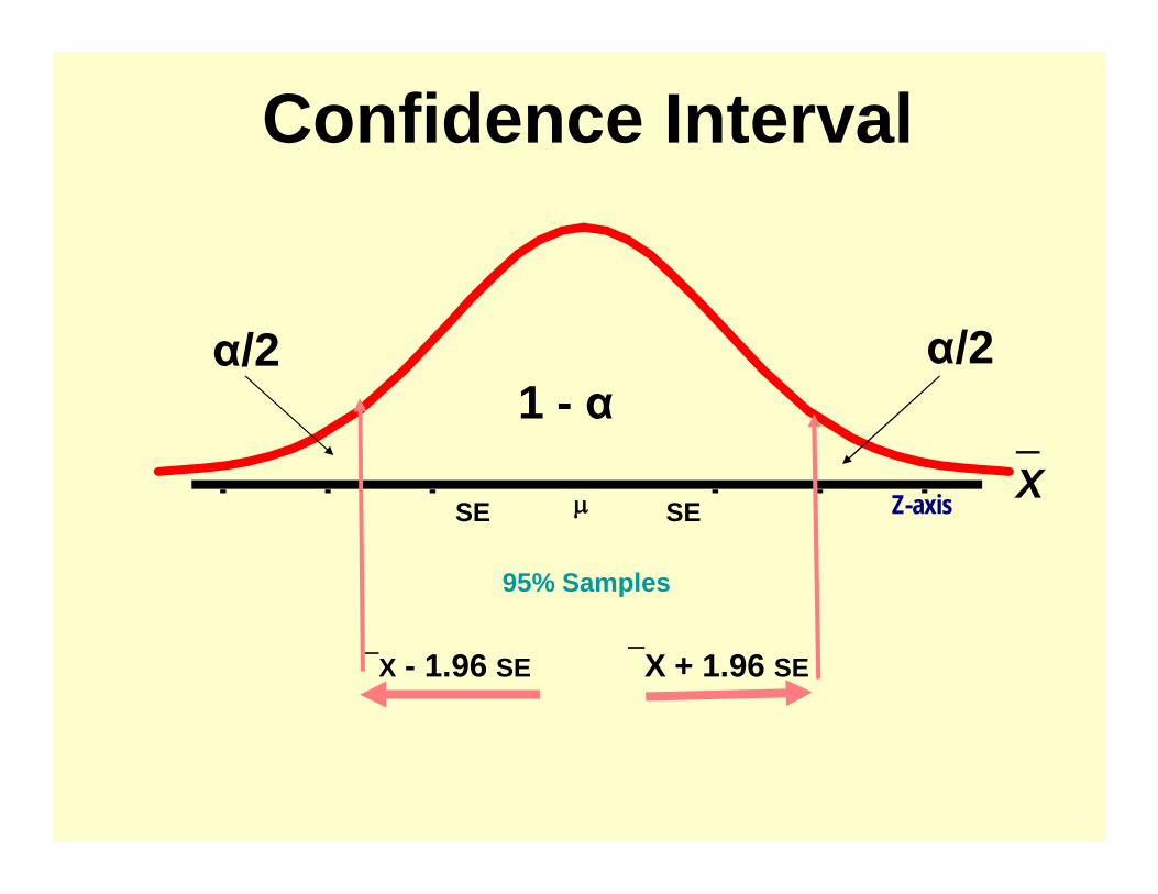
95% Samples
Confidence Interval
X_
X - 1.96 SE X + 1.96 SE
SESE Z-axis
1 - αα/2α/2

95% Samples
Confidence Interval
SESE p
p + 1.96 SEp - 1.96 SE
Z-axis
1 - αα/2α/2

Interpretation of CI
Probabilistic Practical
We are 100(1-)% singleconfident that the
computed CI contains
In repeated sampling 100(1-around all intervals)% of
sample means will in the long run include

Example (Sample size≥30)
An epidemiologist studied the blood glucose level of a random sample of 100 patients. The mean was 170, with a SD of 10.
SE = 10/10 = 1
Then CI:
= 170 + 1.96 1 168.04 171.96
95%
= X + Z SE
In a survey of 140 asthmatics, 35% had allergy to house dust. Construct the 95% CI for the population proportion.
= p + Z
0.35 – 1.96 0.04 ≥ 0.35 + 1.96 0.04
0.27 ≥ 0.4327% ≥ 43%
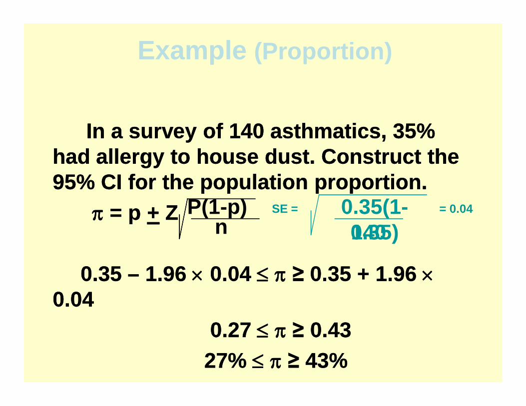
Example (Proportion)
In a survey of 140 asthmatics, 35% had allergy to house dust. Construct the 95% CI for the population proportion.
= p + Z
0.35 – 1.96 0.04 ≥ 0.35 + 1.96 0.04
0.27 ≥ 0.4327% ≥ 43%
P(1-p)n 140
0.35(1-0.35)
= 0.04SE =

Hypothesis testing
A statistical method that usessample data to evaluate ahypothesis about a populationparameter. It is intended to helpresearchers differentiatebetween real and randompatterns in the data.

• H0 Null Hypothesis states the Assumption to be tested e.g. SBP of participants = 120 (H0: = 120).
• H1 Alternative Hypothesis is the opposite of the null hypothesis (SBP of participants ≠ 120 (H1: ≠ 120). It may or may not be accepted and it is the hypothesis that is believed to be true by the researcher
Null & Alternative Hypotheses

• Defines unlikely values of samplestatistic if null hypothesis is true.Called rejection region of samplingdistribution
• Typical values are 0.01, 0.05• Selected by the Researcher at the
Start• Provides the Critical Value(s) of the
Test
Level of Significance, a

Level of Significance, a and the Rejection Region
0
aCritical Value(s)
Rejection Regions

H0: Innocent
Jury Trial Hypothesis Test
Actual Situation Actual Situation
Verdict Innocent Guilty Decision H 0 True H 0 False
Innocent Correct ErrorAccept
H 01 -
Type IIError ( b )
Guilty Error CorrectH 0
Type IError
( )
Power(1 - b )
Result Possibilities
False Negative
False Positive
Reject

• True Value of Population Parameter– Increases When Difference Between
Hypothesized Parameter & True Value Decreases
• Significance Level – Increases When Decreases
• Population Standard Deviation – Increases When Increases
• Sample Size n– Increases When n Decreases
Factors Increasing Type II Error
b
b
b
n
βb d
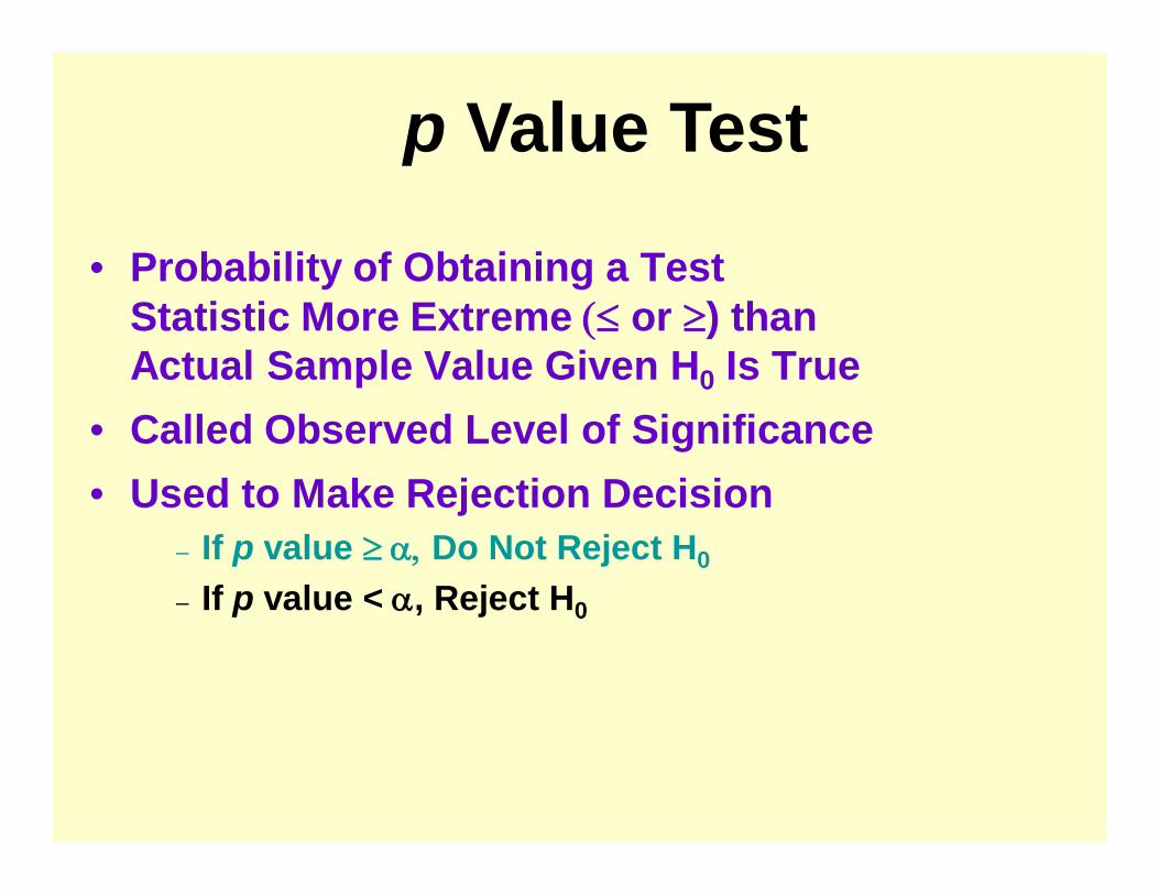
• Probability of Obtaining a Test Statistic More Extreme or ) than Actual Sample Value Given H0 Is True
• Called Observed Level of Significance• Used to Make Rejection Decision
– If p value Do Not Reject H0
– If p value < , Reject H0
p Value Test

State H0 H0 : m = 120
State H1 H1 : m 120
Choose = 0.05
Choose n n = 100
Choose Test: Z, t, X2 Test (or p Value)
Hypothesis Testing: Steps
Test the Assumption that the true mean SBP of participants is 120 mmHg.

Compute Test Statistic (or compute P value)
Search for Critical Value
Make Statistical Decision rule
Express Decision
Hypothesis Testing: Steps

• Assumptions– Population is normally
distributed
• t test statistic
One sample-mean Test
ns
xt 0
error standard valuenullmean sample

Example Normal Body Temperature
What is normal body temperature? Is it actually 37.6oC (on average)?
State the null and alternative hypotheses
H0: = 37.6oC
Ha: 37.6oC

Example Normal Body Temp (cont)Data: random sample of n = 18 normal body temps37.2 36.8 38.0 37.6 37.2 36.8 37.4 38.7 37.236.4 36.6 37.4 37.0 38.2 37.6 36.1 36.2 37.5
Variable n Mean SD SE t PTemperature 18 37.22 0.68 0.161 2.38 0.029
ns
xt 0
error standard valuenullmean sample
Summarize data with a test statistic

STUDENT’S t DISTRIBUTION TABLEDegrees of freedom
Probability (p value) 0.10 0.05 0.01
1 6.314 12.706 63.6575 2.015 2.571 4.03210 1.813 2.228 3.16917 1.740 2.110 2.89820 1.725 2.086 2.84524 1.711 2.064 2.79725 1.708 2.060 2.787 1.645 1.960 2.576

Example Normal Body Temp (cont)
Find the p-valueDf = n – 1 = 18 – 1 = 17From SPSS: p-value = 0.029
From t Table: p-value is between 0.05 and 0.01.
Area to left of t = -2.11 equals area to right of t = +2.11.
The value t = 2.38 is between column headings 2.110& 2.898 in table, and for df =17, the p-values are 0.05 and 0.01.
-2.11 +2.11 t
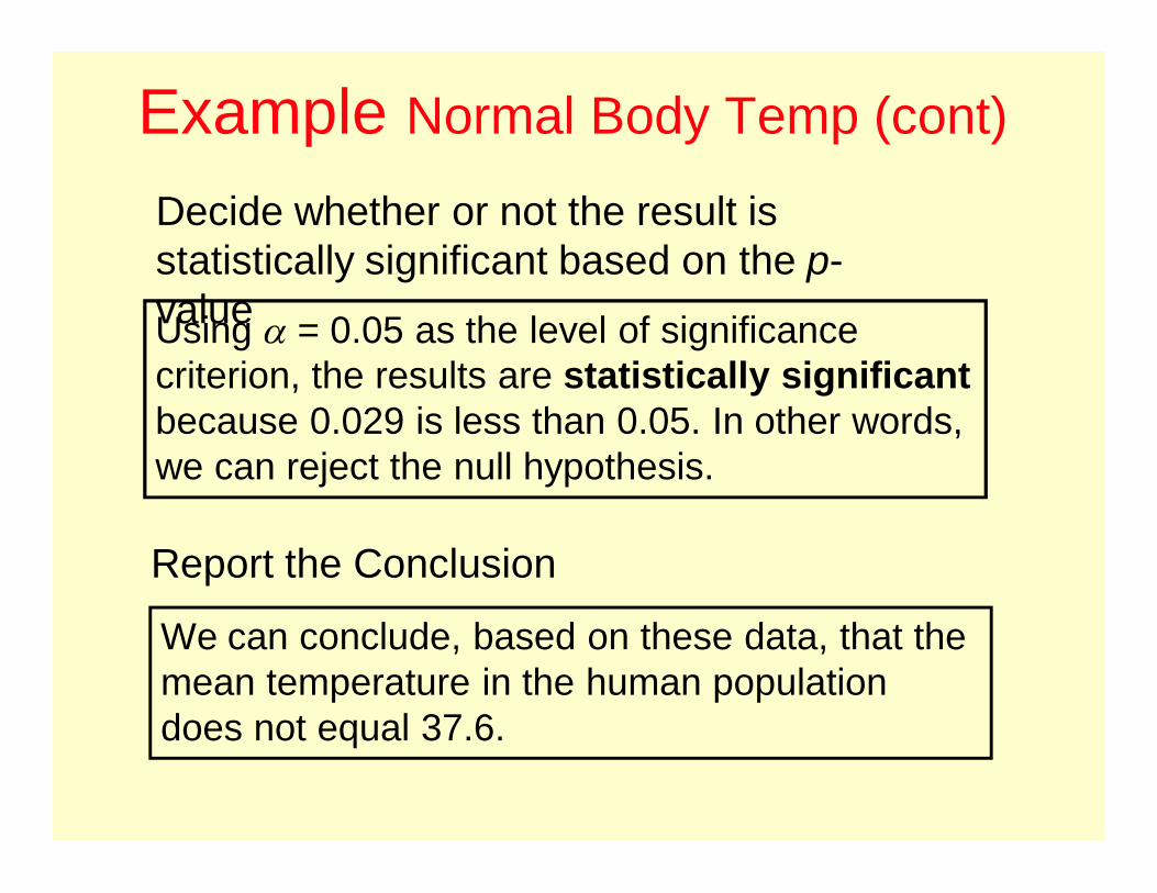
Example Normal Body Temp (cont)
Decide whether or not the result is statistically significant based on the p-valueUsing a = 0.05 as the level of significance criterion, the results are statistically significantbecause 0.029 is less than 0.05. In other words, we can reject the null hypothesis.
Report the Conclusion
We can conclude, based on these data, that the mean temperature in the human population does not equal 37.6.

• Involves categorical variables• Fraction or % of population in a category• Sample proportion (p)
One-sample test for proportion
sizesamplesuccessesofnumber
nXp
n
pZ)1(
Test is called Z test where:
Z is computed value π is proportion in population
(null hypothesis value) Critical Values: 1.96 at α=0.05
2.58 at α=0.01

Example
• In a survey of diabetics in a large city, itwas found that 100 out of 400 have diabeticfoot. Can we conclude that 20 percent ofdiabetics in the sampled population havediabetic foot.
• Test at the =0.05 significance level.

Solution
Critical Value: 1.96
Decision:We have sufficient evidence to reject theHo value of 20%We conclude that in the population ofdiabetic the proportion who havediabetic foot does not equal 0.20
Z0
Reject Reject
.025.025
= 2.50
Ho: π = 0.20
H1: π 0.20 Z =0.25 – 0.20
0.20 (1- 0.20)400
+1.96-1.96


Example
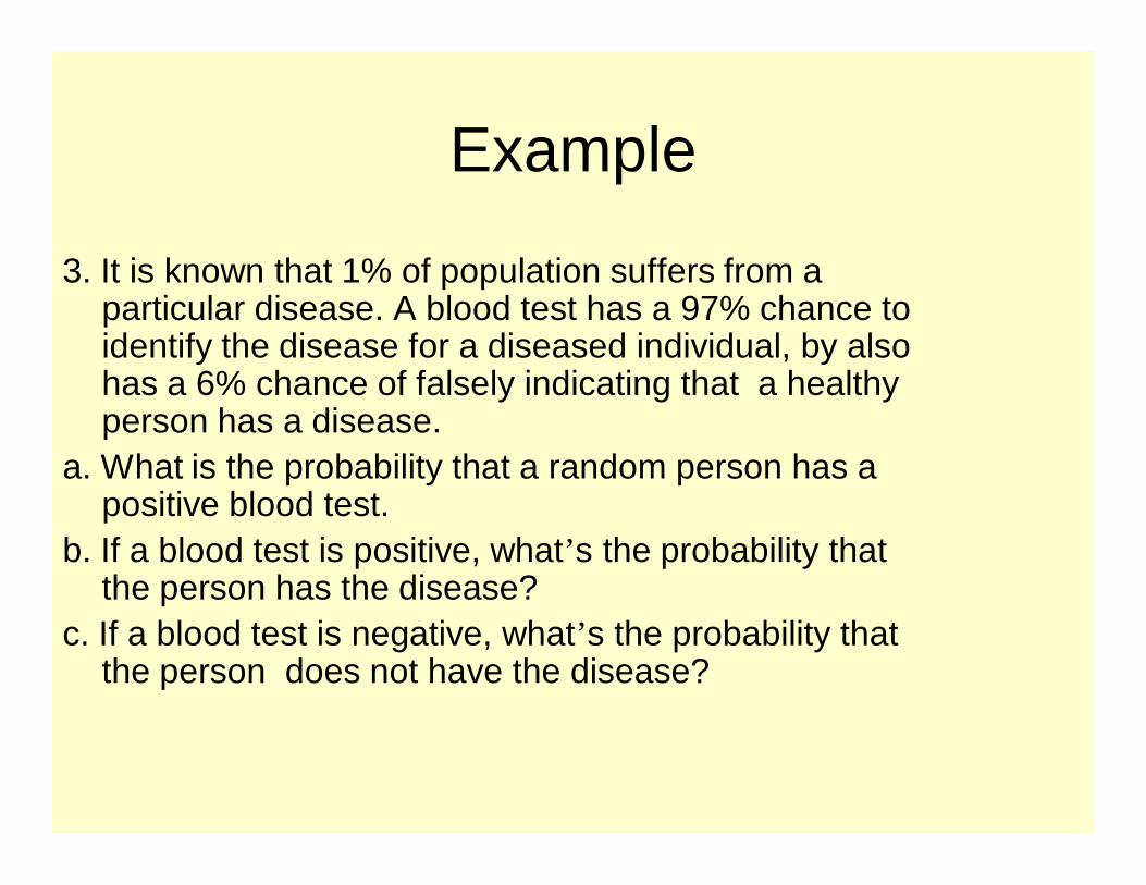
3. It is known that 1% of population suffers from a particular disease. A blood test has a 97% chance to identify the disease for a diseased individual, by also has a 6% chance of falsely indicating that a healthy person has a disease.
a. What is the probability that a random person has a positive blood test.
b. If a blood test is positive, what’s the probability that the person has the disease?
c. If a blood test is negative, what’s the probability that the person does not have the disease?

• A is the event that a person has a disease. P(A) = 0.01; P(A’) = 0.99.
• B is the event that the test result is positive.– P(B|A) = 0.97; P(B’|A) = 0.03;– P(B|A’) = 0.06; P(B’|A’) = 0.94;
• (a) P(B) = P(A) P(B|A) + P(A’)P(B|A’) = 0.01*0.97 +0.99 * 0.06 = 0.0691
• (b) P(A|B)=P(B|A)*P(A)/P(B) = 0.97* 0.01/0.0691 = 0.1403
• (c) P(A’|B’) = P(B’|A’)P(A’)/P(B’)= P(B’|A’)P(A’)/(1-P(B))= 0.94*0.99/(1-.0691)=0.9997
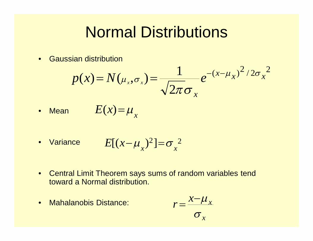
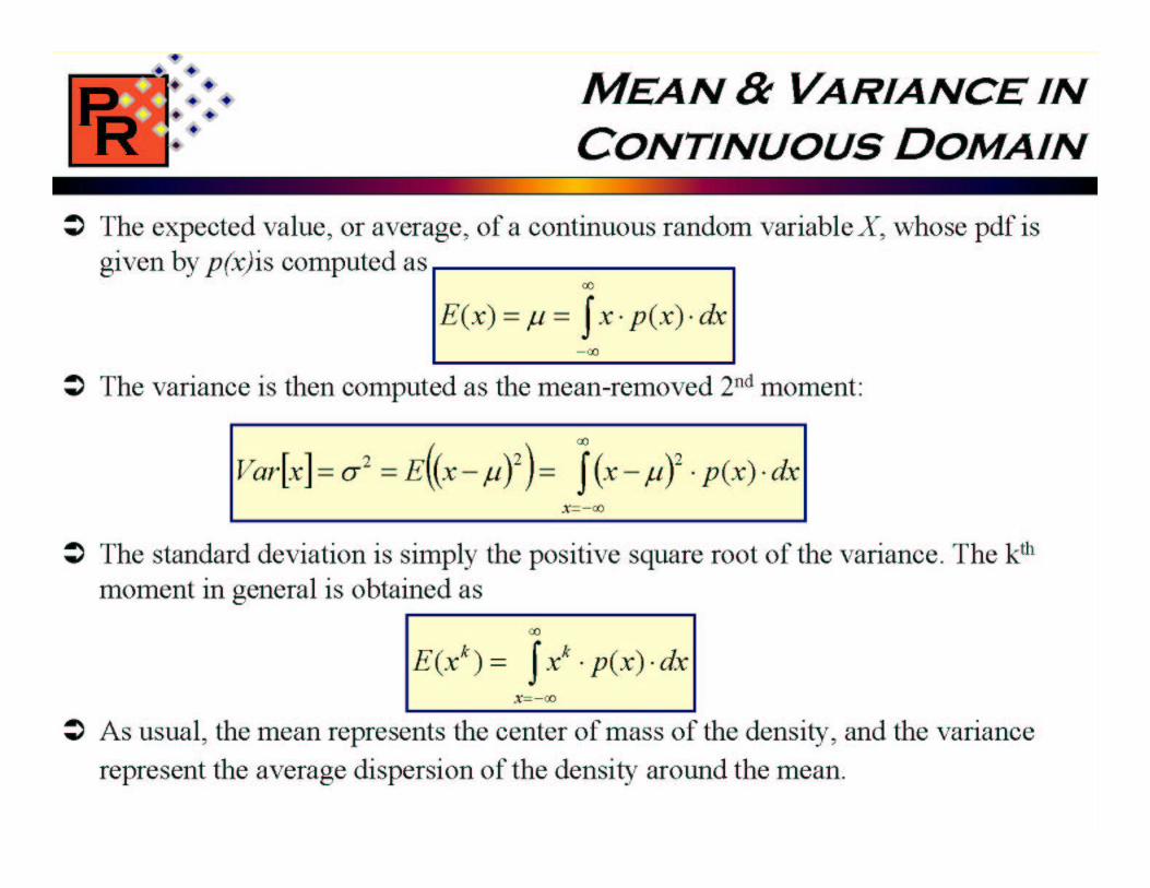
Normal Distributions• Gaussian distribution
• Mean
• Variance
• Central Limit Theorem says sums of random variables tend toward a Normal distribution.
• Mahalanobis Distance:
xxE )(
22/2)(
21),()( xxx
x
eNxp xx
22])[( xxxE
x
xxr
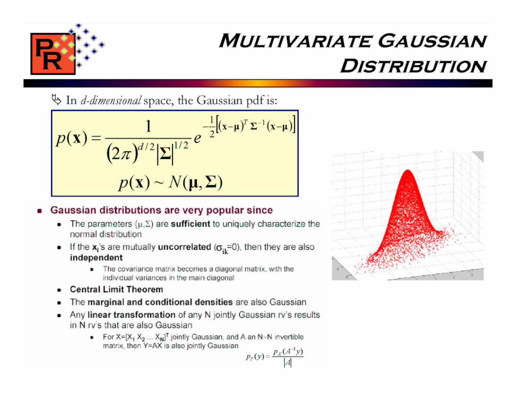

Multivariate Normal Density• x is a vector of d Gaussian variables
• Mahalanobis Distance
• All conditionals and marginals are also Gaussian
dxxpxxxxE
dxxxpxE
xTxedNxp
TT )())((]))([(
)(][
)(1)(21
2/1||2/2
1),()(
)()( 12 xxr T

104
Bayesian Decision Making
Classification problem in probabilistic terms
Create models for how features are distributed for objects of different classes
We will use probability calculus to make classification decisions
105
XY
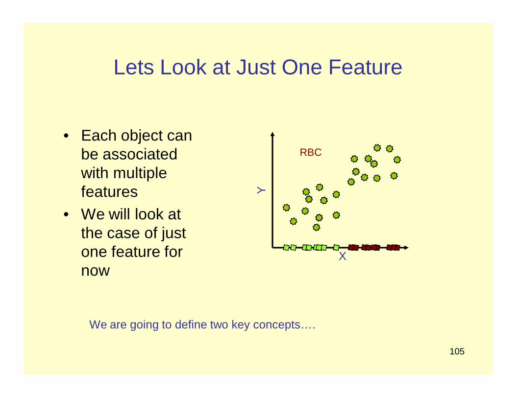
Lets Look at Just One Feature
• Each object can be associated with multiple features
• We will look at the case of just one feature for now
RBC
We are going to define two key concepts….
106
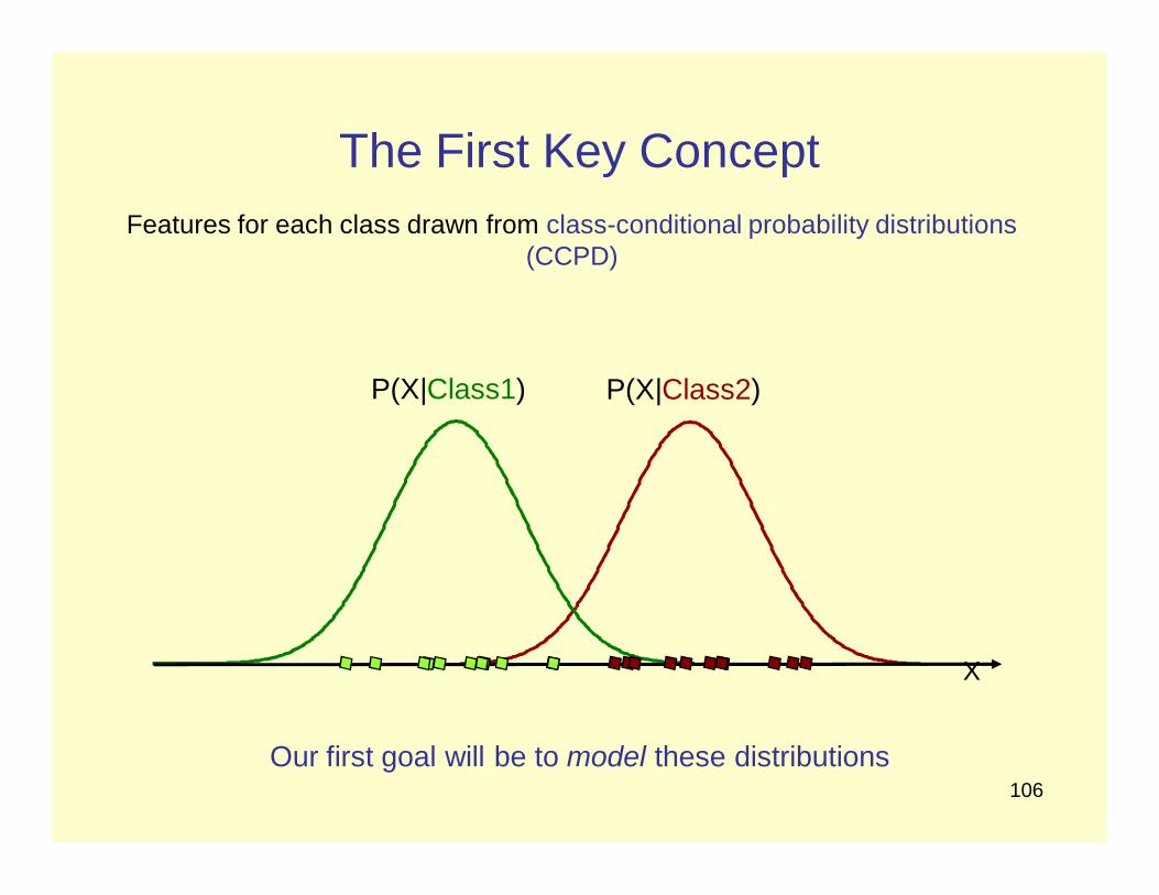
The First Key ConceptFeatures for each class drawn from class-conditional probability distributions
(CCPD)
P(X|Class1) P(X|Class2)
Our first goal will be to model these distributions
X
107
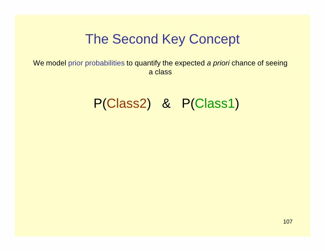
The Second Key ConceptWe model prior probabilities to quantify the expected a priori chance of seeing
a class
P(Class2) & P(Class1)

108
But How Do We Classify?
• So we have priors defining the a priori probability of a class
• We also have models for the probability of a feature given each class
But we want the probability of the class given a featureHow do we get P(Class1|X)?
P(Class1), P(Class2)
P(X|Class1), P(X|Class2)

109
Bayes Rule
( | ) ( )( | )( )
P Feature Class P ClassP Class FeatureP Feature
Prior
Likelihood
PosteriorEvidence
Belief before evidence
Evaluateevidence
Belief after evidence
Bayes, Thomas (1763) An essaytowards solving a problem in thedoctrine of chances. PhilosophicalTransactions of the Royal Society ofLondon, 53:370-418
Copyright@SMST 110
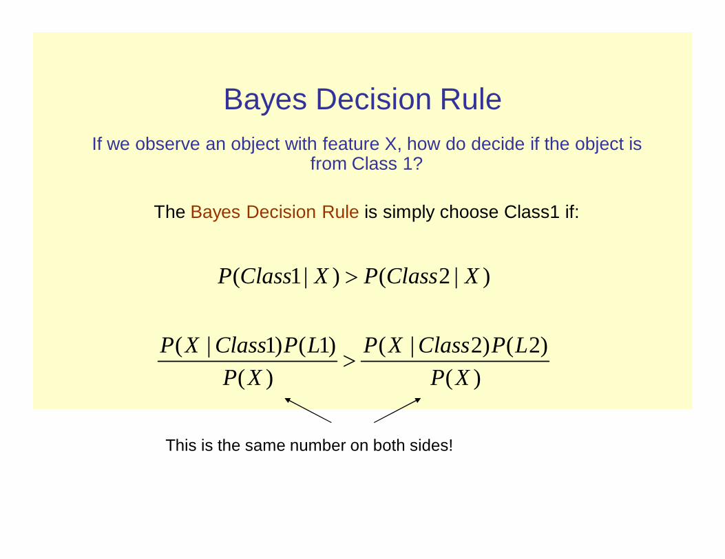
Bayes Decision RuleIf we observe an object with feature X, how do decide if the object is
from Class 1?
The Bayes Decision Rule is simply choose Class1 if:
( 1| ) ( 2 | )
( | 1) ( 1) ( | 2) ( 2)(
( | 1) ( 1) ( | 2) (
) )
)
(
2
P Class X P Class X
P X Class P L P X Class
P X Class P Class P X
P LP X P X
Class P Class
This is the same number on both sides!

111
Discriminant FunctionWe can create a convenient representation of the
Bayes Decision Rule
( | 1) ( 1) ( | 2) ( 2)
( | 1) ( 1) 1( | 2) ( 2)
( | 1) ( 1)( ) log 0( | 2) ( 2)
P X Class P Class P X Class P Class
P X Class P ClassP X Class P Class
P X Class P ClassG XP X Class P Class
If G(X) > 0, we classify as Class 1

112
Stepping back
( | ) ( )1 1( ) log 0( | ) ( )2 2Cla
Class Classss Clas
P X PG XP sX P
Given a new feature, X, we plug it into this equation…
…and if G(X)> 0 we classify as Class1
What do we have so far?
P(X|Class1), P(X|Class2) P(Class1), P(Class2)
We have defined the two components, class-conditional distributions and priors
We have used Bayes Rule to create a discriminant function for classification from these components

113
Getting P(X|Class) from Training SetP(X|Class1)
One Simple Approach
Divide X values into bins
And then we simply count frequencies
<1 1-3 3-5 5-7 >7
2/13
0
7/13
3/13
1/13
There are 13 data points
X
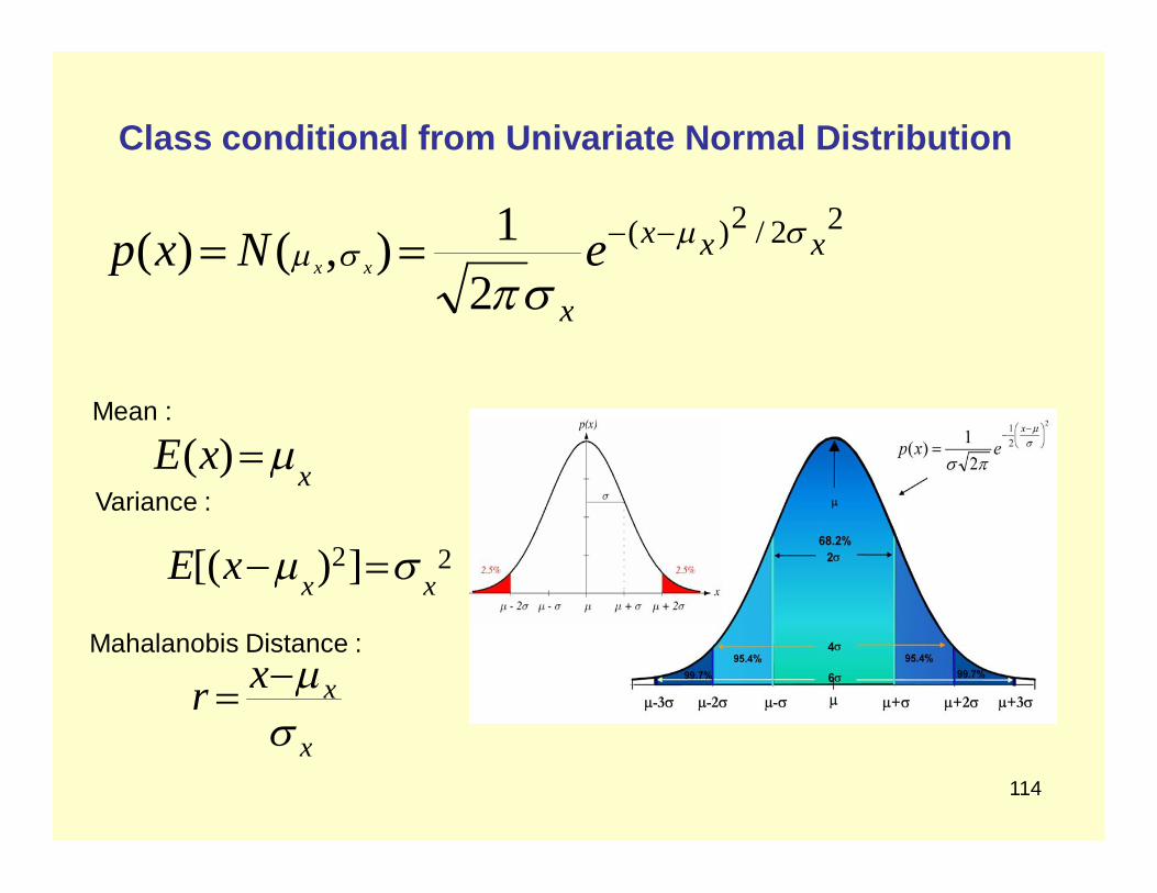
Class conditional from Univariate Normal Distribution
114
22/2)(
21),()( xxx
x
eNxp xx
xxE )(
22])[( xxxE
x
xxr
Mean :
Variance :
Mahalanobis Distance :

115
We Are Just About There….We have created the class-conditional distributions and priors
( | ) ( )1 1( ) log 0( | ) ( )2 2Cla
Class Classss Clas
P X PG XP sX P
P(X|Class1), P(X|Class2) P(Class1), P(Class2)
And we are ready to plug these into our discriminant function
But there is one more little complication…..

116
Multidimensional feature space ?So P(X|Class) become P(X1,X2,X3,…,X8|Class)
and our discriminant function becomes
1 2 7
1 2 7
( , ,..., | ) ( )( ) log 0( , ,. 2.., | ) ( )
1 12Class
Class ClasP X X XCla
ss
PG XP X X sX P
117
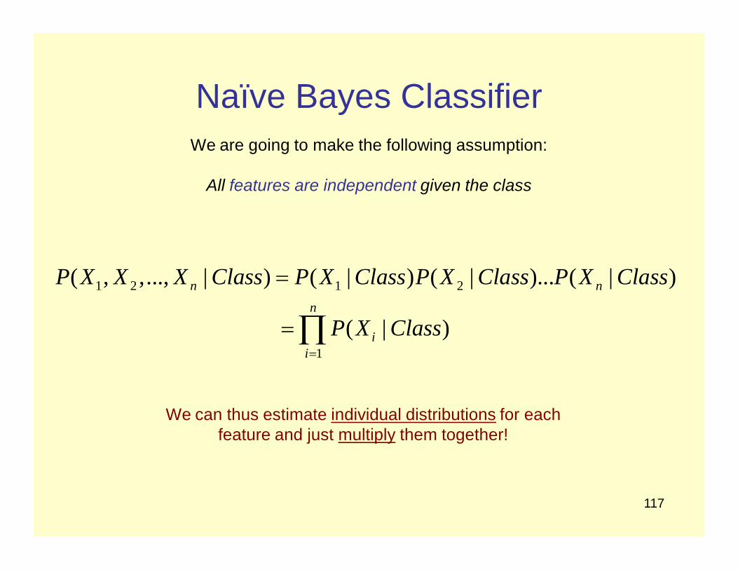
Naïve Bayes ClassifierWe are going to make the following assumption:
All features are independent given the class
1 2 1 2
1
( , ,..., | ) ( | ) ( | )... ( | )
( | )
n nn
ii
P X X X Class P X Class P X Class P X Class
P X Class
We can thus estimate individual distributions for eachfeature and just multiply them together!

118
Naïve Bayes Discriminant Function
1 2 71 7
1 2 7
( , ,..., | ) ( )1( ,..., ) log 0( , ,..., |
1(2 2) )
P X X X PG X XP X
ClassClass ClasX sX
ssP
Cla
1 7
( | ) ( )( ,..., ) log 0( | ) (2 2)
1 1i
i
P X PG X XP X
ClassClass ClasP
Classs
Thus, with the Naïve Bayes assumption, we can now rewrite, this:
As this:
119
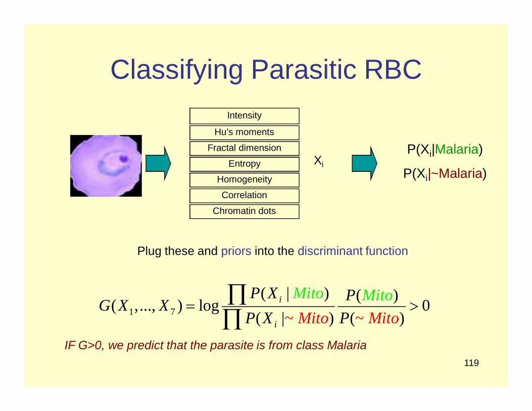
Classifying Parasitic RBC
1 7
( | ) ( )( ,..., ) log 0( | )~ )~(
i
i
Mito MitoP X PG X XP Mito P oX Mit
Plug these and priors into the discriminant function
IF G>0, we predict that the parasite is from class Malaria
Intensity
Hu’s moments
Entropy
Fractal dimension
Homogeneity
Correlation
Chromatin dots
P(Xi|Malaria)
P(Xi|~Malaria)Xi
120
How Good is the Classifier?
The RuleWe must test our classifier on a different set
from the training set: the labeled test set
The TaskWe will classify each object in the test set
and count the number of each type of error

121
Binary Classification Errors
• Sensitivity– Fraction of all Class1 (True) that we correctly predicted at Class 1– How good are we at finding what we are looking for
• Specificity– Fraction of all Class 2 (False) called Class 2– How many of the Class 2 do we filter out of our Class 1 predictions
True (Mito) False (~Mito)
Predicted True TP FPPredicted False FN TN
Sensitivity = TP/(TP+FN) Specificity = TN/(TN+FP)
In both cases, the higher the better

Thank you