1

Lecture 5:Fundamentals of Solid Mechanics for

Packaging Applications

Sören Östlund

After Lecture 5 you should be able to

• discuss the mechanical behaviour of packaging materials, particularly paper and board, in terms of thematerials, particularly paper and board, in terms of the most important types of concepts used in solid mechanics.

2

SOLID MECHANICSEquations relating field Variables

• Equations of Motion (Equilibrium)Equations of Motion (Equilibrium)– Relating external forces to internal forces (stresses) in the

material

• Strain-Displacement Relations (Compatibility)– Relates deformation with strain

C tit ti (St St i ) R l ti• Constitutive (Stress-Strain) Relations– Relates stresses to strains

(More challenging, different equations often used for various problems - even for the same material)

THE CONCEPT OF STRESSTHE CONCEPT OF STRESS

3

STRESSSectioning plane through loaded body

Loaded body

P n

Sectioning plane through point of interest P

STRESSInternal forces on exposed surface

Di t ib ti f i t l f i d f ilib iDistribution of internal forces required for equilibrium

P

RF

P

RM

The stress at point P is the internal force per unit area(internal force intensity) at point P

4

STRESSDefinition - Arbitrary plane

Stress Vector

P

ΔFnS

nFΔ

tFΔnσ

nτ

n

t n n n0limA A

σ τΔ →

Δ= = +

ΔFS n t

Stress Vector

Stress Components (Cauchy)

nli FΔ

AΔ

nn 0

limA

σAΔ →

=Δ

tn 0

limA

FτAΔ →

Δ=

Δ

Normal Stress:

Shear Stress:

STRESSDiscussion of definition

• Stress is a point quantity - evaluated in the limit as the area approaches zero size

• Historically, stress vectors are resolved into normal and shear componentsbecause:

– They cause different types of localized deformations (strains) in most materials (normal stresses are typically related to length changes and shear stresses are typically related to angular changes)

– They have different influences on material failure in various materials

• The stress components will depend on the normal to the sectioning plane• The stress components will depend on the normal to the sectioning plane chosen at the point

5

STRESSDefinition for the coordinate axis planes

Stress componentsFor example, pick the plane with: 1ˆn e=

111 0

limA

FA

σΔ →

Δ=

ΔNormal stress:

Shear stresses: 212 0

limA

FA

σΔ →

Δ=

Δ

3lim Fσ Δ=

ΔF

n 1F FΔ = Δ1x

2x

2FΔ

Δ

tFΔ

p , p p 1

ˆn e 13 0limA A

σΔ →

=ΔP

AΔ3x

3FΔ1n e=

STRESSNotation for the coordinate axis planes

2x Using Newton’s 2nd Lawfor rotational Motion,it b d th t

22σ

1x3x

it can be proved that:

12 21

13 31

23 32

σ σσ σσ σ

==

=32σ

31σ

23σ21σ

13σ

12σ

11σ

11 12 13 11 12 13

21 22 23 12 22 23

31 32 33 13 23 33

σ σ σ σ σ σσ σ σ σ σ σσ σ σ σ σ σ

⎡ ⎤ ⎡ ⎤⎢ ⎥ ⎢ ⎥= =⎢ ⎥ ⎢ ⎥⎣ ⎦ ⎣ ⎦

σNormal stress signs:Positive = TensionNegative = Compression

33σ31

Symmetric 2nd order component matrix:

6

STRESSPlane Stress States

A point is in a state of plane stress if one of the three coordinate planes is stress free

22σ

12σ

22σ

12σ

33 31 32 0σ σ σ= = =

13 23 0σ σ→ = =

12σ

11σ

12σ

11σ

STRESSTransformation equations (2D)

Jämvikt ger:

( )

( )

2 2cos sin 2 sin cos

sin 2 cos 22

x y xy

y xxy

σ ϕ σ ϕ σ ϕ τ ϕ ϕ

σ στ ϕ ϕ τ ϕ

= + +

−= +

7

STRESSPrincipal stresses

Considering all directions, the maximum and minimum normal stresses at a point (and their associated directions) can be

11 12 13

12 22 23

13 23 33

σ σ σσ σ σσ σ σ

⎡ ⎤⎢ ⎥=⎢ ⎥⎣ ⎦

σ

stresses at a point (and their associated directions) can be found by finding the eigenvalues and eigenvectors of the symmetric 3 x 3 matrix of stress components:

13

max minmax 2abs

σ στ −

−=

The maximum shear stress at point can be found from the maximum and minimum normal stresses at the point:

SOLID MECHANICSEquations of motion

2∂∂ ∂ ∂

m=∑F a2

1311 12 11 1 2

1 2 32

2312 22 22 2 2

1 2 32

13 23 33 3

uf ax x x t

uf ax x x t

uf a

σσ σ ρ ρ

σσ σ ρ ρ

σ σ σ ρ ρ

∂∂ ∂ ∂+ + + = =

∂ ∂ ∂ ∂

∂∂ ∂ ∂+ + + = =

∂ ∂ ∂ ∂

∂ ∂ ∂ ∂+ + + = =

12 21

13 31

23 32

σ σσ σσ σ

===

Reminder

3 3 21 2 3

f ax x x t

ρ ρ+ + + = =∂ ∂ ∂ ∂

321 f,f,f are body force components per unit volume

321 a,a,a are the acceleration components of the point

8

THE CONCEPT OF STRAINTHE CONCEPT OF STRAIN

STRAINDefinition - "Engineering” Strain

Deformed body 2s′Δ

θP′

2x

Undeformed body

P

P′1s′Δ

3s′Δ

12θ23θ

13θ

P′

1x

3x

3e1e

2e

1sΔ

2sΔ

3sΔ

P

9

STRAINDefinition - "Engineering” Strain

Normal strains

2s′Δ

12θ23θP′

1sΔ

2sΔ

3sΔ

P1

1 111 0

1

lims

s ss

εΔ →

⎡ ⎤′Δ − Δ= ⎢ ⎥Δ⎣ ⎦

2

2 222 0

2

lims

s ss

εΔ →

⎡ ⎤′Δ − Δ= ⎢ ⎥Δ⎣ ⎦

s s⎡ ⎤′Δ Δ1s′Δ

3s′Δ 13θ

Normal strain = Change in length divided by original lengthfor an infinitesimal line segment at a point

3

3 333 0

3

lims

s ss

εΔ →

⎡ ⎤Δ −Δ= ⎢ ⎥Δ⎣ ⎦

STRAINDefinition - "Engineering” Strain

Shear strains

1 212 12 12, 0

2 lim2s s

πε γ θΔ Δ →

⎡ ⎤≡ = −⎢ ⎥⎣ ⎦

1 313 13 13, 0

2 lim2s s

πε γ θΔ Δ →

⎡ ⎤≡ = −⎢ ⎥⎣ ⎦

23 23 232 lim πε γ θ⎡ ⎤≡ = −⎢ ⎥⎣ ⎦

2s′Δ

12θ23θP′

1sΔ

2sΔ

3sΔ

P

Shear strain = Change in angle of an originally orthogonal set ofdirections at a point

2 323 23 23, 0 2s s

γΔ Δ → ⎢ ⎥⎣ ⎦ 1s′Δ

3s′Δ 13θ

10

STRAINNormal strain in x-direction

x x+Δxx x+Δx

( )xu x ( )xu x x+ Δ( )x

( ) ( )( ) ( )x x xx

u x x u x dux xx dx

ε + Δ −= =

Δ

SOLID MECHANICSStrain-Displacement Relations

For small strains, we can use the linearized version of thestrain-displacement equations and the engineering strain components:

111

1

ux

ε ∂=∂

2 112 12

1 2

2 u ux x

ε γ ∂ ∂= = +

∂ ∂

12

jiij

j i

uux x

ε⎡ ⎤∂∂

= +⎢ ⎥∂ ∂⎢ ⎥⎣ ⎦

222

2

333

3

uxux

ε

ε

∂=∂∂

=∂

1 2

3113 13

3 1

3223 23

3 2

2

2

uux x

uux x

ε γ

ε γ

∂∂= = +

∂ ∂∂∂

= = +∂ ∂

11

STRAINPrincipal strains

Considering all directions, the maximum and minimum normal strains at a point (and their associated directions) can be

11 12 13

12 22 23

13 23 33

ε ε εε ε εε ε ε

⎡ ⎤⎢ ⎥= ⎢ ⎥⎢ ⎥⎣ ⎦

ε

strains at a point (and their associated directions) can be found by finding the eigenvalues and eigenvectors of the symmetric 3 x 3 matrix of strain components:

max max minabsγ ε ε− = −

The maximum shear strain at point can be found from the maximum and minimum normal strains at the point:

CONSTITUTIVE EQUATIONSCONSTITUTIVE EQUATIONS

12

CONSTITUTIVE MODELSGeneral Comments

• Constitutive equations describe the macroscopic behaviour resulting from the internal constitution of thebehaviour resulting from the internal constitution of the material.

• Often they are phenomenological / empirical in that they represent the observed phenomena without understanding the underlying details from which they result (curve fits).

• In solid mechanics, the constitutive relations are typically stress-strain relations.

We Need Some Experimental Data!!

CONSTITUTIVE MODELSApproaches for Development

• It is not feasible to write down one equation or one set of equations that accurately models a realset of equations that accurately models a real material over its entire range of behaviour.

• Typically, separate theories are formulated for various kinds of ideal material response. Each formulation is designed to approximate physical observations of the response of a material over a

it bl f b h isuitable range of behaviour.

13

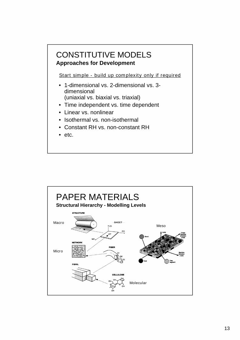
CONSTITUTIVE MODELSApproaches for Development

Start simple - build up complexity only if required

• 1-dimensional vs. 2-dimensional vs. 3-dimensional(uniaxial vs. biaxial vs. triaxial)

• Time independent vs. time dependent• Linear vs. nonlinear• Isothermal vs. non-isothermal• Constant RH vs. non-constant RH• etc.

PAPER MATERIALSStructural Hierarchy - Modelling Levels

SHEETMacro SHEETMacro

Micro

Meso

Molecular

14

SOLID MECHANICSTypes of constitutive (stress-strain) relations

• Elastic– The material is like a spring - all deformations arep g

recovered when the loading is removed• Plastic

– Permanent deformations occur which are non-recoverable• Elastic-plastic

– The material is first elastic, and then elastic-plastic• Viscoelastic

– The material experiences elastic and viscous (time dependent) deformations

• Viscoplastic– Combines viscoelastic and plastic behaviors

• Continuum damage– Considers development of damage in the structure

CONSTITUTIVE MODELSMaterial Characterization Experiments

U i i l t i d/ i t t

Basic experiments (application of uniform stress/strain)

• Uniaxial tension and/or compression test• Pure shear test (not necessarily so-basic)• Creep test• Stress relaxation test• Cyclic uniaxial testing

• Bending tests (non-uniform stress / strain)• Biaxial tests (hard to do)

Not-so-basic experiments

15

BASIC MEASUREMENTS BASIC MEASUREMENTS (STIFFNESS, STRENGTH, etc.)

UNIAXIAL TESTINGSpecimen Geometry and Loading

Unloaded Specimen b

Loaded Specimen

Lt

tbA =

b′ PP

3x

1x2x

Assume uniform deformations in the loaded specimen

L′

PPt′

tbA ′′=′

16

UNIAXIAL TESTINGTension and Compression

• Tests are normally run in either displacement (stroke) control or load controlcontrol or load control– Displacement control: The cross-heads which hold the specimen

grips separate at a constant rate. Thus the axial strain in the specimens changes at a constant rate.

– Load control: The load applied to the specimen is increased at a constant rate.

• Typically the load on the specimen is monitored with a

1C tε =

2C tσ =y y

load cell (force transducer) and the relative motion of the cross-heads is monitored (change in length of the specimen).

UNIAXIAL TESTINGAxial Stress

PF =P

P

tbA ′′=′

AP

AP≈′

=11σ

Average axial stress

Engineering

The stress is assumed to be uniformly distributed over the cross-sectional area

3x

True stressstress

3

1x2x

AP

=11σ

P P

3x

1x2x

At any point in the specimen:

17

UNIAXIAL TESTINGDeformations and Strains

3x

1x

LLL −′=Δ≡δ

LLL

LLL δε =

Δ=

−′=11

Average axial strain

12x

Extension

LLL

bb

bbb Δ=

−′=22ε

Average transverse strains

tt

ttt Δ=

−′=33ε

PAPERTypical Load vs. Extension Data

P

PuFracture

P,Load k

Linear Region

δ,Extension uδ

δkP =

P

18

PAPERTypical Axial Stress vs. Axial Strain Data

Stress-strain curve

AP

=σ

Ultimate strength

Proportional limit,or yield Stress

In the linear region

εσ E=

δ⎟⎞⎜⎛=

AEP

LE

AP δ=

Lδε =

Ultimate strain

E, Elastic modulus = Young’s modulusδ⎟⎠

⎜⎝

=L

P

LAEk =

1

PAPERPoisson’s Ratio Data

3x

1x2x LL

LL

LL δε =Δ

=−′

=11

= Poisson s ratioν2 LLL

22ε

se S

trai

n

bb

bbb Δ=

−′=22ε

1122 ενε −=

In the linear region

11ε

Axial Strain

Tran

sver

s

From the stress-strain curve

1111 εσ E=This gives:

E11

22σνε −=

19

PAPERAnisotropic (Orthotropic) Material Behavior

θ

CD

Specimen Orientation

θ

θ

MD

PAPERStress-Strain Curve - Plasticity Effects

Elastic-plastic behaviorIf the stress becomes higher thanthe yield stress (the stress-straincurve becomes nonlinear), permanentstrains are obtained when unloadingthe specimen. The unloading curveand reloading curves are essentiallyparallel to the initial linear response.

σYσ

20

PAPERStress-Strain Curve – Rate Dependent Behaviour

Variation of the stress-strain curve with extension-rate

PAPERThickness Variation

t

21

PAPERThickness Measurement

• Since the thickness is variable, an average value is typically used in the stress calculations for theis typically used in the stress calculations for the basic experimental tests (uniaxial testing and shear testing in torsion)

• In some laboratories, the “stress” in a stress-strain curve is calculated in units of force per unit width instead of force per unit areawidth instead of force per unit area.

btP

AP==σ

bPb =σ

Stress Force per unit width

PAPERSpecific stress

P P

Stress

A btσ = =

b Pb

σ =

Force per unit width

bw t P

w w bw wt

σ σ σ σσρ

= = = = =⎛ ⎞⎜ ⎟⎝ ⎠

Specific stress

w = grammage /basis weight

22

TENSIONNotation for Paper Elastic Moduli

Coordinate axis convention(for paper, wood, composites)

1E

2E MDx =1 CDx =2

ZDx =3

ZD

CD

MD

EEEEEE

≡≡≡

3

2

1

Typical stress-strain curve for a 150 g/m2 fluting

23

Typical stress-strain curve for a 180 g/m2 liner

Paperboard

MD

45o

CD

MD -shear

CD -shear

ZD

24

Load-strain curvesSack paper and newsprint

Sack paper

Newsprint

Nordman (1969)

TENSIONTypical Effects of Moisture Content

25

TENSIONTypical Effects of Temperature

COMPRESSIONComparison of tensile and compressive curves

There is no widely used method in industry for evaluating the compres-sive stress-strain curve or compressive elastic modulus (buckling problem)

1. The elastic modulus isconstant through theconstant through theorigin.

2. Compressive strengthsare much less thantensile strengths.

26

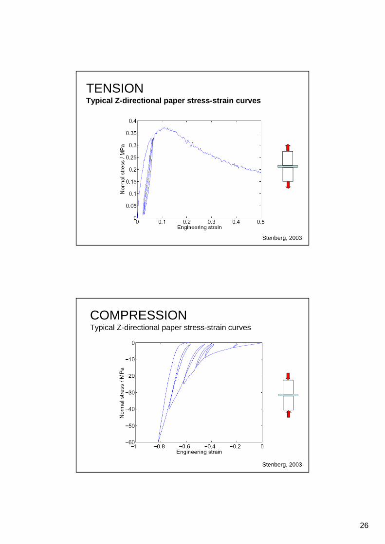
TENSIONTypical Z-directional paper stress-strain curves

Stenberg, 2003

COMPRESSIONTypical Z-directional paper stress-strain curves

Stenberg, 2003

27

SHEAR TESTINGMethods

Stress strain curves

Research approaches ( Still VERY little in industry)

• Stress-strain curves– Torsion of paper cylinders– Arcan test– Rail shear (interlaminar)– Double Notch Shear

• Initial shear modulus

Pure shear (linear region)

γτ G=

• Initial shear modulus– Torsion pendulum– Off-axis tensile test– Ultrasonics

BENDING

28

BENDINGInternal forces and moments in a beam

PP

F = Axial forceP T

F T = Shear forceM = Bending moment

0=∑F0F

T PM Px

===

FMx

BENDINGTypical paper failure in bending

29

BENDINGTheory assumption

“Plane sections remain plane”

A section in pure bending deformsapproximately into a circular arc.

BENDINGTheory

Small element in pure bending

Cross-sectional area

L

x

yz

tb

yz

p g

30

BENDINGTheory

z

x

y

R

From geometrical considerations:

Rz

xx =ε

Assuming linear elastic behavior:

RzEE x

xxxxx == εσ

Assuming linear elastic behavior:

R = radius of curvature of the deformed beam

σ

εE

BENDINGTheory

Cross-sectional area

Using equilibrium arguments

yyx IEM

R==

1κt

b

yCombining:

Mzz

3

121 btI yy =

Area moment of inertiaIEx

xx =ε

IMz

xx =σ

31

BENDINGNon-uniform stress and strain distributions

BENDINGConcept of bending stiffness

⎞⎛ 1 Eκyyxyyx IE

RIEM =⎟

⎠⎞

⎜⎝⎛=

1 3" "12

xx yy

ES EI E I bt≡ = =

Is called the bending stiffness of thebeam and it is the slope of the momentvs. curvature relation.

B di iff i id h

3

12tE

bSS x

b =≡

Bending stiffness per unit width

32

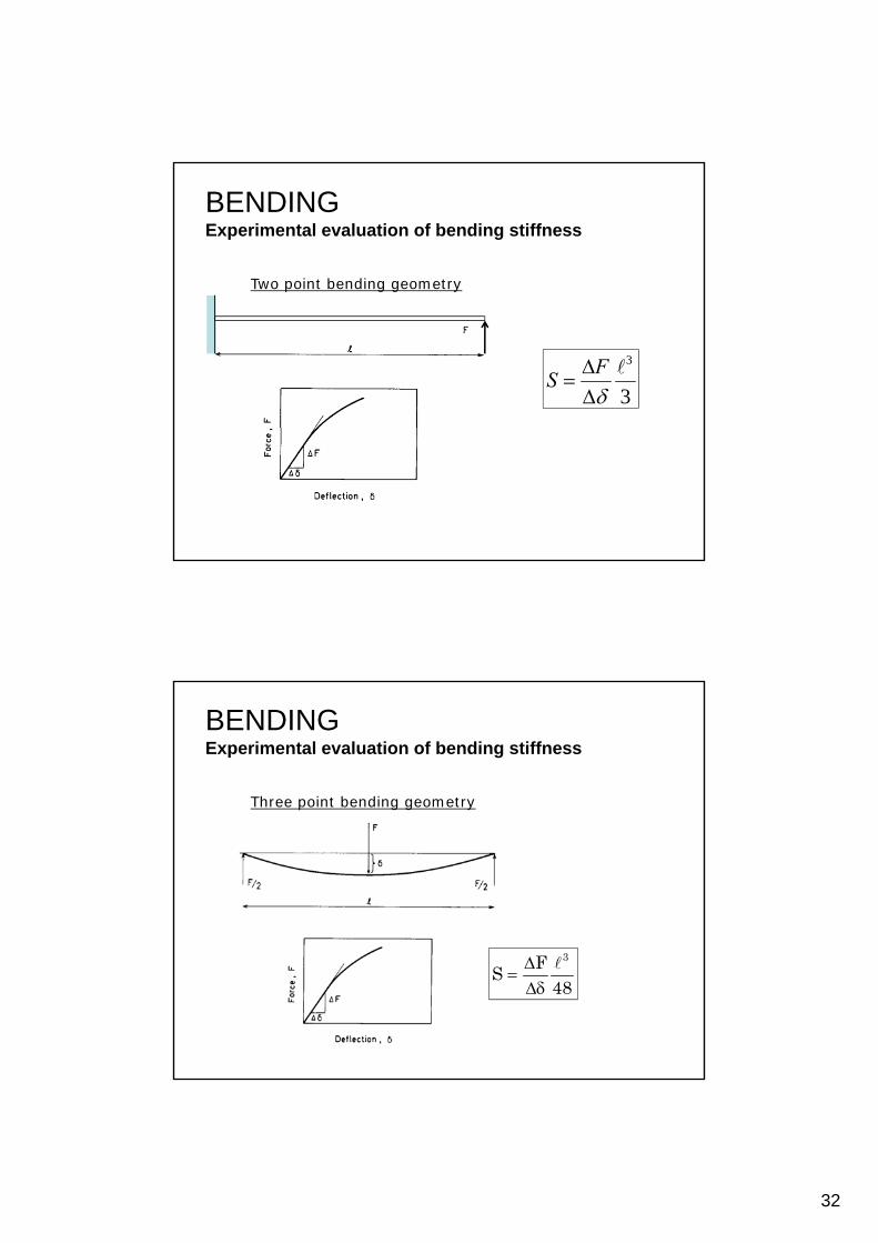
BENDINGExperimental evaluation of bending stiffness

Two point bending geometry

3

3FSδ

Δ=Δ

BENDINGExperimental evaluation of bending stiffness

Three point bending geometry

48FS

3

δΔΔ

=

33

BENDINGExperimental Evaluation of Bending Stiffness

Four point bending geometry

16FS

221

δΔΔ

=

BENDINGExperimental Evaluation of Bending Stiffness

C til b b di ib ti t

242 tf4 ρπ

Cantilever beam bending vibration geometry

66

4)875.1(tf4S ρπ

=

34

Torsion

TLk

θ =k

k = GK for an isotropic material, where G is the shear modulus and K depends on the geometry of the cross-section.

PAPER LINEAR ELASTICITY

35

ELASTICITYGeneral Linear Elastic Stress-Strain Relations

11 12 13 14 15 1611 11 S S S S S Sε ε ⎡⎧ ⎫ ⎧ ⎫ 11σ⎤ ⎧ ⎫11 12 13 14 15 1611 11

21 22 23 24 25 2622 22

31 32 33 34 35 3633 33

41 42 43 44 45 4613 13

51 52 53 54 55 5623 23

222

S S S S S SS S S S S SS S S S S SS S S S S SS S S S S SS S S S S S

ε εε εε εγ εγ εγ ε

⎡⎧ ⎫ ⎧ ⎫⎢⎪ ⎪ ⎪ ⎪⎢⎪ ⎪ ⎪ ⎪⎢⎪ ⎪ ⎪ ⎪⎪ ⎪ ⎪ ⎪= = ⎢⎨ ⎬ ⎨ ⎬⎢⎪ ⎪ ⎪ ⎪

⎪ ⎪ ⎪ ⎪⎪ ⎪ ⎪ ⎪⎪ ⎪ ⎪ ⎪⎩ ⎭ ⎩ ⎭ ⎣

11

22

33

13

23

σσσσσσ

⎤ ⎧ ⎫⎥ ⎪ ⎪⎥ ⎪ ⎪⎥ ⎪ ⎪⎪ ⎪⎥ ⎨ ⎬⎥ ⎪ ⎪

⎢ ⎥ ⎪ ⎪⎢ ⎥ ⎪ ⎪⎢ ⎥ ⎪ ⎪⎩ ⎭⎦61 62 63 64 65 6612 122 S S S S S Sγ ε⎪ ⎪ ⎪ ⎪⎩ ⎭ ⎩ ⎭ ⎣ 12σ⎢ ⎥ ⎪ ⎪⎩ ⎭⎦

are the compliance coefficients (material properties)that must be determined by experimental testing

ijS

ELASTICITYElastic Constants for Orthotropic Materials

MD uniaxial testing (theory)

11 12 1311 11

12 22 2322

13 23 3333

4413

5523

6612

0 0 00 0 0 00 0 0 0

0 0 0 0 0 00 0 0 0 0 00 0 0 0 0 0

S S SS S SS S S

SS

S

ε σεεγγγ

⎡ ⎤⎧ ⎫ ⎧ ⎫⎢ ⎥⎪ ⎪ ⎪ ⎪⎢ ⎥⎪ ⎪ ⎪ ⎪⎢ ⎥⎪ ⎪ ⎪ ⎪⎪ ⎪ = ⎢ ⎥⎨ ⎬ ⎨ ⎬⎢ ⎥⎪ ⎪ ⎪ ⎪⎢ ⎥⎪ ⎪ ⎪ ⎪⎢ ⎥⎪ ⎪ ⎪ ⎪⎢ ⎥⎪ ⎪ ⎩ ⎭⎩ ⎭ ⎣ ⎦

11 11 11

22 12 11

33 13 11

13 23 12 0

SSS

ε σε σε σγ γ γ

===

= = =

C i t t f ti b dComparing our two sets of equations basedon experimental data and theory gives:

111

1SE

= 1212

1

SEν

= − 1313

1

SEν

= −

36

ELASTICITYElastic Constants for Orthotropic Materials

Stress-strain relations for orthotropic material( li ffi i t i t f t i l t t )(compliance coefficients in terms of material constants)

2 CDx =

1 MDx =

1312

1 1 1

2321

11 112 2 2

22 2231 32

3 3 333 33

1 0 0 0

1 0 0 0

1 0 0 0

E E E

E E E

E E E

νν

ννε σε σν νε σ

⎡ ⎤− −⎢ ⎥⎢ ⎥⎢ ⎥− −⎢ ⎥⎧ ⎫ ⎧ ⎫⎢ ⎥⎪ ⎪ ⎪ ⎪⎢ ⎥⎪ ⎪ ⎪ ⎪− −⎢ ⎥⎪ ⎪ ⎪ ⎪⎪ ⎪ ⎪ ⎪⎢ ⎥=⎨ ⎬ ⎨ ⎬⎢ ⎥ 3 ZDx =13 13

1323 23

12 12

23

12

10 0 0 0 0

10 0 0 0 0

10 0 0 0 0

G

G

G

γ σγ σγ σ

=⎨ ⎬ ⎨ ⎬⎢ ⎥⎪ ⎪ ⎪ ⎪⎢ ⎥⎪ ⎪ ⎪ ⎪⎢ ⎥⎪ ⎪ ⎪ ⎪⎢ ⎥⎪ ⎪ ⎪ ⎪⎩ ⎭ ⎩ ⎭⎢ ⎥⎢ ⎥⎢ ⎥⎢ ⎥⎢ ⎥⎣ ⎦

ELASTICITYSimplifications for Plane Stress

3 ZDx =

CD For plane stress in the plane of2 CDx =

1 MDx =

For plane stress in the plane ofthe paper sheet:

33 13 23 0σ σ σ= = =

1312

1 1 1

2321

11 112 2 2

1 0 0 0

1 0 0 0

1

E E E

E E E

νν

ννε σε σν ν

⎡ ⎤− −⎢ ⎥⎢ ⎥⎢ ⎥− −⎢ ⎥⎧ ⎫ ⎧ ⎫⎢ ⎥⎪ ⎪ ⎪ ⎪⎢ ⎥⎪ ⎪ ⎪ ⎪22 2231 32

3 3 333

13

1323

12 12

23

12

1 0 0 00010 0 0 0 00

10 0 0 0 0

10 0 0 0 0

E E E

G

G

G

ε σν νεγγγ σ

⎢ ⎥⎪ ⎪ ⎪ ⎪− −⎢ ⎥⎪ ⎪ ⎪ ⎪⎪ ⎪ ⎪ ⎪⎢ ⎥=⎨ ⎬ ⎨ ⎬⎢ ⎥⎪ ⎪ ⎪ ⎪⎢ ⎥⎪ ⎪ ⎪ ⎪⎢ ⎥⎪ ⎪ ⎪ ⎪⎢ ⎥⎪ ⎪ ⎪ ⎪⎩ ⎭ ⎩ ⎭⎢ ⎥⎢ ⎥⎢ ⎥⎢ ⎥⎢ ⎥⎣ ⎦

37

ELASTICITYSimplifications for Plane Stress

( )1 == 2313 0γγ

In-plane relations Out-of-plane relations

( )

( )

11 11 12 221

22 22 21 112

1212 12

12

1

1

2

E

E

G

ε σ ν σ

ε σ ν σ

σγ ε

= −

= −

= =

⎟⎟⎠

⎞⎜⎜⎝

⎛+−= 22

2

2311

1

1333

2313 0

σνσνε

γγ

EE

⎫⎧⎥⎥⎤

⎢⎢⎡

−⎫⎧ 111

12

111

01

σ

ν

ε EE

“Through the thickness strain”

⎪⎭

⎪⎬

⎫

⎪⎩

⎪⎨

⎧

⎥⎥⎥⎥⎥⎥

⎦⎢⎢⎢⎢⎢⎢

⎣

−=⎪⎭

⎪⎬

⎫

⎪⎩

⎪⎨

⎧

12

22

11

12

22

21

11

12

22

11

100

01

σσσ

ν

γεε

G

EE

Note that only 4 material constants are required:⎟⎟⎠

⎞⎜⎜⎝

⎛= 12

1

221

121221 ,,,

νν

ν

EE

GEE

Elastic Boundary Value Problem (3D)Partial differential equations

12

131211 uf ∂+

∂+

∂+

∂ ρσσσEquations of motion Stress-strain relations

⎥⎤

⎢⎡ −− 1312 0001 νν

23

2

33

33

2

23

1

13

22

2

23

23

2

22

1

12

21

13

13

2

12

1

11

tuf

xxx

tuf

xxx

tf

xxx

∂∂

=+∂∂

+∂∂

+∂∂

∂∂

=+∂∂

+∂∂

+∂∂

∂=+

∂+

∂+

∂

ρσσσ

ρσσσ

ρ

∂∂

Strain-displacement relations ⎪⎪⎪⎪

⎭

⎪⎪⎪⎪

⎬

⎫

⎪⎪⎪⎪

⎩

⎪⎪⎪⎪

⎨

⎧

⎥⎥⎥⎥⎥⎥⎥⎥⎥⎥⎥⎥⎥

⎢⎢⎢⎢⎢⎢⎢⎢⎢⎢⎢⎢⎢

−−

−−

=

⎪⎪⎪⎪

⎭

⎪⎪⎪⎪

⎬

⎫

⎪⎪⎪⎪

⎩

⎪⎪⎪⎪

⎨

⎧

12

23

13

33

22

11

23

13

33

32

3

31

2

23

22

21

111

12

23

13

33

22

11

1

010000

001000

0001

0001

000

σσσσσσ

νν

νν

γγγεεε

G

G

EEE

EEE

EEE

3

333

2

222

1

111

xuxuxu

∂∂

=ε

∂∂

=ε

∂∂

=ε

2

3

3

223

1

3

3

113

2

1

1

212

xu

xu

xu

xu

xu

xu

∂∂

+∂∂

=

∂∂

+∂∂

=

∂∂

+∂∂

=

γ

γ

γ

2 CDx =

1 MDx =

3 ZDx =

⎥⎥⎥

⎦⎢⎢⎢

⎣ 12

100000G

+ Boundary conditions!

38

PAPER VISCOELASTICITY

VISCOELASTICITYDefinition

• Viscoelastic response combines material behavior of an elastic solid and a viscous fluidsolid and a viscous fluid

• Thus, a viscoelastic material is characterized by a certain level of rigidity of an elastic solid body, but at the same time it flows and dissipates energy by frictional losses like a viscous fluid

• Viscoelasticity is part of the science of rheology - the study of time dependent material behavior

• Basic viscoelastic phenomena:Basic viscoelastic phenomena:

– Creep

– Stress relaxation

– Rate dependent stress-strain curves

39

VISCOELASTICITYElastic, Viscous, and Viscoelastic Responses

σA

CREEPObserved Time Dependent Material Behavior

u

40

CREEPPaper Experimental Data (Tension)

Strain , %

Brezinski, J. P., “The Creep Properties of Paper,” TAPPI, Vol. 39(2), pp. 116-128, 1956.

Time, s

STRESS RELAXATIONDefinition

δ=δ

L

Lo

oδεε ==

oδ=δ

41

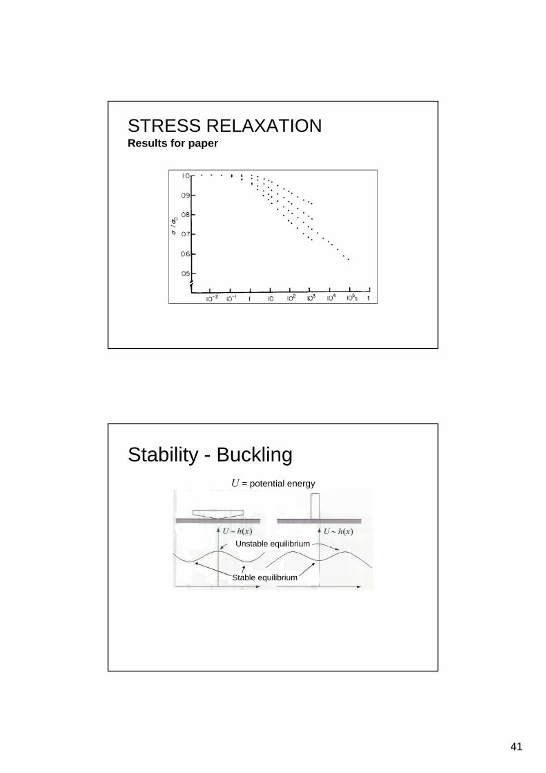
STRESS RELAXATIONResults for paper

Stability - BucklingU = potential energy

Unstable equilibrium

Stable equilibrium

42

Euler buckling of importance for compression testing

Plasticity and failure criteria under multi-axial loading conditions

Example: von Mises yield criterion for isotropic materials

1/ 22 2 2 2 2 23 3 3x y z x y x z y z xy xz zy Yσ σ σ σ σ σ σ σ σ τ τ τ σ⎡ ⎤+ + − − − + + + =⎣ ⎦

22 2σ σ τ σ σ⎛ ⎞

Example: Tsai-Wu’s failure criterion for an orthotropic material

1 1 1 1 1

L T LT L T

Lt Lc Tt Tc f Lt Lc Tt Tc

L TLt Lc Tt Tc

σ σ τ σ σσ σ σ σ τ σ σ σ σ

σ σσ σ σ σ

⎛ ⎞+ + − +⎜ ⎟⎜ ⎟

⎝ ⎠⎛ ⎞ ⎛ ⎞

+ + + =⎜ ⎟ ⎜ ⎟⎝ ⎠ ⎝ ⎠

43

After Lecture 5 you should be able to

• discuss the mechanical behaviour of particularly paper and paperboard packaging materials in terms of theand paperboard packaging materials in terms of the most important types of models used in solid mechanics.