Fundamentals of Radio Communications - Wiley...2 FUNDAMENTALS OF RADIO COMMUNICATIONS Low frequencies (LF) are frequencies from 30 kHz up to 3 MHz. In the 1950s and 1960s they were

CHAPTER ONE

Fundamentals of RadioCommunications

The purpose of this chapter is to familiarize the reader with the basic propagation

characteristics that describe various wireless communication channels, such as

terrestrial, atmospheric, and ionospheric for VHF to the X-band. Well-known

standards in wireless communication [1–10] are introduced for the prediction of path

losses and fading effects of any radio signal in various communication links, and

finally, new possibilities that can be obtained using smart antennas are discussed.

1.1. RADIO COMMUNICATION LINK

Different radio communication links (land, land-to-air, air-to-air) covering different

atmospheric and ionospheric conditions, include several components having a

plethora of physical principles and processes, with their own independent or

correlated working characteristics and operating elements. A simple scheme of such

a radio communication link consists of a transmitter (T), a receiver (R), and a

propagation channel. The main output characteristics of such a link depend on the

conditions of radio propagation in different kinds of environments, as shown in

Figure 1.1. According to Reference [6], there are three main independent electronic

and electromagnetic design tasks related to this wireless communication network.

The first task is the transmitter antenna operation including the specification of the

electronic equipment that controls all operations within the transmitter. The second

task is to understand, model, and analyze the propagation properties of the channel

that connects the transmitting and receiving antennas. The third task concerns the

study of all operations related to the receiver.

Radio Propagation and Adaptive Antennas for Wireless Communication Links: Terrestrial, Atmosphericand Ionospheric, by Nathan Blaunstein and Christos ChristodoulouCopyright # 2007 John Wiley & Sons, Inc.

1

The propagation channel is influenced by the various obstructions surrounding

antennas and the existing environmental conditions. Another important question for

a personal receiver (or handheld) antenna is also the influence of the human body on

the operating characteristics of the working antenna. The various blocks that

comprise a propagation channel are shown in Figure 1.1.

Its main output characteristics depend on the conditions of radio wave

propagation in the various operational environments where such wireless

communication links are used. Next, we briefly describe the frequency spectrum,

used in terrestrial, atmospheric, and ionospheric communications, and we classify

some common parameters and characteristics of a radio signal, such as its path loss

and fading for various situations, which occur in practice.

1.2. FREQUENCY BAND FOR RADIO COMMUNICATIONS

The frequency band is a main characteristic for predicting the effectiveness of

radio communication links that we consider here. The optimal frequency band

for each propagation channel is determined and limited by the technical re-

quirements of each communication system and by the conditions of radio

propagation through each channel. First, consider the spectrum of radio frequencies

and their practical use in various communication channels [1–5].

Extremely low and very low frequencies (ELF and VLF) are frequencies below

3 kHz and from 3 kHz to 30 kHz, respectively. The VLF band corresponds to waves,

which propagate through the wave guide formed by the Earth’s surface and the

ionosphere at long distances with a low degree of attenuation (0.1–0.5 per 1000 km

[1–5]).

Wireless Propagation ChannelWireless Propagation Channel

ReceiverTransmitter

ElectronicChannel

Electronic

Channel

Additivenoise

AbsorptionAttenuation(path loss)

Multiplicativenoise

(fading)

Additivenoise

Propagation Channel

FIGURE 1.1. A wireless communication link scheme.

2 FUNDAMENTALS OF RADIO COMMUNICATIONS

Low frequencies (LF) are frequencies from 30 kHz up to 3 MHz. In the 1950s and

1960s they were used for radio communication with ships and aircraft, but since then

they are used mainly with broadcasting stations. Because such radio waves

propagate along the ground surface, they are called ‘‘surface’’ waves [1–5].

High frequencies (HF) are those that are located in the band from 3 MHz up to

30 MHz. Signals in this spectrum propagate by means of reflections caused by the

ionospheric layers and are used for communication with aircraft and satellites, and

for long-distance land communication using broadcasting stations.

Very high frequencies (VHF) are located in the band from 30 MHz up to

300 MHz. They are usually used for TV communication, in long-range radar

systems and radio navigation systems.

Ultra high frequencies (UHF) are those that are located in the band from

300 MHz up to 3 GHz. This frequency band is very effective for wireless microwave

links, constructions of cellular systems (fixed and mobile), mobile–satellite

communication channels, medium range radars, and other applications.

In recent decades, radio waves with frequencies higher than 3 GHz (C, X,

K-bands, up to several hundred gigahertz, which in the literature are referred to as

microwaves) have begun to be widely used for constructing and performing modern

wireless communication channels.

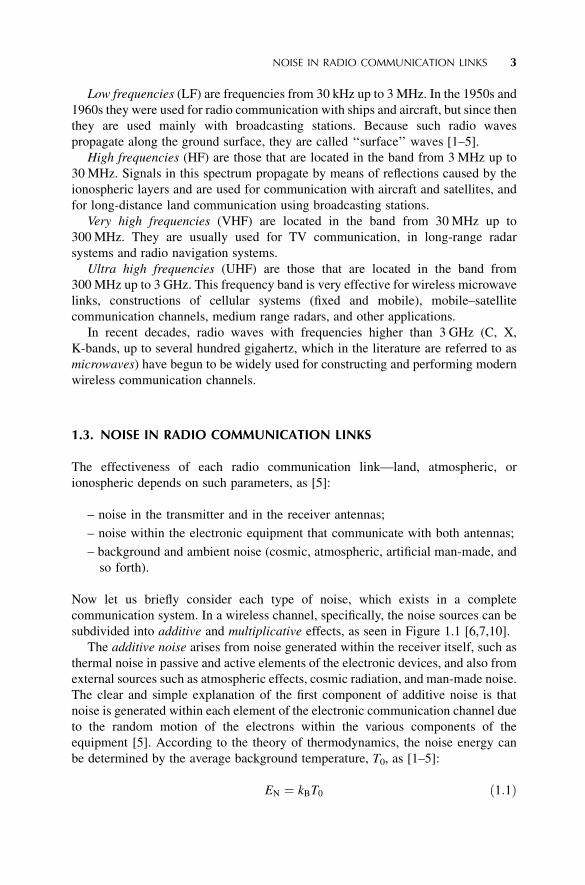
1.3. NOISE IN RADIO COMMUNICATION LINKS

The effectiveness of each radio communication link—land, atmospheric, or

ionospheric depends on such parameters, as [5]:

– noise in the transmitter and in the receiver antennas;

– noise within the electronic equipment that communicate with both antennas;

– background and ambient noise (cosmic, atmospheric, artificial man-made, and

so forth).

Now let us briefly consider each type of noise, which exists in a complete

communication system. In a wireless channel, specifically, the noise sources can be

subdivided into additive and multiplicative effects, as seen in Figure 1.1 [6,7,10].

The additive noise arises from noise generated within the receiver itself, such as

thermal noise in passive and active elements of the electronic devices, and also from

external sources such as atmospheric effects, cosmic radiation, and man-made noise.

The clear and simple explanation of the first component of additive noise is that

noise is generated within each element of the electronic communication channel due

to the random motion of the electrons within the various components of the

equipment [5]. According to the theory of thermodynamics, the noise energy can

be determined by the average background temperature, T0, as [1–5]:

EN ¼ kBT0 ð1:1Þ

NOISE IN RADIO COMMUNICATION LINKS 3

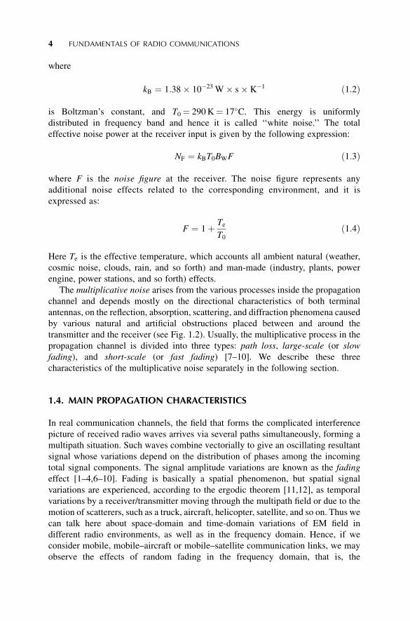
where

kB ¼ 1:38� 10�23 W� s� K�1 ð1:2Þ

is Boltzman’s constant, and T0¼ 290 K¼ 17�C. This energy is uniformly

distributed in frequency band and hence it is called ‘‘white noise.’’ The total

effective noise power at the receiver input is given by the following expression:

NF ¼ kBT0BWF ð1:3Þ

where F is the noise figure at the receiver. The noise figure represents any

additional noise effects related to the corresponding environment, and it is

expressed as:

F ¼ 1þ Te

T0

ð1:4Þ

Here Te is the effective temperature, which accounts all ambient natural (weather,

cosmic noise, clouds, rain, and so forth) and man-made (industry, plants, power

engine, power stations, and so forth) effects.

The multiplicative noise arises from the various processes inside the propagation

channel and depends mostly on the directional characteristics of both terminal

antennas, on the reflection, absorption, scattering, and diffraction phenomena caused

by various natural and artificial obstructions placed between and around the

transmitter and the receiver (see Fig. 1.2). Usually, the multiplicative process in the

propagation channel is divided into three types: path loss, large-scale (or slow

fading), and short-scale (or fast fading) [7–10]. We describe these three

characteristics of the multiplicative noise separately in the following section.

1.4. MAIN PROPAGATION CHARACTERISTICS

In real communication channels, the field that forms the complicated interference

picture of received radio waves arrives via several paths simultaneously, forming a

multipath situation. Such waves combine vectorially to give an oscillating resultant

signal whose variations depend on the distribution of phases among the incoming

total signal components. The signal amplitude variations are known as the fading

effect [1–4,6–10]. Fading is basically a spatial phenomenon, but spatial signal

variations are experienced, according to the ergodic theorem [11,12], as temporal

variations by a receiver/transmitter moving through the multipath field or due to the

motion of scatterers, such as a truck, aircraft, helicopter, satellite, and so on. Thus we

can talk here about space-domain and time-domain variations of EM field in

different radio environments, as well as in the frequency domain. Hence, if we

consider mobile, mobile–aircraft or mobile–satellite communication links, we may

observe the effects of random fading in the frequency domain, that is, the


complicated interference picture of the received signal caused by receiver/

transmitter movements, which is defined as the ‘‘Doppler shift’’ effect [1–7,10].

Numerous theoretical and experimental investigations in such conditions have

shown that the spatial and temporal variations of signal level have a triple nature

[1–7,10]. The first one is the path loss, which can be defined as a large-scale smooth

decrease in signal strength with distance between two terminals, mainly the

transmitter and the receiver. The physical processes that cause these phenomena are

the spreading of electromagnetic waves radiated outward in space by the transmitter

antenna and the obstructing effects of any natural or man-made objects in the

vicinity of the antenna. The spatial and temporal variations of the signal path loss are

large and slow, respectively.

Large-scale (in the space domain) or slow (in the time domain) fading is the

second nature of signal variations and is caused by diffraction from the obstructions

Base station

Scattering

Mobile

Diffrac

tion

Diffraction+

Scattering

Reflection

LOS

Diffraction

Scattering

FIGURE 1.2. Multipath effects caused by various natural and artificial obstructions placed

between and around the transmitting and the receiving antennas.

MAIN PROPAGATION CHARACTERISTICS 5

placed along the radio link surrounding the terminal antennas. Sometimes this

fading phenomenon is called the shadowing effect [6,7,10].

During shadow fading, the signal’s slow random variations follow either a

Gaussian distribution or a lognormal distribution if the signal fading is expressed in

decibels. The spatial scale of these slow variations depends on the dimensions of the

obstructions, that is, from several to several tens of meters. The variations of the total

EM field describe its structure within the shadow zones and are called slow-fading

signals.

The third nature of signal variations is the short-scale (in the space domain) or

fast (in the time domain) signal variations, which are caused by the mutual

interference of the wave components in the multiray field. The characteristic scale of

such waves in the space domain varies from half-wavelength to three-wavelength.

Therefore, these signals are usually called fast-fading signals.

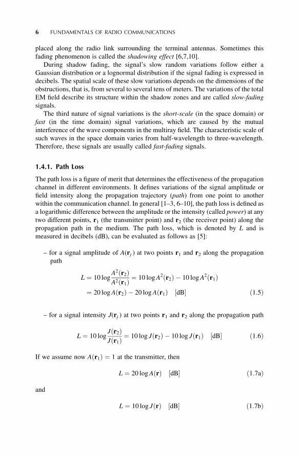
1.4.1. Path Loss

The path loss is a figure of merit that determines the effectiveness of the propagation

channel in different environments. It defines variations of the signal amplitude or

field intensity along the propagation trajectory (path) from one point to another

within the communication channel. In general [1–3, 6–10], the path loss is defined as

a logarithmic difference between the amplitude or the intensity (called power) at any

two different points, r1 (the transmitter point) and r2 (the receiver point) along the

propagation path in the medium. The path loss, which is denoted by L and is

measured in decibels (dB), can be evaluated as follows as [5]:

– for a signal amplitude of A(rj ) at two points r1 and r2 along the propagation

path

L ¼ 10 logA2ðr2ÞA2ðr1Þ

¼ 10 log A2ðr2Þ � 10 log A2ðr1Þ

¼ 20 log Aðr2Þ � 20 log Aðr1Þ ½dB ð1:5Þ

– for a signal intensity J(rj ) at two points r1 and r2 along the propagation path

L ¼ 10 logJðr2ÞJðr1Þ

¼ 10 log Jðr2Þ � 10 log Jðr1Þ ½dB ð1:6Þ

If we assume now Aðr1Þ ¼ 1 at the transmitter, then

L ¼ 20 log AðrÞ ½dB ð1:7aÞ

and

L ¼ 10 log JðrÞ ½dB ð1:7bÞ


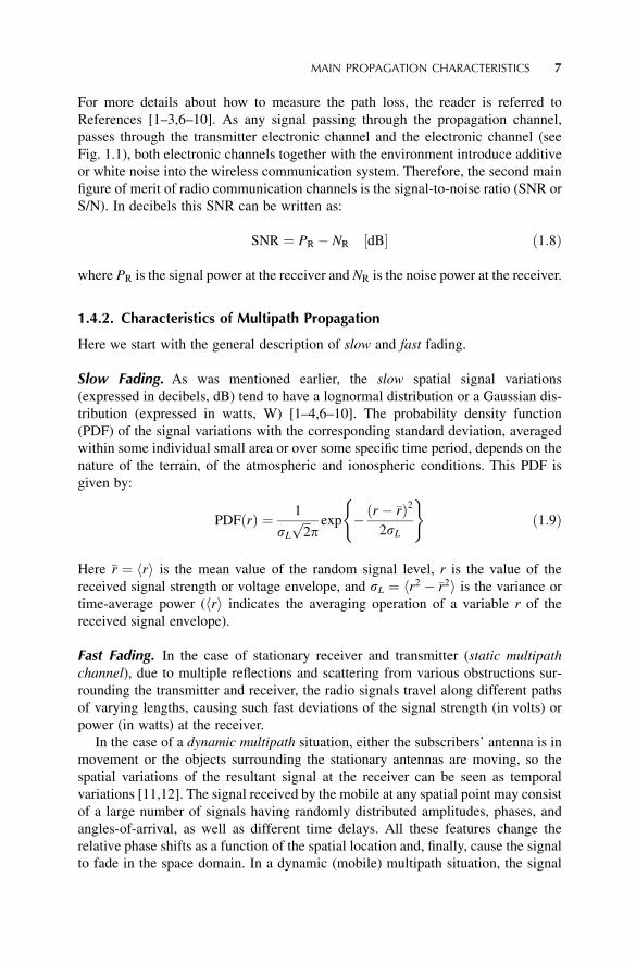
For more details about how to measure the path loss, the reader is referred to

References [1–3,6–10]. As any signal passing through the propagation channel,

passes through the transmitter electronic channel and the electronic channel (see

Fig. 1.1), both electronic channels together with the environment introduce additive

or white noise into the wireless communication system. Therefore, the second main

figure of merit of radio communication channels is the signal-to-noise ratio (SNR or

S/N). In decibels this SNR can be written as:

SNR ¼ PR � NR ½dB ð1:8Þ

where PR is the signal power at the receiver and NR is the noise power at the receiver.

1.4.2. Characteristics of Multipath Propagation

Here we start with the general description of slow and fast fading.

Slow Fading. As was mentioned earlier, the slow spatial signal variations

(expressed in decibels, dB) tend to have a lognormal distribution or a Gaussian dis-

tribution (expressed in watts, W) [1–4,6–10]. The probability density function

(PDF) of the signal variations with the corresponding standard deviation, averaged

within some individual small area or over some specific time period, depends on the

nature of the terrain, of the atmospheric and ionospheric conditions. This PDF is

given by:

PDFðrÞ ¼ 1

sL

ffiffiffi2p

pexp �ðr � �rÞ2

2sL

( )ð1:9Þ

Here �r ¼ hri is the mean value of the random signal level, r is the value of the

received signal strength or voltage envelope, and sL ¼ hr2 � �r2i is the variance or

time-average power (hri indicates the averaging operation of a variable r of the

received signal envelope).

Fast Fading. In the case of stationary receiver and transmitter (static multipath

channel), due to multiple reflections and scattering from various obstructions sur-

rounding the transmitter and receiver, the radio signals travel along different paths

of varying lengths, causing such fast deviations of the signal strength (in volts) or

power (in watts) at the receiver.

In the case of a dynamic multipath situation, either the subscribers’ antenna is in

movement or the objects surrounding the stationary antennas are moving, so the

spatial variations of the resultant signal at the receiver can be seen as temporal

variations [11,12]. The signal received by the mobile at any spatial point may consist

of a large number of signals having randomly distributed amplitudes, phases, and

angles-of-arrival, as well as different time delays. All these features change the

relative phase shifts as a function of the spatial location and, finally, cause the signal

to fade in the space domain. In a dynamic (mobile) multipath situation, the signal


fading at the mobile receiver occurs in the time domain. This temporal fading is

associated with a shift of frequency radiated by the stationary transmitter. In fact, the

time variations, or dynamic changes of the propagation path lengths, are related to

the Doppler effect, which is due to relative movements between a stationary base

station (BS) and a moving subscriber (MS).

To illustrate the effects of phase change in the time domain due to the Doppler

frequency shift (called the Doppler effect [1–4,6–10]), let us consider a mobile

moving at a constant velocity v, along the path XY, as shown in Figure 1.3. The

difference in path lengths traveled by a signal from source S to the mobile at points X

and Y is �‘ ¼ ‘ cos y ¼ v� cos y, where �t is the time required for the moving

receiver to travel from point X to Y along the path, and y is the angle between the

mobile direction along XY and direction to the source at the current point Y, that is,

YS. The phase change of the resultant received signal due to the difference in path

lengths is therefore

�F ¼ kD‘ ¼ 2pl‘ cos y ¼ 2pvDt

lcos y ð1:10Þ

Hence the apparent change in frequency radiated, or Doppler shift, is given by fD,

where

fD ¼1

2p��

�t¼ v

lcos y ð1:11Þ

It is important to note from Figure 1.3 that the angles y for points X and Y are the

same only when the corresponding lines XS and YS are parallel. Hence, this figure is

correct only in the limit when the terminal S is far away from the moving antenna at

points X and Y. Many authors have ignored this fact during their geometrical

explanation of the Doppler effect [1–4,10]. Because the Doppler shift is related to

the mobile velocity and the spatial angle between the direction of mobile motion and

the direction of arrival of the signal, it can be positive or negative depending on

FIGURE 1.3. Geometry of the mobile link for Doppler effect estimation.


whether the mobile receiver is moving toward or away from the transmitter. In fact,

from Equation (1.11), if the mobile moves toward the direction of arrival of the

signal with radiated frequency fc, then the received frequency is increased, that is the

apparent frequency is fc þ fD. When the mobile moves away from the direction of

arrival of the signal then the received frequency is decreased, that is the apparent

frequency is fc � fD. The maximum Doppler shift is fDmax ¼ v=l, which, in our

futher description will simply be denoted as fm.

There are many probability distribution functions that can be used to describe the

fast fading effects, such as, Rayleigh, Suzuki, Rician, Gamma, Gamma–Gamma,

and so on. Because the Rician distribution is very general [1–4,10], as it includes

both line-of-sight (LOS) together with scattering and diffraction with non-LOS, we

briefly describe it in the following paragraph.

To estimate the contribution of each signal component, at the receiver, due to the

dominant (or LOS) and the secondary (or multipath), the Rician parameter K is

usually introduced, as a ratio between these components [1–4,10], that is,

K ¼ LOS� Component power

Multipath� Component powerð1:12Þ

The Rician PDF distribution of the signal strength or voltage envelope r can be

defined as [1–4,10]:

PDFðrÞ ¼ r

s2exp � r2 þ A2

2s2

� �I0

Ar

s2

� �; for A > 0; r 0 ð1:13Þ

where A denotes the peak strength or voltage of the dominant component envelope,

s is the standard deviation of signal envelope, and I0ð�Þ is the modified Bessel

function of the first kind and zero-order. According to definition (1.12), we can now

rewrite the parameter K, which was defined above as the ratio between the dominant

and the multipath component power. It is given by

K ¼ A2

2s2ð1:14Þ

Using (1.14), we can rewrite (1.13) as a function of K only, [1–3,10]:

PDFðxÞ ¼ r

s2exp � r2

2s2

� �expð�KÞI0

r

s

ffiffiffi2p

K�

ð1:15Þ

For K ¼ 0, expð�KÞ ¼ 1 and I0ð0Þ ¼ 1, that is, the worst case of the fading channel.

The Rayleigh PDF, when there is no LOS signal and is equal to:

PDFðxÞ ¼ r

s2exp � r2

2s2

� �ð1:16Þ


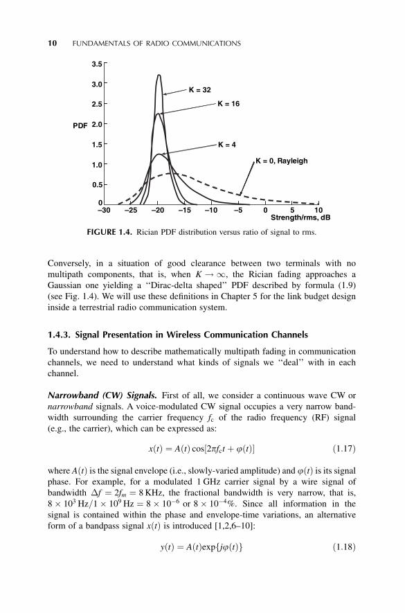
Conversely, in a situation of good clearance between two terminals with no

multipath components, that is, when K !1, the Rician fading approaches a

Gaussian one yielding a ‘‘Dirac-delta shaped’’ PDF described by formula (1.9)

(see Fig. 1.4). We will use these definitions in Chapter 5 for the link budget design

inside a terrestrial radio communication system.

1.4.3. Signal Presentation in Wireless Communication Channels

To understand how to describe mathematically multipath fading in communication

channels, we need to understand what kinds of signals we ‘‘deal’’ with in each

channel.

Narrowband (CW) Signals. First of all, we consider a continuous wave CW or

narrowband signals. A voice-modulated CW signal occupies a very narrow band-

width surrounding the carrier frequency fc of the radio frequency (RF) signal

(e.g., the carrier), which can be expressed as:

xðtÞ ¼ AðtÞ cos 2pfct þ jðtÞ½ ð1:17Þ

where AðtÞ is the signal envelope (i.e., slowly-varied amplitude) and jðtÞ is its signal

phase. For example, for a modulated 1 GHz carrier signal by a wire signal of

bandwidth �f ¼ 2fm ¼ 8 KHz, the fractional bandwidth is very narrow, that is,

8� 103 Hz=1� 109 Hz ¼ 8� 10�6 or 8� 10�4%. Since all information in the

signal is contained within the phase and envelope-time variations, an alternative

form of a bandpass signal xðtÞ is introduced [1,2,6–10]:

yðtÞ ¼ AðtÞexp jjðtÞf g ð1:18Þ

0.5

1.0

1.5

2.0

2.5

3.0

3.5

–15 –10 5 10

K = 16

K = 32

K = 4

K = 0, Rayleigh

0–30 –25 0

Strength/rms, dB–20 –5

PDF

FIGURE 1.4. Rician PDF distribution versus ratio of signal to rms.


which is also called the complex baseband representation of xðtÞ. By comparing

(1.17) and (1.18), we can see that the relation between the bandpass (RF) and the

complex baseband signals are related by:

xðtÞ ¼ Re yðtÞexp j2pfctð Þ½ ð1:19Þ

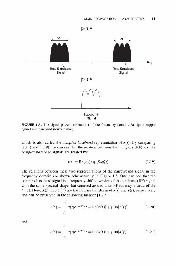
The relations between these two representations of the narrowband signal in the

frequency domain are shown schematically in Figure 1.5. One can see that the

complex baseband signal is a frequency shifted version of the bandpass (RF) signal

with the same spectral shape, but centered around a zero-frequency instead of the

fc [7]. Here, Xðf Þ and Yð f Þ are the Fourier transform of xðtÞ and yðtÞ, respectively

and can be presented in the following manner [1,2]:

Yðf Þ ¼ð1�1

yðtÞe�j2pftdt ¼ Re Yðf Þ½ þ j Im Yðf Þ½ ð1:20Þ

and

Xðf Þ ¼ð1�1

xðtÞe�j2pftdt ¼ Re Xðf Þ½ þ j Im Xðf Þ½ ð1:21Þ

BasebandSignal

f0

X(f)

Y(f)

∆f∆f

–fc +fc0 f

Real BandpassSignal

Real BandpassSignal

FIGURE 1.5. The signal power presentation of the frequency domain. Bandpath (upper

figure) and baseband (lower figure).


Substituting for xðtÞ in integral (1.21) from (1.19) gives:

Xðf Þ ¼ð1�1

Re yðtÞe j2pfct� �

e�j2pftdt ð1:22Þ

Taking into account that the real part of any arbitrary complex variable w can be

presented as:

Re½w ¼ 1

2wþ w�½

where w� is the complex conjugate, we can rewrite (1.22) in the following form:

Xðf Þ ¼ 1

2

ð1�1

yðtÞe j2pfct þ y�ðtÞe�j2pfct� �

e�j2pftdt ð1:23Þ

After comparing expressions (1.20) and (1.23), we get

Xðf Þ ¼ 1

2Yðf � fcÞ þ Y�ð�f � fcÞ½ ð1:24Þ

In other words, the spectrum of the real bandpass signal xðtÞ can be represented by

real part of that for the complex baseband signal yðtÞ with a shift of �fc along the

frequency axis. It is clear that the baseband signal has its frequency content centered

around the ‘‘zero’’ frequency value.

Now we notice that the mean power of the baseband signal yðtÞ gives the same

result as the mean-square value of the real bandpass (RF) signal xðtÞ, that is,

hPyðtÞi ¼hjyðtÞj2i

2¼ hyðtÞy

�ðtÞi2

� PxðtÞh i ð1:25Þ

The complex envelope yðtÞ of the received narrowband signal can be expressed

according to (1.18), within the multipath wireless channel, as a sum of phases of N

baseband individual multiray components arriving at the receiver with their

corresponding time delay, ti; i ¼ 0; 1; 2; . . . ;N � 1 [6–10]

yðtÞ ¼XN�1

i¼0

uiðtÞ ¼XN�1

i¼0

AiðtÞ exp jjiðt; tiÞ½ ð1:26Þ

If we assume that during the subscriber movements through the local area of service,

the amplitude Ai time variations are small enough, whereas phases ji vary greatly


due to changes in propagation distance between the base station and desired

subscriber, then there are great random oscillations of the total signal yðtÞ at the

receiver during its movement over a small distance. Since yðtÞ is the phase sum in

(1.26) of the individual multipath components, the instantaneous phases of the

multipath components result in large fluctuations, that is, fast fading, in the CW

signal. The average received power for such a signal over a local area of service can

be presented according to References [1–3,6–10] as:

PCWh i �XN�1

i¼0

A2i

� �þ 2

XN�1

i¼0

Xi; j 6¼i

AiAj

� �cos ji � jj

� �� ð1:27Þ

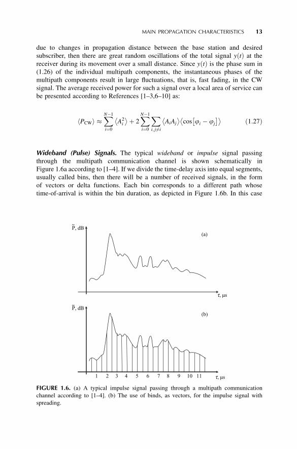
Wideband (Pulse) Signals. The typical wideband or impulse signal passing

through the multipath communication channel is shown schematically in

Figure 1.6a according to [1–4]. If we divide the time-delay axis into equal segments,

usually called bins, then there will be a number of received signals, in the form

of vectors or delta functions. Each bin corresponds to a different path whose

time-of-arrival is within the bin duration, as depicted in Figure 1.6b. In this case

1 2 3 4 5 6 7 8 9 10 11

(b)

t, µs

t, µs

P, dB

P, dB

(a)

~

~

FIGURE 1.6. (a) A typical impulse signal passing through a multipath communication

channel according to [1–4]. (b) The use of binds, as vectors, for the impulse signal with

spreading.


the time varying discrete-time impulse response can be expressed as:

hðt; tÞ ¼XN�1

i¼0

Aiðt; tÞexp �j2pfctiðtÞ½ d t� tiðtÞð Þ( )

exp �jjðt; tÞ½ ð1:28Þ

If the channel impulse response is assumed to be time invariant, or is at least

stationary over a short-time interval or over a small-scale displacement of the

receiver/transmitter, then the impulse response (1.28) reduces to

hðt; tÞ ¼XN�1

i¼0

AiðtÞ exp �jyi½ d t� tið Þ ð1:29Þ

where yi ¼ 2pfcti þ jðtÞ. If so, the received power delay profile for a wideband or

pulsed signal averaged over a small area can be presented simply as a sum of the

powers of the individual multipath components, where each component has a

random amplitude and phase at any time, that is,

Ppulse

� �¼

XN�1

i¼0

AiðtÞ exp �jyi½ j jf g2

* +�XN�1

i¼0

A2i

� �ð1:30Þ

The received power of the wideband or pulse signal does not fluctuate significantly

when the subscriber moves within a local area, because in practice, the amplitudes of

the individual multipath components do not change widely in a local area of service.

Comparison between small-scale presentations of the average power of the

narrowband (CW) and wideband (pulse) signals that is, (1.27) and (1.30), shows that

when hAiAji ¼ 0 or/and hcos½ji � jji ¼ 0, the average power for CW signal and

that for pulse are equivalent. This can occur when either the path amplitudes are

uncorrelated, that is, each multipath component is independent after multiple

reflections, diffractions, and scattering from obstructions surrounding both the

receiver and the transmitter or the base station and the subscriber antenna. It can also

occur when multipath phases are independently and uniformly distributed over the

range of b0; 2pc. This property is correct for UHF/X-waveband when the multipath

components traverse differential radio paths having hundreds of wavelengths

[6–10].

1.4.4. Parameters of the Multipath Communication Channel

So the question that is remains to be answered which kind of fading occurs in a given

wireless channel.

Time Dispersion Parameters. First some important parameters for a wideband

(pulse) signal passing through a wireless channel, can be determined, for a certain

threshold level X (in dB) of the channel under consideration, from the signal


power delay profile, such as mean excess delay, rms delay spread and excess delay

spread.

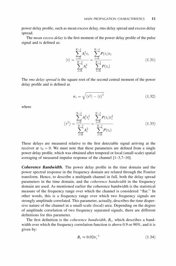
The mean excess delay is the first moment of the power delay profile of the pulse

signal and is defined as:

th i ¼

XN�1

i¼0

A2i ti

XN�1

i¼0

A2i

¼

XN�1

i¼0

PðtiÞti

XN�1

i¼0

PðtiÞð1:31Þ

The rms delay spread is the square root of the second central moment of the power

delay profile and is defined as

st ¼ffiffiffiffiffiffiffiffiffiffiffiffiffiffiffiffiffiffiffiffiffiffiht2i � hti2

qð1:32Þ

where

t2� �

¼

XN�1

i¼0

A2i t

2i

XN�1

i¼0

A2i

¼

XN�1

i¼0

PðtiÞt2i

XN�1

i¼0

PðtiÞð1:33Þ

These delays are measured relative to the first detectable signal arriving at the

receiver at t0 ¼ 0. We must note that these parameters are defined from a single

power delay profile, which was obtained after temporal or local (small-scale) spatial

averaging of measured impulse response of the channel [1–3,7–10].

Coherence Bandwidth. The power delay profile in the time domain and the

power spectral response in the frequency domain are related through the Fourier

transform. Hence, to describe a multipath channel in full, both the delay spread

parameters in the time domain, and the coherence bandwidth in the frequency

domain are used. As mentioned earlier the coherence bandwidth is the statistical

measure of the frequency range over which the channel is considered ‘‘flat.’’ In

other words, this is a frequency range over which two frequency signals are

strongly amplitude correlated. This parameter, actually, describes the time disper-

sive nature of the channel in a small-scale (local) area. Depending on the degree

of amplitude correlation of two frequency separated signals, there are different

definitions for this parameter.

The first definition is the coherence bandwidth, Bc, which describes a band-

width over which the frequency correlation function is above 0.9 or 90%, and it is

given by:

Bc � 0:02s�1t ð1:34Þ


The second definition is the coherence bandwidth, Bc, which describes a

bandwidth over which the frequency correlation function is above 0.5 or 50%, or:

Bc � 0:2s�1t ð1:35Þ

There is not any single exact relationship between coherence bandwidth and rms delay

spread, and equations (1.34) and (1.35) are only approximate equations [1–6,7–10].

Doppler Spread and Coherence Time. To obtain information about the time

varying nature of the channel caused by movements, from either the transmitter/

receiver or scatterers located around them, new parameters, such as the Doppler

spread and the coherence time, are usually introduced to describe the time variation

phenomena of the channel in a small-scale region. The Doppler spread BD is defined

as a range of frequencies over which the received Doppler spectrum is essentially

nonzero. It shows the spectral spreading caused by the time rate of change of the

mobile radio channel due to the relative motions of vehicles (and scatterers around

them) with respect to the base station. According to [1–4,7–10], the Doppler spread

BD depends on the Doppler shift fD and on the angle a between the direction of

motion of any vehicle and the direction of arrival of the reflected and/or scattered

waves (see Fig. 1.3). If we deal with the complex baseband signal presentation,

then we can introduce the following criterion: If the baseband signal bandwidth is

greater than the Doppler spread BD, the effects of Doppler shift are negligible at the

receiver.

Coherence time Tc is the time domain dual of Doppler spread, and it is used

to characterize the time varying nature of the frequency dispersiveness of the

channel in time coordinates. The relationship between these two-channel charac-

teristics is:

Tc �1

fm

¼ lv

ð1:36Þ

We can also define the coherence time according to [1–4,7–10] as the time duration

over which two multipath components of receiving signal have a strong potential for

amplitude correlation. One can also define the coherence time as the time over

which the correlation function of two various signals in the time domain is above 0.5

(or 50%). Then according to [7,10] we get

Tc �9

16pfm¼ 9l

16pv¼ 0:18

lv

ð1:37Þ

This definition is approximate and can be improved for modern digital

communication channels by combining Equations (1.36) and (1.37) as the geometric

mean between the two, this yields

Tc �0:423

fm¼ 0:423

lv

ð1:38Þ


The definition of coherence time implies that two signals arriving at the receiver

with a time separation greater than Tc are affected differently by the channel.

1.4.5. Types of Fading in Multipath Communication Channels

Let us now summarize the effects of fading, which may occur in static or dynamic

multipath communication channels.

Static Channel. In this case multipath fading is purely spatial and leads to con-

structive or destructive interference at various points in space, at any given instant

in time, depending on the relative phases of the arriving signals. Furthermore, fading

in the frequency domain does not change because the two antennas are stationary.

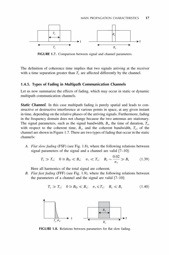
The signal parameters, such as the signal bandwidth, Bs, the time of duration, Ts,

with respect to the coherent time, Bc, and the coherent bandwidth, Tc, of the

channel are shown in Figure 1.7. There are two types of fading that occur in the static

channels:

A. Flat slow fading (FSF) (see Fig. 1.8), where the following relations between

signal parameters of the signal and a channel are valid [7–10]:

Tc � Ts; 0 ffi BD � Bs; st � Ts; Bc �0:02

st� Bs ð1:39Þ

Here all harmonics of the total signal are coherent.

B. Flat fast fading (FFF) (see Fig. 1.9), where the following relations between

the parameters of a channel and the signal are valid [7–10]:

Tc � Ts; 0 ffi BD � Bs; st4Ts; Bc � Bs ð1:40Þ

t f

sT

cT

cB

sB

FIGURE 1.7. Comparison between signal and channel parameters.

fcB

sB

sT ts t

FIGURE 1.8. Relations between parameters for flat slow fading.


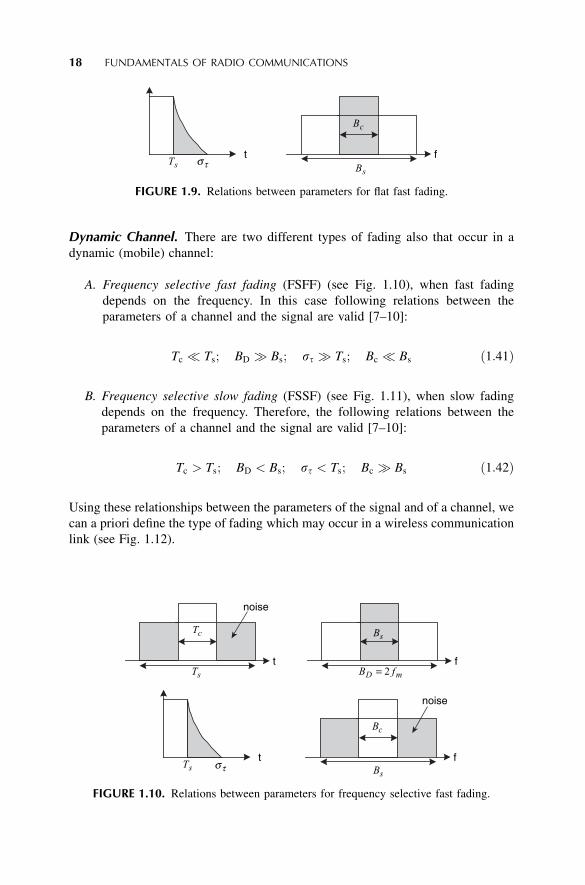
Dynamic Channel. There are two different types of fading also that occur in a

dynamic (mobile) channel:

A. Frequency selective fast fading (FSFF) (see Fig. 1.10), when fast fading

depends on the frequency. In this case following relations between the

parameters of a channel and the signal are valid [7–10]:

Tc � Ts; BD � Bs; st � Ts; Bc � Bs ð1:41Þ

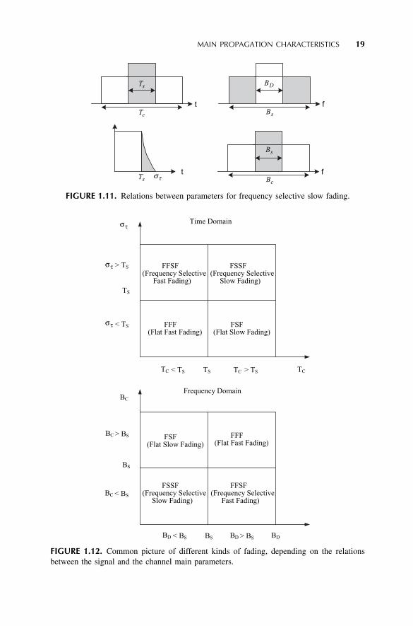
B. Frequency selective slow fading (FSSF) (see Fig. 1.11), when slow fading

depends on the frequency. Therefore, the following relations between the

parameters of a channel and the signal are valid [7–10]:

Tc > Ts; BD < Bs; st < Ts; Bc � Bs ð1:42Þ

Using these relationships between the parameters of the signal and of a channel, we

can a priori define the type of fading which may occur in a wireless communication

link (see Fig. 1.12).

f

sB

cB

sTt

ts

FIGURE 1.9. Relations between parameters for flat fast fading.

f

sB

mD fB 2=

sTt

tsT

cT

f

sB

cB

noise

noise

ts

FIGURE 1.10. Relations between parameters for frequency selective fast fading.


Time Domain

> TS

TS

< TS

FFSF(Frequency Selective

Fast Fading)

FSSF(Frequency Selective

Slow Fading)

FFF (Flat Fast Fading)

FSF (Flat Slow Fading)

TC < TS TS TC > TS TC

FFSF(Frequency Selective

Fast Fading)

FSSF(Frequency Selective

Slow Fading)

FFF (Flat Fast Fading)

FSF (Flat Slow Fading)

Frequency DomainBC

BC > BS

BS

BC < BS

BD < BS BS BD > BS BD

ts

ts

ts

FIGURE 1.12. Common picture of different kinds of fading, depending on the relations

between the signal and the channel main parameters.

sTt

f

DB

sBt

cT

sT

fcB

sB

ts

FIGURE 1.11. Relations between parameters for frequency selective slow fading.


1.5. PROBLEMS IN ADAPTIVE ANTENNAS APPLICATION

The main problem with land communication links is estimating the ratio between the

coherent and multipath components of the total signal. That is, the Ricean parameter

K, to predict the effects of multiplicative noise in the channel of each subscriber

located in different conditions in the terrestrial environment. This is shown in

Figure 1.13 for various subscribers numbered by i ¼ 1, 2, 3, . . . .

However, even a detailed prediction of the radio propagation situation for each

subscriber cannot completely resolve all issues of effective service and increase

quality of data stream sent to each user. For this purpose, in future generations of

wireless systems, adaptive or smart antenna systems are employed to reduce

interference and decrease bit error rate (BER). This topic will be covered in detail in

Chapter 8. We present schematically the concept of adaptive (smart) antennas in

Figure 1.14.

Building 1 Building 1

Building 1

House

Building 2House

House

Park

Tree

Tree FactoryTree

House

Shopping centre

House

K1K2

K3

K4

K5

K6

T

FIGURE 1.13. Scheme of various scenarios in urban communication channel.


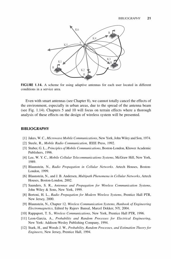
Even with smart antennas (see Chapter 8), we cannot totally cancel the effects of

the environment, especially in urban areas, due to the spread of the antenna beam

(see Fig. 1.14). Chapters 5 and 10 will focus on terrain effects where a thorough

analysis of these effects on the design of wireless system will be presented.

BIBLIOGRAPHY

[1] Jakes, W. C., Microwave Mobile Communications, New York, John Wiley and Son, 1974.

[2] Steele, R., Mobile Radio Communication, IEEE Press, 1992.

[3] Stuber, G. L., Principles of Mobile Communications, Boston-London, Kluwer Academic

Publishers, 1996.

[4] Lee, W. Y. C., Mobile Cellular Telecommunications Systems, McGraw Hill, New York,

1989.

[5] Blaunstein, N., Radio Propagation in Cellular Networks. Artech Houses, Boston-

London, 1999.

[6] Blaunstein, N., and J. B. Andersen, Multipath Phenomena in Cellular Networks, Artech

Houses, Boston-London, 2002.

[7] Saunders, S. R., Antennas and Propagation for Wireless Communication Systems,

John Wiley & Sons, New York, 1999.

[8] Bertoni, H. L., Radio Propagation for Modern Wireless Systems, Prentice Hall PTR,

New Jersey, 2000.

[9] Blaunstein, N., Chapter 12, Wireless Communication Systems, Hanbook of Engineering

Electromagnetics, Edited by Rajeev Bansal, Marcel Dekker, NY, 2004.

[10] Rappaport, T. S., Wireless Communications, New York, Prentice Hall PTR, 1996.

[11] Leon-Garcia, A., Probability and Random Processes for Electrical Engineering,

New York: Addison-Wesley Publishing Company, 1994.

[12] Stark, H., and Woods J. W., Probability, Random Processes, and Estimation Theory for

Engineers, New Jersey, Prentice Hall, 1994.

T

K1

K2

K3

K4

K5

K6

R

R

R

R

FIGURE 1.14. A scheme for using adaptive antennas for each user located in different

conditions in a service area.

BIBLIOGRAPHY 21

Documents

Fundamentals of Radio Communications - Wiley...2 FUNDAMENTALS OF RADIO COMMUNICATIONS Low frequencies (LF) are frequencies from 30 kHz up to 3 MHz. In the 1950s and 1960s they were