Fundamentals of Deployment - NCAEMSA · Fundamentals of Deployment ... •Unit hour utilization and the relevant variables ... •Demand analysis versus "waiting‐line analysis

Fundamentals of Deployment

Randy D. Kearns MSA, DHA(c), CEM

Clinical Instructor, Department of Surgery

University of North Carolina, School of Medicine

February 2009

W’s

• Who:

– Randy Kearns

• What

– Fundamentals of Deployment for EMS Systems

• Why

– Why is this important to me?

– New sense of urgency to be efficient .

Disclaimer

• UNC

– Researcher‐NC Burn Disaster Program

• NCOEMS

• ASPR

• FEMA (Reservist)

– Branch Director w/ Specialty: ES Branch

Who cares? Who is our audience?

• Public Safety Model

• Business Model

• Hospital Based Model

What do they want? and,

What do they need?

Overview

• System status management, dynamic versus static deployment (SSM)

• Call timeline gap analysis, event chain performance improvement, (patient) throughput measurements (ToT)– Time on task factors, choke points, etc.

• Unit hour utilization and the relevant variables (UHU)• Demand analysis versus "waiting‐line analysis/measurement"

(also referred to in the statistical world as Markov Chain)• Stand ready costs• Unit hour costs and how it relates to fees for service/costs for

services• Risk versus Utilization situations and relative costs• Measuring fixed costs versus variable costs

In a word, deployment is based on. . .

Utilization of

Positioning of

Cost of

Determining the need for

Definitions

• System Status Management

– The Strategy of Ambulance Placement

Deployment

• Static

– Examples

• Dynamic

– Examples

Static

• What influences selection for a base location?

– Data

– Availability of the land?

– Price of the land?

– Political influence?

– Do you redeploy ambulances when there is a call in an adjacent location?

Dynamic

• What data do you use?

• What time blocks do you move?

• How does staffing mirror demand?

• What process do you have in place to redeploy units?

Utilization of

Positioning of

Cost of


Time on Task (ToT)

• Pre‐call

• Call to 9‐1‐1 or similar answering point

• PAI and Dispatch (queue)

• Chute Time

• Response Time

• On scene Time

• Transport Time

• Arrival and ready for service

Response Times

• Average

• Fractal

• (probably best but both are acceptable)

Unit Hours – Unit Hour Utilization (UHU)

• 1 ambulance, 24 hours / day, 365 days/ year

• 1 x 24 x 365 = 8760 unit hours

• (17,520 worked hours)

• If there is one call per hour then there will be a utilization of 1.0 UHU 24/24 = 1.

• 2 calls per 24 hr shift = 0.083 UHU (2/24 = 0.083)


UHU Cont.







UHU Cont.

• Time on Task issues

• Choke Points

Utilization of

Positioning of

Cost of


Unit Hour Costs (Direct Costs)• 1 ambulance, 24 hours / day, 365 days/ year

• 1 x 24 x 365 = 8760 unit hours

• (17,520 worked hours)

• If the average hourly rate is $15.00 per hour, then the salary for the unit is $15.00 x 17,520 = $262,800.

• If the benefits represent 25%, then the benefit value is $65,700

• If the supplies represent 30% of the value of the employee costs then; $140,786

• If the mileage (vehicle component is 30% of the total) then the vehicle component is: $234,643

• $703,929 / 8760 = $80.36 (significantly short of total costs per unit hour)

Medicare Source – Calculating Costs– Components

• National Uniform Base Rate – NUBR

• Relative Value Unit – RVU

• Geographic Adjustment Factor (GAF [GPCI])

• Loaded Mileage – LM

• Mileage Rate – MR

• Point of Pick up modification – POP

• Additional Payments for certain specified periods

– (NUBR x RVU x 0.7 x GAF) + (NUBR x RVU x 0.3) = Xb

– (LM x MR x POP) = Xm

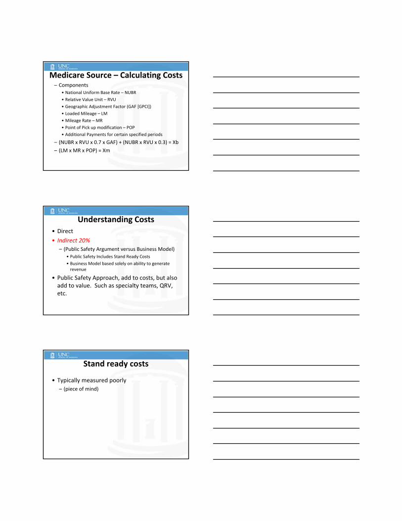
Understanding Costs• Direct

• Indirect 20%

– (Public Safety Argument versus Business Model)

• Public Safety Includes Stand Ready Costs

• Business Model based solely on ability to generate revenue

• Public Safety Approach, add to costs, but also add to value. Such as specialty teams, QRV, etc.

Stand ready costs

• Typically measured poorly

– (piece of mind)

Risk and Service Availability

• How do you place resources when the services are seldom utilized?

QRV

QRV


Utilization of

Positioning of

Cost of

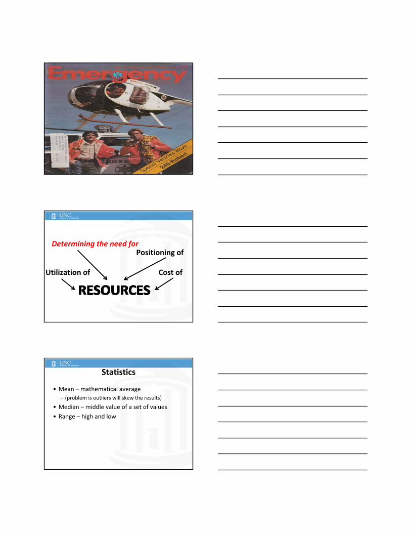
Statistics

• Mean – mathematical average

– (problem is outliers will skew the results)

• Median – middle value of a set of values

• Range – high and low

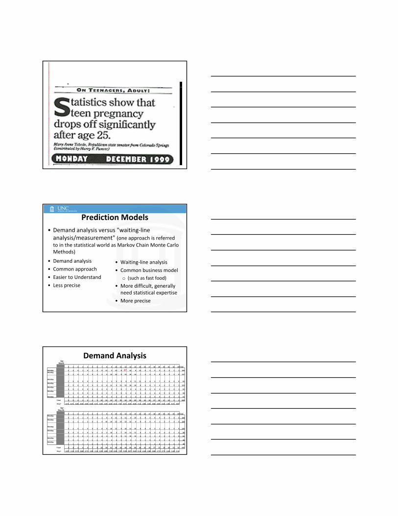
Prediction Models

• Demand analysis versus "waiting‐line analysis/measurement" (one approach is referred to in the statistical world as Markov Chain Monte Carlo Methods)

• Demand analysis

• Common approach

• Easier to Understand

• Less precise

• Waiting‐line analysis

• Common business model

o (such as fast food)

• More difficult, generally need statistical expertise

• More precise

Demand AnalysisApr-

May05

0 1 2 3 4 5 6 7 8 9 10 11 12 13 14 15 16 17 18 19 20 21 22 23Total

Monday 1 2 0 1 0 1 2 6 11 3 13 8 17 12 9 13 6 5 5 5 2 2 1 1 126Monday

0 1 0 2 0 0 0 2 6 12 12 8 10 16 14 7 4 4 0 8 6 3 2 0 117

Monday1 0 0 0 0 1 0 1 1 3 9 8 8 9 11 11 3 4 2 7 3 0 0 0 82

Monday2 0 0 0 0 0 3 2 6 11 9 11 10 16 16 8 5 6 3 5 2 7 0 1 123

Monday0 0 1 0 0 0 0 2 5 8 7 8 7 9 6 5 8 2 6 3 3 1 0 1 82

Monday1 1 0 0 0 0 0 2 0 7 5 8 5 3 5 4 5 1 6 5 0 0 0 0 58

Monday 0 1 1 0 0 0 0 9 2 0 2 2 4 1 4 2 3 2 5 9 1 0 2 1 51

Total 5 5 2 3 0 2 5 24 31 44 57 53 61 66 65 50 34 24 27 42 17 13 5 4 639

Avg # 0.71 0.71 0.29 0.43 0.00 0.29 0.71 3.43 4.43 6.29 8.14 7.57 8.71 9.43 9.29 7.14 4.86 3.43 3.86 6.00 2.43 1.86 0.71 0.57

Apr-May-06

0 1 2 3 4 5 6 7 8 9 10 11 12 13 14 15 16 17 18 19 20 21 22 23TotalMonday

0 1 0 1 0 0 0 1 6 8 11 9 11 8 14 5 8 3 6 4 5 3 2 2 108Monday

2 1 1 1 3 2 1 4 10 10 13 14 12 12 9 8 5 2 4 1 2 7 3 2 129

Monday0 1 0 1 0 0 3 8 9 10 13 9 16 11 10 8 8 8 3 1 2 2 2 5 130

Monday0 0 2 1 0 2 1 3 2 10 3 7 10 11 11 6 3 5 3 0 4 3 1 2 90

1 1 0 0 1 0 2 4 4 8 9 8 11 10 12 6 4 1 3 2 2 2 0 0 91Monday

0 3 1 1 0 1 1 0 1 4 4 3 2 3 7 2 1 0 4 0 3 3 2 3 49Monday

1 1 1 1 1 2 0 3 2 1 3 3 3 5 3 1 2 1 4 4 1 4 0 1 48

Total 4 8 5 6 5 7 8 23 34 51 56 53 65 60 66 36 31 20 27 12 19 24 10 15 645

Avg # 0.57 1.14 0.71 0.86 0.71 1.00 1.14 3.29 4.86 7.29 8.00 7.57 9.29 8.57 9.43 5.14 4.43 2.86 3.86 1.71 2.71 3.43 1.43 2.14

0.571.140.710.860.711.001.143.294.867.298.007.579.298.579.435.144.432.863.861.712.713.431.432.14

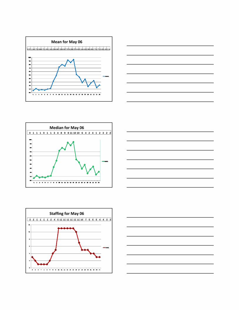
Mean for May 06

0 1 1 1 0 1 1 3 4 8 9 8 11 10 10 6 4 2 4 1 2 3 2 2

Median for May 06

3 2 1 1 1 1 2 4 5 11 11 11 11 11 11 10 7 5 5 5 4 4 3 3

Staffing for May 06

0.61.10.70.90.71.01.13.34.97.38.07.69.38.69.45.14.42.93.91.72.73.41.42.10 1 1 1 0 1 1 3 4 8 9 8 11 10 10 6 4 2 4 1 2 3 2 23 2 1 1 1 1 2 4 5 11 11 11 11 11 11 10 7 5 5 5 4 4 3 3

Demand Analysis for May 06, Staffing vs. Mean and Median Data

Predicting Demand

• Demand analysis versus "waiting‐line analysis/measurement" (also referred to in the statistical world as Markov Chains)

Typical View• Resources = Supply

– (From the Economics Model; Supply vs. Demand)

– (Influencing factors; Price, Marketing, Quantity)

Waiting Line Analysis

• Queue

– A single waiting line

• (order in which customers are served)

• Waiting line system consists of:

– Arrivals

– Servers

– Waiting line structures

Waiting Line Analysis components:

• Calling Population

• Arrival rate

– (must be less than service rate or system never clears out)

• Service time

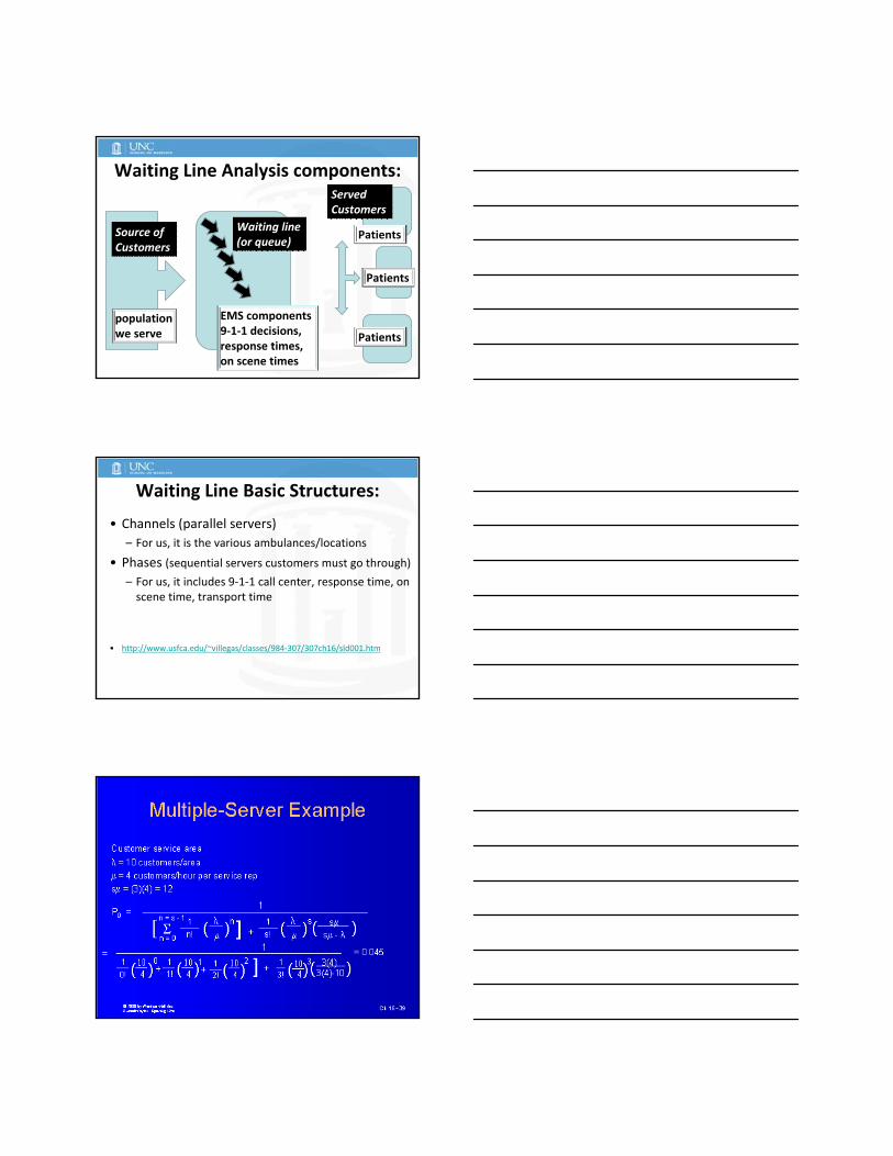
Waiting Line Analysis components:

Source of Customers

Source of Customers

population we serve

Waiting line (or queue)

Waiting line (or queue)

Served Customers

Served Customers

EMS components9‐1‐1 decisions, response times, on scene times

Patients

Patients

Patients

Waiting Line Basic Structures:

• Channels (parallel servers)

– For us, it is the various ambulances/locations

• Phases (sequential servers customers must go through)

– For us, it includes 9‐1‐1 call center, response time, on scene time, transport time

• http://www.usfca.edu/~villegas/classes/984‐307/307ch16/sld001.htm

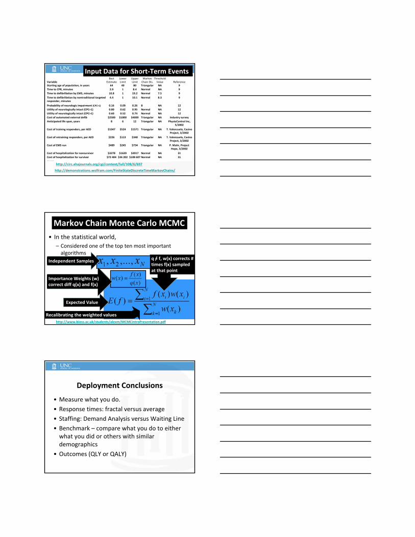
http://demonstrations.wolfram.com/FiniteStateDiscreteTimeMarkovChains/

http://circ.ahajournals.org/cgi/content/full/108/6/697

Variable Best

Estimate Lower Limit

Upper Limit

Markov Chain Dis.

Threshold Value Reference

Starting age of population, in years 64 40 80 Triangular NA 9

Time to CPR, minutes 2.9 1 8.4 Normal NA 9

Time to defibrillation by EMS, minutes 10.8 1 19.2 Normal 7.5 9

Time to defibrillation by nontraditional targeted responder, minutes

4.4 1 10.1 Normal 8.3 9

Probability of neurologic impairment (CPC>1) 0.16 0.09 0.26 B NA 12

Utility of neurologically intact (CPC=1) 0.80 0.62 0.95 Normal NA 12

Utility of neurologically intact (CPC>1) 0.60 0.52 0.74 Normal NA 12

Cost of automated external defib $2500 $1000 $4000 Triangular NA Industry survey

Anticipated life span, years 8 6 12 Triangular NA PhysioControl Inc, 5/2002

Cost of training responders, per AED $1047 $524 $1571 Triangular NA T. Valenzuela, Casino Project, 3/2002

Cost of retraining responders, per AED $226 $113 $340 Triangular NA T. Valenzuela, Casino Project, 3/2002

Cost of EMS run $489 $245 $734 Triangular NA P. Mohr, Project Hope, 3/2002

Cost of hospitalization for nonsurvivor $3278 $1639 $4917 Normal NA 31

Cost of hospitalization for survivor $72 404 $36 202 $108 607 Normal NA 31NA indicates not applicable.

Input Data for Short‐Term Events

• In the statistical world,

– Considered one of the top ten most important algorithms

http://www.bioss.ac.uk/students/alexm/MCMCintroPresentation.pdf

Markov Chain Monte Carlo MCMC

Expected Value

q = f, w(x) corrects # times f(x) sampled at that point

Recalibrating the weighted values

Expected ValueIndependent Samples /

Importance Weights (w) correct diff q(x) and f(x)

Deployment Conclusions

• Measure what you do.

• Response times: fractal versus average

• Staffing: Demand Analysis versus Waiting Line

• Benchmark – compare what you do to either what you did or others with similar demographics

• Outcomes (QLY or QALY)

Deployment Conclusions – cont.

• Have a plan, follow the plan.

• Process to hold calls or surge capacity to meet demand?

• How do we see ourselves?

• How do others see us?

Questions?

• 101‐87

• UNC over Duke

Documents

Fundamentals of Deployment - NCAEMSA · Fundamentals of Deployment ... •Unit hour utilization and the relevant variables ... •Demand analysis versus "waiting‐line analysis