Embed Size (px)
Citation preview

Fundamentals of Computer Design
Rapid Pace of Development
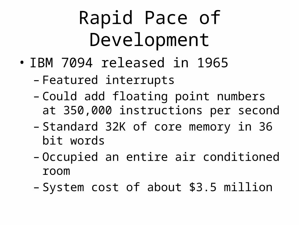
• IBM 7094 released in 1965– Featured interrupts– Could add floating point numbers at 350,000
instructions per second– Standard 32K of core memory in 36 bit words– Occupied an entire air conditioned room– System cost of about $3.5 million

This laptop
• Fujitsu Lifebook T4220 purchased in 2008– 16 GFLOPS (we’ll see later this is not a particularly
good benchmark)– Standard 2GB of core memory in 64 bit words– Occupies 12” by 9” by 1.5” space– System cost of about $2,000

• Transistors per inch square– Twice as many after ~1.5-2 years
• Related trends– Processor performance
Twice as fast after ~18 months– Memory capacity
Twice as much in <2 years• Not a true law but an observation
– We’re getting close to hitting the physical limits
Moore’s Law

The Shrinking Chip
• Human Hair: 100 microns wide– 1 micron is 1 millionth of a meter
• Bacterium: 5 microns• Virus: 0.8 microns• Early microprocessors: 10-15 micron
technology• 1997: 0.35 Micron• 1998: 0.25 Micron• 1999: 0.18 Micron• 2001: 0.13 Micron• 2003: 0.09 Micron• 2007: 0.065 Micron• 2009: 0.045 Micron• Physical limits believed to be around
0.016 Microns, should reach it around 2018

6
Size
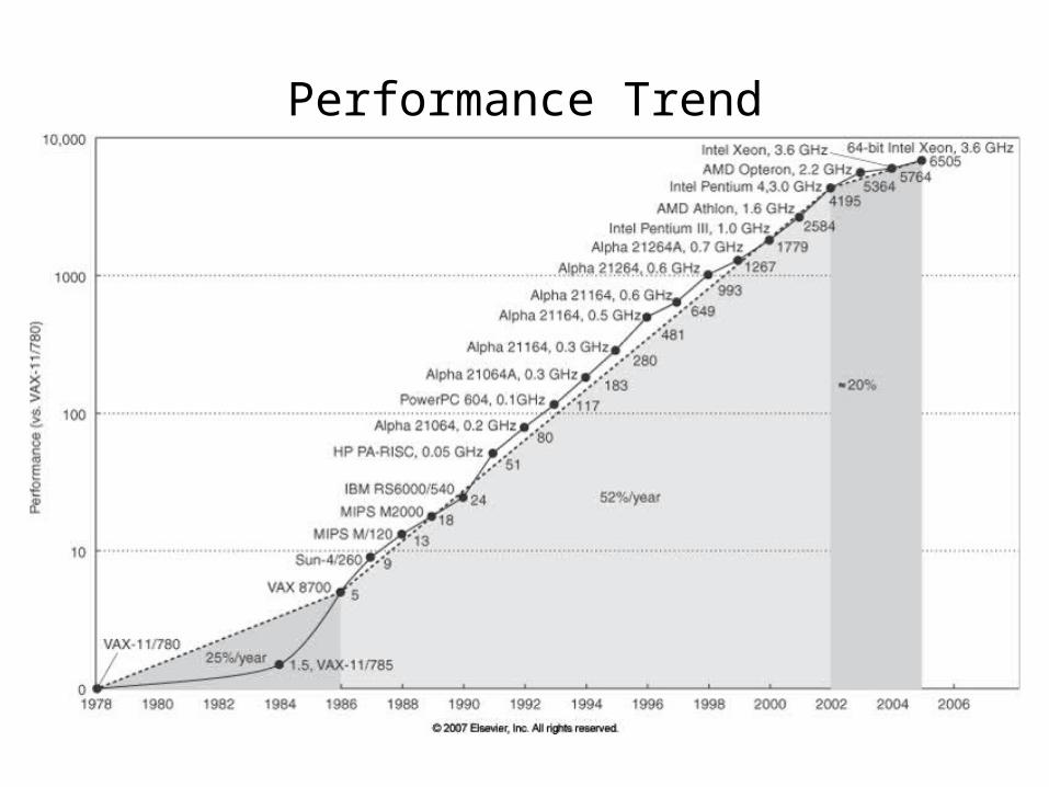
Performance Trend

RISC vs. CISC
• Big debate in the 80’s• Ideas from RISC won
– Although you don’t think of it as RISC, today’s Intel Architecture adopted many RISC ideas internally

Terms for a Computer Designer
• Instruction Set Architecture – The assembly instructions visible to a programmer
• Organization – Mostly transparent to the programmer, but high-level design aspects such as how much cache, replacement policies, cache mapping algorithm, bus structure, internal CPU design.
• Computer Architecture – We’ll refer to this as instruction set design, organization of the hardware design, and the actual hardware itself.

ISA for this class
• Mostly a MIPS-like ISA– 32 general purpose and 32 floating point registers– Load-store architecture
• Memory Addressing– Byte addressing– Objects in MIPS must be byte aligned
• Addressing Modes– Register, Immediate, Displacement

ISA for this class
• Types and sizes of operands– 8-bit ASCII to 64 it double precision
• Operations– Data transfer, arithmetic, logical, control, floating
point• Control Flow instructions• Encoding on an ISA
– Fixed length vs. Variable length

Other Design Factors
Power, Cooling, Logic, Fabrication
CPU, Memory, Interconnect, Buses
Operating System, Programming Lang
Instruction Set Architecture
Utilities, User Applications
Market Forces

Conflicting Requirements
• To minimize cost implies a simple design• To maximize performance implies complex
design or sophisticated technology• Time to market matters! Implies simple design
and great secrecy• Time to productivity! Implies need complete
vertical solutions in place• Don’t mess up – requires simulation, QA,
quantification

Technology Trends
• In 1943, Thomas Watson predicted “I think there is a world market for maybe five computers." – (The IBM PC was an “undercover” project and
saved the company)• In the 70’s and 80’s IBM pursued the high-
speed Josephson Junction, spending $2 billion, before scrapping it and using CMOS like everyone else.

Current Trends
• Memory use by programs growing by a factor of 1.5 to 2 per year. – Lesson: don’t make your word size or address space too small!
• Replacement of assembly by HLL’s– Lesson: compilers are critical!
• Growing demand on multimedia– Lesson: Design for high-speed graphic interfaces.
• Growing demand for networking. – Lesson: Also design for high-speed I/O
• Growing demand for simplicity in attaching I/O devices– Lesson: Rise of USB, perhaps Firewire next?
• Growing demand for mobile computing– Lesson: Need ability to adapt to low power scenarios
Implementation Trends
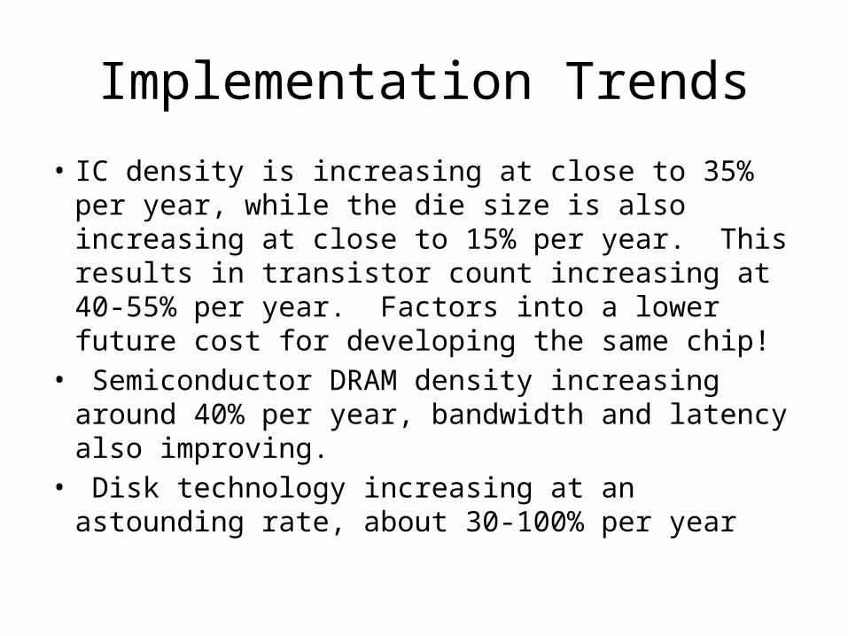
• IC density is increasing at close to 35% per year, while the die size is also increasing at close to 15% per year. This results in transistor count increasing at 40-55% per year. Factors into a lower future cost for developing the same chip!
• Semiconductor DRAM density increasing around 40% per year, bandwidth and latency also improving.
• Disk technology increasing at an astounding rate, about 30-100% per year

PC Hard Drive Capacity

Bandwidth vs. Latency

Chip Production• Ingot of purified silicon – 1 meter
long, sliced into thin wafers• Chips are etched – much like
photography– UV light through multiple masks– Circuits laid down through mask
• Process takes about 3 months
View ofCross-Section

Yield
13/16 working chips81.25% yield
1/4 working chips25.0% yield
ManufacturingDefects
Size Matters! (of the die, anyway)
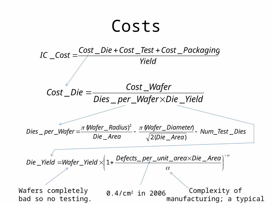
Costs
Yield
PackagingCostTestCostDieCostCostIC
____
YieldDieWaferperDies
WaferCostDieCost
___
__
DiesTestNumAreaDie
DiameterWafer
AreaDie
RadiusWaferWaferperDies __
)_(2
)_(
_
)_(__
2
AreaDieareaunitperDefects
YieldWaferYieldDie____
1__
Complexity of manufacturing; a typical a = 4
Wafers completely bad so no testing. Assume 100%
0.4/cm2 in 2006

Some Sizes• 0.25u Pentium II = 105 mm2
• 0.25u PPC 604e = 47.3 mm2
• 0.18u Pentium 4: 217 mm2
• 0.18u Transmeta TM5600 88 mm2
• 0.90u VIA C7M 30mm2
• 0.065u Athlon X2 (Brisbane) 118 mm2
• 0.065u Core 2 Due (Conroe) 143 mm2
• 0.045u Atom 230: 26 mm2
• The diameter of wafers has increased from 200mm (8 inch) in 1993 to 300mm today (12 inch) with some resistance going to 450 mm

Cost per die
• The book has some examples of computing the die yield for various wafer and die sizes.
• For a designer, the wafer yield, cost, and defects are all determined by the manufacturing process.
• The designer has control over the die area. – If alpha is typically 4, then this means that the die_yield is
proportional to (Die_Area)-4. Plugging this in to the equation for die cost gives us:
• Size matters!
)_(_ 4AreaDiefCostDie

Optimization Problem
• Optimize price/performance ratio• Conflicting goals due to interactions between
components– If adding a new feature, die size goes up, number
of defects goes up and fewer dies per wafer, may need more testing, power usage may increase requiring larger battery or heat sink, etc…

Measuring Performance
• What does it mean to say one computer is faster than another?– Historically, advertisers and consumers have used
clock speed. 2Ghz vs. 1Ghz means the first is twice as fast as the second?
– Pentium 4E in 2004• Whopping 3.6 Ghz!• 31 stage integer pipeline!
– Core i5 750 in 2010• Only 2.66 Ghz

Execution Time – A Better Metric
• Compare two machines, X and Y, on the same task:
• Another metric sometimes used is performance, which is just the reciprocal of execution time:
)(
)(
XTimeExecution
YTimeExecutionn
)(
1)(
XTimeExecutionXePerformanc
Measuring Execution Time
• More difficult than it seems to measure execution time– Wall-clock time, response time, or elapsed time - Total time
to complete a task. Note the system might be waiting on I/O, performing multiple tasks, OS activities, etc.
– CPU time – Only the time spent computing in the CPU, not waiting for I/O. This includes time spent in the OS and time spent in user processes.
– System CPU Time – Portion of CPU time spent performing OS related tasks.
– User CPU Time – Portion of CPU time spent performing user related tasks.
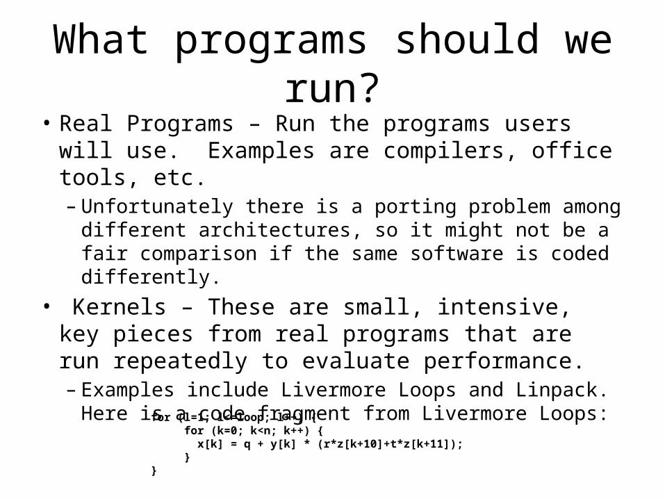
What programs should we run?• Real Programs – Run the programs users will use.
Examples are compilers, office tools, etc. – Unfortunately there is a porting problem among
different architectures, so it might not be a fair comparison if the same software is coded differently.
• Kernels – These are small, intensive, key pieces from real programs that are run repeatedly to evaluate performance.– Examples include Livermore Loops and Linpack. Here
is a code fragment from Livermore Loops:for (l=1; l<=loop; l++) {for (k=0; k<n; k++) { x[k] = q + y[k] * (r*z[k+10]+t*z[k+11]);}
}
Benchmarks
• Toy benchmarks - this includes small problems like quicksort, sieve of eratosthenes, etc.– They are best saved for CS201 programming assignments!
• Synthetic benchmarks - These are similar to kernels, but try to match the average frequency of operations and operands of a large set or programs.– Examples: Whetstone and Dhrystone– The problem is no user really runs these either. Programs
typically reside entirely in cache and don’t test the entire system performance!

Benchmarks
• Benchmark Suites - These are a collection of benchmarks together in an attempt to measure the performance of processors with a variety of applications.– Suffers from problems of OS support, compiler quality,
system components, etc.– Suites such as CrystalMark or the SPEC (www.spec.org)
benchmark seem to be required for the industry today, even if the results may be somewhat meaningless.
– http://www.spec.org/cpu2006/results/cpu2006.html

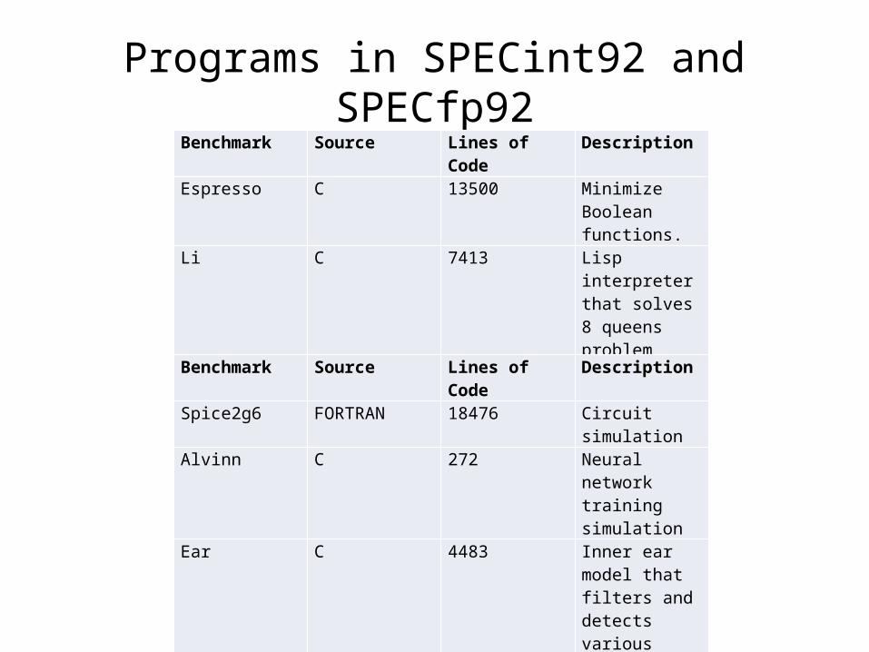
Programs in SPECint92 and SPECfp92
Benchmark Source Lines of Code DescriptionEspresso C 13500 Minimize
Boolean functions.
Li C 7413 Lisp interpreter that solves 8 queens problem
Compress C 1503 LZ compression on a 1Mb file
Gcc C 83589 GNU C Compiler
Benchmark Source Lines of Code DescriptionSpice2g6 FORTRAN 18476 Circuit simulationAlvinn C 272 Neural network
training simulation
Ear C 4483 Inner ear model that filters and detects various sounds
Su2cor FORTRAN 2514 Compute masses of elementary particles from Quark-Gluon theory
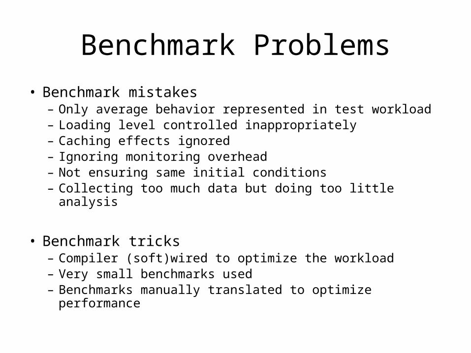
Benchmark Problems
• Benchmark mistakes– Only average behavior represented in test workload– Loading level controlled inappropriately– Caching effects ignored– Ignoring monitoring overhead– Not ensuring same initial conditions– Collecting too much data but doing too little analysis
• Benchmark tricks– Compiler (soft)wired to optimize the workload– Very small benchmarks used– Benchmarks manually translated to optimize performance

Benchmark Trick Example
• Certain flags during compilation can have a huge effect on final execution time for some tests– The Whetstone loop contains the following expression:
• SQRT(EXP(X))
– A brief analysis yields:
• It would be surprising to see such an optimization automatically performed by a compiler due to the expected rarity of encountering SQRT(EXP(X)). Nevertheless, several compilers did perform this optimization!
)2/(2/ XEXPee xx
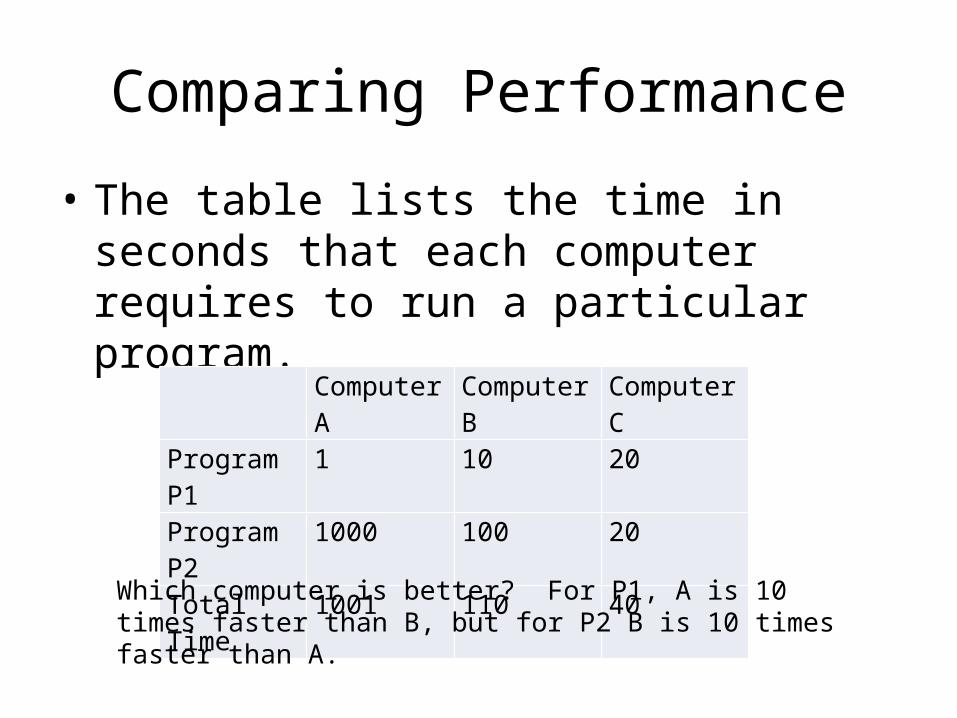
Comparing Performance
• The table lists the time in seconds that each computer requires to run a particular program.
Computer A Computer B Computer CProgram P1 1 10 20Program P2 1000 100 20Total Time 1001 110 40
Which computer is better? For P1, A is 10 times faster than B, but for P2 B is 10 times faster than A.

Total Execution TimeA consistent summary measure
• Simplest approach: compare relative performance in total execution time
• So then B is 9.1 times faster than A (1001/110), while C is 2.75 times faster than B. Of course this is all relative to the programs that are selected.

Other Total Execution Time Metrics
• Arithmetic mean
• Weighted arithmetic mean
• Normalize the execution time with respect to some reference machine. – Geometric mean
n
iiTime
n 1
1
n
iii TimeWeight
1
nn
i iimeRatioExecutionT1
1
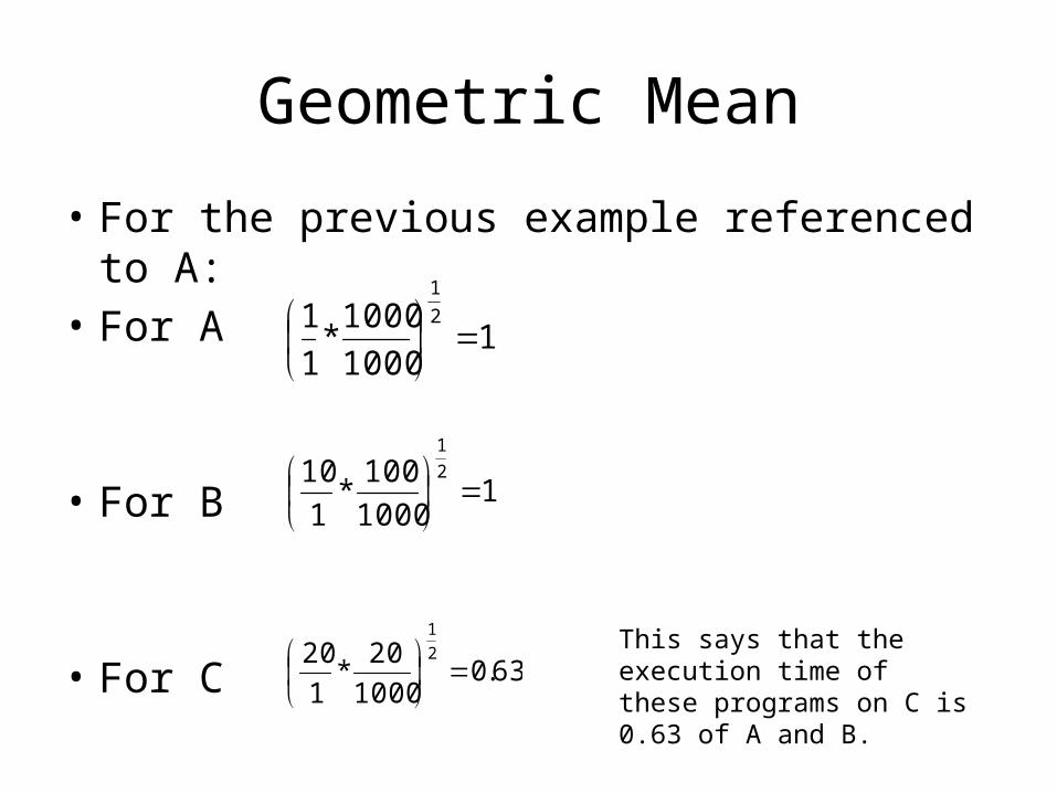
Geometric Mean
• For the previous example referenced to A:• For A
• For B
• For C
11000
1000*
1
1 2
1
11000
100*
1
10 2
1
63.01000
20*
1
20 2
1
This says that the execution
time of these programs on C is 0.63 of A and B.
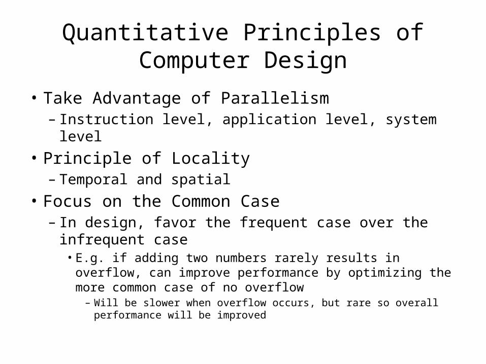
Quantitative Principles of Computer Design
• Take Advantage of Parallelism– Instruction level, application level, system level
• Principle of Locality– Temporal and spatial
• Focus on the Common Case– In design, favor the frequent case over the infrequent case
• E.g. if adding two numbers rarely results in overflow, can improve performance by optimizing the more common case of no overflow
– Will be slower when overflow occurs, but rare so overall performance will be improved

Amdahl’s Law
• The performance improvement to be gained from using some faster mode of execution is limited by the fraction of time the faster mode can be used.
• Speedup = (Performance for entire task using enhancement) / (Performance for entire task without enhancement)
• Another variant is based on the ratio of Execution times, where Execution time = 1/speedup.
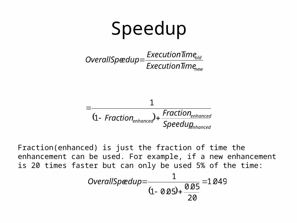
Speedup
enhanced
enhancedenhanced
new
old
Speedup
FractionFraction
imeExecutionT
imeExecutionTedupOverallSpe
1
1
Fraction(enhanced) is just the fraction of time the enhancement can be used. For example, if a new enhancement is 20 times faster but can only be used 5% of the time:
049.1
2005.0
05.01
1
edupOverallSpe
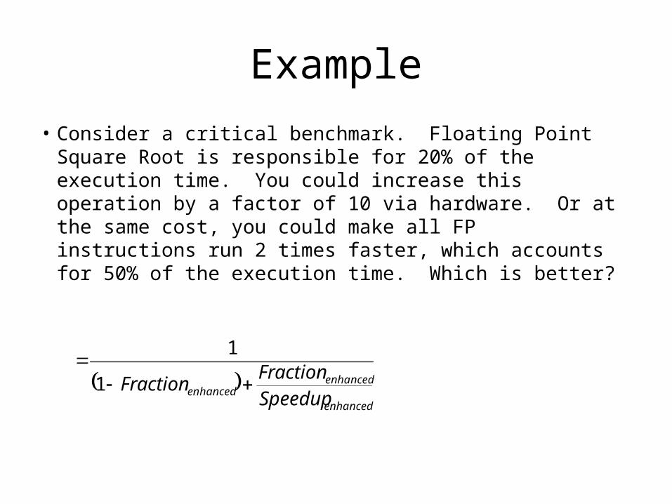
Example
• Consider a critical benchmark. Floating Point Square Root is responsible for 20% of the execution time. You could increase this operation by a factor of 10 via hardware. Or at the same cost, you could make all FP instructions run 2 times faster, which accounts for 50% of the execution time. Which is better?
enhanced
enhancedenhanced Speedup
FractionFraction
1
1
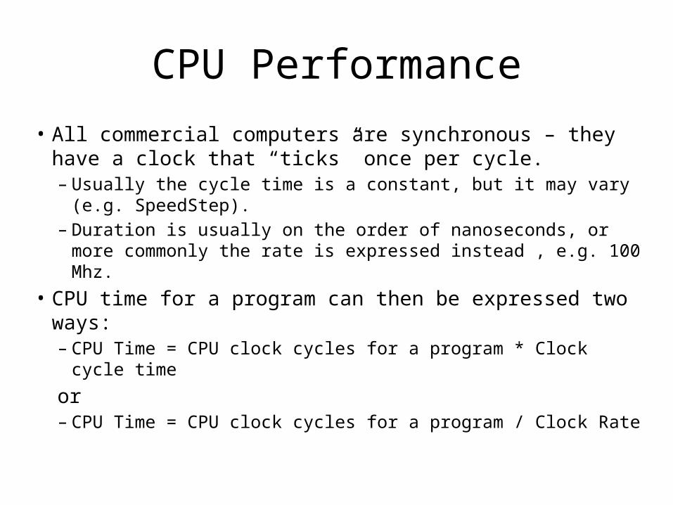
CPU Performance
• All commercial computers are synchronous – they have a clock that “ticks” once per cycle.– Usually the cycle time is a constant, but it may vary (e.g.
SpeedStep).– Duration is usually on the order of nanoseconds, or more
commonly the rate is expressed instead , e.g. 100 Mhz. • CPU time for a program can then be expressed two ways:
– CPU Time = CPU clock cycles for a program * Clock cycle time
or– CPU Time = CPU clock cycles for a program / Clock Rate

Cycles Per Instruction• We can count the number of instructions executed – the
instruction path length or Instruction Count (IC). Given IC and the number of clock cycles we can calculate the average number of clock cycles per instruction, or CPI:– CPI (Ave # clock cycles per instr) = CPU clock cycles for a program / IC
• With a little algebraic manipulation we can use CPI to compute CPU Time:– CPU clock cycles for a program = CPI * IC
Substitute this in for CPU Time..
– CPU Time = CPI * IC * Clock Cycle Time
Or
– CPU Time = CPI * IC / ClockRate
CPI
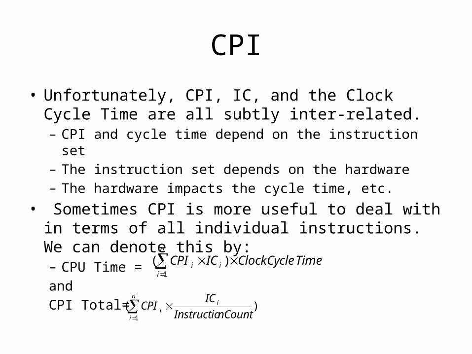
• Unfortunately, CPI, IC, and the Clock Cycle Time are all subtly inter-related. – CPI and cycle time depend on the instruction set– The instruction set depends on the hardware– The hardware impacts the cycle time, etc.
• Sometimes CPI is more useful to deal with in terms of all individual instructions. We can denote this by:– CPU Time = andCPI Total=
TimeClockCycleICCPIn
iii
)(1
)(1 nCountInstructio
ICCPI i
n
ii
CPI Example
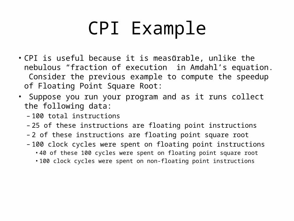
• CPI is useful because it is measurable, unlike the nebulous “fraction of execution” in Amdahl’s equation. Consider the previous example to compute the speedup of Floating Point Square Root:
• Suppose you run your program and as it runs collect the following data:– 100 total instructions– 25 of these instructions are floating point instructions– 2 of these instructions are floating point square root– 100 clock cycles were spent on floating point instructions
• 40 of these 100 cycles were spent on floating point square root• 100 clock cycles were spent on non-floating point instructions

CPI Example
• Frequency of FP operations = 25/100 = 0.25• Frequency of FPSQ operations = 2/100 = 0.02• Ave CPI of FP operations = 100 / 25 = 4• Ave CPI of FPSQ operations = 40 / 2 = 20• Ave CPI of non-FP operations = 100 / 75 = 1.33 • If we could reduce the CPI of FPSQ by 10 (down to 2),
or reduce the CPI of all FP operations by 2, which is better?– Will calculate in class

Measuring Components of CPU Performance
• Cycle Time is easy to measure for an existing CPU (whatever frequency it is running at).
• Cycle Time is hard to measure for a CPU in design! The logic design, VLSI process, simulations, and timing analysis need to be done.
• IC – This is one thing that is relatively easy to measure, just count up the instructions. This can be done with instruction trace, logging, or simulation tools.
• CPI – This can be difficult to measure exactly because it depends on the processor organization as well as the instruction stream. Pipelining and caching will affect the CPI, but it is possible to simulate the system in design and estimate the CPI.
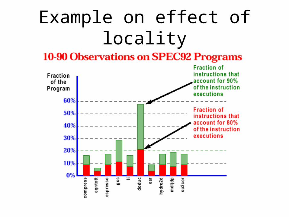
Example on effect of locality

Common Fallacies, Pitfalls
• Falling prey to Amdahl’s Law– Should measure speedup before spending effort
to enhance it• Single point of failure
– E.g. single fan may limit reliability of the disk subsystem
• Fallacy: The cost of the processor dominates the cost of the system

Common Fallacies, Pitfalls
• Fallacy: Benchmarks remain valid indefinitely– Benchmark reverse engineering in compilers
• Fallacy: The rated mean time to failure of X is 1,200,000 hours or almost 140 years, so X will practically never fail– More useful measure would be % of disks that fail
• Fallacy: Peak performance tracks observed performance– Example: Alpha in 1994 announced as being capable of
executing 1.2 billion instructions per second at its 300 Mhz clock rate.

Common Fallacies, Pitfalls
• Fault detection can lower availability– Hardware has a lot of state that is not always
critical to proper operation• E.g. if cache prefetch fails, program will still work, but a
fault detection mechanism could crash the program or raise errors that take time to process
• Less than 30% of operations on the critical path for Itanium 2
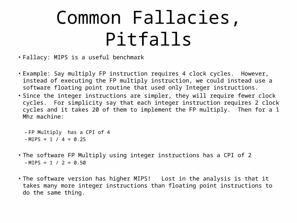
Common Fallacies, Pitfalls• Fallacy: MIPS is a useful benchmark
• Example: Say multiply FP instruction requires 4 clock cycles. However, instead of executing the FP multiply instruction, we could instead use a software floating point routine that used only Integer instructions.
• Since the integer instructions are simpler, they will require fewer clock cycles. For simplicity say that each integer instruction requires 2 clock cycles and it takes 20 of them to implement the FP multiply. Then for a 1 Mhz machine:
– FP Multiply has a CPI of 4 – MIPS = 1 / 4 = 0.25
• The software FP Multiply using integer instructions has a CPI of 2– MIPS = 1 / 2 = 0.50
• The software version has higher MIPS! Lost in the analysis is that it takes many more integer instructions than floating point instructions to do the same thing.