Connecting Markets East & West

© Nomura February 2018

Fundamental Review of The Trading Book – The road to IMA

ICMA SMPC 6 February 2018 Eduardo Epperlein, Global Head of Risk Methodology

The views and opinions expressed herein are those of the author and do not necessarily reflect the views of Nomura Holdings, its

affiliates, or its employees.

Agenda

NMRF PL attribution

1

Non-Modellable Risk Factors (NMRF)

2

NMRF is a capital add-on based on non the modellability of risk factors

NMRF was designed to formalize the existing “Risks not in VaR” (RniV) framework originally developed by the UK PRA

For Nomura, about 65 % of the risk factor population can be classified as non-modellable, with an average liquidity horizon (LH)

of ~130/140 days. Below is a breakdown per main risk classes.

Nomura supports the industry pooling of data, but the data outcome is still uncertain

Spot risk factors

Risk class

% NMRF Mean NMRF LH (in days)

Std Dev NMRF LH (in days)

IMA LH range

Equity 61% 82 53 10-20

Rates 38% 139 90 10-20

FX 7% 113 110 10-20

Credit 67% 149 85 20-60

Volatility risk factors

Risk class % NMRF Mean NMRF LH (in days)

Std Dev NMRF LH (in days)

IMA LH range

Equity ATM Vol 95% 142 69 20-60

Rates ATM Vol 78% 147 79 60

FX ATM Vol 82% 129 74 40

3

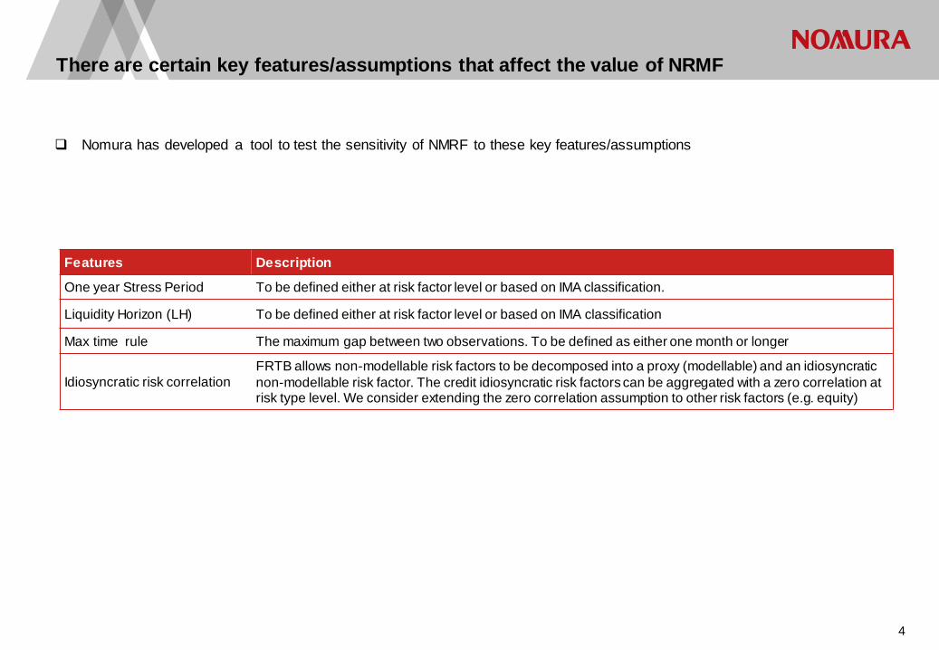
There are certain key features/assumptions that affect the value of NRMF

Nomura has developed a tool to test the sensitivity of NMRF to these key features/assumptions

Features Description

One year Stress Period To be defined either at risk factor level or based on IMA classification.

Liquidity Horizon (LH) To be defined either at risk factor level or based on IMA classification

Max time rule The maximum gap between two observations. To be defined as either one month or longer

Idiosyncratic risk correlation

FRTB allows non-modellable risk factors to be decomposed into a proxy (modellable) and an idiosyncratic

non-modellable risk factor. The credit idiosyncratic risk factors can be aggregated with a zero correlation at risk type level. We consider extending the zero correlation assumption to other risk factors (e.g. equity)

4

Nomura analysed two NMRF capital scenarios

In Basel 2.5, RniV capital is much smaller than NMRF capital. RniV ~ 0.15 x IMA ESF.

For the FRTB QIS Nomura submitted the more realistic scenario. Even so, the resultant NMRF capital ~ IMA ESF capital.

Do we really think that we have a 100% uncertainty in the VaR engine, let alone 1000%?

5

By varying the assumptions we observe enormous variability in

the capital impact

* All Equity, FX, G10 Rates are assumed modellable, the NMRF liquidity horizon is assumed to be aligned to IMA liquidity horizon, the 1 month modellability criteria was relaxed

Assumptions Strict rule

interpretation More Realistic

Liquidity Horizon Risk factor

specific IMA based

Stress Period Risk factor

specific IMA based

Zero Correlation

Aggregation Credit Credit

Transaction Data Internal only Internal + partially

external*

Observability

Rule

Min 24 per year

and max 1M gap Min 24 per year only

NMRF: Assumption sensitivity analysis

6

A breakdown of these two scenario provide some information on most sensitive parameters.

Scenario Realistic Scenario 1 Scenario 2 Scenario 3 NMRF Strict

Definitions

Observability Test # Trades Count Only # Trades Count Only # Trades Count Only # Trades Count Only # Trades Count + 1M Max Gap

Liquidity Horizon IMA LH IMA LH IMA LH NMRF LH NMRF LH

Stress Period

Fixed Fixed Rolling Rolling Rolling

Zero correlation for

specific risk credit spread credit spread credit spread credit spread credit spread

Modellable RF Data

Equity/FX/G10 Rate Spot

modellable + Nomura

trades

Nomura trades Nomura trades Nomura trades Nomura trades

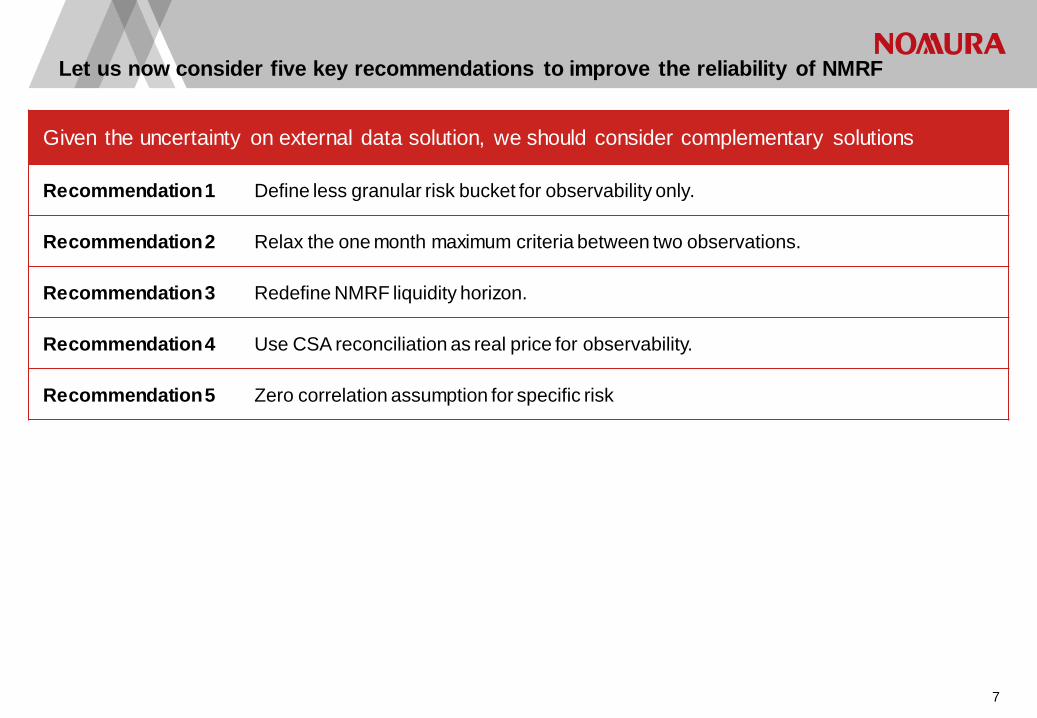
Let us now consider five key recommendations to improve the reliability of NMRF

Given the uncertainty on external data solution, we should consider complementary solutions

Recommendation 1 Define less granular risk bucket for observability only.

Recommendation 2 Relax the one month maximum criteria between two observations.

Recommendation 3 Redefine NMRF liquidity horizon.

Recommendation 4 Use CSA reconciliation as real price for observability.

Recommendation 5 Zero correlation assumption for specific risk

7

NMRF Recommendation 1: Define less granular risk buckets for observability only

PLA

Test is designed to ensure appropriate risk

factor coverage.

Defining not enough risk factors can lead

to PLA failures and hence IMA ineligibility

Higher granularity – prerequisite

for internal model usage

Lower granularity –

prerequisite for reasonable

NMRF

NMRF

Only modellable risk factors can be

capitalized in IMA ESF model

All others are capitalized via NMRF

Defining too many risk factors can lead to

unreasonable NMRF

Industry recognize that risk factor granularity has contradictive requirement between NMRF and P&L attribution (PLA).

Risk factor definition/cannot be generally aligned across firms/vendors, with consequent bucketing.

Recommendation 1: Introduce risk factor buckets for the observability assessment only. A reasonable starting point could be the SBA risk factors.

8

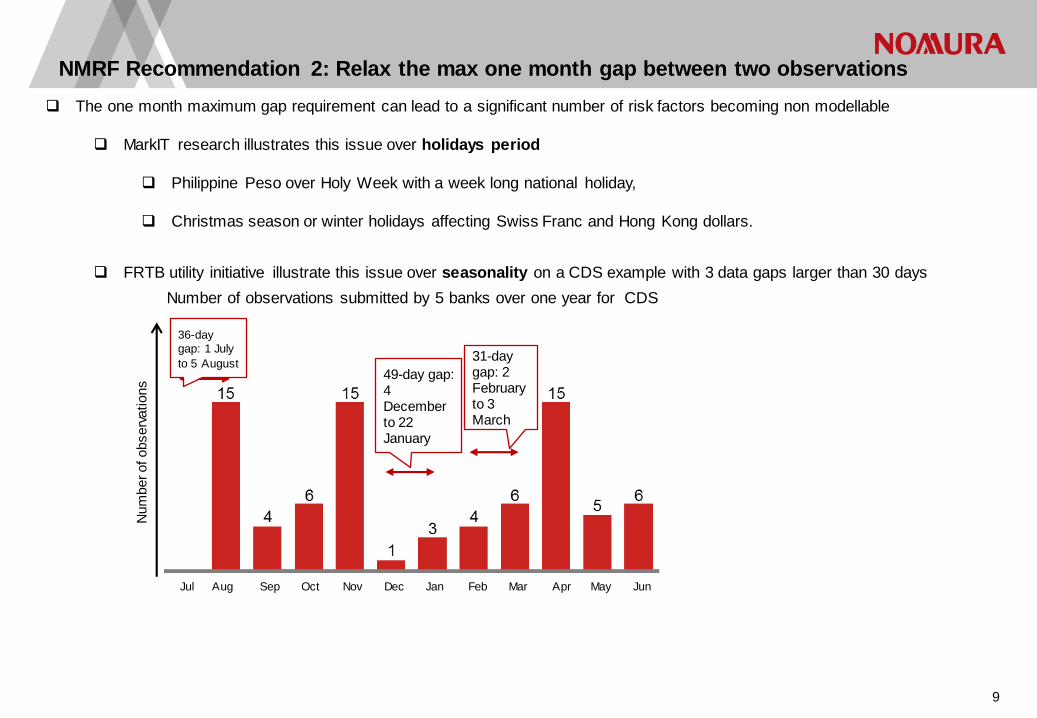
NMRF Recommendation 2: Relax the max one month gap between two observations

The one month maximum gap requirement can lead to a significant number of risk factors becoming non modellable

MarkIT research illustrates this issue over holidays period

Philippine Peso over Holy Week with a week long national holiday,

Christmas season or winter holidays affecting Swiss Franc and Hong Kong dollars.

FRTB utility initiative illustrate this issue over seasonality on a CDS example with 3 data gaps larger than 30 days

36-day

gap: 1 July

to 5 August 49-day gap: 4 December to 22 January

31-day gap: 2 February to 3 March

Number of observations submitted by 5 banks over one year for CDS

Jul Aug Sep Oct Nov Dec Jan Feb Mar Apr May Jun

Num

ber of observ

ations

9

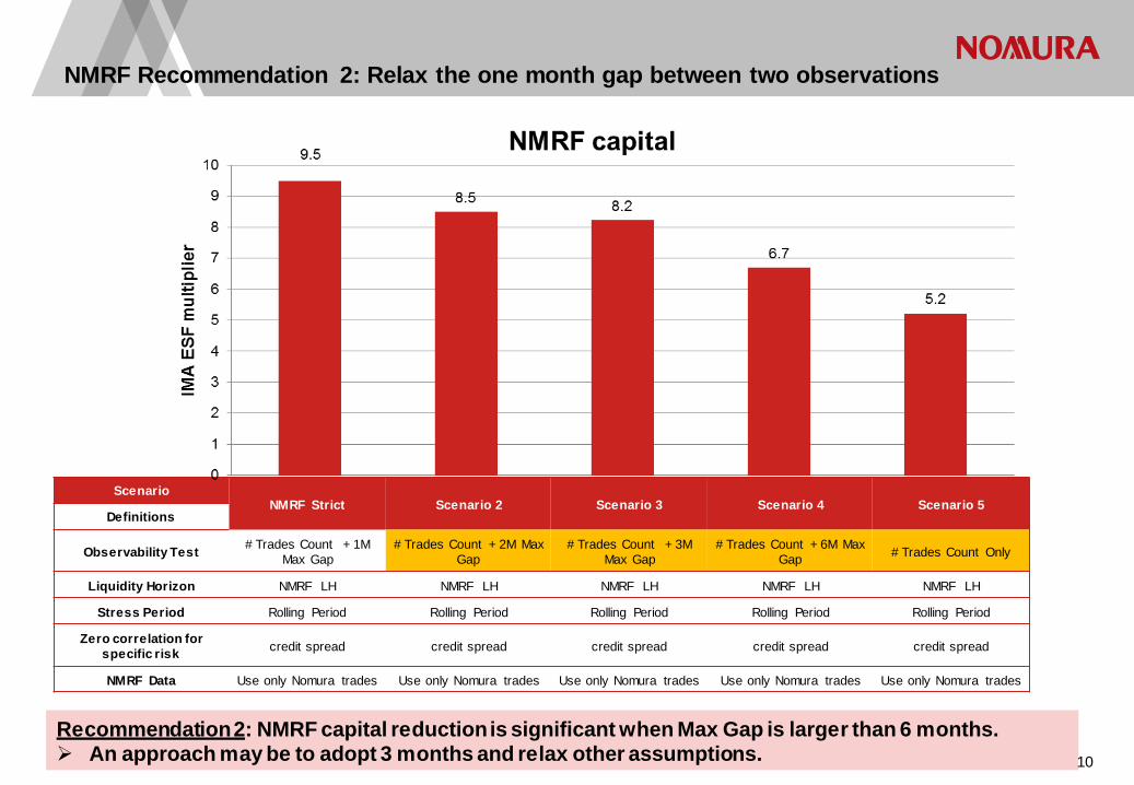
NMRF Recommendation 2: Relax the one month gap between two observations

Recommendation 2: NMRF capital reduction is significant when Max Gap is larger than 6 months. An approach may be to adopt 3 months and relax other assumptions.

Scenario NMRF Strict Scenario 2 Scenario 3 Scenario 4 Scenario 5

Definitions

Observability Test # Trades Count + 1M

Max Gap

# Trades Count + 2M Max

Gap

# Trades Count + 3M

Max Gap

# Trades Count + 6M Max

Gap # Trades Count Only

Liquidity Horizon NMRF LH NMRF LH NMRF LH NMRF LH NMRF LH

Stress Period Rolling Period Rolling Period Rolling Period Rolling Period Rolling Period

Zero correlation for

specific risk credit spread credit spread credit spread credit spread credit spread

NMRF Data Use only Nomura trades Use only Nomura trades Use only Nomura trades Use only Nomura trades Use only Nomura trades

10

NMRF Recommendation 3: Redefine NMRF liquidity horizon

The NMRF liquidity horizon can be extremely punitive for certain risk factors with horizon going up to 1year.

The below graph corresponds to two NMRF liquidity horizon distributions for credit spot and equity volatility. The grey column corresponds

to the IMA ESF liquidity horizon level.

Observations/conclusions

In 60-70% of cases, NMRF liquidity horizons are higher than IMA liquidity horizon.

In 40% of cases, NMRF liquidity horizons are more than twice IMA liquidity horizon.

Recommendation 3: Redefine NMRF liquidity horizon. A reasonable starting point would be to align liquidity horizon to IMA ESF. 11

Background

• Reconciliation of collateral levels for bi-laterally cleared derivatives is an established operational process

• Such process is required by existing regulation covering the mitigation of operational and counterparty credit risk (for example, Article

11 of EMIR)

• Results in tangible economic consequences – i.e. the exchange of collateral

• Data at the trade level is readily available from existing vendor products. Contract details are well-defined to facilitate the mapping to

risk factors

• When reconciliation is achieved, it effectively means that 2 parties with opposite economic interests are aligned on price

NMRF Recommendation 4: Use of CSA reconciliation for real-price source

Recommendation

The recommendation is that – subject to certain standards – the prices used in CSA reconciliation should be permissible as a source of

real-price observations in the risk factor modellability test. Those standards are:

• Visibility of prices at the trade level

• Agreement between counterparties on the terms of each trade

• Independent submission of trade-level prices by each counterparty

• Agreement on price between counterparties to within specified thresholds.

12

NMRF Recommendation 5: Zero correlation on residual risk

Assuming all NMRF equity are decomposed as proxy + residual, the graph below shows the NMRF capital impact of aggregating

equity residual risk with zero correlation.

Scenario NMRF Strict Scenario 1

Definitions

Observability Test # Trades Count + 1M Max Gap # Trades Count + 1M Max Gap

Liquidity Horizon NMRF LH

NMRF LH

Stress Period Rolling Period

Rolling Period

Zero correlation for specific

risk credit spread credit spread + equity spot/vol

NMRF Data Use only Nomura trades Use only Nomura trades

Recommendation 5: Review NMRF aggregation. Consider zero correlation for residual risk aggregation.

13

PL attribution (PLA)

14

Background

15

P&L Attribution (PLA) is a new concept for Internal Model Approach (IMA) approval, introduced under FRTB

• We must compare two quantities:

Hypothetical P&L (HPL): The P&L produced by revaluing the positions held at the end of the previous day using the market data at the end of the current day – a familiar concept from backtesting

Risk Theoretical P&L (RTPL): the ex-ante P&L ‘from the risk model’ – a new concept

To compute the Unexplained P&L (UPL), defined as the difference of the two.

• Given these two quantities, we measure two statistics:

• The Mean Ratio (MR) and Variance Ratio (VR) are computed every month, and reported to the regulator

If a desk violates the threshold on either metric more than 3 months out of 12, model approval is lost.

PLA is the number one industry concern on the final FRTB rule

• This is driven by the high number of desks failing in test exercises, and the associated capital penalty

What are the key issues, and how might they be fixed?

𝑀𝑅 =|𝑀𝑒𝑎𝑛 𝑈𝑃𝐿 |

𝑆𝑡𝑑𝐷𝑒𝑣 𝐻𝑃𝐿< 10% 𝑉𝑅 =

𝑉𝑎𝑟 𝑈𝑃𝐿

𝑉𝑎𝑟 𝐻𝑃𝐿< 20%

P&L Attribution

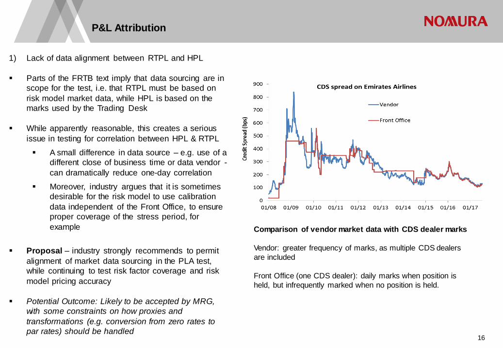
1) Lack of data alignment between RTPL and HPL

Parts of the FRTB text imply that data sourcing are in

scope for the test, i.e. that RTPL must be based on

risk model market data, while HPL is based on the

marks used by the Trading Desk

While apparently reasonable, this creates a serious

issue in testing for correlation between HPL & RTPL

A small difference in data source – e.g. use of a

different close of business time or data vendor -

can dramatically reduce one-day correlation

Moreover, industry argues that it is sometimes

desirable for the risk model to use calibration

data independent of the Front Office, to ensure

proper coverage of the stress period, for

example

Proposal – industry strongly recommends to permit

alignment of market data sourcing in the PLA test,

while continuing to test risk factor coverage and risk

model pricing accuracy

Potential Outcome: Likely to be accepted by MRG,

with some constraints on how proxies and

transformations (e.g. conversion from zero rates to

par rates) should be handled

Comparison of vendor market data with CDS dealer marks

Vendor: greater frequency of marks, as multiple CDS dealers

are included

Front Office (one CDS dealer): daily marks when position is

held, but infrequently marked when no position is held.

16

P&L Attribution

2) Penalty function for failing P&L Attribution

A desk which fails the PLA test – defined as either ratio falling above the threshold for more than 3 months out of 12

– immediately moves on to the standardised approach, with potentially huge jump in capital:

Considering the novel form and hence unpredictable of PLA, imposing such a severe penalty seems risky .

Having such a binary outcome can lead to instability in regulatory capital, complicating capital planning for

firms, and for supervisors via ICAAP, CCAR, etc

Proposal: industry recommends to have a smooth capital penalty as the PLA pass rates deteriorates, for example

by making a linear interpolation of SBA and IMA for the bank as a whole.

And to allow a temporary ‘Amber zone’ for failing desks, where the issues can be diagnosed, before capital

penalty is applied

Potential Outcome: MRG seems inclined to use a traffic light test, introducing an Amber Zone for moderately poor

PLA performance. Desks in this zone would see a capital add-on, but less punitive than full SBA

Source: ISDA/GFMA/IIF FRTB QIS analysis, July 2017

17

P&L Attribution

3) The metric used to test PLA – especially the variance ratio – can be unstable

The use of Var[HPL] in the denominator of the Variance Ratio can lead to a very high ratio where HPL is small in absolute

terms, such as for a well hedged Trading Desk.

Also, it can be shown that the VR moderately favours desks where Var [RTPL] < Var [HPL], i.e. where the Risk model

underestimates the true volatility of P&L

A further issue is that the use of monthly data (i.e. ~22 one day samples) can lead to sampling error in the results

𝑀𝑒𝑎𝑛 𝑅𝑎𝑡𝑖𝑜 (𝑀𝑅) =|𝑀𝑒𝑎𝑛 𝑈𝑃𝐿 |

𝑆𝑡𝑑𝐷𝑒𝑣 𝐻𝑃𝐿< 10% 𝑉𝑎𝑟𝑖𝑎𝑛𝑐𝑒 𝑅𝑎𝑡𝑖𝑜(𝑉𝑅) =

𝑉𝑎𝑟 𝑈𝑃𝐿

𝑉𝑎𝑟 𝐻𝑃𝐿< 20%

Proposal: maintain the spirit of the test by measuring the similarity

and correlation of RTPL and HPL, but using better understood

statistical metrics.

For example, the Kolmogorov-Smirnov test to compare the

shape of the distributions, and a non-parametric measure like

Spearman’s rho to measure correlation

Use rolling annual data in the test, to minimise sample noise

Potential Outcome: likely to been accepted by MRG, except that

Chi-squared test may be used rather than Kolmogorov-Smirnov

Illustration of KS test, which measures the

size of the highlighted area 18

P&L Attribution

4) Calibration of the test is very difficulty, until firms can provide reliable input data

Regardless of the specific statistics chosen, the regulators need to calibrate the thresholds for failing the test

The obvious solution is to gather data via the QIS process, but this is difficult for firms to provide,

In particular, the system and process changes to develop RTPL are very significant, and firms have been

reluctant to invest in this while the PLA rules remain uncertain

Proposal: the industry has tried to tackle this issue via the construction of hypothetical datasets, with stylized

representations of what real HPL and RTPL may look like. But it is very difficult to be sure that any hypothetical data

are truly representative

Instead the industry proposes to have a temporary calibration period post FRTB go-live, where firms must

submit RTPL and HPL data and explain results to regulators, but without a binding test.

Likely Outcome: a non-binding calibration phase is not likely to be accepted. Instead the FRTB go-live is being

pushed back by national regulators – see for example recent draft European Council report proposing a three or

four year delay following the entry into force of the FRTB regulations

Jan 2019 Jan 2020 Jan 2021 Jan 2022 Jan 2023 Jan 2024 Jan 2018

Basel rule

finalization

CRR II “entry into

force”? EU go-live? Full capital

impact?

Model review and

approval

Phased capital

impact

Potential EU FRTB timeline

19