Embed Size (px)
Citation preview

Rep. Prog. Phys.63 (2000) 455–503. Printed in the UK PII: S0034-4885(00)72320-7
Fundamental quantum optics in structured reservoirs
P Lambropoulos†‡, Georgios M Nikolopoulos†‡, Torben R Nielsen†§ and Søren Bay†† Max-Planck-Institut fur Quantenoptik, Hans-Kopfermann-Str. 1, 85748 Garching, Germany‡ Institute of Electronic Structure and Laser, Forth, PO Box 1527, Heraklion 71110, Crete, Greece and Departmentof Physics, University of Crete, Crete, Greece§ Niels Bohr Institute, Ørsted Laboratory, Universitetsparken 5, DK-2100 Copenhagen Ø, Denmark
Received 16 July 1999, in final form 16 November 1999
Abstract
We review basic quantum electrodynamics and quantum optics aspects in microstructures thatexhibit a gap in the spectrum of the electromagnetic radiation they support, known as photoniccrystals. After a brief sketch of the properties of such materials we discuss the behaviour offew-level atoms or collections thereof with transition frequencies inside and in the vicinity ofthe gap. The discussion is cast in terms of a unified formalism which facilitates the comparisonwith standard cavity–atom physics.
0034-4885/00/040455+49$90.00 © 2000 IOP Publishing Ltd 455

456 P Lambropoulos et al
Contents
Page1. Introduction 4572. Photonic crystals 4603. The two-level atom (TLA) in a structured reservoir 461
3.1. Formalism 4613.2. TLA in open space 4643.3. TLA in a cavity 4653.4. The TLA in a PBG medium 4683.5. Comparative discussion 473
4. Beyond the TLA 4784.1. Spontaneous decay in three-level systems 4784.2. Externally driven three-level systems 484
5. Atom–atom interaction 4866. Superradiance 4927. Beyond one photon in the reservoir 4978. Summary and outlook 499
References 500

Fundamental quantum optics in structured reservoirs 457
1. Introduction
The behaviour of small systems (few degrees of freedom) coupled to dissipative reservoirsrepresents a central theme of quantum optics. Typical systems of particular interest in quantumoptics are few-level atoms (or collections thereof) coupled to the radiation field which, in oneform or another, involves a dissipative reservoir. The problems and phenomena arising in thatcontext do in fact belong to the more general class of dissipative quantum systems (Weiss1993).
In its simplest form, which is useful to recall here, the problem consists of an atomin its first excited state from which it is returned to its ground state through an allowedelectric dipole transition, assuming the atom to be situated in open space so that the emittedradiation propagates away never returning to the position of the atom. This is a prototype ofirreversible decay of a prepared state, as well as a classic manifestation of the quantizationof the electromagnetic field. Together with the vacuum shift, with which the width of thedecaying state is intimately connected through a dispersion relation, it features in all texts ofquantum electrodynamics (QED) (Sakurai 1995).
With the advent of the laser, high-resolution spectroscopy and single-atom physics,that standard QED problem acquired further dimensions, beyond the width and shift of thedecaying state. The statistical properties of the emitted radiation as reflected in its correlationfunctions, the difference between single- and many-atom fluorescence and the phenomenonof superradiance (SR), whose origins actually predate the laser, are examples of the broaderscope in which spontaneous radiative decay is now viewed.
Technological developments, in the form of high quality and finesse cavities, led to theextension of such studies into yet another direction, which has come to be known as cavityQED (Haroche 1984, Dobiasch and Walther 1985, Walther 1992, Meystre 1992, Hansch andWalther 1999). The point of departure is the realization that spontaneous decay and vacuumshift are not independent of the geometry and associated mode structure of the electromagneticfield in which the atom is embedded (Kleppner 1981). Take for example an atom, excited tosome Rydberg state, placed inside a microwave cavity of high quality factorQ (say 109–1010)and mode spacing larger than the mode width. If the frequency of the transition from the initialRydberg state to the nearest one (with which a nonzero electric dipole matrix element exists)matches one of the low modes of the cavity, spontaneous emission is enhanced; whereas it isseverely inhibited if the atomic transition is detuned from all cavity modes by an amount largecompared with the width of the mode. In the case of exact resonance between atomic transitionand cavity mode, the spontaneously emitted photon can be reabsorbed by the atom, leadingthus to oscillations beginning with the radiation field in the vacuum state. This phenomenon,known as vacuum Rabi oscillations, represents a sharp contrast between the decay of anexcited state in open space and its temporal evolution inside a confined volume, with moreor less reflecting walls, so that radiation deposited by the atom inside the cavity takes a longtime to be dissipated into the environment through losses at the walls. This has made possiblethe micromaser, pumped by the transit of excited Rydberg atoms through a microwave cavity.It has been studied in great detail and in a variety of conditions, from the single atom at atime inside the cavity to the case of SR (Haroche 1992, Raithelet al 1994). The phenomenoncontinues to attract attention, most recently even in the context of creating entangled quantumstates as prototypes of quantum communication schemes (Maitreet al 1997, Steane 1998).
Thus, unlike spontaneous decay in open space, the decay of the excited state is enhancedand reversible if the atomic transition is on resonance with the cavity mode, while it is delayedfor an atomic frequency sufficiently detuned from the cavity mode. Qualitatively speaking,the atom can deposit its energy in the form of radiation only if the geometry and conditions of

458 P Lambropoulos et al
surrounding space allow it. A nice recent pedagogical treatment of that phenomenon has beenpresented by Giessenet al (1996). Also, the vacuum shift depends on and can be modifiedby the manipulation of mode structure of the surrounding space. Placing, for example, aRydberg atom between two parallel metallic plates, whose distance is of the order of thewavelength of the radiation connecting the initial state to the energetically adjacent ones,causes a modification of the vacuum shift as virtual transitions to such states are eliminated,simply because the longest wavelength allowed vertically between the plates is equal to twicetheir distance (Dobiaschet al 1985, Hindset al 1991, Marroccoet al 1998).
Technological limitations have until recently allowed cavities of very highQ factor onlyin the microwave range of wavelengths. That is why most of the relevant studies havebeen concerned with atoms in Rydberg states. Rapid progress in high-quality microcavities,however, is making possible the contemplation of analogous studies in the optical range.Discussions about the implementation of a microlaser have already appeared in the literature(An et al 1994, Yamamoto and Slusher 1993).
Cavity modes have peaked, but smooth, lineshapes, with the Lorentzian being a reasonablygood model. Even in a very high-quality cavity, with a very narrow lineshape, a photondeposited in the cavity may be retained for a very long time, but it will eventually belost in the environment. Consequently, an excited atom with transition frequency detunedfrom the nearest cavity mode by many mode widths may take a long time to decay but iteventually will, dissipating its energy of excitation into the environment. This means that themathematical model representing this situation predicts that, as the time tends to infinity, theatomic population tends to the lower state and the cavity to a state of no excitation, other than thatdictated by the temperature of its environment. Throughout this review, we will be assumingT = 0 K. Basically, this can be related to the fact that a Lorentzian (or even a Gaussian forthat matter), no matter how narrow, has wings extending to infinity, as a consequence of whichan atom is not protected from decay, no matter how far from the cavity mode its transitionfrequency may be.
A drastically different situation arose when it was realized that it was possible to createenvironments in which the spectrum of the electromagnetic field exhibits gaps in frequency.In other words, no radiation over some extended range of frequency can propagate in thatenvironment. Simply stated, with a quantitative description to follow later on, an excited atomwhose transition frequency falls in the range of that gap should at first sight never decay, evenin the limit of the time tending to infinity. These are referred to as photonic band gap (PBG)materials or PBG crystals or even photonic crystals (Joannopoulos 1995). The original ideaof light localization is due to John (1987) and independently Yablonovitch (1987), who wasalso the first to construct such a material exhibiting a gap in the microwave range. Followingthe initial suggestions, theoretical as well as experimental work has mushroomed in the questof improving their properties, while at the same time pushing the range of the gap towardsshorter wavelengths.
Not surprisingly, these developments immediately led to the investigation of questionsrepresenting the natural extension of the ideas of cavity QED to the environments promisedby these novel materials. Spearheaded by John and collaborators and then quickly spreadingto many groups throughout the world, we have witnessed an avalanche of papers dealing withthe questions normally debated in quantum optics, extrapolated now to PBG materials, or atleast their theoretical properties under somewhat idealized conditions. This line of activity isoften referred to as quantum optics in PBG materials, and is for the time being dominated bytheoretical elaborations.
The issues that have been addressed mirror those of cavity QED: i.e. the behaviour oftwo- or few-level atoms or collections thereof, assuming that they can be placed inside such

Fundamental quantum optics in structured reservoirs 459
materials. As already alluded to above, some features familiar from cavity QED are expectedto be different: as for example the complete absence of decay of a two level atom. Whetherthis represents a qualitative or quantitative departure from the behaviour in cavities will bediscussed as we go along. In pondering such, possibly semantic, questions it is relevant tokeep in mind that similar issues can arise and have in fact been discussed in the context ofstandard waveguides, where the density of states (DOS) of the radiation field bears considerableresemblance to that of PBG materials.
The DOS is the fundamental feature that determines the behaviour of the system ‘atom plusfield’ and characterizes the various types of environments. The form and analytical propertiesof the DOS dictate the type of the approximations that are permissible in formulating theequations governing the time development of the system. In that respect, a smooth DOS,without singularities, usually allows the so-called Born and often Markov approximation, tobe detailed later on, which make possible the derivation of a master equation. Such is the caseof the DOS inside a cavity. A Lorentzian, no matter how narrow, is a smooth function. At theother extreme, the DOS that, under some idealized circumstances, can be taken as a workingapproximation to a PBG environment is singular, which as we shall see precludes both theBorn and the Markov approximations, thus ruling out the rigorous use of a master equation.It has in the meantime turned out that non-Markovian aspects appear in other quite differentcontexts, such as the atom laser or ultrafast nonlinear processes in semiconductors. Thusquantum optics, which has throughout its development relied on the master equation, mustin this new context cope without a Markovian master equation of unquestioned and generalvalidity. And that is perhaps the central issue involved, one way or another, in all of the specificproblems that have been and are being explored under the banner of the quantum optics inPBG materials. It is true that the Monte Carlo wavefunction (MCWF) approach (Dalibardet al1992, Mølmeret al1993), representing now a standard tool in quantum optics, especiallywhen quantization of the centre-of-mass motion is involved as in laser cooling, was invented inorder to sidestep the master equation. The reasons, however, were not conceptual. The masterequation is still valid in that context, but too complicated to cope computationally: there beingtoo many equations to handle.
The situation in the PBG case is different at the fundamental level and reflects a difficultystemming from the many-body nature of the system that leads to that particular, or similar,DOS. Part of the issues to be dealt with, therefore, have to do with alternative approachessuch as the direct solution of the wave equation, whenever possible, or the constructionof alternative models sharing some of the properties (or rather the consequences) with theunconventional DOS. In some problems, one can formulate the equations of motion for theHeisenberg operators and proceed by adopting suitable decorrelation approximations in thehierarchy of differential equations governing the time evolution of the correlation functions.Physical arguments often provide strong and convincing justification for such approaches,but it is also useful to add insight through alternative, somewhat simplified, models lendingthemselves to a treatment without decorrelation, provided that the essential physics is nottossed out in the process.
The general ideas anticipating the basic QED effects in PBG media were outlined by John(1991) quite early and his work on the typical phenomena, such as the photon–atom boundstate, atom–atom resonance dipole–dipole interaction (RDDI) and SR up to about (1994) hasbeen reviewed in John (1994). Many of the basic issues, especially in connection with RDDIin PBG structures, were also anticipated and discussed fairly early by Kurizki (1990). Kofmanet al (1994) have presented a rather detailed elaboration on the features of atomic decay inmodel DOS representing PBG structures. Their paper was in fact part of a special issue oftheJournal of Modern Optics(1994) dedicated to PBG structures, with emphasis on quantum

460 P Lambropoulos et al
optics aspects. Thus, adhering to the spirit of this journal, our purpose in the following pagesis to present an overview of the basic quantum optics effects in the context of PBG structuresas they have developed through up to 1999. To streamline the exposition, we have chosena particular formalism in terms of the resolvent operator which allows the discussion of alleffects included herein from a unified standpoint. It does not differ in substance from theformulation used by others, being simply a matter of preference and economy in equations.Neither space nor the scope of this review allow the detailed mathematical elaboration of allissues. We hope to have included sufficient detail to give the flavour of the physics involved,as well as a guide to the existing literature. Although we have endeavored to cite most ofthe work published by the numerous groups involved in relevant research, given the rate ofappearance of papers, oversights are inevitable.
The paper is structured in the order of complexity of the effects discussed. Thus, aftera brief summary of basic facts about photonic crystals in section 2, the simplest system,namely the two-level atom, is analysed in section 3, which serves also as an introduction tothe formalism, followed by section 4 dealing with three-level models. Section 5 addressesthe RDDI between two atoms, while section 6 is dedicated to the phenomenon of SR near theedge of a photonic crystal. In a short section (7), we discuss a recent approach with illustrativeresults on the problem of more than one photon in the PBG reservoir. Finally, a summary withan outlook are presented in section 8.
Although it was the realization of PBG structures that launched the inquiry into the subjectmatter of this review, much related theoretical work has been addressing somewhat moregeneral issues of quantum dissipation. It is in order to take note of this broader context thatwe have chosen the somewhat cryptic term ‘structured reservoirs’ in the title.
2. Photonic crystals
Any attempt at a systematic review of technical aspects of photonic crystals would not onlybe outside the main scope of this paper, but also redundant. The book by Joannopouloset al(1995) provides a thorough and very readable account of the subject, while the review byJoannopouloset al (1997) outlines most issues in the field from its beginning about 12 yearsago up to 1997. Our purpose in this brief section is to provide a broad general outline of basicfacts and recent developments for the general readership.
Photonic crystals are to electromagnetic waves what semiconductor materials are toelectron waves. As anticipated by Yablonovitch (1987) and independently by John (1987), astructure with periodic variations in the dielectric constant can lead to a gap in the frequenciesof electromagnetic radiation allowed to exist and propagate inside the material. That wouldbe the counterpart of a semiconductor in an all-optical circuit (Curtis 1999). The principleof the gap formation is the same in both. It is Bragg-like diffraction of the electron wavesfrom the atoms of the semiconductor lattice and it is Bragg scattering of optical waves bythe dielectric interfaces that create the periodicity. In the simplest form, a periodic array ofdielectric microspheres separated by a necessarily periodic array of holes (air) will do the job,provided that the geometry and size of spheres (holes) are properly chosen (Wijnhoven and Vos1998). These considerations determine not only the existence of the gap, but also its positionand width in the frequency spectrum. In fact, the first realization of a material with a photonicgap was produced by Yablonovitchet al (1991a, b) who drilled holes at particularly chosenangles in a dielectric slab of Al2O3. The holes were drilled along three of the axes of a diamondlattice. When the radius of the holes is chosen to be 0.234a (wherea is the lattice constant)the crystal exhibits a gap between the second and the third band, with a gap-to-midgap ratioof 0.19. This was accomplished after theoretical predictions by Hoet al (1990) who found

Fundamental quantum optics in structured reservoirs 461
that an fcc structure consisting of spheres embedded in a medium with a contrasting dielectricconstant produces a complete gap if the dielectric constant contrast is sufficiently large andthe radius of the spheres chosen appropriately. The low refractive index can be, and often is,air. Typically the gap at this time is around 15–20% of the central frequency.
Once a structure with a photonic gap has been achieved, it is possible to introduce defectsby, for example, either subtracting dielectric material at one spot or adding. This is analogousto acceptor or donor, respectively, defects in a semiconductor. A defect, which can in principlebe designed to be at any frequency inside the gap, allows radiation to exist and propagateinside the crystal at that frequency (Joannopoulos 1995, Villeneuveet al 1996). Being in agap, however, ideally it should experience no loss, corresponding thus to a high-Q cavity.Depending on the size of the crystal and the exact geometry, losses will be present leading to afinite value ofQ. Strictly speaking, it takes an infinitely large crystal and optimum geometryfor a photon to be completely localized. As of this writing the values ofQ what have beenreported are of the order of 104–105 (Lin et al 1996, Villeneuveet al 1996). With a defectmode in the photonic crystal and an atom with transition frequency near-resonant with thedefect mode, questions familiar to quantum optics can be addressed in this novel environment.
If instead of a point defect, a line defect is introduced, one would have a ‘lossless’waveguide. This may well be the most critical application of these materials as it can allowthe lossless bending of light around tight corners, a necessary condition for the ongoingminiaturization of optical components in communications, computing, etc. Clearly thedevelopment of improved optical devices (Curtis 1999) such as switches (Scaloraet al1994b),modulators, filters, interconnects, high-efficiency (practically thresholdless) light emittingdiodes, etc (Scaloraet al 1994a, Dowlinget al 1994, Lin et al 1998, Tocciet al 1995), isintimately connected with progress in fabrication of these materials.
A major issue in the field at the moment is the construction of structures with fullthree-dimensional gap at 1.5 µm, which is the wavelength now used for transmission intelecommunications through optical fibres (Bogomolovet al 1996). A most recent relateddevelopment was reported in the paper by Linet al(1999). The technique used by Yablonovitchin 1991, namely to mechanically drill holes in a dielectric slab becomes impractical at shorterwavelengths in the micrometre range. An alternative, along the lines of this subtractiveapproach pursued by Yablonovitch, is to drill holes with ion beams. In a different approachthese materials are prepared layer by layer with subsequent removal of substrates by etching.Progress in the quest for a full gap at 1.5 µm has been highlighted most recently inPhysicsToday(Levi 1999). For a broader perspective of both theoretical and experimental issues inthe field the review by Joannopouloset al (1997) inNature, although about two years old now,is in our view very valuable. Further very recent developments in techniques of fabrication ofphotonic crystals can be found in Wijnhoven and Vos (1998) and Wankeet al (1997).
3. The two-level atom (TLA) in a structured reservoir
3.1. Formalism
We begin with a summary of a simple formal language necessary in quantifying the effectsoutlined in the introduction. Let|a〉 and |g〉 be the first excited and ground states of ourmodel atom, with respective energies ¯hωa andhωg. The radiation fieldR in some volume, tobe specified as the need arises, is assumed to be represented by a set of infinitely many butdiscrete modes indexed byλ, whose dynamics are described in terms of the correspondingcreation and annihilation operatorsb†
λ andbλ, respectively, obeying the commutation relation
[bλ, b†λ′ ] = δλλ′ . (3.1)

462 P Lambropoulos et al
Denoting byωλ the frequency of theλ mode, the Hamiltonian for the free field is
HR =∑λ
hωλ(b†λbλ + 1
2). (3.2)
Non-relativistic radiation theory and the electric dipole approximation are assumed throughout.The coupling of the atom to the field modeλ is then denoted byµλ which is understood tocontain the appropriate atomic dipole matrix element incorporating also all necessary constantsand coefficients. To compress notation, we shall also introduce the following atomic operators:the raising and lowering operatorsσ + = |a〉〈g| andσ− = |g〉〈a|, the inversion operatorσz = (|a〉〈a| − |g〉〈g|) and the population operatorsσaa = |a〉〈a| andσgg = |g〉〈g|. Theyobey the commutation relations [σ +, σ−] = σz and [σ±, σz] = ∓2σ± as well asσaa = σ +σ−
andσgg = σ−σ +. We shall also adopt the notation ¯hωo = hωa− hωg for the energy differencebetween the two atomic levels and, unless otherwise specified, we shall take ¯h = 1 in ourequations.
The Hamiltonian of the TLA interacting with the infinitely many oscillators of the radiationfield can now be expressed as
H =∑λ
ωλ(b†λbλ + 1
2) + 12ωoσz +
∑λ
µλ(σ+ + σ−)(b†
λ + bλ) ≡ HR +HA + V RA (3.3)
with HA = 12ωoσz the Hamiltonian of the free TLA andV RA the interaction betweenR and
the TLA. If we adopt the rotating wave approximation (RWA),V RA reduces to
V RA =∑λ
µλ(σ+bλ + σ−b†
λ) (3.4)
which is what we use throughout this paper. With the above definition ofHA, the eigenenergiesof HA are〈a|HA|a〉 = 1
2hωo and〈g|HA|g〉 = − 12hωo which places the zero of the energy
halfway between|a〉 and|g〉. An alternative form ofHA would beHA = ωaσaa + ωgσgg andif we takeωg as the zero of energy, it reduces toHA = ωaσaa. Any of the above forms canbe and are used in the literature. If we define the detuning1λ = ωo − ωλ and consider theoperators
Nλ = b†λbλ + σ +σ− (3.5a)
and
Cλ = 121λσz +µλ(σ
+bλ + σ−b†λ), (3.5b)
it is straightforward to show that [Nλ,H ] = [Cλ,H ] = 0. These relations allow us to writethe total Hamiltonian of the TLA interacting with a single-mode radiation field in the RWA as
H = ωλ(b†λbλ + 1
2σz) + 121λσz +µλ(σ
+bλ + σ−b†λ) (3.6)
which is at times more convenient. As usual, the zero point energy12ωλ of the harmonic
oscillator will be omitted from the equations as it does not affect the dynamics.For problems with a well defined initial state and a total Hamiltonian independent of time,
the resolvent operator (Cohen-Tannoudjiet al 1992) is a very convenient tool for the study ofthe dynamics of the system. In brief, ifH is the total Hamiltonian and|9(0)〉 the initial state,the formal solution of the Schrodinger equation
∂
∂t|9(t)〉 = −iH |9(t)〉 (3.7)
is
|9(t)〉 = e−iHt |9(0)〉 = U(t)|9(0)〉 (3.8)

Fundamental quantum optics in structured reservoirs 463
which defines the time evolution operatorU(t) orU(t − t0) if the initial time is chosen ast0.Introducing the Laplace transform
∫∞0 dtU(t)e−st , changing the variables to−iz and denoting
byG(z) the Laplace transform in the complexz-plane, we have
G(z) = 1
z−H . (3.9)
The time evolution operatorU(t) is obtained fromG(z) through the inversion integral∫C
G(z)e−izt dz (3.10)
integrated on the appropriate contourC which, upon examination of the poles ofG(z) on thez-plane, leads to the somewhat more convenient form
U(t > 0) = limη→0
∫ +∞
−∞dxe−xtG(x + iη) (3.11)
which is valid as indicated only fort > 0 and wherex is a real variable.If H can be partitioned asH 0 + V with H 0 the unperturbed part andV the interaction,
fromG(z) = (z−H)−1 we have
(z−H 0)G(z) = 1 +VG(z). (3.12)
Typically,H 0 will consist of the sum of the free Hamiltonians of the two interacting parts: inthe present case, the TLA and the radiation fieldR. Let |I 〉, |B〉, . . . be the eigenstates ofH 0
with respective eigenvaluesωI , ωB, . . . . These eigenstates can be understood as products ofeigenstates of the free parts. Assume now that att = 0 the compound system is prepared instate|I 〉. From (3.12), taking theI th diagonal matrix element of both sides we have
(z− ωI )GII = 1 +∑B
VIBGBI (3.13)
with the sum overB understood over a complete set of states. Taking theBI matrix elementfor anyB 6= I , we obtain
(z− ωB)GBI =∑C
VBCGCI = VBIGII +∑C 6=I
VBCGCI (3.14)
where the initial condition|9(0)〉 = |I 〉 is automatically incorporated in the above twoequations, through the presence of 1 in the right-hand side of (3.13). Depending on theproblem, the second term in the right-hand side of (3.14) may be iterated to the appropriateorder. Since the matrix elementsGII ,GBI , . . .are the Laplace transforms of the correspondingmatrix elements ofU(t), the usefulness of the method lies in that it lends itself to a systematicdevelopment of perturbation theory, as well as nonperturbative approaches within a finite basis.If a closed system of equations for the matrix elements of G, relevant to a particular problem,can be developed, their solutions provide expressions for each of them, from which the timedevelopment of the system can be predicted through the inversion of the Laplace transform.
Let us now apply this formalism to the study of the time evolution of a TLA, initiallyprepared in the upper state, and placed in a radiation reservoir of an arbitrary mode structure.The Hamiltonian is given by (3.3) and the initial state has the form|I 〉 = |a〉|{0}〉 with |{0}〉denoting the vacuum state of the reservoir. It is here assumed that the number states, definedby b†
λbλ|nλ〉 = nλ|nλ〉, are adopted in the representation of the reservoir. Since the interactionV RA is linear in the field operatorsb†
λ andbλ, the only states that give a nonvanishing matrixelement ofV RA with the initial state are of the form|g〉|1λ〉, i.e. the atom in the groundstate and one quantum (photon) present in an arbitrary modeλ. Call that state|Bλ〉, with thecorresponding matrix element being〈Bλ|V RA|I 〉 = µλ.

464 P Lambropoulos et al
The respective energies areωI = ωa andωBλ = ωg +ωλ. The resulting equations for thematrix elements ofG that enter in the description of this process then are
(z− ωa)Gaa = 1 +∑λ
µλGBλI (3.15a)
and
(z− ωBλ)GBλI = µλGII . (3.15b)
Solving (3.15b) for GBλI and substituting into (3.15a) leads to
Gaa = 1
z− ωa −∑
λ|µλ|2z−ωBλ
. (3.16)
If the complex in general quantity∑
λ|µλ|2z−ωBλ in the denominator could be argued to be
replaceable (as an approximation) by a quantity independent ofz, the resulting expressionfor Gaa(z) would have a simple pole in thez-plane. The real and imaginary parts of thatquantity would then give the shift and width of the initial state, whose time developmentwould be given by a decaying exponential. That is why the expression
∑B|〈B|V RA|I 〉|2
z−ωB , writtenhere in a more general form, is referred to as the shift–width function.
To proceed further we need to discuss the density of modes. Recall that we are interestedin the behaviour of a small system coupled to a reservoir of infinitely many degrees of freedomwhich in reality belong to a continuum. To account for this formally, the summation overλ
must be replaced by an integration which requires the specification of the appropriate densityof statesρ(ωλ) representing the physical environment under consideration (open space, cavity,. . .). The shift–width function then becomes
W(z) =∫ D(ωλ)z− ωBλ
dωλ (3.17)
where we have introduced the spectral responseD(ωλ) of the given reservoir, which is relatedto the DOS through the following angular integral:
D(ωλ) =∑σ
∫d�λρ(ωλ)|µλ|2 (3.18)
with the sum over the polarizations. For the problem at hand,µλ depends onωλ, being in factproportional to
√ωλ, which introduces a factorωλ in the numerator in (3.17). What needs to
be noted here is that it is a smooth dependence onωλ. Keeping that in mind, we will indicatethat dependence asµλ(ωλ).
3.2. TLA in open space
Consider now the simplest case, namely that of open space, which is the standard situationin QED. The DOS has the formρo(ωλ) = Vω2/(2πc)3 with V being the volume of the boxof quantization. The corresponding spectral response through equation (3.18) is known to be(Sakurai 1995, Meystre and Sargent 1999, Louisell 1990)
D0(ωλ) = ω3λ| Edag|2
6π2ε0c3. (3.19)
As the summation overλ is turned into an integral, the factorV appearing in the numerator ofρ0(ωλ) is cancelled by the same factor in the denominator of the exact and detailed expressionfor |µλ(ωλ)|2 which is (ωλ/2ε0V )|Eελ Edag|2 with ε0 being the permittivity of vacuum,Eελ thepolarization vector of modeλ and Edag the matrix element between the state|a〉 and |g〉 of

Fundamental quantum optics in structured reservoirs 465
the atomic dipole operatoreEr. The salient point in this case is the smooth dependence ofρ0(ωλ) onωλ. This allows the replacement ofz (strictly speakingx + iη) byωa in (3.17) (poleapproximation), and upon inserting the expressions forωBλ andD0(ωλ) we obtain
W0 =∫
ω3λ
6π2ε0c3
| Edag|2ωag − ωλ + iη
dωλ. (3.20)
Using the identity limη→01
y+iη = P 1y− iπδ(y) with P denoting the principal value part of the
integral andδ(y) the delta function, we obtain
W0 = Sa − i
20a ≡ 2α
3π
ω2ag
c2
∫ ∞0
ωλ|Erga|2ωλ − ωag dωλ − i
2
3
α
c2ω3ag|Erga|2 (3.21)
whereα is the fine structure constant. The quantitySa represents one contribution to thevacuum shift of the state|a〉. To obtain the complete expression for the vacuum shift, we mustinclude the counter-rotating wave contribution, as well as a summation over all atomic states|b〉 for which the matrix elementErba is not zero. We need not dwell here upon the well knownissue of the divergence in this nonrelativistic approximation to the vacuum shift (Sakurai 1995).The quantity0a represents the spontaneous decay width of|a〉 due to the transition|a〉 → |g〉.Thus, under the restrictions of the model, i.e. TLA and rotating wave approximation, we obtainthe correct width but not the complete vacuum shift. The consequence of such a restrictedmodel is that it produces only part of the shift due to the reservoir. This should always be keptin mind; but for our purposes for the moment, we only need to focus on the fact that a shift andwidth emerge within the model, that the width is the correct one and that under the assumptionof a smooth DOS the procedure followed above leads to the constant (independent ofz) valuesof Sa and0a. The argument in favour of replacingz by ωa + iη in the denominator in (3.17)rests upon the fact that the expression forW(z) is to be used in (3.16) yielding an expressionforGaa(z) which is in turn to be inserted in the inversion integral to obtainUaa(t). Inspectionof (3.16) shows that the inversion integrand is peaked atz = ωa. If W(z) is a slowly varyingfunction of z and if in addition|W(z)| � ωa for all z, then its replacement byW(z = ωa)
in the integrand is justified. The inequality|W(z)| � ωa implies the validity of perturbationtheory, being in this case lowest nonvanishing order perturbation theory. This is what is meantby Born approximation in quantum optics, being in fact first-order Born. The requirement thatW(z) be a slowly varying function ofz, imposes a condition upon the DOS, which in the caseof the TLA is the decisive aspect, since the rest of the integrand is a slowly varying functionof ωλ. This is directly related to the Markov approximation which expresses the fact that ifa photon is emitted, memory of that event is lost extremely fast; practically instantly in thiscase. The inversion integral is now straightforward the result being the well known decayingexponential|Uaa(t)|2 = e−0at .
3.3. TLA in a cavity
This is the simplest departure from open space and by now a standard situation in quantumoptics. It can be approached by means of the formalism we have outlined above and that iswhat we do now. We assume that the frequency of the atomic transition is near a cavity mode,which is in turn far from other cavity modes. More precisely, the cavity modes are assumed tobe separated in frequency by much more than their widths. We are, in other words, assuminga high-Q and high-finesse cavity. Under these conditions, we can meaningfully examine thebehaviour of the atom when on resonance with or very far detuned from one cavity mode.
We assume again that att = 0 the atom is in the excited state|a〉. With the sameHamiltonian as before, we follow the same steps up to the point where we need to calculate

466 P Lambropoulos et al
W(z), as in (3.17). The density of modes must now be specified. Letωc be the centralfrequency of the cavity mode andQ its quality factor. Then a good model for the DOS is
ρc(ωλ) = 1
π
ωc/2Q
(ωλ − ωc)2 + (ωc/2Q)2. (3.22)
The quantityγc ≡ ωc/2Q represents the rate with which the radiation deposited in the cavityis dissipated (damped) due to losses through the walls etc. This means that the cavity modeitself can be viewed as a small system coupled to a dissipative reservoir (the external world).It is on this idea that the standard approach to dissipation in a cavity is based and formulatedaccordingly, leading to the DOS in (3.22) (Scully and Zubairy 1997). We shall return to thisidea, but for the moment all we need is the DOS, keeping always in mind its conceptual roots.
Substitutingρc(ωλ) in the expression (3.18) and assigning the valueµλ(ωc) to the slowlyvarying couplingµλ(ωλ), we obtain the corresponding spectral response
Dc(ωλ) = K2
π
γc
(ωλ − ωc)2 + γ 2c
(3.23)
where
K2 = d2ωc
6π2ε0(3.24)
with d being the dipole moment of the transition that is coupled to the cavity reservoir.Substituting now the spectral response into (3.17), we concentrate on the expression
Wc(z) = K2γc
π
∫ ∞0
1
(ωλ − ωc)2 + γ 2c
dωλz− ωBλ
(3.25)
where as beforeωBλ = ωλ + ωg, focusing thus on the essential difference between openspace and the cavity. As one last step towards formal simplification, let us takeωg = 0, orequivalently assume the redefinition of the variableωλ throughωλ→ ωλ +ωg, in which caseωc → ωc + ωg. We have then
Wc(z) = K2γc
π
∫ ∞0
1
(ωλ − ωc)2 + γ 2c
dωλz− ωλ (3.26)
with the obvious consequence that, owing to the peaked (not slowly varying) nature ofρc(ωλ),we can no longer replacez by a constant. The integral overωλ, can nevertheless be calculatedon the complexωλ plane, through the residue theorem (after some algebraic manipulation)with the result
Wc(z) = K2
[z− ωc − iγc(z− ωc)2 + γ 2
c
](3.27)
where we have extended the integration in (3.26) from−∞ to ∞. Written in this form,it reveals the underlying presence of a principal value and a delta-function-like part, whichhowever are notz-independent. For the purposes of the inversion integral, we can simply writeit asK2/(z− ωc + iγc) and substitute into (3.16) obtaining
Gaa(z) = z− ωc + iγc(z− ωa)(z− ωc + iγc)−K2
(3.28)
which, through the change of variablez → z + ωc and the introduction of the detuning1 = ωa − ωc of the atomic transition from the cavity mode (recall that we have setωg = 0),is simplified to
Gaa(z) = z + iγc(z−1)(z + iγc)−K2
. (3.29)

Fundamental quantum optics in structured reservoirs 467
0.0 5.0 10.0 15.0 20.0K t
0.0
0.2
0.4
0.6
0.8
1.0
|Uaa
(t)|2
Figure 1. Damped Rabi oscillations of a TLA in a cavity versus dimensionless timeKt forγc = 0.2K.
Unlike the open space case,Gaa(z) now has two poles, whose positions in the case of resonance(1 = 0) can be simplified toz± = γc
2 (−i ±√4(K2/γ 2c )− 1). The behaviour ofUaa(t) will
then depend on the ratioK/γc. If γc � K, we have exponential decay as in open space. Inthis case, the damping of the energy in the cavity is so fast, compared with the rate with whichit is deposited by the atom, that it is as if the atom were radiating directly into open space.On the contrary, in the limitγc � K, the loss to the outside environment is comparativelyslow. The emitted photon survives sufficiently long to be reabsorbed and cause oscillationsbetween the populations of the excited and the ground states. These are referred to as vacuumRabi oscillations, as a result of which, the spontaneous de-excitation of the atom ceases beingirreversible. One can also write a simple analytical expression in this case, valid for1 = 0,namely
|Uaa(t)|2 = 12e−γct (1 + cos(βt)) (3.30)
whereβ = √4K2 − γ 2c . An illustrative example of this behaviour is shown in figure 1.
Another useful relation we can write here is
0c = 0Q(
2πc3
Vω3
)(3.31)
which relates the rate0c of (reversible) de-excitation of the atom in the cavity to its rate ofirreversible decay0 in open space, withω being the frequency of the transition andV thevolume of the cavity. Clearly, the higherQ is, i.e. the better the cavity, the larger0c/0 is.
The timescale of such oscillations in the limit where they are significant(K � γc) isK−1, and their persistence is determined by the ratioK/γc. The photon can, vaguely speaking,remain in the cavity for a very long time. But in the mathematical limitt →∞, the atom willend up in the ground state and the cavity empty of energy. This is a rigorous consequence ofthe structure of the DOS and is to be contrasted to the case we discuss next.

468 P Lambropoulos et al
Although we concentrated on the case of exact resonance(1 = 0), the situation differsquantitatively, but not qualitatively, for(1 6= 0). If the atom is detuned from the cavity mode,it is protected somewhat against decay. But it is only a matter of time. No matter how far itis detuned, as long as we accept the Lorentzian (or any form with wings extending to infinity)DOS, it will eventually end up in the ground state.
Before entering the next section, we need to comment on an important detail that we havetacitly bypassed. The expression for the coupling constant in general involves the value of thespatial part of the modal function of the electric field (or the vector potential) at the positionof the atom. In open space, the field is expanded in terms of plane waves in a box of volumeV which, as noted earlier, cancels out as does the spatial dependence of the plane wave in thedipole approximation. In a confined space, however, the modal function depends on geometryand the overall volume, which does in turn affect the value of the coupling constant and hencethe vacuum Rabi frequency significantly.
3.4. The TLA in a PBG medium
In order to extend the ideas of the cavity QED to environments provided by PBG structures, weneed a suitable DOS, incorporating the essential physical features that set this medium apartfrom others. John and Wang (1990) gave an answer by proposing a simple qualitative model foran infinite PBG structure based on the idea of a spherical Brillouin zone. They introduced anisotropic model, assuming that a propagating photon experiences the same periodic potential nomatter what the polarization or the direction of propagation is. This means that the propagationof an electromagnetic wave in such an ideal structure can be described by the 1D Maxwellequations leading to the corresponding scalar wave equation for the fields. The periodicpotential in the case of the propagating photons will be nothing more than a modulation of therefractive index caused by an arrangement (1D in the case of the isotropic model) of identicaldielectric scatterers (spheres, rods,. . .).
The resulting dispersion relation for this hypothetical isotropic model is
ωk = c
4naarccos
[4n cos(2ka(1 +n)) + (1− n)2
(1 +n)2
](3.32)
and relates the frequency to the wave vectork, where a is the radius of the dielectricscatterers (with refractive indexn) periodically arranged. This dispersion relation leads togaps atk = mπ
2(n+1)a for odd integer values ofm. The lowest gap is centred at the frequencyωgap = πc/4na. With n = 1.082, for example, the gap width1ω is 0.05ωgap, while theupper band edge frequencyωe is given byωe = ωgap + 1
21ω = 1.025ωgap. If we consider an‘effective-mass’ approximation to the above dispersion relation near the upper edge, we have
ωk = ωe +A(k − k0)2 (3.33)
whereA = −2ac/ sin(4naωe/c) andk0 is the wavevector corresponding to the band edgefrequency, given byk0 = π/[2a(n + 1)]. As has been noted by John and Wang (1991), thecorresponding DOS reads
ρ(ωλ) = V
(2π)3k2
0
2√A
2(ωλ − ωe)√ωλ − ωe (3.34)
where2(ωλ − ωe) is the usual step function, indicating that there is a gap belowωe. Noradiation of frequencyωλ < ωe can propagate inside the medium. Strictly speaking, the gapexists over an interval ofωλ, which means that there is another edge at the frequencyωe−1ω.But since we shall be interested in the behaviour of the TLA for transition frequencies aroundthe edge, we need not be always concerned about exhibiting the complete form. We must not

Fundamental quantum optics in structured reservoirs 469
lose sight of the fact, on the other hand, that the isotropic dispersion relation of (3.33) is aresult of two serious approximations. First, the vectorial nature of electromagnetic waves hasbeen neglected. This assumption provides a simple isotropic model which leads to qualitativelycorrect physics and exhibits many of the observed and computed features of 3D PBG structures.The second assumption concerns the ‘effective-mass’ approximation for atomic transitionsclose to the band edge, leading to the final form of the dispersion relation given by (3.33).Equation (3.33) is therefore a serious approximation, convenient as a model but likely to leadto possibly unrealistic predictions if carried beyond its range of reasonable validity. It isexpected to be a very good approximation for large gaps, and for atomic transition frequenciesinside the gap but close to the edge.
An anisotropic model has also been proposed by the same authors (John and Wang 1990),where the vector character of the electromagnetic waves is preserved but the second (effective-mass) approximation remains. The corresponding dispersion relation reads
ωk = ωe +A(Ek − Ek0)2. (3.35)
Recalling the vectorial nature of electromagnetic waves, it is obvious that as we changeEk, wechange both magnitude and direction. The DOS is also different, with the square root factorappearing in the numerator rather than the denominator(ρ(ω) ∼ √ω − ωe2(ω − ωe)). Theanisotropic model is actually closer to a real 3D photonic crystal. It is, however, mainly theisotropic model that has been used in quantum optics problems in PBG structures. Much ofour discussion will thus be in the context of the isotropic model but we will also discuss themain differences between the two models later on.
We return once more to the excited TLA, assuming now that it can somehow be placed ina material with a photonic band gap. The Hamiltonian of the system is given by (3.3) in theRWA. Substituting (3.34) into (3.18), we obtain the spectral response of the PBG continuum
DPB(ωλ) = C
π
2(ωλ − ωe)√ωλ − ωe (3.36)
with
C = d2k20ωe
12πε0
√A
(3.37)
andd being the dipole moment of the transition whose coupling to the reservoir provided bythe PBG material we wish to study.
Using (3.36) we can go directly toWPB(z) which can be separated as before into a real(principal value) and an imaginary part. The shift is of course different from that of openspace, because the vacuum in this material is different, as is the vacuum in a cavity. Butit is the imaginary part that is most unusual. It reduces to−iC/
√z− ωe obtained after the
integration, with respect toωλ, over the delta function. Substitution into (3.16) yields
Gaa = 1
z− ωa + iC√z−ωe
. (3.38)
Introducing the detuningδ = ωa − ωe of the atomic transition frequency from the band edge(having takenωg = 0), and changing the variablez to z + ωa we obtain
Gaa = 1
z + iC√z+δ
(3.39)
which can be finally put in the form
Gaa = z(z + δ)− iC√z + δ
z2(z + δ) +C2. (3.40)

470 P Lambropoulos et al
This is an expression obtained first by John and Quang (1994) and also Kofmanet al (1994)through routes similar to the resolvent. The constantC represents the strength of the couplingof the atomic transition to the reservoir, being proportional to the square of the dipole moment.
In general, the poles in the expressions of the resolvent operator amplitudes are stronglyconnected with the behaviour of the atomic system. The poles with a positive imaginary partfall outside the contour of integration and thus do not contribute to the inversion integral. Thecomplex poles with negative imaginary part lead to a transient dissipative behaviour and donot contribute in the long-time limit. The purely real poles, on the other hand, represent astable nondecaying state of the system and thus determine the behaviour in the long-time limit.Keeping these simple rules in mind, one can draw conclusions about the long-time behaviourof the system, by simply examining the poles, without any further calculations. In the case ofthe cavity, for example, the expression forGaa has two complex poles, both having a negativeimaginary part. Thus, in the long-time limit the population is lost. The expression forGaa(z)
now has three poles. Whether they are complex or real will be determined by the value of thedetuningδ. For exact resonance(δ = 0) of the atomic transition with the edge, the analyticalexpressions become relatively simple. The three roots arez1 = −C2/3, z2 = eiπ/3C2/3,z3 = e−iπ/3C2/3 and since in the long-time limit only the real root contributes, the atomicpopulation in state|a〉 in that limit is
|Uaa(t)|2t→∞ −→∣∣∣∣ z2
1 − iC√z1
(z1− z2)(z1− z3)
∣∣∣∣2 = 4
9. (3.41)
Thus a substantial fraction of the population in the initial excited state (about 45%) remainstrapped even att →∞. We want to explore at all times the similarities and differences betweenthe PBG material and the cavity. Perhaps somewhat arbitrarily, we may contrast, as a point ofreference, the cases of exact resonance with the cavity mode to the exact resonance with theband edge. The common aspect is that we have maximum (optimum) coupling between atomand reservoir in both instances, as a result of which an initial de-excitation of|a〉 is followed by(vacuum) Rabi oscillations with a damped amplitude. The major difference is that att →∞the population of|a〉 has decayed completely in the cavity but only by about 55% in the PBG.The timescale of de-excitation is in both cases dictated by the coupling constantsK andC2/3,respectively, with the peculiar power of2
3 being one of the signatures of the unconventionalnature of the PBG environment. But the latter has a true gap where atomic decay should beinhibited, in fact forbidden, if the atomic transition falls sufficiently far inside the gap. Theresult for the population|Uaa(t)|2 is a bit more complicated for arbitrary detuning from the edge.
In figure 2, we show a sample of results for different detunings from well inside the gap(δ < 0) to outside the gap (δ > 0), with the detunings measured in units ofC2/3. Theseresults were first noted by Kofmanet al (1994) and John and Quang (1994). As expected, fora transition frequency well inside the gap, all roots are real and thus the atom remains in theexcited state forever, while sufficiently outside, it decays practically exponentially as in openspace. There are, however, oscillations for all values ofδ. Particularly noteworthy are theoscillations forδ inside the gap. Mathematically these oscillations can be traced to the beatingbetween the stable solution and the transient due to the detour integral on the complexz-planenecessitated by the presence of a branch cut in (3.40). Physically, it reflects the (attempted)emission of a photon which is reflected back by the dielectric host, re-exciting the atom. Thusthe very property of the dielectric host that creates the gap prevents the atom from getting ridof the energy (photon), which has led John and Wang (1990) to the concept of the ‘boundphoton–atom state’. Note also that a nontrivial amount of excited population (15%) is retainedeven for a moderate positive detuning(δ = C2/3). This, however, does not happen in theanisotropic model.

Fundamental quantum optics in structured reservoirs 471
0.0 5.0 10.0 15.0 20.0C
2/3t
0.0
0.2
0.4
0.6
0.8
1.0
|Uaa
|2
δ=−10
δ=−3
δ=0
δ=1
δ=3
δ=20
Figure 2. The upper-state population of an initially excited TLA at the edge of the gap versusdimensionless timeC2/3t and for various detunings from the band edge. The detunings are in unitsof C2/3.
The population trapping in the excited state can also be rationalized in a somewhat differentlanguage more familiar in quantum optics. Due to the strong (infinitely high) spike in the DOSat the edge, the coupling in the vicinity ofδ = 0 causes a strong vacuum Autler–Townessplitting, going hand in hand with the vacuum Rabi oscillation. One of the two componentscreated by the splitting is pushed inside the gap, where it is protected against decay, whilethe other is pushed outside where it must decay. Depending on the magnitude and sign ofδ,the relative magnitude of the two components changes, which determines what fraction of theinitial excitation is trapped. That is also what happens to an atom in a cavity. The difference,however, is that due to the continuous and smooth shape of the cavity DOS, there is no valueof the frequency at which decay is forbidden. For the anisotropic model, the component of thedoublet outside the gap seems to decay much faster than in the isotropic model. Thus, in thatcase, even for small detunings outside the gap(δ = C2/3), the photon–atom bound state willdecay, while the oscillations in the atomic excitation are not so pronounced.
Up to this point, we have not referred to another phenomenon which is also apparent infigure 2 and has been examined thoroughly in the literature. Spontaneous emission of an atomcan be totally inhibited for transition frequencies far inside the gap but, on the other hand, it canbe strongly enhanced for transition frequencies outside the gap and close to the edge (Scaloraet al 1995, Dowling and Bowden 1992). In figure 2, we see that for detunings at the edge(δ > 0), spontaneous emission takes place on a timescale of the order ofC2/3, which is actuallymuch shorter than the corresponding timescale for detunings far outside the gap(δ = 20C2/3).We can have a qualitative picture of this phenomenon, if we define the average decay rate forthe transient regime(0 6 t 6 C2/3) asR = − 1
1tln(|Uaa|2). In figure 3 we plot the average
normalized rate, as a function of the detuning from the band edge. The normalization has beendone with respect to the open space radiation decay rate, which for our purposes can be taken

472 P Lambropoulos et al
-10.0 0.0 10.0 20.0δ/C
2/3
0.0
2.0
4.0
6.0
8.0
10.0
Dec
ay R
ate
Figure 3. The normalized emission rate of an excited TLA versus the detuning of the atomictransition from the band edge.
as the decay rate for a detuning sufficiently far from the edge, sayδ = 20C2/3. Therefore, thepeak in the decay rate for atomic transitions around the edge corresponds to an emission ratenearly ten times larger than the open space rate. In contrast, for detunings far inside the gapthe emission is strongly suppressed.
The isotropic model of John and Wang is not the only 1D model that has been discussedin the literature. Multilayer films are also 1D structures that consist of periodically arrangeddielectric layers, with alternating high(nH ) and low(nL) indices of refraction. The thicknessof each layer is such as to satisfy the Bragg condition. The easy fabrication and the existenceof exact analytic expressions for their density of modes (Bendicksonet al 1996) made themamenable to a broad range of investigations (Fogelet al 1998). The additional motivation forthis broad research is that such 1D structures are the simplest form of photonic crystals. Theyexhibit a well defined gap at a range of frequencies and at the same time can localize lightmodes in this gap if the translational symmetry is broken by a defect (Joannopouloset al1995,Stanleyet al 1993, Ziet al 1998). The width of the gap is related to the difference betweenthe indices of refraction1n = nH − nL. Specifically, the larger the difference between thetwo indices is, the broader the gap becomes. Spontaneous emission modification in a classicalanalogue of a TLA embedded in such structures has been studied by many authors, showingonce again enhancement of spontaneous emission near the edge and inhibition inside the gap(Scaloraet al1995, Dowling and Bowden 1993, Dowling and Bowden 1992, Kamliet al1997).This theoretical work has been followed by experiment that verified these predictions (Tocciet al1996). This is an experiment worth describing, since to our knowledge it is one of the fewexperimental verifications of enhancement and suppression of spontaneous emission in a PBGstructure of any dimension. For the realization of the experiment, three samples were used.One of them was used as a reference sample and it was a p–i–n light emitting diode (LED).The other two (A and B), were 1D PBG structures, as described before, with an emitting layer

Fundamental quantum optics in structured reservoirs 473
Figure 4. (a) Measured emission spectra in arbitrary units.(b) Calculated and measured emission enhancements forthe samples A and B. (Tocciet al 1996.)
in the middle. Both A and B samples exhibited a gap for a different range of frequencies,but for the first one the emission range of the LED was at the edge of the gap, while for thesecond it was in the gap. The ‘emission enhancement’ factor(Ienh), was defined as the ratiobetween the power spectrum of the PBG structure (A or B) to that of the reference sample. Inthat way, measuring the power spectra from the sample A (or B), they could obtain values forthe enhancement or inhibition of spontaneous emission with respect to the reference’s powerspectra. On the other hand, the same factor(Ienh) could be calculated from theory, since exactanalytic expressions for the density of modes in the samples had already been derived. Bothexperimental and theoretical results showed an inhibition of spontaneous emission by a factorof four at the edge of the gap (sample A) and suppression of nearly 20 times inside the gap(sample B) (figure 4).
Modification of spontaneous emission of dye molecules embedded in a 3D PBG crystalexhibiting a gap in the visible has been reported by Petrovet al (1998), while Megenset al(1999) have studied fluorescence life times of dye molecules in an arrangement of colloidalspheres (Voset al 1996). The first observation of inhibited spontaneous emission, however,was made relatively early on by Martorell and Lawandy (1990).
3.5. Comparative discussion
The simple problem of the decay of a TLA in an arbitrary radiation reservoir encapsulates theessence of the physics leading to the differences in behaviour we have derived above. The caseof open space is well known and understood. It is a typical example of the way QED workswith the tools of perturbation theory. The handling of the vacuum shift and width requiresgoing beyond Fermi’s golden rule which can be accomplished in a systematic way throughthe technique of the resolvent operator, among others. One of the key points is that the shift–

474 P Lambropoulos et al
width functionW(z) (also referred to, for evident reasons, as self-energy) can be calculatedto first order inV RA. Note that, sinceW(z) appears in the denominator of the expression forGII andGBI , V RA enters to all orders, as the summation of a particular class of diagrams(in that language) has been performed implicitly. The second key point is the smooth andslowly varying form of the DOS. The combination of these two points represents sufficientconditions for a Born–Markov process, as a result of which a master equation describing thetime evolution of the atomic populations can be derived, as was done some time ago (see, forexample, Agarwal 1974, Sargentet al 1974). It has a simple form that is useful to exhibithere. Denoting byρ the reduced density operator describing the dynamic evolution of theatom embedded in the vacuum field in open space, it obeys the differential equation
∂
∂tρ = −iω0[σz, ρ] − 20I (σ
+σ−ρ − 2σ−ρσ + + ρσ +σ−) (3.42)
where0I is the spontaneous decay width of the upper state, defined in (3.21), with the restof the symbols defined earlier in this section. The lengthy derivation leading to this equationbegins with the complete density operator for the system ‘atom plus field’, adopts perturbationtheory (as we have done with the resolvent operator) and performs the trace over the states ofthe radiation field. The Born and Markov approximations are introduced in more or less thesame spirit as we did earlier. This master equation and its derivation, in one form or another, cannow be found in most books on quantum optics (Walls and Millburn 1994, Scully and Zubairy1997, Meystre and Sargent 1999). If we were to replace the TLA by a harmonic oscillatorin interaction with a collection of a reservoir of harmonic oscillators, the resulting masterequation would be identical to that of (3.42) with the substitutionsσ + → a†, σ− → a andσz → a†a, wherea†, a are the creation and annihilation operators for the harmonic oscillatorin question. Indeed, this is the prototype of a master equation describing the relaxation of asmall system in contact with a bath, an elementary example of quantum dissipation.
A master equation can also be derived for the case of a TLA in a single mode cavity. Theprocedure, which can be found in many books, is a bit different. First, one derives a masterequation describing the relaxation of the cavity mode—represented by a single harmonicoscillator—into the environment (reservoir), obtaining thus a quantum mechanical model forthe lossy cavity. Then the TLA is coupled to the cavity mode. The dissipation of the excitationenergy of the atom thus leaks into the reservoir via the cavity mode. That master equation,supplemented with the idea of pumping via the transit of the excited atom through the cavity,forms the basis of the theory of the micromaser as well as a model for the laser (Scully andZubairy 1997). Depending on the type of the cavity (open or nonreflecting side walls, forexample) the atom may also be coupled directly to a certain spatial of open space, but enteringa discussion of such details would take us too far astray from our main purpose. The derivationwe have given in section 3.2 in terms of the resolvent has circumvented the need for a masterequation through the insertion of the cavity loss into the form of the density of modes, takingadvantage of what we know about dissipation in a lossy cavity. The atom–cavity interactionis not Markovian, as the field inside the cavity retains some memory of the event that createdit, which is damped exponentially. As a result, the two-time correlation function has the form
〈F(t)F (t ′)〉 ∝ e−γ |t−t′| (3.43)
which is connected with the Lorentzian lineshape, so thatγ = ω/2Q. This, however, is arather convenient form for a correlation function lending itself to analytical calculation. It isworth recalling here that the analogous correlation function for open space containsδ(t − t ′)reflecting the instant loss of memory.
In the case of the PBG DOS, the situation is inherently more complex. The Bornapproximation cannot be made; and we always have in mind the first Born approximation,

Fundamental quantum optics in structured reservoirs 475
in making that statement. One could attempt going to second and possibly higher order. Weare not aware of any published record along such an approach. In unpublished work (Bay1998), too long to reproduce here, it has been found that the second Born does not showany tendency to improve things significantly, and moreover the procedure to higher-ordercorrections appears extremely complicated and opaque. A non-Markovian (but Born) masterequation has been used by Kofmanet al (1994) and later on by Shermanet al (1995). Theyanalysed the preparation of nonclassical field states in a defect mode (driving field) situated inthe middle of the gap, initially prepared in a Poissonian or thermal photon number distribution.The defect mode experiences dissipation via a TLA, which is actually an intermediary betweenthe defect mode and the PBG continuum. The evolution of the system ‘atom + defectmode’ isgiven in the frame of the dressed-states basis. They showed that the dissipation leads to a highlysub-Poissonian distribution of the driving field, with a peak around a specific Fock state. Theshift of the defect mode away from the centre of the gap gives rise to an additional peak, but thefinal distribution remains highly sub-Poissonian. In figure 5 we present a sample of their workwhere the reduction of the initial Poissonian or thermal distribution into a Fock state is depicted.Sub-Poissonian excitation statistics ofN TLAs in the context of resonance fluorescence hasalso been reported by John and Quang (1997a). Working again in the dressed-states picture,they have derived a purely Markovian master equation, incorporating dephasing atom–phononinteractions. The argument for such a Markovian description is the assumption that the DOS,while singular at one frequency, varies smoothly around the dressed-state resonant frequencies.This assumption had already been made by Mossberg and Lewenstein (1993) in a special issuein theJournal of the Optical Society of America B. In both cases, the discontinuity in the DOSis incorporated as strongly different decay rates of the two sidebands in the Mollow triplet.John and Quang (1997a) showed that the ensemble ofN initially unexcited atoms suddenlyswitch to the excited state at a critical value of the Rabi frequency of the externally appliedfield. The corresponding timescale for this switching is proportional toN−1. The atomicexcitation statistics, as described through the Mandel parameter, are highly sub-Poissonian.
All of the above approaches are approximations (reasonably good ones) to the real problem:namely, the description of non-Markovian and non-Born dynamics of single (or many) TLAatom(s) interacting with a structured reservoir. The question has been attracting increasinginterest as non-Markovian (non-Born) problems keep emerging in different contexts of physics(Moy and Savage 1997, Moyet al 1999). To this end, Diosiet al (1998) have derived astochastic Schrodinger equation, thus extending the already existing quantum state diffusion(QSD) approach (Gisin and Percival 1992, 1993a,b) to non-Markovian problems (Strunzet al1999). For the time being, we are aware of the application of the method to a relativelytractable problem involving a standard cavity reservoir. On the other hand, its potential doesnot seem to be limited and it will be interesting to see and explore its applications to problemsinvolving more complicated DOS. Thus we must work with the wavefunction and that is howproblems have been approached in the literature. The resolvent operator is one systematic wayof proceeding.
It is only a slight exaggeration to say that a good portion of the theoretical literature onthe subject has involved the exploration of the behaviour of various few-level atomic modelsunder models of DOS whose inspiration comes from the idea of photonic crystals, althoughsome of these models may have only a peripheral connection to the DOS of a real photoniccrystal. They all exhibit a gap at one point at least and presumably the analytical advantage theyoffer facilitates the insight into phenomena which can be studied only under approximationsfor more realistic models. A case in point is illustrated later on, in connection with SR insection 6.

476 P Lambropoulos et al
Figure 5. (a) Reduction of initial Poissonian distributionof photon numbersn (dashed curve) in the defect modeinto nearly a Fock state (solid line); (b) the same for initialthermal distribution (dashed curve) with mean number ofphotonsn = 25. (Shermanet al 1995.)
We have discussed this prototype problem of the TLA in the context of the DOS proposedby John and Wang (1991) and applied it to the study of the TLA by John and Quang (1994). Atabout the same time, Kofmanet al (1994) examined the same question in a somewhat broadercontext, in that they also explored in the same spirit the connection with open space and thecavity.
Their treatment was cast in a formal language practically identical to that of the resolvent,the only difference being that they first wrote differential equations for the amplitudes of therelevant Schrodinger equation and then considered the Laplace transform of the equations.Their analysis, also included the case of a DOS not as singular as that of (3.34) but withsomewhat rounded-off edge through a suitable parameterε in the modified form
ρε(ωλ) = C
π
√ωλ − ωe
ωλ − ωe + ε2(ωλ − ωe) (3.44)
which reduces to (3.34) asε → 0. The effect of this round-off is to makeρε(ωλ) finite atωλ = ωe for any finite value ofε. The question is relevant beyond the mere exploration ofthe mathematical implications of various forms ofρ(ωλ), as it can be argued that in reality theDOS in a real crystal will not actually diverge, for a number of physical reasons, not the leastbeing the idealized assumptions underlying the form in (3.34) in the first place. Kofmanet alnoted that, perhaps surprisingly, at resonance with the peak ofρε(ωλ), the decay is inhibitedmore strongly than forε = 0. One way to interpret this behaviour, as they argue, is to observethat the shift of one of the components outside the gap is now smaller. Since the componentinside the gap is protected from decay, the net effect is a larger stable-state probability. A more

Fundamental quantum optics in structured reservoirs 477
direct explanation emerges, however, if one examines the behaviour of their DOS as a functionof ε. It turns out that asε increases the strength of the coupling of the atom to the reservoiralso decreases. Thus, in the limit of largeε the coupling goes to zero causing the decay toalso vanish, which appears incompatible with the fact that the shape of the DOS, in that limit,flattens out with the depth of the gap also vanishing. Clearly, this form of the DOS is usefulfor relatively small values ofε.
Persistent search of the literature reveals that similar issues have been explored by a numberof authors, and we doubt we have been able to be exhaustive in that search. Two relativelyearly papers merit attention at this point. The first, by Lewensteinet al (1988a), addressed theissue of singular DOS quite early, as soon as the idea about the creation of photonic crystalswas published (Yablonovitch 1987). Their motivation had, however, earlier roots becauseas they point out, a DOS bearing considerable resemblance to that of (3.34) can be found inwaveguides near the fundamental frequency (Kleppner 1987, Abrab and Bourdon 1996). Theyformulated and treated the problem of de-excitation of a TLA using a DOS of the form
ρ ′ε(ωλ) =γ
π
√ε(ωλ − ωe)ωλ − ωe + ε
2(ωλ − ωe) (3.45)
where again the small parameterε serves the purpose of rounding-off the singularity. All oftheir results, pertaining only to photonic spectra and not atomic populations, have been obtainedfor finite values ofε. This form of DOS differs from that of Kofmanet al (1994) (3.44) inthatε also appears in the square root in the numerator, a small but consequential difference.Note that for any finite (nonzero) value ofωλ − ωe, the limit ε → 0 leads toρ ′ε(ωλ) → 0,irrespective of the value ofωλ−ωe. It is useful to examine the DOS (3.44) and (3.45) throughthe resolvent operator. After a considerable amount of algebra and integration overωλ in thecomplex plane, we obtain expressions forGaa(z)which reduce to those of the PBG in the limitε → 0 for (3.44) but not for (3.45). If one does take the limitε → 0 for the last case, theresulting expression forGaa(z) is 1/z, which implies complete absence of decay for any valueof detuning. This confirms the difficulty of that DOS forε = 0 and that is probably why theauthors reported calculations only for finite values ofε. In their only attempt to approach thephysical situation in a PBG, they considered briefly an inverted Lorentzian with a gap only atone point, a model that we discuss below (see equation (3.46)) in connection with a later paperby Nabievet al (1993). Thus, although Lewensteinet al (1988) may have been among thefirst to consider a singular DOS, the results they elaborated upon, did not quite have the rightingredients to exhibit the population trapping expected from a DOS with a true band gap.
As mentioned above, in a paper much later, Nabievet al (1993) investigated the decayfeatures of a TLA assuming forms of the DOS that exhibit a gap as well as a delta-functionspike at the centre of the gap. To simulate a Lorentzian-like gap in an otherwise uniformbackgroundρ0, they adopted the DOS
ρL(ωλ) = ρ0
[1− 02
(ωλ − ωc)2 + 02
](3.46)
which exhibits a zero at one point, namely atωλ = ωc (the centre of the Lorentzian), with theLorentzian ‘gap’ (perhaps hole is more descriptive of the actual situation) having an effectivewidth 20. If a delta-function termρ1δ(ωλ − ωd) is added to the above form, withωd at thecentreωc, or indeed at any other place inside the gap, we have a mathematical imitation ofwhat is now known as a defect mode in a photonic crystal, except that this imitation defectmode does not sit on a true gap. If one assumesωd = ωc and the atomic transition frequencyon resonance with both, the atom is then coupled to a high concentration of DOS surroundedby a minimum which eventually climbs to some asymptotic value. It is, in a way, the inverseof the cavity case, except for the concentration of DOS at the centre. Nabievet al (1993) also

478 P Lambropoulos et al
considered the extreme case of a square well. Rather specialized and restrictive as their formsmay have been, these authors obtained analytical results which allowed them to explore thebehaviour at different timescales. In the special case of the Lorentzian ‘gap’, they find thatthe atom with transition frequency at the centre, whereρL(ωλ) = 0, cannot decay unless thewidth 0 is comparable to (not much larger than) the width of the excited state in open space.Having the advantage of analytical results, they note that knowledge of the time dependenceof the population of the initial state allows one to determine (through a sequence of inverseLaplace and Fourier transforms) the profile of the gap (DOS). That is a thought worth keepingin mind, even if it were only feasible in an approximate sense under more realistic conditions.
To the early models of DOS exhibiting some gap, we should add the work of Kilin andMogilevtsev (1992, 1993) who have also considered models with a ‘gap’ at one point of thespectral shape. Although we now have more realistic models, the mathematical difficultiesthey present in the treatment of some types of problems make simplified forms often valuableas test cases providing some insight.
Finally, yet another DOS with a zero at one point has been constructed by Garraway (1997)for reasons not directly related to PBG issues. Such models are motivated by the desire toaccommodate a master equation in the context of a non-Markovian process. Arguments alongthese lines were initially elaborated by Imamoglu (1994) and Stenius and Imamoglu (1996)whose intent was to construct DOS that are analytic, but can be (artificially) separated into oneor more pseudomodes and a continuum within which they are embedded. The pseudomode(s)is (are) to be treated on an equal footing with the atomic degrees of freedom, while a masterequation can be obtained for the sub-system atom + pseudomode(s). A DOS of that type,involving two pseudomodes, has the form
ρG(ωλ) = f
(ωλ − ωc)2 + ( κ2)2
(q + ωλ − ωc)2(ωλ − ωc)2 + ( γ2 )
2(3.47)
with q andγ being parameters describing the structure in the continuum. The Lorentzian ofwidth κ, assumed to be much larger than eitherγ or q, serves the purpose of imposing thenormalization
∫ +∞−∞ ρG(ωλ) dωλ = 2π which fixes the value of the normalization constantf
to
f = γ + κ4q2
γ κ+ 1. (3.48)
This DOS has a zero at the pointωλ = ωc − q and depending on the value ofq relative toγ ismore or less asymmetric around its peak. To the best of our knowledge, no one has prescribed aphysical process that would lead to a DOS of this type. Lineshapes corresponding to the secondfactor in the right-hand side of equation (3.47) are well known in autoionization (Fano 1961)where discrete states (resonances) are embedded in the electronic continuum above ionizationthresholds, hence the term Fano lineshape often used in the literature. The usefulness of thisparticular DOS in the present context is discussed in section 6, in connection with SR.
A common feature of all of the above DOS is that they give rise to trapping of the excitationof the TLA, with the amount of trapping depending on the particular form. The extent to whichtheir predictions are quantitatively useful will have to be decided case by case.
4. Beyond the TLA
4.1. Spontaneous decay in three-level systems
If the TLA with a transition frequency around the edge of a PBG exhibits unusual behaviour, itis to be expected with certainty that other few-level models will also share this behaviour. For

Fundamental quantum optics in structured reservoirs 479
|1>
|2> L
|3>
|2>
|1>
|3>
(a) (b) ( c)
|1>
|2>
|3>
λ
γ
λ
λγ
ω
Figure 6. Three-level atomic systems.
a number of reasons, three-level models of the ladder (or cascade), lambda (3) or V type (seefigure 6) are of interest in quantum optics and it was natural to explore their properties in thecontext of these novel DOS. All three of these three-level arrangements involve two, in general,different transition frequencies. The variety of the questions that can now be asked increases,as there are different combinations to be made with the position of each frequency with respectto the edge. It may be useful to briefly recall here some of the contexts in which each of thesethree-level systems is particularly useful. The ladder system, with the uppermost state initiallyexcited, is one of the arrangements employed in tests of the validity of Bell’s inequality inconnection with the possible existence of hidden variables. The measurement in that case isconcerned with the angular correlation between the two spontaneously emitted photons, as theatom cascades down to the ground state. One or both transitions of the ladder system couldalso be driven by external fields as is the case in spectroscopic studies through double opticalresonance, where the system is initially in its ground state. One of the most interesting usesof the3-system, with both transitions driven by external fields, is the coherent populationtrapping (even when the upper state decays), or the adiabatic population transfer from one tothe other of the lower states, through a Raman transition, without loss from the upper state(Shore 1990). The coherent population trapping and the formation of the so-called dark stateplays a decisive role in laser cooling of atomic motion, where the three levels correspond toquantized states of the centre of mass motion. The V-system, with one of the transitions drivenby an external field, is essential in the study of quantum jumps (Plenio and Knight 1998, Scullyand Zubairy 1997).
Extending the study of these systems to the PBG DOS poses new problems and highlightsfurther some of the fundamental differences between PBG and open space, as well as cavities.Beginning with the obvious, an atomic transition whose frequency lies inside the gap cannot bedriven by an external field. It is, however, possible to have a ‘defect mode’ embedded in the gap.Theoretically, the line width of the resulting allowed frequency mode can be controlled. Undersuch circumstances, radiation in that particular frequency can propagate inside the crystal anddrive an atomic transition of the same or nearby frequency. It is of course possible to driveexternally a transition with frequency outside the gap and explore the consequences on theother transition of the system with frequency around the edge. For the seemingly simplestcase, namely the de-excitation of the ladder system, initially in the uppermost state, seriouscomplication arises. If only one of the transitions is inside the gap, with the other being outsideand sufficiently far from the edge so as to be essentially in open space, the problem can be solvedas we discuss below. But if both transitions are sufficiently near the edge to be strongly coupledto the PBG reservoir, the problem becomes much more demanding, not readily amenable tothe techniques outlined so far. The underlying difficulty relates to a problem that remains achallenge, namely the handling of more than one photon in the PBG reservoir. We shall takethe opportunity to present later on (section 7) a method capable of coping with few photons, butbeyond that the issue is open. Analogous questions can be posed for the other two three-level

480 P Lambropoulos et al
systems as well. It is a manifestation of the unconventional character of the PBG DOS that thesimple addition of a third level introduces a host of challenging difficulties to problems that intraditional quantum optics are rather straightforward; or so they seem in hindsight.
Considering the ladder system first, and denoting the atomic levels by|1〉, |2〉 and|3〉 asin figure 6(a), the total Hamiltonian can be written in the form
H = H 0 + V (4.1)
with
H 0 = ω1σ11 + ω2σ22 +∑λ
ωλa†λaλ +
∑γ
ωγ b†γ bγ (4.2)
and
V = i∑λ
µλ(a†λσ21− aλσ12) + i
∑γ
µγ (b†γ σ32− bγ σ23) (4.3)
where we have introduced the more flexible notationσij = |i〉〈j | for the atomic raising andlowering operators to accommodate all three levels in the formulation. The atomic energies areω1 andω2, with ω3 set equal to zero and the RWA has been adopted. To distinguish betweenthe photons emitted in the two transitions we have introduced two reservoirs labelledλ andγ ,with their respective operators. In this notation, each transition couples to one of the reservoirs,as is apparent in the two terms of the expression forV . At t = 0, the atom is assumed to bein state|1〉, with zero photons in both reservoirs. The question is: How do the populations ofthe atomic states evolve in time and what is the form of the spectra of the photons emitted ineach transition of the cascade, where|1〉 and|3〉 are assumed to have the same parity, so thata cascade is the only way of de-excitation?
The relevant states of the composite system ‘atom + reservoir’ are
|I 〉 = |1; 0, 0〉 (4.4a)
|Bλ〉 = |2; 1λ, 0〉 (4.4b)
|Cλγ 〉 = |3; 1λ, 1γ 〉 (4.4c)
and the total wavefunction in the time domain is
|9(t)〉 = U1(t)|I 〉 +Uλ(t)|Bλ〉 +Uλγ (t)|Cλγ 〉 (4.5)
where, to compress notation, we have introduced in the matrix elements ofU the abbreviationsI → 1,Bλ → λ andCλγ → λγ . The initial condition is|9(0)〉 = |I 〉. We can proceed withthe resolvent operator, whose relevant matrix elements now obey the equations
(z− ω1)G1 = 1 +∑λ
〈I |V |Bλ〉Gλ (4.6a)
(z− ω2 − ωλ)Gλ = 〈Bλ|V |I 〉G1 +∑γ
〈Bλ|V |Cλγ 〉Gλγ (4.6b)
(z− ωλ − ωγ )Gλγ = 〈Cλγ |V |Bλ〉Gλ (4.6c)
where we have usedωI = ω1, ωBλ = ω2 + ωλ andωCλγ = ωλ + ωγ , sinceω3 = 0.In the standard case of the ladder system in open space, we know that in the long-
time limit the atom will be in state|3〉, with two photons present. The quantityS(ωλ) =lim t→∞
∫ρ(ωγ )|Uλγ (t)|2 dωγ provides the spectrum of the photons emitted in the first (upper)
transition|1〉 → |2〉, while the quantityS(ωγ ) = lim t→∞∫ρ(ωλ)|Uλγ (t)|2 dωλ provides the
spectrum of the photons emitted in the second (lower) transition|2〉 → |3〉. The forms ofthe spectra are well known (Cohen-Tannoudjiet al 1992) withS(ωλ) being to a very goodapproximation a Lorentzian of width equal to the sum of the spontaneous decay widths of states

Fundamental quantum optics in structured reservoirs 481
|1〉 and|2〉, whileS(ωγ ) is a Lorentzian of width equal to the spontaneous decay width of state|2〉. They can be easily calculated through the resolvent and the pole approximation, given thesmooth form of the DOS. Note that of the three amplitudes appearing in the right-hand side of(4.5), onlyUλγ (t) has a nonvanishing value att →∞. This last statement would also be truein a cavity if one or both transitions matched cavity modes, in which case the decay would notbe purely exponential. On the contrary, it would exhibit some oscillations depending on therelative magnitude of parameters, but in the end, the atom will be in state|3〉 and the cavityempty of photons.
We can safely anticipate that the situation would be substantially different in the case of aPBG. Proceeding with the solution of the general problem, however, is far from straightforward.The difficulty stems, as already noted, from the presence of two photons in the PBG reservoir.It is in fact only very recently that one way to circumvent the difficulty has been found.But, before addressing that issue, we can deal with the special case in which only one of thetransitions is coupled to the PBG, assuming that the other is sufficiently far (outside) fromthe edge. For that transition we can use the DOS for open space and proceed with the poleapproximation. It should be kept in mind that this is an approximation based on physicalarguments and only in the limit of large detuning of the outside transition from the edge shouldit be reliable.
Considering first the case of the lower transition coupled to the edge, we can eliminatethe continuumλ, as was done in the TLA, obtaining the open space spontaneous width01
of the uppermost state. What we have here is an upper state|1〉 which decays spontaneouslybut ends up in a lower state that exhibits unusual behaviour in time since it is coupled to thePBG reservoir. We can thus obtain an expression forGλ, which enables us to also obtain anexpression forGλγ (z). Skipping over many steps of algebraic manipulation—which can befound in Bay and Lambropoulos (1998)—we have
Gλγ (z) = 〈Cλγ |V |Bλ〉〈Bλ|V |I 〉√z− ωe − ωλ
(z− ωγ − ωλ)(z− ω1 + i201)
(z− ω2 − ωλ)√z− ωe − ωλ − iC
(z− z0)(z− z−)(z− z+)(4.7)
whereC is the coupling constant appearing in the spectral density of the PBG andz0, z±the roots of the polynomial(z − ω2 − ωλ)2(z − ωe − ωλ) + C2, with z0 denoting the realroot andz+, z− the two complex roots with positive and negative imaginary parts respectively.This is a rather long but tractable expression, from which with some further effort we cancalculate the inversion integral and from there the spectrum of the photon emitted in the firsttransition of the cascade. That photon can be observed since its frequency lies far outsidethe gap. An analytical form for the spectrum, although possible, is too complicated to beof any inspectional value. We present instead a sample of spectra, for various values of thedetuningδ2, of the frequency of the lower transition from the edge. As shown in figure 7, forδ2 positive and relatively large, the spectrum is Lorentzian as in open space. It is also, for allpractical purposes Lorentzian, but narrower than the open space line, forδ2 well inside the gap(δ2 = −10). It exhibits a doublet structure forδ2 around the edge. This is reminiscent of doubleoptical resonance (DOR) when one of the transitions is driven (by an external field) stronglyso as to exhibit an Autler–Townes splitting which is probed by the upper transition. It is infact DOR in a real sense, except that the splitting of the lower transition is a vacuum splittingreflecting the existence of the photon–atom bound state. The magnitude of the splitting isa measure ofC, the strength of the coupling of the transition to the structured reservoir.This points to perhaps the main reason for analysing the behaviour of the ladder system inthis context. It can provide a spectroscopic way of measuring the strength of the couplingC and the photon–atom bound state, through a transition that is outside the gap and henceobservable.

482 P Lambropoulos et al
-20.0 -10.0 0.0 10.0 20.0(ωλ−ω12+δ2)/C
2/3
0.0
1.0
2.0
3.0
4.0
S(ω
λ)
Figure 7. Spectrum for the photon emitted in the upper transition of a ladder system for variousdetunings of the lower transition from the band edge frequency,δ2 = ω23− ωe: δ2 = −10C2/3
(solid curve),δ2 = −1C2/3 (dashed curve),δ2 = 1C2/3 (dot-dashed curve),δ2 = 10C2/3 (dottedcurve). Open space spontaneous width for state|1〉, 01 = C2/3.
It is also possible to analyse the case in which the upper transition is coupled to the PBGand the lower outside. We can then use the open space DOS for the lower transition. Withoutgoing through the mathematical analysis here, we present in figure 8 a sample of results forthe spectrum of the photons in the the upper transition. Since it is the upper transition thatis coupled to the PBG, we should have a photon–atom bound state except that the loweratomic state decays, because we have chosen its transition frequency to be outside the gap.The photon–atom bound state can now be said to be metastable, which is also reflected in theformal treatment (Bay and Lambropoulos 1998). The spectra shown in figure 8 are indeed quiteunusual, having no resemblance to what we have been accustomed to in traditional spectra ofladder systems.
An analogous but different arrangement for probing the photon–atom bound state hasbeen analysed by John and Quang (1994) in terms of a3-system. The idea is to have thefrequency of one transition inside the gap and the other outside, with the system initially inthe upper state(|1〉) (the apex) of the3. The transition inside the gap leads to the formationof the photon–atom bound state which can, however, decay into open space through the othertransition. The analysis has been performed in terms of the TLA Hamiltonian (3.3), (3.4) forthe transition inside the gap, with the addition of the decay of the upper state into open spaceby invoking the same approximation invoked earlier in the ladder system, namely assuming thetransition to be sufficiently far outside to justify the use of the open space DOS. The dynamicshave been studied in terms of the Laplace transforms of the time-dependent coefficients of thetotal wavefunction expanded in terms of the relevant states. The resulting algebraic equationsfor the Laplace transforms mirror those of the equations obeyed by the matrix elements of theresolvent. The expected behaviour should be identical to that of the ladder system with the

Fundamental quantum optics in structured reservoirs 483
0.0 2.0 4.0 6.0 8.0 10.0(ωλ−ωe)/C
2/3
0.0
S(ω
λ)
Figure 8. Spectrum for the photon emitted in the upper transition of a ladder system for variousdetunings of the upper transition from the band edge frequency,δ1 = ω12−ωe: δ1 = 5C2/3 (solidcurve),δ1 = 1C2/3 (dashed curve),δ1 = 0 (dot-dashed curve). Open space spontaneous width forstate|2〉, 02 = C2/3.
upper transition inside the gap, the only difference being that it is the upper state that decaysinto open space in the3-system, while it is the lower in the ladder. Otherwise we again havea ‘metastable’ photon–atom bound state. The main results of John and Quang (1994) areshown in figures 9 and 10. The first illustrates the effect of the metastability on the populationof the upper state. For a nonzero value of the decay rate into open space, the oscillationscharacterizing the photon–atom bound state are damped with the atom ending up in the lowerstate of the transition outside the gap. Again, this behaviour is analogous to that of a TLA ina lossy cavity, the difference being that here it is the TLA that is coupled to the open spacewhile in the cavity it is the cavity mode. Observation of the spectrum of the fluorescence intoopen space, shown in figure 10, bears the imprint of the vacuum Rabi oscillations in frequencyspace, namely an Autler–Townes splitting, the same feature we noted in figure 7 for the laddersystem.
Finally, a V-system in the context of the PBG has also been analysed by Zhuet al (1997)(figure 6(c)). Their emphasis was on the behaviour of the de-excitation of an initial coherentsuperposition of the upper two atomic states, when at least one of the transitions is stronglycoupled to the edge. In open space, such an initial superposition, decaying to the samefinal state, exhibits quantum beats. Thus the objective of Zhuet al (1997) was to explorethe manifestation of quantum beats in the presence of the reversible de-excitation in a PBGenvironment. One can calculate the population in each of the coherently superimposed levelsas a function of time. Given some initial coherence, one would expect an interplay with thecoherent driving of the system by the vacuum Rabi oscillations due to the strong coupling tothe edge. Having performed such calculations, Zhuet al (1997) note that some enhancementin the amplitude of the oscillations can be attributed to the initial coherence.

484 P Lambropoulos et al
0.0 5.0 10.0 15.0 20.0C
2/3t
0.0
0.2
0.4
0.6
0.8
1.0
Upp
er S
tate
Pop
ulat
ion
Figure 9. The upper state population of a3-system with one transition coupled near resonantlyto the edge of the gap, versus dimensionless timeC2/3t for δ21 = −1C2/3 and various decay ratesof the excited state|2〉: γ2 = 0 (solid curve),γ2 = 0.1C2/3 (dotted curve),γ2 = 0.3C2/3 (dashedcurve),γ2 = 0.5C2/3 (dot-dashed curve).
4.2. Externally driven three-level systems
In open space, any of the three-level systems discussed above can be driven by an externalfield in resonance (or near-resonance) with any of the allowed transitions. But if we are toexplore external driving of some transition in these systems in connection with the simultaneouscoupling of the system to a PBG DOS, we do not have the freedoms of open space. Clearly,we cannot drive by an external field a transition whose frequency lies in the gap. For that tobe meaningful, a defect mode must exist in the material so that its frequency falls in the gapand coincides with the atomic transition to be driven. In the case of a pure gap without defectmodes, only a transition with frequency outside the gap can be driven externally and for thesystem to be coupled to the PBG DOS, the other transition must be inside the gap, or if outside,very near the edge.
Let us now focus our discussion of this issue on the3-system, especially since this isthe situation that has been addressed in the literature (Bayet al 1997b, Quanget al 1997).Taking matters in the order of increasing complexity, we summarize the problem treated inBay et al (1997b) where the transition|3〉 → |1〉 (see figure 6(b)) was assumed driven by anexternal laser with the position of the edge assumed to be somewhat below|1〉. For a laserfrequencyωL below the edge, the Raman transition|3〉 → |1〉 → |2〉 cannot be completedin weak laser field, as there is no mode to provide the Stokes photon, since with the positionof ωL with respect to the edge, it falls within the gap. For a stronger laser field, the Autler–Townes splitting of level|1〉 pushes one component out of the gap, so that the transition canbe completed. Otherwise stated, it is through a higher-order process that the atom can go from|3〉 → |2〉. This is an example in which a level is coupled to two reservoirs, one for which a
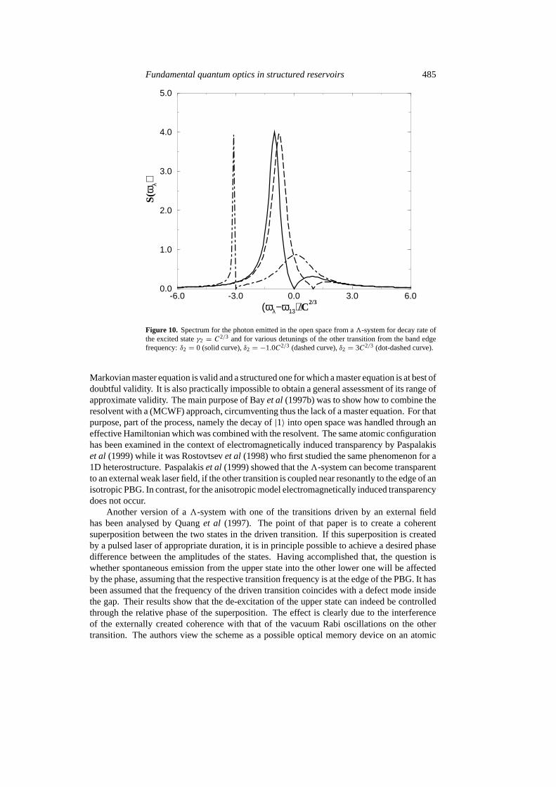
Fundamental quantum optics in structured reservoirs 485
-6.0 -3.0 0.0 3.0 6.0(ωλ−ω13)/C
2/3
0.0
1.0
2.0
3.0
4.0
5.0
S(ω
λ)
Figure 10. Spectrum for the photon emitted in the open space from a3-system for decay rate ofthe excited stateγ2 = C2/3 and for various detunings of the other transition from the band edgefrequency:δ2 = 0 (solid curve),δ2 = −1.0C2/3 (dashed curve),δ2 = 3C2/3 (dot-dashed curve).
Markovian master equation is valid and a structured one for which a master equation is at best ofdoubtful validity. It is also practically impossible to obtain a general assessment of its range ofapproximate validity. The main purpose of Bayet al (1997b) was to show how to combine theresolvent with a (MCWF) approach, circumventing thus the lack of a master equation. For thatpurpose, part of the process, namely the decay of|1〉 into open space was handled through aneffective Hamiltonian which was combined with the resolvent. The same atomic configurationhas been examined in the context of electromagnetically induced transparency by Paspalakiset al (1999) while it was Rostovtsevet al (1998) who first studied the same phenomenon for a1D heterostructure. Paspalakiset al (1999) showed that the3-system can become transparentto an external weak laser field, if the other transition is coupled near resonantly to the edge of anisotropic PBG. In contrast, for the anisotropic model electromagnetically induced transparencydoes not occur.
Another version of a3-system with one of the transitions driven by an external fieldhas been analysed by Quanget al (1997). The point of that paper is to create a coherentsuperposition between the two states in the driven transition. If this superposition is createdby a pulsed laser of appropriate duration, it is in principle possible to achieve a desired phasedifference between the amplitudes of the states. Having accomplished that, the question iswhether spontaneous emission from the upper state into the other lower one will be affectedby the phase, assuming that the respective transition frequency is at the edge of the PBG. It hasbeen assumed that the frequency of the driven transition coincides with a defect mode insidethe gap. Their results show that the de-excitation of the upper state can indeed be controlledthrough the relative phase of the superposition. The effect is clearly due to the interferenceof the externally created coherence with that of the vacuum Rabi oscillations on the othertransition. The authors view the scheme as a possible optical memory device on an atomic

486 P Lambropoulos et al
scale, which would be phase sensitive. Since Quanget al (1997) have chosen the frequency ofthe externally driven transition to be inside the gap, a defect mode was required for the driving.On the other hand Bayet al (1997), have chosen the analogous transition to be outside, inwhich case there is no need for a defect mode. That both arrangements are possible wouldbe of significance in the event an experimental implementation is ever attempted, as it wouldallow the driven frequency to be either larger or smaller than the one coupled to the edge, thusproviding further flexibility in the choice of the physical3-system.
Taking the driven transition far inside the gap, Quanget al (1997) have neglectedspontaneous emission, thus avoiding an open problem, namely multiple fluorescence of anexternally driven TLA at the edge of the gap. The MCWF method, as it has been developed inits Markovian formulation, can not describe the localization of photons at the site of the atom.The above limitation is connected with the nature of the MCWF technique and should alwaysbe kept in mind, as it can easily lead to pitfalls if extended beyond its range of validity. Acase in point is illustrated by the subsequent attempt of Quang and John (1997) to apply themethod to a case where more than one photon is present in the PBG reservoir by transformingto a dressed state basis, referring to the simulated state vectors as ‘dressed-state Monte Carlowavefunctions’. Their objective was to treat the problem of a TLA coupled to the PBG reservoirand at the same time driven by a laser. The difficulty in that treatment, in which they foundit necessary to neglect the coupling to the two-photon sector of the reservoir Hilbert spaceat one stage of their formal development, has been pointed out by Mølmer and Bay (1999).In Markovian MCWF, each time a jump occurs it is related to agedanken measurementofthe number of photons in the radiation reservoir (Dalibardet al 1992, Mølmeret al 1993).After each measurement the wavefunction of the system is projected on its zero- or one-photoncomponent and the photon in the latter case is annihilated by the detector. In PBG materials,however, the emitted photon(s) remain(s) localized at the site of the atom(s), leading thusto subsequent atomic reexcitation and population in higher sectors of the Hilbert space ofthe system (two-photon, three-photon, etc). Only photons with energy outside the gap canbe subject of such a measurement. The dubious validity of the treatment by Quang and John(1997) is shown to lead to unphysical spikes in the atomic population. The root of the difficultyis again related to the non-Markovian character of the process. One may ponder the possibilityof viewing the Quang and John (1997) treatment as an approximate technique, but for themoment it is far from evident how to evaluate the degree of approximation and thereforereliability.
5. Atom–atom interaction
We return now to the TLA and in this section we consider the mutual interaction between twoidentical TLAs. One of them is assumed to be in the upper state and the other in the lower. Forany mutual influence to be of any consequence in open space, the distance between the twoatoms must be of the order of the wavelength corresponding to the resonant transition fromthe upper to the lower state. Needless to say, the atoms must not be so close to each otheras to form a molecule or affect each other’s electronic states. The interaction must thus bemediated by the transverse photons of the dipole transition, the physical picture being that thephoton emitted by the excited atom is absorbed by the unexcited one, hence the term resonantdipole–dipole interaction (RDDI). At least in open space, that is the picture since the atomcannot reabsorb its own photon. Using the formalism of section 3, we should be able to givea quick but plausible derivation of a few simple equations, so as to provide the flavour ofthe calculations that are necessary for the quantitative treatment of the problem in differentreservoirs.

Fundamental quantum optics in structured reservoirs 487
If we label the atoms by A and B and the two states by|e〉 and |g〉, with |g〉 being thelower one, the relevant states of the problem are
|a〉 = |eA, gB, 0〉 (5.1)
|b〉 = |gA, eB, 0〉 (5.2)
|c〉 = |gA, gB, 1Ekq〉 (5.3)
with 1Ekq , indicating a photon of wavevectorEk and polarizationq. The position of the centreof mass of the atoms must also be included in the coupling to the radiation, which now reads
V = i∑j
∑Ekqµk[bEkqe
iEk ERj σ +j − b†
Ekqe−iEk ERj σ−j ] (5.4)
wherej = A,B andµk = (ωk/2ε0V )1/2Eεq Edeg with Edeg the electric dipole moment,ωk the
photon frequency andEεq the polarization vector. The interaction between the two atoms ismediated through state|c〉 which involves one photon in the reservoir. This means that theinteraction will be of second order inV having the form
Mab =∑c
VacVcb
z− ωc . (5.5)
This dipole–dipole matrix elementMab is in general complex and diverges as the interatomicdistance approaches zero. This is to be expected since in that limit a molecule is formed.Each of the atoms is of course directly coupled to the reservoir, which leads to the shift–widthfunction written in this case as∑
c
|Vjc|2z− ωc = 1− i0 (5.6)
being the same for both atoms andj = a, b. The shift1 can be assumed absorbed in theenergy of the upper state and with the lower state energy set equal to zero, the relevant matrixelements of the resolvent obey the equations
(z− ωa + i0)Gaa −MabGba = 1 (5.7a)
−MabGaa + (z− ωa + i0)Gba = 0. (5.7b)
The quantities0 represent the spontaneous decay widths of each atom. Assuming thatMab
has been replaced by az-independent quantity, the eigenvalues are given by
z± = ωa − i0 ±Mab. (5.8)
Substituted into the inversion integral, they lead to a damped sinusoidal behaviour in time.How strongly damped it is, depends on the atomic separation and strength of interaction inrelation to the decay rate0. In the long-time limit, however, the excited state population ineither atom will decay. The atoms may exchange excitation for a while, but they will eventuallyend up in the ground state.
The situation is basically similar if the atoms are inside a cavity in (near-)resonance witha mode. The equations for the matrix elements of the resolvent are in this case a bit morecomplicated (Bayet al 1997a) with three roots for the characteristic polynomial. All three arecomplex with dissipative parts, which means that again in the long-time limit all excitationis lost. The evolution in time is more involved because not only can the photon hop fromone atom to the other, but as we have seen in section 3, it can be reabsorbed by the sameatom. But the end result is the same; the atoms in the ground state and the cavity empty.Needless to say, the formal complication in going from open space to the cavity is due to theDOS which appear in all of the previous equations involving the summations overc, as these

488 P Lambropoulos et al
summations are converted to integrations. That includes the expression forMab. The algebraicmanipulations are analogous to those we have seen in section 3, but more of them. A recentdetailed treatment of this problem in a cavity has been presented by Goldstein and Meystre(1997). To the best of our knowledge, Kurizki (1990) was the first to ponder the extensionof RDDI to reservoirs of the type associated with PBG structures. The DOS he employeddiffered somewhat in the details from those currently in use, but the essential physics wasincluded. He has in fact considered several forms of DOS including some dissipation. Hisinterest in that paper was centred on the analytic structure of the RDDI termMab including itsimplications on quasimolecular collisions corresponding to small interatomic separationsR.He did not, however, study the implications on population trapping in the presence of RDDI,which can be anticipated on the basis of the behaviour of a TLA that we have seen in section 3.The issue of population trapping has been addressed more recently by Bayet al (1997a) whohave given first of all a rather detailed analysis of the behaviour of the RDDI as a function ofR. The DOS in the isotropic approximation has been used with particular emphasis on thebehaviour of the atom–atom coupling at the edge. This extends related work by John and Wang(1991) and Kweon and Lawandy (1994) who had studied the behaviour well inside the gap.The singular form of the DOS entails significant complexity in the calculation of the couplingMab. Among other aspects, it is necessary to consider in some detail the orientation of theatomic dipoles relative to the interatomic separation. Briefly, it turns out thatMab assumes theform
Mab =∑c
VacVcb
z− ωc = Vab −iCM√z− ωe (5.9)
whereVab denotes the term originating from the principal value part andCM (which can beassumed real) is given by
CM = ωe
4πε0
daegdbge
2√A
[k0 sin(k0R)
R+
cos(k0R)
R2− sin(k0R)
k0R3
](5.10)
obtained, as an example, for the two atomic dipoles parallel to each other butperpendicular toR. For atomic transitions outside the gap, i.e.z > ωe, the terminvolving CM gives an imaginary part toMab, while for z < ωe, Mab is real.Thus for frequencies inside the gap, the atom–atom interaction is dominated by theexchange of virtual photons, while for frequencies outside the gap,Mab contains adissipative part, which is different from the dissipative term involved in the couplingof each atom directly to the reservoir. That coupling in this situation is givenby ∑
c
|Vjc|2z− ωc = −
iCj√z− ωe (5.11)
where j = a, b. We have omitted the shift term in the above expression,assuming it will be incorporated in the energy of the state andCj is givenby
Cj = 1
4πε0
|deg|22√Ak2
0ωe2
3(5.12)
being the same forj = a or b. With the definition of states|a〉, |b〉 and |c〉 as given inequations (5.1)–(5.3), the matrix elementsGaa andGba of the resolvent are now found to obeythe equations[
z√z + δ + iC −√z + δVab + iCM
−√z + δVab + iCM z√z + δ + iC
] [Gaa
Gba
]=[√
z + δ0
](5.13)

Fundamental quantum optics in structured reservoirs 489
where to compress notation we have definedC = Ca = Cb, have introduced thetransformationz − ωa → z (i.e. interaction picture rotating atωa = ωb) and the detuningδ = ωa − ωe = ωb − ωe. This is the generalization of equations (5.7a), (5.7b) tothe case of the PBG reservoir. In arriving at equation (5.13) no pole approximationhas been introduced at any stage, as it is not allowed by the DOS. The unusualfeatures of the reservoir are reflected in the radicals appearing in the matrix of thecoefficients.
The eigenstates of the matrix in equation (5.13) can be readily identified as
|9s(a)〉 = 1√2
[|eA, gB〉 ± |gA, eB〉] (5.14)
which are the symmetric(s) and antisymmetric(a) product states. According to the currentvogue in terminology, these states correspond to entanglement of the two atoms. In open space,the symmetric state is known as a Dicke state which is unstable, leading to SR (see also thefollowing section). In the PBG reservoir, however, we can have excited population trappingeven in the symmetric state.
Much algebra and contour integration is required in order to proceed further. It can befound in Bayet al (1997a). We have now six roots which in the special case of negligibleVabhave a rather simple form. They are eiπ/3(C±CM)2/3, e−iπ/3(C±CM)2/3 and−(C±CM)2/3.The last two are real, and they are also roots of the original polynomial resulting from thedeterminant of the coefficients in equation (5.13). Obviously, they represent nondecayingstates of the system. But since we have two of them, the system has no true steady state, as itwill oscillate between these two nondecaying states. This behaviour is depicted in figure 11,for a particular choice of parameters. Note, however, that if the system is viewed in the basisof the the states|9s(a)〉 it is found to have a steady state. One of the real roots corresponding
0.0 10.0 20.0 30.0C
2/3 t
0.0
0.2
0.4
0.6
0.8
1.0
Ato
mic
Pop
ulat
ions
Figure 11. The time evolution of the excited state populations of two TLA, interacting throughRDDI at the edge of the PBG(δ = 0). The solid curve is for the initially excited atom (A) and thedashed curve for the initially unexcited atom (B). Parameters:CM = 0.5C,Vab = 0.

490 P Lambropoulos et al
0.0 5.0 10.0 15.0 20.0C
2/3t
0.0
0.2
0.4
0.6
0.8
1.0
0.2
0.4
0.6
0.8
1.0
Pop
ulat
ions
0.2
0.4
0.6
0.8
1.0(a)
(b)
(c)
Figure 12. The excited state population for the atom A (solid curve) and the total excitation in bothatoms (dot-dashed curve) as a function of time for(δ = −3C2/3), CM = 0.8C and for variousvalues ofVab: (a) Vab = 1C2/3, (b) Vab = 3C2/3, (c) Vab = 7C2/3.
to a stable (nondecaying) state is the eigenvalue of the symmetric product state, confirmingthus the assertion made above about the stability of the normally superradiant state.
The real partVab of Mab, becomes dominant for small interatomic separations (R � λ).For finiteVab andδ, the expressions for the roots become quite complicated (Bayet al1997a).The inversion integral can nevertheless be calculated numerically. Typical results, illustratingthe behaviour are shown in figure 12. For detuning sufficiently far inside the gap and smallVab(in units ofC2/3) there is almost complete population trapping, while for detuning outside thegap, the system decays with only a partial trapping which increases with the magnitude ofVab.The role ofVab in this effect is that it causes a splitting which, if comparable to the detuningfrom the edge, pushes part of the atomic levels into the gap for initially positive detuning andoutside the gap for initially negative detuning. This is what causes partial trapping for positivedetunings or partial decay for negative detuning, when in either caseVab is significantly largerthanC.
It is instructive to compare figure 13 with figure 2 where we have the time evolution ofthe upper state population of the TLA for various detunings from the edge. According tofigure 2, forδ = 3C2/3, the upper state population has practically decayed completely withina timet ≈ 5C−2/3. In figure 13, on the other hand, for the same detuning there is about 50%population trapping (25% for each atom) whenVab is equal to 5, i.e. less than a factor of 2larger than C. Thus RDDI has a stabilizing effect, even when the atomic frequency is outsidethe gap, which is in total contrast to the situation in open space where RDDI will always leadto decay. The strong coupling to the edge, which as we have seen causes the formation of thephoton–atom bound state, has the additional effect of binding two atoms into a stable state,

Fundamental quantum optics in structured reservoirs 491
0.0 5.0 10.0 15.0 20.0C
2/3t
0.0
0.2
0.4
0.6
0.8
1.0
0.2
0.4
0.6
0.8
1.0
Pop
ulat
ions
0.2
0.4
0.6
0.8
1.0(a)
(b)
(c)
Figure 13. The excited state population for the atom A (solid curve) and the total excitation inboth atoms (dot-dashed curve) as a function of time for(δ = 3C2/3), CM = 0.8C and for variousvalues ofVab: (a) Vab = 1C2/3, (b) Vab = 3C2/3, (c) Vab = 5C2/3.
although they are too far from each other to form a stable molecule.The distribution of the photonic population as a function of frequency is normally referred
to as the spectrum. In open space, the spectrum is given by the photonic distribution in thelong-time limit, as we have seen, for example, in the case of the ladder system. In the presentcontext, the issue is complicated by the fact that a detector located outside the (sufficientlylarge) photonic crystal, cannot detect the radiation wavepacket bound to and localized aroundthe atom. The photonic spectrum outside the gap does nevertheless reflect to some degree theinfluence of the strong coupling of the atomic transition to the edge. Relevant calculations forthe case of a TLA have been reported by Kofmanet al (1994) and for the case of two atoms byBayet al (1997a). Obviously, the spectrum does not contain frequencies corresponding to thegap and the contribution to the spectrum outside the gap represents radiation emitted duringthe transient regime before the photon–atom bound state is stabilized to its steady-state value.
The peculiarity in the issue of exploring the state of the radiation inside the photoniccrystal is not unique. It occurs in the micromaser (Weidingeret al1999), as it also does in anycavity QED experiment where information about the state of the radiation inside the cavityis obtained by interrogation of the exiting atom. An analogous arrangement for a photoniccrystal, however, does not seem easily feasible. In any case, it is interesting to keep in mindthe analogy of the two cases. Rather recently, the question of atom–atom dipole interactionand SR has also been investigated in the context of a microcavity at optical frequency (DeVoeand Brewer 1996).
The case ofN identical TLAs interacting only via RDDI, has been studied by John andQuang (1995b). The transition frequency for each TLA is assumed to be far inside the gap;

492 P Lambropoulos et al
Figure 14. Atomic population on the excited state of theinitially excited atom (a) and the unexcited atoms (b) as afunction of the scaled timeN1/2J t for detuning varianceδ = 0 and for different number of atoms:N = 10 (dottedcurves),N = 20 (solid curves),N = 30 (dashed-dottedcurves) andN = 40 (dashed curves). (John and Quang1995b.)
hence spontaneous emission can be neglected. Therefore the only interaction term in theHamiltonian, describing the RDDI between the atoms is of the form
∑i 6=j Jmnσ
+mσn, where all
constants and the dependence onER appearing in equation (5.4), have been included inJmn,which denotes the interaction between themth and thenth atom. The evolution of the systemcan then be determined by theN states|j〉 defined as|j〉 ≡ |g, g, . . . , e, g, . . . g〉 where thej th atom is excited. For an ordered system(Jmn = J ) and for large values ofN , the excitedatom does not transfer any excitation to the others. A disordered system was simulated bytaking Jmn as a Gaussian random variable with zero mean value and variance equal toJ .In this case, only a fraction of the initial excitation (proportional toN−1) can be transferredfrom the initially excited atom to each unexcited, with a rate of transfer proportional to
√N
(figure 14). If now all atoms are initially unexcited and near-resonant to a defect mode withsingle excitation, transfer of energy from the defect mode to the atoms does not occur for alarge ordered ensemble. By contrast, it does occur for a disordered system and the fraction ofthe defect excitation that is transferred to the atoms depends on the ratioJ/g whereg is thecoupling of each atom to the defect mode. Additionally, optical bistability, phase transitionsand collective atomic steady states are some of the phenomena that have been analysed in thecontext of theN TLAs interacting only via RDDI. The atoms are assumed to be coupled toa defect mode and can thus be driven by an external laser field. For a disordered system, theratio of the varianceJ to the Rabi frequency of the applied field (or the coupling to the defectmode), is of great importance in all of these phenomena, as has been pointed out by John andQuang (1996a, b, c).
6. Superradiance
When a collection ofN identical, initially excited atoms is confined in a volume withdimensions much smaller than the wavelength of the radiated lightλ, a cooperative effect,

Fundamental quantum optics in structured reservoirs 493
known as superradiance (SR) occurs. Spontaneous emission takes place in a timescale inverselyproportional to the number of radiated atoms, while the emission intensity is proportional toN2. This phenomenon was first discussed by Dicke (1954) in open space and since then ithas been attracting increasing interest. The superradiant behaviour is due to the induction ofcorrelations between the dipole moments of the initially uncorrelated atoms, that interact viaa common electromagnetic field (Allen and Eberly 1987, Andreevet al 1993). The emittedradiation, on the other hand, is characterized by a well defined directionality, depending on thegeometry of the sample. It could be said that SR is essentially a lasing phenomenon where theatoms have been pumped to their excited state att = 0. The resemblance of SR to laser physicswas the motivation for further investigation of superradiant schemes, from few to many atomsand from open space (Gross and Haroche 1987) to high-Q cavities (Haroche 1984, DeVoe andBrewer 1996). Thus it was to be expected that the appearance of PBG structures, that offer astrongly modified reservoir, would not fail to also attract attention in the context of SR.
Let us introduce at this point the Dicke notation, which is widely used in the literatureon SR (Gross and Haroche 1987). Assume a collection ofN identical TLAs, satisfying theprevious requirements, coupled near-resonantly to the edge of a PBG. Strictly speaking, thevolume in which the atoms are confined should not be arbitrarily small since, for atoms veryclose to each other, the dipole–dipole interaction between them leads to destruction of the SRbehaviour. Let also|a〉 and|g〉 be the upper and lower states for each of them. Att = 0, all ofthe atoms are excited and uncorrelated. For small times close tot = 0, SR is purely quantummechanical, since the atoms interact with the vacuum field until dipole–dipole correlationsarise. After this initial stage, however, the phenomenon becomes classical with a macroscopiccollection of dipoles emitting radiation in a way analogous to that of classical antennas. Sincethe atoms are confined in a volume with dimensions smaller thanλ, we can assume thatthe total dipole moment of the system is the sum over the dipole moments of individualatoms. Introducing the macroscopic atomic operatorsJ + = ∑
i |a〉ii〈g|, J− =∑
i |g〉ii〈a|,Jz =
∑i (|a〉ii〈a| − |g〉ii〈g|) the Hamiltonian of the complete system in RWA can be written
as
H = ω0Jz +∑k
ωka†kak +
∑k
µk(a†kJ− + akJ
+) (6.1)
whereµk =√
ωk2ε0VEεk · Ed with Ed being the dipole moment of the individual atom. The
macroscopic operators obey the well known commutation relations
[Jz, J±] = ±J±, [J +, J−] = 2Jz (6.2)
while we can define a complete set of orthogonal Dicke states|j,m〉 wherej = N2 and
mε[−j, j ] which are eigenstates ofJz andJ 2.There are mainly two ways of studying SR problems and both have been employed in
the literature. The first is the derivation of a Markovian master equation. There are, however,situations where the Born and Markov approximations are not valid, which invalidates the useof a master equation. PBG structures is definitely one of these situations and the alternativeis the solution of the Heisenberg equations of motion for the atomic and field operators. Johnand Quang (1994, 1995a) were the first to study SR at the edge of the gap in the context of theisotropic as well as the anisotropic model. This first work was followed by a second one (Vatsand John 1998) where the same question (SR at the edge of a PBG), was studied thoroughlyand in a somewhat broader context. In both cases, the problem was addressed by derivingHeisenberg equations of motion for the operators. In the Heisenberg picture, the equation ofmotion for an operatorA readsA ≡ −i[A, H ]. Following this definition and using (6.1), oneobtains the equations of motion for the field operators, the atomic inversionJz and the atomic

494 P Lambropoulos et al
polarizationJ−:
daλdt= −iωλaλ − iµλJ
− (6.3a)
dJzdt= i
∑λ
µλaλJ+ + h.c (6.3b)
dJ−
dt= −iω0J
− + 2i∑λ
µλaλJz (6.3c)
and after eliminating the field operators by formal integration, we have
d〈Jz〉dt= +
∫ t
0dt ′G(t − t ′)〈J +(t)J−(t ′)〉 + i〈ξ(t)J +(t)〉 + h.c. (6.4a)
d〈J−〉dt= −iδ〈J−(t)〉 + 2
∫ t
0dt ′G(t − t ′)〈Jz(t)J−(t ′)〉 + 2i〈ξ(t)Jz(t)〉 (6.4b)
where we have transformed to an interaction picture rotating at the band edge frequencyωe(δ = ω0 − ωe). We have in addition introduced the quantum noise operator
ξ(t) =∑λ
µλaλ(0)e−i(ωλ−ωe)t (6.5)
and the memory kernel (correlation) function of the reservoir
G(t − t ′) ≡ 〈ξ(t)ξ†(t ′)〉 =∑λ
µ2λe−i(ωλ−ωe)(t−t ′). (6.6)
As we have noted earlier, for open space the memory kernel is a delta function, reflecting theinstant loss of memory after the emission of a photon which never returns to the atom. For thecase of PBG materials and the isotropic model, the time correlations for the environment areof the form
GI(t − t ′) ∼ eiδ(t−t ′)√t − t ′ (6.7a)
while for the anisotropic model
GA(t − t ′) ∼ e−iδ(t−t ′)
(t − t ′)3/2 (6.7b)
with ωe(t − t ′)� 1 (Vats and John 1998).As we can see, the equations of motion (6.4a), (6.4b) do not constitute a closed set of
differential equations. On the contrary, they lead to other expectation values of higher-ordercorrelations, i.e.〈J +J−〉 and〈JzJ−〉. The resulting hierarchy of equations cannot be solved,unless it is somehow truncated. This truncation involves a decorrelation scheme and it isan approximation to the exact solution. There is no unique decorrelation approach, but thesimplest is the direct decorrelation of the products i.e.〈JzJ−〉 = 〈Jz〉〈J−〉, which is actually thefactorization adopted by John and collaborators. Following their approach, (6.4a) and (6.4b)can be written as follows:
d〈Jz〉dt= 2Re
{〈J +(t)〉
∫ t
0dt ′G(t − t ′)〈J−(t ′)〉
}(6.8a)
d〈J−〉dt= −iδ〈J−(t)〉 + 2〈Jz(t)〉
∫ t
0dt ′G(t − t ′)〈J−(t ′)〉 (6.8b)
where the average over the quantum noise has been set to zero(〈ξ(t)〉 = 0). From now on,we refer to these equations as mean-field (MF) equations. In figures 15 and 16 we present a

Fundamental quantum optics in structured reservoirs 495
0 10 20 30N
2/3 β 1t
�1
�0.5
0
0.5
1
<J 3
(t)>
/N
(a)
(b)
(c)
(d)
(e)
Figure 15. Mean field solution for the atomic inversion〈Jz(t)〉/N , near an isotropic PBG edgestarting with infinitesimal initial polarizationr = 10−5. Various values of the detuningδ from theband edge frequency: (a) δ = 1N2/3β1, (b) δ = 0.5N2/3β1, (c) δ = 0, (d) δ = −0.5N2/3β1,(e) δ = −1N2/3β1. (Vats and John 1998.)
sample of their results for the inversion and the polarization of a superradiant system at theedge of the gap and for the case of the isotropic model.
In open space it is well known that, in the long-time limit, all atoms are in the ground stateand thus there is no inversion or polarization. However, at the edge of the gap, the emittedradiation remains localized at the site of the atoms and thus the system exhibits steady-stateinversion and macroscopic polarization in the long-time limit, even for detunings outside thegap, as should have been anticipated from the behaviour of the TLA. Thus the ensemble ofthe atoms is finally inverted and it has a polarization with a constant amplitude, while thecorresponding phase angle changes with a constant rate. This clearly bears resemblance tothe coherence observed in a laser system. Both inversion and polarization exhibit oscillatorybehaviour instead of the exponential decay of open space. Nevertheless, it is noteworthythat the oscillations are not so pronounced in the anisotropic model, while there is neithersteady-state inversion nor macroscopic polarization, even for slight detunings of the atomictransition outside the gap. Although the behaviour of the ensemble has the main featuresof the single-atom behaviour at the edge of the gap, there is a crucial difference. For theensemble, the radiative lifetimeTc is shortened byN2/3 for the isotropic model and byN2 forthe anisotropic. Since the energy radiated by a collection ofN atoms isNhω0, the emissionintensity(I ≡ Nhω0/Tc) for the isotropic and the anisotropic model, is proportional toN5/3
andN3, respectively. Note that for open space the decay rate is proportional toN and theradiated intensity is proportional toN2. This means that the SR phenomenon at the edge ofthe gap for the anisotropic model is much faster and more intense than in open space, whilethe opposite is true for the isotropic model.

496 P Lambropoulos et al
0 10 20 30N
2/3 β 1t
0
0.1
0.2
0.3
0.4
0.5
0.6
0.7
0.8
<J
12(t
)>/N
(a)
(b)
(c)
(d)
(e)
Figure 16. Mean field solution for the atomic polarization amplitude|〈J−(t)〉|/N , near anisotropic PBG edge starting with infinitesimal initial polarizationr = 10−5. Various values ofthe detuningδ from the band edge frequency: (a) δ = 1N2/3β1, (b) δ = 0.5N2/3β1, (c) δ = 0,(d) δ = −0.5N2/3β1, (e) δ = −1N2/3β1. (Vats and John 1998.)
Having presented the main aspects of SR at the edge of the PBG, we return to theHeisenberg equations of motion and the decorrelation schemes. The factorization that wehave presented leads to a closed set of semiclassical equations for the expectation values ofthe inversion and the polarization. However the resulting set has an obvious mathematicaldrawback: if the system is initially fully excited, the system will never evolve, unless we givea nonzero initial value to the macroscopic polarization〈J−(0)〉. The semiclassical approachis valid for the description of the SR after the early stage, where the dipole correlations havealready been established and thus the evolution of the ensemble is purely classical. By contrast,the MF equations fail to recapture the influence of the vacuum (noise) at the early stage ofthe phenomenon, where the evolution is purely quantum mechanical. This aspect of thesemiclassical equations is of course well known in laser theory (Walls and Millburn 1994,Scully and Zubairy 1997).
This problem was the motivation for Bayet al (1998) to study SR in a Fano profileDOS, where a point gap exists for only a specific frequency. As we have noted earlier, theadvantage of this as well as of other models is that a Markovian master equation can be derived(Garraway 1997). Following Garraway’s approach on pseudomodes, Bayet al (1998) deriveda Markovian master equation for the Fano profile DOS, introducing two pseudomodes, one ofwhich was strongly damped. The atoms and the other pseudomode experienced dissipation viatheir coupling to this mode. The calculations, which need not be reproduced here, can be foundin Bay et al (1998) as well as Garraway (1997). The advantage now is that, having a masterequation, the validity of various decorrelation schemes can be tested, with respect to the exactsolution obtained by propagating the master equation. For a wide range of parameters, Bayet al

Fundamental quantum optics in structured reservoirs 497
(1998) have found that, at least for their model, the MF calculation gives very good agreementwith the exact calculation obtained from the master equation. This accuracy is, however,sensitive to the choice of the initial value assigned to the atomic operators. The best agreementis obtained if〈J−(0)〉 = √2j . Except for the MF approximation, another factorization schemewas also explored, namely the excitation conserving decorrelation, where expectation valuescontaining three operators are decorrelated, so that the resulting expectation values couplestates with the same number of excitation. We do not need to assign values by hand in this wayof decorrelation which gives good agreement with the exact calculation. In spite of the correctprediction of the atomic inversion in the long-time limit, both decorrelation schemes fail torecapture the early stage of SR, i.e. they overestimate the rapidity of the superradiant phase.This actually was also shown by Vats and John (1998). They pointed out that the choice of thetime t0 that determines the early-time atomic evolution regime, does not affect the steady-statevalue of〈Jz〉, but it does affect the onset time for the collective emission. Finally, we note thatfor the Fano profile gap model, Bayet al (1998) derived an analytic expression for the decayrate of the total number of excitations in the long-time limit, assuming a Gaussian distributionand applying perturbation theory.
7. Beyond one photon in the reservoir
The limitation of the approaches so far in handling only one photon in the structured reservoirwas noted in section 4. We know of no general remedy to this restriction. An approach thatcan at least partially overcome this stumbling block has been proposed and implemented ratherrecently by Nikolopouloset al (1999). The idea rests upon replacing the DOS by a sufficientlylarge set of discrete modes spaced appropriately so as to represent faithfully, but in a discretizedform, the analytical form of the DOS under consideration. This places some restrictions onthe height and spacing of modes, but there is flexibility in the details of the prescription. Acertain finite but large (say up to 500) number of modes can be accommodated depending oncomputational capability.
To illustrate how the method works, consider the TLA in its excited state as in section 3.Each mode is coupled to the atomic transition separately, through a coupling constant that isdetermined in the process of the discretization. This leads to a set of differential equations (asmany as the modes) governing the evolution of the system ‘atom +modes’. Within the numberof the modes included in the calculation, the treatment is practically exact. The success of theapproach depends on whether, for a given problem, the results can be shown to be insensitiveto further increase of the number of modes included in the calculation: the usual criterionfor convergence in any approach based on the discretization of a continuum. It turns out thatnumerical efficiency can in fact be increased significantly by introducing a further auxiliaryidea. It is based on the observation that modes sufficiently far from the edge can be eliminatedadiabatically giving rise to a shift, assuming of course as is usually the case, that the atomictransition is not too far from the edge, if it is taken outside the gap. It is the large detuningthat makes possible this elimination. In other words, distant modes are not coupled to theatom strongly. This realization suggests then a further improvement. We can keep the entireDOS, replace by a set of discretized modes only a part near the edge, and eliminate the restadiabatically. The application then to a specific problem is a matter of assessing which portionof the DOS needs to be discretized and how densely. This is part of testing the convergence ofthe calculation. The adiabatic elimination of distant (far detuned) frequencies illustrates certainqualitative aspects of the physics, namely the role of the distant modes in merely shifting theatomic transition further into the gap thus insulating it from decay.
When applied to the simple problem of section 3, the method is found to work quite well.

498 P Lambropoulos et al
0.0 10.0 20.0 30.0 40.0C
2/3t
0.0
0.5
1.0
1.5
2.0
Exc
itat
ions
Figure 17. The evolution of the system is plotted as function of time. The dotted curve is thepopulation in the upper atomic state. The solid curve is the mean photon number in the defectmode, the dot-dashed curve is the population in the one-photon sector of the reservoir Hilbertspace and the dashed curve is the population in the two-photon sector of the reservoir Hilbertspace. Parameters: number of discrete modesN = 150; coupling of the atom to the defect modegd = C2/3; detuning of the atomic transition for the band edge frequency and the defect mode’sresonant frequency10 = 1d = −0.1C2/3.
About 250 modes are sufficient to reproduce the results of figure 2, with an accuracy withinthe thickness of the lines of the curves. That simply represents a test that the method worksand is practical. Having established the soundness of the approach, we can go one step furtherto a problem involving two photons. Assume that we have a defect mode inside the gap anda TLA with transition frequency near or on resonance with the defect mode. Assume furtherthat att = 0 the defect mode carries the excitation of one photon and the TLA is in the excitedstate. The atom is thus coupled to both the defect mode and the PBG reservoir. To address thequestion of the time evolution of this system, we must consider states involving two photonsin the reservoir. The defect mode acts as a source that can pump the atom, which is in a way anintermediary between defect mode and the reservoir. The equations are now more complicatedthan the TLA alone, but can be readily handled with the approach outlined above. We shallforego a detailed description of the approach here, but we present one result pertaining to thisproblem. The calculation has been performed for the case of the defect mode on resonancewith the atomic transition and both somewhat past the edge inside the gap, i.e. detuning equal to−0.1C2/3. The isotropic approximation to the DOS has been assumed and 150 discrete modeswere required for convergence, a rather modest computational effort. The results depicted infigure 17 do contain a surprise, in that it could not have been anticipated on the basis of whatwe know from previous work. It shows radiation (photons) to be oscillating between defectmode and reservoir in a coherent fashion, while the atomic population remains constant, afteran initial transient period. And yet it is through the atom that the defect mode and reservoirexchange energy. The magnitude of this effect is fairly sensitive to the detuning from the edge.
Fundamental quantum optics in structured reservoirs 499
Thus we can now consider other problems where two photons are involved. For example,the ladder system with both transition frequencies inside the gap can be addressed and upondoing so, further surprises appear (Nikolopoulos and Lambropoulos 2000). A few morephotons can be also accommodated in the method. The limitation on the number of photonscomes from purely computational considerations, at least in the present form of the approach.What seems to emerge, on the basis of the glimpse we get into the few-photon extension of thephenomena we have been discussing, is that one or two more photons introduce considerablefurther richness in the behaviour of few-level systems coupled to these reservoirs.
8. Summary and outlook
The extension of the theory of cavity QED to PBG structures is by now well developed. Thefundamental effects are understood and a variety of arrangements involving few-levels atomswith frequencies around the band edge have been worked out and probably many more will. Itshould be clear that any problem posed in connection with atoms near resonance with isolatedcavity modes has its counterpart in a PBG structure, if the atom can be placed in it and asuitable way to monitor the desired effect can be arranged. In this respect it is useful to keepin mind that in most if not all cavity–atom physics, the atoms stream through the cavity andthe information on the outcome of the interaction is obtained by monitoring the state of theexiting atom. Although problems assuming the same procedure with photonic crystals havebeen addressed (Kurizkiet al 1993) it is not clear how it could be implemented. That beingas it may, the fundamental difference between a high-Q cavity and an ideal PBG crystal isencapsulated in the behaviour of the TLA. In the cavity, it will decay to the lower state in thelong-time limit while a fraction of the population will remain trapped for a transition frequencyinside the gap. According to the models adopted in the calculations, the trapping lasts ‘forever’.In reality of course photonic crystals have losses as well, which will depend on the material,geometry, size, etc. As of now, quality factors of the order of 104–105 have been estimated frommeasurements of attenuation (Linet al 1996), while John (1994) places theoretical estimatesas high as 1010. A state-of-the-art superconducting niobium cavity at microwave frequenciescurrently in use for quantum optics experiments hasQ of the order 3× 10¹⁰. Even with suchhighQ, the vacuum Rabi frequency for Rydberg atoms is larger than the photon damping ratebut not much larger. The DOS and the mode structure of a photonic crystal have, on the otherhand, different forms which are expected to provide stronger coupling. Thus for the sameQ,the vacuum Rabi frequency in a photonic crystal may be appreciably larger than in a cavity.One of the most interesting aspects of photonic crystals is the flexibility in designing the spatialform of the vector potential.
The basic effect of population trapping in the TLA, as we have seen, carries over tomore complicated arrangements with more levels or more atoms, or both. One rather startlingconsequence, for example, is the stabilization of the Dicke superradiant state. The drive forthe development of photonic crystals comes from technological demands mentioned earlierin section 2 and not from quantum optics. Yet many technological aspects such as opticalswitches, for example, are related to those of interest in quantum optics; especially if viewedin a broader context where the ‘atom’ is replaced by a p–n junction as in LEDs. In the fewexperimental tests of inhibition of spontaneous emission, the two-level ‘atoms’ in reality wereeither dye molecules (Petrovet al 1998, Megenset al 1999) or LED (Tocciet al 1996), allpermanently fixed in the structure. Exploring experimentally all these other effects beyond the‘TLA’ will not be a straightforward task.
Hopefully, there will be further much needed experimental exploration of the many effectsfor which the theory has been worked out. When it comes to the point of comparing theory

500 P Lambropoulos et al
with experiment, more realistic DOS, pertaining to each case will be needed. Most of thecalculations so far have relied on the isotropic approximation to the DOS. Far inside the gapthe predictions may not change much but, at the edge and even slightly beyond, the behaviourwould be modified drastically.
In fact, a rather serious consequence of the isotropic DOS is the significant amount ofpopulation trapping even for atomic transition frequencies outside the gap, as we have seen,for example, in figures 2 and 13. This can be traced to the fact that the DOS drops ratherprecipitously beyond the edge outside the gap. In some sense, this acts as a pseudo-gap outsidethe main gap. On the other hand, this population trapping for positive detuning is totally absentin the anisotropic model where the DOS does not exhibit a drop outside the gap. It is thusdoubtful that population trapping and related effects would exist under realistic conditions forpositive detuning. It would of course be nice if such effects did exist as they would provide ahandle for detecting the effects of the gap by examining radiation of frequency outside the gapwhich can propagate through the photonic crystal. Such a handle could possibly be introducedthrough a defect mode at an appropriate frequency inside the gap.
A beneficial side-effect of the quantum optics issues in photonic crystals has been theinquiry into techniques for handling non-Markovian processes (Diosi et al 1998, Strunzet al1999). This combined with the breakdown of the Born approximation in the master equationhas led to the formulation of mathematical issues that reach beyond the particular application toPBG structures. If significant progress is made along those lines, the dividend on the investmentin these investigations will have been worthwhile, with impact in a broader context.
We should not close without pointing out the connection with optical lattices. Thepossibility of a photonic gap in an optical lattice of laser-cooled atoms was explored fairlyearly by Deutschet al (1995) who showed the existence of a gap in two dimensions. Morerecently, van Coevordenet al (1996) and Spriket al (1996) have argued that a full 3D gapshould exist in an optical lattice. The calculation treats the atoms of the lattice as point dipoleswith damping and it is Bragg scattering by the periodic array of such dipoles that causesthe gap. Bragg scattering from atomic lattices has already been observed (Weidemuller et al1995). The gap is around the resonance atomic frequency. One limitation at the time of thework by Coevordenet al (1996) was the low filling factor ('15%) of such lattices. In themeantime much progress has been made on that issue (DePueet al 1999). Moreover, with therapid development of Bose–Einstein condensates, it should be possible to fill such lattices. Alimitation in the treatment of (Coevordenet al 1996) was the neglect of the oscillatory motionof the atoms around the equilibrium position. This can be accounted for, through a Debye–Waller factor, with the net effect expected to be a reduction in the Bragg-scattered intensity.It is not clear how large the gap can be. Moreover the size of the lattice itself, being limitedby the diameter of the laser beams, is apt to be rather small. Thus it remains to be establishedhow large and how ‘good’ the gap can be. Assuming things can be optimized, the possibilitiesfor the type of questions discussed in the previous sections are quite intriguing in an opticallattice. It may well be that atoms could stream through such a lattice as they do in a cavity.
References
Abram I and Bourdon G 1996Phys. Rev.A 543476Agarwal G S 1974Quantum Statistical Theories of Spontaneous Emission and their Relation to other Approaches
(Springer Tracts in Modern Physics vol 70)(Berlin: Springer)Allen L and Eberly J H 1987Optical Resonance and Two-Level Atoms(New York: Dover)An K, Childs J J, Dasari R R and Feld M S 1994Phys. Rev. Lett.733375Andreev A V, Emel’yanov V I and Il’inskii Yu A 1993 Cooperative Effects in Optics: Superradiance and Phase
Transitions (Malvern Physics Series)ed E R Pike (Bristol: Institute of Physics Publishing)
Fundamental quantum optics in structured reservoirs 501
Bay S 1998PhD ThesisInstitute of Physics and Astronomy, University of AarhusBay S and Lambropoulos P 1998Opt. Commun.146130Bay S, Lambropoulos P and Mølmer K 1997aPhys. Rev.A 551485——1997bPhys. Rev. Lett.792654——1998Phys. Rev.A 573065Bendickson J M, Dowling J P and Scalora M 1996Phys. Rev.E 534107Bogomolov V N, Gaponenko S V, Kapitonov A M, Prokofiev A V, Ponyavina A N, Silvanovich N I and Samoilovich S M
1996Appl. Phys.A 63S613–6Coevorden D V, Sprik R, Tip A and Lagendijk A 1996Phys. Rev. Lett.772412Cohen-Tannoudji C, Dupont-Roc J and Grynberg G 1992Atom–Photon Interactions(New York: Wiley)Curtis S 1999Vacuum SolutionsMay/June 19Dalibard J, Castin Y and Mølmer K 1992Phys. Rev. Lett.68580DePue M T, McCormick C, Winoto S L, Oliver S and Weiss D S 1999Phys. Rev. Lett.822262Deutsch I H, Spreeuw R J C,Rolston S L and Philips W D 1995Phys. Rev.A 521394DeVoe R G and Brewer R G 1996Phys. Rev. Lett.762049Dicke R H 1954Phys. Rev.9399Diosi L, Gisin N and Strunz W T 1998Phys. Rev.A 581699Dobiasch P and Walther H 1985Ann. Phys., Paris10825Dowling J P and Bowden C M 1992Phys. Rev.A 46612——1993J. Opt. Soc. Am.10353Dowling J P, Scalora M, Bloemer M J and Bowden C M 1994J. Appl. Phys.751896Fano U 1961Phys. Rev.1241866Fogel I S, Bendickson J M, Tocci M D, Bloemer M J, Scalora M, Bowden C M and Dowling J P 1998Pure Appl. Opt.
7 393Garraway B M 1997Phys. Rev.A 552290Giessen H, Berger J D, Mohs G, Meystre P and Yelin S F 1996Phys. Rev.A 532816Gisin N and Percival I C 1992J. Phys. A: Math. Gen.255677——1993aJ. Phys. A: Math. Gen.262233——1993bJ. Phys. A: Math. Gen.262245Goldberger M L and Watson K M 1964Collision Theory(New York: Wiley)Goldstein E V and Meystre P 1997Phys. Rev.A 565135Gross M and Haroche S 1982Phys. Rep.93301Haroche S 1984In New Trends in Atomic Physicsed G Grynberg and R Stora (Amsterdam: Elsevier)——1992Fundamental Systems in Quantum Opticsed J Dalibard, J M Raimond and J Zinn-Justin (Amsterdam:
North-Holland)Hansch T W and Walther H 1999Rev. Mod. Phys.71S242Hinds E A 1991Advances in Atomic Molecular and Optical Physicsvol 20, ed D Bates and B Bederson (New York:
Academic) p 237Ho K M, Chan C T and Soukoulis C M 1990Phys. Rev. Lett.653152Huang H, Lu X H and Zhu S Y 1998Phys. Rev.A 574945Imamoglu A 1994Phys. Rev.A 503650Joannopoulos J D 1995Photonic Crystals: Molding the Flow of Light(Princeton, NJ: Princeton University Press)Joannopoulos J D, Villeneuve P R and Fan S 1997Nature386143John S 1987Phys. Rev. Lett.582486——1991Phys. Today(May) 32——1997Nature390662——1994Confined Electrons and PhotonsNATO ASI (London: Plenum)——1994Photonic Band Gap MaterialsNATO ASI (Dordrecht: Kluwer)John S and Wang J 1990Phys. Rev. Lett.642418——1991Phys. Rev.B 4312 772John S and Quang T 1994Phys. Rev.A 501764——1995aPhys. Rev. Lett.743419——1995bPhys. Rev.A 524083——1996aPhys. Rev. Lett.762484——1996bPhys. Rev.A 544479——1996cPhys. Rev. Lett.761320——1997aPhys. Rev. Lett.781888——1997bPhys. Rev.A 564273

502 P Lambropoulos et al
Kamli A, Babiker M, Al-Hajry A and Enfati N 1997Phys. Rev.A 551454Kili n S Y and Mogilevtsev D S 1992Laser Phys.2 153——1993Opt. Spectrosc.74579Kitson S C, Barnes W L and Sambles J R 1996Phys. Rev. Lett.772670Kleppner D 1981Phys. Rev. Lett.47233Kofman A G, Kurizki G and Sherman B 1994J. Mod. Opt.41353Kurizki G 1990Phys. Rev.A 422915Kurizki G, Sherman B and Kadyshevitch A 1993J. Opt. Soc. Am.10346Kweon G I and Lawandy N M 1994J. Mod. Opt.41311Levi B G 1999Phys. Today(January) 17Lewenstein M, Zakrzewski J and Mossberg T W 1988aPhys. Rev.A 38808Lin H-B, Tonucci R J and Campillo A J 1998Opt. Lett.2394Lin S-Y, Hietala V M, Lyo S K and Zaslavsky A 1996Appl. Phys. Lett.683233Lin S-Y, Fleming J G, Sigalas M M, Biswas R and Ho K M 1999Phys. Rev.B 59R15 579Louisell W H 1990Quantum Statistical Properties of Light(New York: Wiley)Maitre X, Hagley E, Nogues G, Wunderlich C, Goy P, Brune M, Raimond J M and Haroche S 1997Phys. Rev. Lett.
79769Martorell J and Lawandy N M 1990Phys. Rev. Lett.651877Megens M, Wijnhoven J E G J,Lagendijk A and Vos W L 1999Phys. Rev.A 594727Meystre P 1992Progress in Opticsvol 30, ed E Wolf (Amsterdam: Elsevier) p 261Meystre P and Sargent M 1999Elements of Quantum Optics(Berlin: Springer)Marrocco M, Weidinger M, Sang R T and Walther H 1998Phys. Rev. Lett.815784Mossberg T W and Lewenstein M 1993J. Opt. Soc. Am.10340Mølmer K and Bay S 1999Phys. Rev.A 59904Mølmer K, Castin Y and Dalibard J 1993J. Opt. Soc. Am.10524Moy G M, Hope J J and Savage C M 1999Phys. Rev.A 59667Moy G M and Savage C M 1997Phys. Rev.A 56R1087Nabiev R F, Yeh P and Sanchez-Mondragon J J 1993Phys. Rev.A 473380Nikolopoulos G M, Bay S and Lambropoulos P 1999Phys. Rev.A 605079Nikolopoulos G M and Lambropoulos P 2000Phys. Rev.A to be publishedPaspalakis E, Kylstra N J and Knight P L 1999Phys. Rev.A 60R33Petrov E P, Bogomolov V N, Kalosha I I and Gaponenko S V 1998Phys. Rev. Lett.8177Plenio B M and Knight P L 1998Rev. Mod. Phys.70101Quang T and John S 1997Phys. Rev.A 564273Quang T, Woldeyohannes M, John S and Agarwal G S 1997Phys. Rev. Lett.795238Raithel G, Wagner C, Walther H, Narducci L M and Scully M O 1994Advances in Atomic Molecular and Optical
Physicsed P R Berman (New York: Academic) p 57 (suppl. 2)Rempe G, Schmidt-Kaler F and Walther H 1990Phys. Rev. Lett.642783Rostovtsev Y V, Matsko A B and Scully M O 1998Phys. Rev.A 574919Sakurai J J 1995Advanced Quantum Mechanics(New York: Addison-Wesley)Sargent M, Scully M O and Lamb W E Jr1974Laser Physics(Reading, MA: Addison-Wesley)Scalora M, Dowling J P, Bowden C M and Bloemer M J 1994aJ. Appl. Phys.762023——1994bPhys. Rev. Lett.731368Scalora M, Dowling J P, Tocci M, Bloemer M J, Bowden C M and Haus J W 1995Appl. Phys.B 60S57–61Scalora M, Flunn R J, Reinhardt S B, Fork R L, Bloemer M J, Tocci M D, Bowden C M, Ledbetter H S, Bendickson J M
and Leavitt R P 1996Phys. Rev.E 54R1078Scully M O and Zubairy M S 1997Quantum Optics(Cambridge: Cambridge University Press)Sherman B, Kofman A G and Kurizki G 1995Appl. Phys.B 60S99–105Shore B 1990The Theory of Coherent Excitation(New York: Wiley)Sprik R, Tiggelen B A and Lagendijk A 1996Europhys. Lett.35265Stanley R P, Houdre R, Oesterle U, Ilegems M and Weisbuch C 1993Phys. Rev.A 482246Steane A 1998Rep. Prog. Phys.61117Stenius P and Imamoglu A 1996Quantum Semiclass. Opt.8 283Strunz W T, Diosi L and Gisin N 1999Phys. Rev.A 821801Tocci M D, Bloemer M J, Scalora M, Dowling J P and Bowden C M 1995Appl. Phys. Lett.662324Tocci M D, Scalora M, Bloemer M J, Dowling J P and Bowden C M 1996Phys. Rev.A 532799Vats N and John S 1998Phys. Rev.A 584168Villeneuve P R, Fan S and Joannopoulos J D 1996Phys. Rev.B 547837
Fundamental quantum optics in structured reservoirs 503
Visser P M and Nienhuis G 1997Opt. Commun.136470Vos W L, Sprik R, Blaaderen A, Imhof A, Lagendijk A and Wegdam G H 1996Phys. Rev.B 5316 231Walls D F and Milburn G J 1994Quantum Optics(Berlin: Springer)Walther H 1992Phys. Rep.219263–81Wanke M C, Lehmann O, Muller K, Wen Q and Stuke M 1997Science2751284Weidemuller M, Hemmerich A, Gorlitz A, Esslinger T and Hansch T W 1995Phys. Rev. Lett.754583Weidinger M, Varcoe B T H,Heerlein R and Walther H 1999Phys. Rev. Lett.823795Weiss M 1993Quantum Dissipative Systems(Singapore: World Scientific)Wijnhoven J E G j and Vos W L1998Science281802Yablonovitch E 1987Phys. Rev. Lett.582059Yablonovitch E, Gmitter T J and Leung K M 1991bPhys. Rev. Lett.673380Yablonovitch E, Gmitter T J, Meade R D, Brommer K D, Rappe A M and Joannopoulos J D 1991aPhys. Rev. Lett.
672295Yamamoto Y and Slusher R S 1993Phys. Today4666Zhu S Y, Chen H and Huang H 1997Phys. Rev. Lett.79205Zi J, Wan J and Zhang C 1998Appl. Phys. Lett.732084