Functions of a Complex Variable(Zill & Wright Chapter 17)

1016-420-02: Complex Variables∗

Fall 2011

Contents

0 Administrata 20.1 Outline . . . . . . . . . . . . . . . . . . . . . . . . . . . . . . . . . . . . . . . 3

1 Complex Numbers 3

2 The Complex Plane 62.1 Polar Form of a Complex Number . . . . . . . . . . . . . . . . . . . . . . . . 72.2 Roots and Powers of a Complex Number . . . . . . . . . . . . . . . . . . . . 82.3 Regions in the Complex Plane . . . . . . . . . . . . . . . . . . . . . . . . . . 12

3 Functions of a Complex Variable 143.1 Complex Functions . . . . . . . . . . . . . . . . . . . . . . . . . . . . . . . . 14

3.1.1 Visualizing Complex Functions . . . . . . . . . . . . . . . . . . . . . 143.2 Complex Differentiation . . . . . . . . . . . . . . . . . . . . . . . . . . . . . 183.3 The Cauchy-Riemann Equations . . . . . . . . . . . . . . . . . . . . . . . . . 21

3.3.1 The Fine Print: Differentiable vs Analytic . . . . . . . . . . . . . . . 223.3.2 Aside: Vector Calculus . . . . . . . . . . . . . . . . . . . . . . . . . . 233.3.3 Harmonic Functions . . . . . . . . . . . . . . . . . . . . . . . . . . . 24

3.4 Some Specific Functions . . . . . . . . . . . . . . . . . . . . . . . . . . . . . 263.4.1 Exponentials, Logarithms and Powers . . . . . . . . . . . . . . . . . . 273.4.2 Trigonometric and Hyperbolic Functions . . . . . . . . . . . . . . . . 33

A Taylor Series and the Euler Relation 37

∗Copyright 2011, John T. Whelan, and all that

1

Tuesday 6 September 2011

0 Administrata

• Syllabus

• The last letter of the English alphabet, z, can be pronounced “zee” or “zed”, dependingon your dialect.

• Instructor’s name (Whelan) rhymes with “wailin’”.

• Text: Zill and Wright, Advanced Engineering Mathematics. You’ll need to sign upfor WebAssign access, but note that this can be purchased separately from the book.WebAssign makes the sections of the book available online, but unfortunately not theExercises, which are used for practice problems. There is a copy of the book on reserveat the Library.

• Course website: http://ccrg.rit.edu/~whelan/1016-420/

• Course calendar: tentative timetable for course.

• Structure:

– Read relevant sections of textbook before class

– Lectures to reinforce and complement the textbook

– Practice problems (odd numbers; answers in back but more useful if you try thembefore looking!).

– In-class exercises and simple quizzes; intended either to check basic concepts fromassigned reading, or to emphasize ideas through active learning.

– Weekly homework via WebAssign.

∗ Note: doing the problems is very important step in mastering the material.

∗ Note that you get 100 tries for each non-multiple-choice question, so youshould be able to get most or all correct with sufficient effort.

∗ In addition, you can earn 10% extra credit on a problem set by turning in acomplete, neatly handwritten solution to your WebAssign problems, due atthe beginning of class on the due date. This is useful practice for the exams!

∗ Most of the questions are based on the “Review Questions” at the end ofeach chapter. The odd-numbered review questions have answers in the backof the book, but note that the WebAssign versions have had some numberschanged.

∗ Numbers in the questions are “randomized” so that each student will get aslightly different version of the same problem, and therefore a different rightanswer!

– Prelim exam (think midterm, but there are two of them) in class at end of each halfof course: closed book, one handwritten formula sheet, use scientific calculator(not your phone!)

– Final exam to cover both halves of course

2

• Grading:

5% In Class Exercises/Quizzes

10% Problem Sets

25% First Prelim Exam

25% Second Prelim Exam

35% Final Exam

You’ll get a separate grade on the “quality point” scale (e.g., 2.5–3.5 is the B range)for each of these five components; course grade is weighted average.

0.1 Outline

Part One:

• Functions of a Complex Variable (Chapter 17)

• Integration in the Complex Plane (Chapter 18)

Part Two:

• Series and Residues (Chapter 19)

• Conformal Mappings (Chapter 20)

1 Complex Numbers

Ordinary numbers found on the number line, like 1, 42, 0, −12, 1.25, π, −13,√

2, arecalled real numbers. The set of all real numbers is called R and it includes as subsetsrational numbers, irrational numbers, integers, positive numbers, negative numbers, etc.When working with real numbers, we can add, subtract, multiply, and divide them (exceptdivision by zero) and the result is another real number. But we cannot solve an equation likex2 + 1 = 0, because there is no real number whose square is −1. So we invent a new numbercalled i, defined by i2 = −1.1 We can then construct numbers of the form z = x+ iy, wherex and y are both real numbers.2 (I.e., x, y ∈ R.) Such numbers are called complex numbers,and the set of all complex numbers is called C. This course will be concerned with complexfunctions of complex numbers, i.e. functions of the form w = f(z), where w, z ∈ C. Theresulting field of Complex Analysis will allow us to solve problems involving real functions,and have numerous applications in science and engineering.

But first we will consider the algebra of complex numbers. It turns out that if you add,subtract, multiply and divide complex numbers (except division by 0 = 0 + 0i), the resultwill always be a complex number; by applying i2 = −1 you can always get it back into the

1In some engineering textbooks, this number is called j; other less common notations are I and even J .In python, it is written 1j.

2Another possible notation for z = x+ iy is (x, y); we won’t typically use this in algebraic formulas, butit’s useful to keep in mind for e.g., representing complex numbers on a computer.

3

form x + iy, where x and/or y may be negative or zero. We can write down “rules” forthis, but in fact most of it follows from the extension of standard algebra and application ofi2 = −1. So you can work out some of these operations in the following exercise:

In-class exerciseHere are the general formulas for the operations you’ve carried out:

• Addition:(x1 + iy1) + (x2 + iy2) = (x1 + x2) + i(y1 + y2) (1.1a)

• Subtraction:(x1 + iy1)− (x2 + iy2) = (x1 − x2) + i(y1 − y2) (1.1b)

• Multiplication:

(x1+iy1)(x2+iy2) = x1x2+i(x1y2+y1x2)+i2y1y2 = (x1x2−y1y2)+i(x1y2+y1x2) (1.1c)

Note that (x + iy)(x − iy) = x2 − (iy)2 = x2 − (−1)y2 = x2 + y2 which is a positivereal number (unless x = 0 = y, in which case it’s zero).

• Division:

x1 + iy1

x2 + iy2

=

(x1 + iy1

x2 + iy2

)(x2 − iy2

x2 − iy2

)=

(x1 + iy1)(x2 − iy2)

(x2)2 + (y2)2

=(x1x2 + y1y2) + i(−x1y2 + y1x2)

(x2)2 + (y2)2=

x1x2 + y1y2

(x2)2 + (y2)2+ i−x1y2 + y1x2

(x2)2 + (y2)2

(1.1d)

Note that in practice no one memorizes (or even looks up) (1.1d); we just apply thetrick of multiplying and dividing by x2− iy2 whenever we have a fraction with x2 + iy2

in the denominator.

Another useful fact is that (−i)2 = (−1)2i2 = i2 = −1. This means that in some sense iand −i are on the same footing as square roots of −1. Because of this fact, an interestingoperation is the complex conjugate, which switches i and −i. The complex conjugate of acomplex number z is written3 z and is defined as

z = x+ iy = x− iy (1.2)

The two real numbers which are equivalent to a complex number z = x+ iy are the realpart Re(z) = x and the imaginary part Im(z) = y. Note that the imaginary part of z is areal number! We can also write these using the complex conjugate:

z + z

2=

(x+ iy) + (x− iy)

2= x = Re(z) (1.3a)

z − z2

=(x+ iy)− (x− iy)

2i= y = Im(z) (1.3b)

3In many applications, typically outside of complex analysis courses, the complex conjugate is written z∗

instead of z.

4

Another handy fact is that i(−i) = −i2 = −(−1) = 1. This is part of the reason that, asnoted before,

zz = (x+ iy)(x− iy) = x2 + y2 (1.4)

which is a non-negative real number. This is the square of what we call the modulus

|z| =√zz =

√x2 + y2 (1.5)

The modulus is the complex generalization of the absolute value. Note that if y = 0 (so thatz is the real number x), the modulus is

√x2 = |x|.

We can perform most of the same operations and manipulations on complex numbersthat we can on real numbers. Two notable exceptions:

• There is no concept of one complex number being greater than or less than another.While equality and inequality are well defined:

x1 + iy1 = x2 + iy2 iff x1 = x2 and y1 = y2 (1.6a)

x1 + iy1 6= x2 + iy2 iff x1 6= x2 or y1 6= y2 , (1.6b)

the symbols >, <, ≥, and ≤ have no meaning when applied to complex numbers.

• We only know how to take the square root of a non-negative real number. The symbol√

will never ever ever be applied to anything but a non-negative real number.

We will instead use fractional powers, so for example w = z1/2 means that w is anynumber such that w2 = z. For example, we’ve seen that i2 = −1 = (−i)2, so we knowthat

(−1)1/2 = i or − i (1.7)

The expression z1/2 is not single-valued. (In fact, we’ll see that if z 6= 0, there areexactly two possible values for z1/2.) Note that this also applies to positive numbers.For example, 22 = 4 = (−2)2 so

41/2 = 2 or − 2 . (1.8)

Similarly,21/2 =

√2 or −

√2 . (1.9)

Note the distinction.√

2 is the single positive number 1.414 . . ., while 21/2 is multi-valued, and can be

√2 or −

√2.

Exercise: What is i1/2? I.e., what are the possible combinations of x and y so that

(x+ iy)2 = (x+ iy)(x+ iy) = i ? (1.10)

Practice Problems

17.1.1, 17.1.5, 17.1.9, 17.1.13, 17.1.15, 17.1.27, 17.1.35, 17.1.39

5

Thursday 8 September 2011

Handy table:

θ −5π/6 −3π/4 −2π/3 −π/2 −π/3 −π/4 −π/6θ(360◦/2π) −150◦ −135◦ −120◦ −90◦ −60◦ −45◦ −30◦

sin θ −1/2 −√

2/2 −√

3/2 −1 −√

3/2 −√

2/2 −1/2

cos θ −√

3/2 −√

2/2 −1/2 0 1/2√

2/2√

3/2

θ 0 π/6 π/4 π/3 π/2 2π/3 3π/4 5π/6 π

θ(360◦/2π) 0◦ 30◦ 45◦ 60◦ 90◦ 120◦ 135◦ 150◦ 180◦

sin θ 0 1/2√

2/2√

3/2 1√

3/2√

2/2 1/2 0

cos θ 1√

3/2√

2/2 1/2 0 −1/2 −√

2/2 −√

3/2 −1

2 The Complex Plane

Recall that a complex number z = x+ iy can also be thought of as the ordered pair of realnumbers (x, y). It is useful to associate the complex number z = x+ iy with the point withCartesian coordinates (x, y). Each complex number can then be thought of as a point in the“complex plane” with the corresponding coordinates.

6

2.1 Polar Form of a Complex Number

An alternative to Cartesian coordinates (x, y) which is often useful is polar coordinates (r, θ),defined by

x = r cos θ (2.1a)

y = r sin θ (2.1b)

In terms of the polar coordinates (r, θ), the complex number is

z = (r cos θ) + i(r sin θ) = r(cos θ + i sin θ) = reiθ (2.2)

In the last step, we have used the Euler Relation

eiθ = cos θ + i sin θ (2.3)

which follows from the Taylor series for the sine, cosine and exponential functions, as shownin detail in Appendix A. Some useful examples:

ei0 = cos 0 + i sin 0 = 1 + i0 = 1 (2.4a)

eiπ/2 = cosπ

2+ i sin

π

2= 0 + i1 = i (2.4b)

eiπ = cosπ + i sin π = −1 + i0 = −1 (2.4c)

e−iπ/2 = cos(−π

2

)+ i sin

(−π

2

)= 0 + i(−1) = −i (2.4d)

2eiπ/4 = 2(

cosπ

4+ i sin

π

4

)= 2

(√2

2+ i

√2

2

)=√

2 + i√

2 (2.4e)

By the Pythagorean theorem, the radial coordinate r is the modulus of the complexnumber z

r =√x2 + y2 =

√zz = |z| (2.5)

The angular coordinate θ is called the argument of z. Note that, because cos θ and sin θare periodic with period 2π, there are many choices of θ which give z = reiθ. For example,ei3π/2 = −i = e−iπ/2 and ei2π = 1 = ei0. This multi-valued argument is written “arg”:

arg z = θ : z = |z| eiθ = |z| (cos θ + i sin θ) (2.6)

For example,

arg i = . . . or − 3π

2or

π

2or

5π

2or . . . =

{ π2

+ k 2π∣∣∣ k ∈ Z

}(2.7)

For any z there is a choice of θ = arg z such that −π < θ ≤ π. We call this the principalvalue of the argument and write it Arg z:

Arg z = atan2(y, x) =

Arctan(y/x)− π x < 0 and y < 0

−π/2 x = 0 and y < 0

Arctan(y/x) x > 0

π/2 x = 0 and y > 0

Arctan(y/x) + π x < 0 and y ≥ 0

(2.8)

7

The value of Arg z divides the complex plane into quadrants:

Note that Arg z is discontinuous on the negative real axis; Arg(−1) = π, but Arg(−1+ iε) ≈−π + ε for small positive ε.

Recall that the complex conjugate of z = x+ iy is z = x− iy. If we write z in polar form

z = reiθ = (r cos θ) + i(r sin θ) (2.9)

its complex conjugate is

z = (r cos θ) + i(−r sin θ) = r cos(−θ) + ir sin(−θ) = re−iθ (2.10)

I.e.,

|z| = |z| (2.11a)

arg(z) = − arg(z) (2.11b)

Question: is Arg(z) always equal to −Arg(z)?

2.2 Roots and Powers of a Complex Number

We’ve already looked at multiplication and division of complex numbers in Cartesian form.It turns out to be much simpler in polar form. Given two complex numbers

z1 = r1eiθ1 (2.12a)

z2 = r2eiθ2 (2.12b)

8

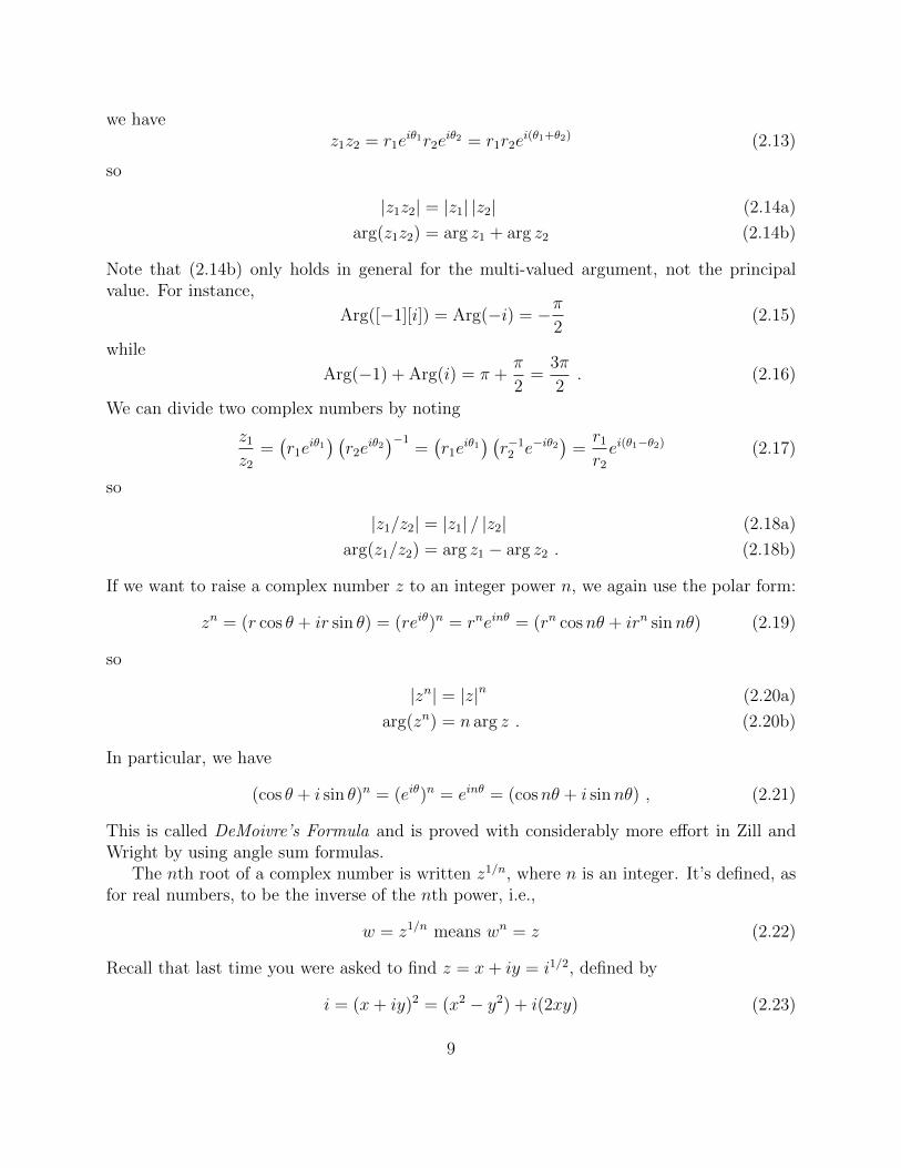
we havez1z2 = r1e

iθ1r2eiθ2 = r1r2e

i(θ1+θ2) (2.13)

so

|z1z2| = |z1| |z2| (2.14a)

arg(z1z2) = arg z1 + arg z2 (2.14b)

Note that (2.14b) only holds in general for the multi-valued argument, not the principalvalue. For instance,

Arg([−1][i]) = Arg(−i) = −π2

(2.15)

while

Arg(−1) + Arg(i) = π +π

2=

3π

2. (2.16)

We can divide two complex numbers by noting

z1

z2

=(r1e

iθ1) (r2e

iθ2)−1

=(r1e

iθ1) (r−1

2 e−iθ2)

=r1

r2

ei(θ1−θ2) (2.17)

so

|z1/z2| = |z1| / |z2| (2.18a)

arg(z1/z2) = arg z1 − arg z2 . (2.18b)

If we want to raise a complex number z to an integer power n, we again use the polar form:

zn = (r cos θ + ir sin θ) = (reiθ)n = rneinθ = (rn cosnθ + irn sinnθ) (2.19)

so

|zn| = |z|n (2.20a)

arg(zn) = n arg z . (2.20b)

In particular, we have

(cos θ + i sin θ)n = (eiθ)n = einθ = (cosnθ + i sinnθ) , (2.21)

This is called DeMoivre’s Formula and is proved with considerably more effort in Zill andWright by using angle sum formulas.

The nth root of a complex number is written z1/n, where n is an integer. It’s defined, asfor real numbers, to be the inverse of the nth power, i.e.,

w = z1/n means wn = z (2.22)

Recall that last time you were asked to find z = x+ iy = i1/2, defined by

i = (x+ iy)2 = (x2 − y2) + i(2xy) (2.23)

9

This is equivalent to the system of two real equations

x2 − y2 = 0 (2.24a)

2xy = 1 (2.24b)

which has two solutions for (x, y): (√

2/2,√

2/2) or (−√

2/2,−√

2/2). This means

i1/2 =

√2

2+ i

√2

2or −

√2

2− i√

2

2(2.25)

In practice, it’s much easier to take roots of a complex number using the polar form, i.e.,writing

z = reiθ = wn = ρeinφ (2.26)

as equivalent tow = ρeiφ = z1/n = (reiθ)1/n (2.27)

It’s tempting to just identify ρ with n√r and φ with θ/n, but there’s a catch. Because of the

periodicity of the angle θ, the complex number z is unchanged if we add any multiple of 2πto θ. So

z = ei(θ+k 2π) (2.28)

where k is any integer. Butθ + k 2π

n=θ

n+k

n2π (2.29)

gives physically different angles if k/n is not an integer. This means that in general, if z 6= 0,there are n distinct roots z1/n, given by∣∣z1/n

∣∣ = n√|z| (2.30a)

arg(z1/n) =

{arg z

n+k

n2π

∣∣∣∣ k = 0, 1, . . . , n− 1

}(2.30b)

for k = 0, 1, . . . , n.Example: what is (−8i)1/3? First we take the modulus and argument of −8i. Its modulus

is 8 and its argument is −π/2. The three cube roots all have modulus 3√

8 = 2 and theirarguments are

1

3

(−π

2

)= −π

6(2.31a)

1

3

(−π

2+ 2π

)= −π

6+

2π

3=

(4− 1)π

6=π

2(2.31b)

1

3

(−π

2+ 4π

)= −π

6+

4π

3=

(8− 1)π

6=

7π

6= 2π − 5π

6(2.31c)

10

which makes the three cube roots (referring to the table at the beginning of today’s notes)

2e−iπ/6 = 2[cos(−π

6

)+ i sin

(−π

6

)]= 2

[√3

2− i1

2

]=√

3− i (2.32a)

2eiπ/2 = 2[cos

π

2+ i sin

π

2

]= 2 [0 + i] = 2i (2.32b)

2ei7π/6 = 2e−i5π/6 = 2

[cos

(−5π

6

)+ i sin

(−5π

6

)]= 2

[−√

3

2− i1

2

]= −√

3− i (2.32c)

If we look on the complex plane, we see that the roots are evenly spaced along a circle ofradius 2:

11

2.3 Regions in the Complex Plane

Recall that we can’t talk about one complex number being greater than or less than another.But we can apply these inequalities to real quantities constructed from complex numbers,like |z|, arg z, Re(z) and Im(z). This will be very useful, since it will allow us to talk aboutone complex number being “close to” another. If we think of complex numbers as pointsin the complex plane, the natural distance between two complex numbers z1 = x1 + iy1

and z2 = x2 + iy2 is the distance between the points (x1, y1) and (x2, y2) arising from thePythagorean theorem:

√(x2 − x1)2 + (y2 − y1)2 = |(x2 − x1) + i(y2 − y1)| = |z2 − z1| (2.33)

If we take a fixed point z0 in the complex plane, and a constant positive number ρ, thenthe equation

|z − z0| = ρ (2.34)

defines the set of all points z which are a distance ρ away from z0. This is a circle of radiusρ centered on z0, as we can easily see by writing z = x+ iy and z0 = x0 + iy0 and squaringboth sides of (2.34):

(x− x0)2 + (y − y0)2 = ρ2 (2.35)

12

If we replace the equation (2.34) with an inequality, we get a set of complex numbers,corresponding to a region in the complex plane. For example, |z − z0| ≤ ρ is the interior ofthe circle of radius ρ centered at z0, including its boundary. A set like this, which includes itsboundary, is called a closed set. If we do not include the boundary |z − z0| = ρ, we insteadget what’s called an open set |z − z0| < ρ which is the interior of the circle, not including itsboundary:

We can create closed and open sets using a variety of inequalities. Each one is constructedfrom some real function(s) of the complex number z. See Zill and Wright for more examples.

13

Practice Problems

17.2.7, 17.2.11, 17.2.13, 17.2.23, 17.2.33, 17.2.39, 17.3.5, 17.3.17

Tuesday 13 September 2011

3 Functions of a Complex Variable

3.1 Complex Functions

Recall the definition of a function in real analysis. A function f is a “machine” which takesa number x and spits out another number f(x). So for example, if f(x) = x2 + 1, thenf(2) = 5. We talk about a function having a domain (the set of all numbers you can putinto it) and a range (the set of all numbers that can come out of it). So for example iff(x) =

√x then the domain and range of f are both [0,∞).

In complex analysis, a function is a “machine” which takes a complex number z and spitsout another complex number w = f(z). So if f(z) = z2 + 1 then f(2) = 5, f(i) = 0, andf(1 + i) = 1 + 2i. Because output w = u + iv of f has a real part and an imaginary partwhich both depend on the real and imaginary part of the input z = x+ iy, we can also thinkof f as a machine which takes in two real numbers and spits out two real numbers:

f(z) = f(x+ iy) = u(x, y) + iv(x, y) (3.1)

For any complex function f(z) there is a corresponding pair of real functions of two realvariables, u(x, y) and v(x, y). For example, if f(z) = z2 + 1,

u(x, y) + iv(x, y) = f(z) = (x+ iy)2 + 1 = x2 + 2ixy− y2 + 1 = (x2− y2 + 1) + i(2xy) (3.2)

which means that

u(x, y) = x2 − y2 + 1 (3.3a)

v(x, y) = 2xy (3.3b)

Similarly, given any two real functions u(x, y) and v(x, y), I can construct a complex functionf(z) = f(x+ iy) = u(x, y) + iv(x, y), although the result might not be writable as a simpleexpression involving z.

3.1.1 Visualizing Complex Functions

With a real function f(x) we can just draw a two-dimensional graph with x on one axis andf(x) on the other. With a complex function of a complex argument, this is not so easy,since we’d need to draw a surface in a four-dimensional space to show the u and v valuescorresponding to each x and y. Instead, we start with the complex plane, which is a two-dimensional space with coordinates x and y. Each point is a complex number z = x+iy, andwe can then imagine the function f defining a complex number f(z) = w = u(x, y)+ iv(x, y)at each point. There are a few possibilities:

14

Use color: If we write the function in polar form

f(z) = ρ(x, y)eiφ(x,y) (3.4)

then we can represent the value f(z) by a color, where the modulus ρ determines how brightthe color is and the argument φ determines the hue (red, green, cyan, yellow, etc., whichis handy because hue is periodic around the color wheel just like the angular coordinate isperiodic). So 0 would be black, real numbers would be either shades of red that got brighterand brighter as they got more positive or shades of cyan that got brighter and brighter asthey got more negative, and in general complex numbers would get brighter and brighter asyou went off away from zero in any direction. Here’s an example of one such scheme:

There are lots of fine points, like whether it’s really a good idea to use red for positivenumbers Arg(z) = 0, and the fact that we perceive some hues as being inherently brighterthan others,4 but you’ll see these sorts of visualizations around the web.

Use vectors: Just as we can use the coordinates (x, y) to associate a number z = x + iywith a point in the plane, we can think of u and v as the components of a vector in twodimensions, and if we recall that u(x, y) and v(x, y) gives us two numbers at each point, wecan use the function f(z) to construct a vector field, i.e., a prescription for defining a vectorat each point. The most obvious choice is to use u as the x component and v as the realcomponent, i.e., to define the vector field5

~T (x, y) = u(x, y) x+ v(x, y) y (3.5)

4Ask your friends majoring in Color Science!5You may have seen the unit vectors in the x and y directions written as ı and ; Zill and Wright refer to

them as i and j. To avoid confusion between the vector i and the complex number i, I’ll call them x and y.

15

This is the vector field that Zill and Wright uses throughout the book.It turns out, though, that there’s a different choice which makes some of the connections

between complex analysis and vector calculus more straightforward. That is called the Polyavector field

~H(x, y) = u(x, y) x− v(x, y) y (3.6)

Here are some examples of both vector fields:

Map the z plane into the w plane: Finally, rather than trying to represent the complexnumber w = f(z) at each point in the complex plane, we can imagine two planes, side

16

by side, one representing z and the other representing w, and consider the function f asmapping the first plane onto the second plane. For instance, if f(z) = z2 + 1, consider theline x = 1, which runs parallel to the imaginary axis. Each possible value of y correspondsto a point on this line. Using

u(x, y) = x2 − y2 + 1 (3.3a)

v(x, y) = 2xy (3.3b)

we note that the corresponding curve in the w plane is

u(1, y) = 2− y2 (3.7a)

v(1, y) = 2y (3.7b)

The curve, written in terms of u and v, is u = 2− v2/4, which describes a parabola.On the other hand, the line y = 1 is parallel to the real axis, and its image is parameterized

as

u(x, 1) = x2 (3.8a)

v(x, 1) = 2x (3.8b)

which is the parabola u = v2/4We can plot these curves, the first in red and the second in blue:

17

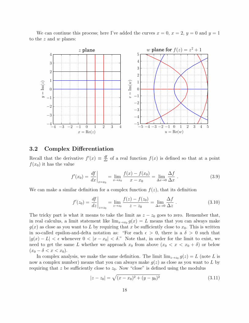
We can continue this process; here I’ve added the curves x = 0, x = 2, y = 0 and y = 1to the z and w planes:

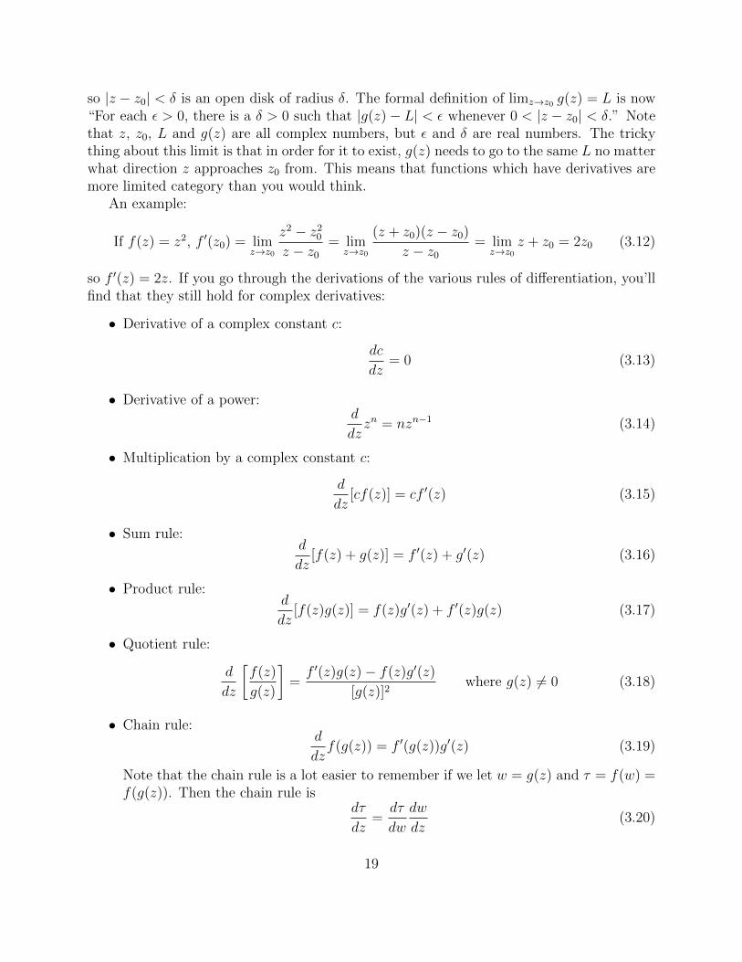
3.2 Complex Differentiation

Recall that the derivative f ′(x) ≡ dfdx

of a real function f(x) is defined so that at a pointf(x0) it has the value

f ′(x0) =df

dx

∣∣∣∣x=x0

= limx→x0

f(x)− f(x0)

x− x0

= lim∆x→0

∆f

∆x. (3.9)

We can make a similar definition for a complex function f(z), that its definition

f ′(z0) =df

dz

∣∣∣∣z=z0

= limz→z0

f(z)− f(z0)

z − z0

= lim∆z→0

∆f

∆z. (3.10)

The tricky part is what it means to take the limit as z − z0 goes to zero. Remember that,in real calculus, a limit statement like limx→x0 g(x) = L means that you can always makeg(x) as close as you want to L by requiring that x be sufficiently close to x0. This is writtenin so-called epsilon-and-delta notation as: “For each ε > 0, there is a δ > 0 such that|g(x)− L| < ε whenever 0 < |x− x0| < δ.” Note that, in order for the limit to exist, weneed to get the same L whether we approach x0 from above (x0 < x < x0 + δ) or below(x0 − δ < x < x0).

In complex analysis, we make the same definition. The limit limz→z0 g(z) = L (note L isnow a complex number) means that you can always make g(z) as close as you want to L byrequiring that z be sufficiently close to z0. Now “close” is defined using the modulus

|z − z0| =√

(x− x0)2 + (y − y0)2 (3.11)

18

so |z − z0| < δ is an open disk of radius δ. The formal definition of limz→z0 g(z) = L is now“For each ε > 0, there is a δ > 0 such that |g(z)− L| < ε whenever 0 < |z − z0| < δ.” Notethat z, z0, L and g(z) are all complex numbers, but ε and δ are real numbers. The trickything about this limit is that in order for it to exist, g(z) needs to go to the same L no matterwhat direction z approaches z0 from. This means that functions which have derivatives aremore limited category than you would think.

An example:

If f(z) = z2, f ′(z0) = limz→z0

z2 − z20

z − z0

= limz→z0

(z + z0)(z − z0)

z − z0

= limz→z0

z + z0 = 2z0 (3.12)

so f ′(z) = 2z. If you go through the derivations of the various rules of differentiation, you’llfind that they still hold for complex derivatives:

• Derivative of a complex constant c:

dc

dz= 0 (3.13)

• Derivative of a power:d

dzzn = nzn−1 (3.14)

• Multiplication by a complex constant c:

d

dz[cf(z)] = cf ′(z) (3.15)

• Sum rule:d

dz[f(z) + g(z)] = f ′(z) + g′(z) (3.16)

• Product rule:d

dz[f(z)g(z)] = f(z)g′(z) + f ′(z)g(z) (3.17)

• Quotient rule:

d

dz

[f(z)

g(z)

]=f ′(z)g(z)− f(z)g′(z)

[g(z)]2where g(z) 6= 0 (3.18)

• Chain rule:d

dzf(g(z)) = f ′(g(z))g′(z) (3.19)

Note that the chain rule is a lot easier to remember if we let w = g(z) and τ = f(w) =f(g(z)). Then the chain rule is

dτ

dz=dτ

dw

dw

dz(3.20)

19

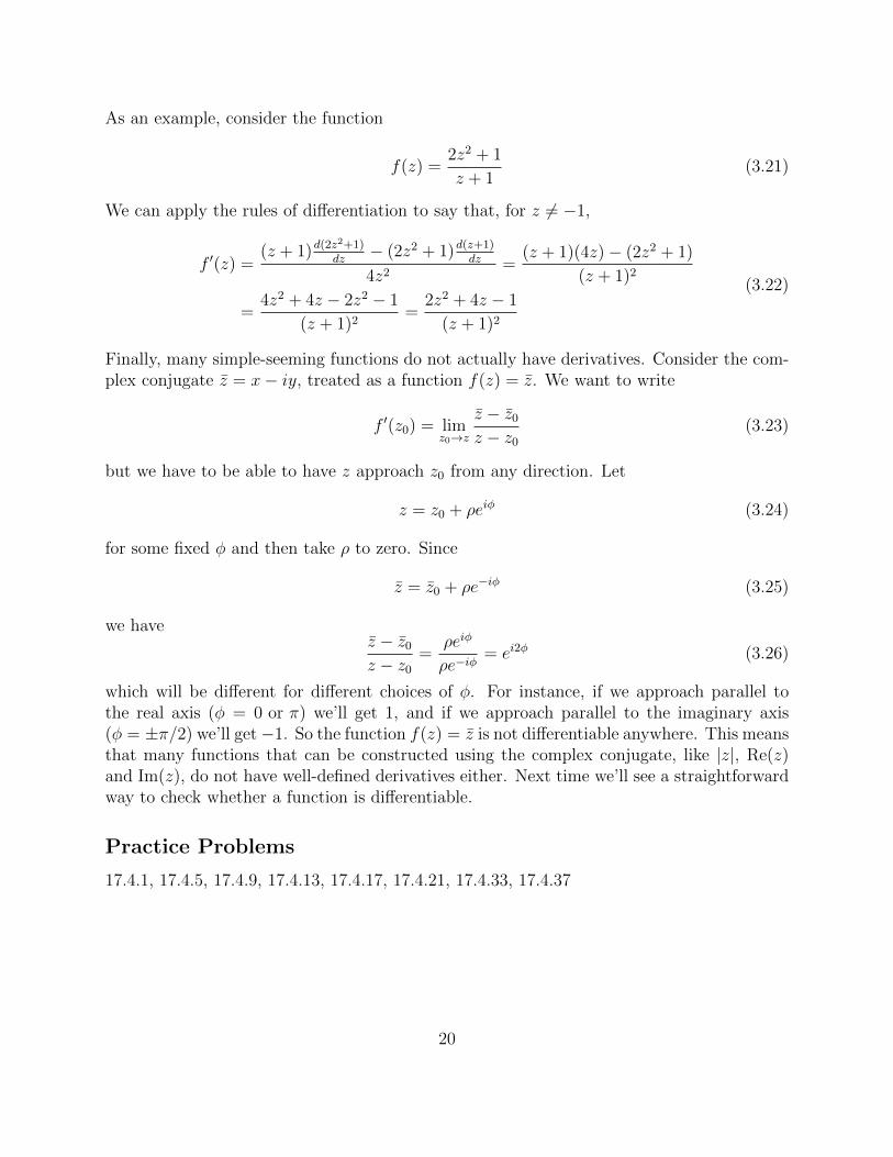
As an example, consider the function

f(z) =2z2 + 1

z + 1(3.21)

We can apply the rules of differentiation to say that, for z 6= −1,

f ′(z) =(z + 1)d(2z2+1)

dz− (2z2 + 1)d(z+1)

dz

4z2=

(z + 1)(4z)− (2z2 + 1)

(z + 1)2

=4z2 + 4z − 2z2 − 1

(z + 1)2=

2z2 + 4z − 1

(z + 1)2

(3.22)

Finally, many simple-seeming functions do not actually have derivatives. Consider the com-plex conjugate z = x− iy, treated as a function f(z) = z. We want to write

f ′(z0) = limz0→z

z − z0

z − z0

(3.23)

but we have to be able to have z approach z0 from any direction. Let

z = z0 + ρeiφ (3.24)

for some fixed φ and then take ρ to zero. Since

z = z0 + ρe−iφ (3.25)

we havez − z0

z − z0

=ρeiφ

ρe−iφ= ei2φ (3.26)

which will be different for different choices of φ. For instance, if we approach parallel tothe real axis (φ = 0 or π) we’ll get 1, and if we approach parallel to the imaginary axis(φ = ±π/2) we’ll get−1. So the function f(z) = z is not differentiable anywhere. This meansthat many functions that can be constructed using the complex conjugate, like |z|, Re(z)and Im(z), do not have well-defined derivatives either. Next time we’ll see a straightforwardway to check whether a function is differentiable.

Practice Problems

17.4.1, 17.4.5, 17.4.9, 17.4.13, 17.4.17, 17.4.21, 17.4.33, 17.4.37

20

Thursday 15 September 2011

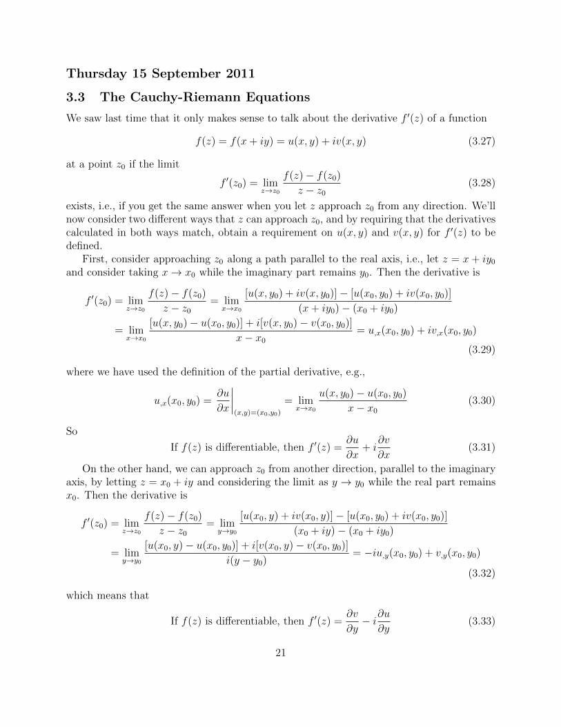
3.3 The Cauchy-Riemann Equations

We saw last time that it only makes sense to talk about the derivative f ′(z) of a function

f(z) = f(x+ iy) = u(x, y) + iv(x, y) (3.27)

at a point z0 if the limit

f ′(z0) = limz→z0

f(z)− f(z0)

z − z0

(3.28)

exists, i.e., if you get the same answer when you let z approach z0 from any direction. We’llnow consider two different ways that z can approach z0, and by requiring that the derivativescalculated in both ways match, obtain a requirement on u(x, y) and v(x, y) for f ′(z) to bedefined.

First, consider approaching z0 along a path parallel to the real axis, i.e., let z = x + iy0

and consider taking x→ x0 while the imaginary part remains y0. Then the derivative is

f ′(z0) = limz→z0

f(z)− f(z0)

z − z0

= limx→x0

[u(x, y0) + iv(x, y0)]− [u(x0, y0) + iv(x0, y0)]

(x+ iy0)− (x0 + iy0)

= limx→x0

[u(x, y0)− u(x0, y0)] + i[v(x, y0)− v(x0, y0)]

x− x0

= u,x(x0, y0) + iv,x(x0, y0)

(3.29)

where we have used the definition of the partial derivative, e.g.,

u,x(x0, y0) =∂u

∂x

∣∣∣∣(x,y)=(x0,y0)

= limx→x0

u(x, y0)− u(x0, y0)

x− x0

(3.30)

So

If f(z) is differentiable, then f ′(z) =∂u

∂x+ i

∂v

∂x(3.31)

On the other hand, we can approach z0 from another direction, parallel to the imaginaryaxis, by letting z = x0 + iy and considering the limit as y → y0 while the real part remainsx0. Then the derivative is

f ′(z0) = limz→z0

f(z)− f(z0)

z − z0

= limy→y0

[u(x0, y) + iv(x0, y)]− [u(x0, y0) + iv(x0, y0)]

(x0 + iy)− (x0 + iy0)

= limy→y0

[u(x0, y)− u(x0, y0)] + i[v(x0, y)− v(x0, y0)]

i(y − y0)= −iu,y(x0, y0) + v,y(x0, y0)

(3.32)

which means that

If f(z) is differentiable, then f ′(z) =∂v

∂y− i∂u

∂y(3.33)

21

In order for the derivative to be well-defined, (3.31) and (3.33) have to agree, i.e.,

If f(z) is differentiable, then∂u

∂x+ i

∂v

∂x=∂v

∂y− i∂u

∂y(3.34)

Splitting this equation into its real and imaginary parts gives us the Cauchy-Riemann equa-tions

∂u

∂x=∂v

∂y(3.35a)

∂v

∂x= −∂u

∂y(3.35b)

These equations have to be satisfied at any point where f(z) is differentiable. This meansthey are a necessary condition for differentiability. We won’t show it right now, but it turnsout that they are also sufficient, i.e., if the Cauchy-Riemann equations are satisfied, and all ofthe partial derivatives are continuous, the function is differentiable. (This is basically becauseif you know how to approach along the real direction and along the imaginary direction, youcan describe the results of approaching along an arbitrary direction as a superposition of thetwo.)

3.3.1 The Fine Print: Differentiable vs Analytic

If the complex derivative f ′(z0) exists, we say f(z) is differentiable at z0. A closely relatedterm is analytic; we say that f(z) is analytic at z0 if it is differentiable in some open region(“domain”) containing z0. (That was the point of all of that neighborhood business insection 17.3.) The bottom line is that if the Cauchy-Riemann equations are satisfied in anopen region, and all of the partial derivatives are continuous, the function is analytic in thatregion.

As an example of the difference between differentiable and analytic, consider the function

f(z) = [Re(z)]2 = x2 (3.36)

which has u(x, y) = x2 and v(x, y) = 0. The partial derivatives are

∂u

∂x= 2x

∂v

∂x= 0 (3.37a)

∂u

∂y= 0

∂v

∂y= 0 (3.37b)

And we see that the Cauchy-Riemann equations are satisfied if x = 0 but not otherwise.The line x = 0 is the imaginary axis, and it’s just a line. So f(z) is differentiable along thatline, but since any neighborhood contains some points not on that line, it is not analyticanywhere.

22

3.3.2 Aside: Vector Calculus

If we write the Cauchy-Riemann equations (3.35) as

∂u

∂x− ∂v

∂y= 0 (3.38a)

∂v

∂x+∂u

∂y= 0 (3.38b)

they should look kind of reminiscent of derivatives from vector calculus.In two dimensions there are two interesting derivatives you can take of a vector field

~F (x, y) = Fx(x, y) x+ Fy(x, y) y . (3.39)

(Note that Fx and Fy are components of ~F , not partial derivatives.) The two derivatives arethe divergence and the curl:

div ~F =∂Fx∂x

+∂Fy∂y

(3.40a)

curl ~F =∂Fy∂x− ∂Fx

∂y(3.40b)

In three dimensions the divergence div ~F is the scalar field div ~F = ~∇ · ~F , and the curlcurl ~F is the vector field ~∇× ~F , but in two dimensions, you can just think of each of them asproducing a scalar field, i.e., a number for each point in the plane. We can see the geometricalmeaning if we sketch vector fields with locally positive divergence or curl:

23

The vector field on the left, which has Fx increasing with x and Fy increasing with y, is“diverging” out from the point in the middle; if we calculated the outward flux of the vectorfield through a small bubble around that point, it would be positive.

The vector field on the right, which has Fy increasing with x and Fx decreasing with y,is “curling” counter-clockwise around the point in the middle; if we calculated the counter-clockwise circulation of the vector field around a small curve encircling that point, it wouldbe positive.

Now consider the Polya vector field

~H = u(x, y) x− v(x, y)y (3.41)

which we defined last time. Its divergence and curl are

div ~H =∂u

∂x+∂(−v)

∂y=∂u

∂x− ∂v

∂y(3.42a)

curl ~H =∂u

∂y− ∂(−v)

∂x=∂u

∂y+∂v

∂x(3.42b)

but these are exactly the expressions in (3.38), which vanish when the Cauchy-Riemannequations are satisfied. This means that the Cauchy-Riemann equations for a functionare equivalent to that function’s Polya vector field having zero divergence andzero curl.6

3.3.3 Harmonic Functions

The Cauchy-Riemann equations are a pair of conditions on the two functions u(x, y) andv(x, y) together, but they also imply a separate differential equation for u(x, y), and anotherone for v(x, y). If we take the partial derivative of the first equation with respect to x andof the second equation with respect to y, we get

∂

∂x

∂u

∂x=

∂

∂x

∂v

∂y(3.43a)

∂

∂y

∂v

∂x= − ∂

∂y

∂u

∂y(3.43b)

Now, it is a property of partial derivatives that, if the functions involved have continuouspartial derivatives, the partial derivatives commute. In this case,

∂

∂x

∂v

∂y=

∂2v

∂x∂y=

∂2v

∂y∂x=

∂

∂y

∂v

∂x(3.44)

6This is one of the reasons the Polya vector field ~H = u(x, y) x − v(x, y)y is more convenient than the

field ~T = u(x, y) x+ v(x, y)y which Zill and Wright use. The divergence and curl of ~T vanish if and only ifthe complex conjugate function f(z) = u(x, y)− iv(x, y) satisfies the Cauchy-Riemann equations.

24

This means that the two expressions in (3.43) are equal to each other, and

∂2u

∂x2= −∂

2u

∂y2(3.45)

I.e., u(x, y) solves Laplace’s equation

∂2u

∂x2+∂2u

∂y2= 0 (3.46)

We say that u(x, y) is a harmonic function. We can go through the same argument with thederivatives switched, and from

∂

∂y

∂u

∂x=

∂

∂y

∂v

∂y(3.47a)

∂

∂x

∂v

∂x= − ∂

∂x

∂u

∂y(3.47b)

deduce∂2v

∂x2+∂2v

∂y2= 0 (3.48)

That means that if f(z) = u(x, y) + iv(x, y) is an analytic function, the functionsu(x, y) and v(x, y) are both harmonic. We refer to v(x, y) as the conjugate harmonicfunction of u(x, y) and vice versa.

If we start with a harmonic function u(x, y), we can deduce its conjugate harmonicfunction v(x, y), up to a constant, by imposing the Cauchy-Riemann equations

∂v

∂x= −∂u

∂y(3.49a)

∂v

∂y=∂u

∂x(3.49b)

Example: Let u(x, y) = x2 − y2 + 2x. We can check that it is harmonic by calculating

∂u

∂x= 2x+ 2

∂2u

∂x2= 2 (3.50a)

∂u

∂y= −2y

∂2u

∂y2= −2 (3.50b)

(3.50c)

so we do indeed have ∂2u∂x2

+ ∂2u∂y2

= 0. We can find y from the differential equations

∂v

∂x= −∂u

∂y= 2y (3.51a)

∂v

∂y=∂u

∂x= 2x+ 2 (3.51b)

25

Integrating (3.51a) with respect to x gives

v(x, y) =

∫2y dx = 2xy + h(y) ; (3.52)

The integration “constant” is actually an arbitrary function of y alone, because such afunction acts like a constant when we take the partial derivative with respect to x. Plugging(3.52) into (3.51b) gives us

∂v

∂y= 2x+ h′(y) = 2x+ 2 (3.53)

which means thath′(y) = 2 (3.54)

this meansh(y) = 2y + C (3.55)

where now C really is a constant, so the conjugate harmonic function of u(x, y) = x2−y2+2xis

v(x, y) = 2xy + 2y + C (3.56)

The function isf(z) = x2 − y2 + 2x+ i(2xy + 2y + C) (3.57)

The conjugate harmonic function is not just a handy way of taking one harmonic functionand generating another; the functions u(x, y) and v(x, y) also have level surfaces (u(x, y) =const and v(x, y) = const which meet at right angles).

Practice Problems

17.5.1, 17.5.3, 17.5.9, 17.5.15, 17.5.17, 17.5.23, 17.5.25, 17.5.29, 17.5.32

Tuesday 20 September 2011

3.4 Some Specific Functions

The various rules of differentiation (sum, product, quotient, etc) mean that we can build upanalytic functions from polynomials; for example, if n is a positive integer, zn is analyticeverywhere (with derivative nzn−1) and z−n is analytic (with derivative−nz−(n+1) everywhereexcept at z = 0. We now consider the behavior of some transcendental functions on thecomplex plane.

26

3.4.1 Exponentials, Logarithms and Powers

We already know how to take the exponential ex of a real number x, and Euler’s formulalets us take the exponential eiy = cos y + i sin y of an imaginary number iy. So for a generalcomplex number z = x+ iy, the exponential function is

ez = ex+iy = exeiy = ex cos y + iex sin y (3.58)

We can check that it’s analytic by verifying that

u(x, y) = ex cos y (3.59a)

v(x, y) = ex sin y (3.59b)

satisfy the Cauchy-Riemann equations. The partial derivatives are

∂u

∂x= ex cos y

∂v

∂x= ex sin y (3.60a)

∂u

∂y= −ex sin y

∂v

∂y= ex cos y (3.60b)

from which we can see that indeed ∂v∂y

= ∂u∂x

and ∂v∂x

= −∂u∂y

.Note that the exponential function is periodic in the complex direction:

ez+i2nπ = ez n ∈ Z (3.61)

This can be seen in a color plot of the exponential function:

27

The natural logarithm is the inverse of the exponential function. This is complicated bythe fact that the function ez is not one-to-one, i.e., there are many values of w such thatz = ew. For example, i = eiπ/2 = ei3π/2 = e−iπ/2 etc. This is the same issue we have withroots like z1/5. To talk about the specific value of the logarithm, we need to spell out somenotation; here are the names given by Zill and Wright for the different natural logarithms:

• loge is the natural logarithm as a real number; it is a one-to-one and onto functionwhich takes positive real numbers (0,∞) to real numbers (−∞,∞). It is the inverseof the exponential, so eloge(x) = x and loge(e

x) = x.

• ln z is a multi-valued complex “function”, defined so that w = ln z if w is any numbersuch that z = ew.

• Ln z is the principal value of the natural logarithm, which is the inverse of the expo-nential, with w = Ln z restricted to lie in the region −π < Lnw < π

To work out the possible values of the multi-valued natural logarithm w = u + iv = ln z =ln(x+ iy) = ln(reiθ) we require that ew = z, i.e.,

reiθ = x+ iy = z = ew = eu+iv = eueiv = eu cos v + ieu sin v (3.62)

For this to be satisfied, we need

x = eu cos v (3.63a)

y = eu sin v (3.63b)

28

or equivalently

r = eu (3.64a)

eiθ = eiv (3.64b)

The first equation relates two positive real numbers, so we can take the natural logarithmand find

u = loge r = loge√x2 + y2 ; (3.65)

The second equation says that v can be any number such that

cos v = cos θ =x

r(3.66a)

sin v = sin θ =y

r(3.66b)

which means v can be θ plus any integer multiple of 2π. But that’s just the multi-valuedargument of z

arg z = atan2(y, x) + n2π n ∈ Z (3.67)

This means the multi-valued natural logarithm is

ln z = loge |z|+ i arg z (3.68)

The principal value just comes from taking the principal value of the argument:

Ln z = loge |z|+ iArg z (3.69)

The usual nice features of the logarithm apply to the multi-valued complex logarithm,e.g.,

ln(z1z2) = ln z1 + ln z1 (3.70a)

lnz1

z2

= ln z1 − ln z1 (3.70b)

Again, this may not hold for the principal values, e.g., let z1 = −1 + i and z2 = i. Then|z1| =

√2, Arg(z1) = atan2(1,−1) = 3π/4, |z2| = 1, Arg(z2) = atan2(1, 0) = π/2. So

Ln z1 = Ln(1 + i) = loge(√

2) + i3π

4=

1

2loge 2 + i

3π

4(3.71a)

Ln z2 = Ln(i) = loge(1) + iπ

2= i

π

2(3.71b)

On the other hand, z1z2 = (−1+i)(i) = −1−i, so |z1z2| =√

2, and Arg(z1z2) atan2(−1,−1) =−3π/4. This means that

Ln(z1z2) = Ln(−1− i) = loge(√

2)− i3π4

=1

2loge 2− i3π

4(3.72)

29

On the other hand,

Ln z1 + Ln z2 = loge(√

2) + i3π

4+ iπ =

1

2loge 2 + i

5π

4(3.73)

so we see they differ by a multiple of 2π.If consider Ln z as a complex function

Ln z = Ln(x+ iy) = loge |z|+ iArg z =1

2loge(x

2 + y2) + i atan2(y, x) (3.74)

then f(z) = Ln z = u(x, y) + iv(x, y) has real and imaginary parts

u(x, y) =1

2loge(x

2 + y2) (3.75a)

v(x, y) = atan2(y, x) = Arg(x+ iy) (3.75b)

We see that both u(x, y) and v(x, y) are undefined at the origin (x, y) = (0, 0). They’redefined everywhere else, but v(x, y) is discontinuous on the negative x axis, since atan2(y, x)is defined to be π if x < 0 and y = 0, but it approaches −π as we approach the negative xaxis from the fourth quadrant. So Ln z is undefined at z = 0 and it’s discontinuous on thenegative real axis, but it’s continuous everywhere else. You can also show that it’s analyticon that region7, but we’ll just show what the derivative must be, by implicit differentiation:If w = Ln z, so that z = ew, then, by the chain rule,

1 = ewdw

dz= z

dw

dz(3.76)

but dividing by z gives

dw

dz=

d

dzLn z =

1

zunless z is non-positive real number (3.77)

Note that as we move around the complex plane, the multi-valued ln z, like the multi-valued arg(z), is continuous everywhere except for the origin z = 0, but if we go oncecounter-clockwise around the origin, arg z has increased by 2π, and ln z has increased byi2π, from where we started. We can visualize a “parking ramp” where going around theorigin moves us smoothly up to another level:

7You have to consider the derivatives of atan2(y, x), which are basically the derivatives of the polarcoordinate θ with respect to x and y.

30

Choosing a single principal value for Ln z or Arg z means picking one “branch” of this surface,and imposing a discontinuity called a “branch cut”. Our choice is to put the branch cut alongthe negative real axis, but we could have made a different choice, like requiring 0 ≤ θ < 2π.

Complex powers: Finally, note that the complex logarithm lets us talk about raising acomplex number to an arbitrary complex power. Recall that if x is a positive real numberand a is any real number, taking the exponential of both sides of

loge(xa) = a loge x (3.78)

allows us to writexa = ea loge x ; (3.79)

for complex numbers z and α, we define

zα = eα ln z (3.80)

In general, since

ln z = loge |z|+ i arg z = loge |z|+ iArg z + i k2π k ∈ Z (3.81)

there are an infinite number of values for zα:

zα = exp [α loge |z|+ i α(Arg z + k2π)] (3.82)

31

Note that in the special case where α = n, a real integer, we get

zn = exp [n loge |z|+ i n(Arg z + k2π)] = |z|n e−i nArg zei nk2π = |z|n e−i nArg z (3.83)

which is a single value, because ei nk2π = 1. When α = m/n, a rational number with m andn being integers with no non-trivial common factor, we get a similar case to what we hadwith roots:

zm/n = exp[mn

loge |z|+ im

n(Arg z + k2π)

]=√n |z|m eimArg(z)/nei 2πmk/n (3.84)

the last factor, ei 2πmk/n takes on different values for k = 0, 1, . . . (n−1), but it starts repeatingitself for k ≥ n or k < 0, which means there are n unique values for zm/n. This is also truefor real numbers.

Example: what are the different values of 641/6? Well, since 64 = 26, and Arg(64) = 0,we get

11/6 = 2ei 2πk/6 = 2ei kπ/3 k = 0, 1, 2, 3, 4, 5 (3.85)

working out the trig functions gives the six roots

2ei0 = 2 (3.86a)

2eiπ/3 = 2 cosπ

3+ i2 sin

π

3= 1 + i

√3 (3.86b)

2ei2π/3 = 2 cos2π

3+ i2 sin

2π

3= −1 + i

√3 (3.86c)

2eiπ = −2 (3.86d)

2ei4π/3 = 2 cos4π

3+ i2 sin

4π

3= −1− i

√3 (3.86e)

2ei5π/3 = 2 cos5π

3+ i2 sin

5π

3= 1− i

√3 (3.86f)

Practice Problems

17.6.3, 17.6.7, 17.6.15, 17.6.23, 17.6.25, 17.6.33, 17.6.35, 17.6.41

32

Thursday 22 September 2011

3.4.2 Trigonometric and Hyperbolic Functions

If we recall the Euler relationeiθ = cos θ + i sin θ (3.87)

and alsoe−iθ = cos(−θ) + i sin(−θ) = cos θ − i sin θ (3.88)

we see that the sine and cosine of a real number θ can be written

cos θ =eiθ + e−iθ

2(3.89a)

sin θ =eiθ − e−iθ

2i(3.89b)

From which we have

tan θ =eiθ + e−iθ

eiθ − e−iθ(3.90)

and similar expressions for sec θ, csc θ, and cot θ. These relations are also the inspiration forthe definition of the hyperbolic trig functions

cosh η =eη + e−η

2(3.91a)

sinh η =eη − e−η

2(3.91b)

with analogous definitions for tanh η, sech η, etc.These definitions can be extended to complex arguments, i.e.,

cos z =eiz + e−iz

2(3.92a)

sin z =eiz − e−iz

2i(3.92b)

cosh z =ez + e−z

2(3.92c)

sinh z =ez − e−z

2(3.92d)

Since eαz is analytic over the whole complex plane (we say eαz is entire), the same is true forcos z, sin z, cosh z and cosh z. When we define other trigonometric and hyperbolic functionslike sec z = 1

cos zand tanh z = sinh z

cosh z, they’ll be analytic except where their denominators go

to zero. So it’s useful to sort out the zeros of sin z and cos z.We know that the real values at which sin z = 0 are integer multiples of π, and the real

values at which cos z = 0 are odd half-integer multiples of π, but are there any that are not

33

on the real axis? If we write sin z and cos z in the form f(z) = u(x, y) + iv(x, y) we get

cos z = cos(x+ iy) =1

2

(eixe−y + e−ixey

)=

1

2

(cosx e−y + i sinx e−y + cosx ey − i sinx ey

)= cosx cosh y − i sinx sinh y

(3.93)

A similar calculation shows

sin z = sinx cosh y + i cosx sinh y (3.94)

Now, to get sin z = 0, we have to have sin x cosh y = 0 and cosx sinh y = 0. Since cosh y ≥ 1for any real y, we need to have sinx = 0, which means x = nπ. In that case, cosx = (−1)n 6=0, which means we can only get cosx sinh y = 0 if sinh y = 0, i.e., y = 0. That means theonly zeros of sin z are the real ones:

sin z = 0 iff z ∈ {nπ|n ∈ Z} (3.95)

a similar argument shows that

cos z = 0 iff z ∈{(

n+1

2

)π

∣∣∣∣n ∈ Z}

(3.96)

To get the zeros of the hyperbolic sine and cosine, it helps to note that

cos(iz) =e−z + ez

2= cosh z (3.97)

and

sin(iz) =e−z − ez

2i= i sinh z (3.98)

This means that

cosh z = cos(−y + ix) = cosh x cos y + i sinhx sin y (3.99a)

sinh z = −i sin(−y + ix) = sinh x cos y + i coshx sin y (3.99b)

sosinh z = 0 iff z ∈ {i nπ|n ∈ Z} (3.100)

a similar argument shows that

cosh z = 0 iff z ∈{i

(n+

1

2

)π

∣∣∣∣n ∈ Z}

(3.101)

so the zeros of cosh z and sinh z are all along the imaginary axis.

34

The trigonometric functions are periodic in the real direction with period 2π, e.g., sin(z+2π) = sin(z):

Note that

sin(z +

π

2

)=eizeiπ/2 − e−ize−iπ/2

2i=ieiz − (−i)e−iz

2i=eiz + e−iz

2= cos z (3.102)

just as for real arguments. In fact the angle sum formulas still hold:

sin(z1 + z2) = sin z1 cos z2 + cos z1 sin z2 (3.103a)

cos(z1 + z2) = cos z1 cos z2 − sin z1 sin z2 (3.103b)

The hyperbolic functions are periodic in the imaginary direction, also with period 2π,e.g., cosh(z + 2π) = cosh(z):

35

Notice that since

sinh(z1 + z2) = sinh z1 cosh z2 + cosh z1 sinh z2 (3.104a)

cosh(z1 + z2) = cosh z1 cosh z2 + sinh z1 sinh z2 (3.104b)

we have

sinh(z + i

π

2

)= sinh z cosh

(iπ

2

)+cosh z sinh

(iπ

2

)= sinh z cos

π

2+ i cosh z sin

π

2= i cosh z

(3.105)

Practice Problems

17.7.5, 17.7.7, 17.7.11, 17.7.15, 17.7.19, 17.7.21, 17.7.29, 17.7.30

36

A Taylor Series and the Euler Relation

Math department graffiti: “eiπ = −1. Yeah, right.”But it is true. Unfortunately, have to prove with Taylor Series:

f(x) = f(0) + f ′(0)x+f ′′(0)

2x2 + . . . =

∞∑n=0

f (n)(0)

n!xn (A.1)

Apply this to three functions: eiθ, cos θ, and sin θ:f(θ) eiθ cos θ sin θf(0) 1 1 0f ′(θ) ieiθ − sin θ cos θf ′(0) i 0 1f ′′′(θ) −eiθ − cos θ − sin θf ′′′(0) −1 −1 0

f (4)(θ) −ieiθ sin θ − cos θ

f (4)(0) −i 0 −1

f (n)(0)(n even) (−1)n/2 = in (−1)n/2 = in 0

f (n)(0)(n odd) −1(n−1)/2i = in 0 −1(n−1)/2 = in−1

So the three Taylor series are

eiθ = 1 + iθ − 1

2θ2 − i

3!θ3 + . . . (A.2a)

cos θ = 1− 1

2θ2 + . . . (A.2b)

sin θ = θ − 1

3!θ3 + . . . (A.2c)

from which, along with

i sin θ = iθ − i

3!θ3 + . . . (A.3)

we seeeiθ = cos θ + i sin θ (A.4)

This is called the Euler relation.

37