Embed Size (px)
Citation preview
Ann Inst Stat Math (2009) 61:811–833DOI 10.1007/s10463-007-0161-1
Functional regression modeling via regularizedGaussian basis expansions
Yuko Araki · Sadanori Konishi ·Shuichi Kawano · Hidetoshi Matsui
Received: 22 September 2006 / Revised: 19 September 2007 / Published online: 31 January 2008© The Institute of Statistical Mathematics, Tokyo 2008
Abstract We consider the problem of constructing functional regression models forscalar responses and functional predictors, using Gaussian basis functions along withthe technique of regularization. An advantage of our regularized Gaussian basis expan-sions to functional data analysis is that it creates a much more flexible instrument fortransforming each individual’s observations into functional form. In constructing func-tional regression models there remains the problem of how to determine the numberof basis functions and an appropriate value of a regularization parameter. We presentmodel selection criteria for evaluating models estimated by the method of regulariza-tion in the context of functional regression models. The proposed functional regressionmodels are applied to Canadian temperature data. Monte Carlo simulations are con-ducted to examine the efficiency of our modeling strategies. The simulation resultsshow that the proposed procedure performs well especially in terms of flexibility andstable estimates.
Keywords Functional regression modeling · Gaussian basis function ·Regularization · Smoothing parameter selection
Y. Araki (B)Biostatistics Center, Kurume University, 67 Asahi-Machi, Kurume, Fukuoka 830-0011, Japane-mail: [email protected]
S. Konishi · S. Kawano · H. MatsuiGraduate School of Mathematics, Kyushu University, 6-10-1 Hakozaki, Higashi-ku,Fukuoka 812-8581, Japane-mail: [email protected]
S. Kawanoe-mail: [email protected]
H. Matsuie-mail: [email protected]
123
812 Y. Araki et al.
1 Introduction
Recently, functional data analysis has received considerable attention in different fieldsof application such as criminology, electromyography, signal processing, and a numberof successful applications have been reported (see, e.g., Ramsay and Silverman 2002,2005; Araki and Konishi 2006; Mizuta 2006).
The basic idea behind functional data analysis is to express discrete observationsin the form of a function, and then draw information from a collection of functionaldata by applying concepts from multivariate data analysis. The focus in the presentpaper will be on the problem of constructing functional regression models, where theobserved values can be interpreted as a discretized realization of a function evaluatedat possibly differing time points for each subject.
The early works on functional data analysis mainly use Fourier series, spline orB-spline smoothing techniques in transforming vector-valued data into functions. AFourier series is useful as basis functions if the observed data are periodic and havesinusoidal features. Moreover, a remarkable point is that the orthogonal property ofFourier series basis yields an identity matrix for the integral of the product of anytwo basis functions in model building process. For non-periodic data, splines and B-splines are employed as a useful tool in transforming discrete data with complexstructure into functions. Despite their attractive properties, there is a drawback inmodeling the relationship between a response and functional predictors. Spline typesof basis functions do not have the orthogonal property, and in consequence the cross-product matrix may not be directly calculated.
James (2002) presented a technique for extending generalized linear models to a sit-uation where some of the predictor variables are observations from a curve or function,in which the spline coefficients for the functional predictor are assumed to be distrib-uted according to a multivariate normal distribution. In contrast we consider a directgeneralization of functional regression models that uses Gaussian basis expansions forfiltering the predictor functions and weight functions. We propose functional regres-sion modelings for scalar responses, using Gaussian basis functions along with thetechnique of regularization. We also unified functional regression models in the con-text of generalized linear models. There are several advantages for the use of Gaussianbasis in functional data analysis. First, it creates a much more flexible instrumentfor transforming each individual’s observations into functional form. Second, we canmodel the coefficient parameter function by using the same Gaussian basis as for thepredictors, since the integral of the product of any two Gaussian basis functions canbe easily calculated.
In practice, individuals are measured at possibly different time points, and theamount of smoothness imposed on a set of discrete data may differ from each other.Hence a crucial issue in functional regression modeling is the choice of a smoothingparameter and the number of basis functions. Cross-validation (CV) and generalizedcross-validation (GCV) are often referred as in the literature. An advantage of theseprocedures lies in their independence from probabilistic assumptions. The compu-tational time of the procedures is very large, however, and the high variability andtendency to undersmooth in CV and GCV are not negligible in the analysis of func-tional data, since the selectors are repeatedly applied.
123
Functional regression modeling 813
We present an information-theoretic criterion for evaluating models estimated bythe method of regularization in the context of functional regression modeling. Thecriteria are applied to choose smoothing parameters and the number of basis functions.The proposed method is illustrated through real data analyses and numerical studies.It is shown that the proposed functional regression modeling procedures perform wellespecially in terms of flexibility and stable estimates.
This paper is organized as follows. In Sect. 2 we consider a Gaussian basis expansionfor converting the observed discrete data into the functional form. Section 3 describesthe problem of constructing functional regression models that directly model the rela-tionship between a response and a functional predictor. In Sect. 4, we introduce thefunctional logistic regression model with Gaussian bases. In the context of general-ized linear models we present a functional regression model in Sect. 5 and derivemodel selection criteria in Sect. 6. In Sect. 7 Monte Carlo simulations are conductedto investigate the effectiveness of our modeling strategies. We also apply the proposedmodeling procedure to Canadian temperature data. Summary and concluding remarksare given in Sect. 8.
2 Functionalization by Gaussian basis functions
Suppose we have n independent observations x1, x2, . . . , xn , where xα are the vectorsconsisting of the Nα observed values xα1, xα2, . . . , xαNα at times tα1, tα2, . . . , tαNα ,respectively. Our goal here is to express this kind of data {(xαi , tαi ); i = 1, 2, . . . ,Nα, tαi ∈ T ⊂ R} (α = 1, 2, . . . , n) as a set of smooth functions {xα(t);α =1, 2,. . . , n, t ∈ T } by an appropriate smoothing technique. In this section we dropthe notational dependence on the subject xα and consider a functionalization of thedata {(xi , ti ); i = 1, . . . , N }.
It is assumed that the observed values {(xi , ti ); i = 1, 2, . . . , N } for a subject aredrawn from the regression model
xi = u(ti )+ εi , i = 1, 2, . . . , N, (1)
where u(t) is a smooth function to be estimated and the errors εi are independently,normally distributed with mean zero and variance σ 2. We also assume that the functionu(t) can be expressed as a linear combination of basis functions
u(t) = ω0 +m∑
k=1
ωkφk(t;µk, η2k ), (2)
where φk(t;µk, η2k ) are Gaussian basis functions given by
φk(t;µk, η2k ) = exp
{− (t − µk)
2
2η2k
}, k = 1, 2, . . . ,m. (3)
123
814 Y. Araki et al.
Here µk are the positions of the centers, ηk are the dispersion parameters and m is thenumber of basis functions.
The centers and the dispersion parameters are determined first, then the weights areestimated, using the method of regularization. This two-stage learning is reported tosolve the problem of convergence and the identification problem (Moody and Darken1989; Ando et al. 2001, 2005). We use the k-means clustering algorithm to determinethe centers µk and the dispersion parameters ηk of the Gaussian basis functions.More precisely, the observation points {ti ; i = 1, . . . , N } are divided into m clusters{C1,C2, . . . ,Cm}, where m is the given number of Gaussian basis functions. Thecenters µk and the dispersion parameters ηk of the clusters Ck are then determined by
µk = 1
nk
∑
ti ∈Ck
ti , η2k = 1
nk
∑
ti ∈Ck
(ti − µk)2, (4)
where nk represents the number of observations that belongs to the cluster Ck . If thesubjects are measured at different times, then all the time points {tαi ; i = 1, . . . , Nα,α = 1, . . . , n} are divided into m clusters. Replacing µk and ηk in equation (3) bytheir sample estimates (4), we have a set of m basis functions
φk(t; µk, η2k ) = exp
{− (t − µk)
2
2η2k
}≡ φk(t), k = 1, 2, . . . ,m. (5)
It follows from (1) and (5) that the nonlinear regression model based on the Gaussianbasis functions for the α-th subject can be written as
f (xi |ti ;ω, σ 2) = 1√2πσ 2
exp
[−{
xi − ωT φ(ti )}2
2σ 2
], i = 1, 2, . . . , N , (6)
where ω = (ω0, ω1, . . . , ωm)T and φ(t) = (1, φ1(t), . . . , φm(t))T . The maximum
likelihood estimates of the parameters ω and σ 2 can be easily obtained. However,in the context of functional data analysis, all the individual data that are observeddiscretely should be smoothed by using the common basis functions. Moreover, it isexpected that the amount of smoothness imposed on sets of discrete data will differbetween the subjects. To take this into account, the parameters ω and σ 2 are estimatedby using the regularization method instead of the maximum likelihood method.
The regularization method maximizes the penalized log-likelihood function
�ζ (ω, σ2) =
N∑
i=1
log f (xi |ti ;ω, σ 2)− Nζ
2ωT Kω
= − N
2log(2πσ 2)− 1
2σ 2 (x −ω)T (x −ω)− Nζ
2ωT Kω, (7)
where x = (x1, . . . , xN )T , is an N × (m + 1) matrix defined by = (φ(t1), . . . ,
φ(tN ))T and ζ is the regularization or smoothing parameter, which adjusts the amount
123
Functional regression modeling 815
of smoothness and also avoids ill-posed problems. Typical forms for the regularizationterm are given as
m∑
j=k+1
(�kw j )2 = wT DT
k Dkw,
m∑
j=0
w2j = wT Im+1w, (8)
where � is a difference operator such as �w j = w j − w j−1, Dk is an (m + 1 −k)×(m +1) matrix that represents the kth order difference operator�k and Im+1 is an(m +1) dimensional identity matrix. Hence the regularization term can be representedas a quadratic form η(w) = wT Kw by taking appropriate matrix DT
k Dk or Im+1 forthe (m + 1) × (m + 1) matrix K . The penalized maximum likelihood estimates aregiven by
ω = (T+ Nζ σ 2 K )−1T x, σ 2 = 1
N
N∑
i=1
{xi − ω
Tφ(ti )
}2. (9)
Then the observed discrete data {(xi , ti ); i = 1, . . . , N } are converted into the func-tional form given by
u(t) = ω0 +m∑
k=1
ωkφk(t) ≡ x(t). (10)
We note here that in the functional regression modeling all the individual dataobserved discretely should be smoothed by using the common basis functions. Theamount of the smoothness imposed on sets of discrete data will differ among thesubjects, however. Hence we transfer the issue of the number of basis functions intothe choice of the smoothing parameter.
In practice, we first obtain the optimal number of basis functions by using GIC(Ando et al. 2005) for each curve. Then the most frequently selected number of basisfunctions (m) among n sample is determined. Once m is fixed, then we choose theoptimum value of the smoothing parameter ζ for each set of discrete data as theminimizer of the criterion.
GIC(ζ ) = N log(2πσ 2)+ N + 2tr{Q R−1}, (11)
where σ 2 is given in (9) and the (m + 2)× (m + 2)matrices Q and R are respectivelygiven by
Q = 1
N σ 2
⎛
⎜⎜⎝
1
σ 2T�2− ζK ω1T
N�1
2σ 4T�31N − 1
2σ 2T�1N
1
2σ 4 1TN�
3− 1
2σ 2 1TN�
1
4σ 6 1TN�
41N − N
4σ 2
⎞
⎟⎟⎠ , (12)
123
816 Y. Araki et al.
R = 1
N σ 2
⎛
⎜⎝T+ Nζ σ 2 K
1
σ 2T�1N
1
σ 2 1TN�
N
2σ 2
⎞
⎟⎠ , (13)
where 1N = (1, 1, . . . , 1)T and � = diag[ x1 − ωTφ(t1), . . . , xN − ω
Tφ(tN )].
The observed discrete data {(xαi , tαi ); tαi ∈ T , i = 1, . . . , Nα} (α = 1, . . . , n) aresmoothed by the method described above, producing a functional data set {xα(t); α =1, . . . , n} given by
u(t) = ωα0 +m∑
k=1
ωαkφk(t) ≡ xα(t), t ∈ T ⊂ R, (14)
with the common basis functions {φ1(t), . . . , φm(t)}. In the next section we model therelationship between a response and a functional predictor.
3 Functional regression model with Gaussian noise
Suppose that the n sets of observed discrete data {(xαi , tαi ); tαi ∈ T ⊂ R, i =1, . . . , Nα} (α = 1, . . . , n) are functionalized by the method described in the previoussection, and that we have {(xα(t), yα); t ∈ T , α = 1, 2, . . . , n}, where xα(t) arefunctional predictors and yα are time independent scalar responses. Assume that thefunctional predictor xα(t) for the αth subject is
xα(t) = wα0 +m∑
k=1
wαkφk(t)
= wTαφ(t), (15)
where wα = (wα0, wα1, . . . , wαm)T are the estimated weight vectors and φ(t) =
(1, φ1(t), . . . , φm(t))T is a vector of Gaussian basis functions φk(t) given by Eq. (5).In order to draw information from the set of functional data, we model the relation-
ship between the response and predictor as follows:
yα = β f +∫
Txα(t)β(t)dt + εα, α = 1, 2, . . . , n, (16)
where εα are independently, normally distributed with mean 0 and variance σ 2
(Ramsay and Silverman 2005). Using the same Gaussian basis functions φ(t) as in(15), we expand the functional parameter as
β(t) = β0 +m∑
k=1
βkφk(t)
= γ T φ(t), (17)
123
Functional regression modeling 817
where γ = (β0, β1, . . . , βm)T . Substituting Eqs. (15) and (17) into Eq. (16) yields
yα = β f + wTα
∫φ(t)φ(t)T dtγ + εα
= β f + wTα Jγ + εα
= zTαβ + εα, α = 1, 2, . . . , n, (18)
where zTα = (1,wT
α J ), β = (β f , γT )T and J is an (m + 1) × (m + 1) matrix with
( j, k)th element
J jk =∫φ j (t)φk(t)dt, j, k = 0, 1, . . . ,m. (19)
An advantage of the use of the Gaussian type of basis functions is that the integralof the product of any two Gaussian basis functions can be easily calculated. In fact,
we have J00 = 1, J0k =√
2πη2k (k = 1, . . . ,m), J j0 =
√2πη2
j ( j = 1, . . . ,m) and
J jk =√
2π√
1
η2j
+ 1
η2k
exp
{− 1
2(η2j + η2
k )(µ j − µk)
2
}, j, k = 1, . . . ,m, (20)
where µ j and η j are given in equation (4). Then it follows from (18) that the likelihoodfunction is given by
n∏
α=1
f (yα|xα;β, σ 2) =(
1√2πσ 2
)n
exp
{− 1
2σ 2
n∑
α=1
(yα − zT
αβ)2}
=(
1√2πσ 2
)n
exp
{− 1
2σ 2 ( y − Zβ)T ( y − Zβ)
}, (21)
where xα is the functional predictor, y = (y1, . . . , yn)T and Z is an n × (m + 2)
matrix defined by
Z T = (z1, . . . , zn) =(
1 1 . . . 1
J T w1 J T w2 . . . J T wn
). (22)
Our Gaussian basis function regression models can also be applied to analyze a set ofmultidimensional functional data such as surface fitting, since the explicit formula forthe J matrix in the Eq. (19) can be easily obtained by calculating the integral of theproduct of any two Gaussian basis functions.
The maximum likelihood method often gives an unsatisfactory result in estimatingthe functional regression coefficient β(t) in terms of instability and computability. Theinverse of Z T Z , which is required for computing the maximum likelihood estimates,
123
818 Y. Araki et al.
tends to be unstable and often yields an ill-posed problem, especially in functionallogistic model. Hence we estimate the (m+2)-dimensional unknown parameter vectorβ and the error variance σ 2 by the method of regularization.
Instead of maximizing the log-likelihood function, we choose the β and σ 2 tomaximize the penalized log-likelihood function
�λ(β, σ2) = −n
2log(2πσ 2)− 1
2σ 2 ( y − Zβ)T ( y − Zβ)− nλ
2βT Kβ, (23)
where K is an (m + 2) × (m + 2) penalty matrix and λ is a smoothing parameterthat controls the smoothness of the functional parameter. For a fixed value of theregularization parameter λ, the penalized maximum likelihood estimates are given by
β = (Z T Z + nσ 2λK )−1 Z T y and σ 2 = 1
n( y − Z β)T ( y − Z β). (24)
Adding a positive constant to the elements of Z T Z , the solution β makes the problemnonsingular even when Z T Z is not of full rank.
We choose the value of the smoothing parameter which minimizes the informationcriterion derived in Sect. 6. Then the functional parameter estimate and the predictivevalues are, respectively, given by
β(t) = γTφ(t) and y = Z(Z T Z + nσ 2λK )−1 Z T y. (25)
4 Functional logistic regression model
We consider a functional regression modeling in the case of a binary response variable,resulting in functional logistic regression with regularization parameter estimates.
Suppose that {yα; α = 1, 2, . . . , n} are independent observations of a response Ytaking the value 0 or 1, associated with the functional data {xα(t); t ∈ T ,α = 1, . . . , n}for a predictor where xα(t) are given by Eq. (15). The conditional probabilities of Ygiven the functional predictor xα are assumed to be
Pr(Yα = 1|xα) = π(α) and Pr(Yα = 0|xα) = 1 − π(α). (26)
We consider the functional logistic regression model in the form
log
{π(α)
1 − π(α)
}= β f +
∫
Txα(t)β(t)dt. (27)
123
Functional regression modeling 819
By using the same Gaussian basis functions φ(t)= (1, φ1(t), . . . , φm(t))T as in (15),we expand the functional parameter β(t) as
β(t) = β0 +m∑
k=1
βkφk(t)
= γ T φ(t), (28)
where γ = (β0, β1, . . . , βm)T . Substituting β(t) and xα(t) into Eq. (27), we have
log
{π(α)
1 − π(α)
}= zT
αβ, (29)
where β = (β f , γT )T and zT
α = (1,wTα J ) with (m + 1) × (m + 1) matrix J= (J jk)
given by Eq. (19).The conditional probabilities can be rewritten as
π(α) =exp
{β f +
∫
Txα(t)β(t)dt
}
1 + exp
{β f +
∫
Txα(t)β(t)dt
}
= exp(zTαβ)
1 + exp(zTαβ) . (30)
Then the log-likelihood function for yα in terms of β is
�(β) =n∑
α=1
{yα logπ(α) + (1 − yα) log(1 − π(α))
}
=n∑
α=1
[yα(βT zα
)− log
{1 + exp
(βT zα
)}]. (31)
Estimates for β can be found using a regularization method that maximizes the penal-ized log-likelihood function
�λ(β) =n∑
α=1
[yα(βT zα
)− log
{1 + exp
(βT zα
)}]− nλ
2βT Kβ, (32)
where K is an (m + 2)× (m + 2) penalty matrix and λ is a smoothing parameter thatcontrols the smoothness of β(t).
123

820 Y. Araki et al.
When a particular value of λ is given, the following iterative algorithm, Newton–Raphson method, is used to find the parameter estimates,
βnew = βold +{
−∂2�λ(β
old)
∂β∂βT
}−1∂�λ(β
old)
∂β. (33)
The updated β is given by
βnew = (Z T DZ + nλK )−1 Z T Dξ , (34)
where Z is given by Eq. (22), ξ = Zβold + D−1( y − �1), y = (y1, . . . , yn)T ,
1 = (1, . . . , 1)T and
D = diag[π(1){1 − π(1)}, . . . , π(n){1 − π(n)}
],
� = diag[π(1), π(2), . . . , π(n)
].
After choosing the value of the smoothing parameter λ that minimizes the infor-mation criterion derived in Sect. 6, we have the estimate of the functional parameterand the predicted value given by
β(t) = γTφ(t) and y =
exp(
zTα β)
1 + exp(
zTα β) , (35)
respectively.
5 Functional generalized linear models
Generalized linear model (GLM) introduced by Nelder and Wedderburn (1972) pro-vides a unified theoretical and computational framework for a class of nonlinear andnonnormal regression models. Green and Silverman (1994) proposed nonparametricGLM with roughness penalty methods. The functional version of GLM was implicitlyintroduced in the literature by Marx and Eilers (1999) as a penalized splines proce-dure. This section considers various types of functional regression models based onGaussian basis functions in the context of generalized linear models.
Suppose that we have n sets of observations {(xα(t), yα); t ∈ T } (α = 1, 2, . . . , n),where yα is a scalar response and xα(t) are functional predictors. It is assumed that thefunctional predictor xα(t) for theαth subject is functionalized by the method describedin Sect. 2 and is given by
123
Functional regression modeling 821
xα(t) = wα0 +m∑
j=1
wα jφ j (t)
= wTαφ(t), α = 1, 2, . . . , n, (36)
where wα = (wα0, wα1, . . . , wαm)T and φ(t) = (1, φ1(t), φ2(t), . . . , φm(t))T is a
vector of the Gaussian basis functions.To draw information from a collection of the functional data, we use the exponential
family of densities
f (yα|xα; ξα, ψ) = exp
{yαξα − b(ξα)
ψ+ c(yα, ψ)
}, (37)
where b(·) and c(·, ·) are specific functions and ξα and ψ are unknown parameters.Under the functional generalized linear model framework, the conditional expectationE[yα|xα] = µα(= b′(ξα)) is related to the predictor ηα by h(µα) = ηα , where h(·) isa link function. In systematic component, it is assumed that
h(µα) = ηα = βa +∫
Txα(t)β(t)dt. (38)
Using the same Gaussian basis functions φ1(t), φ2(t), . . . , φm(t) as in Eq. (36), weexpand the functional parameter as
β(t) = β0 +m∑
k=1
βkφk(t)
= γ T φ(t), (39)
where γ = (β0, β1, . . . , βm)T . The systematic component can then be expressed as
h(µα) = βa +m∑
j=0
m∑
k=0
wα jβk
∫φ j (t)φk(t)dt
= βa + wTα Jγ
= zTαβ, α = 1, 2, . . . , n, (40)
where J is an (m + 1) × (m + 1) cross-product matrix given as in Eq. (20), β
= (βa, γT )T is the (1 + m)-dimensional parameter vector and zα = (1,wT
α J )T .Combining the random component (37) and the systematic component ( 40), we havea functional generalized linear model
f (yα|xα;β, ψ) = exp
{yαk(zT
αβ)− r(zTαβ)
ψ+ c(yα, ψ)
}, (41)
where k(·) = b′−1 ◦ h−1(·) and r(·) = b ◦ b′−1 ◦ h−1(·).
123
822 Y. Araki et al.
The unknown parameters β and ψ are estimated by maximizing the penalizedlog-likelihood function
�λ(β, ψ) =n∑
α=1
{yαk(zT
αβ)− r(zTαβ)
ψ+ c(yα, ψ)
}− nλ
2βT Kβ, (42)
where K is an (m + 2)-dimensional positive semidefininte matrix with rank m − d.The maximum penalized likelihood estimator β is a solution of the penalized like-
lihood equation ∂�λ(β, ψ)/∂β = 0. This solution in general will be a nonlinearoptimization problem, and for fixed values of ψ and λ, the iteration may be expressedas
βnew = (Z T W Z + nλψK )−1 Z T W k, (43)
where Z is given in (22), k is an n dimensional vector with the αth element given bykα = (yα−µα)h′(µα)+ zT
αβ and W is an n ×n diagonal matrix with the αth element
given by wαα = {b′′(ξα)h′(µα)2}−1
.In each Fisher scoring step β is updated to βnew by (43) until a suitable convergence
criterion is satisfied. After the estimate β is obtained, the estimate of the scale parameterψ is given as a solution of ∂�λ(β, ψ)/∂ψ = 0. Substituting the sample estimates β
and ψ into Eq. (41) yields the statistical model
f (yα|xα; β, ψ) = exp
{yαk(zT
α β)− r(zTα β)
ψ+ c(yα, ψ)
}, (44)
which depends on the values of the smoothing parameter λ. In Sect. 6, we derive amodel selection criterion for evaluating the functional generalized linear models withGaussian basis functions from an information theoretic point of view.
The functional generalized linear model can be used with various types of distrib-utions. Here shown are two examples.
Example 1 Suppose that the observations yα are independently and normally distrib-uted with mean µα and common variance σ 2. By taking b(ξα) = ξ2
α/2, ψ = σ 2,c(yα, ψ) = −y2
α/(2σ2) − log(σ
√2π) and h(µα) = µα in the exponential family of
densities (37), we have a functional regression model with Gaussian noise explainedin Sect. 3.
Example 2 Suppose that we have n sets of observations {(xα(t), yα); t ∈ T ,α = 1, 2, . . . , n}, where xα(t) are a functional predictor and yα are independentrandom variables coded as either 0 or 1. By taking b(ξα)= log{1 + exp(ξα)}, ψ = 1,c(yα, ψ) = 0 and h(µα) = log{µα/(1 − µα)} in (37), we have a functional logisticregression model explained in Sect. 4.
123
Functional regression modeling 823
6 Model selection criteria
In the functional regression models, we need to determine the appropriate values ofthe adjusted parameters that include the number of basis functions and a smoothingparameter or a regularization parameter. Choosing these parameters can be viewed as amodel selection and evaluation problem; how to choose the best approximating modelfrom the competing models by a suitable criterion. Although there is a large amountof literature regarding model selection (see, for example, Linhart and Zucchini 1986;Rao and Wu 2001), research on model selection for functional data analysis has not yetbeen developed. Rice and Wu (2001) used the model selection techniques AIC (Akaikeinformation criterion), BIC (Bayesian information criterion) and CV (cross-validation)to select the number of breakpoints for the splines. Ramsay and Silverman (2005) usedCV in a functional linear model to choose the smoothing parameter. It might be noticedthat AIC and BIC cover only models estimated by the maximum likelihood method.Estimation in our model building process is by regularization. Hence we obtain a modelselection criterion for evaluating models estimated by regularization in the context offunctional regression modeling.
6.1 Generalized information criterion
Suppose that independent responses y1, . . . , yn are generated from an unknown truedistribution G(y|x) having probability density g(y|x). Based on the information con-tained in the observations, we choose a model which consists of a family of probabil-ity distributions f (y|x; θ), where θ = (θ1, . . . , θp)
T is the p-dimensional vector ofunknown parameters. This specified parametric family of densities may or may notcontain the true density g(y|x).
The unknown parameter vector θ in a specified model is estimated by the method ofregularization, and we have a statistical model f (y|x; θ)with regularized estimator θ .Once a statistical model has been estimated, then an overall measure of the divergenceof the statistical model from the true density would be assessed by the Kullback-Leiblerinformation (Kullback and Leibler 1951) from the predictive point of view.
Suppose that z = {z1, . . . , zn} are future observations for the response variabledrawn from g(y|x). Let f (z|x; θ) =∏n
α=1 f (zα|xα; θ) and g(z|x) =∏nα=1g(zα|xα).
Then the Kullback–Leibler information is given by
I {g, f } = EG(z|x)
[log
g(z|x)f (z|x; θ)
]
= EG(z|x)[log g(z|x)]− EG(z|x)
[log f (z|x; θ)
]. (45)
We choose the model that minimizes the Kullback-Leibler information from amongdifferent statistical models. A model selection criterion is obtained as an estima-tor of the Kullback-Leibler information or equivalently minus twice the expected
123
824 Y. Araki et al.
log-likelihood −2EG(z|x)[log f (z|x; θ)] and is, in general, given by
IC = −2n∑
α=1
log f (yα|xα; θ)+ 2b(G), (46)
where b(G) is an estimator of the bias defined by
b(G) = EG( y|x)
[n∑
α=1
log f (yα|xα; θ)− EG(z|x)[log f (z|x; θ)]]. (47)
Konishi and Kitagawa (1996) obtained an asymptotic bias for a statistical modelwith functional estimator and approximated the bias by the trace of a matrix forproducts of the empirical influence function of estimators and the score function of aspecified parametric model. The influence function of the regularized estimator θ isgiven by
T (1)(y|x; G) = R(G)−1 ∂{log f (y|x; θ)− (1/2)θT K θ}∂θ
∣∣∣∣∣θ=θ
,
where
R(G) = −∫
∂2
∂θ∂θT
{log f (y|x; θ)− (1/2)θT K θ
}dG.
Then using Theorem 2.1 given by Konishi and Kitagawa (1996, p. 876), we have aninformation criterion
GIC = −2n∑
α=1
log f (yα|xα; θ)+ 2tr{R(G)−1 Q(G)}, (48)
where the matrices in the bias correction term are, for the empirical distribution func-tion G, given by
R(G) = −1
n
n∑
α=1
∂2
∂θ∂θT
{log f (yα|xα; θ)− (1/2)θT K θ
}∣∣∣∣∣θ=θ
,
(49)
Q(G) = 1
n
n∑
α=1
∂{log f (yα|xα; θ)− (1/2)θT K θ}∂θ
∂ log f (yα|xα; θ)
∂θT
∣∣∣∣∣θ=θ
.
Substituting the density (41) into Eqs. (48) and (49) and differentiating the result withrespect to θ and ψ , we have the following result;
GIC(λ) = −2n∑
α=1
{yαk(zT
α β)− r(zTα β)
ψ+ c(yα, ψ)
}+ 2tr
(Q R−1
), (50)
123
Functional regression modeling 825
where Q and R are the (m + 3) × (m + 3) matrices given by
Q = 1
nψ
(Z T�/ψ − λK β1T
n
pT
)(�Z , ψ p
),
(51)
R = 1
nψ
(Z T�Z + nψλK Z T�1n/ψ
1Tn �Z/ψ −ψqT 1n
).
Here � and � are the n × n diagonal matrices with the α-th diagonal elements
�αα = yα − µα
b′′(ξα)h′(µα),
�αα =(yα − µα)
{b′′′(ξα)h′(µα)+ b′′(ξα)2h′′(µα)
}
{b′′(ξα)h′(µα)
}3 + 1
b′′(ξα)h′(µα)2,
and p and q are n-dimensional vectors with α-th elements
pα = − yαk(zTα β)− r(zT
α β)
ψ2+ ∂
∂ψc(yα, ψ)
∣∣∣∣∣ψ=ψ
,
qα = ∂pα∂ψ
∣∣∣∣ψ=ψ
.
We present model selection criteria for evaluating functional regression and func-tional logistic regression models with multiple predictors constructed by the regular-ized Gaussian basis functions.
Example 3 Consider the functional regression model given in Sect. 3. The statisti-cal model estimated by the regularization method is given by f (yα|xα; β, σ 2) =(2πσ 2)−1/2 exp{−(yα − zT
α β)2/(2σ 2)}. By taking b(ξα) = ξ2α/2, ψ = σ 2,
c(yα, ψ) = −y2α/(2σ
2) − log(σ√
2π), h(µα) = µα in (50) and (51), we have ageneralized information criterion for evaluating the statistical model in the following;
GIC(λ) = n(log 2π + 1)+ n log σ 2 + 2tr(
Q R−1),
where matrices Q and R are given by
R = 1
nσ 2
⎛
⎜⎝Z T Z + nλσ 2 K
1
σ 2 Z T �1n
1
σ 2 1Tn �Z
n
2σ 2
⎞
⎟⎠ , (52)
Q = 1
nσ 2
⎛
⎜⎜⎝
1
σ 2 Z T �2 Z − λK β1Tn �Z
1
2σ 4 Z T �31n − 1
2σ 2 Z T �1n
1
2σ 4 1Tn �
3 Z − 1
2σ 2 1Tn �Z
1
4σ 6 1Tn �
41n − n
4σ 2
⎞
⎟⎟⎠ , (53)
123
826 Y. Araki et al.
where � = diag{y1 − βT
z1, . . . , yn − βT
zn}.Example 4 Consider the functional logistic regression model given in Sect. 4. Thestatistical model estimated by the regularization method is given by f (yα|xα; β) ={π (α)}yα {1 − π (α)}1−yα , where π (α) = exp(zT
α β)/{1 + exp(zTα β)}. By taking b(ξα)
= log{1 + exp(ξα)}, ψ = 1, c(yα, ψ) = 0 and h(µα) = log{µα/(1 − µα)} in (50)and (51), we have a model selection criterion for evaluating the statistical model inthe following;
GIC(λ) = −2n∑
α=1
[yα(β
Tzα)
− log{
1 + exp(β
Tzα)}]
+ 2tr(
Q R−1), (54)
where the matrices Q and R are respectively given by
Q = 1
n
{Z T �2 Z − λK β1T
n �Z}
and R = 1
nZ T �(In − �)Z + λK , (55)
where � = diag[y1 − π (1), y2 − π (2), . . . , yn − π (n)
]and � = diag[π (1), π (2), . . . ,
π (n)].There exist other criteria for selecting the smoothing parameters in the functional
regression model with Gaussian noise.
6.2 Modified AIC
Suppose that the fitted value y = (y1, . . . , yn)T may be expressed as y = S y, where S
is the hat matrix for functional regression model with Gaussian noise, S = Z(Z T Z +nσ 2λK )−1 Z T . Then Hastie and Tibshirani (1990) and Hurvich et al. (1998) proposedto use the trace of the smoother matrix as an approximation to the model complexity.By replacing the number of parameters in AIC by the trace of the smoother matrix,we have
MAIC(λ) = −2n∑
α=1
log f (yα|xα; β, ψ)+ 2trS, (56)
where β and ψ are regularized estimates. A problem may arise in the theoreticaljustification for the use of the bias-correction terms in MAIC selector automatically,since AIC covers only models estimated by the maximum likelihood method.
6.3 Cross-validation
Cross-validation method creates the new observation situation from the given data bypredicting for each observation based on the remaining data. Let y(−α) be a regression
123
Functional regression modeling 827
response value estimated by the observed data except (xα(t), yα). The cross-validationcriterion is then
CV(λ) = 1
n
n∑
α=1
(yα − y(−α)
)2
= 1
n
n∑
α=1
(yα − yα
1 − Sαα(λ)
)2
, (57)
where Sαα(λ) is an αth diagonal element of the hat matrix S.Generalized cross-validation, a modified form of cross-validation, introduced by
Craven and Wahba (1979) replaces Sαα(λ) in Eq. (57) by the average and is
GCV(λ) = 1
n
n∑
α=1
(yα − yα
1 − trS/n
)2
.
In the next section, we compare GIC with modified AIC, cross-validation andgeneralized cross-validation through Monte Carlo simulations.
7 Numerical results and practical examples
7.1 Role of a smoothing parameter
In the functional regression modeling all the individual data that are observed dis-cretely should be smoothed by using the common basis functions. The amount of thesmoothness imposed on sets of discrete data will differ among the subjects. Therefore,the smoothing parameter plays an important role in adjusting the difference of the indi-vidual smoothness. We conduct a Monte Carlo simulation to examine the efficiencyof the smoothing parameter ζ for a regression model with the fixed number of basisfunctions.
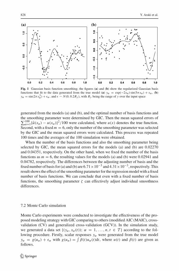
Figure 1 plots a set of 100 generated data from the model
(a) yα = exp(−2xα) sin(5πxα)+ εα, (b) yα = sin(2πx3α)+ εα,
where the errors εα are assumed to be independently distributed according to thenormal distribution with means 0 and the standard deviations are taken as 0.2Ry withRy being the range of (a) exp(−2xα) sin(5πxα) and (b) sin(2πx3
α), over the inputspace. The independent variable xα are generated from uniform distribution on [0, 1].
The solid lines are smoothed curves produced by using Gaussian basis func-tions, estimated by the regularization method. The number of basis functions andthe smoothing parameter ζ were selected by GIC in Eq. (11). The selected valueswere m = 6, ζ = 10−2.9, GIC = 46.35 for (a) and m = 4, ζ = 10−2.1, GIC = 93.66for (b).
Next we tried to adjust the smoothness of each curve by changing only the smooth-ing parameter, fixing the number of basis functions. First, 100 pairs of data were
123
828 Y. Araki et al.
1.00.0 0.2 0.4 0.6 0.8 1.0
-0.5
0.0
0.5
1.0
0.0 0.2 0.4 0.6 0.8 1.0
0.0
0.5
1.0
0.0 0.2 0.4 0.6 0.8 1.0
-1.5
-1.0
-0.5
0.0
0.5
1.0
(a) (b)
Fig. 1 Gaussian basis function smoothing; the figures (a) and (b) show the regularized Gaussian basisfunctions that fit to the data generated from the true model (a) yα = exp(−2xα) sin(5πxα) + εα, (b)yα = sin(2πx3
α)+ εα, and ε ∼ N (0, 0.2Ry), with Ry being the range of y over the input space
generated from the models (a) and (b), and the optimal number of basis functions andthe smoothing parameter were determined by GIC. Then the mean squared errors of∑100α=1{u(xα) − u(xα)}2/100 were calculated, where u(x) denotes the true function.
Second, with a fixed m = 6, only the number of the smoothing parameter was selectedby the GIC and the mean squared errors were calculated. This process was repeated100 times and the averages of the 100 simulation were obtained.
When the number of the basis functions and also the smoothing parameter beingselected by GIC, the mean squared errors for the models (a) and (b) are 0.02270and 0.04351, respectively. On the other hand, when we fixed the number of the basisfunctions as m = 6, the resulting values for the models (a) and (b) were 0.02941 and0.04782, respectively. The differences between the adjusting number of basis and thefixed number of basis for (a) and (b) are 6.71×10⁻³ and 4.31×10⁻³, respectively. Thisresult shows the effect of the smoothing parameter for the regression model with a fixednumber of basis functions. We can conclude that even with a fixed number of basisfunctions, the smoothing parameter ζ can effectively adjust individual smoothnessdifferences.
7.2 Monte Carlo simulation
Monte Carlo experiments were conducted to investigate the effectiveness of the pro-posed modeling strategy with GIC comparing to others (modified AIC (MAIC), cross-validation (CV) and generalized cross-validation (GCV)). In the simulation study,we generated a data set {(yα, xα(t)); α = 1, . . . , n, t ∈ T } according to the fol-lowing procedure. Firstly, scalar responses yα were generated from the true modelyα = g(uα) + εα with g(uα) = ∫ β(t)uα(t)dt , where u(t) and β(t) are given asfollows.
123
Functional regression modeling 829
(a) β(t) = t2, uα(t) = exp(a1αt)+ a2αt,
a1 ∼ N (2, 0.32), a2 ∼ N (−3, 0.42), T = [−1, 1], (58)
(b) β(t) = t2, uα(t) = b1α + b2αt + b3αt2 + b4αt3,
b1 ∼ N (0.2, 0.12), b2 ∼ N (0.4, 0.22), b3 ∼ N (0.1, 0.082),
b4 ∼ N (0.4, 0.12), T = [−1, 2]. (59)
The errors εα are assumed to be independently distributed according to the normaldistributions with means 0 and the variances are taken as (I) σ 2 = 0.01Rx , (II) σ 2 =0.05Rx with Rx being the range of g(uα) over the input space. Secondly, functionalpredictors xα(t) were generated as following steps:
Step 1. The design points {ti ; i = 1, . . . , 100} are generated independently fromuniform distribution on T .
Step 2. We obtain a discrete data set {(xαi , ti ); i = 1, . . . , 100, ti ∈ T }, wherexαi = uα(ti ) + eαi . The errors eαi are independently, normally distributedwith mean 0 and variance 1.
Step 3. The discrete data sets are transformed into a functional data set {xα(t); α =1, . . . , n} along with the smoothing technique described in Sect. 2.
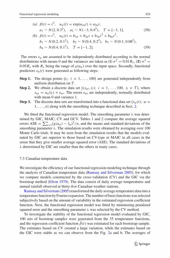
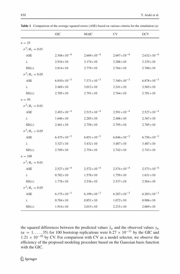
We fitted the functional regression model. The smoothing parameter λ was deter-mined by GIC, MAIC, CV and GCV. Tables 1 and 2 compare the average squarederrors ASE =∑n
α=1{g(uα)− yα}2/n, and the means and standard deviations of thesmoothing parameter λ. The simulation results were obtained by averaging over 100Monte Carlo trials. It may be seen from the simulation results that the models eval-uated by GIC are superior to those based on CV-type or MAIC in all cases in thesense that they give smaller average squared error (ASE). The standard deviations ofλ determined by GIC are smaller than the others in many cases.
7.3 Canadian temperature data
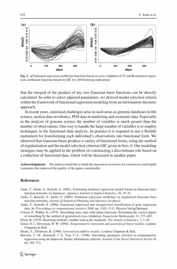
We investigate the efficiency of our functional regression modeling technique throughthe analysis of Canadian temperature data (Ramsay and Silverman 2005), for whichwe compare models constructed by the cross-validation (CV) and the GIC via thebootstrap method (Efron 1979). The data consist of daily average temperatures andannual rainfall observed at thirty-five Canadian weather stations.
Ramsay and Silverman (2005) transformed the daily average temperature data into atemperature function by Fourier expansion. The number of basis functions was selectedsubjectively based on the amount of variability in the estimated regression coefficientfunction. Next, the functional regression model was fitted by minimizing penalizedsquared error and the smoothing parameter λ was selected by the CV method.
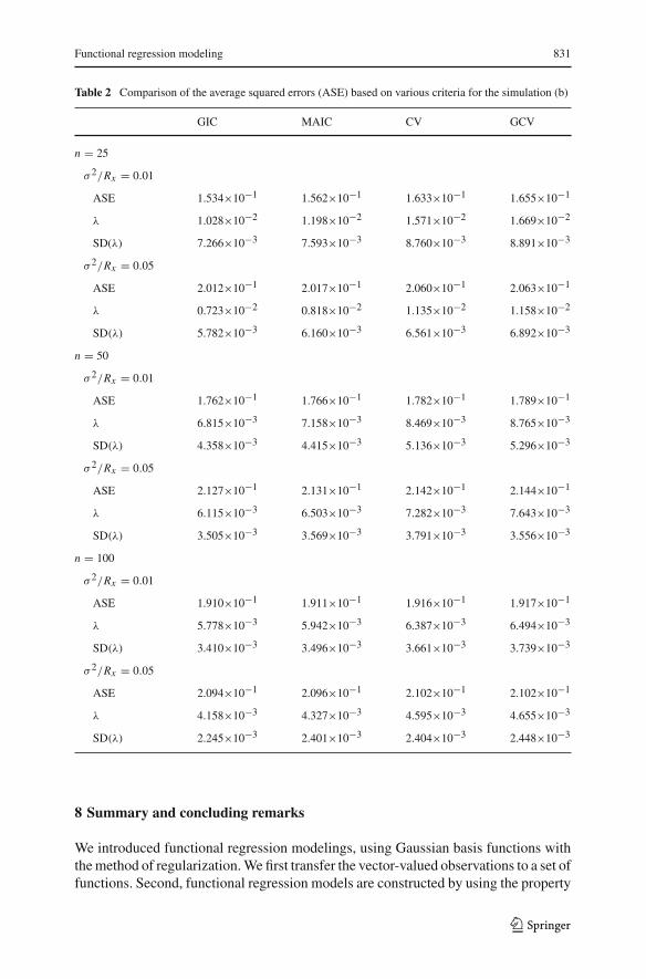
To investigate the stability of the functional regression model evaluated by GIC,100 sets of bootstrap samples were generated from the 35 temperature functions,and the regression coefficient function β(t) was estimated for each bootstrap sample.The estimates based on CV created a large variation, while the estimates based onthe GIC were stable as we can observe from the Fig. 2a and b. The averages of
123
830 Y. Araki et al.
Table 1 Comparison of the average squared errors (ASE) based on various criteria for the simulation (a)
GIC MAIC CV GCV
n = 25
σ 2/Rx = 0.01
ASE 2.548×10⁻⁴ 2.669×10⁻⁴ 2.697×10⁻⁴ 2.632×10⁻⁴
λ 2.934×10 3.174×10 3.288×10 3.335×10
SD(λ) 2.814×10 2.779×10 2.764×10 2.760×10
σ 2/Rx = 0.05
ASE 6.810×10⁻³ 7.371×10⁻³ 7.340×10⁻³ 6.878×10⁻³
λ 2.469×10 3.012×10 3.241×10 3.565×10
SD(λ) 2.705×10 2.791×10 2.764×10 2.701×10
n = 50
σ 2/Rx = 0.01
ASE 2.493×10⁻⁴ 2.515×10⁻⁴ 2.591×10⁻⁴ 2.527×10⁻⁴
λ 1.646×10 2.285×10 2.488×10 2.367×10
SD(λ) 2.461×10 2.758×10 2.795×10 2.785×10
σ 2/Rx = 0.05
ASE 6.475×10⁻³ 6.851×10⁻³ 6.846×10⁻³ 6.756×10⁻³
λ 3.327×10 3.432×10 3.487×10 3.487×10
SD(λ) 2.769×10 2.754×10 2.742×10 2.743×10
n = 100
σ 2/Rx = 0.01
ASE 2.527×10⁻⁴ 2.572×10⁻⁴ 2.574×10⁻⁴ 2.573×10⁻⁴
λ 0.782×10 1.578×10 1.759×10 1.631×10
SD(λ) 1.778×10 2.536×10 2.537×10 2.564×10
σ 2/Rx = 0.05
ASE 6.175×10⁻³ 6.199×10⁻³ 6.287×10⁻³ 6.203×10⁻³
λ 0.784×10 0.851×10 1.072×10 0.906×10
SD(λ) 1.914×10 2.015×10 2.215×10 2.069×10
the squared differences between the predicted values yα and the observed values yα(α = 1, . . . , 35) for 100 bootstrap replications were 6.27 × 10⁻¹¹ by the GIC and1.21 × 10−10 by CV. For comparison with CV as a model selector, we observe theefficiency of the proposed modeling procedure based on the Gaussian basis functionwith the GIC.
123
Functional regression modeling 831
Table 2 Comparison of the average squared errors (ASE) based on various criteria for the simulation (b)
GIC MAIC CV GCV
n = 25
σ 2/Rx = 0.01
ASE 1.534×10⁻¹ 1.562×10⁻¹ 1.633×10⁻¹ 1.655×10⁻¹
λ 1.028×10⁻² 1.198×10⁻² 1.571×10⁻² 1.669×10⁻²
SD(λ) 7.266×10⁻³ 7.593×10⁻³ 8.760×10⁻³ 8.891×10⁻³
σ 2/Rx = 0.05
ASE 2.012×10⁻¹ 2.017×10⁻¹ 2.060×10⁻¹ 2.063×10⁻¹
λ 0.723×10⁻² 0.818×10⁻² 1.135×10⁻² 1.158×10⁻²
SD(λ) 5.782×10⁻³ 6.160×10⁻³ 6.561×10⁻³ 6.892×10⁻³
n = 50
σ 2/Rx = 0.01
ASE 1.762×10⁻¹ 1.766×10⁻¹ 1.782×10⁻¹ 1.789×10⁻¹
λ 6.815×10⁻³ 7.158×10⁻³ 8.469×10⁻³ 8.765×10⁻³
SD(λ) 4.358×10⁻³ 4.415×10⁻³ 5.136×10⁻³ 5.296×10⁻³
σ 2/Rx = 0.05
ASE 2.127×10⁻¹ 2.131×10⁻¹ 2.142×10⁻¹ 2.144×10⁻¹
λ 6.115×10⁻³ 6.503×10⁻³ 7.282×10⁻³ 7.643×10⁻³
SD(λ) 3.505×10⁻³ 3.569×10⁻³ 3.791×10⁻³ 3.556×10⁻³
n = 100
σ 2/Rx = 0.01
ASE 1.910×10⁻¹ 1.911×10⁻¹ 1.916×10⁻¹ 1.917×10⁻¹
λ 5.778×10⁻³ 5.942×10⁻³ 6.387×10⁻³ 6.494×10⁻³
SD(λ) 3.410×10⁻³ 3.496×10⁻³ 3.661×10⁻³ 3.739×10⁻³
σ 2/Rx = 0.05
ASE 2.094×10⁻¹ 2.096×10⁻¹ 2.102×10⁻¹ 2.102×10⁻¹
λ 4.158×10⁻³ 4.327×10⁻³ 4.595×10⁻³ 4.655×10⁻³
SD(λ) 2.245×10⁻³ 2.401×10⁻³ 2.404×10⁻³ 2.448×10⁻³
8 Summary and concluding remarks
We introduced functional regression modelings, using Gaussian basis functions withthe method of regularization. We first transfer the vector-valued observations to a set offunctions. Second, functional regression models are constructed by using the property
123
832 Y. Araki et al.
0 100 200 300
-0.1
0-0
.05
0.0
0.05
0.10
0.15
days
Bet
a(t)
-0.1
0-0
.05
0.0
0.05
0.10
0.15
Bet
a(t)
0 100 200 300
days
(a) (b)
Fig. 2 a Estimated regression coefficient functions based on cross-validation (CV) and b estimated regres-sion coefficient functions based on GIC for 100 bootstrap replications
that the integral of the product of any two Gaussian basis functions can be directlycalculated. In order to select adjusted parameters, we derived model selection criteriawithin the framework of functional regression modeling from an information-theoreticapproach.
In recent years, statistical challenges arise in such areas as genome databases in lifescience, motion data in robotics, POS data in marketing and economic data. Especiallyin the analysis of genome science the number of variables is much greater than thenumber of observations. One way to handle the large number of variables is to employtechniques in the functional data analysis. In practice it is required to use a flexibleinstrument for transforming each individual’s observations into functional form. Weobserved that Gaussian bases produce a variety of functional forms, using the methodof regularization and the model selection criterion GIC given in Sect. 6. Our modelingstrategies may be applied to the problem of constructing a discriminant rule based ona collection of functional data, which will be discussed in another paper.
Acknowledgments The authors would like to thank the anonymous reviewers for constructive and helpfulcomments that improved the quality of the paper considerably.
References
Ando, T., Imoto, S., Konishi, S. (2001). Estimating nonlinear regression models based on Gaussian basisfunction networks (in Japanese). Japanese Journal of Applied Statistics, 30, 19–35.
Ando, T., Konishi, S., Imoto, S. (2005). Nonlinear regression modeling via regularized Gaussian basisfunction networks. Journal of Statistical Planning and Inference (in press).
Araki, Y., Konishi, S. (2006). Functional supervised and unsupervised classification of gene expressiondata. In: Proceedings in computational statistics 2006, pp. 1105–1112. Physica-Verlag/Springer.
Craven, P., Wahba, G. (1979). Smoothing noisy data with spline functions: Estimating the correct degreeof smoothing by the method of generalized cross-validation. Numerische Mathematik, 31, 377–403.
Efron, B. (1979). Bootstrap methods: another look at the Jackknife. The Annals of Statistics, 7, 1–26.Green, P. J., Silverman, B. W. (1994). Nonparametric regression and generalized linear models. London:
Chapman & Hall.Hastie, T., Tibshirani, R. (1990). Generalized additive models. London: Chapman & Hall.Hurvich, C. M., Simonoff, J. S., Tsai, C.-L. (1998). Smoothing parameter selection in nonparametric
regression using an improved Akaike information criterion. Journal of the Royal Statistical Society B,60, 359–373.
123
Functional regression modeling 833
James, G. (2002). Generalized linear models with functional predictor variables. Journal of the RoyalStatistical Society B, 64, 411–432.
Konishi, S., Kitagawa, G. (1996). Generalised information criteria in model selection. Biometrika,83, 875–890.
Kullback, S., Leibler, R. A. (1951). On information and sufficiency. Annals of Mathematical Statistics,22, 79–86.
Linhart, H., Zucchini, W. (1986). Finite sample selection criteria for multinomial models. Statistische Hefte,27, 173–178.
Marx, B. D., Eilers, P. H. C. (1999). Generalized linear regression for sampled signals or curves: A P-splineapproach. Technometrics, 41, 1–13.
Mizuta, M. (2006). Discrete functional data analysis. In: Proceedings in computational statistics 2006,pp. 361–369. Physica-Verlag/Springer.
Moody, J., Darken, C. J. (1989). Fast learning in networks of locally-tuned processing units. Neural Com-putation, 1, 281–294.
Nelder, J. A., Wedderburn, R. W. M. (1972). Generalized linear models. Journal of the Royal StatisticalSociety A, 135, 370–384.
Ramsay, J. O., Silverman, B. W. (2002). Applied functional data analysis. New York: Springer-Verlag.Ramsay, J. O., Silverman, B. W. (2005). Functional data analysis (2nd ed.). New York: Springer-Verlag.Rao, C. R., Wu, Y. (2001). Model selection. In: P. Lahiri (Ed.), Model selection: IMS lecture notes-
monograph series, pp. 1–18.Rice, J. A., Wu, C. O. (2001). Nonparametric mixed effects models for unequally sampled noisy curves.
Biometrics, 57, 253–259.
123