Juha Lahnakoski

Functional Magnetic Resonance Imaging of Human Brain during Rest and Viewing Movies

Faculty of Electronics, Communications and Automation

Master’s thesis submitted in partial fulfillment of the requirements for the degree of

Master of Science in Technology, Espoo 16.4.2010

Supervisor:

Professor Mikko Sams

Instructors:

Professor Mikko Sams, Professor Jouko Lampinen

AALTO UNIVERSITY MASTER’S THESIS

SCHOOL OF SCIENCE AND TECHNOLOGY ABSTRACT

Author: Juha Lahnakoski

Title: Functional Magnetic Resonance Imaging of Human Brain during Rest and

Viewing Movies

Date: April 16, 2010 Language: English Pages:8+51

Faculty of Electronics,Communications and Automation

Department of Biomedical Engineering and Computational Science

Professorship: Cognitive technology Code: S-114

Supervisor: Professor Mikko Sams

Instructor: Professor Mikko Sams , Professor Jouko Lampinen

Neuroscientific research of human brain function has traditionally relied on highly

controlled experiments with relatively simple stimuli. Recently effort has been directed

toward expanding the research into a more naturalistic context. Brain function has been

measured for example during viewing movies and in a ―resting state‖ in absence of as

specific task.

In this thesis, independent component analysis (ICA) is used to research human brain

function in naturalistic settings. The brain networks observed at rest are compared in

three conditions; resting before watching a movie (The Match Factory Girl, Aki

Kaurismäki, 1990), during the movie, and resting after the movie.

The stability of the source estimates obtained using ICA was evaluated using

bootstrapping. The temporal structure of the independent components (ICs) was

compared to stimulus features annotated from the movie. Similarity of the networks’

activation time courses across subjects was used to select components that were

compared with specific stimulus features. These features were also correlated directly to

the preprocessed data to validate the results of ICA.

ICA was successful at separating meaningful functional networks within the brain. The

extent of the networks changed very little between the different conditions. However,

the natural viewing condition allowed the ICs to be separated into smaller functional

units than was achievable during rest using both data-driven and model based methods.

The independent components exhibiting significant temporal similarity between

subjects were highly concentrated in the sensory and associative areas of the temporal,

occipital and parietal lobes. The activity of some ICs was found to follow distinct

features of the movie.

Keywords: Resting state, natural viewing, movie, brain, fMRI, ICA, correlation

iii

AALTO-YLIOPISTO DIPLOMITYÖ

TEKNILLINEN KORKEAKOULU TIIVISTELMÄ

Tekijä: Juha Lahnakoski

Työn nimi: Ihmisaivojen funktionaalinen magneettikuvantaminen levon ja elokuvien

katselun aikana

Päivämäärä: 16.4.2010 Kieli: Englanti Sivumäärä: 8+51

Elektroniikan, tietoliikenteen ja automaation tiedekunta

Lääketieteellisen tekniikan ja laskennallisen tieteen laitos

Professuuri: Kognitiivinen teknologia Koodi: S-114

Valvoja: Professori Mikko Sams

Ohjaaja: Professori Mikko Sams ja Professori Jouko Lampinen

Neurotieteellisissä kokeissa on perinteisesti käytetty tarkasti kontrolloituja koeasetelmia

ja yksinkertaisia ärsykkeitä aivojen toimintaa tutkittaessa. Viime aikoina tutkimusta on

pyritty laajentamaan luonnollisempiin asetelmiin. Aivojen toimintaa on mitattu

esimerkiksi koehenkilöiden katsellessa elokuvaa tai ‖lepotilassa‖ levollisen

valveillaolon aikana ilman mitään erityistä tehtävää.

Tässä diplomityössä tutkitaan ihmisen aivotoimintaa luonnollisen kaltaisissa tilanteissa

riippumattomien komponenttien analyysin (ICA) avulla. Lepotilassa löydettyjä

verkostoja verrataan kolmessa tilanteessa; levossa ennen elokuvan (Tulitikkutehtaan

tyttö, Aki Kaurismäki, 1990) katsomista, elokuvan aikana ja levossa elokuvan

katsomisen jälkeen jälkeen.

ICA:lla löydettyjen lähde-estimaattien vakautta tutkittiin bootstrap-laskennalla.

Elokuvasta annotoituja ärsykepiirteitä verrattiin niiden aivoverkostojen aikakäytökseen,

joiden aikakäyttäytyminen oli samankaltaista eri koehenkilöillä. Ärsykepiirteiden avulla

vertailtiin lisäksi ICA:n erottamien verkostojen laajuutta yksittäisten ärsykepiirteiden

kanssa korreloituviin aivoalueisiin.

ICA onnistui erottamaan merkityksellisiä toiminnallisia verkostoja aivoissa.

Verkostojen laajuudessa tapahtui vain vähän muutoksia eri koetilanteiden välillä.

Luonnollinen katselutilanne kuitenkin mahdollisti komponenttien jakamisen pienempiin

toiminnallisiin yksiköihin kuin lepotilassa sekä data-lähtöisin, että mallipohjaisin

analyysimenetelmin. Eri koehenkilöillä samankaltaisesti käyttäytyneet riippumattomat

komponentit paikantuivat lähinnä aistispesifeille ja assosiaatioalueille aivojen

temporaali-, oksipitaali- ja parietaalilohkoilla. Osalla komponenteista aikakäytöksen

havaittiin seuraavan elokuvasta annotoituja piirteitä.

Avainsanat: Lepotila, luonnollinen katselu, elokuva, aivot, fMRI, ICA, korrelaatio

iv

Foreword

This work was done as a part of a larger research project in the Department of

Biomedical Engineering and Computational Science at Aalto University School of

Science and Technology in collaboration with Department of Motion Picture,

Television and Production Design aiming to represent neuronal activity in the human

brain while watching natural movies.

I would like to thank Mikko Sams and Jouko Lampinen for excellent directions given

throughout the project. Thanks also to Juha Salmitaival for feedback on the thesis,

fellow thesis worker Jussi Nieminen for help and relaxed work atmosphere, and the

whole team involved in the current study for encouraging feedback and informative and

often entertaining meetings.

Most of all, thanks to my darling Sonja for love, encouragement and support.

v

Table of contents

ABSTRACT ...................................................................................................................... ii

TIIVISTELMÄ ................................................................................................................ iii

Foreword .......................................................................................................................... iv

Table of contents ............................................................................................................... v

Symbols and abbreviations ............................................................................................. vii

1 Introduction ............................................................................................................... 1

1.1 Nuclear magnetic resonance imaging (NMRI) .................................................. 2

1.2 Functional magnetic resonance imaging (fMRI) ............................................... 7

1.3 Independent component analysis (ICA) ............................................................. 9

1.4 Studying brain activity in naturalistic settings ................................................. 12

1.4.1 Default mode network .............................................................................. 14

1.4.2 Natural stimulation ................................................................................... 14

1.5 Aim of the study ............................................................................................... 16

2 Methods .................................................................................................................. 17

2.1 Subjects ............................................................................................................ 17

2.2 Procedure .......................................................................................................... 17

2.3 Imaging ............................................................................................................ 17

2.4 Software ........................................................................................................... 18

2.5 Data preprocessing ........................................................................................... 18

2.6 Movie annotation ............................................................................................. 19

2.7 Data analysis .................................................................................................... 20

2.8 Data representation ........................................................................................... 21

2.9 Component selection ........................................................................................ 22

3 Results ..................................................................................................................... 23

3.1 Independent components .................................................................................. 23

3.2 Spatial characterization of ICs in different conditions ..................................... 27

3.3 Temporal structure of the independent components ........................................ 28

3.3.1 Visual ICs ................................................................................................. 29

3.3.2 Auditory ICs ............................................................................................. 30

3.3.3 Parietal ICs ................................................................................................ 34

4 Discussion ............................................................................................................... 36

4.1 Conclusions ...................................................................................................... 39

5 Bibliography ........................................................................................................... 41

vi

Appendix A ..................................................................................................................... 47

vii

Symbols and abbreviations

Symbols

B Magnetic flux density

M Magnetization

T1 Spin-lattice relaxation time constant

T2 Spin-spin relaxation time constant

γ Gyromagnetic constant

μ Magnetic moment

ω Larmor frequency

Abbreviations

BOLD Blood Oxygenation Level-Dependent

CCA Curvilinear Component Analysis

DMN Default Mode Network

EPI Echo Planar Imaging

fALFF Fractional Amplitude of Low-Frequency Fluctuation

FDR False Discovery Rate

fMRI Functional Magnetic Resonance Imaging

FWHM Full Width at Half Maximum

HRF Hemodynamic Response Function

GLM General Linear Model

ICA Independent Component Analysis

IC Independent Component

IFG Inferior Frontal Gyrus

IPL Inferior Parietal Lobule

IPS Intraparietal Sulcus

MDL Minimum Description Length

MRI Magnetic Resonance Imaging

viii

MT Middle Temporal visual area (V5)

MTG Middle Temporal Gyrus

NMRI Nuclear Magnetic Resonance Imaging

PCA Principal Component Analysis

PFC Prefrontal Cortex

RF Radio Frequency

RMS Root Mean Square

RSN Resting State Network

TE Echo Time

TI Inversion Time

TR Repetition Time

SPL Superior Parietal Lobule

STG Superior Temporal Gyrus

STS Superior Temporal Sulcus

V5 See MT

1 Introduction

Functional Magnetic Resonance Imaging (fMRI) is a widely used method to study

various aspects of healthy and diseased brain [1]. In the majority of fMRI studies, well-

defined controlled stimuli have been used to activate the brain [2]. However, in the

present study the subjects watched a 23-minute long feature movie during fMRI

measurement. In two additional resting-state sessions, one before and one after the

movie, subjects lied wakefully resting in the scanner performing no specific task during

fMRI.

Model free analysis methods have provided tools for study of brain function in natural

conditions. Using independent component analysis (ICA) consistent cortical networks

have been extracted both during rest and during natural viewing [2; 3]. Additionally,

natural stimulation has been found to elicit highly synchronized activity in large areas of

the cerebral cortex [3; 4] allowing the brain function to be studied directly through inter-

subject correlations. Measures of inter-subject synchrony have also been applied to ICA

[5] to reveal networks of brain areas acting in unison between subjects.

So-called resting state activity has been examined in several studied. These studies have

found evidence of consistent resting state networks (RSN), which are thought to reveal

the functional organization of the brain [2; 6; 7]. Many resting state studies have

specifically concentrated on the so-called default mode network (DMN), which

deactivates during many cognitive tasks [8], while parts of the network activate while

watching social interactions [9] or thinking of moral dilemmas [10]. The functional

significance of DMN is not yet well known, but is often accredited to mind wandering

or underlying physiological processes [11]. Because coherent activation patterns are

obtained even during ―resting state‖, it has been questioned whether such periods in

fMRI studies can really be used as background activity for activated states [12]. There is

still quite little research done on how RSNs are modified during natural stimulation,

such as movies.

In the present work human cortical activity is studied using ICA. The stability of the

independent components (ICs) is assessed by bootstrapping, and the results are

validated by correlation analysis with features extracted from the movie. The

components included for temporal analysis are selected through their temporal

similarity between subjects. RSNs obtained in two sessions are compared to examine

their stability, and also how they may be modified by a movie watching task.

The fMRI study was done at Advanced Magnetic Imaging Centre (AMI Centre) of the

Aalto University School of Science and Technology. Activation was measured by

maximizing the contrast for the blood oxygen level-dependent (BOLD) signal [13],

which has been used extensively in previous fMRI studies .

2

1.1 Nuclear magnetic resonance imaging (NMRI)

Nuclear magnetic resonance imaging (NMRI) was first developed in the 1970s and

applied for structural imaging of the brain in the 1980s. It developed strongly during the

1990s as imaging sequences were developed allowing for a wide variety of contrast

methods, which in turn allowed for different aspects of the brain and body to be imaged

[14]. To set NMRI apart from invasive radiation based imaging modalities it is now

typically called just MRI to avoid misunderstandings [14].

The theory of MRI rests upon the fact, that all matter has an intrinsic magnetic property

called spin. Individual spins are magnetic field sources which interact with each other

and external magnetic fields. In an external magnetic field, unpaired spins in matter tend

to align themselves to the applied field (Fig. 1) [14] . Coincidentally the most abundant

molecule in the human body, water, carries two hydrogen atoms with such unpaired

spins making nuclear magnetic resonance imaging possible [14].

Figure 1: a) Spins of hydrogen nuclei in the absence of a magnetic field

may have any orientation. b) In external magnetic field spins arrange so

that they are either parallel (red) or anti-parallel (blue) to the external

field.

There are five separate sources of electromagnetic fields in a typical MRI scanner. The

main field is a static, and maximally uniform magnetic field, B0. Currently typical value

of B0 for medical use is either 1.5T or 3T for whole body scanners, but even stronger

field strengths are being used in research [15]. This strong magnetic field aligns all the

magnetic moments into direction either parallel or anti-parallel to itself, with a slight

majority of them being in the parallel direction. Only the slight excess of parallel spins

can be measured in the imaging process. In calculations, the direction of the static field

B0 is defined as the z-axis by convention [16].

The magnetization cannot be measured in the direction of the static magnetic field, and

therefore another field has to be introduced in the form of a coil, which is used to tip the

magnetization partially orthogonal to the field B0 [16]. To achieve this, a radio

3

frequency (RF) pulse is introduced to the system orthogonal to the direction of B0, the

amplitude and duration of which determines how much the magnetization is tipped; this

angle is generally called the flip angle [17]. The magnetic field of the RF pulse is

referred to as B1 in calculations and is typically sinusoid signal amplitude modulated by

a sinc-pulse which yields a rectangular profile in frequency domain. The same coils

used for the excitation pulse are typically also used for the data acquisition [16; 17].

The magnetic moments, μ, of the protons within the field B0 precess around the

direction of the field with an angular frequency ω, called the Larmor frequency, which

is proportional to the magnitude of the field (see Fig. 2) [16]. This is also the frequency

at which the RF pulse must be introduced, and gives the motivation for the third

component of the total magnetic field, which is a linear gradient over the area of

interest. This gradient causes the spins in different parts of the field to rotate at a slightly

different pace around the main field. If an RF pulse is introduced with a specific

frequency band, it targets only the protons with Larmor frequencies in that range. The

bandwidth of the pulse in frequency domain and the slope of the gradient determine the

thickness of the slice to be imaged, while the direction of the gradient determines the

imaging plane [16].

Figure 2: The magnetic moments (μ) of nuclei in a magnetic field precess

around the direction of the field B0 at Larmor frequency, ω.

To encode the other two dimensions two additional gradients are needed orthogonal

both to the slice selection gradient, and to each other. One is introduced before the

image acquisition causing the protons at different positions along one dimension to have

different phase angles when the image is acquired. The third gradient is applied during

data acquisition to encode the remaining direction on the slice with different frequencies

proportional to the strength of the gradient at each point [16].

The contrast in the acquired images arises from the way the magnetization (M) in the

tissue returns to its equilibrium state within the field B0. This process, called relaxation,

happens at different rates in different tissues. Relaxation happens by two different

ω

ω

μ

μ

4

mechanisms termed spin-lattice and spin-spin relaxation, which are governed by a set of

differential equations called the Bloch equations

(1a)

(1b)

(1c)

where γ is the gyromagnetic constant of the nucleus [16].

Spin-lattice relaxation, often called T1 relaxation, is the process through which the

z-component of the magnetization returns to its equilibrium value, and is governed by

the third equation. Spin-spin relaxation, also called T2 relaxation, governs how the

transverse magnetization returns to its equilibrium value of 0. Spin-spin relaxation

depends on two factors, pure T2 relaxation and T2+ relaxation. The pure T2 relaxation

arises from the loss of phase coherence between protons in the tissue, and T2+ is due to

spatial variations in the magnetic field. These spatial variations are mainly caused by

inhomogeneity of the magnetic field produced by the magnet and local changes in

magnetic susceptibility in the tissue. The total relaxation time constant of transverse

magnetism is termed T2*, and is given by

(2)

Imaging sequences used in MRI can be split into broad families of spin echo, and

gradient echo sequences. Different parameters governing the timing of the gradients can

be used to create different contrasts. A typical gradient echo sequence is presented in

Fig. 3a showing the gradients necessary for encoding each direction. Spin echo

sequence in Fig. 3b differs from the gradient echo sequence in that it employs an

additional 180˚ elctromagnetic refocusing pulse to compensate for the loss of phase

coherence after the excitation [17].

In typical anatomical imaging a single line within the two dimensional space of the

slice, called the k-space, is acquired with each phase encoding step. The time required

to acquire a single slice is governed by the time it takes to acquire each successive line

and the number of phase encoding steps. Typically a high quality anatomical image

acquisition takes several minutes [16].

5

Figure 3: a) Gradient echo pulse sequence showing the gradients at

different parts of the imaging process, and the data acquisition (DAQ). b)

Spin echo sequence depicting the imaging parameters TE and TR. Spin

echo sequence is characterized by the addition of a 180˚ refocusing pulse

at t=TE/2.

The basic parameters of repetition time, TR, and echo time, TE, govern the amount of

T1 and T2 weighting in the image, respectively. Repetition time determines the time

between successive excitation pulses, while echo time determines the time between

excitation and data acquisition (see Fig. 3b). When TE is short and TR is of

intermediate length, T1 contrast is maximized. When TR is made longer T1 contrast

diminishes, while increasing the echo time increases the T2 contrast until it reaches its

maximum and starts to decrease. By making the TR very long and TE very short both

T1 and T2 weighting are minimized and the contrast arises primarily from the density of

protons in the tissues. This method is called proton density imaging. Typical T1

recovery and T2 decay behavior of two different types of tissue after excitation is

depicted in Fig. 4, including the contrast between the two tissues. The optimal selection

of imaging parameters depends on the tissues to be imaged, and should be selected to

maximize the contrast between the tissues of interest [17].

To further increase the contrast of T1 weighted images, an inversion recovery sequence

may be used, in which the magnetization is inverted by a 180° RF pulse before

excitation. This effectively doubles the contrast present in the images because the

difference of the initial magnetization to the equilibrium state (Mz – M0) is twice as

large, which can be confirmed by applying equation 1c. Inversion recovery sequence

introduces a third parameter called inversion time (TI), which determines the time

between the inversion and excitation pulses [17].

6

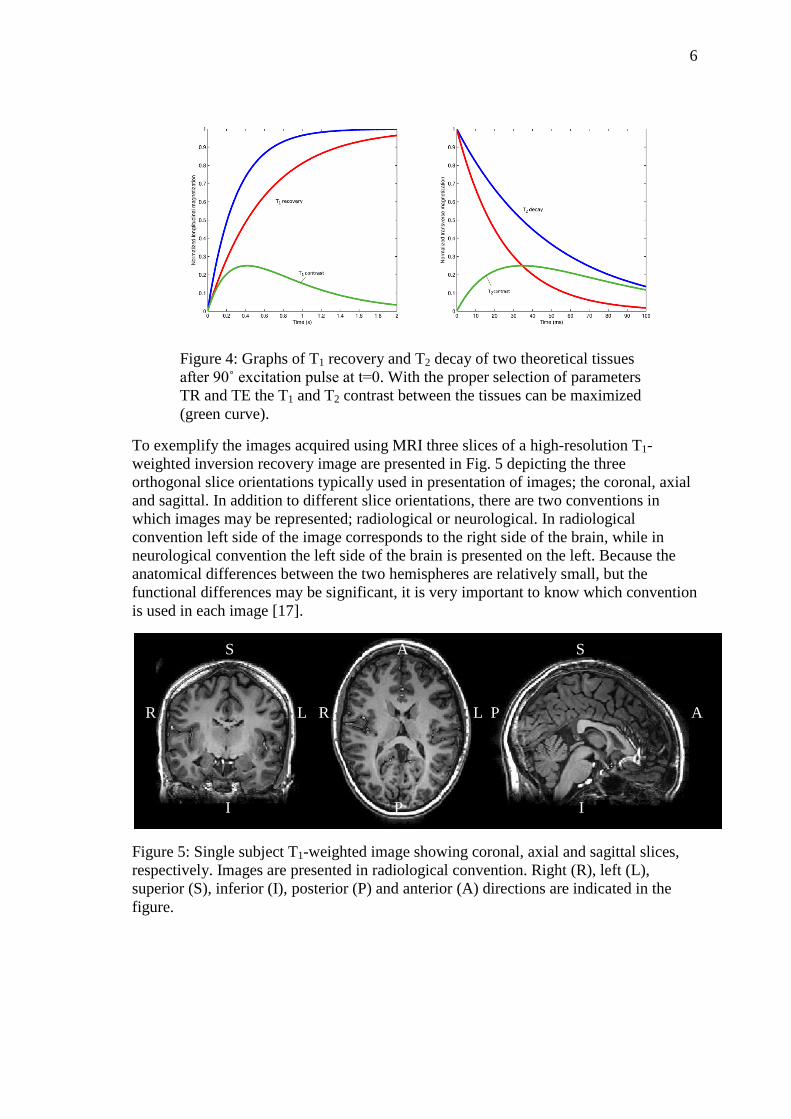
Figure 4: Graphs of T1 recovery and T2 decay of two theoretical tissues

after 90˚ excitation pulse at t=0. With the proper selection of parameters

TR and TE the T1 and T2 contrast between the tissues can be maximized

(green curve).

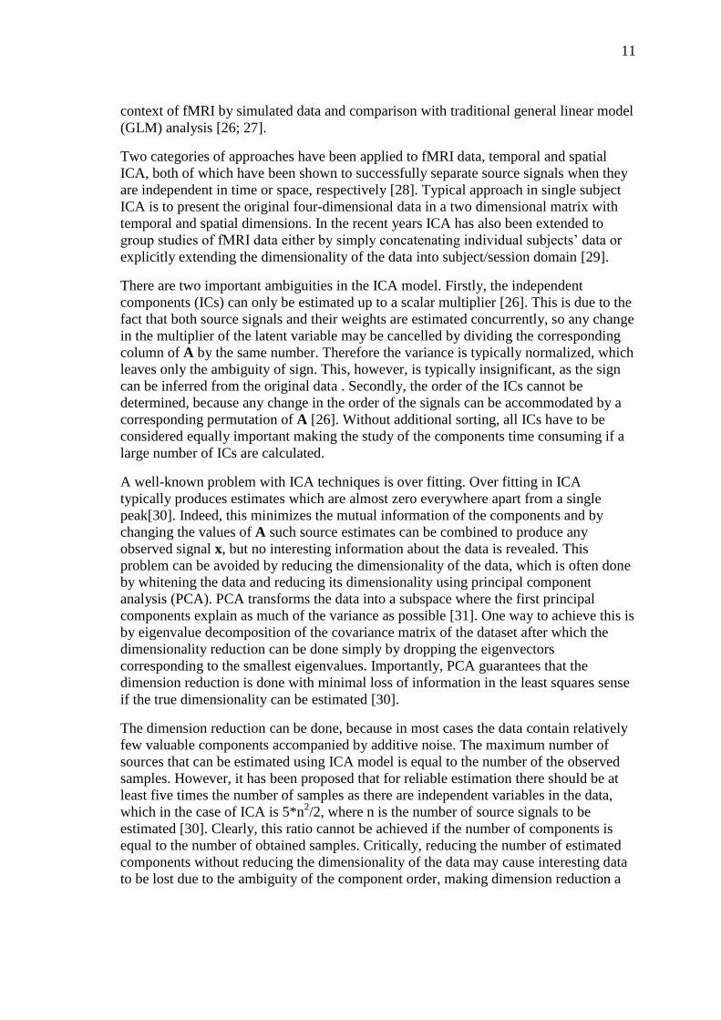
To exemplify the images acquired using MRI three slices of a high-resolution T1-

weighted inversion recovery image are presented in Fig. 5 depicting the three

orthogonal slice orientations typically used in presentation of images; the coronal, axial

and sagittal. In addition to different slice orientations, there are two conventions in

which images may be represented; radiological or neurological. In radiological

convention left side of the image corresponds to the right side of the brain, while in

neurological convention the left side of the brain is presented on the left. Because the

anatomical differences between the two hemispheres are relatively small, but the

functional differences may be significant, it is very important to know which convention

is used in each image [17].

Figure 5: Single subject T1-weighted image showing coronal, axial and sagittal slices,

respectively. Images are presented in radiological convention. Right (R), left (L),

superior (S), inferior (I), posterior (P) and anterior (A) directions are indicated in the

figure.

S A S

R L R L P A

I P I

7

1.2 Functional magnetic resonance imaging (fMRI)

Functional magnetic resonance imaging has surfaced as possibly the most important set

of functional brain imaging techniques for neuroscientific research in the recent years.

At present, it is used extensively to record differences occurring in the magnetic

susceptibility of brain regions as a result of neural activation.

Same equipment used for structural imaging can be utilized for functional imaging by

proper selection of parameters. As mentioned in the last chapter, different magnetic

susceptibilities cause changes in the T2* relaxation times through the T2

+ component in

equation 2. In practice the T2* relaxation may be up to 10-100 times faster in tissue, than

pure T2 relaxations [16].

To allow imaging of brain function, fast imaging sequences must be used. The most

popular is the echo planar imaging (EPI) sequence, depicted in Fig. 6, which allows the

whole k-space of the slice to be acquired with a single excitation, and series of

successive phase and frequency encoding steps during simultaneous data acquisition

[17]. This allows the whole k-space to be recorded in less than 100ms. However, fast

imaging sequences often require trade-offs to be made between the image contrast and

spatial and temporal resolutions due to the time constants governing the magnetic

relaxation [16; 18].

Figure 6: a) Echo Planar Imaging (EPI) pulse sequence. Whole k-space

is covered with one excitation pulse followed by multiple phase and

frequency encoding steps by fast switching of gradients during

concurrent data acquisiton. b) EPI k-space trajectory. Imaged line is

switched with the phase encoding gradients (dotted line) while each line

is imaged during the frequency encoding gradients in alternating

directions.

The most prevalent technique for recording brain activity is through the changes in

Blood Oxygen-Level Dependent (BOLD) signal introduced in 1988 by Ogawa and

co-workers [13]. The underpinning of this technique is that the energy consumption of

activated neurons rises, increasing oxygen consumption of the activated cells. This leads

to an increase in cerebral blood flow to the activated area. However, the increase of

8

blood flow over compensates for the rise in oxygen consumption. This results in an

increase of oxygenated hemoglobin in the activated area lowering the deoxyhemoglobin

concentration in the region. Because deoxygenated hemoglobin is paramagnetic, unlike

the oxygenated variant, the lower concentration decreases the local magnetic

susceptibility therefore reducing the dephasing of the spins in the area. This shows in

the T2* weighted fMRI images as an amplified signal at the corresponding region of the

brain. The local changes in susceptibility are barely visible in spin echo imaging

sequences and therefore gradient echo sequences must be used [17]. Other contrast

techniques have also been used for functional MRI e.g. tracking cerebral blood flow

through exogenous contrast agents and arterial spin labeling, but these methods are

currently less popular [14; 19].

The underlying causes of BOLD signal are still uncertain. The mechanism triggering the

increase in blood flow responsible for the BOLD signal has been hypothesized to be

caused by presynaptic activity and neurotransmitter cycling predicting the increase of

energy consumption rather than the energy consumption directly. However, while

presynaptic processes may trigger the increase in blood flow, the majority of the energy

consumption is attributed to the postsynaptic potentials. Therefore, the BOLD signal

primarily reflects the information processing in neurons rather than the signals

transmitted by action potentials in the axon. The reason for the mismatch in oxygen

supply and consumption causing the signal is also unclear. One possibility is that the

blood contains a constant ratio of blood and glucose and the blood flow is governed by

the supply of glucose, which more closely follows the demand of the cells. An

alternative hypothesis attributes the mismatch to inefficient oxygen delivery process

[20].

The BOLD signal change following the activation is called the hemodynamic response

[17]. The hemodynamic response is typically approximated through a canonical

hemodynamic response function (HRF) approximating the BOLD response to a short

stimulus. A typical HRF is presented in Fig. 7a. It begins with an initial undershoot,

which is not modeled in all canonical HRFs and is not seen in all practical experiments.

The cause of this undershoot is uncertain, but it has been hypothesized to be caused by

the rise in oxygen consumption before the blood flow reaches the activated area [21].

After the initial dip, the signal starts to rise as more blood reaches the site of activation.

The signal reaches its peak when the amount of oxygenated blood is at maximum,

typically between 4 and 6 seconds of the activation depending on the subject and the

area of the brain. After this, if no further activation is triggered, the blood level starts to

drop and an additional undershoot is observed after approximately 10 seconds after the

initial activation. If the activation continues the BOLD signal drops slightly to a

saturation level after the initial peak. The hemodynamic response caused by a

continuous activation can be mathematically represented by a convolution of the

canonical HRF and the underlying activity, and is depicted in Fig. 7b [17]. While this

linear model of hemodynamic activity is not strictly accurate, it is however used in

many data analysis packages as a useful approximation [20].

9

Figure 7: Shape of the hemodynamic response to (a) a short stimulus and

(b) 62.5 seconds of continuous stimulation.

There are major challenges in using BOLD signals as a marker for neural activity. For

example, there are various non-neuronal sources of BOLD signal in different parts of

the brain, often called artifacts, which must be identified from the data. Typical sources

of artifacts include head motion, respiration and cardiac rhythm. In general artifacts

have a signature that differs from the signals of interest, and they can be automatically

separated to some degree by filtering or independent component analysis for example

[22; 23].

Other challenges relate to the properties of the BOLD signal itself. The changes in local

susceptibility caused by neuronal activity exert relatively small changes in the recorded

signal, which requires powerful statistical methods for extracting the features of interest

from the baseline signal. Additionally, the differences in the onset time of the

hemodynamic response may be in the order of seconds between different areas of the

brain. This leads to ambiguity in the recorded time domain signals making it difficult to

draw clear-cut conclusions of functional relationships between brain areas [1].

The regional differences in the HRF can be eliminated to some degree by deconvolution

techniques, if the local HRFs can be estimated or measured accurately. In a recent study

done on rats the neural drivers of non-convulsive epilepsy were correctly distinguished

in the barrel field of the primary somatosensory cortex when the effects of HRF were

explicitly removed from the fMRI signal [24]. The estimation of local the HRF is

especially important in model-based methods, where the model fit is directly dependent

on the accuracy of the HRF estimate. Different techniques have been proposed to

estimate the HRF in humans, including Bayesian methods, and independent component

analysis [25]. Additionally, statistical methods like the dynamic causal modeling

(DCM) approach have been developed for finding the sources of modulations within the

brain despite the differences in regional delays [1].

1.3 Independent component analysis (ICA)

Independent Component Analysis is a relatively recent a blind source separation

technique which has been applied to a wide range of disciplines [26]. In fMRI, ICA has

been used mainly in naturalistic settings, especially in resting state studies, where no

10

models exist for the spontaneous neuronal activity. Additionally ICA has proved useful

in denoising the fMRI signal by removing artifact [22].

The ICA framework assumes that the observed signals are composed of an unknown

mix of source signals, which are treated as latent random variables, and cannot be

observed directly. The goal of the method is to estimate both the source signals and

their relative weights from the observed samples [26]. Fig. 8 illustrates this by an

example where six different mixes of two images are subjected to ICA. The estimated

independent components in this noise free example are essentially identical to the

original images, with no visible degradation of image quality.

The ICA mixing model can be expressed formally by the equation

, (3)

where is the matrix of observed samples in its columns, is the matrix of weights of

the source signals, and is the matrix containing the source signals to be estimated in

its columns [26].

Figure 8: Example of ICA: Original images to be estimated are mixed

into six composite images. ICA finds the independent components

corresponding to the original images from the composites. FastICA

algortihm with gauss nonlinearity was used for the separation.

The basis of ICA is in the assumption that the source signals are statistically

independent and their distributions are non-Gaussian. With these restrictions contrast

functions may be created, which allow independent source signals to be extracted [26].

Several different algorithms have been created to implement ICA, which have different

optimization criteria for the source estimates. Typical ICA algorithms achieve the

independence of components by minimizing the mutual information of individual

source estimates, while the practical approaches to this may be somewhat different. For

example, information maximization and maximization of the non-Gaussianity of

component estimates have been used, which are the approaches taken by the two most

widely employed algorithms in fMRI signal analysis, Infomax and FastICA [26],

respectively. Both are iterative algorithms and produce highly similar results. They

produce consistent estimates across different runs, and have been validated in the

11

context of fMRI by simulated data and comparison with traditional general linear model

(GLM) analysis [26; 27].

Two categories of approaches have been applied to fMRI data, temporal and spatial

ICA, both of which have been shown to successfully separate source signals when they

are independent in time or space, respectively [28]. Typical approach in single subject

ICA is to present the original four-dimensional data in a two dimensional matrix with

temporal and spatial dimensions. In the recent years ICA has also been extended to

group studies of fMRI data either by simply concatenating individual subjects’ data or

explicitly extending the dimensionality of the data into subject/session domain [29].

There are two important ambiguities in the ICA model. Firstly, the independent

components (ICs) can only be estimated up to a scalar multiplier [26]. This is due to the

fact that both source signals and their weights are estimated concurrently, so any change

in the multiplier of the latent variable may be cancelled by dividing the corresponding

column of A by the same number. Therefore the variance is typically normalized, which

leaves only the ambiguity of sign. This, however, is typically insignificant, as the sign

can be inferred from the original data . Secondly, the order of the ICs cannot be

determined, because any change in the order of the signals can be accommodated by a

corresponding permutation of A [26]. Without additional sorting, all ICs have to be

considered equally important making the study of the components time consuming if a

large number of ICs are calculated.

A well-known problem with ICA techniques is over fitting. Over fitting in ICA

typically produces estimates which are almost zero everywhere apart from a single

peak[30]. Indeed, this minimizes the mutual information of the components and by

changing the values of A such source estimates can be combined to produce any

observed signal x, but no interesting information about the data is revealed. This

problem can be avoided by reducing the dimensionality of the data, which is often done

by whitening the data and reducing its dimensionality using principal component

analysis (PCA). PCA transforms the data into a subspace where the first principal

components explain as much of the variance as possible [31]. One way to achieve this is

by eigenvalue decomposition of the covariance matrix of the dataset after which the

dimensionality reduction can be done simply by dropping the eigenvectors

corresponding to the smallest eigenvalues. Importantly, PCA guarantees that the

dimension reduction is done with minimal loss of information in the least squares sense

if the true dimensionality can be estimated [30].

The dimension reduction can be done, because in most cases the data contain relatively

few valuable components accompanied by additive noise. The maximum number of

sources that can be estimated using ICA model is equal to the number of the observed

samples. However, it has been proposed that for reliable estimation there should be at

least five times the number of samples as there are independent variables in the data,

which in the case of ICA is 5*n2/2, where n is the number of source signals to be

estimated [30]. Clearly, this ratio cannot be achieved if the number of components is

equal to the number of obtained samples. Critically, reducing the number of estimated

components without reducing the dimensionality of the data may cause interesting data

to be lost due to the ambiguity of the component order, making dimension reduction a

12

necessity. This is demonstrated by an example in Fig. 9 with the same images as before

using FastICA algorithm with a limit on the number of ICs with no dimension

reduction.

Figure 9: Two independent components obtained by two separate runs of

FastICA without dimension reduction. Due to ambiguity of component

order, images can be lost completely in some runs if number of ICs is

reduced without dimension reduction (a), while on other runs both are

found (b).

Different schemes have been proposed for the important task of dimension estimation,

but no single approach has been uniformly adopted. Many of the previously used

methods have been shown to yield unreliable results in the presence of correlated noise

or when the data have been smoothed which renders the voxel data statistically

dependent and limits the usefulness of information theoretic model selection criteria. A

correction technique for the inherent sample dependence in fMRI was recently proposed

to mitigate the problem and has been adopted in the Group ICA fMRI Toolbox used in

the current study [32]. In addition to the aforementioned problem, some of the methods

currently in use appear to show almost linear relation for number of estimated

components and number of samples in the dataset, which has been criticized as

unrealistic [32; 33].

1.4 Studying brain activity in naturalistic settings

Model free exploratory analysis techniques like ICA make it possible to study human

brain functions in natural settings like during relaxed rest and perceiving complicated

time-varying natural stimuli. Additionally, measuring inter-subject synchrony can be

used to reveal brain areas undergoing similar activation in different subjects during

natural viewing of complex stimuli such as movies [6; 3; 34; 35; 36].

Studying patterns of brain activity in natural conditions poses many challenges. A major

challenge in analysis of fMRI data during resting state is separating neural BOLD

signals from other sources of low frequency signals, like heart beat and respiration,

which have been shown to cause significant signal changes not only near large blood

vessels, but also throughout grey matter [37; 38]. While most of the noise sources have

different frequency content than the neural activations, they may be aliased to lower

frequencies in the sampling process, and some noise is naturally present in the same

frequency range that is studied in resting state analysis [37]. Therefore simple frequency

based filtering is not enough to separate noise components from the signal. ICA has

been used [22] to separate activity of interest from noise sources. However, care has to

be taken to verify the identified components because valuable data may otherwise be

lost.

13

In typical fMRI experiments a block design is used with periods of control state and

periods of activity. In an experiment of this kind, the physiological and scanner related

noise is not correlated with the block design, and therefore the cerebral response to the

task can be separated by averaging multiple repetitions of the task and control states.

However, these types of experiments typically target only the areas specifically

activated by the task. They may therefore overlook areas active during rest despite they

may be crucial to the task performance [12]. Additionally, the resting state of the brain

is somewhat ill-defined as it can vary both within and between subjects [39].

Measuring fMRI during resting state is a relatively new field, the feasibility of which

was first demonstrated by Biswal and co-workers in 1995. By studying correlations of a

seed voxel in the motor cortex across the brain, they found the seed voxel correlated

only with other voxels in the motor cortex in absence of task [6; 40]. This

synchronization of brain areas is often called functional connectivity, because it is

thought to reveal their functional relations [7]. Typically, functional connectivity

analyses rely on selection of specific seed regions. However, the selection of a seed

region is problematic. To alleviate this problem, a method using spectral coherence

across brain regions has been proposed [41].

Traditional experiment design cannot be applied to resting state studies because there is

no control state to which the rest condition can be compared. Additionally, without

knowledge of the activation patterns, there is no possibility for averaging out any

uncorrelated noise as the signals of interest themselves are uncorrelated between

sessions and subjects. Therefore, several model free methods have been applied to

resting state studies such as clustering [36], fractional amplitude of low-frequency

fluctuations (fALFF) [7], PCA [42] and ICA [2; 7].

There has been much debate on the interpretation of the findings obtained. Using ICA

several researchers have found low frequency activation patterns consistent with areas

of functional specialization in the brain in the absence of a specific task [2; 6].

However, there is lack of evidence whether these patterns are due to either neural

activity, or oxygenation changes due to underlying physiology such as blood flow in

blood vessels feeding the brain areas [37].

There is general agreement that resting state patterns are present at low frequencies,

approximately in the range of 0.1 Hz – 0.01Hz [2; 6; 37]. This frequency band is the

main target of interest in this study.

Several RSNs have been reported in literature, which follow functionally specific areas.

In addition to the motor cortex, areas such as the visual and auditory cortices have been

segregated into separate RSNs [43; 44]. These networks are thought to reveal the

underlying organization of the brain, and can be found in absence of a task specifically

activating these areas [6; 7; 36]. Recent multisite study covering over 1400 subjects

identified twenty consistent RSNs present in the low frequency-range [7]. However,

these included all the consistent physiological artifacts, such as the fluctuations within

the ventricles.

14

1.4.1 Default mode network

The majority of resting state studies in the past has concentrated on the so-called default

mode network (DMN), which has been observed to show deactivation during many

cognitive tasks [38]. Some studies have used this task related deactivation directly to

separate areas of the DMN [37; 38]. However, other studies have shown increased

activity in parts of this network, e.g. when watching social interactions [9]. The DMN

has been reported to consist of posterior cingulate cortex, precuneus, medial prefrontal

cortex and bilateral inferior parietal cortex. However, there are differences in the sizes

of the areas from one study to the next [2; 6; 44].

Two classes of theories have been proposed for the cause of the activity within the

DMN [11]. First class states, that DMN takes part in spontaneous, intrinsic functions

reflecting unconstrained thought processes or physiological functions independent of

conscious mental activities. Second class relates these regions to ongoing and recent

experiences taking part in such activities as encoding the preceding situations into

memory [11].

Functional connectivity has received a lot of interest in resting state analysis. Many

studies have specifically examined the functional connectivity of the precuneus and

posterior cingulate area of the DMN to other regions of the brain. This cluster is

proposed to play a pivotal role in the DMN due to its strong connectivity to all other

nodes of the network [8; 11]. Modifications in connectivity of the cluster have been

reported not only during task but also lasting several minutes after the task has ended

[11]. Additionally, increased activity of the network has been reported to predict

successful memorization of informative sentences [45]. This has been proposed to

support the theory, that the network indeed takes part in processing conscious

experiences, especially coding recent experiences into memory [11]. Additionally,

changes in the areas of the network nodes have also been reported to depend on

particular task demands, while their locations stay remarkably similar [10]. Specifically,

moral dilemma tasks were shown to elicit correlated activity in larger cortical areas

around all nodes of the network, than was observed during rest. Conversely, smaller

correlated areas were observed during Stroop color-word interference task [10].

The theory relating DMN activity unconstrained intrinsic functions is supported by

observations of similar network in primates, and several states of unconsciousness in

humans [11; 46]. This is proposed to demonstrate, that functions other than conscious

thoughts are, at least in part, responsible for the observed coherent fluctuations in the

network [46]. Recently, changes in the connectivity strength and fluctuation amplitudes

in different areas of the network were also related to the age and sex of the subjects [7].

1.4.2 Natural stimulation

The study of human brain function during natural stimulation has increased in the last

few years. Different approaches have been used to move toward natural stimulation.

Some studies have used combinations of natural stimulation and block design to

validate the use of model free methods. Results of ICA have been succesfully related to

speech, and videos of faces and hands [47], and verified using general linear modeling

15

(GLM). Driving speed during simulated driving experiment has been related to

deactivations in ICs in the orbitofrontal and anterior cingulate cortices [48] when ICs

were selected through task relatedness in a block design including periods of fixation,

driving and watching. The use of inter-subject correlation has also been validated in

traditional experiments [49], where it uncovered task related areas not found by

traditional methods.

Recently, natural movies have often been used to approximate real life situations. While

movies also lack the well defined, unchanging block structure used in traditional

experiments, they can still be presented unchanged multiple times to multiple subjects.

Additionally, different features, such as visual motion, can be extracted from the

stimulus, and compared to the activity in different areas of the brain [4; 50].

Natural stimulation may provide a useful, less restricted context that still causes reliable

and highly synchronized activity in many brain areas across subjects [4]. Natural

conditions reveal activity patterns that are difficult if not impossible to discover by

traditional methods. The extent of the reliably activated areas appears to depend on the

presented stimulus. Early research [35] employing a measure of inter-subject correlation

identified only sensory and associative areas in the temporal, occipital and parietal

lobes. However, when subjects watched the last 36 minutes of a movie during fMRI

after seeing the beginning outside of the scanner [3] synchronization was also observed

in the prefrontal cortex. Recently, Hasson and co-workers [4] directly compared the

extent of inter-subject synchronization due to different types of videos; a segment of

real life, a silent film, an episode of a television show, and segment of a movie. They

found the structured videos elicited reliable activity in extensive areas of the brain,

while only areas of the early visual and auditory systems synchronized while watching

real life segments. Differences between the more structured videos were also reported.

The extent of the synchronized areas may depend on various factors. For example, the

synchronization of the prefrontal cortex may be due to subjects becoming emotionally

engaged in the movie through following the plot or due to techniques used by the

director to exert control on the audience [3; 51].

The functional specialization of brain areas has been studied in natural conditions using

ICA, which has been shown to separate several consistent components with highly

synchronized activation time courses between multiple subjects. Often the studies have

concentrated on visual and auditory areas, however, networks unrelated to the stimulus

have also been reported [3; 47], which are very similar to those reported in resting state

studies.

Bartels and Zeki [5] demonstrated that meaningful, functionally distinct networks can

be identified through their temporal characteristics without any prior knowledge of their

functional significance. They compared the activity in networks separated by ICA both

within subject and between subjects. More areas with characteristic activation patterns

were separated in the natural setting than were found in an experiment employing a

traditional block paradigm, and time courses of many ICs were highly similar between

subjects. Their findings support the notion that natural stimulation may assist in

observing patterns of activation, which would be difficult to study in a controlled

setting.

16

In an earlier study, Bartels and co-workers [34] analyzed functional connectivity of

areas segregated by ICA. Two specific regions with known anatomical connections

were studied; the language network in the left hemisphere, and areas of the visual

cortex. They found that directly connected regions exhibited stronger connectivity

during natural stimulation than at rest, while the connectivity of non-connected areas

decreased. They concluded that functional connectivity yields more robust estimates of

anatomical connectivity during natural viewing than at rest.

1.5 Aim of the study

There were two aims for the current study. First, to study the spatial modulation of ICs

separated in three conditions; resting before the movie, during the movie and resting

after the movie. Second, the temporal behavior of ICs during the movie condition was

to be studied. Measures of consistency of activation for different subjects, and

consistency of estimates in multiple repetitions were chosen to validate the ICs.

Additionally, the anatomical plausibility of the ICs was considered in selecting the ICs

to be examined.

The hypotheses of the current study were that ICA can be used to extract meaningful

networks of activity, and that these networks participate in processing the natural

stimulus. From prior research [4] it was expected, that the activity during natural

viewing is highly similar for different individuals in large areas of the cerebral cortex,

and that the synchrony can also be observed in the ICs separated by ICA [5]. It was

further hypothesized that features extracted from the movie can be used to predict

activity patterns of ICs.

17

2 Methods

2.1 Subjects

Ten healthy, Finnish speaking subjects were studied (two female, two left-handed).

Subjects’ ages ranged from 22 to 43 years (mean age 30.3, standard deviation 5.98).

Permission for the study was acquired from the ethical committee of Hospital district of

Helsinki and Uusimaa. The study was carried out in accordance with the guidelines of

the declaration of Helsinki, and informed written consent was obtained from each

subject prior to participation.

2.2 Procedure

Subjects were studied in three conditions. In the first ―resting state‖ condition subjects

only task was to fixate on a stationary cross stimulus for 15 minutes. In the second

―movie‖ condition, the subjects were presented the first 22 minutes 58 seconds of a

feature movie (re-edited version of The Match Factory Girl, Aki Kaurismäki, 1990).

Subjects were instructed to lie still, watch the movie and react to it normally. Second

resting state session, identical to the first session was recorded after the movie. Both the

movie and the static fixation stimuli were controlled using Presentation

(Neurobehavioral Systems Inc., Albany, California, USA) and projected on a

semitransparent screen using a 3-micromirror data projector (Christie X3, Christie

Digital Systems Ltd ., Mönchengladbach, Germany). The subjects viewed the screen at

34 cm viewing distance via a mirror located above their eyes. Audio track of the movie

was played using pneumatic headphones attached to earplugs in the subjects’ ears.

2.3 Imaging

Functional brain imaging was carried out with a 3.0 T GE Signa Excite MRI scanner

(GE Medical Systems, USA) using a quadrature 8-channel head coil. The imaging area

consisted of 29 functional gradient-echo planar (EPI) axial slices (thickness 4 mm,

between-slices gap 1 mm, in-plane resolution 3.4 mm x 3.4 mm, voxel matrix 64 x 64,

TE 32 ms, TR 2000 ms, flip angle 90°). Functional images were acquired continuously

during the experiment. In addition, a T1-weighted inversion recovery spin-echo volume

was acquired for anatomical alignment (TE 1.9 ms, TR 9 ms, flip angle 15°). The T1

image acquisition used the same slice prescription as the functional image acquisition,

except for a denser in-plane resolution (in-plane resolution 1 mm x 1 mm, matrix 256 x

256) and thinner slice thickness (1mm, no gap).

Each resting state condition consisted of 450 functional volumes and 689 volumes were

acquired in the movie condition.

18

2.4 Software

ICA was performed using two software packages, FMRIB Software Library (FSL) and

Group ICA of fMRI Toolbox (GIFT).

FMRIB Software Library (FSL) is comprehensive set of tools for various stages of

fMRI data processing and analysis. It has tools for most of the preprocessing steps

necessary for fMRI data analysis including, for instance, brain extraction, noise

reduction, motion correction. References for the FSL tools and analysis methods are

available at fMRIB Software Library’s WWW page (http://www.fmrib.ox.ac.uk/fsl/)

[52; 53; 54]. In the current study, FSL was used for preprocessing and analysis of the

single subjects’ datasets. The version used in this study was FSL 4.1.4.

GIFT is a toolbox for MATLAB mathematics software suite. It offers various features

to extend independent component analysis to the study of groups of subjects and

sessions, and a wide array of algorithms for independent component analysis. These

include the popular FastICA and Infomax, and several others. In addition GIFT has

included ICASSO software [55] for investigation of the reliability of source estimates,

which is a very useful tool in evaluating each ICA algorithm. The version used in the

creating the final results of this study was GIFT v1.3g.

Correlation analysis, and IC thresholding were performed using MATLAB 7.8.0 (The

MathWorks, Inc. 2009). For loading data in MATLAB, a package called NIfTI tools by

Jimmy Shen of Rotman Research Institute was used (http://www.rotman-baycrest.on.ca/

~jimmy/NIFTI/).

The ICs and correlation maps presented in this document were created using MRIcroN

by Chris Rorden of Georgia Institute of Technology (http://www.cabiatl.com/mricro/),

excluding the single subjects’ correlation maps (Fig. 19) and images in Appendix A,

which were exported directly from MATLAB.

2.5 Data preprocessing

All the preprocessing steps were performed using FEAT (FMRI Expert Analysis Tool)

Version 5.98, part of FSL (FMRIB’s Software Library). Motion correction was applied

using MCFLIRT, and non-brain matter was removed using BET (Brain Extraction

Tool). Values for intensity threshold and threshold gradient in BET were searched

manually by changing the parameters and visually checking each brain extracted

volume until the results were satisfactory. The datasets were registered to 2mm MNI152

standard space template using the brain extracted T1 weighted image of each individual

subject as an intermediate step for greater accuracy using FLIRT (FMRIB’s Linear

Image Registration Tool). Registration was performed using the default parameters with

12 degrees of freedom. Standard space data were smoothed using a Gaussian kernel

with full width at half maximum (FWHM) of 10.0 mm. The entire 4D datasets were

intensity normalized by a single multiplicative factor. High-pass temporal filtering was

applied using Gaussian-weighted least-squares straight line fitting, with sigma 100.0s.

First 10 volumes of each dataset were discarded to allow the tissue magnetization to

stabilize in the beginning of the session [52; 56].

19

2.6 Movie annotation

Several features were annotated to find events in the movie, which could have caused

extracted brain activity revealed by the ICs. Annotations were mainly done manually.

Following features were annotated for the present work: 1) presence of faces, 2)

presence of singing or speech, 3) presence of audiovisual speech, 4) presence of music,

and six categories of 5) motion. The categories were: i) motion of mechanical devices,

ii) movement of the hands, iii) motion of the head including facial expressions, iv)

motion of the body, v) global flow, and vi) inferred motion e.g. motion of body parts

not directly visible in the picture. Visual features were rated on a scale of 0-4 by

weighting the feature by the size of the object in the visual field. Only close-up scenes

were given score 3 or 4.

For the motion categories, a weighted sum was calculated to find the overall motion

perceived by the subjects in each one-second time interval. This was done by finding

the weights for each motion category so that correlation between the sum of motion and

activity in an IC located in the visual cortex V5 was maximized. Additionally the

correlation coefficients of the activation time course of the V5 IC and each motion

category was calculated to compare the fit of individual categories and the IC time

course.

Speech was separated from the audio track manually in sound editing software

(Audacity 1.2.6). The root mean square (RMS) loudness envelope of the entire audio

track, and the separated speech signal was calculated using one-second resolution to fit

the other annotation time courses.

Crude recognition of edges in the visual flow was performed by using a bank of 7x7

pixel Gabor filters in 16 inclinations in steps of π/8 filling the image in a matrix with no

overlap between the adjacent filters. A single period of cosine wave was used yielding a

single inhibitory and single excitatory zone. The image patches sent to the filters were

mean subtracted leaving the variance unchanged. Therefore, the filter outputs were

weighed by the contrast of the edge in question. Every fifth image of the movie was

edge extracted and five edge-extracted images were summed to obtain a time course

with one-second resolution. Maximum output of the filter bank was used to create a 1/7

scale image of edge strengths, and the sum of the edge strength was calculated for each

image. This was hypothesized to roughly approximate the collective neural response of

the simple cells of the primary visual cortex, the receptive fields of which are similar to

the Gabor filters described above [57].

All time courses described above were down-sampled to match the temporal resolution

of the fMRI signal. Time courses were convoluted with a canonical hemodynamic

response function (HRF). The HRF used in current study was based on double-gamma

function acquired from BrainVoyager wiki (http://wiki.brainvoyager.com/HFR) and

downsampled to match the TR. First 10 samples of the time courses were removed to

match the preprocessing performed on the fMRI datasets.

20

2.7 Data analysis

Data analysis consisted of three steps. First all three sessions of each subject were

analyzed using ICA to study the session-specific differences in the components. In the

second step, only the movie session was analyzed by group ICA validated in the first

step. Finally the temporal activation patterns were compared to features in the movie

and the areas of the components were verified by correlating the annotated time courses

of the stimulus features with the preprocessed fMRI data.

ICA in the first step of the analysis was performed using two approaches. First all

subjects and sessions were analyzed together using GIFT. The number of components

was set to 55, estimated using the minimum description length (MDL) approach

implemented in the toolbox. Infomax was chosen as the ICA algorithm with default

parameters.

To validate the spatial maps of the group analysis, same datasets were subjected to

single subject ICA using MELODIC in FSL. Number of components was set to 100 for

each subject and session, which was estimated from the data of one subject using FSL.

The components for individual subjects were grouped automatically using MATLAB.

Each component was thresholded at significance level of p>0.95. Correction for

multiple comparisons was performed using false discovery rate (FDR) approach

assuming positive or no dependence [58]. The grouping of the components was done

according to spatial correlation choosing only the best pairs of components for each pair

of subjects. Therefore, many of the components did not appear in any group, which was

desirable because it cannot be assumed, that all components can be found for each

subject due to e.g. individual motion artifacts. The grouping algorithm can be described

with the following steps.

1. Form an upper triangle matrix M, where each entry M(i,j), i>j is a matrix of

pairwise spatial correlations of the independent components of subjects/sessions

i and j.

2. Find the column and row maxima for each matrix.

3. Retain entries, which are the maximum for both the row and the column in

which they reside. Set all other entries to zero.

4. Compare the maxima between rows of subjects/sessions and group together

rows, which have a significant number of same components

5. From groups of rows, select at most one component for each subject/session. If

more than one component exists for a subject/session within the rows, select the

one that is most similar to the other components in the group.

To validate the functioning of the grouping algorithm two additional group analyses

were done, one with resting sessions only and one with only the movie session of each

subject. This made it easier to fine tune the significance level in step 4 of the algorithm

to get most consistent results, as all the components within one analysis were already in

the same order, and it was sufficient to only check the component numbers rather than

visually inspect all individual components. The results of the final automatic grouping

were validated by visual inspection of the identified components and all the consistent

components were found to be classified correctly, although even all the consistent

21

components were not found for each session of each subject. However, the data was

sufficient for verifying the apparent changes seen in the group analysis.

To study the statistically significant spatial changes between conditions a paired t-test at

significance level p>0.95 was performed for each independent component. FDR

correction for multiple comparisons was performed assuming independence or positive

dependence of the individual tests [58]. For the comparison of session specific spatial

maps, only the first 440 volumes were included in the analysis to remove any bias the

larger sample size might introduce. These datasets will be referred to as 15-minute

datasets for simplicity. The temporal analysis of the events during the movie was

performed using the whole preprocessed dataset of 679 volumes per subject. These

datasets will be referred to as 23-minute datasets for simplicity.

Two dimensionality estimates were used in the temporal analysis. Initially

dimensionality was reduced to 55 as in the comparison between rest and viewing

condition, for the second analysis the dimensionality was estimated from the movie

condition only, which resulted in 141 components.

Both group ICA analyses in the 55 dimensional subspace were performed 100 times

with random initialization and bootstrapping enabled using ICASSO package included

in GIFT. The IC clustering is based on the absolute value of the spatial correlation

coefficient, and is described in detail in ICASSO publications[55; 59]. Due to technical

limitations, bootstrapping could not be used with the 141 dimensional data. Therefore,

the ICs obtained from a single run of the 141 dimensional ICA were compared to the

ICs of the 55 dimensional ICA to validate the results.

To verify the areas of the independent components during the movie condition the

probabilities of positive correlation with the time courses of stimulus features

introduced in chapter 2.6 were calculated for each voxel time course of each subject.

Correlation probabilities were calculated using using one-tailed t-test with null

hypothesis of no correlation . The process of creating the group probability maps is

described in the following chapter.

2.8 Data representation

The ICs presented in the results are thresholded using the normal distribution as a basis

to which the voxel strengths are compared to. The significance of each voxel therefore

corresponds to the probability of observing the given value in a normal distribution with

the mean and standard deviation estimated from the samples of the IC spatial map. The

presented spatial maps are mean components across all subjects, and all images are

presented in neurological convention.

The color-coding of independent components represents the Z-score of each individual

voxel and corresponds to the weight of the voxel in the corresponding IC time course. It

is therefore not a measure of signal amplitude in that region. The time courses of the ICs

correspond to sum of voxel time courses weighted by the Z-scores of the voxels in the

IC spatial map.

22

To create the spatial maps of temporally correlated areas, probability of positive

correlation was calculated for each individual voxel of each subject. Fisher’s method

[60] was used to combine the subjects’ individual correlation probabilities. The method

is described by equation 4, where pv(i) are the sorted p-values of individual voxels or

subjects in ascending order, u is the number of subjects required to show significant

effect and n is the total number of subjects. The parameter u may be freely specified

depending on the desired significance level.

(4)

2.9 Component selection

Selection of ICs of interest was partially automated. For resting state ICs spectral

selection was based on the fraction of signal power present in the low frequency range

usually attributed to resting state studies (0.01Hz-0.1Hz). This was motivated by the

fractional amplitude of low-frequency fluctuations (fALFF) approach used in the study

of resting state networks [61]. The threshold level was selected manually to allow all the

temporally consistent ICs discussed below to be retained.

Three additional criteria were used to select the ICs for analysis. First, the significant

areas of the ICs had to be located within grey matter. Second, the time courses

calculated from within the area deemed significant by the spatial thresholding test had

to represent the whole IC’s time course on visual inspection, i.e. the signal power

should originate mainly from the thresholded area. Third, the IC estimate had to be

stable in the bootstrap test.

Only ICs showing significant similarity between the subjects were selected for the study

of ICs’ temporal behavior. Selection was based on the temporal correlation of each

subject’s individual time course, and only the ICs for which the median pairwise

correlation probability was over 0.999 were selected for the temporal analysis. It should

be noted, that none of the IC time courses showed consistently high correlation with

every pair of subjects due to large variations in the baseline activity. The median rather

than mean of the probability was used, because it represented better the whole

population due to the high variability in pairwise correlations.

23

3 Results

3.1 Independent components

The results of the IC clustering of bootstrap runs are presented in Fig. 10. Temporally

concatenated 23-minute datasets of all subjects in the movie condition was analyzed

with a 55-dimensional ICA. As demonstrated by Fig. 10 most ICs are highly stable.

Four of the clusters have been split into smaller groups in which pairwise similarity is

below the threshold level (s=0.9). These ICs were therefore not included in the

subsequent analysis. The ICs that best represent each group of 100 source estimates are

examined below. The average intra-cluster similarity was somewhat stronger in the

analysis that was based on concatenated data from the three conditions (15 minutes per

condition, total 45 minutes) than in the sole movie condition.

Figure 10: ICASSO clustering results as a curvilinear component

analysis (CCA) projection. Small clusters correspond to highly similar

component estimates across runs. If average pairwise similarity between

all IC estimates is over the threshold value individual pairwise

similarities are not plotted.

The consistent low-frequency ICs of the movie condition are presented in Figs. 11 and

12. None of the ICs were specific to either rest or movie condition in the 15-minute

datasets. However, when the 23-minute datasets in the movie condition were analyzed,

two strongly lateralized ICs were found in the visual cortex, not found in the 15-minute

datasets (m and s in Fig. 12). Relatively small differences were observed in spatial maps

of the ICs between conditions. These are examined in detail in Chapter 4.2.

24

1. Posterior superior temporal gyrus and dorsal bank of the superior temporal sulcus

2. Medial occipital pole

3. Anterior parts of medial superior parietal lobe, parts of secondary and primary somatosensory cortices

4. V5/MT complex and superior region of lateral occipital cortex (see Fig. 15)

5. Posterior medial parietal cortex, precuneus.

6. Superior parietal lobule and lateral occipital cortex in the left hemisphere

7. Lateral parietal cortex and right middle frontal gyrus

8.Superior medial occipital cortex

9. Inferior parietal lobule and posterior parts of inferior frontal gyrus

10. Lingual gyrus and intracalcarine cortex

Z-score

Figure 11: Mean ICs (1–10, N=10) extracted from fMRI signal during

movie watching. The images are thresholded at p>0.95, FDR corrected.

25

11. Temporo-parietal junction and precuneus, posterior parts of inferior and middle frontal gyri in right hemisphere

12. Left temporo-parietal junction, superior temporal sulcus and posterior parts of inferior and middle frontal gyrus

13. Occipital pole and lingual gyrus in the right hemisphere

14. Superior parietal lobule (partially bilateral) and lateral occipital cortex in the right hemisphere

15. Lateral inferior occipital lobe

16. Precuneus, posterior cingulate cortex, inferior parietal regions and medial prefrontal cortex

17. Ventromedial parts of the occipital lobe

18. Left lateral parietal cortex and middle and inferior frontal gyri

19. Ventromedial parts of the occipital lobe and lingual gyrus in the right hemisphere

20. Precentral gyrus including parts of primary and secondary motor cortices

Z-score

Figure 12: As Figure 11, but ICs 11–20.

26

Approximate center coordinates of the ICs are listed in Table 1. Only positive clusters

are included. Because of its complex shape, for ICt the coordinates for the left and right

extremes are given.

Table 1: MNI152 coordinates of positive IC clusters. ICt left

and ICt right

indicate the extremes in left and right hemispheres of ICt..

Cluster MNI coordinates Cluster MNI coordinates

ICa, left

56,-18,2 ICk, temporal

right 56,-50,10

ICa, right

-54,-24,4 ICk, precuneus 2,-56,40

ICb 2,-86,10 IC

k, frontal

right 44,18,24

ICc 0,-42,70 IC

l, temporal

left -52,-58,10

ICd, V5

left -46,-74,2 IC

l, temporal

right 56,-50,10

ICd, V5

right 44,-70,-2 IC

l, frontal

left -52,12,20

ICd, occiptal

left -18,-84,26 IC

m 8,-76,-8

ICd, occipital

right 16,-84,32 IC

n, parietal

left -28,-62,52

ICe 0,-68,54 IC

n, parietal

right 24,-66,52

ICf, parietal

left -24,-72,48 IC

n, V5

right 52,-58,-10

ICf, V5

left -50,-66,-10 IC

o left

-22,-94,-6

ICg, parietal

left -42,-64,40 IC

o right 22,-94,-2

ICg, parietal

right 46,-62,40 IC

p, precuneus 4,-68,28

ICg, frontal

right 38,16,48 IC

p, parietal

left -42,-66,28

ICg, temporal

right 58,-46,-10 IC

p, parietal

right 44,-60,22

ICh

4,-78,34 ICp, frontal 2,64,-6

ICi, parietal

left -56,-34,36 IC

q 0,-84,-10

ICi, parietal

right 56,-30,36 IC

r,parietal -40,-64,40

ICi, frontal

left -52,4,18 IC

r, frontal -46,28,12

ICi, frontal

right 52,12,12 IC

s -6,-74,-8

ICi, V5

leftt -52,-64,-8 IC

t middle -2,6,56

ICi, V5

right 52,-54,-8 IC

t left -52,-2,42

ICj

4,-68,4 ICt right

54,-2,42

ICk, temporal

left -54,-56,12

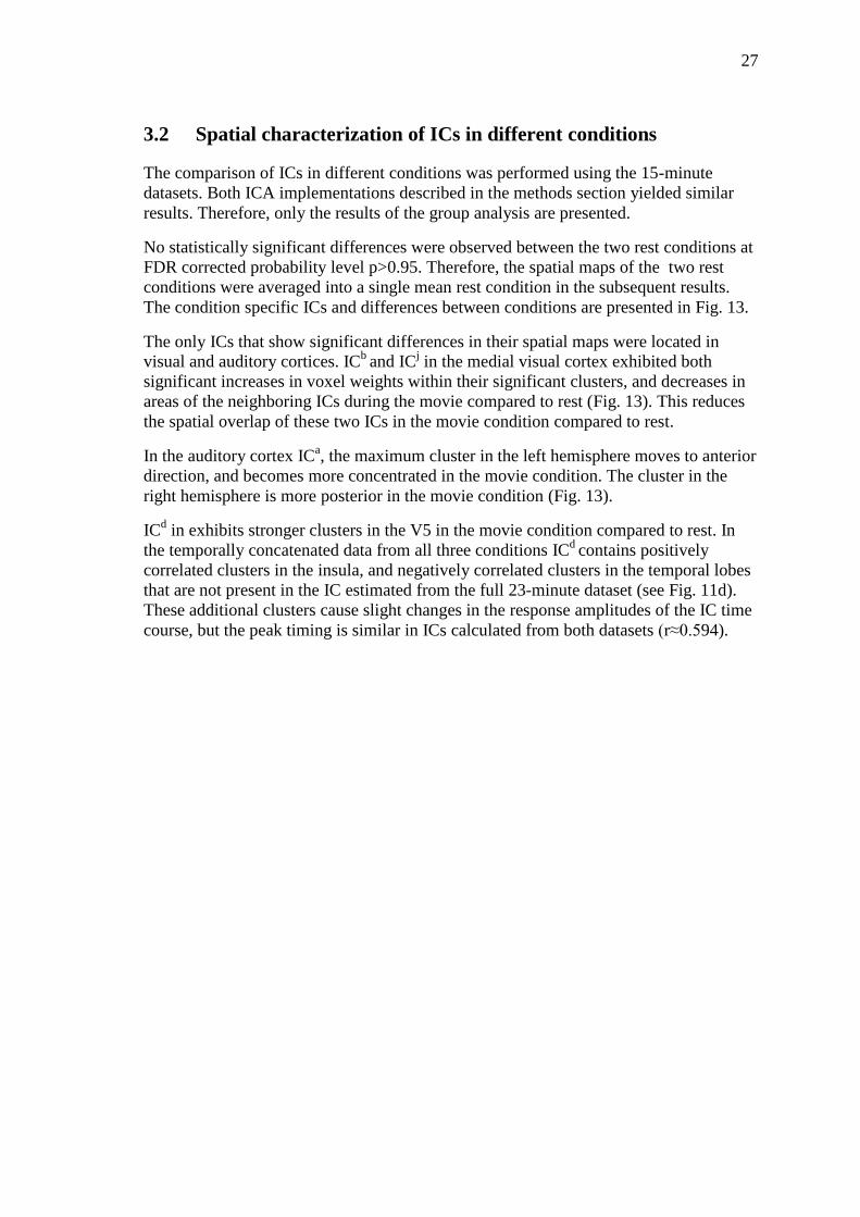
27

3.2 Spatial characterization of ICs in different conditions

The comparison of ICs in different conditions was performed using the 15-minute

datasets. Both ICA implementations described in the methods section yielded similar

results. Therefore, only the results of the group analysis are presented.

No statistically significant differences were observed between the two rest conditions at

FDR corrected probability level p>0.95. Therefore, the spatial maps of the two rest

conditions were averaged into a single mean rest condition in the subsequent results.

The condition specific ICs and differences between conditions are presented in Fig. 13.

The only ICs that show significant differences in their spatial maps were located in

visual and auditory cortices. ICb

and ICj in the medial visual cortex exhibited both

significant increases in voxel weights within their significant clusters, and decreases in

areas of the neighboring ICs during the movie compared to rest (Fig. 13). This reduces

the spatial overlap of these two ICs in the movie condition compared to rest.

In the auditory cortex ICa, the maximum cluster in the left hemisphere moves to anterior

direction, and becomes more concentrated in the movie condition. The cluster in the

right hemisphere is more posterior in the movie condition (Fig. 13).

ICd in exhibits stronger clusters in the V5 in the movie condition compared to rest. In

the temporally concatenated data from all three conditions ICd

contains positively

correlated clusters in the insula, and negatively correlated clusters in the temporal lobes

that are not present in the IC estimated from the full 23-minute dataset (see Fig. 11d).

These additional clusters cause slight changes in the response amplitudes of the IC time

course, but the peak timing is similar in ICs calculated from both datasets (r≈0.594).

28

Figure 13: Differences in spatial maps of four ICs. The component

images are presented in neurological convention and thresholded at

p>0.95, FDR corrected. Changes are thresholded by paired t-test of

condition specific spatial maps at p>0.95, FDR corrected. Five axial

slices best representing the changes in the component are presented.

3.3 Temporal structure of the independent components

Temporal structure of 16 of the 20 ICs described above (excluding ICs c, g, r, t) was

significantly similar in different subjects in the movie condition (one-tailed t-test for

positive correlation, p>0.999). These ICs were further separated into 28 ICs in the 141-

dimensional ICA (ICA141). None of the ICs showed synchronized activity between

subjects in the resting condition.

All ICs showing significantly similar temporal structure between subjects in the 141

dimensional ICA coincided with synchronized ICs in the 55dimensional ICA (ICA55),

and are presented in Appendix A.

29

ICs having significant temporal similarity between subjects in ICA141 are overlaid in

Fig. 14. These ICs cover bilaterally temporal, parietal and occipital brain areas, also

extending to the cerebellum. The ICs that were related to specific features of the movie

are described below.

Figure 14: All ICs showing significantly synchronized temporal structure

between subjects in ICA141. The color-coding corresponds to number of

overlapping ICs at each voxel.

3.3.1 Visual ICs

Nine of the sixteen ICs in ICA55 were located in the visual areas of the occipital cortex,

and the number was increased to twelve in ICA141.The temporal structure of these ICs

was compared to the annotated visual features.

The maximum clusters of ICd

overlap the middle temporal visual area (V5/MT). Area

V5 has been previously shown to be sensitive to motion in natural viewing condition

[49]. The timecourse of the ICd and the weighted sum of motion categories (see

methods) is presented in Fig. 15. Correlation coefficient of the two time courses is

0.587. Correlations were also calculated with the weighted sum of motions categories

for each voxel. Areas with significant correlation were largely overlapping with the

significant clusters of the ICd.

Weights for motion categories in the weighted sum were; 1 for hand motions, 0.4 for

mechanical motion, 0.2 for head, body and global motion, and 0 for inferred motion.

The correlation of ICd and inferred motion was negative, and correlation for mechanical

motion was positive but insignificant (p≈0.89). Other categories exhibited significant

(p>0.95) positive correlation with the time course of ICd.

30

Figure 15: Left: ICd overlapping the visual area V5, thresholded at

p>0.95, FDR corrected. Middle: Time course of the independent

component superimposed on the weighted sum of the motion categories..

Right: Correlation map depicting the voxels where activity correlated

signficicantly with the annotated visual features in 9/10 subjects,

thresholded at p>0.95, uncorrected.

Time course of the contrast-weighted edges was compared to each of the IC time

courses. Maximum correlation was 0.401 with the ICq, located in the occipital pole

coinciding with early visual areas (V1/V2). Spatial map and time course of ICq and the

time course of edges in the movie are presented in Fig. 16. Correlation of presence of

edges and time-course of two other visual-cortex ICs (ICm

and ICo) was also significant

(p>0.9999, correlation coefficients 0.281 and 0.308, respectively). No significant

correlations with single voxels were observed.

Figure 16: Left: Spatial map of visual ICq, thresholded at p>0.95, FDR

corrected. Right: Time courses of the visual IC and the contrast

weighted sum of edges in the video.

3.3.2 Auditory ICs

In ICA55, ICa located in the superior temporal gyrus and dorsal parts of the superior

temporal sulcus (STS) was found to follow features of the sound track. However, as is

shown in Fig. 17, high activation peaks to speech and singing were observed

independent of loudness. In all cases where voice is present, the peaks are notably

higher than in the time course obtained by convoluting the loudness envelope of the

audio track with a canonical HRF.

31

Figure 17: Left: Spatial location of the auditory-cortex ICa. Top right:

Timecourse of the IC and audio envelope convoluted with the canonical

HRF. Arrows indicate the onset of each occurrence of voice. Bottom

right: Annotations showing time intervals when voice (speech and

singing) or music was present in the audio track of the movie.

The sensitivity of the auditory ICa to auditory features was further studied by calculating

correlations between the BOLD signal strength in all brain voxels and the loudness

envelope of the sound track and occurrence of speech in the sound track (Fig. 18).

The loudness envelope correlated with activity in a relatively small area, coinciding

with location of Heschl’s gyrus (for anatomical localization see Fig. 19). Primary

auditory cortex in generally thought to be located in the mesial part of the anterior

Heschl’s gyrus [62]. A small correlated area was also observed in the right V5 visual

area (MNI152 coordinates 42, -66, -8). Occurrences of speech correlated with activity in

the superior temporal sulcus (STS) bilaterally and posterior middle temporal gyrus

(MTG) of the left hemisphere in addition to the areas correlated with the loudness

envelope (Fig. 18). The areas within STS are consistent with voice sensitive regions

reported earlier [63].

Figure 18: Auditory-cortex IC is shown in blue. Cortical area where

voxels correlated with occurrence of voice are indicate by red. Yellow

indicates the voxels whose activity correlated with loudness of the audio

track. Areas are thresholded at p>0.95, uncorrected.

The locations, which correlated with the audio loudness for individual subjects are

presented in Fig. 19. Extensive areas of the brain are correlated with the loudness

32

envelope at significance level p>0.95 despite the FDR correction. Therefore, the

maximum correlation coefficient, and its location are indicated for each subject. The

threshold level for the correlation coefficient is proportional to the maximum correlation

of each subject to make the areas of maximum correlation visible in the figure. For eight

of the ten subjects, the location of the maximum correlation is in the mesial part of the

anterior Heschl’s gyrus, however significant correlation is also seen in the surrounding

areas. The maximally correlated voxel for subject 9 is located in white matter. The only

significantly correlated area for subject 10 is located in the right superior frontal gyrus.

1. Max 0.25

Thr 0.19

2. Max 0.31

Thr 0.23

3. Max 0.35

Thr 0.26

4. Max 0.29

Thr 0.22

5. Max 0.35

Thr 0.26

6. Max 0.22

Thr 0.17

7. Max 0.39

Thr 0.29

8. Max 0.40

Thr 0.30

9. Max 0.33

Thr 0.25

10. Max 0.19

Thr 0.14

Correlation probability,

p > 0.95, FDR corrected

Area of maximum correlation, Max ≥ r > Thr

Figure 19: Loudness correlated areas for nine subjects. Blue indicates

areas where correlation was significant at p>0.95, FDR corrected. Red

indicates the location of maximum correlation coefficient (r). Max

indicates the maximum correlation coefficient for the subject and Thr

indicates the threshold level of the red area (0.75*Max). Images are

presented in neurological convention. For anatomical localization, the

correlated areas are presented on each subjects own T1 image registered

to MNI152 standard.

33

The auditory ICa is included in IC

l, which covers area related to language processing in

temporal lobe and posterior division of inferior frontal gyrus (IFG) in the left

hemisphere [63]. ICA141 separates ICl into two separate ICs shown in Fig. 20 (A10 and

A28 in Appendix A). However, the area in the inferior frontal gyrus is not seen in these

ICs. The area correlated with voice (green in Fig. 20) in the left hemisphere is located in

the intersection of the strongest clusters of these two ICs. In the right hemisphere the

speech correlated area is located between the ICs. ICA28

is located in the medial STS,

STG and MTG. Its activation is consistently related to speech, but not to singing. ICA10

is located in the posterior temporal lobe and anterior STG. It exhibits similar sensitivity

to speech as ICA28

, but also activates during the occurrence of singing. The posterior

temporal area of the ICA10

coincides with Brodmann area 22, often referred to as

Wernicke’s speech area [64].

Figure 20: Left: Two language related ICs, a) ICA28

and b) ICA10

located

mainly in the left temporal lobe. Voxels whose activity correlated with

speech and singing, but not the loudness of the entire sound track, are

indicated in green. Right: Time courses of the ICs ± standard deviation.

Bottom: Annotations showing time intervals when there was speech,

singing or instrumental music in the movie sound track.

34

3.3.3 Parietal ICs

Three separate ICs (ICf, IC

i and IC

n in Figs. 11 and 12) covered large areas of the

superior and inferior parietal lobules. They contained additional clusters in V5, superior

precentral gyrus, and posterior inferior frontal gyrus. All three ICs seem to be active

especially during movie scenes including hand actions, for example writing and opening

or closing envelopes.

In ICA141 the three parietal ICs were further separated into 5 ICs (A1, A4, A9, A20

and A24 in Appendix A), which are presented in Fig. 21 including scenes associated

with peak activity. ICA1

and ICA4

reside in analogous areas of superior parietal lobule

(SPL) and lateral occipital lobe. Both components also include parts of precentral gyrus.

ICA1

additionally includes areas of the cerebellum, and ICA4

includes part of V5. ICA24

and ICA9

reside in analogous areas within inferior parietal lobule (IPL), V5/MT, and

inferior frontal gyrus. ICA20

is located in the intra-parietal sulcus (IPS) and adjacent

areas of the SPL and IPL. The activation peaks of all five ICs coincide with occurrences

of hand actions. However, some scenes of hand actions do not elicit activity in all ICs

(see scenes A-D in Fig. 21).

Correlation analysis was performed for the annotated time course of hand motions to

further investigate the specific relation of hand actions and the parietal ICs. The

significantly correlated areas coincide with the bilateral IPS, left-hemisphere dominant

V5, superior part of the precentral gyrus, and small areas of the right inferior parietal

lobule (Fig. 22).

35

Figure 21: Left: Five ICs located mainly in the parietal lobe. Right: Time

courses of independent components ± standard deviation. Bottom:

Examples of scenes associated with peak activity.

Figure 22: Cortical area where voxels correlated with occurrence of hand

motion in the movie. The color-coding corresponds to group probability

of correlation, calculated using Fisher’s method (u=9, n=10, see

methods). The image is thresholded at p>0.95.

36

4 Discussion

Independent component analysis revealed 18 ―resting state networks‖ present both

during rest and movie conditions. The ICs were notably similar in all three conditions.

Only differences in the spatial organization of the ICs were observed in the visual and

auditory cortices, where four ICs were concentrated to smaller regions in the movie

condition than in the rest condition. Two additional ICs were found in the visual cortex

in the movie condition in the 23-minute data. Sixteen of the ICs activated similarly

between subjects during the movie condition, and were divided further into 28 ICs by

increasing the dimensionality of ICA. The ICs showing similar activity patterns

between subjects were located in sensory and associative areas in temporal, occipital

and parietal lobes. Several ICs coincided with location of voxels that correlated with

features annotated from the movie, such as visual motion, sum of contrast edges in the

visual field, auditory features and hand actions. Correlation analysis also divided the

auditory ICa into voice and loudness sensitive areas.

The RSNs found in the current study fit well with areas reported in prior research [6; 7],

with some notable exceptions. Some networks typically reported as single ICs were split

into multiple ICs, and unlike in many resting state studies, no consistent networks were

specific to only the prefrontal cortex (PFC). Some ICs did however include clusters in

the PFC (e.g. ICi, IC

k and IC

l). In fact, ICA did separate multiple networks in the PFC,

but they appeared artifactual in nature, their signal powers were not concentrated in the

frequency range of interest, or they were not always reproducible on separate run of the

ICA algorithm. Additionally none of the ICs located in the PFC exhibited significant

synchrony between subjects during the movie. This may be due to strict demands set by

the statistical testing, but there is evidence that not all movies are successful at eliciting

reliable responses in the PFC [4].

The ICp, which includes areas typically associated with the default mode network

included a very small area in the frontal pole in the current study. The DMN is often

reported to include extensive areas of ventromedial, and dorsomedial prefrontal cortex.

However, the extent of this node of the network appears to change from one study to the

next [2; 6; 44], but it is unclear if this is due to the employed methods, inter-subject

variability, or combination of both.

Significant differences between the two resting state conditions were not found. This is

consistent with a recent report of remarkable stability and replicability of the brain

organization at rest [7]. Prolonged changes have been previously reported following

stimulation [11], but no such observations were made in the current analyses. However,

the ICs were calculated over the whole 15-minute resting sessions, which may hide

short changes immediately after the movie. It may be useful to study the data over

shorter time windows in the future.

Parts of the visual and auditory cortices were the only areas showing consistent changes

when directly comparing ICs of movie and rest conditions using 15-minute datasets.

These areas exhibited clusters, which were more specific in the movie condition

compared to rest, showing tighter maxima in the clusters and decreased voxel weights

37

around the significant areas of the IC. However, the spatial organization of the networks

in general was almost identical in all three conditions, supporting the idea, that RSNs

may reveal the underlying functional organization of the brain [6].

Most studies so far have concentrated on either the resting state networks or finding

neural correlates of external stimulation. However, the current study demonstrates that

many of the RSNs activate similarly across subjects during natural stimulation, and their

time courses are correlated with features of the stimulus. This suggests that the

activation patterns of the RSNs during complex stimulation may help reveal the

functional significance of these networks. However, the movie used in the current study

elicited correlated activity mainly in the posterior regions of the cerebral cortex.

Therefore, further research is needed to examine the functional specialization of other

RSNs.

The IC in the V5 was sensitive to all motion categories apart from the inferred motion,

which did not elicit correlated activation in the V5. While the correlation of mechanical

motion with V5 activity was insignificant, mechanical motion received the second

highest weight in the motion sum. This appears to be due to the structure of the movie.

Mechanical motion was present in relatively few time intervals, and other motion

categories were typically not seen simultaneously in the image. Therefore, the overall

correlation was small, but the contribution to the time course of overall motion was

significant. Earlier research [50] revealed areas consistent with the V5 IC to be

responsible for coding local, but not global motion, which was proposed to be processed

in the posterior parietal lobe. However, the current study did not reveal any separate

areas correlated with the global motion category.

Activation time courses of both visual ICs (Figs. 15 and 16) are significantly correlated

with individual stimulus features but the annotations clearly explain only part of the

activation changes. The activation strengths differ from the annotation time courses and

there are timeframes in both of the examples during which the time courses are

uncorrelated. Additionally, no voxels were found to correlate with the sum of edges.

However, because different parts of the visual field are mapped to different locations on

the cortex [64] finding a single voxel that correlated with all the edges in the visual field

was unlikely. The time course of edges was calculated to approximate the sum of

activation of all the simple cells in the visual cortex, which have receptive fields similar

to the Gabor filters used in the filter bank. Because ICs represent weighted sums of

individual voxel time courses, they were assumed to better fit the time course

representing the sum signal.

The simple sum of edges in the movie is certainly an oversimplification of the

activation in the visual cortex. For example, different weights should be assigned to the

edges depending on the direction that the subject is looking because of the

magnification of the fovea in the visual cortex in comparison to the peripheral visual

field [65]. However, the sum was calculated to demonstrate the feasibility of mapping

edges in the images to locations in the visual cortex during complex visual stimulation.

Retinotopic mapping of the visual cortex has been studied in the past using simple

visual stimuli [64]. If similar mapping of visual edges in the movie to locations on the

visual cortex could be achieved, it would allow the inference of gaze direction without

38

the need to record the subjects’ eye motions. However, this will be studied further in

future research, when eye motion data is available to verify the results.

The auditory cortex was divided into loudness and voice sensitive areas. For one subject

the maximum correlation with audio loudness was located in white matter, which may

have been caused by registration error, as the overall shape of the correlated area was

consistent with those observed in other subjects. No regions of the temporal lobes of

one subject correlated with the loudness envelope, possibly due to individual

differences in the delay of the hemodynamic response.

The division of auditory areas fit well with prior reports [66]. These findings were

initially based only on observed activation patterns. The results suggest that careful

analysis of IC time courses can be used to reveal features of the organization of the

cerebral cortex in the absence of prior knowledge of the regional specialization. In

addition to the auditory cortex, a small area consistent with the location of the inferior

parts of the V5 in the right hemisphere correlated with the auditory stimulus. V5 is

typically associated with processing of visual motion. However, V5 in the right

hemisphere has also been reported to exhibit activation to auditory motion in the

absence of visual stimulation [67]. This is consistent with the location correlated with

audio in the current study.

The loudness envelope of the audio track and visual motion were found to be

significantly correlated in the movie. However, the area correlated with audio loudness

did not overlap the area correlated with visual motion. Nevertheless, this highlights the

need for careful analysis of the stimulus as well as the BOLD signal before making

conclusions in naturalistic settings, because there are several features in the stimulus

which could be responsible for the activation in the brain.

The subdivisions found in the auditory cortex suggested, that other ICs may also contain

multiple areas specializing in more specific features of the stimulus. This was studied

by increasing the dimensionality of ICA. The dimensionality estimates for the 23-

minute datasets recorded in the movie condition were almost three times higher than the

estimate for the temporally concatenated data of all subjects and conditions using the15-

minute datasets. Increasing the dimensionality of the ICA subdivided the ICs into

smaller functional units in the movie condition.

The number of temporally coherent ICs doubled when the dimensionality was

increased, but critically, the collective area of these ICs remained unchanged regardless

of the dimensionality. This demonstrates that IC selection through the temporal

correlation of the subjects’ ICs is a robust method for selecting meaningful ICs for

temporal analysis during movie viewing regardless of the dimensionality. Intuitively,

this temporal synchronization is in fact a requirement for any inference to be made on

the group level. If the ICs do not act similarly between subjects, any peaks in the mean

time course may be coincidental.

The 141 dimensional analysis divided the left temporal lobe into two highly overlapping

ICs. Most notably, it appears that specific areas present in ICA10

(see Fig. 20b) are

sensitive to singing as well as speech, while ICA28

(Fig. 20a) does not exhibit activity

39

when singing is present. This suggests that singing is interpreted partially through

different mechanisms than speech, and some areas specifically sensitive to singing may

be found in the area of ICA28

not overlapping ICA10

. This observation should be studied

more thoroughly in future research, because the movie used in the current study

contained only one occurrence of singing. Some evidence has been reported on different

neural substrates responsible for processing speech and singing [68]. For example, the

location of the anterior temporal sub-cluster of ICA28

was reported to be more sensitive

to singing than to speech, but no reports have been published where such differentiation

has been achieved using data driven methods during complex stimulation.

Five ICs located primarily in the parietal cortex were found, which were activated

during hand actions. Watching manual manipulations has been previously [69]

associated with activity in the IPS which separates the superior and inferior parietal

lobules and coincides with parts of all five ICs, as well as the area discovered by

correlation analysis. Others [70; 71] have associated the areas of these ICs to the so-

called dorsal attention network proposed to be responsible for the top-down

mechanisms for reorienting attention. The dorsal attention network has been reported

[72] to show hemispheric preference to stimuli in the opposite half of the visual field.

Intriguingly this network was consistently separated into highly lateralized components

allowing direct comparison of activation strengths between the two hemispheres.

Differences were observed in response amplitudes of the five ICs. However, the

subjects’ gaze directions were not recorded in the current study making it uncertain

which visual features the subjects were looking at. Therefore, the proposed hemispheric

preference and other possible causes for the differential response amplitudes will be

studied further in the future when subjects’ eye motion data is recorded.

The annotations done in the current study were of low resolution. Significantly higher

precision could have been achieved especially for the sound track. However, because of

the temporal smoothing introduced by the HRF and the low temporal resolution of the

fMRI data, the one-second resolution was considered adequate. For validation of the

assumption, the RMS sound envelope was calculated using 1/50 second resolution, but

the changes were very small in the signal convoluted with HRF after down sampling.

Some short peaks were more pronounced in the higher resolution signal, but the

correlated areas remained unchanged despite the enhanced precision of the RMS

envelope.

4.1 Conclusions

The results of the current study suggest that both model based and model free methods

can be used to reveal similar patterns of brain activation. However, creating models of a

complex stimulus is time consuming and difficult. Therefore, data driven analysis

methods are a useful complement for model based methods. They may be used as a

guide for selecting relevant features to model when the comprehensive modeling of all

stimulus features is not feasible. In addition, model free methods are essential when the

underlying brain activation cannot be predicted accurately [6] such as in resting state

condition for example.

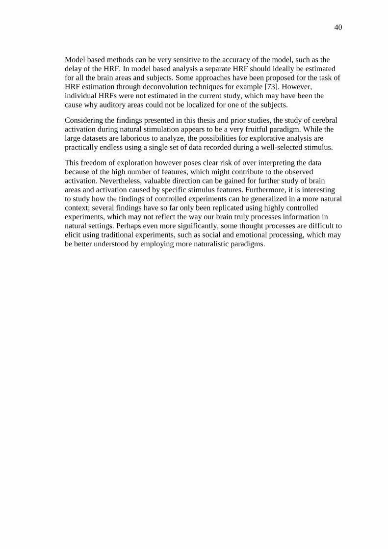
40

Model based methods can be very sensitive to the accuracy of the model, such as the

delay of the HRF. In model based analysis a separate HRF should ideally be estimated

for all the brain areas and subjects. Some approaches have been proposed for the task of

HRF estimation through deconvolution techniques for example [73]. However,

individual HRFs were not estimated in the current study, which may have been the

cause why auditory areas could not be localized for one of the subjects.

Considering the findings presented in this thesis and prior studies, the study of cerebral

activation during natural stimulation appears to be a very fruitful paradigm. While the

large datasets are laborious to analyze, the possibilities for explorative analysis are

practically endless using a single set of data recorded during a well-selected stimulus.

This freedom of exploration however poses clear risk of over interpreting the data

because of the high number of features, which might contribute to the observed

activation. Nevertheless, valuable direction can be gained for further study of brain

areas and activation caused by specific stimulus features. Furthermore, it is interesting

to study how the findings of controlled experiments can be generalized in a more natural

context; several findings have so far only been replicated using highly controlled

experiments, which may not reflect the way our brain truly processes information in

natural settings. Perhaps even more significantly, some thought processes are difficult to

elicit using traditional experiments, such as social and emotional processing, which may

be better understood by employing more naturalistic paradigms.

41

5 Bibliography

[1]. Friston, K. Causal Modelling and Brain Connectivity in Functional Magnetic

Resonance Imaging. PLoS Biology. 2009, Vol. 7, 2.

[2]. Damoiseaux, J. S., et al. Consistent resting-state networks across healthy subjects.

PNAS. 2006, Vol. 103, 37, pp. 13848-13853.

[3]. Jääskeläinen, Iiro P., et al. Inter-Subject Synchronization of Prefrontal Cortex

Hemodynamic Activity During Natural Viewing. Open Neuroimaging. 2008, Vol. 2.

[4]. Hasson, Uri, Malach, Rafael and Heeger, David J. Reliability of cortical activity

during natural stimulation. Trends in Cognitive Sciences. 2009, Vol. 14, 1, pp. 40-48.

[5]. Bartels, Andreas and Zeki, Semir. The chronoarchitecture of the human brain—

natural viewing conditions reveal a time-based anatomy of the brain. NeuroImage.

2004, Vol. 22, 1, pp. 419-433.

[6]. Beckmann, Christian F., et al. Investigations into resting-state connectivity using

independent component analysis. Philosophical Transactions of Royal Society B. 2005,

Vol. 360, 1457, pp. 1001–1013.

[7]. Biswal, Bharat B., et al. Toward discovery science of human brain function.

PNAS. 2010, Vol. 107, 10, pp. 4734-4739.

[8]. Fransson, P. and Marrelec, G. The precuneus/posterior cingulate cortex plays a

pivotal role in the default mode network: Evidence from a partial correlation network

analysis. NeuroImage. 2008, Vol. 42, 3, pp. 1178-84.

[9]. Iacoboni, Marco, et al. Watching social interactions produces dorsomedial

prefrontal and medial parietal BOLD fMRI signal increases compared to a resting

baseline. NeuroImage. 2004, Vol. 21, 3, pp. 1167-1173.

[10]. Harrison, Ben J., et al. Consistency and functional specialization in the default

mode brain network. PNAS. 2008, Vol. 105, 28, pp. 9781–9786.

[11]. Hasson, Uri, Nusbaum, Howard C. and Small, Steven L. Task-dependent

organization of brain regions active at rest. PNAS. 2009, Vol. 106, 26, pp. 10841-10846.

[12]. Waites, Anthony B., et al. Effect of prior cognitive state on resting state networks

measured with functional connectivity. Human Brain Mapping. 2004, Vol. 24, 1, pp.

59-68.

[13]. Ogawa, Seiji, et al. Oxygenation-sensitive contrast in magnetic resonance image

of rodent brain at high magnetic fields. Magnetic Resonance in Medicine. 1988, Vol.

14, 1, pp. 68-78.

[14]. Mandeville, Joseph B. and Rosen, Bruce R. Functional MRI. [book auth.]

Arthur W. Toga and John C. Mazziotta. Brain Mapping: The Methods, 2nd edition. San

Diego, California : Elsevier Science, 2002, pp. 315-349.

42

[15]. Glover, Paul and Bowtell, Richard. Medical imaging: MRI rides the wave.

Nature. 2009, Vol. 457, 7232, pp. 971-972.

[16]. Webb, Andrew G. Introduction to Biomedical Imaging. Hoboken, New Jersey :

Wiley-IEEE press, 2003.

[17]. Huettel, Scott A., Song, Allen W. and McCarthy, Gregory. Functional

Magnetic Resonance Imaging. Sunderland, Massachusetts : Sinauer Associates, Inc,

2004.

[18]. Deshmukh, Ajay V. and Gadre, Vikram M. Functional Magnetic Resonance

Imaging: Novel Transform Methods. New Delhi : Narosa Publishing House Pvt. Ltd.,

2008.

[19]. Jackson, Graeme D., Kuzniecky, Ruben I. and Pell, Gaby S. Principles of

Magnetic Resonance Imaging. [book auth.] Ruben I. Kuzniecky and Graeme D.

Jackson. Magnetic Resonance in Epilepsy, 2nd edition. San Diego, California : Elsevier

Inc, 2005.

[20]. Logothetis, N. K. and Wandell, B.A. Interpreting the BOLD signal. Annual

review of physiology. 2004, Vol. 66, pp. 735-769.

[21]. Afonso, David M., Sanches, João M. and Lauterbach, Martin H. Neural

physiological modeling towards a hemodynamic response function for fMRI.

Proceedings of the 29th Annual International Conference of the IEEE EMBS, 22-26.8.

2007, Cité Internationale, Lyon, France. 2007, pp. 1615-1618.

[22]. Tohka, Jussi, et al. Automatic independent component labeling for artifact

removal in fMRI. NeuroImage. 2008, Vol. 39, 3, pp. 1227-1245.

[23]. Rad, Gholamali Rezai and Larijani, Houtan Haddad. A Comparative Study of

ICA Based Approaches for Separation of Components in Functional MRI Sequences.

3rd International Conference on Geometric Modeling and Imaging, 9-11.7.2008,

London, UK. 2008, pp. 87-91.

[24]. David, Olivier, et al. Identifying Neural Drivers with Functional MRI: An

Electrophysiological Validation. PLoS Biology. 2008, Vol. 6, 12, pp. 2684-2697.

[25]. Duann, Jeng-Ren, et al. Single-Trial Variability in Event-Related BOLD Signals.

NeuroImage. 2002, Vol. 15, 4, pp. 823–835.

[26]. Hyvärinen, Aapo and Oja, Erkki. Independent Component Analysis: Algorithms

and Applications. Neural Networks. 2000, Vol. 13, 4-5, pp. 411-430.

[27]. Correa, Nicolle, Adali, Tülay and Calhoun, Vince D. Performance of Blind

Source Separation Algorithms for FMRI Analysis using a Group ICA Method.

Magnetic Resonance Imaging. 2007, Vol. 25, 5, pp. 684-694.

43

[28]. Calhoun, V. D., et al. Spatial and Temporal Independent Component Analysis of

Functional MRI Data Containing a Pair of Task-Related Waveforms. Human Brain

Mapping. 2001, Vol. 13, 1, pp. 43-53.

[29]. Beckmann, C. F. and Smith, S. M. Tensorial extensions of independent

component analysis for multisubject FMRI analysis. NeuroImage. 2005, Vol. 25, 1, pp.

294-311.

[30]. Särelä, Jaakko and Vigário, Ricardo. The Problem of Overlearning in High-

Order ICA Approaches: Analysis and Solutions. [ed.] J. Mira and A. Prieto.

Proceedings of the 6th international Work-Conference on Artificial and Natural Neural

Networks: Bio-inspired Applications of Connectionism-Part II, 13-16.6.2001. Lecture

Notes in Computer Science. : Springer-Verlag, London, 2001, Vol. 2085, pp. 818-825.

[31]. Wall, Michael E., Rechtsteiner, Andreas and Rocha, Luis M. Singular value

decomposition and principal component analysis. [ed.] D.P. Berrar, W. Dubitzky and

M. Granzow. A Practical Approach to Microarray Data Analysis. Norwell : Kluwer,

2003, pp. 91-109.

[32]. Li, Yi-Ou, Adali, Tülay and Calhoun, Vince D. Estimating the Number of

Independent Components for Functional Magnetic Resonance Imaging Data. Human

Brain Mapping. 2007, Vol. 28, 11, pp. 1251–1266.

[33]. Cordes, Dietmar and Nandy, Rajesh R. Estimation of the intrinsic

dimensionality of fMRI data. NeuroImage. 2006, Vol. 29, 1, pp. 145-154.

[34]. Bartels, Andreas and Zeki, Semir. Brain dynamics during natural viewing

conditions—A new guide for mapping connectivity in vivo. NeuroImage. 2005, Vol.

24, 2, pp. 339-349.

[35]. Hasson, Uri, et al. Intersubject Synchronization of Cortical Activity During

Natural Vision. Science. 2004, Vol. 303, 5664, pp. 1634-1640.

[36]. van den Heuvel, Martijn, Mandl, Rene and Hulshoff Pol, Hilleke. Normalized

Cut Group Clustering of Resting-State fMRI Data. PLoS One. 2008, Vol. 3, 4. e2001.

doi:10.1371/journal.pone.0002001.

[37]. Birn, Rasmus M, Murphy, Kevin and Bandettini, Peter A. The Effect of

Respiration Variations on Independent Component Analysis Results of Resting State

Functional Connectivity. Human Brain Mapping. 2008, Vol. 29, 7, pp. 740-750.

[38]. Birn, Rasmus M., et al. Separating respiratory-variation-related fluctuations from

neuronal-activity-related fluctuations in fMRI. NeuroImage. 2006, Vol. 31, 4, pp. 1536-

1548.

[39]. Xiaoping, Xie, Zhitong, Cao and Xuchu, Weng. Spatiotemporal nonlinearity in

resting-state fMRI of the human brain. NeuroImage. 2008, Vol. 40, 4, pp. 1672-1685.

44

[40]. Biswal, Bharat, et al. Functional connectivity in the motor cortex of resting

human brain using echo-planar mri. Magnetic Resonance in Medicine. 1995, Vol. 34, 4,

pp. 537 - 541.

[41]. Thirion, Bertrand, Dodel, Silke and Poline, Jean-Baptiste. Detection of signal

synchronizations in resting-state fMRI datasets. NeuroImage. 2006, Vol. 29, 1, pp. 321-

327.

[42]. Zuendorf, Gerhard, et al. Efficient principal component analysis for multivariate

3D voxel-based mapping of brain functional imaging data sets as applied to FDG-PET

and normal aging. NeuroImage. 2002, Vol. 18, 1, pp. 13-21.

[43]. Beckmann, C. F. and Smith, S. M. Probabilistic independent component analysis

for functional magnetic resonance imaging. IEEE Transactions on Medical Imaging.

2004, Vol. 23, 2, pp. 137-152.

[44]. Long, Xiang-Yu, et al. Default mode network as revealed with multiple methods

for resting-state functional MRI analysis. Journal of neuroscience methods. 2008, Vol.

171, 2, pp. 349-355.

[45]. Hasson, Uri, Nusbaum, Howard C. and Small, Steven L. Brain Networks

Subserving the Extraction of Sentence Information and Its Encoding to Memory.

Cerebral cortex. 2007, Vol. 17, 12, pp. 2899-2913.

[46]. Boly, M., et al. Intrinsic Brain Activity in Altered States Intrinsic Brain Activity

in Altered States: How Conscious Is the Default Mode of Brain Function? Annals of the

New York Academy of Sciences. 2008, Vol. 1129, pp. 119–129.

[47]. Malinen, Sanna, Hlushchuk, Yevhen and Hari, Riitta. Towards natural

stimulation in fMRI—Issues of data analysis. NeuroImage. 2007, Vol. 35, 1, pp. 131-

139.

[48]. Calhoun, Vince D., et al. Different Activation Dynamics in Multiple Neural

Systems During Simulated Driving. Human Brain Mapping. 2002, Vol. 16, 3, pp. 158-

167.

[49]. Hejnar, Martin P., Kiehl, Kent A. and Calhoun, Vince D. Interparticipant

correlations: A model free FMRI analysis technique. Human Brain Mapping. 2007, Vol.

28, 9, pp. 860-867.

[50]. Bartels, A., Zeki, S. and Logothetis, N. K. Natural Vision Reveals Regional

Specialization to Local Motion and to Contrast-Invariant, Global Flow in the Human

Brain. Cerebral Cortex. 2008, Vol. 18, 3, pp. 705-717.

[51]. Hasson, Uri, et al. Neurocinematics: The Neuroscience of Film. Projections.

2008, Vol. 2, 1, pp. 1-26.

[52]. Smith, S. M., et al. Advances in functional and structural MR image analysis and

implementation as FSL. NeuroImage. 2004, Vol. 23, Supplement 1, pp. S208-S219.

45

[53]. Woolrich, M. W., et al. Bayesian analysis of neuroimaging data in FSL.

NeuroImage. 2009, Vol. 45, 1, Supplement 1, pp. S173-S186.

[54]. Smith, S. Fast Robust Automated Brain Extraction. Human Brain Mapping. 2002,

Vol. 17, 3, pp. 143-155.

[55]. Himberg, J., Hyvärinen, A. and Esposito, F. Validating the independent

components of neuroimaging time-series via clustering and visualization. NeuroImage.

2004, Vol. 22, 3, pp. 1214-1222.

[56]. Jenkinson, M., et al. Improved optimisation for the robust and accurate linear

registration and motion correction of brain images. NeuroImage. 2002, Vol. 17, 2, pp.

825-841.

[57]. Ringach, Dario L. Mapping receptive fields in primary visual cortex. The Journal

of Physiology. 2004, Vol. 558, 3, pp. 717-728.

[58]. Benjamini, Yoav and Yekutieli, Daniel. The control of the false discovery rate in

multiple testing under dependency. The Annals of Statistics. 2001, Vol. 29, 4, pp. 1165-

1188.

[59]. Himberg, Johan and Hyvärinen, Aapo. Icasso: software for investigating the

reliability of ICA estimates by clustering and visualization. In Proc. 2003 IEEE

Workshop on Neural Networks for Signal Processing (NNSP2003). Toulouse, France :

s.n., 2003, pp. 259-268.

[60]. Heller, Ruth, et al. Conjunction group analysis: An alternative to mixed/random

effect analysis. NeuroImage. 2007, Vol. 37, 4, pp. 1178-1185.

[61]. Zou, Qi-Hong, et al. An improved approach to detection of amplitude of low-

frequency fluctuation. Journal of Neuroscience Methods. 2008, Vol. 172, 1, pp. 137-

141.

[62]. Warrier, Catherine, et al. Relating Structure to Function: Heschl’s Gyrus and

Acoustic Processing. The Journal of Neuroscience. 2009, Vol. 29, 1, pp. 61-69.

[63]. Gazzaniga, Michael S., Ivry, Richard B. and Mangun, George R. Cognitive

Neuroscience: The Biology Of The Mind. 2nd Edition. New York : W.W. Norton &

Company, Inc., 2002.

[64]. Engel, Stephen A., Glove, Gary H. and Wandell, Brian A. Retinotopic

Organization in Human Visual Cortex and the Spatial Precision of Functional MRI.

Cerebral Cortex. 1997, Vol. 7, 2, pp. 181-192.

[65]. Schira, Mark M., et al. The Foveal Confluence in Human Visual Cortex. The

Journal of Neuroscience. 2009, Vol. 29, 28, pp. 9050-9058.

[66]. Belin, Pascal, et al. Voice-selective areas in human auditory cortex. Nature. 2000,

Vol. 403, 6767, pp. 309-312.

46

[67]. Poirier, Colline, et al. Specific activation of the V5 brain area by auditory motion

processing: An fMRI study. Cognitive Brain Research. 2005, Vol. 25, 3, pp. 650-658.

[68]. Callan, Daniel E., et al. Song and speech: Brain regions involved with perception

and covert production. NeuroImage. 2006, Vol. 31, 3, pp. 1327-1342.

[69]. Daw, Nathaniel D., et al. Cortical substrates for exploratory decisions in humans.

Nature. 2006, Vol. 441, 7095, pp. 876-879.

[70]. Salmi, Juha, et al. Brain networks of bottom-up triggered and top-down

controlled shifting of auditory attention. Brain Research. 2009, Vol. 1286, pp. 155-164.

[71]. Corbetta, Maurizio, Patel, Gaurav and Shulman, Gordon L. The Reorienting

System of the Human Brain: From Environment to Theory of Mind. Neuron. 2008, Vol.

58, 3, pp. 306-324.

[72]. Serences, John T. and Yantis, Steven. Spatially Selective Representations of

Voluntary and Stimulus-Driven Attentional Priority in Human Occipital, Parietal, and

Frontal Cortex. Cerebral Cortex. 2007, Vol. 17, 2, pp. 284-293.

[73]. Lu, Yingli, et al. Using voxel-specific hemodynamic response function in EEG-

fMRI data analysis. NeuroImage. 2006, Vol. 32, 1.

47

Appendix A

This appendix shows the areas and time courses of all independent components whose

median pairwise correlation between subjects was significant (p>0.9999). Spatial maps

are thresholded at p>0.95, FDR corrected, and are presented in neurological convention

on an MNI152 standard brain template. Slices go through the maximum voxel of the IC.

Slice coordinates are indicated in MNI152 standard space. Time series plots show the

standardized mean time course. The highlighted area corresponds to mean time course

±1 standard deviation.

48

49

50

51