Functional linear regression with functional response�

David Benatia

Université de Montréal

Marine Carrasco

Université de Montréal

Jean-Pierre Florens

Toulouse School of Economics

February 2015

Abstract

In this paper, we develop new estimation results for functional regressions

where both the regressor Z(t) and the response Y (t) are functions of an index

such as the time or a spatial location. Both Z(t) and Y (t) are assumed to belong

to Hilbert spaces. The model can be thought as a generalization of the standard

regression where the regression coe¢ cient is now an unknown operator �. An

interesting feature of our model is that Y (t) depends not only on contemporaneous

Z(t) but also on past and future values of Z.

We propose to estimate the operator � by Tikhonov regularization, which

amounts to apply a penalty on the L2 norm of �. We derive the rate of convergence

of the mean-square error, the asymptotic distribution of the estimator, and develop

tests on �. Often, the full trajectories are not observed but only a discretized

version is available. We address this issue in the scenario where the data become

more and more frequent (in-�ll asymptotics). We also consider the case where Z

is endogenous and instrumental variables are used to estimate �.

KeyWords: Functional regression, instrumental variables, linear operator,Tikhonov

regularization

�The authors thank the participants of the 6th French Econometrics Conférence and especially theirdiscussant Jan Johannes for helpful comments.

1 Introduction

With the increase of storage capability, continuous time data are available in many

�elds including �nance, medecine, meteorology, and microeconometrics. Researchers,

companies, and governments look for ways to exploit this rich information. In this

paper, we develop new estimation results for functional regressions where both the

regressor Z(t) and the response Y (t) are functions of an index such as the time or

a spatial location. Both Z(t) and Y (t) are assumed to belong to Hilbert spaces. The

model can be thought as a generalization of the standard regression where the regression

coe¢ cient is now an unknown operator �. An interesting feature of our model is that

Y (t) depends not only on contemporaneous Z (t) but also on past and future values of

Z.

We propose to estimate the operator � by Tikhonov regularization, which amounts

to apply a penalty on the L2 norm of �. The choice of a L2 penalty, instead of L1 used

in Lasso, is motivated by the fact that - in the applications we have in mind - there is

no reason to believe that the relationship between Y and Z is sparse. We derive the

rate of convergence of the mean-square error (MSE) and the asymptotic distribution of

the estimator for a �xed regularization parameter � and develop tests on �. In some

applications, it would be interesting to test whether Y (t) depends only on the past

values of Z or only on contemporaneous of values Z. If the application is on network

and t refers to the spatial location, our model could describe how the behavior of a �rm

Y (t) depends on the decision of neighboring �rms Z (s). Testing properties of � will

help to characterize the strategic response of �rms.

Often, the full trajectories are not observed but only a discretized version is available.

This case raises speci�c challenges which will be addressed in the scenario where the

data become more and more frequent (in-�ll asymptotics).

We also consider the case where Z is endogenous and instrumental variables are used

to estimate �:

There is a large body of work done on linear functional regression where the response

is a scalar variable Y and the regressor is a function. Some recent references include

Cardo, Ferraty, and Sarda (2003), Hall and Horowitz (2007), Horowitz and Lee (2007),

Darolles, Fan, Florens and Renault (2011), and Crambes, Kneib, and Sarda (2009). In

contrast, only a few researchers have tackled the functional linear regression in which

1

both the predictor Z and the response Y are random functions. The object of interest

is the estimation of the conditional expectation of Y given Z. In this setting, the

unknown parameter is an integral operator. This model is discussed in the monographs

by Ramsay and Silverman (2005) and Ferraty and Vieu (2006). Cuevas, Febrero, and

Fraiman (2002) consider a �xed design setting and propose an estimator of � based on

interpolation. Yao, Müller, and Wang (2005) consider the case where both predictor

and response trajectories are observed at discrete and irregularly spaced times. Their

estimator is based on spectral cut-o¤ regularized inverse using nonparametric estimators

of the principal components. Crambes and Mas (2013) consider again a spectral cut-o¤

regularized inverse and derive the asymptotic mean square prediction error which is

then used to derive the optimal choice of the regularization parameter. Antoch, Prchal,

Rosa, and Sarda (2010) use a functional linear regression with functional response to

forecast the electricity consumption. In their model, the weekday consumption curve is

explained by the curve from the previous week. The authors use B-spline to estimate

the operator.

The paper is organized as follows. Section 2 introduces the model and the estimators.

Section 3 derives the rate of convergence of the MSE. Section 4 presents the asymptotic

normality of the estimator for a �xed regularization parameter. Issues relative to the

choice of the regularization parameter are discussed in Section 5. Discrete observations

are addressed in Section 6. Section 7 considers an endogenous regressor. Section 8

presents simulation results. The proofs are collected in Appendix.

2 The model and estimator

2.1 The model

We consider a regression model where both the predictor and response are random

functions. We observe pairs of random trajectories (yi; zi) i = 1; 2; :::; n with square

integrable predictor trajectories zi and response trajectories yi: They are realizations

of random processes (Y; Z) with zero mean functions and unknow covariance operators.

The extension to the case, where the mean is unknown but estimated, is straightforward.

The arguments of Y and Z are denoted t which may refer to the time, a location or a

characteristic such as the age or income of an agent.

2

We assume that Y belongs to a Hilbert space E equipped with an inner product h; iand Z belongs to a Hilbert space F equipped with an inner product h; i (to simplifynotations, we use the same notation for both inner products even though they usually

di¤er).

The model is

Y = �Z + U (1)

where U is a zero mean random element of E and � is a nonrandom Hilbert-Schmidt

operator from F to E . Moreover, Z is exogenous so that cov (Z;U) = 0: This assumptionwill be relaxed in Section 7.

For illustration, consider the following example

E =

�g :

ZSg (t)2 dt <1

�;

F =

�f :

ZTf (t)2 dt <1

�where S and T are some intervals of R. Then, � can be represented as an integral

operator such that

(�') (s) =

ZT� (s; t)' (t) dt

for any ' 2 F . � is referred to as the kernel of the operator �: Model (1) means thatY (t) depends not only on Z (t) but also on all the Z (s), for s 6= t. The object of interest

is the estimation of the operator �.

2.2 The estimator

We denote VZ the operator from F to F which associates to functions ' 2 F :

VZ' = E [Z hZ;'i] :

Note that, as Z is centered, VZ is the covariance operator of Z. We denote CY Z the

covariance operator of (Y; Z). It is the operator from F to E such that

CY Z' = E [Y hZ;'i]

3

Using (1), we have

cov (Y; Z) = cov (�Z + u; Z)

= �cov (Z;Z) + cov (u; Z) :

Hence, we have the following relationships:

CY Z = �VZ ; (2)

CZY = VZ�� (3)

where �� is the adjoint of � . CZY is de�ned as the operator from E to F such that

CZY = E [Z hY; i]

for any in E . Note that CZY is the adjoint of CY Z , C�Y Z :First we describe how to estimate �� using (3). The unknown operators VZ and CZY

are replaced by their sample counterparts. The sample estimate of VZ is

VZ' =1

n

nXi=1

zi hzi; 'i

for ' 2 F . The sample estimate of CZY is

CZY =1

n

nXi=1

zi hyi; i

for 2 E . An estimator of �� can not be obtained directly by solving CZY = bVZ��because the initial equation CZY = VZ�

� is an ill-posed problem in the sense that VZis invertible only on a subset of E and its inverse is not continuous. Note that VZ has�nite rank equal to n and hence is not invertible. A Moore-Penrose generalized inverse

could be used but it would not be continuous. To stabilize the inverse, we need to use

some regularization scheme. We adopt Tikhonov regularization (see Kress, 1999 and

Carrasco, Florens, and Renault, 2007).

4

The estimator of �� is de�ned as

��� =��I + VZ

��1CZY (4)

and that of � is de�ned by

�� = CY Z

��I + VZ

��1(5)

where � is some positive regularization parameter which will be allowed to converge to

zero as n goes to in�nity. The estimators (4) and (5) can be viewed as generalization of

ordinary least-squares estimators. They also have an interpretation as the solution to

an inverse problem.

At this stage, it is useful to make the link with the inverse problem literature. Let Hbe the Hilbert space of linear Hilbert-Schmidt operators from F to E : The inner producton H is

h�1;�2iH = tr (�1��2) :

Dropping the error term in (1), we obtain, for the sample, the equation

r = K�

where r = (y1; :::; yn)0 andK is the operator fromH to En such thatK� = (�z1; :::;�zn)0.

The inner product on En is

hf; giEn =1

n

nXi=1

hfi; giiE

with f = (f1; ::; fn)0 and g = (g1; :::; gn)

0 : Let us check that �� is a classical Tikhonov

regularized inverse of the operator K:

�� = (�I +K�K)�1K�r:

We need to �nd K�. We look for the operator B from F to E solution of

hK�; fiEn = h�; BiH : (6)

5

Note that

h�; BiH = tr (�B�)

=Xj

�B�'j; 'j

�=

Xj

B�'j;�

�'j�

where 'j is a basis of E . On the other hand,

hK�; fiEn =1

n

Xi

h�zi; fiiE

=1

n

Xi

hzi;��fiiF :

Using fi =P

j

fi; 'j

�'j, we obtain

hK�; fiEn =1

n

Xi

Xj

fi; 'j

� zi;�

�'j�

=Xj

*1

n

Xi

fi; 'j

�zi;�

�'j

+:

It follows from (6) that B�'j =1n

Pi

fi; 'j

�zi for all j and hence

B�' =1

n

Xi

hfi; 'i zi

for all ' in E . Now, we look for B the adjoint of B�. B is the solution of

hB�'1; '2iF = h'1; B'2iE :

We have

hB�'1; '2iF =1

n

Xi

hfi; '1i hzi; '2iF

=

*'1;

1

n

Xi

hzi; '2i fi

+E

:

6

Hence,

B' = (K�f)' =1

n

Xi

hzi; 'i fi:

We have

K�K� =1

n

Xi

hzi; 'i�zi = �bVZand

K�r =1

n

Xi

hzi; :i yi = CY Z :

It follows that

�� = (�I +K�K)�1K�r

= CY Z

��I + VZ

��1:

The estimator �� is also a penalized least-squares estimator:

�� = argmin�ky � �zk2 + � k�k2HS

= argmin�

nXi=1

kyi � �zik2 + �X

~�2j

where ~�j are the singular values of the operator �.

2.3 Identi�cation

It is easier to study the identi�cation from the viewpoint of Equation (3). Let H be the

space of Hilbert-Schmidt operators from E to F . Let T be the operator from H to Hde�ned as

TH = VZH for H in H.

According to (3), �� is identi�ed if and only if T is injective.

7

VZ injective implies T injective. Indeed, we have

TH = 0

, VZH = 0

, VZH = 0, 8 , H = 0, 8

by the injectivity of VZ . Hence H = 0. It turns out that T is injective if and only if VZis injective. This can be shown by deriving the spectrum of T .

First, we show that T is self-adjoint. The adjoint T � of T satis�es

hTH;Ki = hH;T �Ki

for arbitrary operators H and K of H. We have

hTH;Ki = tr (THK�)

= tr (VZHK�)

= tr (HK�VZ)

because VZ is self-adjoint. Hence, T �K = (K�VZ)� = VZK = TK: Therefore, T is

self-adjoint.

The spectrum of T is also closely related to that of VZ : Let��j, Hj

�j=1;2::::

denote

the eigenvalues and eigenfunctions of T and��j; 'j

�j=1;2;:::

be the eigenvalues and eigen-

functions of VZ so that VZ'j = �j'j. Hj is necessarily of the form, Hj = 'j h�; :i where� is the 1 function in E . Then,

THj = VZ'j h�; :i= �j'j h�; :i= �jHj:

So that the eigenvalues of T are the same as those of VZ .

In summary, a necessary and su¢ cient condition for the identi�cation of � is that

VZ is injective.

8

2.4 Computation of the estimator

To show how to compute ��� explicitly, we multiply the left and right of (4) by��I + VZ

�to obtain

CZY =��I + VZ

���� ,

1

n

nXi=1

zi hyi; i = ���� +1

n

nXi=1

zi

Dzi; �

�� E: (7)

Then, we take the inner product with zl, l = 1; 2; :::; n on the left and right hand side

of (7), to obtain n equations:

1

n

nXi=1

hzl; zii hyi; i = �Dzl; �

�� E+1

n

nXi=1

hzl; ziiDzi; �

�� E, l = 1; 2; :::; n; (8)

with n unknownsDzi; �

�� E; i = 1; 2; :::; n: LetM be the n�n matrix with (l; i) element

hzl; zii =n; v the n�vector ofDzi; �

�� Eand w the n�vector of hyi; i. (8) is equivalent

to

Mw = (�I +M) v:

And v = (�I +M)�1Mw =M (�I +M)�1w. For a given , we can compute:

��� =1

�n

nXi=1

zi

�hyi; i �

Dzi; �

�� E�

(9)

=1

�nz0�I �M (�I +M)�1

�w

=1

nz0 (�I +M)�1w

where z is the n�vector of zi.Now, we explain how to estimate �' for any ' 2 F . Taking the inner product with

9

' in the left and right hand sides of (9), we obtain

D'; ���

E=

1

�n

nXi=1

h'; zii�hyi; i �

Dzi; �

�� E�,

D��';

E=

1

�n

nXi=1

h'; ziiDyi � ��zi;

Efor all 2 E . This implies

��' =1

�n

nXi=1

h'; zii�yi � ��zi

�: (10)

Hence, to compute ��', we need to know ��zi. From (5), we have

��� + ��VZ = CY Z :

Applying the l.h.s and r.h.s to zi, i = 1; 2; :::; n, we obtain

���zi + ��VZzi = CY Zzi ,

����zi

�(t) +

1

n

nXj=1

���zj

�(t) hzj; zii =

1

n

nXj=1

yj (t) hzj; zii , i = 1; 2; ::; n: (11)

For each t, we can solve the n equations with n unknowns���zj

�(t) given by (11) and

deduct ��' from (10).

The prediction of Yi is given by

yi = ��zi:

3 Rate of convergence of the MSE

In this section, we study the rate of convergence of the mean square error (MSE) of ���:

Several assumptions are needed.

Assumption 1. Ui is a random process of E such thatE (Ui) = 0, cov(Ui; UjjZ1; Z2; :::; Zn) =0 for all i 6= j and = VU for i = j where VU is a trace-class operator.

10

Assumption 2. � belongs to H (F , E) the space of Hilbert-Schmidt operators.Assumption 3. VZ is a trace-class operator and

VZ � VZ

2HS= Op (1=n) :

Assumption 4. There is a Hilbert-Schmidt operator R from E to F and a constant

� > 0 such that �� = V�=2Z R:

An operator K is trace-class ifP

j

K�j; �j

�< 1 for any basis

��j�. If K is self-

adjoint positive de�nite, it is equivalent to say that the sum of the eigenvalues of K is

�nite. Given VU is a covariance operator, VU is trace-class if and only if E�kUik2

�<1:

The notation kkHS refers to the Hilbert-Schmidt norm of operators. An operator Kis Hilbert-Schmidt (noted HS) if kKk2HS �

Pj

K�j; K�j

�< 1 for any basis

��j�: If

K is self-adjoint positive de�nite, it is equivalent to the condition that the eigenvalues

of K are square summable. A su¢ cient condition for VZ � VZ

2HS= Op (1=n) is that

Zi is a i.i.d. random process and E�kVik4

�<1, see Proposition 5 of Dauxois, Pousse,

and Romain (1982).

Assumption 4 is a source condition needed to characterize the rate of convergence of

the MSE. Moreover, it guarantees that �� belongs to the orthogonal of the null space

of VZ denoted N (VZ). Given this condition, there is no need to impose N (VZ) = f0gto get the identi�cation.

The MSE is de�ned by

E

� �� � � 2HSjZ1; ::; Zn

�:

Proposition 1 Under Assumption 3, �� belongs to H (F , E) for all � > 0.

Proof: See Appendix.

Replacing yi by �zi + ui in the expression of CZY , we obtain

CZY =1

n

Xi

zi hyi; :i

=1

n

Xi

zi hui; :i+1

n

Xi

zi h�zi; :i

= CZU + VZ��:

11

We decompose ��� � �� in the following manner:

��� � �� =��I + VZ

��1CZY � ��

=��I + VZ

��1CZU (12)

+��I + VZ

��1VZ�

� � (�I + VZ)�1 VZ�

� (13)

+(�I + VZ)�1 VZ�

� � ��: (14)

To study the rate of convergence of the MSE, we will study the rates of the three terms

(12), (13), and (14).

Proposition 2 Assume Assumptions 1 to 4 hold.If � > 1, then MSE=Op

�1n�+ ��^2

�:

If � < 1, then MSE=Op���^2

n�2+ ��^2

�:

4 Asymptotic normality for �xed � and tests

Assumption 5. (Ui; Zi) are iid and E (UijZi) = 0:Under Assumption 5 and some extra moment conditions (see Dauxois, Pousse, and

Romain (1982) and Mas (2006)), we have

pn�VZ � VZ

�d! N (0; KZ) ;

pnCZU

d! N (0; KZU)

where KZ and KZU are covariance operators and the convergence is either in the space

of Hilbert-space operators (Dauxois et al. 1982) or in the space of trace-class operators

(Mas, 2006). Moreover,pn�VZ � VZ

�and

pnCZU are asymptotically independent.

In this section, we consider the case where � is �xed. In that case, ��� is not consistent

and keeps an asymptotic bias. It is useful to de�ne ��� the regularized version of �� :

��� = (�I + VZ)�1 VZ�

�:

12

We have

��� � ��� =��I + VZ

��1CZU

+��I + VZ

��1VZ�

� � (�I + VZ)�1 VZ�

�

= (�I + VZ)�1 CZU

+

���I + VZ

��1� (�I + VZ)

�1�CZU

+���I + VZ

��1 �VZ � VZ

�(�I + VZ)

�1��

= (�I + VZ)�1 CZU (15)

+� (�I + VZ)�1�VZ � VZ

�(�I + VZ)

�1�� (16)

+Op

�1

n

�:

As n goes to in�nity, ������� converges to zero and ispn�asymptotically normal. The

�rst two terms of the r.h.s are Op (1=pn) and will a¤ect the asymptotic distribution.

This distribution is not simple. We are going to characterize it below.

From Equations (15) and (16), neglecting the Op(1=n) term, we have

�?� � �?� = (�I + VZ)�1CZU + �(�I + VZ)

�1(VZ � VZ)(�I + VZ)�1�?

= (�I + VZ)�1 1

n

Xi

(ui zi) + �(�I + VZ)�1 1

n

Xi

(zi zi � VZ)(�I + VZ)�1�?

=1

n

Xi

�ui (�I + VZ)

�1zi + ��(�I + VZ)�1zi (�I + VZ)

�1zi

�� �(�I + VZ)

�1VZ(�I + VZ)�1�?

=1

n

Xi

�ui (�I + VZ)

�1zi + ��(�I + VZ)�1zi (�I + VZ)

�1zi

�� �E[�(�I + VZ)

�1Z (�I + VZ)�1Z]

=1

n

Xi

�ui ~zi + ��~zi ~zi � �E[� ~Z ~Z]

�=1

n

Xi

�(ui + ��~zi) ~zi � �C ~Z� ~Z

�;

13

where the �rst equality makes use of the de�nition of the empirical covariance operators

using tensor products. The second line uses the elementary properties K(Y X) =

Y KX and (Y X)K = K?Y X for X 2 F ; X 2 E and K 2 H. The third lineuses the de�nition of VZ and the fourth introduces the notation ~Z � (�I+VZ)�1Z. Theinterchange of the expectation operator and (�I + VZ)

�1 is allowed since the latter is

a bounded linear operator, by Banach inverse theorem the inverse of a bounded linear

operator is itself linear and bounded (see, for instance, Rudin, 1991). The last equality

holds since the functional tensor product, denoted , distributes over addition.The covariance operator of �?���?� is an operator which maps the space of Hilbert-

Schmidt operators from E to F , denoted H, into itself. Such an operator may be

di¢ cult to write explicitly. Fortunately, the properties of tensor products of in�nite-

dimensional Hilbert-Schmidt operators de�ned on separable Hilbert spaces are well-

known,1 and may be used like in Dauxois, Pousse and Romain (1982) to write explicitly

the covariance operator of an in�nite-dimensional Hilbert-Schmidt random operator.

The tensor product �1 ~�2 for (�1;�2) 2 H2 is a mapping from H into itself, hence

�1 ~�2 is an element of the Hilbert space of Hilbert-Schmidt operators from H to Hequipped with the Hilbert-Schmidt inner product. For T = ' 2 H, �1 = XZ 2 Hand �2 = Y W 2 H, this tensor product is equivalently de�ned as :

(i) (�1 ~�2)T = hT;�1iH�2 2 H

(ii)�(X Z) ~(Y W )

�(' ) =

�(X Y )'

��(Z W )

�;

8';X; Y 2 F ; ; Z;W 2 E ;

Based upon de�nition (i), the covariance operator of �1 and �2 naturally writes as

E

�h�;�1 � E[�1]iH

��2 � E[�2]

��= E

���1 � E[�1]

�~��2 � E[�2]

��: (17)

Furthermore, to show asymptotic normality we shall use the classical central limit theo-

rem for i.i.d. processes in separable Hilbert spaces. The following is stated as Theorem

2.7 in Bosq (2000) and is reproduced here for clarity.

1See, for instance, Vilenkin (1968, p.59-65).

14

Theorem 3 (Bosq, 2000) Let (Zi; i � 1) be a sequence of i.i.d. F-valued randomvariables, where F is a separable Hilbert space, such that EkZik2 < 1, E(Zi) = �Z and

VZ = V , then one has1pn

Xi

(Zi � Z)d! N (0; V );

We are now geared to derive the asymptotic covariance operator of interest in its

general form, under some standard assumptions.

Proposition 4 Assume (Ui; Zi) i.i.d., � <1, EkZik4 <1, EkUik2kZik2 <1, then

pn(�?� � �?�)

d! N (0;�); (18)

where the asymptotic covariance operator2 � for �xed � is given by

� = E��(U + �� ~Z) ~Z

�~�(U + �� ~Z) ~Z

��� �2C ~Z� ~Z

~C ~Z� ~Z ; (19)

which simpli�es to

0 = E��U V �1

Z Z�~�U V �1

Z Z��; (20)

when �! 0.

Proof. Under the assumptions (Ui; Zi) i.i.d., EkZik4 < 1, and EkUik2kZik2 <

1, Theorem 3 ensures the root-n asymptotic normality of 1n

Pi

Ui Zi

Zi Zi

!. By the

continuous mapping theorem, one has (18) using the continuous transformation

A

B

!7!

(�I+VZ)�1A+�(�I+VZ)

�1B(�I+VZ)�1�?. The covariance operator of

pn(�?���?�)

2The kernel of � has four dimensions and its kernel may be written as

!�(s; t; r; �) = E��U(s) + �� ~Z(s)

�Z(t)

�U(r) + �� ~Z(r)

�Z(�))

�� �2E

�� ~Z(s) ~Z(t)

�E�� ~Z(r) ~Z(�)

�;

15

may be written using (17) as

� =E��

1pn

Xi

�(ui + ��~zi) ~zi � �C ~Z� ~Z

��~�1pn

Xi

�(ui + ��~zi) ~zi � �C ~Z� ~Z

���=E��(U + �� ~Z) ~Z � �C ~Z� ~Z

�~�(U + �� ~Z) ~Z � �C ~Z� ~Z

��;

where the second line is obtained from the i.i.d. assumption. Straightforward develop-

ments yield (19). Now letting �! 0 gives (20).

Furthermore, under the strict exogeneity assumption, E[UijZi] = 0, the asymptoticcovariance operator in (19) is simpli�ed into

� = E��U ~Z

�~�U ~Z

��+ �2E

��� ~Z ~Z

�~�� ~Z ~Z

��� �2C ~Z� ~Z

~C ~Z� ~Z :

In econometrics, we are often interested in testing the signi�cance of estimates and

produce con�dence bands. However, there is no obvious meaningful way to perform

standard signi�cance tests using the derived asymptotic covariance. Indeed, for �xed

� the estimated residuals will be biased and one must specify �?. On the other hand,

if we assume � ! 0, an estimator of (20) may be uninformative since V �1Z does not

necessarily exist. A more practical approach would be to keep � �xed to obtain an

estimate of (�I +VZ)�1 and use it to derive an estimator of (20). Other statistical tests

may involve applying a test operator to �.

We want to test the null hypothesis: H0 : � = �0 where �0 is known. A simple way

to test this hypothesis is to look at CZY � VZ��0. Under H0, this operator equals CZU

and should be close to zero. Moreover, under H0;

pn�CZY � VZ�

�0

�d! N (0; KZU)

where

KZU = E�(u Z) e (u Z)

�and (x y) (f) = hx; fi y and

��1e�2�T = hT;��1iH�2 (see Dauxois, Pousse, and

Romain, 1982)

16

Let��j : j = 1; 2; :::; q

be a set of test functions, then26664pnD�CZY � VZ�

�0

��1; �1

E...

pnD�CZY � VZ�

�0

��q; �q

E37775

converges to a multivariate normal distribution with mean 0q and covariance matrix the

q � q matrix � with (j; l) element:

�jl = EhDp

nCZU�j; �j

EDpnCZU�l; �l

Ei=

�j; VZ�l

� �j; VU�l

�:

This covariance matrix can be easily estimated by replacing VZ and VU by their sample

counterpart. The appropriately rescaled quadratic form converges to a chi-square dis-

tribution with q degrees of freedom which can be used to test H0. The test functions

could be cumulative normals as in Conley, Hansen, Luttmer, and Scheinkman (1997) or

could be normal densities with same small variance but centered at di¤erent means.

5 Data-driven selection of �

The estimator involves a tuning parameter, �; which needs to be selected. It can be

chosen as the solution to

min�

1

�

VZ��� � CZY

2HS

:

See Engl, Hanke, and Neubauer (2000, p.102).

Another possibility is to use leave-one-out cross-validation

min�

1

n

Xj

yi � �(�i)� zi

2where �(�i)� has been computed using all observations except for the ith one. Centorrino

(2014) studies the properties of the leave-one-out cross-validation for nonparametric IV

regression and shows that this criterion is rate optimal in mean squared error. This

method is also used in a binary response model by Centorrino and Florens (2014).

17

Various data-driven selection techniques are compared via simulations in Centorrino,

Fève, and Florens (2013).

An alternative approach would be to use a penalized minimum contrast criterion as

in Goldenshluger and Lepski (2011). This could lead to a minimax-optimal estimator

(Comte and Johannes, 2012).

6 Discrete observations

In this section, to simplify the exposition, we will refer to the arguments of (yi; zi), t,

as time even though it could refer to a location or other characteristic. Suppose that

the data (yi; zi) are not observed in continuous time but at discrete (not necessarily

equally spaced) times. We use some smoothing to construct pairs of curves (ymi ; zmi ),

i = 1; 2; :::; n such that ymi 2 E and zmi 2 F . This smoothing can be obtained by approx-imating the curves by step functions or kernel smoothing for instance. The subscript

m corresponds to the smallest number of discrete observations across i = 1; 2; :::; n: m

grows with the sample size n.

Using the smoothed observations, we compute the corresponding estimators of VZand CZY denoted V m

Z , CmZY and the estimator of �

� denoted �m�� :

�m�� =��I + V m

Z

��1CmZY :

To assess the rate of convergence of �m�� , we add the following conditions which

guarantee that the discretization error is negligible with respect to the estimation error.

Assumption 6. kzmi � zik = Op (f (m)) and kymi � yik = Op (f (m)) :

Assumption 7.f (m)

�n= o

���^2

�:

Proposition 5 Under Assumptions 1 to 4, 6, and 7, the MSE of �m�� � �� has thesame rate of convergence as that of the MSE of ��� � �� in Proposition 2.

18

7 Case where Z is endogenous

Now, assume Z is endogenous but we observe instrumental variables W such that

cov(U;W ) = 0. Hence, E ((Y � �Z) hW; :i) = 0: It follows that

CYW = �CZW (21)

where CYW = E (Y hW; :i) and CZW = E (Z hW; :i) : Similarly, we have

CWY = CWZ�� (22)

where CWZ = E (W hZ; :i)We need the following identi�cation conditions:

Assumption 8. CWZ is injective.

Under this assumption, � is uniquely de�ned from (21). To see this, assume that

there are two solutions �1 and �2 to (21). It follows that (�1 � �2)CZW = 0 or

equivalently CWZ (��1 � ��2) = 0: Hence the range of (��1 � ��2) belongs to the null

space of CWZ . However, under Assumption 6, the null space of CWZ is reduced to zero

and thus the range of (��1 � ��2) is equal to zero. It follows that ��1'� ��2' = 0 for all', hence ��1 = �

�2:

To construct an estimator of ��, we �rst apply the operator CZW on the l.h.s and

r.h.s of Equation (22) to obtain

CZWCWY = CZWCWZ��:

Note that CZW = C�WZ and therefore the operator CZWCWZ is self-adjoint. The opera-

tors CZW ; CWZ , and CWY can be estimated by their sample counterparts. The estimator

of �� is de�ned by

��� =��I + CZW CWZ

��1CZW CWY : (23)

Similarly, the estimator of � is given by

�� = CYW CWZ

��I + CZW CWZ

��1:

19

Now, we explain how to compute ��� is practice. From (23), we have��I + CZW CWZ

���� = CZW CWY :

Note that

CZW CWY =1

n2

Xi;j

hyj; i hwi; wji zi;

CZW CWZ��� =

1

n2

Xi;j

Dzj; �

�� Ehwi; wji zi:

Taking the inner product with zl yields n equations

�Dzl; �

�� E+1

n2

Xi;j

Dzj; �

�� Ehwi; wji hzl; zii

=1

n2

Xi;j

Dzj; �

�� Ehwi; wji hzl; zii , l = 1; 2; :::; n

with n unknownsDzj; �

�� E; j = 1; 2; :::; n: Then, for each , ��� can be computed

from

��� =1

�

hCZW CWY � CZW CWZ�

�� i:

The computation of ��' can be done using the same approach as in Section 2.

Assumption 9. CZWCWZ is a trace-class operator and CZW CWZ � CZWCWZ

2HS=

Op (1=n) :

Assumption 10. There is a Hilbert-Schmidt operator R from E to F and a constant

� > 0 such that �� = (CZWCWZ)�=2R:

We decompose ��� � �� in the following manner:

��� � ��

=��I + CZW CWZ

��1CZW CWY � �� (24)

=��I + CZW CWZ

��1CZW CWU (25)

+��I + CZW CWZ

��1CZW CWZ�

� � (�I + CZWCWZ)�1CZWCWZ�

� (26)

+(�I + CZWCWZ)�1CZWCWZ�

� � ��: (27)

20

Proposition 6 Under Assumptions 1, 2, 8, 9, and 10, the MSE of ��� � �� has thesame rate of convergence as in Proposition 2.

8 Simulations

This section consists of a simulation study of the estimator presented earlier. Let E =F = L2[0; 1] and S = T = [0; 1]. � is an integral operator from to L2[0; 1] to L2[0; 1]

with kernel �(s; t) = 1 � js � tj2.3 We consider an Ornstein-Uhlenbeck process with

zero mean and mean reversion rate equal to one to represent the error function. It is

described by the di¤erential equation dU(s) = �U(s)ds + �udGu(s), for s 2 [0; 1] andwhere Gu is a Wiener process and �u denotes the standard deviation of its increments

dGu. Note that this error function is stationary.

We study the model

Yi = �Zi + Ui; i = 1; :::; n

in two di¤erent settings. First, we consider design functions uncorrelated to the error

functions (cov(U;Z) = 0), then investigate the case where Z is endogenous (cov(U;Z) 6=0).

8.1 Exogenous predictor functions

We consider the design function

Zi(t) =�(�i + �i)

�(�i) + �(�i)t�i�1(1� t)�i�1 + �i

for t 2 [0; 1], with �i; �i � iid U [2; 5] and �i � iid N(0; 1), for all i = 1; :::; n. These

predictor functions are probability density functions of some random beta distributions

over the interval [0; 1], with an additive gaussian term.

The numerical simulation is performed as follows:

1. Construct both a pseudo-continuous interval of [0; 1], denoted T , consisting of1000 equally-spaced discrete steps, and a discretized interval of [0; 1], denoted ~T ,consisting of only 100 equally-spaced discrete steps.

3Simulations have also been performed using di¤erent kernels. In particular, we have consideredmultiple kernels, allowing to include multiple functional predictors in a single functional model. Resultssuggest that the performance of the estimator is analogous in "multivariate" functional linear regression.

21

2. Generate n predictor functions zi(t) and error functions ui(s), where t; s 2 T so

as to obtain pseudo-continuous functions.

3. Generate the n response functions yi(s) using the speci�ed model where s 2 T .

4. Generate the sample of n discretized pairs of functions (~zi; ~yi) by extracting the

corresponding values of the pairs (zi; yi) for all t; s 2 ~T .

5. Estimate � using the regularization method on the sample of n pairs of functions

(~zi; ~yi) and a �xed smoothing parameter � = :01.

6. Repeat steps 2-5 100 times and calculate the MSE by averaging the quantities

k�� � �k2HS =R~T

R~T(��(s; t)� �(s; t))2dtds over all repetitions.

All numerical integrations are performed using the trapezoidal rule (i.e. piecewise

linear interpolation) although it is possible to use other quadrature rules (such as another

Newton�Cotes rule or adaptive quadrature).4 In addition, the simulations of the sto-

chastic processes for the error terms are constructed using the Euler-Maruyama method

for approximating numerical solutions to stochastic di¤erential equations.

Figure 1 shows 10 discretized predictor functions (zi), Ornstein-Uhlenbeck error func-

tions for �u = 1 (ui), response functions (yi) and an example of a response function for

various values of �u.

Table 1 reports the MSE for 4 di¤erent sample sizes (n = 50; 100; 500; 1000) and 5

values of the standard deviation parameter (�u = 0:1; 0:25; 0:5; 1; 2). Naturally, the use

of a �xed smoothing parameter � = :01 that is independent of the sample size prevents

the MSE from converging towards zero. In fact, the MSE converges to k� � ��k2HS,which is a measure of the squared bias introduced by the regularization method.5 The

last two columns of Table 1 report the true global (R2) and extended local ( ~R2) functional

4In practice, the nature of the functions of interest should provide guidance for the researcher withregards to the selection of the appropriate integration method. As we study square integrable functionsin this setup, the trapezoidal rule allows reducing the discretization bias with respect to the rectangularrule.

5The magnitude of this bias depends on both the design functions and the value of � since �� =(�I + VZ)

�1Vz�. We perform Monte-Carlo simulations to approximate the regularized operator ��using 100 random samples of 1000 zi�s.

22

Figure 1: Examples of simulated functions (top left: discretized yi; top right: discretizedui for �U = 1, bottom left: discretized zi, bottom right: a single yi for various �u ).

23

coe¢ cients of determination, de�ned as

R2 =

RSvar(E[Y (s)jZ])dsRSvar(Y (s))ds

=

RSvar(�Z(s))dsRSvar(Y (s))ds

~R2 =

ZS

var(E[Y (s)jZ])dsvar(Y (s))ds

=

ZS

var(�Z(s))dsvar(Y (s))ds

;

which are directly related to those proposed in Yao, Muller and Wang (2005).6

Table 1: Simulation results: Mean-Square Errors over 100 replicationsErrors std Empirical MSE Squared bias Coef. of d.

n = 50 n = 100 n = 500 n = 1000 k�� ��k2HS R2 ~R2

�u = 0:1 .0154 .0135 .0126 .0124 .0095 .995 .995(.0027) (.0017) (.0008) (.0005)

�u = 0:25 .0291 .0205 .0138 .0130 .0095 .976 .976(.0098) (.0063) (.0022) (.0013)

�u = 0:5 .0773 .0438 .0194 .0156 .0095 .910 .911(.0363) (.0193) (.0057) (.0028)

�u = 1 .2909 .1354 .0371 .0257 .0095 .712 .724(.1789) (.0659) (.0161) (.0089)

�u = 2 .9128 .4755 .1245 .0668 .0095 .383 .423(.5495) (.2607) (.0660) (.0378)

Note: Standard deviations are reported in parentheses.

Simulations results are in line with the theoretical results. We observe that, for

a �xed �, the MSE decreases as the sample size grows. Further, the coe¢ cients of

determination decrease as the error function�s standard deviation parameter increases,

since the estimation is made more di¢ cult. As a result, the MSE grows with �u:

For illustration purposes, we provide two sets of surface plots. Figure 2 shows 3D-

plots of the actual kernel (top-left), the regularized kernel (top-right), their superposition

6These true coe¢ cients are approximated by their mean values using 1000 random functions over100 simulations. In practice (when the true � is unknown) it is possible to use a consistent estimatorsof those coe¢ cients by using �� and the sample counterpart of variance operators.

24

Figure 2: True kernel vs. regularized kernel (top left: True; top right: Regularized,bottom left: True vs. regularized, bottom right: Bias).

(bottom-left) and the bias computed as their di¤erence (bottom-right). The Tikhonov

regularization appears to introduce most of the bias on the edges of the kernel.

Figure 3 shows the mean estimated kernel for n = 500 and Ornstein-Uhlenbeck errors

with �u = 1 (top-left), against the true kernel (bottom-left), against the regularized

kernel (top-right), and its mean errors with respect to the true kernel (bottom-right).

One may observe that the mean estimate is relatively close to the regularized kernel.

However it does not perform well on the edges when compared to the true kernel.

Let us now turn to the case where Z is endogenous.

25

Figure 3: True kernel vs. mean estimate (100 runs with n = 500, �u = 1) (top left:Mean estimate, top right: Regularized vs. mean estimate, bottom left: True vs. meanestimate, bottom right: Mean errors)

26

8.2 Endogenous predictor functions

We consider the design function

Zi(t) = bWi(t) + �i(t);

where �i(t) = aUi(t) + c�i(t) and the instrument wi is de�ned as

Wi(t) =�(�i + �i)

�(�i) + �(�i)t�i�1(1� t)�i�1 + �i

for t 2 [0; 1], �i; �i � iid U [2; 5] and �i � iid N(0; 1), for all i = 1; :::; n. Moreover,

Ui and "i are Ornstein-Uhlenbeck processes with standard deviation parameters �u =

�" = 1. It is easily shown that �i is also an Ornstein-Uhlenbeck process with unit mean-

reversion rate described by the di¤erential equation d�(t) = ��(t)+pa2�2u + c2�2"dG�(t).

We further assume a = 1, b 2 [0; 1] and c such thatRSvar(Y (s))ds is unchanged as b

varies.7 Hence, the choice of b amounts to that of the instrument�s strength.

The numerical simulation design is slightly modi�ed so as to incorporate the gener-

ation of the instruments W and the dependence between Z and U :

1. Construct both a pseudo-continuous interval of [0; 1], denoted T , consisting of1000 equally-spaced discrete steps, and a discretized interval of [0; 1], denoted ~T ,consisting of only 100 equally-spaced discrete steps.

2. Generate n instrument functions wi(t) and error functions ui(s) and "i(s), where

t; s 2 T so as to obtain pseudo-continuous functions.

3. Generate n predictor functions zi(t) using the design speci�ed above, where t; s 2T so as to obtain pseudo-continuous functions.

4. Generate the n response functions yi(s) using the speci�ed model where s 2 T .

5. Generate the sample of n discretized pairs of functions ( ~wi; ~zi; ~yi) by extracting

the corresponding values of the pairs (wi; zi; yi) for all t; s 2 ~T .7This assumption allows to keep the variance of Y stable when varying instrument strength. It

implies c =

s1 + (1� b2)

RS(var(�W (s))dsRSvar(�"(s))ds .

27

6. Estimate � using the regularization method on the sample of n triplets of functions

( ~wi; ~zi; ~yi) and a �xed smoothing parameter � = :01.

7. Repeat steps 2-5 100 times and calculate the MSE by averaging the quantities

k�� � �k2HS =R~T

R~T(��(s; t)� �(s; t))2dtds over all repetitions.

Table 2 reports the MSE for 4 di¤erent sample sizes (n = 50; 100; 500; 1000) and

4 values of b when estimating the model without accounting for the endogeneity of Z.

Unsurprisingly, the estimation errors are important. The squared bias is smaller to that

of the previous design and decreases with b. The last two columns report R2 and ~R2 for

the full model. They are relatively stable sinceRSvar(Y (s))ds is �xed.

Table 2: Non-IV estimator: Mean-Square Errors over 100 replicationsInstr. strength Sample sizes Squared bias Coef. of deter.

n = 50 n = 100 n = 500 n = 1000 k�� ��k2HS R2 ~R2

b = 0:25 2.4834 1.4642 .4690 .3214 .0060 .5144 .5461(c = 2:3) (.4678) (.2011) (.0435) (.0317)b = 0:5 2.3346 1.4504 .5826 .4541 .0027 .5140 .5450(c = 1:96) (.4014) (.2416) (.0679) (.0460)b = 0:75 2.1858 1.5363 .8535 .7529 .0011 .5294 .5591(c = 1:55) (.4825) (.2974) (.1027) (.0640)b = 1 2.4219 2.0547 1.6583 1.6310 .0006 .5633 .5919(c = 1) (.5305) (.3525) (.1581) (.1121)Note: Standard deviations are reported in parentheses.

We now turn to the simulations results for the IV estimator. Table 3 reports the

MSE�s along with R2 and the squared regularization biases. Squared biases are fairly

small in this setup. This is related to the covariance operator of the predictor functions.

R2FS denotes the �rst-stage regression�s coe¢ cient of determination. It shows how b

relates to the instrument�s strength. Naturally, weaker instruments are associated with

larger MSE�s, although the spread seems to vanish rather quickly in this setup.

28

Table 3: IV estimator: Mean-Square Errors over 100 replicationsInstr. str. Empirical MSE Squared bias Coef. of d.

n = 50 n = 100 n = 500 n = 1000 k�� ��k2HS R2 R2FSb = 0:25 .2383 .1710 .0752 .0542 .0060 .0175 .0246(c = 2:3) (.2019) (.1422) (.0779) (.0209)b = 0:5 .1040 .0619 .0315 .0276 .0027 .0737 .1092(c = 1:96) (.0859) (.0349) (.0099) (.0053)b = 0:75 .0682 .0444 .0242 .0216 .0011 .1767 .2683(c = 1:55) (.0364) (.0203) (.0044) (.0028)b = 1 .0466 .0330 .0211 .0199 .0006 .3287 .5048(c = 1) (.0244) (.0138) (.0029) (.0021)Note: Standard deviations are reported in parentheses.

For comparisons with the exogenous case, we provide a �nal set of surface plots.

Figure 4 shows 3D-plots of the mean IV estimated kernel (top-left), the mean non-IV

(top-right), the superposition of the mean IV and the true kernels (bottom-left) and

the mean estimation errors computed as the di¤erence between the true kernel and the

mean IV estimate (bottom-right). Note that the mean IV estimate is relatively close

to the actual kernel, whereas the estimate when neglecting endogeneity exhibits a large

bias.

9 Application

9.1 Introduction

This section presents an empirical application of the functional linear regression model

with functional response to the study of the dynamics between daily electricity consump-

tion and temperature patterns . There is a long tradition of applications to electricity

data in functional data analysis (see among others Ferraty and Vieu, 2006, Liebl, 2013),

although particularly focused on statistical predictions. Since the fully functional linear

regression model has already been considered for electricity demand prediction pur-

poses (Andersson and Lillestol, 2010, Antoch et al., 2008), we propose an application

illustrating the usefulness of our estimator in a di¤erent domain. We believe that the

growing deployment of smart-metering technologies in electricity systems creates a need

29

Figure 4: True kernel vs. mean IV estimate (100 runs with n = 500, �u = 1 andb = 0:75) (top left: Mean estimated IV; top right: Mean estimated non-IV, bottom left:True vs. mean IV estimate, bottom right: Mean IV errors)

30

for econometric models able to capture the dynamic behaviors of end-users with respect

to market fundamentals. Those models allow to take advantage of the large amount

of data so as to provide new insights to practitioners and policymakers about the be-

havior of consumers. In particular, information with regards to the end-users�behavior

with respect to changes in weather or prices is valuable to local distribution companies

since it can contribute to improve their demand-side bidding strategies in the day-ahead

markets, as proposed by Patrick and Wolak (1997).

We propose a discrete-time model based on the literature on dynamic linear rational

expectations (Muth, 1961, Hansen and Sargent, 1980), in which agents have perfect

foresight as in Kennan (1979).8 Since short-term weather forecasts are widely available

and relatively accurate, this should not be too strong of an assumption when considering

short time-windows. Electricity consumption is assumed to generate two forms of utility

gains for consumers: a non-durable gain from the consumption that has immediate

rewards (e.g. using a computer) and a durable gain from electrical heating and air

conditioning. The model is easy to estimate and allows the researcher to test a variety

of speci�cations. Like any nonparametric model, it is nevertheless data-intensive and

as such may be more suited to microeconomic applications. An essential aspect of the

Tikhonov regularization scheme used in the estimation procedure is the choice of the

parameter �. Ultimately, we plan to use the leave-one-out CV criterion, but for the

moment this is not implemented due to computational issues.

We �rst present a model that generates the functional regression of interest, then

provide details on data construction before performing a preliminary data analysis. We

�nd that some functional series exhibit non-stationarity issues and therefore choose to

estimate the functional linear regression model on �rst-di¤erenced series. Results are

interpreted using contour plots. We also report goodness-of-�t statistics and show how

to perform general statistical tests on the estimated kernel.

8It is also possible to estimate a model like Y (s) =sR0

�0(s; t)Z(t)dt +1Rs

�1(s; t)E[Z(t)jIs]dt + U(s),

which explicitly accounts for expectations, although it requires a signi�cant departure from the originalmodel presented in this paper.

31

9.2 The Model

Let us focus on the electricity usage patterns of a region during the winter period, where

the use of electrical heating represents a signi�cant share of electricity consumption. The

problem can be considered symmetric for the summer period with air conditioning.

At the aggregate level, a representative forward-looking electricity consumer with

perfect foresight may be understood as solving a dynamic control problem when choos-

ing its electricity consumption pattern fqt; ctg+1�1. The agent chooses between the con-sumption of electrical heating qt which generates a durable e¤ect through the heat stock

denoted yt, and the consumption for other electrical appliances ct, which are assumed

to generate only instantaneous rewards in utility terms. Furthermore, there exists a

desired level of heat stock, y?t ; that depends linearly on outdoor temperature, xt, some

function of time �1t and a random component unobservable to the econometrician, "t.9

In particular, the e¤ective impact of a given heat stock on utility is presumed to increase

with outside air temperature, since heating needs are expected to rise at the aggregate

level when the temperature drops. The problem is given by

maxfyt+1;ctg+1�1

+1Xt=�1

�t�ut(ct)�

(yt � y?t )2

2� pt(ct + qt)

�s.t. yt+1 � yt = �(xt � yt) + �qt; 8t

+1Xt=�1

pt(ct + qt) � B (�)

(yt+1 � yt)2 � R (

t2)

y0 = y?0; given

y?t = �1t + �2xt + "t

f�1;t; xt; "tg+1�1; given

(28)

where pt is the energy price, qt + ct is total electricity consumed, ut(:) is a strictly

increasing and concave utility function associated with the consumption of ct, and B is

a given budget for electricity expenses. The �rst constraint corresponds to the law of

motion of yt, it explicitly assumes that the heat stock�s depreciation rate depends on

9This is a standard assumption in dynamic partial adjustment models where the desired level ofcapital stock depends on exogenous forcing variables related to pro�tability (Kennan, 1979).

32

outdoor temperature.10 The second is a budget constraint. Finally, (yt+1 � yt)2 � R is

a ramping constraint on the heat stock, i.e. heat stock adjustments are limited through

time.11 We further impose the shadow cost associated with this constraint to be positive

and constant over time, i.e. t = > 0; 8t.12 The �rst order conditions are given by

pt(1 + �) = u0t(ct); and (29)

yt+1 � + �(1 + )

� yt +

1

�yt�1 =

1 + �

�� (pt � (1� �)pt+1)�

y?t : (30)

Equation (29) is a usual optimality condition stating that the marginal utility of con-

suming an additional unit of ct must equalize the cost of doing so (which includes the

shadow cost of the budget constraint). We will impose a linear form for u0t(:) later on

in the text. Equation (30) is a Euler equation that determines the optimal path for the

heat stock. This second-order di¤erence equation can be solved following the method

in Hansen and Sargent (1980). First, one must solve for the roots of the characteristic

second-order lag polynomial, denoted �1 and �2, using the factorized form

1� + �(1 + )

� z +

1

�z2 = (1� �1z)(1� �2z): (31)

Assuming �; � 2 (0; 1) and > 0 is su¢ cient to have �1 2 (0; 1) and �2 = 1��1, and

obtain the unique solution of this problem given by

yt = �1yt�1 � �1

1Xj=0

(��1)j(1 + �

�� (pt + j � (1� �)pt+j+1 �

y?t+j ); (32)

This expression is standard in dynamic models with quadratic adjustment costs.13 We

10This follows the electrical engineering literature, which generally assumes the motion of a building�sinside air temperature to depend on outside air temperature (see McLaughlin et al., 2011 and Yu etal., 2012).11It is a convenient assumption since it allows to introduce quadratic adjustment costs in the model.

It allows to bound power usage for heating purposes which is one explanation to the fact that electricalheaters and air conditioners take time to have a signi�cant impact on the heat stock.12This assumption allows to have a closed-form solution to the model following Hansen and Sargent

(1980), since the second-order di¤erence equation given by the Euler conditions will have constantparameters.13see for instance equation (4) in Hansen and Sargent (1980) p.12.

33

can now make use of the lag operator L to get rid of the autoregressive term by writing

yt(1� �1L) = A+�1

1Xj=0

(��1)jy?t+j); (33)

withA = �(�1(1+�)��

1Pj=0

(��1)j(pt+j�(1��)pt+j+1). Clearly, A depends on the whole price

path and the tightness of the budget constraint. Assuming a constant retail electricity

price, pt; hence yields a constant A. Furthermore, since j�1j < 1, the lag polynomial in(33) can be inverted in order to obtain

yt =A

1� �1+

�1 (1� �1)

1Xj=1

(�1)jy?t�j +

�1 (1� ��21)

y?t +�1

(1� ��21)

1Xj=1

(��1)jy?t+j; (34)

which depends on outdoor temperature through its e¤ect on the desired heat stock. Let

us now de�ne the desired consumption level for heating as q?t =1�(y?t+1�(1��)y?t ��xt).

Multiplying both sides of (34) by (1� (1� �)L)L�1 yields

qt =1

�

��

1� �1A� �xt +

�1 (1� �1)

1Xj=1

(�1)j(�q?t�j + �xt�j) +

�1 (1� ��21)

(�q?t + �xt)

+�1

(1� ��21)

1Xj=1

(��1)j(�q?t+j + �xt+j)

�:

(35)

From y?t = �1t + �2xt + "t, we obtain �q?t = (�1;t+1 � (1� �)�1t) + �2(xt+1 � (1� �)xt) +

("t+1 � (1� �)"t). Substituting this expression in (35) gives us the decision rule we are

after

qt = �0;t +

+1Xj=�1

�1;t;jxt+j + �t; (36)

with

�0;t =��1�

(1� �1)A� ��1�xt +

��1�1 (1� �1)

1Xj=1

(�1)j(�1;t�j+1 � (1� �)�1;t�j)

+��1�1

(1� ��21)

1Xj=0

(��1)j(�1;t+j+1 � (1� �)�1;t+j);

34

+1Xj=�1

�1;t;jxt+j =��1�1

(1� �1)

1Xj=1

(�1)j(xt�j+1 � (1� �)xt�j)

+��1�1

(1� ��21)

1Xj=0

(��1)j(xt+j+1 � (1� �)xt+j); and

�t =��1�1

(1� �1)

+1Xj=1

(�1)j("1;t�j+1�(1��)"1;t�j)+

��1�1 (1� ��21)

1Xj=0

(��1)j("t+j+1�(1��)"t+j):

We can solve for the coe¢ cients of (36) to get a simpler expression (to be done). Chang-

ing variable j = s� t gives

qt = �0;t +1X

s=t�1�1;t;s�txs + �t: (37)

which allows to write qt as

q(t) = �0(t) +1X

s=�1�1(t; s)x(s) + �(t); (38)

for any t. This model can be estimated as is, only if one has information on the electricity

consumed for electrical heating. This is hardly observable in practice. Instead we can

proceed as follows. Given (29), one has ct = u0�1t (p(1+�)). Since p(1+�) is a constant,

we assume u0�1t (p) = Gt� + �t 8p, where Gt is a vector of exogenous covariates, � isthe vector of associated parameters and �t is an error term. Substituting into the FOC

gives ct = Gt� + �t. Now, if one only has data on Q(t) = qt + ct, the model becomes

q(t) + c(t) = �0(t) +G(t)� +

1Xs=�1

�1(t; s)x(s) + �(t) + �(t); (39)

which may be simpli�ed to

Q(t) = �?0(t) +

1Xs=�1

�1(t; s)x(s) + u(t); (40)

making clear the fact that electricity consumption ct with instantaneous utility gains

35

only has a immediate impact of aggregate consumption.14 Henceforth, appropriate de-

seasonalization of the series should allow to single out the dynamic e¤ects of tempera-

ture upon electricity consumption. The decision rule for the analogous continuous-time

model is therefore given by

Q(t) = �0(t) +

1Z�1

�1(t; s)x(s)ds+ u(t): (41)

This model can be estimated using the procedure described above if one has an i.i.d.

sample of observations fqi; xigi=1;:::;n, and if ui is presumed to be a mean-zero i.i.d.random functional error process. Remark that this assumption does not prevent ui(t)

to be correlated with ui(t0), 8t; t0, which is clearly the case in the structural model

developed above. A suited data set would hence consist of micro-data from smart-

meters at di¤erent location within a given region. However, such data is not publicly

available to the best of our knowledge, therefore we propose to estimate the model using

daily patterns extracted from annual trajectories, which will exhibit serial correlation

in the error terms by design. The model to be estimated is

Qi(t) = �0(t) +

ZI

�1(t; s)xi(s)ds+ ui(t); (42)

where I is an interval of (�1;+1).

9.3 Preliminary Data Analysis

Prior to presenting the data set construction, let us present some facts about the elec-

tricity market in Ontario. There are two types of consumers in the province. First,

small consumers (residential and small business) are billed for electricity usage by their

local distribution company. The vast majority pays �xed time-of-use rates which are

updated from season to season. Also, non-linear pricing schemes (tiered rates) apply to

10% of small consumers and an even smaller share has �xed-rate contracts with retail-

ers.15 Second, large consumers (large business and the public sector) are subject to the

14This is of course a consequence of the chosen functional form for the utility function.15Further details are available at http://www.ontarioenergyboard.ca/OEB/Consumers/Electricity/Electricity+Prices

36

wholesale market price.16 The wholesale market price is determined on an hourly basis

in a uniform-price multi-unit auction subject to operational constraints. It is consid-

ered as being quite volatile. Therefore, some large consumers choose to go with retail

contractors to avoid market risk exposure, although the bulk of electricity trade goes

through the wholesale market as bilateral contracts represent a small share of total ex-

changes in Ontario. Furthermore, all large consumers must also pay the monthly Global

Adjustment which represents other charges related to market, transport and regulatory

operations. Consequently, it is di¢ cult to evaluate the extent to which aggregate elec-

tricity consumption depends on the wholesale price and the time-of-use price. In the

model presented before, we assumed the price to be constant since short-term demand

for electricity is typically perceived as being very price inelastic.17 Note that it would

be possible to relax this assumption by using the time-of-use prices and the wholesale

price. The latter being endogenous, one would need to use the instrumental variable

version of the Tikhonov estimator. A natural instrument for the wholesale electricity

price in Ontario is wind power production, which depreciates prices signi�cantly and is

as good as randomly assigned. We do not pursue this idea here.

The original data set consists of hourly observations of real-time aggregate electricity

consumption and weighted average temperature in Ontario from January 1, 2010 to

September 30, 2014. Hourly power data for Ontario are publicly available through the

system operator�s website,18 whereas hourly province-wide temperature data have been

constructed from hourly measurements at 77 weather stations in Ontario,19 publicly

available on Environment Canada�s website.20.

Let X(t) denote our measure of temperature in hour t for the entire province. It

is constructed in three steps. First, we match a set of 41 Ontarian cities (of above

10,000 inhabitants)21 to their three nearest weather stations, then compute a weighted

average using a distance metric. Finally, we obtain X(t) as a weighted average of

cities�temperature, where weights are de�ned as each city�s relative population. The

16Roughly speaking, businesses are considered large when their electricity bills exceed $2,000 permonth.17For example, the recent implementation of time-of-use pricing has been proved to have had limited

e¤ects on electricity consumption in Ontario (Faruqui et al., 2013)18http://www.ieso.ca19The complete data set contains 139 weather stations although once matched to neighboring cities,

only 77 are found relevant.20http://climat.meteo.gc.ca/21Those cities represent 85.3% of the province�s population as of 2011.

37

Table 4: Descriptive statisticsHourly temperature (celsius) Hourly load (GW)

Year Mean SD Min Max Mean SD Min Max Obs2010 8.27 9.17 -17.12 29.13 16.23 2.59 10.62 25.07 87602011 8.02 9.37 -17.96 31.15 16.15 2.45 10.76 25.43 87602012 9.32 8.67 -14.32 30.57 16.09 2.40 10.99 24.60 87842013 7.55 9.36 -17.40 28.88 16.07 2.39 10.77 24.49 87602014 7.58 11.02 -19.84 26.52 16.08 2.36 10.71 22.77 6552All 8.18 9.49 -19.84 31.15 16.12 2.45 10.62 25.43 41616

constructed province-wide hourly temperature variable is formally de�ned by

X(t) =Xc

cfXw(c)

�w(c)Xw(c)(t)g; 8i; h

where c =Popc

(PjPopj)

is city c�s weight, �w(c) =((latc�latw(c))6+(lonc�lonw(c))6)�1Pl(c)

((latc�latl(c))6+(lonc�lonl(c))6)�1is station

w�s weight for city c�s temperature average and Xw(t) is temperature measurement at

station w in hour t.22 Finally, we use robust locally weighted polynomial regression

on the constructed temperature series in order to smooth implausible jumps, which are

most likely due to measurement errors. Table 1 reports descriptive statistics for hourly

electricity consumption and our constructed measure of temperature. Unsurprisingly,

we observe some correlation between annual consumption peaks and maximum temper-

atures.

This market operates over two distinct periods each year. The winter period spans

from November 1 to April 30 and has two daily peak periods: one in the morning (7am-

11am) and the other after worktime (5pm-7pm), a mid-peak period (11am-5pm) and an

o¤-peak period (7pm-7am). The remaining part of the year is considered as the summer

period and mid-peak and peak periods are reversed with respect to winter. Given this

fact and the model developed above, dividing up the sample into two corresponding

22Distance is calculated as the di¤erence in geographic coordinates to the sixth power. The exponentis chosen so as to put arbitrarily more weight on nearby weather stations with respect to those locatedfurther away from the cities. This is an implicit assumption on the spatial distribution of electricityconsumers around the cities.

38

periods appears natural. We de�ne the periods consequently as shown in Figure 5 (blue

for winter and red for summer) so decide to discard the spring, from May 1 to May 31,

and autumn, from Sep 15 to Oct 31, periods (black line) given the limited heating or

and air conditioning needs in these periods. Figure 6 displays the relationship between

electricity consumption and temperature in winter, summer and the discarded months.

Time2011 2012 2013 2014

Elec

trici

ty c

onsu

mpt

ion 

(GW

h)

10

12

14

16

18

20

22

24

26

Time2011 2012 2013 2014

Tem

pera

ture

 (C)

­20

­10

0

10

20

30

40

Figure 5: Entire data series

­10 0 10 20

Tem

pera

ture

 (C

)

10

12

14

16

18

20

22

24

26

Nov1­Apr30 (Winter)

5 10 15 20 25

Tem

pera

ture

 (C

)

10

12

14

16

18

20

22

24

26

May1­May31 & Sep15­Oct31

10 15 20 25 30

Tem

pera

ture

 (C

)

10

12

14

16

18

20

22

24

26

Jun1­Sept14 (Summer)

Figure 6: Electricity Consumption (GWh) vs. Temperature (celsius)

The plots show evidence of a relatively linear relationship between the load and

temperature for winter and summer months. On the other hand, the relation is much

39

�atter in October and May. The �gures also suggest that power usage is more sensitive

to warm weather than cold weather. Most likely because cooling is more energy-intensive

than heating.

For each of the four sample periods, holidays and weekends are dropped. The time-

series are then linearly projected onto a set of binary variables for hours of the day, days

of the week, weeks of the year and years, in order to control for unobserved seasonalities

unrelated to temperature which are captured into �0(t). This procedure is motivated by

the FWL theorem, and is analogous to adding �xed-e¤ects into model (42). Next, for

ease of interpretation, we transform the temperature variables so as to obtain upward-

sloping versions of those in Figure 6 that are de�ned on the positive real line using

Xh(t) = X(t)� minX2Summer

(X(t)); and

Xc(t) = maxX2Winter

(X(t))�X(t);(43)

which have strictly positive linear correlations with the load.

The estimation samples are constructed with daily trajectories of 25 discrete ob-

servations for the dependent variable and a three-day window of 73 observations for

the predictor variable. This window is chosen so that the dependent will always be

regressed on at least 24 lagged hours and 24 future hours. By design, the residual

term in model (42) will exhibit serial correlation across daily trajectories. We focus on

Thursdays with the purpose of alleviating serial correlation in the residuals from one

day to the next, but still �nd considerable serial correlation within the samples and even

diagnose non-stationarities in the residual functions. Thus, we focus on the trajectories

in �rst-di¤erences shown in Figure 7 and 8 for demand (left) and temperature (right).23

At this point it seems important to survey the recent literature on temporal aspects

of functional data analysis. Gabrys, Horvath, and Kokoszka (2010) state that error

correlation in a fully functional linear regression model like the one analyzed bears the

23Plots of the trajectories in levels and corresponding residuals are to be found in to Appendix.

40

12AM 03AM 06AM 09AM 12PM 03PM 06PM 09PM 12AM­3

­2

­1

0

1

2

3

12AM 06AM 12PM 06PM 12AM 06AM 12PM 06PM 12AM 06AM 12PM 06PM 12AM­20

­15

­10

­5

0

5

10

15

20                    Day­1                    Day                    Day+1

Figure 7: Sample of �rst-di¤erences for Thursdays (Winter)

12AM 03AM 06AM 09AM 12PM 03PM 06PM 09PM 12AM­8

­6

­4

­2

0

2

4

6

8

12AM 06AM 12PM 06PM 12AM 06AM 12PM 06PM 12AM 06AM 12PM 06PM 12AM­15

­10

­5

0

5

10

15                    Day­1                    Day                    Day+1

Figure 8: Sample of �rst-di¤erences for Thursdays (Summer)

41

same consequence than in a multivariate regression, i.e. it a¤ects variance estimates

and consequently the distribution of test statistics. Horvath, Huskova, and Rice (2013)

develop a test of independence for functional data. Hormann and Kokoszka (2010) show

that the estimation procedure of Yao, Muller and Wang (2005), which is related to our

setting, is robust to weak dependence. Indeed, even with some temporal dependence,

the estimation of 44 should not be a problem as long as the functional variables are

stationary. Fortunately, there exist stationarity tests related to the standard KPSS

tests for stationarity of functional time series (Horvath, Kokoszka, and Rice, 2014). For

the time being, we do not extend those testing procedures and results to our setting

although this could be done in future research.

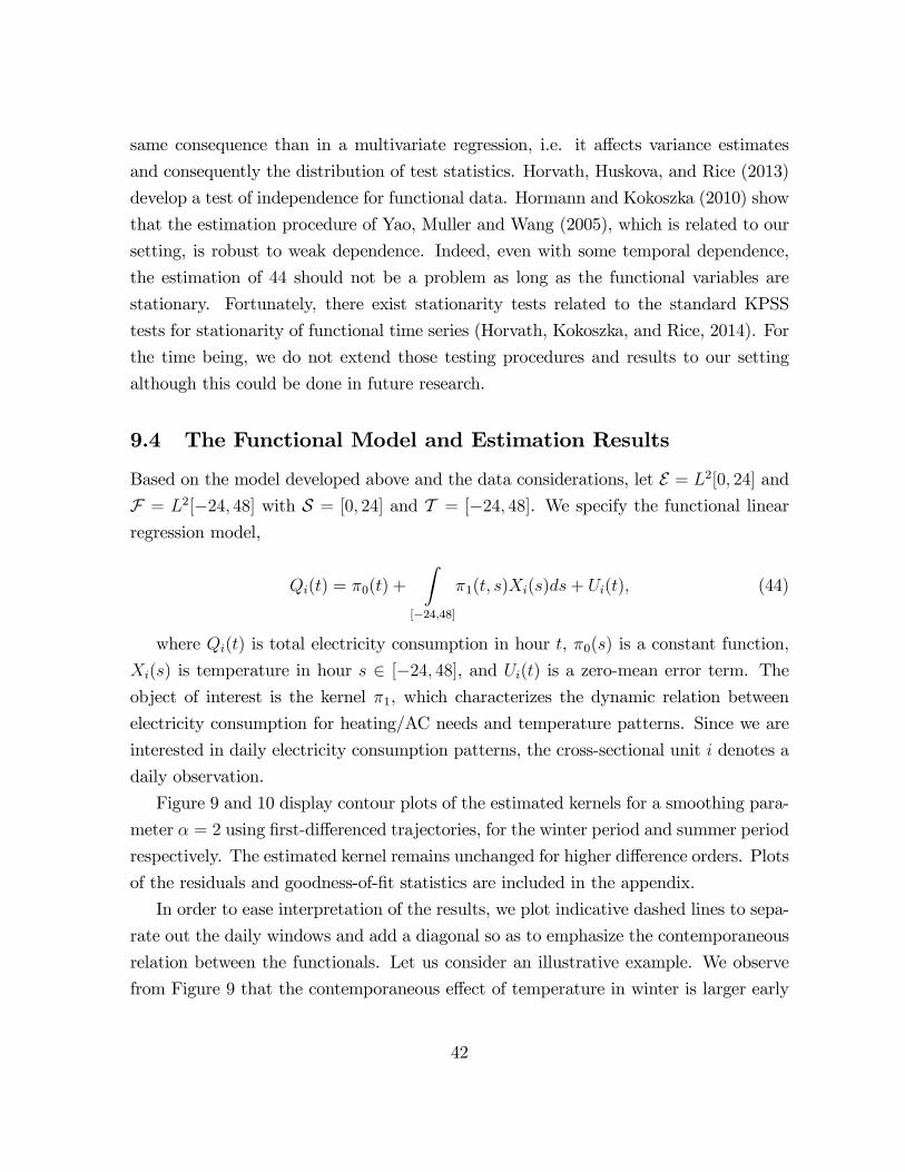
9.4 The Functional Model and Estimation Results

Based on the model developed above and the data considerations, let E = L2[0; 24] and

F = L2[�24; 48] with S = [0; 24] and T = [�24; 48]. We specify the functional linearregression model,

Qi(t) = �0(t) +

Z[�24;48]

�1(t; s)Xi(s)ds+ Ui(t); (44)

where Qi(t) is total electricity consumption in hour t, �0(s) is a constant function,

Xi(s) is temperature in hour s 2 [�24; 48], and Ui(t) is a zero-mean error term. Theobject of interest is the kernel �1, which characterizes the dynamic relation between

electricity consumption for heating/AC needs and temperature patterns. Since we are

interested in daily electricity consumption patterns, the cross-sectional unit i denotes a

daily observation.

Figure 9 and 10 display contour plots of the estimated kernels for a smoothing para-

meter � = 2 using �rst-di¤erenced trajectories, for the winter period and summer period

respectively. The estimated kernel remains unchanged for higher di¤erence orders. Plots

of the residuals and goodness-of-�t statistics are included in the appendix.

In order to ease interpretation of the results, we plot indicative dashed lines to sepa-

rate out the daily windows and add a diagonal so as to emphasize the contemporaneous

relation between the functionals. Let us consider an illustrative example. We observe

from Figure 9 that the contemporaneous e¤ect of temperature in winter is larger early

42

morning and in the afternoon (red regions); which correspond to the on-peak periods.

More generally, one can read the results both horizontally and vertically. The e¤ect of

the entire temperature pattern on electricity consumption at a given hour of the day is

observed horizontally, whereas the e¤ect of temperature at a speci�c time upon the daily

electricity consumption pattern is read vertically. The magnitudes of the correlation are

indicated using colors from dark blue to dark red with corresponding values given in

the legend. The seemingly S shape of the kernel around the indicative diagonal is likely

to be an artefact of the Tikhonov regularization, as observed in our simulations, and

consequently interpretative attempts of the results should account of this feature.

                    Day­1                    Day                    Day+1

Time (Temperature patterns)12AM 06AM 12PM 06PM 12AM 06AM 12PM 06PM 12AM 06AM 12PM 06PM 12AM

Tim

e (E

lect

ricity

 usa

ge p

atte

rns)

12AM

03AM

06AM

09AM

12PM

03PM

06PM

09PM

12AM

­2

­1

0

1

2

3

4

5

6

7

8

Figure 9: Contour plots of estimation results for winter months with � = 2

In general, we observe that the e¤ect of temperature on the consumption is of larger

magnitude in the summer period. Furthermore, the lagged and anticipatory e¤ects

appear to span over a longer interval around the diagonal. The red areas, where the

magnitude of the correlation is highest, show in particular that electricity consumption

from 2 am to 12 am strongly depends on temperatures from 7 pm to 12 am, suggesting

that consumers anticipate evening temperatures by turning up the A/C. Also, afternoon

43

consumption appears to depend on morning weather, suggesting the existence lag ef-

fects. Nevertheless, the kernel for summer is hard to interpret and statistical tests could

provide further insights on the results.

                    Day­1                    Day                    Day+1

Time (Temperature patterns)12AM 06AM 12PM 06PM 12AM 06AM 12PM 06PM 12AM 06AM 12PM 06PM 12AM

Tim

e (E

lect

ricity

 usa

ge p

atte

rns)

12AM

03AM

06AM

09AM

12PM

03PM

06PM

09PM

12AM

­5

0

5

10

15

20

25

Figure 10: Contour plots of estimation results for summer months with � = 2

Clearly, estimation results suggest the existence of both lag and anticipatory e¤ects.

Even for periods longer than a couple of hours. For instance in summer, the daily

consumption pattern appear to depend negatively, though to a relatively low extent,

on the day-after�s evening temperatures. This suggest that during the hot season when

temperatures are persistently high for days, consumers may choose to use less A/C. In

general, the estimated coe¢ cients of past, current and future values of temperature also

seem to vary greatly across hours of the day.

9.5 Conclusion of the application

This simple application sought to shed light on the potential uses of our estimator in

a di¤erent context than statistical prediction. The empirical analysis is based on a lin-

ear rational expectations model with perfect foresight. We use the functional model to

44

quantify the dynamic relationship between daily electricity consumption and tempera-

ture patterns in the province of Ontario. The data set consists of hourly consumption

and hourly temperature data at the province level. Results show that electricity con-

sumption decisions are subject to not only contemporaneous temperature but also past

and future realizations. This relation seems to di¤er for winter and summer months

and across hours of the day. When evaluating future temperatures, we use actual values

rather than expectations since short-term weather forecasts may be considered reason-

ably accurate.

A Appendix

12A M 03A M 06A M 09A M 12P M 03P M 06P M 09P M 12A M14

15

16

17

18

19

20

12A M 06A M 12P M 06P M 12A M 06A M 12P M 06P M 12A M 06A M 12P M 06P M 12A M0

5

10

15

20

25

30                    Day­1                    Day                    Day+1

Figure 11: Sample of levels for Thursdays (Winter)

45

12A M 03A M 06A M 09A M 12P M 03P M 06P M 09P M 12A M13

14

15

16

17

18

19

20

21

22

12A M 06A M 12P M 06P M 12A M 06A M 12P M 06P M 12A M 06A M 12P M 06P M 12A M10

12

14

16

18

20

22

24

26

28                    Day­1                    Day                    Day+1

Figure 12: Sample of levels for Thursdays (Summer)

10 20 30 40 50 60 70 80 90 100 110­1500

­1000

­500

0

500

1000

1500Residual from  levels

10 20 30 40 50 60 70 80 90 100 110­1500

­1000

­500

0

500

1000

1500

2000Residual fr om  first­differences

Figure 13: Residuals for series in levels and di¤erences (Winter)

10 20 30 40 50 60 70­1500

­1000

­500

0

500

1000

1500Residual from  levels

10 20 30 40 50 60­2000

­1500

­1000

­500

0

500

1000

1500

2000Residual from  fir st­differences

Figure 14: Residuals for series in levels and di¤erences (Summer)

46

12AM 03AM 06AM 09AM 12PM 03PM 06PM 09PM 12AM0

0.1

0.2

0.3

0.4

0.5

0.6

0.7

0.8

0.9

1

Figure 15: Coe¢ cients of determination (local and global) for series in levels and di¤er-ences (Winter)

12AM 03AM 06AM 09AM 12PM 03PM 06PM 09PM 12AM0

0.1

0.2

0.3

0.4

0.5

0.6

0.7

0.8

0.9

1

Figure 16: Coe¢ cients of determination (local and global) for series in levels and di¤er-ences (Summer)

47

B Proofs

Proof of Proposition 1.

�� 2HS

=

CY Z ��I + VZ

��1 2HS

� CY Z 2

HS

��I + VZ

��1 op

using the fact that, if A is a HS operator and B is a bounded operator, kABkHS �kAkHS kBkop where kBkop � supk�k�1 kB�k is the operator norm. Then, we have �� 2

HS� 1

�

CY Z 2HS

:

It remains to show that CY Z is a HS operator. CY Z is an integral operator with degen-

erate kernel 1n

Pni=1 yi (s) zi (t). A su¢ cient condition for CY Z to be HS is that its kernel

is square integrable which is true because Yi and Zi are elements of Hilbert spaces. The

result of Proposition 1 follows.

Proof of Proposition 2. To prove Proposition 2, we need two preliminary lemmas.

Lemma 7 Let A = B + C where B is a zero mean random operator and C is a non-

random operator. Then,

E�kAk2HS

�= E

�kBk2HS

�+ kCk2HS :

48

Proof of Lemma 7.

E�kAk2HS

�= E

Xj

A�j; A�j

�!

= E

Xj

A�A�j; �j

�!

= E

Xj

(B + C)� (B + C)�j; �j

�!

= E

Xj

B�B�j; �j

�!

+E

Xj

C�B�j; �j

�!

+E

Xj

B�C�j; �j

�!

+E

Xj

C�C�j; �j

�!:

The second and third terms on the r.h.s are equal to zero because E (B) = 0 and C is

deterministic. We obtain E�kAk2HS

�= E

�kBk2HS

�+ kCk2HS :

Lemma 8 Let A be a random operator from E to F .

E�kAk2HS

�= trE (A�A) :

Proof of Lemma 8. We have

E�kAk2HS

�= E

Xj

A�A�j; �j

�!=

Xj

E (A�A)�j; �j

�= trE (A�A) :

We turn to the proof of Proposition 2. Applying Lemma 7 on the decomposition

49

(12), (13), and (14), we have

E

� �� � � 2HSjZ1; Z2; :::; Zn

�= E

�k(12)k2HS jZ1; Z2; :::; Zn

�+ k(13) + (14)k2HS

� E�k(12)k2HS jZ1; Z2; :::; Zn

�+ 2 k(13)k2HS + 2 k(14)k

2HS :

We study the �rst term of the r.h.s. By Lemma 8,

E�k(12)k2HS jZ1; Z2; :::; Zn

�= E

��I + VZ

��1CZU

2HS

jZ1; Z2; :::; Zn

!

= trE

���I + VZ

��1CZU C

�ZU

��I + VZ

��1jZ1; Z2; :::; Zn

�= tr

���I + VZ

��1E�CZU C

�ZU jZ1; Z2; :::; Zn

���I + VZ

��1�:

Note that

CZU C�ZU' =

1

n2

Xi;j

zi hzj; 'i hui; uji ;

E�CZU C

�ZU'jZ1; Z2; :::; Zn

�=

1

n

Xi

zi hzi; 'iE [hui; uii jZ1; Z2; :::; Zn]

=1

n

Xi

zi hzi; 'i tr (VU)

=1

ntr (VU) VZ'

because the ui are uncorrelated. To see that E [hu; ui] = trVU , decompose u on the

basis formed by the eigenfunctions j of VU so that u =P

j

u; j

� j. It follows that

hu; ui =P

j

u; j

�2and E hu; ui =

Pj

VU j; j

�= tr (VU) : Hence,

E�k(12)k2HS jZ1; Z2; :::; Zn

�=

1

ntr (VU) tr

���I + VZ

��1VZ

��I + VZ

��1�� C

n�

50

where C is a generic constant. It follows that E�k(12)k2HS

�� C

n�:

Now, we turn toward the term (13). We have��I + VZ

��1VZ�

� � (�I + VZ)�1 VZ�

�

=

���I �

��I + VZ

��1VZ

�+�I � (�I + VZ)

�1 VZ����:

Using I =��I + VZ

��1 ��I + VZ

�, we obtain

I ���I + VZ

��1VZ = �

��I + VZ

��1:

Hence,

(13) =

�����I + VZ

��1+ � (�I + VZ)

�1���

=��I + VZ

��1 �VZ � VZ

�� (�I + VZ)

�1��

where the last equality follows from A�1 �B�1 = A�1 (A�B)B�1:

Now, we have ��I + VZ

��1 �VZ � VZ

�� (�I + VZ)

�1�� 2HS

� ��I + VZ

��1 2op

�VZ � VZ

� 2op

� (�I + VZ)�1��

2HS

where

��I + VZ

��1 2op

� 1=�2, �VZ � VZ

� 2op= Op (1=n) by Assumption 2 and � (�I + VZ)

�1�� 2HS= O

���^2

�:

If � > 1 then the term corresponding to (13) is negligeable with respect to (12). If

� < 1; then (12) is negligeable with respect to (13).

51

Now, we turn our attention toward the term (14). We have

(�I + VZ)�1 VZ�

� � ��

= (�I + VZ)�1 (VZ � �I � VZ)�

�

= � (�I + VZ)�1��

= � (�I + VZ)�1 V

�=2Z R

by Assumption 4. Let��j; 'j

be the eigenvalues and orthonormal eigenfunctions of

VZ : � (�I + VZ)�1 V

�=2Z R

2HS

= �2Xj

D(�I + VZ)

�1 V�=2Z R'j; (�I + VZ)

�1 V�=2Z R'j

E= �2

Xj

��j

(�j + �)2R'j; R'j

�2� �2 sup

�

��

(�+ �)2

Xj

R'j; R'j

�2= O

���^2

�:

The last equality follows from the fact thatP

j

R'j; R'j

�2= kRk2HS <1 and, using

the notation � = �2, we have

sup�

�2��

(�+ �)2= sup

�

�2�2�

(�2 + �)2= O

���^2

�by Carrasco, Florens, and Renault (2007, Proposition 3.11). Consequently, � (�I + VZ)

�1 V�=2Z R

2HS= O

���^2

�:

This concludes the proof of Proposition 2.

Proof of Proposition 5.We have

�m�� � �� = �m�� � ��� + ��� � ��:

52

We focus on the term �m�� � ���.

�m�� � ��� =��I + V m

Z

��1CmZY �

��I + VZ

��1CZY

=��I + V m

Z

��1 �CmZY � CZY

�+

���I + V m

Z

��1���I + VZ

��1�CZY :

CmZY � CZY

2HS

=

1nnXi=1

zmi hymi ; :i �1

n

nXi=1

zi hyi; :i 2

HS

=

1nnXi=1

f(zmi � zi) hyi; :i+ zmi hymi � yi; :ig 2

HS

� 2

n2

nXi=1

�k(zmi � zi) hyi; :ik2HS + kzmi hymi � yi; :ik2HS

:

k(zmi � zi) hyi; :ik2HS =Xj

(zmi � zi)

yi; �j

�; (zmi � zi)

yi; �j

��= kzmi � zik2

Xj

yi; �j

�2= Op

�f (m)2

�:

kzmi hymi � yi; :ik2HS =Xj

zmiymi � yi; �j

�; zmi

ymi � yi; �j

��= kzmi k

2Xj

ymi � yi; �j

�2= kzmi k

2 kymi � yik2

= Op�f (m)2

�:

Hence, ��I + V mZ

��1 �CmZY � CZY

� 2HS

= Op

f (m)2

�2n2

!:

53

���I + V m

Z

��1���I + VZ

��1�CZY

=��I + V m

Z

��1 �VZ � V m

Z

���I + VZ

��1CZY

=��I + V m

Z

��1 �VZ � V m

Z

����:

Hence, ��I + V mZ

��1 �VZ � V m

Z

����

2HS

= Op

f (m)2

�2n2

!:

This concludes the proof of Proposition 5.Proof of Proposition 6. Using the fact that ka+ b+ ck2HS � 3

�kak2HS + kbk

2HS + kck

2HS

�;

we can evaluate the terms (25), (26), and (27) separately. The proof follows closely that

of Proposition 2. Let Z andW be the sets (Z1; Z2; :::; Zn) and (W1;W2; :::;Wn) :

E�k(25)k2HS jZ;W

�= tr

���I + CZW CWZ

��1CZWE

�CWU CUW jZ;W

�CWZ

��I + CZW CWZ

��1�:

Using

E�CWU CUW jZ;W

�=1

ntr (VU) VW ;

we obtain

E�k(25)k2HS

�� C

n�

for some constant C:

The proof regarding the rates of convergence of (26) and (27) is similar to that of

Proposition 2 and is not repeated here.

54

REFERENCES

Andersson, J. and J. Lillestol, 2010. Modeling and forecasting electricity consuption by

functional data analysis. The Journal of Energy Markets, 3:315.

Antoch, J., L. Prchal, M. De Rosa, and P. Sarda, 2010, Electricity consumption pre-

diction with functional linear regression using spline estimators, Journal of Applied

Statistics, 37, 2027-2041.

Bosq, D. Linear processes in function spaces: Theory and applications. Springer-Verlag,

New York, 2000.

Breunig, C. and Johannes, J. ,2015, Adaptive estimation of functionals in nonparametric

instrumental regression. forthcoming in Econometric Theory (arXiv:1109.0961)

Cardo, H., F. Ferraty, and P. Sarda (2003) Spline estimators for the functional linear

model, Statistica Sinica, 13, 571-591.

Carrasco, M. and J. P. Florens, 2000, Generalization of GMM to a continuum of moment

conditions. Econometric Theory, 16, 797-834.

Carrasco, M., J. P. Florens, and E. Renault, 2007, Linear Inverse Problems in Struc-

tural Econometrics: Estimation based on spectral decomposition and regularization,

Handbook of Econometrics, Vol. 6B, edited by J.J. Heckman and E.E. Leamer.

Centorrino, S., 2014, Data-driven selection of the regularization parameter in additive

nonparametric instrumental regressions, mimeo, Stony Brook University.

Centorrino, S. and J.-P. Florens, 2014, Nonparametric instrumental variable estimation

of binary response models, mimeo, Stony Brook University.

Centorrino, S., F. Fève, and J.-P. Florens, 2013, Implementation simulations and boot-

strap in nonparametric instrumental variable estimation, mimeo, Stony Brook Univer-

sity.

Comte and Johannes (2012) Adaptive functional linear regression. Annals of Statistics,

40(6), 2765-2797

Conley, T., L. Hansen, E. Luttmer, J. Scheinkman (1997) Short-Term Interest Rates as

Subordinated Di¤usions, The Review of Financial Studies, 10(3).

Crambes, C, A. Kneip, and P. Sarda, 2009, Smoothing spline estimators for functional

linear regression, The Annals of Statistics, 37, 35-72.

Crambes, C. and A. Mas, 2013, Asymptotics of prediction in functional linear regression

with functional outputs, Bernoulli, 19, 2627-2651.

55

Cuevas, A., M. Febrero, and R. Fraiman, 2002, Linear functional regression: the case of

�xe design and functional response. The Canadian Journal of Statistics. Vol 30., N.2,

285-300.

Darolles, S., Y. Fan, J.-P. Florens, and E. Renault, 2011, Nonparametric Instrumental

Regression, Econometrica, 79, 1541-1565.

Dauxois, J., A. Pousse, and Y. Romain, 1982, Asymptotic Theory for the Principal

Component Analysis of a Vector Random Function: Some Applications to Statistical

Inference, Journal of Multivariate Analysis, 12, 136-154.

Engl, H., M. Hanke, and A. Neubauer, 2000, Regularization of Inverse Problems, Kluwer

Academic Publishers, Dordrecht.

Eubank, R., 1988, Spline Smoothing and Nonparametric Regression, Marcel Dekker,

New York.

Faruqui, A., S. Sergici, N. Lessem, F. Denton, B. Spencer, and C. King (2013) Report

prepared for Ontario Power Authority, Impact Evaluation of Ontario�s Time-of-Use

Rates: First Year Analysis.

Ferraty, F. and P. Vieu, 2006, Nonparametric Functional Data Analysis: Methods, The-

ory, Applications and Implementations, Springer-Verlag, London.

Gabrys, R., L. Horvath, and P. Kokoszka, 2010, Tests for Error Correlation in the

Functional Linear Model, Journal of the American Statistical Association, 105:491, 1113-

1125.

Goldenshluger and Lepski (2011) Bandwidth selection in kernel density estimation: or-

acle inequalities and adaptive minimax optimality. Annals of Statistics, 39, 1608-1632.

Hall, P. and J. Horowitz, 2007, Methodology and convergence rates for functional linear

regression, The Annals of Statistics, 35, 70-91.

Hansen, L.P. and T. Sargent, 1980. Formulating and estimating dynamic linear rational

expectations models, Journal of Economic Dynamics and Control, Elsevier, vol. 2(1),

pages 7-46.

Hansen, L.P. and T. Sargent, 1982. Formulating and estimating continuous time rational

expectations models, Sta¤ Report 75, Federal Reserve Bank of Minneapolis.

Hansen, L.P. and T. Sargent, 1983. Identi�cation of continuous time rational expecta-

tions models from discrete time data, Sta¤ Report 73, Federal Reserve Bank of Min-

neapolis.

Harmann, S., Kokoszka, P., 2010. Weakly dependent functional data. Ann. Statist. 38,

56

1845-1884.

Harmann, S., Kokoszka, P., 2012. Functional time series. In: Rao, C.R., Subba Rao, T.

(Eds.), Handbook of Statistics. In: Time Series, vol. 30. Elsevier.

He, G., H. G. Müller, and J. L. Wang, 2000, Extending Correlation and Regression from

Multivariate to Functional Data, Asymptotics in Statistics and Probability, 1-14.

Horowitz, J. and S. Lee, 2007, Nonparametric Instrumental Variables Estimation of a

Quantile Regression Model, Econometrica, Vol. 75, No. 4, 1191-1208.

Horvath, L. and P. Kokoszka, 2012. Inference for Functional Data with Applications,

Springer, New York, NY, USA.

Horvath, L., M. Huskova and G. Rice, 2013. Test of independence for functional data,

Journal of Multivariate Analysis, Elsevier, vol. 117(C), pages 100-119.

Horvath, L., P. Kokoszka and G. Rice, 2014. Testing stationarity of functional time

series, Journal of Econometrics, Elsevier, vol. 179(1), pages 66-82.

Kennan, J. (1979), The Estimation of Partial Adjustment Models with Rational Expec-

tations, Econometrica, vol.47

Kress, R. (1999), Linear Integral Equations, Springer.

Liebl, D. Modeling and forecasting electricity spot prices: A functional data perspective.

Ann. Appl. Stat. 7 (2013), no. 3, 1562�1592.

McLaughlin, L., Jia, L., Yu, Z. and Tong, L., 2011, Thermal Dynamic for Home Energy

Management: A Case Study. Cornell Univ., Ithaca, NY, USA, Tech. Rep. ACSP-TR-

10-11-01.

Muth, J. (1961). "Rational Expectations and the Theory of Price Movements", Econo-

metrica 29, pp. 315-335.

Patrick, R. and F. Wolak. 1997. Estimating customer-level demand for electricity under

real time pricing. Document available from http://www.stanford.edu/-wolak.

Ramsay, J.O. and B.W. Silverman, 2005, Functional Data Analysis, 2nd edition, Springer,

New York.

Rudin, W., 1991. Functional Analysis, 2nd Edition, McGraw Hill.

Vilenkin, N.I.A, 1968. Special functions and the theory of group representations, Amer-

ican Mathematical Society.

Weron, R. 2006. "Modeling and Forecasting Electricity Loads and Prices: A Statistical

Approach," HSC Books, Hugo Steinhaus Center, Wroclaw University of Technology.

Statistics Canada, 2008, EnviroStats "Thermostat use in Canadian homes". Fall 2008

57

Vol.2, no.3, Catalogue no.16-002-X.

Yao, F., H. G. Müller, and J. L. Wang, 2005, Functional Linear Regression Analysis for

Longitudinal Data, The Annals of Statistics, Vol. 33, N.6, 2873-2903.

Yu, Z., McLaughlin, L., Jia, L., Murphy-Hoye, M.C., Pratt, A. and Tong, L., 2012,

Modeling and Stochastic Control for Home Energy Management. Proc. IEEE PES

Gen. Meet., July.

58