Functional It calculus and stochastic integral ...2013, Vol. 41, No. 1, 109–133 DOI: 10.1214/11-AOP721 c Institute of Mathematical Statistics, 2013 FUNCTIONAL ITO CALCULUS AND ... ·

arX

iv:1

002.

2446

v5 [

mat

h.PR

] 4

Feb

201

3

The Annals of Probability

2013, Vol. 41, No. 1, 109–133DOI: 10.1214/11-AOP721c© Institute of Mathematical Statistics, 2013

FUNCTIONAL ITO CALCULUS AND

STOCHASTIC INTEGRAL REPRESENTATION OF MARTINGALES

By Rama Cont and David-Antoine Fournie

CNRS—Universite Pierre & Marie Curie and Columbia University

We develop a nonanticipative calculus for functionals of a contin-uous semimartingale, using an extension of the Ito formula to path-dependent functionals which possess certain directional derivatives.The construction is based on a pathwise derivative, introduced byDupire, for functionals on the space of right-continuous functions withleft limits. We show that this functional derivative admits a suitableextension to the space of square-integrable martingales. This exten-sion defines a weak derivative which is shown to be the inverse of theIto integral and which may be viewed as a nonanticipative “lifting”of the Malliavin derivative.

These results lead to a constructive martingale representationformula for Ito processes. By contrast with the Clark–Haussmann–Ocone formula, this representation only involves nonanticipative quan-tities which may be computed pathwise.

1. Introduction. In the analysis of phenomena with stochastic dynam-ics, Ito’s stochastic calculus [8, 15, 16, 19, 23, 28, 29] has proven to be apowerful and useful tool. A central ingredient of this calculus is the Itoformula [15, 16, 23], a change of variable formula for functions f(Xt) of asemimartingale X which allows one to represent such quantities in termsof a stochastic integral. Given that in many applications such as statisticsof processes, physics or mathematical finance, one is led to consider path-dependent functionals of a semimartingale X and its quadratic variationprocess [X] such as

∫ t

0g(t,Xt)d[X](t), G(t,Xt, [X]t), or E[G(T,X(T ), [X](T ))|Ft ](1)

Received February 2010; revised September 2011.AMS 2000 subject classifications. 60H05, 60H07, 60G44, 60H25.Key words and phrases. Stochastic calculus, functional calculus, functional Ito for-

mula, Malliavin derivative, martingale representation, semimartingale, Wiener functionals,Clark–Ocone formula.

This is an electronic reprint of the original article published by theInstitute of Mathematical Statistics in The Annals of Probability,2013, Vol. 41, No. 1, 109–133. This reprint differs from the original in paginationand typographic detail.

1

http://arxiv.org/abs/1002.2446v5

http://www.imstat.org/aop/

http://dx.doi.org/10.1214/11-AOP721

http://www.imstat.org

http://www.ams.org/msc/

http://www.imstat.org

http://www.imstat.org/aop/

http://dx.doi.org/10.1214/11-AOP721

2 R. CONT AND D.-A. FOURNIE

(where X(t) denotes the value at time t and Xt = (X(u), u ∈ [0, t]) the pathup to time t), there has been a sustained interest in extending the frameworkof stochastic calculus to such path-dependent functionals.

In this context, the Malliavin calculus [3, 22, 24, 25, 30–32] has provento be a powerful tool for investigating various properties of Brownian func-tionals. Since the construction of Malliavin derivative does not refer to anunderlying filtration Ft, it naturally leads to representations of functionalsin terms of anticipative processes [4, 14, 25]. However, in most applications itis more natural to consider nonanticipative versions of such representations.

In a recent insightful work, Dupire [9] has proposed a method to extendthe Ito formula to a functional setting using a pathwise functional deriva-tive which quantifies the sensitivity of a functional Ft :D([0, t],R)→ R to avariation in the endpoint of a path ω ∈D([0, t],R).

∇ωFt(ω) = limε→0

Ft(ω + ε1t)−Ft(ω)

ε.

Building on this insight, we develop hereafter a nonanticipative calcu-lus [5] for a class of processes—including the above examples—which maybe represented as

Y (t) = Ft(X(u),0≤ u≤ t,A(u),0≤ u≤ t) = Ft(Xt,At),(2)

where A is the local quadratic variation defined by [X](t) =∫ t0 A(u)du, and

the functional

Ft :D([0, t],Rd)×D([0, t], S+d )→R

represents the dependence of Y on the path Xt = X(u),0 ≤ u ≤ t of Xand its quadratic variation.

Our first result (Theorem 4.1) is a change of variable formula for path-dependent functionals of the form (2). Introducing At as an additional vari-able allows us to control the dependence of Y with respect to the “quadraticvariation” [X] by requiring smoothness properties of Ft with respect to thevariable At in the supremum norm, without resorting to p-variation normsas in “rough path” theory [20]. This allows our result to cover a wide rangeof functionals, including the examples in (1).

We then extend this notion of functional derivative to processes: we showthat for Y of the form (2) where F satisfies some regularity conditions, theprocess ∇XY =∇ωF (Xt,At) may be defined intrinsically, independently ofthe choice of F in (2). The operator ∇X is shown to admit an extension tothe space of square-integrable martingales, which is the inverse of the Itointegral with respect to X : for φ ∈ L2(X),∇X(

∫

φ · dX) = φ (Theorem 5.8).In particular, we obtain a constructive version of the martingale represen-tation theorem (Theorem 5.9), which states that for any square-integrable

FUNCTIONAL ITO CALCULUS 3

FXt -martingale Y ,

Y (T ) = Y (0) +

∫ T

0∇XY · dX, P-a.s.

This formula can be seen as a nonanticipative counterpart of the Clark–Haussmann–Ocone formula [4, 13, 14, 18, 25]. The integrand ∇XY is anadapted process which may be computed pathwise, so this formula is moreamenable to numerical computations than those based on Malliavin calculus.

Finally, we show that this functional derivative ∇X may be viewed asa nonanticipative “lifting” of the Malliavin derivative (Theorem 6.1): forsquare-integrable martingales Y whose terminal values is differentiable inthe sense of Malliavin Y (T ) ∈D

1,2, we show that ∇XY (t) =E[DtH|Ft].These results provide a rigorous mathematical framework for developing

and extending the ideas proposed by Dupire [9] for a large class of func-tionals. In particular, unlike the results derived from the pathwise approachpresented in [6, 9], Theorems 5.8 and 5.9 do not require any pathwise regu-larity of the functionals and hold for nonanticipative square-integrable pro-cesses, including stochastic integrals and functionals which may depend onthe quadratic variation of the process.

2. Functional representation of nonanticipative processes. LetX : [0, T ]×Ω 7→ Rd be a continuous, Rd-valued semimartingale defined on a filteredprobability space (Ω,F ,Ft,P) assumed to satisfy the usual hypotheses [8].Denote by P (resp., O) the associated predictable (resp., optional) sigma-algebra on [0, T ]. FX

t denotes the (P-completed) natural filtration of X . Thepaths of X then lie in C0([0, T ],R

d), which we will view as a subspace ofD([0, T ],Rd) the space of cadlag functions with values in Rd. We denote by[X] = ([Xi,Xj ], i, j = 1, . . . , d) the quadratic (co-)variation process associ-ated to X , taking values in the set S+

d of positive d×d matrices. We assumethat

[X](t) =

∫ t

0A(s)ds(3)

for some cadlag process A with values in S+d . Note that A need not be a

semimartingale. The paths of A lie in St =D([0, t], S+d ), the space of cadlag

functions with values S+d .

2.1. Horizontal extension and vertical perturbation of a path. Considera path x ∈D([0, T ]),Rd) and denote by xt = (x(u),0≤ u≤ t) ∈D([0, t],Rd)its restriction to [0, t] for t < T . For a process X we shall similarly denoteX(t) its value at t and Xt = (X(u),0≤ u≤ t) its path on [0, t].

For h≥ 0, we define the horizontal extension xt,h ∈D([0, t+ h],Rd) of xtto [0, t+ h] as

xt,h(u) = x(u), u ∈ [0, t]; xt,h(u) = x(t), u ∈ ]t, t+ h].(4)


For h ∈Rd, we define the vertical perturbation xht of xt as the cadlag pathobtained by shifting the endpoint by h.

xht (u) = xt(u), u ∈ [0, t[, xht (t) = x(t) + h,(5)

or, in other words, xht (u) = xt(u) + h1t=u.

2.2. Adapted processes as nonanticipative functionals. A process Y :[0, T ]×Ω 7→Rd adapted to FX

t may be represented as

Y (t) = Ft(X(u),0≤ u≤ t,A(u),0≤ u≤ t) = Ft(Xt,At),(6)

where F = (Ft)t∈[0,T ] is a family of functionals

Ft :D([0, t],Rd)×St →R

representing the dependence of Y (t) on the underlying path of X and itsquadratic variation.

Since Y is nonanticipative, Y (t,ω) only depends on the restriction ωt ofω on [0, t]. This motivates the following definition:

Definition 2.1 (Nonanticipative functional). A nonanticipative func-tional is a family of functionals F = (Ft)t∈[0,T ] where

Ft :D([0, t],Rd)×D([0, t], S+d ) 7→ R,

(x, v)→ Ft(x, v)

is measurable with respect to Bt, the canonical filtration on D([0, t],Rd)×D([0, t], S+

d ).

We can also view F = (Ft)t∈[0,T ] as a map defined on the space Υ ofstopped paths

Υ= (t,ωt,T−t), (t,ω) ∈ [0, T ]×D([0, T ],Rd × S+d ).(7)

Whenever the context is clear, we will denote a generic element (t,ω) ∈ Υsimply by its second component, the path ω stopped at t. Υ can also beidentified with the “vector bundle”

Λ =⋃

t∈[0,T ]

D([0, t],Rd)×D([0, t], S+d ).(8)

A natural distance on the space Υ of stopped paths is given by

d∞((t,ω), (t′, ω′)) = |t− t′|+ supu∈[0,T ]

|ωt,T−t(u)− ω′t′,T−t′(u)|.(9)

(Υ, d∞) is then a metric space, a closed subspace of ([0, T ]×D([0, T ],Rd ×S+d ),‖ · ‖∞) for the product topology.


Introducing the process A as an additional variable may seem redundantat this stage: indeed A(t) is itself Ft-measurable, that is, a functional of Xt.However, it is not a continuous functional on (Υ, d∞). Introducing At asa second argument in the functional will allow us to control the regularityof Y with respect to [X]t =

∫ t0 A(u)du simply by requiring continuity of Ft

in supremum or Lp norms with respect to the “lifted process” (X,A); seeSection 2.3. This idea is analogous in some ways to the approach of roughpath theory [20], although here we do not resort to p-variation norms.

If Y is a Bt-predictable process, then [8, Volume I, paragraph 97]

∀t ∈ [0, T ], Y (t,ω) = Y (t,ωt−),

where ωt− denotes the path defined on [0, t] by

ωt−(u) = ω(u), u ∈ [0, t[, ωt−(t) = ω(t−).

Note that ωt− is cadlag and should not be confused with the caglad pathu 7→ ω(u−).

The functionals discussed in the introduction depend on the process Avia [X] =

∫ ·0A(t)dt. In particular, they satisfy the condition Ft(Xt,At) =

Ft(Xt,At−). Accordingly, we will assume throughout the paper that all func-tionals Ft :D([0, t],Rd)×St →R considered have “predictable” dependencewith respect to the second argument,

∀t ∈ [0, T ],∀(x, v) ∈D([0, t],Rd)×St, Ft(xt, vt) = Ft(xt, vt−).(10)

2.3. Continuity for nonanticipative functionals. We now define a notionof (left) continuity for nonanticipative functionals.

Definition 2.2 (Continuity at fixed times). A functional F defined onΥ is said to be continuous at fixed times for the d∞ metric if and only if

∀t ∈ [0, T ),∀ε > 0,∀(x, v) ∈D([0, t],Rd)×St,

∃η > 0, (x′, v′) ∈D([0, t],Rd)×St,(11)

d∞((x, v), (x′, v′))< η ⇒ |Ft(x, v)−Ft(x′, v′)|< ε.

We now define a notion of joint continuity with respect to time and theunderlying path:

Definition 2.3 (Continuous functionals). A nonanticipative functionalF = (Ft)t∈[0,T ) is said to be continuous at (x, v) ∈D([0, t],Rd)×St if

∀ε > 0,∃η > 0,∀(x′, v′) ∈Υ,(12)

d∞((x, v), (x′, v′))< η ⇒ |Ft(x, v)−Ft′(x′, v′)|< ε.

We denote by C0,0([0, T )) the set of continuous nonanticipative functionalson Υ.


Definition 2.4 (Left-continuous functionals). A nonanticipative func-tional F = (Ft, t ∈ [0, T )) is said to be left-continuous if for each t ∈ [0, T ),Ft :D([0, t],Rd)×St →R in the sup norm and

∀ε > 0,∀(x, v) ∈D([0, t],Rd)×St,

∃η > 0,∀h ∈ [0, t],∀(x′, v′) ∈D([0, t− h],Rd)×St−h,(13)

d∞((x, v), (x′, v′))< η ⇒ |Ft(x, v)− Ft−h(x′, v′)|< ε.

We denote by C0,0l ([0, T )) the set of left-continuous functionals.

We define analogously the class of right-continuous functionals C0,0r ([0, T )).

We call a functional “boundedness preserving” if it is bounded on eachbounded set of paths:

Definition 2.5 (Boundedness-preserving functionals). Define B([0, T ))as the set of nonanticipative functionals F such that for every compactsubset K of Rd, every R> 0 and t0 < T ,

∃CK,R,t0 > 0,∀t≤ t0,∀(x, v) ∈D([0, t],K)×St,(14)

sups∈[0,t]

|v(s)|<R ⇒ |Ft(x, v)|<CK,R,t0 .

2.4. Measurability properties. Composing a nonanticipative functional Fwith the process (X,A) yields an Ft-adapted process Y (t) = Ft(Xt,At). Theresults below link the measurability and pathwise regularity of Y to theregularity of the functional F .

Lemma 2.6 (Pathwise regularity). If F ∈ C0,0l , then for any (x, v) ∈

D([0, T ],Rd)×ST , the path t 7→ Ft(xt−, vt−) is left-continuous.

Proof. Let F ∈C0,0l and t ∈ [0, T ). For h > 0 sufficiently small,

d∞((xt−h, vt−h), (xt−, vt−)) = supu∈(t−h,t)

|x(u)− x(t− h)|

(15)+ supu∈(t−h,t)

|v(u)− v(t− h)|+ h.

Since x and v are cadlag, this quantity converges to 0 as h→ 0+, so

Ft−h(xt−h, vt−h)− Ft(xt−, vt−)h→0+→ 0,

so t 7→ Ft(xt−, vt−) is left-continuous.

Theorem 2.7. (i) If F is continuous at fixed times, then the process Ydefined by Y ((x, v), t) = Ft(xt, vt) is adapted.


(ii) If F ∈C0,0l ([0, T )), then the process Z(t) = Ft(Xt,At) is optional.

(iii) If F ∈C0,0l ([0, T )), and if either A is continuous or F verifies (10),

then Z is a predictable process.

In particular, any F ∈C0,0l is a nonanticipative functional in the sense of

Definition 2.1. We propose an easy-to-read proof of points (i) and (iii) in thecase where A is continuous. The (more technical) proof for the cadlag caseis given in the Appendix.

Continuous case. Assume that F is continuous at fixed times and thatthe paths of (X,A) are almost-surely continuous. Let us prove that Y is Ft-adapted: X(t) is Ft-measurable. Introduce the partition tin =

iT2n , i= 0, . . . ,2n

of [0, T ], as well as the following piecewise-constant approximations of Xand A:

Xn(t) =2n∑

k=0

X(tnk )1[tnk ,tnk+1)

(t) +XT 1T(t),

(16)

An(t) =

2n∑

k=0

A(tnk )1[tnk ,tnk+1)

(t) +AT 1T(t).

The random variable Y n(t) = Ft(Xnt ,A

nt ) is a continuous function of the

random variables X(tnk ),A(tnk ), t

nk ≤ t and hence is Ft-measurable. The

representation above shows in fact that Y n(t) is Ft-measurable. Xnt and Ant

converge respectively to Xt and At almost-surely so Y n(t)→n→∞ Y (t) a.s.,and hence Y (t) is Ft-measurable.

(i) implies point (iii) since the path of Z are left-continuous by Lemma 2.6.

3. Pathwise derivatives of nonanticipative functionals.

3.1. Horizontal and vertical derivatives. We now define pathwise deriva-tives for a nonanticipative functional, following Dupire [9].

Definition 3.1 (Horizontal derivative). The horizontal derivative at(x, v) ∈D([0, t],Rd)×St of nonanticipative functional F = (Ft)t∈[0,T ) is de-fined as

DtF (x, v) = limh→0+

Ft+h(xt,h, vt,h)−Ft(xt, vt)

h(17)

if the corresponding limit exists. If (17) is defined for all (x, v) ∈Υ, the map

DtF :D([0, t],Rd)×St 7→Rd,(18)

(x, v)→DtF (x, v)

defines a nonanticipative functional DF = (DtF )t∈[0,T ], the horizontal deriva-tive of F .


Note that our definition (17) is different from the one in [9] where thecase F (x, v) =G(x) is considered.

Dupire [9] also introduced a pathwise spatial derivative for such func-tionals, which we now introduce. Denote (ei, i= 1, . . . , d) the canonical basisin Rd.

Definition 3.2. A nonanticipative functional F = (Ft)t∈[0,T ) is said to

be vertically differentiable at (x, v) ∈D([0, t]),Rd)×D([0, t], S+d ) if

Rd 7→ R,

e→ Ft(xet , vt)

is differentiable at 0. Its gradient at 0,

∇xFt(x, v) = (∂iFt(x, v), i= 1, . . . , d)(19)

where ∂iFt(x, v) = limh→0

Ft(xheit , v)−Ft(x, v)

h

is called the vertical derivative of Ft at (x, v). If (19) is defined for all (x, v) ∈Υ, the maps

∇xF :D([0, t],Rd)×St 7→Rd,(20)

(x, v)→∇xFt(x, v)

define a nonanticipative functional ∇xF = (∇xFt)t∈[0,T ], the vertical deriva-tive of F . F is then said to be vertically differentiable on Υ.

Remark 3.3. ∂iFt(x, v) is simply the directional derivative of Ft in thedirection (1tei,0). Note that this involves evaluating F at cadlag pertur-bations of the path x, even if x is continuous.

Remark 3.4. If Ft(x, v) = f(t, x(t)) with f ∈C1,1([0, T )×Rd), then weretrieve the usual partial derivatives

DtF (x, v) = ∂tf(t,X(t)), ∇xFt(Xt,At) =∇xf(t,X(t)).

Remark 3.5. Bismut [3] considered directional derivatives of function-als on D([0, T ],Rd) in the direction of purely discontinuous (e.g., piecewiseconstant) functions with finite variation, which is similar to Definition 3.2.This notion, used in [3] to derive an integration by parts formula for pure-jump processes, is natural in the context of discontinuous semimartingales.We will show that the directional derivative (19) also intervenes naturallywhen the underlying process X is continuous, which is less obvious.

Definition 3.6 (Regular functionals). Define C1,k([0, T )) as the set of

functionals F ∈C0,0l which are:


• horizontally differentiable with DtF continuous at fixed times;• k times vertically differentiable with ∇j

xF ∈C0,0l ([0, T )) for j = 1, . . . , k.

Define C1,kb ([0, T )) as the set of functionals F ∈C1,2 such that DF,∇xF, . . . ,

∇kxF ∈ B([0, T )).

We denote C1,∞([0, T )) =⋂

k≥1C1,k([0, T ).

Note that this notion of regularity only involves directional derivativeswith respect to local perturbations of paths, so ∇xF and DtF seems to con-tain less information on the behavior of F than, say, the Frechet derivativewhich considers perturbations in all directions in C0([0, T ],R

d) or the Malli-avin derivative [21, 22] which examines perturbations in the direction of allabsolutely continuous functions. Nevertheless we will show in Section 4 thatknowledge of DF,∇xF,∇

2xF along the paths of X is sufficient to reconstitute

the path of Y (t) = Ft(Xt,At).

Example 1 (Smooth functions). In the case where F reduces to asmooth function of X(t),

Ft(xt, vt) = f(t, x(t)),(21)

where f ∈ C1,k([0, T ] × Rd), the pathwise derivatives reduce to the usualones

DtF (xt, vt) = ∂tf(t, x(t)), ∇jxFt(xt, vt) = ∂jxf(t, x(t)).(22)

In fact to have F ∈ C1,k we just need f to be right-differentiable in thetime variable, with right-derivative ∂tf(t, ·) which is continuous in the spacevariable and f , ∇f and ∇2f to be jointly left-continuous in t and continuousin the space variable.

Example 2 (Cylindrical functionals). Let g ∈C0(Rd,R), h ∈ Ck(Rd,R)with h(0) = 0. Then

Ft(ω) = h(ω(t)− ω(tn−))1t≥tng(ω(t1−), ω(t2−), . . . , ω(tn−))

is in C1,kb with DtF (ω) = 0 and

∀j = 1, . . . , k,

∇jωFt(ω) = h(j)(ω(t)− ω(tn−))1t≥tng(ω(t1−), ω(t2−) . . . , ω(tn−)).

Example 3 (Integrals with respect to quadratic variation). A process

Y (t) =∫ t0 g(X(u))d[X](u) where g ∈ C0(Rd) may be represented by the

functional

Ft(xt, vt) =

∫ t

0g(x(u))v(u)du.(23)


It is readily observed that F ∈C1,∞b , with

DtF (xt, vt) = g(x(t))v(t), ∇jxFt(xt, vt) = 0.(24)

Example 4. The martingale Y (t) =X(t)2− [X](t) is represented by thefunctional

Ft(xt, vt) = x(t)2 −

∫ t

0v(u)du.(25)

Then F ∈C1,∞b with

DtF (x, v) =−v(t), ∇xFt(xt, vt) = 2x(t),(26)

∇2xFt(xt, vt) = 2, ∇j

xFt(xt, vt) = 0, j ≥ 3.

Example 5. Y = exp(X − [X]/2) may be represented as Y (t) = F (Xt)

Ft(xt, vt) = ex(t)−1/2∫ t

0v(u)du.(27)

Elementary computations show that F ∈C1,∞b with

DtF (x, v) =−1

2v(t)Ft(x, v), ∇j

xFt(xt, vt) = Ft(xt, vt).(28)

Note that, although At may be expressed as a functional of Xt, this func-tional is not continuous and without introducing the second variable v ∈ St,it is not possible to represent Examples 3, 4 and 5 as a left-continuous func-tional of x alone.

3.2. Obstructions to regularity. It is instructive to observe what preventsa functional from being regular in the sense of Definition 3.6. The examplesbelow illustrate the fundamental obstructions to regularity:

Example 6 (Delayed functionals). Let ε > 0. Ft(xt, vt) = x(t−ε) defines

a C0,∞b functional. All vertical derivatives are 0. However, F fails to be

horizontally differentiable.

Example 7 (Jump of x at the current time). Ft(xt, vt) = x(t)− x(t−)defines a functional which is infinitely differentiable and has regular pathwisederivatives

DtF (xt, vt) = 0, ∇xFt(xt, vt) = 1.(29)

However, the functional itself fails to be C0,0l .

Example 8 (Jump of x at a fixed time). Ft(xt, vt) = 1t≥t0(x(t0)−x(t0−))

defines a functional in C0,0l which admits horizontal and vertical derivatives

at any order at each point (x, v). However, ∇xFt(xt, vt) = 1t=t0 fails to beeither right- or left-continuous, so F is not C0,1 in the sense of Definition 3.2.


Example 9 (Maximum). Ft(xt, vt) = sups≤t x(s) is C0,0l but fails to be

vertically differentiable on the set

(xt, vt) ∈D([0, t],Rd)×St, x(t) = sups≤t

x(s)

.

4. Functional Ito calculus.

4.1. Functional Ito formula. We are now ready to prove our first mainresult, which is a change of variable formula for nonanticipative functionalsof a semimartingale [5, 9]:

Theorem 4.1. For any nonanticipative functional F ∈ C1,2b verifying

(10) and any t ∈ [0, T ),

Ft(Xt,At)− F0(X0,A0)

=

∫ t

0DuF (Xu,Au)du+

∫ t

0∇xFu(Xu,Au) · dX(u)(30)

+

∫ t

0

1

2tr(∇2

xFu(Xu,Au)d[X](u)) a.s.

In particular, for any F ∈C1,2b , Y (t) = Ft(Xt,At) is a semimartingale.

Theorem 4.1 shows that, for a regular functional F ∈C1,2([0, T )), the pro-cess Y = F (X,A) may be reconstructed from the second-order jet (DF,∇xF,∇2xF ) of F along the paths of X .

Proof. Let us first assume that X does not exit a compact set K andthat ‖A‖∞ ≤ R for some R > 0. Let us introduce a sequence of randompartitions (τnk , k = 0, . . . , k(n)) of [0, t], by adding the jump times of A to thedyadic partition (tni =

it2n , i= 0, . . . ,2n),

τn0 = 0, τnk = inf

s > τnk−1|2ns ∈N or |A(s)−A(s−)|>

1

n

∧ t.(31)

The following arguments apply pathwise. Lemma A.3 ensures that

ηn = sup

|A(u)−A(τni )|+ |X(u)−X(τni )|+t

2n, i≤ 2n, u ∈ [τni , τ

ni+1)

→n→∞

0.

Denote nX =∑∞

i=0X(τni+1)1[τni ,τni+1)+X(t)1t which is a cadlag piecewise

constant approximation of Xt, and nA =∑∞

i=0A(τni )1[τni ,τni+1)

+ A(t)1twhich is an adapted cadlag piecewise constant approximation of At. Denote


hni = τni+1 − τni . Start with the decomposition

Fτni+1(nXτni+1−

,nAτni+1−)− Fτni (nXτni −,nAτni −)

= Fτni+1(nXτni+1−

,nAτni ,hni )− Fτni (nXτni,nAτni )(32)

+ Fτni (nXτni,nAτni −)−Fτni (nXτni −,nAτni −),

where we have used the fact that F has predictable dependence in the secondvariable to have Fτni (nXτni

,nAτni ) = Fτni (nXτni,nAτni −). The first term in (32)

can be written ψ(hni )− ψ(0) where

ψ(u) = Fτni +u(nXτni ,u,nAτni ,u).(33)

Since F ∈ C1,2([0, T ]), ψ is right-differentiable and left-continuous by Lem-ma 2.6, so:

Fτni+1(nXτni ,h

ni,nAτni ,hni )− Fτni (nXτni

,nAτni )(34)

=

∫ τni+1−τni

0Dτni +uF (nXτni ,u

,nAτni ,u)du.

The second term in (32) can be written φ(X(τni+1)−X(τni ))− φ(0) where

φ(u) = Fτni (nXuτni −,nAτni ). Since F ∈ C

1,2b , φ is a C2 function and φ′(u) =

∇xFτni (nXuτni −,nAτni ,hi), φ

′′(u) =∇2xFτni (nX

uτni −,nAτni ,hi). Applying the Ito

formula to φ between 0 and τni+1 − τni and the (Fτi+s)s≥0 continuous semi-martingale (X(τni + s))s≥0, yields:

φ(X(τni+1)−X(τni ))− φ(0)

=

∫ τni+1

τni

∇xFτni (nXX(s)−X(τni )τni − ,nAτni )dX(s)(35)

+1

2

∫ τni+1

τni

tr[t∇2xFτni (nX

X(s)−X(τni )τni − ,nAτni )d[X](s)].

Summing over i≥ 0 and denoting i(s) the index such that s ∈ [τni(s), τni(s)+1),

we have shown:

Ft(nXt,nAt)−F0(X0,A0)

=

∫ t

0DsF (nXτn

i(s),s−τn

i(s),nAτn

i(s),s−τn

i(s))ds

(36)

+

∫ t

0∇xFτn

i(s)+1(nX

X(s)−X(τni(s)

)

τni(s)

− ,nAτni(s)

,hi(s))dX(s)

+1

2

∫ t

0tr[∇2

xFτni(s)(nXX(s)−X(τn

i(s))

τni(s)

− ,nAτni(s)

) · d[X](s)]

Ft(nXt,nAt) converges to Ft(Xt,At) almost surely. Since all approximationsof (X,A) appearing in the various integrals have a d∞-distance from (Xs,As)


less than ηn → 0, the continuity at fixed times of DF and left-continuity∇xF , ∇

2xF imply that the integrands appearing in the above integrals con-

verge respectively to DsF (Xs,As),∇xFs(Xs,As),∇2xFs(Xs,As) as n→∞.

Since the derivatives are in B the integrands in the various above integralsare bounded by a constant dependent only on F , K and R and t doesnot depend on s nor on ω. The dominated convergence and the dominatedconvergence theorem for the stochastic integrals [28, Chapter IV, Theorem32] then ensure that the Lebesgue–Stieltjes integrals converge almost surely,and the stochastic integral in probability, to the terms appearing in (30) asn→∞.

Consider now the general case where X and A may be unbounded. LetKn be an increasing sequence of compact sets with

⋃

n≥0Kn =Rd and definethe optional stopping times

τn = infs < t|Xs /∈Kn or |As|>n ∧ t.

Applying the previous result to the stopped process (Xt∧τn ,At∧τn) and not-ing that, by (10), Ft(Xt,At) = Ft(Xt,At−) leads to

Ft(Xt∧τn ,At∧τn)− F0(Z0,A0)

=

∫ t∧τn

0DuFu(Xu,Au)du+

1

2

∫ t∧τn

0tr(t∇2

xFu(Xu,Au)d[X](u))

+

∫ t∧τn

0∇xFu(Xu,Au) · dX +

∫ t

t∧τnDuF (Xu∧τn ,Au∧τn)du.

The terms in the first line converges almost surely to the integral up to timet since t ∧ τn = t almost surely for n sufficiently large. For the same reasonthe last term converges almost surely to 0.

Remark 4.2. The above proof is probabilistic and makes use of the(classical) Ito formula [15]. In the companion paper [6] we give a nonproba-bilistic proof of Theorem 4.1, using the analytical approach of Follmer [12],which allows X to have discontinuous (cadlag) trajectories.

Example 10. If Ft(xt, vt) = f(t, x(t)) where f ∈C1,2([0, T ]×Rd), (30) re-duces to the standard Ito formula.

Example 11. For the functional in Example 5 Ft(xt, vt) = ex(t)−1/2∫ t

0 v(u)du,the formula (30) yields the well-known integral representation

exp

(

X(t)−1

2[X](t)

)

=

∫ t

0eX(u)−1/2[X](u) dX(u).(37)

An immediate corollary of Theorem 4.1 is that if X is a local martingale,any C

1,2b functional of X which has finite variation is equal to the integral

of its horizontal derivative:


Corollary 4.3. If X is a local martingale and F ∈ C1,2b , the process

Y (t) = Ft(Xt,At) has finite variation if only if ∇xFt(Xt,At) = 0 d[X]× dP-almost everywhere.

Proof. Y (t) is a continuous semimartingale by Theorem 4.1, with semi-martingale decomposition given by (30). If Y has finite variation, then byformula (30), its continuous martingale component should be zero, that is,∫ t0 ∇xFt(Xt,At) ·dX(t) = 0 a.s. Computing its quadratic variation, we obtain

∫ T

0tr(t∇xFt(Xt,At) · ∇xFt(Xt,At) · d[X]) = 0

which implies in particular that ‖∂iFt(Xt,At)‖2 = 0 d[Xi]× dP-almost ev-

erywhere for i= 1, . . . , d. Thus, ∇xFt(Xt,At) = 0 for (t,ω) /∈A⊂ [0, T ]×Ωwhere

∫

A d[Xi]× dP= 0 for i= 1, . . . , d.

4.2. Vertical derivative of an adapted process. For a (Ft-adapted) pro-cess Y , the the functional representation (42) is not unique, and the vertical∇xF depends on the choice of representation F . However, Theorem 4.1implies that the process ∇xFt(Xt,At) has an intrinsic character, that is,independent of the chosen representation:

Corollary 4.4. Let F 1, F 2 ∈C1,2b ([0, T )), such that

∀t ∈ [0, T ), F 1t (Xt,At) = F 2

t (Xt,At) P-a.s.(38)

Then, outside an evanescent set,

t[∇xF1t (Xt,At)−∇xF

2t (Xt,At)]A(t−)[∇xF

1t (Xt,At)−∇xF

2t (Xt,At)]

(39)= 0.

Proof. Let X(t) =B(t) +M(t), where B is a continuous process withfinite variation and M is a continuous local martingale. There exists Ω1 ⊂Ωsuch that P(Ω1) = 1, and for ω ∈Ω the path of t 7→X(t,ω) is continuous andt 7→A(t,ω) is cadlag. Theorem 4.1 implies that the local martingale part of0 = F 1(Xt,At)−F 2(Xt,At) can be written as

0 =

∫ t

0[∇xF

1u (Xu,Au)−∇xF

2u (Xu,Au)]dM(u).(40)

Considering its quadratic variation, we have, on Ω1,

0 =

∫ t

0

1

2t[∇xF

1u (Xu,Au)−∇xF

2u (Xu,Au)]

(41)×A(u−)[∇xF

1u (Xu,Au)−∇xF

2u (Xu,Au)]du.


By Lemma 2.6 (∇xF1(Xt,At) =∇xF

1(Xt−,At−) since X is continuous andF verifies (10). So on Ω1 the integrand in (41) is left-continuous; therefore(41) implies that for t < T and ω ∈Ω1,t[∇xF

1u (Xu,Au)−∇xF

2u (Xu,Au)]A(u−)[∇xF

1u (Xu,Au)−∇xF

2u (Xu,Au)

= 0.

In the case where for all t < T , A(t−) is almost surely positive definite,Corollary 4.4 allows us to define intrinsically the pathwise derivative of aprocess Y which admits a functional representation Y (t) = Ft(Xt,At):

Definition 4.5 (Vertical derivative of a process). Define C1,2b (X) the set

of Ft-adapted processes Y which admit a functional representation in C1,2b ,

C1,2b (X) = Y,∃F ∈C

1,2b Y (t) = Ft(Xt,At) P-a.s..(42)

If A(t) is nonsingular, that is, det(A(t)) 6= 0 dt×dP almost-everywhere, then

for any Y ∈ C1,2b (X), the predictable process

∇XY (t) =∇xFt(Xt,At)

is uniquely defined up to an evanescent set, independently of the choice ofF ∈C

1,2b in the representation (42). We will call ∇XY the vertical derivative

of Y with respect to X .

In particular this construction applies to the case where X is a standardBrownian motion, where A = Id, so we obtain the existence of a verticalderivative process for C1,2

b Brownian functionals:

Definition 4.6 (Vertical derivative of nonanticipative Brownian func-tionals). Let W be a standard d-dimensional Brownian motion. For any

Y ∈ C1,2b (W ) with representation Y (t) = Ft(Wt, t), the predictable process

∇WY (t) =∇xFt(Wt, t)

is uniquely defined up to an evanescent set, independently of the choice ofF ∈C

1,2b .

5. Martingale representation formulas. Consider now the case where Xis a Brownian martingale:

Assumption 5.1. X(t) =X(0) +∫ t0 σ(u) · dW (u) where σ is a process

adapted to FWt verifying

det(σ(t)) 6= 0, dt× dP-a.e.(43)

The functional Ito formula (Theorem 4.1) then leads to an explicit martin-

gale representation formula for Ft-martingales in C1,2b (X). This result may be

seen as a nonanticipative counterpart of the Clark–Haussmann–Ocone for-


mula [4, 14, 25] and generalizes other constructive martingale representationformulas previously obtained using Markovian functionals [7, 10, 11, 17, 26],Malliavin calculus [2, 14, 18, 24, 25] or other techniques [1, 27].

Consider an FT measurable random variable H with E|H| < ∞, andconsider the martingale Y (t) =E[H|Ft].

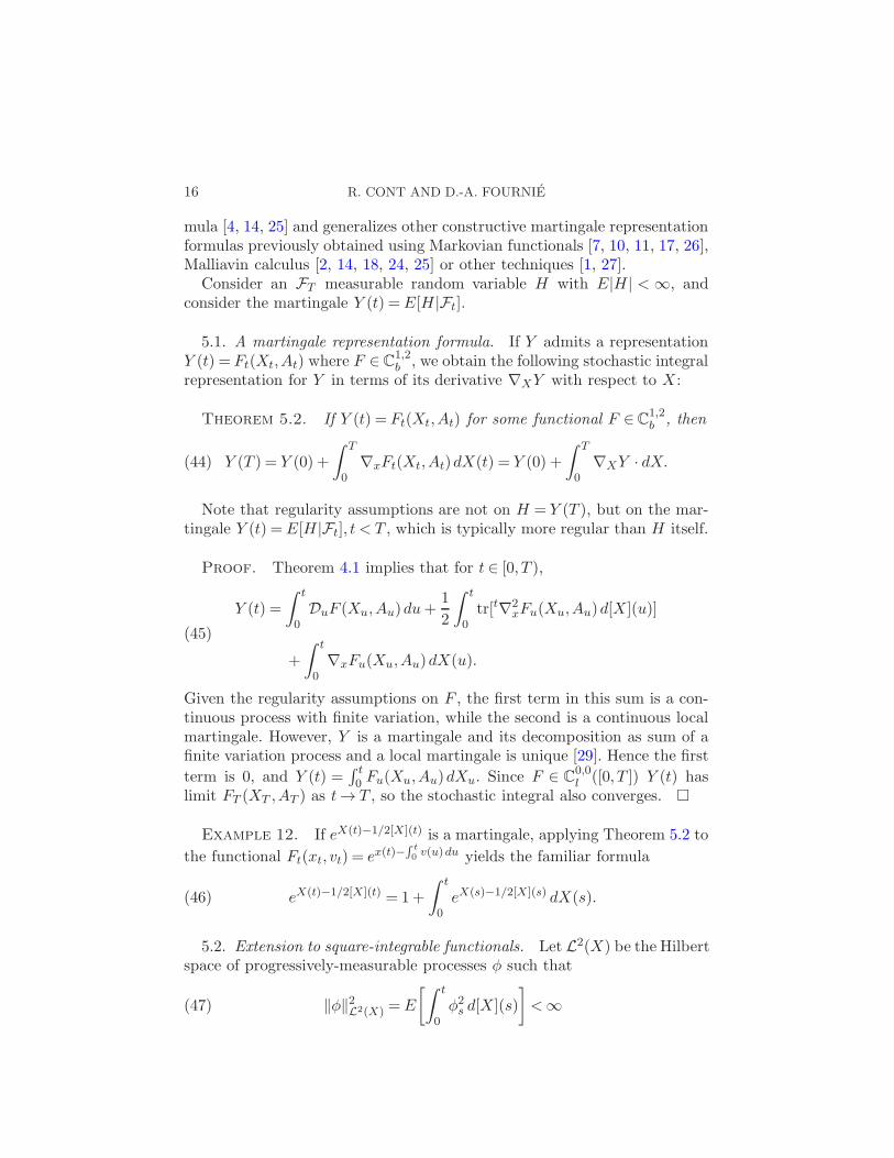
5.1. A martingale representation formula. If Y admits a representationY (t) = Ft(Xt,At) where F ∈C

1,2b , we obtain the following stochastic integral

representation for Y in terms of its derivative ∇XY with respect to X :

Theorem 5.2. If Y (t) = Ft(Xt,At) for some functional F ∈C1,2b , then

Y (T ) = Y (0) +

∫ T

0∇xFt(Xt,At)dX(t) = Y (0) +

∫ T

0∇XY · dX.(44)

Note that regularity assumptions are not on H = Y (T ), but on the mar-tingale Y (t) =E[H|Ft], t < T , which is typically more regular than H itself.

Proof. Theorem 4.1 implies that for t ∈ [0, T ),

Y (t) =

∫ t

0DuF (Xu,Au)du+

1

2

∫ t

0tr[t∇2

xFu(Xu,Au)d[X](u)]

(45)

+

∫ t

0∇xFu(Xu,Au)dX(u).

Given the regularity assumptions on F , the first term in this sum is a con-tinuous process with finite variation, while the second is a continuous localmartingale. However, Y is a martingale and its decomposition as sum of afinite variation process and a local martingale is unique [29]. Hence the first

term is 0, and Y (t) =∫ t0 Fu(Xu,Au)dXu. Since F ∈ C

0,0l ([0, T ]) Y (t) has

limit FT (XT ,AT ) as t→ T , so the stochastic integral also converges.

Example 12. If eX(t)−1/2[X](t) is a martingale, applying Theorem 5.2 to

the functional Ft(xt, vt) = ex(t)−∫ t

0 v(u)du yields the familiar formula

eX(t)−1/2[X](t) = 1+

∫ t

0eX(s)−1/2[X](s) dX(s).(46)

5.2. Extension to square-integrable functionals. Let L2(X) be the Hilbertspace of progressively-measurable processes φ such that

‖φ‖2L2(X) =E

[∫ t

0φ2s d[X](s)

]

<∞(47)


and I2(X) be the space of square-integrable stochastic integrals with respectto X .

I2(X) =

∫ .

0φ(t)dX(t), φ ∈L2(X)

(48)

endowed with the norm ‖Y ‖22 =E[Y (T )2]. The Ito integral IX :φ 7→∫ .0 φs dX(s)

is then a bijective isometry from L2(X) to I2(X).We will now show that the operator ∇X : 7→ L2(X) admits a suitable

extension to I2(X) which verifies

∀φ ∈ L2(X), ∇X

(∫

φ · dX

)

= φ, dt× dP-a.s.;(49)

that is, ∇X is the inverse of the Ito stochastic integral with respect to X .

Definition 5.3 (Space of test processes). The space of test processesD(X) is defined as

D(X) = C1,2b (X)∩ I2(X).(50)

Theorem 5.2 allows us to define intrinsically the vertical derivative of aprocess in D(X) as an element of L2(X).

Definition 5.4. Let Y ∈D(X) define the process ∇XY ∈ L2(X) as theequivalence class of ∇xFt(Xt,At), which does not depend on the choice ofthe representation functional Y (t) = Ft(Xt,At).

Proposition 5.5 (Integration by parts on D(X)). Let Y,Z ∈ D(X).Then

E[Y (T )Z(T )] =E

[∫ T

0∇XY (t)∇XZ(t)d[X](t)

]

.(51)

Proof. Let Y,Z ∈ D(X) ⊂ C1,2b (X). Then Y,Z are martingales with

Y (0) = Z(0) = 0 and E[|Y (T )|2]<∞,E[|Z(T )|2]<∞. Applying Theorem 5.2to Y and Z, we obtain

E[Y (T )Z(T )] =E

[∫ T

0∇XY dX

∫ T

0∇XZ dX

]

.

Applying the Ito isometry formula yields the result.

Using this result, we can extend the operator ∇X to define a weak deriva-tive on the space of (square-integrable) stochastic integrals, where ∇XY ischaracterized by (51) being satisfied against all test processes.


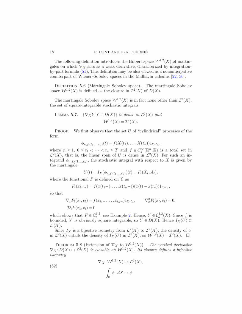
The following definition introduces the Hilbert space W1,2(X) of martin-gales on which ∇X acts as a weak derivative, characterized by integration-by-part formula (51). This definition may be also viewed as a nonanticipativecounterpart of Wiener–Sobolev spaces in the Malliavin calculus [22, 30].

Definition 5.6 (Martingale Sobolev space). The martingale Sobolevspace W1,2(X) is defined as the closure in I2(X) of D(X).

The martingale Sobolev space W1,2(X) is in fact none other than I2(X),the set of square-integrable stochastic integrals:

Lemma 5.7. ∇XY,Y ∈D(X) is dense in L2(X) and

W1,2(X) = I2(X).

Proof. We first observe that the set U of “cylindrical” processes of theform

φn,f,(t1,...,tn)(t) = f(X(t1), . . . ,X(tn))1t>tn ,

where n ≥ 1, 0 ≤ t1 < · · · < tn ≤ T and f ∈ C∞b (Rn,R) is a total set in

L2(X), that is, the linear span of U is dense in L2(X). For such an in-tegrand φn,f,(t1,...,tn), the stochastic integral with respect to X is given bythe martingale

Y (t) = IX(φn,f,(t1,...,tn))(t) = Ft(Xt,At),

where the functional F is defined on Υ as

Ft(xt, vt) = f(x(t1−), . . . , x(tn−))(x(t)− x(tn))1t>tn ,

so that

∇xFt(xt, vt) = f(xt1−, . . . , xtn−)1t>tn , ∇2xFt(xt, vt) = 0,

DtF (xt, vt) = 0

which shows that F ∈ C1,2b ; see Example 2. Hence, Y ∈ C1,2

b (X). Since f isbounded, Y is obviously square integrable, so Y ∈D(X). Hence IX(U) ⊂D(X).

Since IX is a bijective isometry from L2(X) to I2(X), the density of Uin L2(X) entails the density of IX(U) in I2(X), so W1,2(X) = I2(X).

Theorem 5.8 (Extension of ∇X to W1,2(X)). The vertical derivative∇X :D(X) 7→ L2(X) is closable on W1,2(X). Its closure defines a bijectiveisometry

∇X :W1,2(X) 7→ L2(X),(52)

∫ ·

0φ · dX 7→ φ


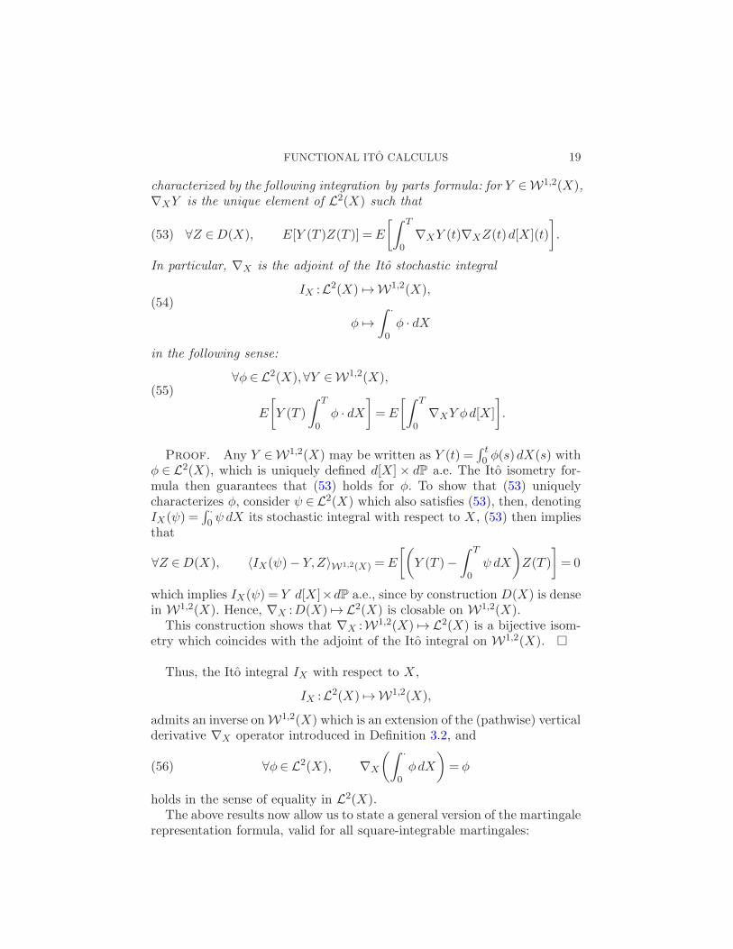
characterized by the following integration by parts formula: for Y ∈W1,2(X),∇XY is the unique element of L2(X) such that

∀Z ∈D(X), E[Y (T )Z(T )] =E

[∫ T

0∇XY (t)∇XZ(t)d[X](t)

]

.(53)

In particular, ∇X is the adjoint of the Ito stochastic integral

IX :L2(X) 7→W1,2(X),(54)

φ 7→

∫ ·

0φ · dX

in the following sense:

∀φ ∈L2(X),∀Y ∈W1,2(X),(55)

E

[

Y (T )

∫ T

0φ · dX

]

=E

[∫ T

0∇XY φd[X]

]

.

Proof. Any Y ∈W1,2(X) may be written as Y (t) =∫ t0 φ(s)dX(s) with

φ ∈ L2(X), which is uniquely defined d[X]× dP a.e. The Ito isometry for-mula then guarantees that (53) holds for φ. To show that (53) uniquelycharacterizes φ, consider ψ ∈L2(X) which also satisfies (53), then, denotingIX(ψ) =

∫ ·0 ψ dX its stochastic integral with respect to X , (53) then implies

that

∀Z ∈D(X), 〈IX(ψ)− Y,Z〉W1,2(X) =E

[(

Y (T )−

∫ T

0ψdX

)

Z(T )

]

= 0

which implies IX(ψ) = Y d[X]×dP a.e., since by construction D(X) is densein W1,2(X). Hence, ∇X :D(X) 7→ L2(X) is closable on W1,2(X).

This construction shows that ∇X :W1,2(X) 7→ L2(X) is a bijective isom-etry which coincides with the adjoint of the Ito integral on W1,2(X).

Thus, the Ito integral IX with respect to X ,

IX :L2(X) 7→W1,2(X),

admits an inverse onW1,2(X) which is an extension of the (pathwise) verticalderivative ∇X operator introduced in Definition 3.2, and

∀φ∈ L2(X), ∇X

(∫ ·

0φdX

)

= φ(56)

holds in the sense of equality in L2(X).The above results now allow us to state a general version of the martingale

representation formula, valid for all square-integrable martingales:


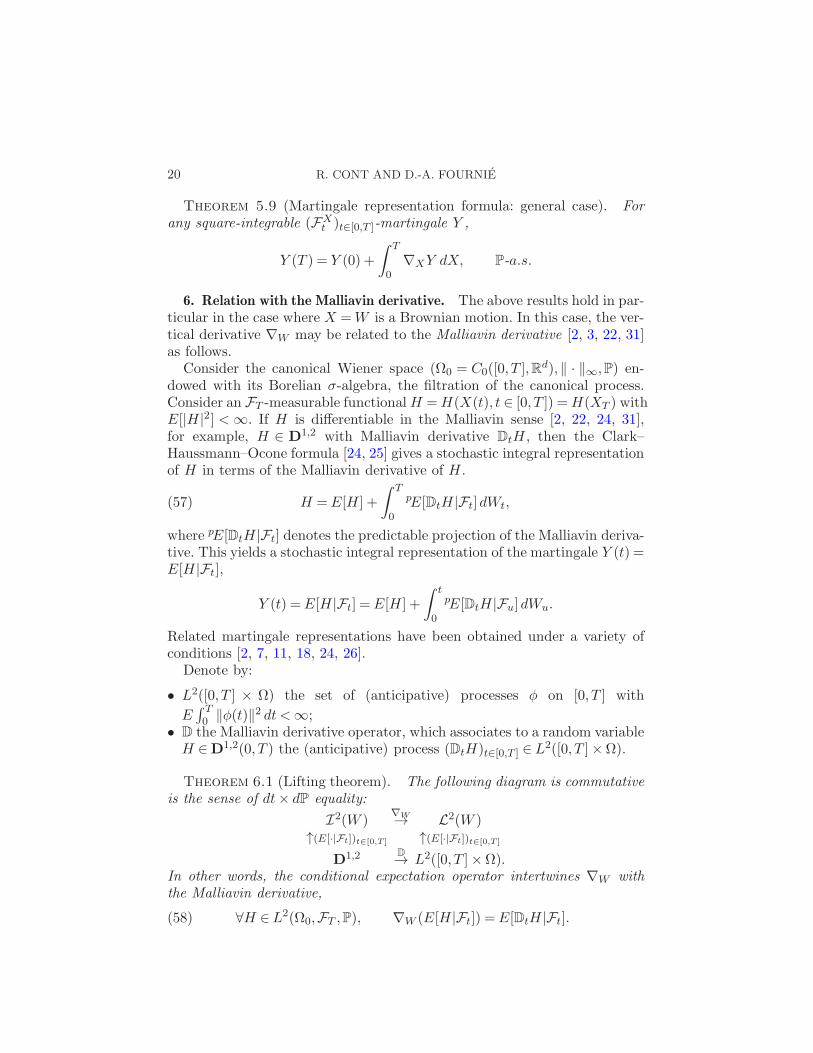
Theorem 5.9 (Martingale representation formula: general case). Forany square-integrable (FX

t )t∈[0,T ]-martingale Y ,

Y (T ) = Y (0) +

∫ T

0∇XY dX, P-a.s.

6. Relation with the Malliavin derivative. The above results hold in par-ticular in the case where X =W is a Brownian motion. In this case, the ver-tical derivative ∇W may be related to the Malliavin derivative [2, 3, 22, 31]as follows.

Consider the canonical Wiener space (Ω0 = C0([0, T ],Rd),‖ · ‖∞,P) en-

dowed with its Borelian σ-algebra, the filtration of the canonical process.Consider an FT -measurable functionalH =H(X(t), t ∈ [0, T ]) =H(XT ) withE[|H|2] <∞. If H is differentiable in the Malliavin sense [2, 22, 24, 31],for example, H ∈ D

1,2 with Malliavin derivative DtH , then the Clark–Haussmann–Ocone formula [24, 25] gives a stochastic integral representationof H in terms of the Malliavin derivative of H .

H =E[H] +

∫ T

0

pE[DtH|Ft]dWt,(57)

where pE[DtH|Ft] denotes the predictable projection of the Malliavin deriva-tive. This yields a stochastic integral representation of the martingale Y (t) =E[H|Ft],

Y (t) =E[H|Ft] =E[H] +

∫ t

0

pE[DtH|Fu]dWu.

Related martingale representations have been obtained under a variety ofconditions [2, 7, 11, 18, 24, 26].

Denote by:

• L2([0, T ] × Ω) the set of (anticipative) processes φ on [0, T ] with

E∫ T0 ‖φ(t)‖2 dt <∞;

• D the Malliavin derivative operator, which associates to a random variableH ∈D

1,2(0, T ) the (anticipative) process (DtH)t∈[0,T ] ∈ L2([0, T ]×Ω).

Theorem 6.1 (Lifting theorem). The following diagram is commutativeis the sense of dt× dP equality:

I2(W )∇W→ L2(W )

↑(E[·|Ft])t∈[0,T ] ↑(E[·|Ft])t∈[0,T ]

D1,2 D

→ L2([0, T ]×Ω).In other words, the conditional expectation operator intertwines ∇W withthe Malliavin derivative,

∀H ∈L2(Ω0,FT ,P), ∇W (E[H|Ft]) =E[DtH|Ft].(58)


Proof. The Clark–Haussmann–Ocone formula [25] gives

∀H ∈D1,2, H =E[H] +

∫ T

0

pE[DtH|Ft]dWt,(59)

where pE[DtH|Ft] denotes the predictable projection of the Malliavin deriva-tive. On other hand, Theorem 5.2 gives

∀H ∈ L2(Ω0,FT ,P), H =E[H] +

∫ T

0∇WY (t)dW (t),(60)

where Y (t) = E[H|Ft]. HencepE[DtH|Ft] = ∇WE[H|Ft], dt × dP almost

everywhere.

Thus, the conditional expectation operator (more precisely: the predictableprojection on Ft [8, Volume I]) can be viewed as a morphism which “lifts”relations obtained in the framework of Malliavin calculus into relations be-tween nonanticipative quantities, where the Malliavin derivative and theSkorokhod integral are replaced, respectively, by the vertical derivative ∇W

and the Ito stochastic integral.From a computational viewpoint, unlike the Clark–Haussmann–Ocone

representation which requires to simulate the anticipative process DtH andcompute conditional expectations, ∇XY only involves nonanticipative quan-tities which can be computed path by path. It is thus more amenable tonumerical computations. This topic is further explored in a forthcomingwork.

APPENDIX: PROOF OF THEOREM 2.7

In order to prove Theorem 2.7 in the general case where A is only requiredto be cadlag, we need the following three lemmas. The first lemma states aproperty analogous to “uniform continuity” for cadlag functions:

Lemma A.1. Let f be a cadlag function on [0, T ] and define ∆f(t) =f(t)− f(t−). Then

∀ε > 0,∃η(ε)> 0,(61)

|x− y| ≤ η ⇒ |f(x)− f(y)| ≤ ε+ supt∈(x,y]

|∆f(t)|.

Proof. If (61) does not hold, then there exists a sequence (xn, yn)n≥1

such that xn ≤ yn, yn−xn→ 0, but |f(xn)−f(yn)|> ε+supt∈[xn,yn]|∆f(t)|.We can extract a convergent subsequence (xψ(n)) such that xψ(n) → x. Not-ing that either an infinity of terms of the sequence are less than x or aninfinity are more than x, we can extract monotone subsequences (un, vn)n≥1

which converge to x. If (un), (vn) both converge to x from above or frombelow, |f(un) − f(vn)| → 0 which yields a contradiction. If one converges


from above and the other from below, supt∈[un,vn]|∆f(t)| ≥ |∆f(x)|, but|f(un)−f(vn)| → |∆f(x)|, which results in a contradiction as well. Therefore(61) must hold.

Lemma A.2. If α ∈R and V is an adapted cadlag process defined on afiltered probability space (Ω,F , (Ft)t≥0,P) and σ is a optional time, then

τ = inft > σ, |V (t)− V (t−)|> α(62)

is a stopping time.

Proof. We can write that

τ ≤ t=⋃

q∈Q∩[0,t)

(σ ≤ t− q ∩

supt∈(t−q,t]

|V (u)− V (u−)|> α

(63)

and, using Lemma A.1,

supu∈(t−q,t]

|V (u)− V (u−)|> α

(64)=

⋃

n0>1

⋂

n>n0

⋃

m≥1

sup1≤i≤2n

∣

∣

∣

∣

V

(

t− qi− 1

2n

)

− V

(

t− qi

2n

)∣

∣

∣

∣

>α+1

m

.

Lemma A.3 (Uniform approximation of cadlag functions by step func-tions). Let f ∈D([0, T ],Rd) and πn = (tni )n≥1,i=0,...,kn a sequence of parti-tions (0 = tn0 < t1 < · · ·< tnkn = T ) of [0, T ] such that

sup0≤i≤kn−1

|tni+1 − tni |n→∞→ 0, sup

u∈[0,T ]\πn

|∆f(u)|n→∞→ 0

then

supu∈[0,T ]

∣

∣

∣

∣

∣

f(u)−

kn−1∑

i=0

f(tni )1[tni ,tni+1)(u) + f(tnkn)1tnkn(u)

∣

∣

∣

∣

∣

n→∞→ 0.(65)

Proof. Denote hn = f −∑kn−1

i=0 f(tni )1[tni ,tni+1)+ f(tnkn)1tnkn. Since f −

hn is piecewise constant on πn and hn(tni ) = 0 by definition,

supt∈[0,T ]

|hn(t)|= supi=0,...,kn−1

sup[tni ,t

n+1i )

|hn(t)|= suptni <t<t

n+1i

|f(t)− f(tni )|.

Let ε > 0. For n ≥ N sufficiently large, supu∈[0,T ]\πn |∆f(u)| ≤ ε/2 andsupi |t

ni+1 − tni | ≤ η(ε/2) using the notation of Lemma A.1. Then, applying

Lemma A.1 to f we obtain, for n≥N ,

supt∈[tni ,t

n+1i )

|f(t)− f(tni )| ≤ε

2+ suptni <t<t

n+1i

|∆f(u)| ≤ ε.

We can now prove Theorem 2.7 in the case where A is a cadlag adaptedprocess.


Proof of Theorem 2.7. Let us first show that Ft(Xt,At) is adapted.Define

τN0 = 0, τNk = inf

t > τNk−1|2N t ∈N or |A(t)−A(t−)|>

1

N

∧ t.(66)

From lemma A.2, τNk are stopping times. Define the following piecewiseconstant approximations of Xt and At along the partition (τNk , k ≥ 0):

XN (s) =∑

k≥0

XτNk1[τN

k,τN

k+1[(s) +X(t)1t(s),

(67)AN (s) =

∑

k=0

AτNk1[τN

k,τN

k+1)(t) +A(t)1t(s),

as well as their truncations of rank K

KXN (s) =

K∑

k=0

XτNk1[τN

k,τN

k+1)(s), KA

N (t) =

K∑

k=0

AτNk1[τN

k,τN

k+1)(t).(68)

Since (KXNt ,K A

Nt ) coincides with (XN

t ,ANt ) for K sufficiently large,

Ft(XNt ,A

Nt ) = lim

K→∞Ft(KX

Nt ,K A

Nt ).(69)

The approximations Fnt (KXNt ,K A

Nt ) are Ft-measurable as they are contin-

uous functions of the random variables

(X(τNk )1τNk

≤t,A(τNk )1τN

k≤t), k ≤K,

so their limit Ft(XNt ,A

Nt ) is also Ft-measurable. Thanks to Lemma A.3, XN

t

and ANt converge uniformly to Xt and At, and hence Ft(XNt ,A

Nt ) converges

to Ft(Xt,At) since Ft : (D([0, t],Rd)×St,‖ · ‖∞)→R is continuous.To show the optionality of Z in point (ii), we will show that Z it as limit of

right-continuous adapted processes. For t ∈ [0, T ], define in(t) to be the inte-

ger such that t ∈ [ iTn ,(i+1)Tn ). Define the process Znt = F(in(t))T /n(X(in(t))T /n,

A(in(t))T /n), which is piecewise-constant and has right-continuous trajecto-

ries, and is also adapted by the first part of the theorem. Since F ∈ C0,0l ,

Zn(t)→ Z(t) almost surely, which proves that Z is optional. Point (iii) fol-lows from (i) and Lemma 2.6, since in both cases Ft(Xt,At) = Ft(Xt−,At−),and hence Z has left-continuous trajectories.

Acknowledgments. We thank Bruno Dupire for sharing his original ideaswith us, Hans-Jurgen Engelbert, Hans Follmer, Jean Jacod, Shigeo Kusuokaand an anonymous referee for helpful comments. R. Cont is especially grate-ful to the late Paul Malliavin for encouraging this work.


REFERENCES

[1] Ahn, H. (1997). Semimartingale integral representation. Ann. Probab. 25 997–1010.MR1434134

[2] Bismut, J.-M. (1981). A generalized formula of Ito and some other properties ofstochastic flows. Z. Wahrsch. Verw. Gebiete 55 331–350. MR0608026

[3] Bismut, J.-M. (1983). Calcul des variations stochastique et processus de sauts.Z. Wahrsch. Verw. Gebiete 63 147–235. MR0701527

[4] Clark, J. M. C. (1970). The representation of functionals of Brownian motion bystochastic integrals. Ann. Math. Statist. 41 1282–1295. MR0270448

[5] Cont, R. and Fournie, D. (2010). A functional extension of the Ito formula. C. R.Math. Acad. Sci. Paris 348 57–61. MR2586744

[6] Cont, R. and Fournie, D.-A. (2010). Change of variable formulas for nonanticipa-tive functionals on path space. J. Funct. Anal. 259 1043–1072. MR2652181

[7] Davis, M. H. A. (1980). Functionals of diffusion processes as stochastic integrals.Math. Proc. Cambridge Philos. Soc. 87 157–166. MR0549305

[8] Dellacherie, C. and Meyer, P.-A. (1978). Probabilities and Potential. North-Holland Mathematics Studies 29. North-Holland, Amsterdam. MR0521810

[9] Dupire, B. (2009). Functional Ito calculus. Portfolio Research Paper 2009-04,Bloomberg.

[10] Elliott, R. J. and Kohlmann, M. (1988). A short proof of a martingale represen-tation result. Statist. Probab. Lett. 6 327–329. MR0933291

[11] Fitzsimmons, P. J. and Rajeev, B. (2009). A new approach to the martingalerepresentation theorem. Stochastics 81 467–476. MR2569262

[12] Follmer, H. (1981). Calcul d’Ito sans probabilites. In Seminar on Probability, XV(Univ. Strasbourg, Strasbourg, 1979/1980) (French). Lecture Notes in Math. 850143–150. Springer, Berlin. MR0622559

[13] Haussmann, U. G. (1978). Functionals of Ito processes as stochastic integrals. SIAMJ. Control Optim. 16 252–269. MR0474497

[14] Haussmann, U. G. (1979). On the integral representation of functionals of Ito pro-cesses. Stochastics 3 17–27. MR0546697

[15] Ito, K. (1944). Stochastic integral. Proc. Imp. Acad. Tokyo 20 519–524. MR0014633[16] Ito, K. (1946). On stochastic differential equations. Proc. Imp. Acad. Tokyo 22 32–

35.[17] Jacod, J., Meleard, S. and Protter, P. (2000). Explicit form and robustness of

martingale representations. Ann. Probab. 28 1747–1780. MR1813842[18] Karatzas, I., Ocone, D. L. and Li, J. (1991). An extension of Clark’s formula.

Stochastics Stochastics Rep. 37 127–131. MR1148344[19] Kunita, H. and Watanabe, S. (1967). On square integrable martingales. Nagoya

Math. J. 30 209–245. MR0217856[20] Lyons, T. J. (1998). Differential equations driven by rough signals. Rev. Mat.

Iberoam. 14 215–310. MR1654527[21] Malliavin, P. (1978). Stochastic calculus of variation and hypoelliptic operators. In

Proceedings of the International Symposium on Stochastic Differential Equations(Res. Inst. Math. Sci., Kyoto Univ., Kyoto, 1976) 195–263. Wiley, New York.MR0536013

[22] Malliavin, P. (1997). Stochastic Analysis. Grundlehren der Mathematischen Wis-senschaften [Fundamental Principles of Mathematical Sciences] 313. Springer,Berlin. MR1450093

[23] Meyer, P. A. (1976). Un cours sur les integrales stochastiques. In Seminaire de Prob-abilites, X (Seconde Partie: Theorie des Integrales Stochastiques, Univ. Stras-

http://www.ams.org/mathscinet-getitem?mr=1434134





















bourg, Strasbourg, Annee Universitaire 1974/1975). Lecture Notes in Math. 511245–400. Springer, Berlin. MR0501332

[24] Nualart, D. (2009). Malliavin Calculus and Its Applications. CBMS Regional Con-ference Series in Mathematics 110. CBMS, Washington, DC. MR2498953

[25] Ocone, D. (1984). Malliavin’s calculus and stochastic integral representations offunctionals of diffusion processes. Stochastics 12 161–185. MR0749372

[26] Pardoux, E. and Peng, S. (1992). Backward stochastic differential equations andquasilinear parabolic partial differential equations. In Stochastic Partial Differ-ential Equations and Their Applications (Charlotte, NC, 1991). Lecture Notesin Control and Inform. Sci. 176 200–217. Springer, Berlin. MR1176785

[27] Picard, J. (2006). Brownian excursions, stochastic integrals, and representation ofWiener functionals. Electron. J. Probab. 11 199–248 (electronic). MR2217815

[28] Protter, P. E. (2005). Stochastic Integration and Differential Equations, 2nd ed.Stochastic Modelling and Applied Probability 21. Springer, Berlin. MR2273672

[29] Revuz, D. and Yor, M. (1999). Continuous Martingales and Brownian Motion, 3rded. Grundlehren der Mathematischen Wissenschaften [Fundamental Principlesof Mathematical Sciences] 293. Springer, Berlin. MR1725357

[30] Shigekawa, I. (1980). Derivatives of Wiener functionals and absolute continuity ofinduced measures. J. Math. Kyoto Univ. 20 263–289. MR0582167

[31] Stroock, D. W. (1981). The Malliavin calculus, a functional analytic approach.J. Funct. Anal. 44 212–257. MR0642917

[32] Watanabe, S. (1987). Analysis of Wiener functionals (Malliavin calculus) and itsapplications to heat kernels. Ann. Probab. 15 1–39. MR0877589

Laboratoire de Probabilites et Modeles Aleeatoires

CNRS—Universite Pierre & Marie Curie

4 place Jussieu, Case Courrier 188

75252 Paris

France

E-mail: [email protected]

Department of Mathematics

Columbia University

New York, New York 10027

USA

E-mail: [email protected]











mailto:[email protected]

mailto:[email protected]

Documents

Functional It calculus and stochastic integral ...2013, Vol. 41, No. 1, 109–133 DOI: 10.1214/11-AOP721 c Institute of Mathematical Statistics, 2013 FUNCTIONAL ITO CALCULUS AND ... ·