Functional Data Analysis in Brain ImagingStudies

Tian Siva Tian ∗

Abstract

Functional data analysis (FDA) considers the continuity of the curves orfunctions, and is a topic of increasing interest in the statistics community.FDA is commonly applied to time-series and spatial-series studies. The de-velopment of functional brain imaging techniques in recent years made itpossible to study the relationship between brain and mind over time. Con-sequently, an enormous amount of functional data is collected and needs tobe analyzed. Functional techniques designed for these data are in strong de-mand. This paper discusses three statistically challenging problems utilizingFDA techniques in functional brain imaging analysis. These problems aredimension reduction (or feature extraction), spatial classification in fMRIstudies, and the inverse problem in MEG studies. The application of FDAto these issues is relatively new but has been shown to be considerably ef-fective. Future efforts can further explore the potential of FDA in functionalbrain imaging studies.

Keywords: Functional data analysis; Brain imaging; Dimension reduction; Spatialclassification; Inverse problem.

1 IntroductionFunctional data refer to curves or functions, i.e. the data for each variable areviewed as smooth curves, surfaces, or hypersurfaces evaluated at a finite subsetof some interval (e.g., some period of time, some range of temperature and so

∗Department of Psychology, University of Houston, Houston, TX 77204. Email:ttian@uh.edu.

1

on). Functional data are intrinsically infinite-dimensional but are usually mea-sured discretely. Statistical methods for analyzing such data are described by theterm “functional data analysis” (FDA) coined by Ramsay and Dalzell (1991). Dif-ferent from multivariate data analysis, FDA considers the continuity of the curvesand models the data in the functional space rather than treating them as a set ofvectors. Ramsay and Silverman (2005) give a comprehensive overview of FDA.

Among many of the most popular FDA applications, functional neuroimag-ing has created revolutionary movements in medicine and neuroscience. Modernfunctional brain imaging techniques, such as PET (positron emission tomogra-phy), fMRI (functional magnetic resonance imaging), EEG (electro-encephalography)and MEG (magneto-encephalography), have been used for assessing the func-tional organization of the human/animal brain. These techniques allow real-timeobservation of the underlying brain processes during different experimental condi-tions, and have emerged as a crucial tool to understand and to assess new therapiesfor neurological disorders. These techniques measure different aspects of brainactivity at some discrete time points during an experiment using different prin-ciples. These measurements, called time courses, can be treated as functions oftime. Methods designed to characterize the functional nature of the time coursesare in strong demand.

In this paper, we present three problems in brain imaging studies. Not onlyFDA has already drawn a great deal of attention and become more and more im-portant in these problems, but also data analysis in these problems is difficult.First, a brain imaging experiment usually lasts several minutes long and the sig-nal amplitudes are recorded every 1-2 seconds. Normally the total number of timepoints can be 200-1000. In addition, there could be hundreds or even thousands ofsuch time courses. Let us take fMRI as an example. As mentioned earlier, fMRIrecords the hemodynamic response in the brain that signals neural activity withhigh spatial resolution. It records signals at the millimeter scale (2-3mm is typicaland sometimes can be as good as 1mm). These small elements of a 3-dimensionalbrain image are cubic volumes and are called “voxels”, which is an extension ofthe term “pixel” in a 2-dimensional image. There can be thousands of thousandssuch voxels in a 3-D brain image. Figure 1 shows an example of fMRI scan at onetime point (from http://www.egr.vcu.edu/cs/Najarian_Lab/fmri.html).The activity level (signal amplitude) is represented by different colors (see thelower right panel for a reference). The dark red areas are the most active areas;the light yellow areas are less active; and the gray areas have very low activity.Note that the signal amplitude at each voxel is recorded over time, so we willhave many images as Figure 1. Therefore, the data volume can be huge. The

2

Figure 1: An example fMRI scan showing brain activity.

enormous amount of data render many standard techniques impractical.Second, although time courses are considered continuous, current functional

brain imaging devices can only record the brain activity changes discretely. Inother words, they measure signal amplitudes at a sample of time points, whichis usually evenly spaced (e.g., every 1-2 seconds). This temporal sampling isrelatively sparse, because brain waves for some specific tasks change fast. Forexample, when studying auditory brainstem, the stimuli are usually brief (e.g.,about 100 ms) with several cycles (Roberts and Poeppel, 1996). The change ofbrain waves is also fast, because the response functions in the brain are highlycorrelated with the stimuli. The sparse sampling can hardly capture some charac-teristics of the brain activity.

Third, the hypotheses on how the brain activates are sometimes difficult toformalize. In some cases, the reference function can be used to formulate the

3

hypothesis, but it is not always the case. In many studies there is no such ref-erence function (e.g., decision making, reasoning and emotional processes). Inthese studies, formulating the hypothetical brain wave has to borrow ideas frommany disciplines, including cognitive neuroscience, social psychology, neuropsy-chology and so on.

The rest of the paper is constructed as follows. In Sections 2, 3, and 4, wepresent three of the issues in brain imaging studies: dimension reduction, spatialclassification, and the inverse problem. In each section, we compare differentcommonly used multivariate and functional methods, and our results show thatusing FDA can lead to better results in general. The data sets used in this paperare from an fMRI vision study and an MEG somatosensory study.

2 Dimension ReductionFunctional data is intrinsically infinite dimensional. Even though they are mea-sured discretely over a finite set of some interval, the dimensionality (i.e., thenumber of measurements) is high. This introduces the “curse of dimensionality”(Bellman, 1957) and causes problems with data analysis (Aggarwal et al., 2001).High-dimensional data significantly slow down conventional statistical algorithmsor even make them practically infeasible. For example, one may wish to classifytime courses into different groups. Standard classification methods may sufferfrom difficulties of handling the entire time courses when the dimension is high.Even if some advanced techniques can be applied to the entire time courses (e.g.support vector machines and neural networks), classification accuracy and com-putation cost can be significantly improved by using a small subset of “important”measurements or a handful of components that combine in different ways to rep-resent features of the time courses. One reason is that consecutive time points areusually highly correlated, including too much redundancy may increase the noiselevel and hence mask useful information about the true structure of the data.

In addition, it is usually not necessary to manipulate the entire time course. Forthe purpose of model interpretation, using a small number of the most informativefeatures may help build a relatively simpler model and reveal the underlying datastructure. Hence, one can better explain the relationship between the input andoutput of the model.

Therefore, dimension reduction (or feature extraction) should be applied tocompress the time courses, keeping only relevant information and removing cor-relations. This procedure will not only speed up but also improve the accuracy of

4

the follow-up analyses. Furthermore, the model may be more interpretable whenonly a handful of important features are involved.

Let xi(t) be the ith time course, i= 1,2, . . . ,N, where ti ∈Ti = ti,1, ti,2, . . . , ti,M..For notational simplicity, we assume that the Ti’s are the same for all N timecourses. Hence, we denote T = t1, t2, . . . , tM for all xi(t)’s. Suppose that thereduced data are stored in a matrix, Z ∈ RN×K , where each row represents a timecourse and each column represents a feature in a new coordinate system.

Generally, dimension reduction for functional data can be expressed as

zi,k =∫

xi(t) fk(t)dt, i = 1, . . . ,N, k = 1, . . . ,K, (1)

where zi,k is the (i,k)th element in the reduced data (feature space) Z and fk(t) issome so-called transformation function that transforms xi(t)’s to the new coordi-nate system.

In the following subsections, we briefly describe three popular dimension re-duction approaches that are widely applied to functional neuroimaging studies.

2.1 FPCAFunctional principal component analysis (FPCA) is an extension of multivariatePCA and was an critical part of FDA in early work. In the context of brain imagingstudies, it is especially useful when there is uncertainty as to the duration of amental state induced by an experimental stimulus, e.g., a decision making processor an emotional reaction. This is because as an explorative technique, FPCA doesnot make assumptions on the form of brain waves. A few studies have includedFPCA. Viviani et al. (2005) used FPCA to single subject to extract the featuresof hemodynamic response in fMRI studies, and showed that FPCA outperformedmultivariate PCA. Long et al. (2005) used FPCA on multiple subjects to estimatethe subject-wise spatially varying non-stationary noise covariance kernel.

As with multivariate PCA, FPCA explores the variance-covariance and thecorrelation structure. It identifies functional principal components that explainthe most variability of a set of curves by calculating the eigenfunctions of theempirical covariance operator. FPCA also can be expressed using Equation (1), inwitch the transformation functions, fk(t)’s are orthonormal eigenfunctions. Thatis, ∫

f j(t) fk(t)dt =

0 j 6= k1 j = k

5

In the matrix form, Equation (1) can be expressed as

zi,k = fTk xi, (2)

where elements in fk and xi are realizations of the kth eigenfunction and the ithobserved time course, respectively.

There are several issues when applying FPCA. One is to choose the form ofthe orthonormal eigenfunctions. Note that any functions can be represented by itsorthogonal bases. The choice of the basis decides the shape of the curve. Usually,the bases should be chosen such that the expansion of each curve in terms ofthese basis functions approximates the curve as closely as possible (Ramsay andSilverman, 2005). That is,

min∫

[xi(t)− xi(t)]2 dt,

where xi(t) = ∑Kk=1 zi,k fk(t). Ramsay and Silverman (2005) give a detailed expla-

nation of how to solve for fk(t).Another issue is to choose the number of eigenfunctions, K. This is an im-

portant practical issue without a satisfactory theoretical solution. Presumably, thelarger the K, the more flexible the approximation would be, and hence, the closerto the true curve. However, a large K always results in a complex model whichintroduces difficulties to follow-up analyses. In addition, interpreting a large num-ber of of the orthogonal components may be difficult. One wishes every eigen-function can capture a meaningful feature of the curves so that the componentscan be interpretable. Simpler models with fewer components are considered moreinterpretable and hence are more preferable. However, this is not always straight-forward in real life. The most commonly used approach to choose K is estimatingthe number of components based on the estimated explained variance (Di et al.,2009).

2.2 Filtering MethodsAnother type of approaches that conduct dimension reduction is the so-called fil-tering methods, which approximate each function by a linear combination of afinite number of basis functions and represent the reduced data by the resultingbasis coefficients. Since measurement errors may come along with the data, theobserved curves may contain roughness. Filtering methods are put forth to smooth

6

the curve. One can use a K-dimensional basis function to transform xi(t)’s intonew features. We write

xi(t) =K

∑k=1

bk(t)θi,k = b(t)Tθθθ i, (3)

where b(t) = [b1(t),b2(t), . . . ,bK(t)]T is a K-dimensional basis function and θθθ i =[θi,1,θi,2, . . . ,θi,K]

T is the corresponding coefficient vector of length K. The coef-ficients θθθ i’s are usually treated as the extracted features. The θθθ i’s can be estimatedby using the least squares solution:

θθθ i = (BT B)−1BT xi = Sxi, (4)

where B is defined as the m-by-K matrix containing the values of bk(t j)’s, S =(BT B)−1BT and xi’s are the observed measurements of the ith functional curve attime points T . Hence we have

θi,k = sTk xi, (5)

where sk, k = 1,2, . . . ,K is the jth row of S and θi,k is the kth estimated coefficientof θθθ i. This way a filtering method can also be represented using the same form ofEquation (1). The θi,k is equivalent to zi,k and sk is equivalent to the realizationsof fk at time points T .

One issue with the filtering methods is the selection of basis functions. Com-monly used techniques use the Fourier or the wavelet bases to project the signalinto the frequency domain or a tiling of the time-frequency plane, respectively.By keeping the first K coefficients as features, each time course is represented bya rough approximation. This is because these coefficients correspond to the lowfrequencies of the signal, where most signal information is located. Alternatively,one can also use the K largest coefficients instead, because these coefficients pre-serve the optimal amount of energy present in the original signal (Wu et al., 2000).Criteria for choosing K is similar to choosing K eigenfunctions in FPCA.

2.3 A Classification Oriented MethodOne alternative to the aforementioned methods is the FAC method proposed byTian and James (2010). FAC deals with functional dimension reduction prob-lems for classification tasks specifically. This method is highly interpretable andhas been demonstrated effective in different classification scenarios. Similarly

7

to FPCA and filtering methods, FAC also follows Equation (1) and finds a set offk(t)’s so that the transformed multivariate data Z can be optimally classified. Theidea of FAC is expressed as follows

F(t) = argminF(t)Ex(t),Y [e(MF(t)(x(t)),Y )], (6)subject to some γ(F)≤ λ .

where scalar Y is the group label, F(t) = [ f1(t), f2(t), . . . , fK(t)]T , MF(t) is a pre-selected classification model applied to the lower-dimensional data, e is a lossfunction resulting from MF(t), and γ(F) constrains the model complexity. Byadding this constraint, the solution to Equation (6) can achieve better interpretabil-ity. In practice, this constraint can be set to constrain the shape of f j(t)’s. Forexample, one can let the f j(t) be piecewise constant or piecewise linear. Thesesimple structures are considered more interpretable than structures involving morecurvature.

Equation (6) is a difficult non-linear optimization problem and is hard to solve.Tian and James (2010) proposed a stochastic search procedure guided by the eval-uation of model complexity. This procedure makes use of the group informationand produces simple relationships between the reduced data and the original func-tional predictor. Therefore, this dimension reduction method is particularly usefulwhen dealing with classification problems (see Section 3).

The aforementioned functional methods assume that xi(t)’s are fixed unknownfunctions. When the noise level is high (e.g., single-trial EEG/MEG), it is difficultto represent the time course properly with a basis expansion having deterministiccoefficients. A stochastic representation such as the well-localized wavelet basis(Nason et al., 1999) or the smooth localized Fourier basis (Ombao et al., 2005)may be more preferable.

In many circumstances, the aforementioned dimension reduction methods canefficiently reduce the data dimension and significantly speed up the follow-upanalyses. The choice of a dimension reduction method should be guided by thefollow-up analyses. For example, if the final goal is extracting orthogonalizedlower dimensional features and there is uncertainty of the mental state, then FPCAmay be a better choice. If the goal is further analyzing the data features or fea-ture selections, then filtering methods may be a good option. This is becausea filtering method can be performed in the frequency domain. One then selectslow frequency features which contain most signal information. If the final goal isclassifying different sets of functions, then FAC may dominate others.

8

2.4 An ExampleIn this section, we demonstrate the effectiveness of the aforementioned dimensionreduction approaches on a classification task in an fMRI study. Since the goalis classification, we expect that the classification oriented FAC method wouldoutperform others in terms of classification accuracy. The idea is to reduce thedimension of the time courses first and then utilize the reduced data as the inputof a classification model.

The data set came from a vision study that were conducted in the ImagineCenter at the University of Southern California. There are five main subareas inthe visual cortex of the brain: the primary visual cortex (striate cortex or V1) andthe extrastriate visual cortical areas (V2, V3, V4, and V5). Among them, theprimary visual cortex is highly specialized for mapping the spatial informationin vision, that is, processing information about static and moving objects. Theextrastriate visual cortical areas are used to distinguish fine details of the objects.The main goal for this study is to identify subareas V1 and V3. Presumably,voxel amplitude time courses in the V1 area are different from time courses inthe V3 area. Since the boundaries for these two subareas are relatively clear, it isreasonable to utilize these data to evaluate the performance of the aforementioneddimension reduction methods in classification.

The data contain 6924 time courses, where 2058 are from V1 and 4866 arefrom V3. These time courses are measured at 404 time points. These 404 mea-surements are averages of three trails. We sample 600 time courses, evenly spaced,from V1. Then we randomly select 500 time courses and put them in the trainingdata, and the rest 100 are placed into the test data. We do the same process toV3 and obtain 500 training time courses and 100 test time courses. Hence, thetotal training and test data contain 1000 and 200 time courses, respectively. Weapply FPCA, filtering methods, and FAC to reduce the dimensionality of the data.For filtering methods, we examine B-Spline bases (Filtering1) and Fourier Bases(Filtering2). For FAC, we examine the piecewise constant version (FAC1) and thepiecewise linear version (FAC2). That is, FAC1 constrains f j(t)’s to be piecewiseconstant and FAC2 constrains f j(t)’s to be piecewise linear. The final classifieris an standard logistic regression. Note that other classifiers can be applied, butwe use logistic regression as an example, since the goal is to evaluate dimensionreduction methods given a fixed classifier. Tian and James (2010) have comparedfiltering methods with FAC in the same setting. Here we extend the comparisonsto FPCA. We examine when K = 4 and 10. That is, reduce the data to either 4 or10 dimensions, then apply a logistic regression to the lower dimensional data. Ta-

9

ble 1 shows test misclassification rates on the reduced data. The misclassificationrate is defined as the ratio of the number of misclassified test time courses to thetotal number of test time courses. Note that other criteria can be used to evaluateclassification accuracy. Since FAC is a stochastic search based method, we applyit 10 times (with each time 100 iterations) on these data and compute the averagetest misclassification rate and the standard error (in the parentheses).

As expected, both versions of FAC outperform other methods in general. Inparticular, FAC2 provides the best accuracy. Between the other two methods,when K is small FPCA seem to work better than filtering methods, but when K islarge filtering methods show slight advantages over FPCA.

Table 1: Misclassification rates on the reduced data (classifier: logistic regres-sion).

FPCA Filtering1 Filtering2 FAC1 FAC2K = 4 0.287 0.385 0.360 0.100(0.003) 0.096(0.004)K = 10 0.112 0.091 0.105 0.056(0.004) 0.050(0.004)

One problem with FAC is that it is a stochastic search based method, there-fore, the computation cost is more than the the other two deterministic methods.We investigate the computation time of these three methods. All methods are im-plemented in R and run on a 64-bit Dell Precision workstation (CPU 3.20GHz;RAM 24.0GB). For FAC1, we examine one run with 100 iterations. We recordedthe total CPU time (in seconds) of the R program and list it in Table 2. As we cansee, the computation cost for FAC is much higher than that for FPCA and filteringmethods, even though its accuracy is high.

Table 2: Execution time in second.

FPCA Filtering1 FAC1K = 4 4.67 3.12 78.18K = 10 8.24 5.25 129.56

Again, there is not a universal dimension reduction method. This example onlyshows the performance of different methods when the final goal is classification.There may be the case that FAC is less preferable when the goal is, say extractinglow frequency features. One need to choose an appropriate method based on theultimate goal. Also, computation cost is another factor that needs to be considered.One should seek for a balance between accuracy and cost.

10

3 Spatial Classification Problems in fMRIThe high spatial resolution of fMRI enables us to obtain more precise and betterlocalized information. Therefore, it is usually used to analyze neural dynamics atdifferent functional regions in the brain. However, it is difficult to identify somesmall functional sub-areas for a specific task. One commonly used method isbased on theories in neurobiology and cognitive sciences. This is to assume thatdifferent functional sub-areas have different neural dynamic responses (i.e., voxelamplitude functions are different in different sub-areas) given a specific task. Letus use the visual example again. Based on the visual transmission theories, thevisual information is carried out through neural pathways from V1 to V5. Theinformation first reaches the V1 area and then V2 and so on. The neural responsefunctions in these sub-areas differ in terms of the amplitudes and frequencies.Therefore, by comparing the shape of the neural response functions in differentsub-areas, these visual cortical sub-areas can be identified. In many fMRI studiesso far, this comparison is mostly done by naked eye, which is inefficient andinaccurate. In addition, since, for example, the visual transmission is a non-linearcontinuous process (Zhang et al., 2006), there is no a clear boundary betweentwo adjacent sub-areas. The characteristics for voxels near the boundary might bevery similar. This results in large within-group variations and, hence, the naked-eye method is unsatisfactory.

Two commonly used techniques for spatial classification are machine learningmethods and functional discriminant methods.

3.1 Machine Learning MethodsMachine learning methods are applied in two ways. One way is discard temporalorders and treat the time courses as multivariate vectors. Then one can applyclassification techniques to these “vectors” directly. To implement, one obtains thedata consisting of the neural dynamic response functions and their correspondingclass labels. These data should be selected from the region where the class labelsare relatively clear, e.g., the center of an sub-area. These data are divided intotraining and test sets. The training data are used to fit the model and select tuningparameters for the model, and the test data are used to examine the performanceof the fitted model. Once the model is built, it can be applied to new data wherethe group labels are unknown.

Since the dimension of the vectors (i.e., the number of measurements in thetime courses) can be a few hundred, many standard multivariate classification

11

methods are unsatisfactory. There are some advanced methods designed for high-dimensional data such as support vector machines (SVM) (Vapnik, 1998), treed-based methods (Breiman, 2001; Tibshirani and Hastie, 2007), and neural networks(NN) (HERTZ et al., 1991). These methods can be applied to handle time coursesclassification. However, these methods do not consider the functional nature ofthe time courses and thus have disadvantages. As mentioned earlier, adjacentmeasurements in a time course are highly correlated. In addition, time courses infunctional brain imaging studies contain a lot of noise and important classificationinformation usually lies in small portions of the time courses, e.g., some peakareas. Therefore, it is not necessary to include all measurements in the model.

Another way consists of two parts: dimension reduction and classification.More specifically, first reduce the data dimension and then apply classificationtechniques to the reduced data. For We have discussed some methods for dimen-sion reduction in Section 2. These methods transform the data onto a new featurecoordinate system and select a handful of important features in this new coordi-nate system. Another type of dimension reduction is selecting a subset of relevantmeasurements from the entire time courses instead of transforming the data. Thiscan be done through a variable selection technique, such as the Lasso (Efron et al.,2004; Tibshirani, 1996), SCAD (Fan and Li, 2001), nearest shrunken centroids(Tibshirani et al., 2002), the Elastic Net (Zou and Hastie, 2005), Dantzig selector(Candes and Tao, 2007), VISA (Radchenko and James, 2008) and FLASH (Rad-chenko and James, 2010). Then a standard classification classification techniquecan be applied to the selected measurements.

3.2 Functional Discriminant MethodsFunctional discriminant methods have also been studied. These methods considerthe functional nature of the time courses. In general, the idea can be viewedas extensions of classical statistics to the functional space. One extension is thegeneralized linear model in the functional form, i.e., the functional regressionmodel with a scalar response and a functional predictor. Let Y be the categoricalresponse variable. Consider the model

yi = β0 +∫

β (t)xi(t)dt + ei, i = 1,2, . . . ,N, (7)

where yi is the class label for the ith time course and the unknown functionalcoefficient β (·) measures the dependence of yi on xi. Note that xi(t) is the “true”

12

underlying function for the ith time course and it is unobserved. The measurementxi, j is the perturbed value of xi(t) at time t j and the perturbation is ei.

To solve Equation (7), many methods were proposed. Some examples are thegeneralized singular value decomposition method (Alter et al., 2000), the lineardiscriminant method for sparse functional data (James and Hastie, 2001), the para-metric method with the generalized linear model involved (James, 2002; Muller,2005; Muller and Stadtmuller, 2005), nonparametric methods (Ferraty and Vieu,2003; Hall et al., 2001), the smoothing penalization method (Ramsay and Silver-man, 2005), the factorial method of testing various sets of curves (Ferraty et al.,2007), and the robust method with estimation of the data depth (Cuevas et al.,2007).

Many of the aforementioned methods involve a dimension reduction step aswell. For example, Alter et al. (2000), Hall et al. (2001), and Muller (2005);Muller and Stadtmuller (2005) used the Karhunen-Loeve decomposition to trans-form the covariance function to a diagonalized space. James (2002); James andHastie (2001) used filtering methods to approximate xi(t)’s and β (t), i.e., usingcoefficients of basis functions instead of the original measurements. We describethree methods below.

James (2002) used natural cubic spline (NCS) bases to expand xi, j’s and ap-proximate the β (t).

xi, j =K

∑k=1

zi,kφk(t j)+ εi, j = φφφ(t j)T zi + εi, j, (8)

β (t) =L

∑l=1

clψl(t) = cTψψψ(t), (9)

where φφφ is a K-dimensional NCS basis, zi is its corresponding coefficient vector,and ψψψ is a L-dimensional NCS basis. Equation (8) expands the (i, j)th measure-ment by its basis functions. Equation (9) approximates β (t) by its basis. Thecoefficient vector c can be estimated using the maximum likelihood method.

Muller (2005) used the Karhunen-Loeve decomposition to decompose xi(t)’sto a diagonalized space. In this case, Equation (3) is used to approximate xi(t)’s,b(t) contains the first K eigenfunctions of xi(t)’s and θi,k’s are all uncorrelated,i.e., the variance-covariance matrix is diagonal. Then Equation (7) can be writtenas

yi = β0 +∫

β (t)

[K

∑k=1

bk(t)θi,k

]dt = β0 +

K

∑k=1

θi,k

∫β (t)bk(t)dt. (10)

13

Let ηk =∫

β (t)bk(t)dt. Then ηk’s can be estimated by regressing yi on θi,1, . . . ,θi,K

yi = β0 +K

∑k=1

bk(t)θi,k.

Hence, this method is a two-step approach. The first step is dimension reduction,then the second step is classification.

Ramsay and Silverman (2005) approximated xi(t) and β (t) using Equations(3) and (9), respectively, with a large number of bases for xi(t)’s. We write

X(t) = Θb(t)

where the coefficient matrix Θ is N-by-K. Then Equation (7) becomes

yi = β0 +∫

Θb(t)ψψψ(t)T c = ΘΩc, (11)

where X(t) = [x1(t), . . . ,xN(t)]T , Ω =∫

b(t)ψψψ(t)T dt is a K-by-L matrix. Thenβ (t) can be estimated by minimizing a penalized residual sum of squares

minβ (t)

N

∑i=1

[yi−β0−

∫β (t)xi(t)dt

]2

+λ

∫[Lβ (t)]2dt

, (12)

where λ is some smoothing parameter and L is a linear differential operator.As mentioned earlier, one potential limitation of the aforementioned func-

tional methods is that when the noise level in the observed time courses is high.These data cannot be adequately represented by FDA when the coefficients areassumed fixed but unknown. Stochastic coefficient methods (Nason et al., 1999;Ombao et al., 2005) may provide better solutions. For example, (Ho et al., 2008)utilized the Ombao et al. (2005)’s method to capture the transient features of brainsignals in the frequency domain, then used relevant time-frequency features todistinguish between groups.

3.3 An ExampleIn this section, we examine the performance of four methods on a spatial classi-fication task. The four methods include three machine learning methods and onefunctional discriminant method. First, we apply SVM directly to the entire timecourses treating them as multivariate vectors. Second, we apply a filtering method

14

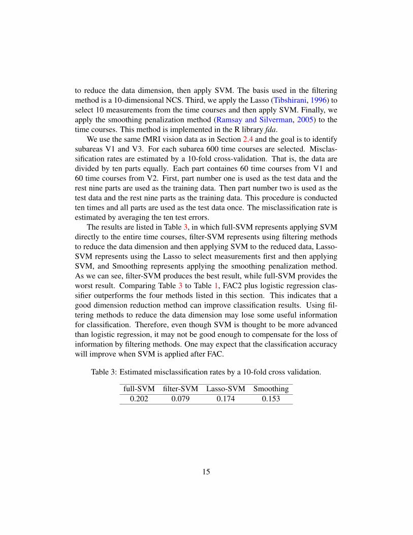
to reduce the data dimension, then apply SVM. The basis used in the filteringmethod is a 10-dimensional NCS. Third, we apply the Lasso (Tibshirani, 1996) toselect 10 measurements from the time courses and then apply SVM. Finally, weapply the smoothing penalization method (Ramsay and Silverman, 2005) to thetime courses. This method is implemented in the R library fda.

We use the same fMRI vision data as in Section 2.4 and the goal is to identifysubareas V1 and V3. For each subarea 600 time courses are selected. Misclas-sification rates are estimated by a 10-fold cross-validation. That is, the data aredivided by ten parts equally. Each part containes 60 time courses from V1 and60 time courses from V2. First, part number one is used as the test data and therest nine parts are used as the training data. Then part number two is used as thetest data and the rest nine parts as the training data. This procedure is conductedten times and all parts are used as the test data once. The misclassification rate isestimated by averaging the ten test errors.

The results are listed in Table 3, in which full-SVM represents applying SVMdirectly to the entire time courses, filter-SVM represents using filtering methodsto reduce the data dimension and then applying SVM to the reduced data, Lasso-SVM represents using the Lasso to select measurements first and then applyingSVM, and Smoothing represents applying the smoothing penalization method.As we can see, filter-SVM produces the best result, while full-SVM provides theworst result. Comparing Table 3 to Table 1, FAC2 plus logistic regression clas-sifier outperforms the four methods listed in this section. This indicates that agood dimension reduction method can improve classification results. Using fil-tering methods to reduce the data dimension may lose some useful informationfor classification. Therefore, even though SVM is thought to be more advancedthan logistic regression, it may not be good enough to compensate for the loss ofinformation by filtering methods. One may expect that the classification accuracywill improve when SVM is applied after FAC.

Table 3: Estimated misclassification rates by a 10-fold cross validation.

full-SVM filter-SVM Lasso-SVM Smoothing0.202 0.079 0.174 0.153

15

4 The Inverse Problem in MEGMEG is a noninvasive powerful technique that can track the magnetic field accom-panying synchronous neuronal activities with temporal resolution easily reachingmillisecond level. Therefore, it is able to capture the rapid change in corticalactivity. With recent development of whole-head biomagnetometer systems thatprovide high spatial resolution in magnetic field coverage, MEG possesses uniquecapability to localize the detected neuronal activities and follow its changes mil-lisecond by millisecond when suitable source modeling techniques are utilized.Thus it is attractive in cognitive studies of normal subjects and in neurological orneurosurgical evaluation of patients with brain diseases. In MEG studies, evokedresponses are measured over time by a set of sensors outside the head of a patient.One of the issues is reconstructing and localizing the signal sources of evokedevents of interest in the brain based on the measured MEG time courses. This isthe so-called “inverse problem”.

For example, in a somatosensory experiment, data were recorded by an MEGdevice with 247 sensors (channels). Each sensor records 228 measurements dur-ing one trail. One then averages all three trails. Figure 2 shows the time coursesfrom the 247 channels (left panel) and their corresponding isofield magnetic maps(right panel), respectively. Stimuli were presented at time points 85 and 99. As wecan see from the left panel of Figure 2, the evoked activity time courses achievethe peaks at 85 and 99. We expect that the reconstructed source time coursescan reflect the peak activities, because the correlation between stimuli and brainresponses is high. That is, the reconstructed curves should have significant ac-tivations in the somatosensory area at the corresponding time points 85 and 99.

There are two main types of methodologies to formulate and solve the inverseproblem: the parametric methods and the nonparametric methods. The paramet-ric methods are also referred to as equivalent current dipole methods or dipolefitting methods. Examples of these methods include the multiple signal classifi-cation (MUSIC) method (Mosher et al., 1992), the linearly constrained minimumvariance (LCMV) beamformer method (VanVeen et al., 1997) and so on. Thesemethods evaluate the best positions and orientations of a dipole or dipoles and aremore apt to be physics based methods.

The nonparametric methods are also referred to as the imaging methods. Thesemethods are more apt to be statistical based methods and will be discussed in thefollowing subsections. The nonparametric methods are based on the assumptionthat the primary signal sources can be represented as linear combinations of neu-

16

Figure 2: Left panel: measured time series from all sensors; right panel: isofieldmagnetic map.

ron activities (Barlow, 1994). Therefore, the inverse problem can be formulatedthrough a nonparametric linear model

y(t) = Xβββ (t)+ e(t), (13)

where y(t) = [y1(t),y2(t), . . . ,yN(t)]T is a set of MEG time courses recorded by Nsensors and βββ (t) = [β1(t),β2(t), . . . ,βp(t)]T is a set of source time courses at thecortical area, where p is the number of potential sources. The forward operatorX is an N-by-p matrix representing the propagation of the magnetic field in thecortical surface. The columns of X are called the “forward fields” and the rows ofX are called the “lead fields”. Each forward field describes the effect of one givensource to the observed measurements across sensors, and each lead field describesthe combined effects of all sources to a given sensor (Ermer et al., 2001). X canbe computed by a simple spherical head model (Mosher et al., 1999), and hence,it can be treated as known. The vector e(t) = [e1(t),e2(t), . . . ,eN(t)]T is the noisetime series during the experiment. Model (4.3) is a nonparametric model in whichthe parameters, β j(t)’s ( j = 1, . . . , p), are nonparametric smooth functions. Theproblem is to estimate β j(t)’s.

Based on brain anatomical theories, each neuron in the cortical area can be apotential source, so p can be the number of neurons. In practice, it is infeasible toreach the neuron level. Instead, the cortical area is divided into small regions inthe millimeter scale. The head model considers each region as a source, and p is

17

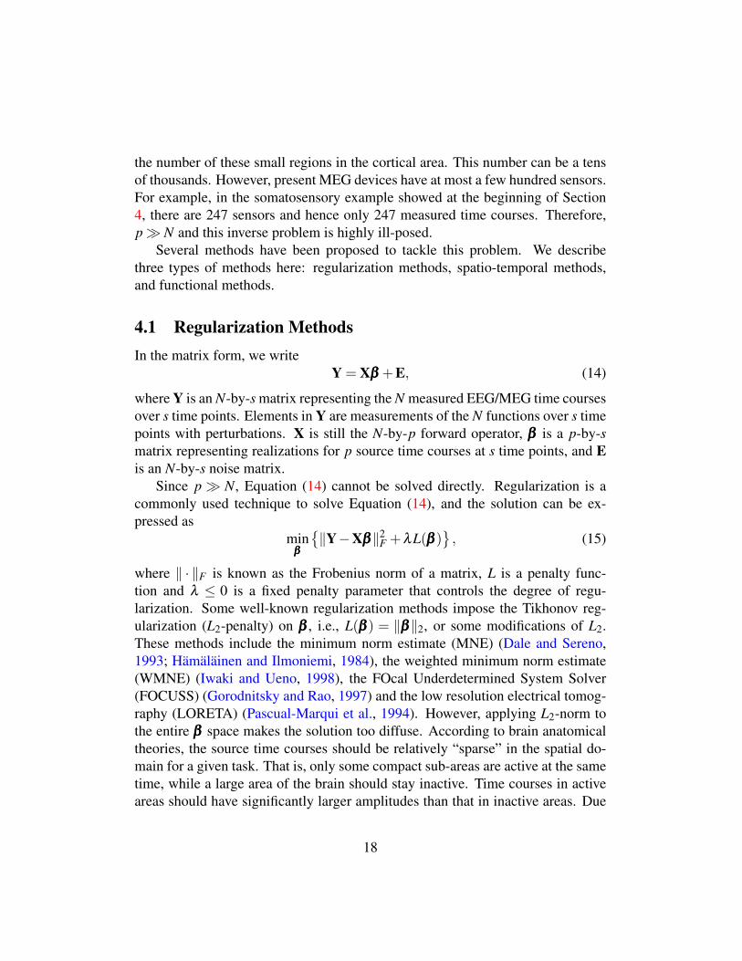
the number of these small regions in the cortical area. This number can be a tensof thousands. However, present MEG devices have at most a few hundred sensors.For example, in the somatosensory example showed at the beginning of Section4, there are 247 sensors and hence only 247 measured time courses. Therefore,p N and this inverse problem is highly ill-posed.

Several methods have been proposed to tackle this problem. We describethree types of methods here: regularization methods, spatio-temporal methods,and functional methods.

4.1 Regularization MethodsIn the matrix form, we write

Y = Xβββ +E, (14)

where Y is an N-by-s matrix representing the N measured EEG/MEG time coursesover s time points. Elements in Y are measurements of the N functions over s timepoints with perturbations. X is still the N-by-p forward operator, βββ is a p-by-smatrix representing realizations for p source time courses at s time points, and Eis an N-by-s noise matrix.

Since p N, Equation (14) cannot be solved directly. Regularization is acommonly used technique to solve Equation (14), and the solution can be ex-pressed as

minβββ

‖Y−Xβββ‖2

F +λL(βββ ), (15)

where ‖ · ‖F is known as the Frobenius norm of a matrix, L is a penalty func-tion and λ ≤ 0 is a fixed penalty parameter that controls the degree of regu-larization. Some well-known regularization methods impose the Tikhonov reg-ularization (L2-penalty) on βββ , i.e., L(βββ ) = ‖βββ‖2, or some modifications of L2.These methods include the minimum norm estimate (MNE) (Dale and Sereno,1993; Hamalainen and Ilmoniemi, 1984), the weighted minimum norm estimate(WMNE) (Iwaki and Ueno, 1998), the FOcal Underdetermined System Solver(FOCUSS) (Gorodnitsky and Rao, 1997) and the low resolution electrical tomog-raphy (LORETA) (Pascual-Marqui et al., 1994). However, applying L2-norm tothe entire βββ space makes the solution too diffuse. According to brain anatomicaltheories, the source time courses should be relatively “sparse” in the spatial do-main for a given task. That is, only some compact sub-areas are active at the sametime, while a large area of the brain should stay inactive. Time courses in activeareas should have significantly larger amplitudes than that in inactive areas. Due

18

to the nature of the L2-penalty, the results from L2-penalty based methods are toodiffuse in the spatial domain and are unsatisfactory in terms of localizing sparseactive areas.

One alternative to the L2-penalty is the minimum current estimate (MCE) andits modifications (Lin et al., 2006; Uutela et al., 1999), which impose the L1-penalty, i.e., L(βββ ) = |βββ |. MCE can produce better solutions in terms of iden-tifying sparse active areas due to the nature of the L1-penalty. However, MCEintroduces substantially discontinuities to the source time courses. Hence, the“spiky-looking” time courses will be observed. As described, the advantages anddisadvantages of L2 and L1 methods are complementary.

The aforementioned L2 and L1 based regularization methods were originallydesigned for parametric regression problems and are hardly applied to the non-parametric problems where β j(t)’s are smooth functions. Functional methods thattake into account the functional nature of the data are in strong demand. Thesemethods involving include the L1L2-norm inverse solver (Ou et al., 2009) and theFUNctional Expansion Regularization (FUNER) approach (Tian and Li, 2010).We briefly present these two methods in the following subsections.

4.2 A Spatio-Temporal MethodThe L1L2-norm method assumes the signal times courses the MEG time coursescan be represented by their lower-dimensional temporal basis functions. Thenit attempts to estimate their temporal coefficients instead of estimating the en-tire time courses. Since y(t) is evoked by βββ (t), it is natural to assume thatβββ (t) and y(t) share the same temporal bases. Suppose that y(t) and βββ (t) canbe approximated by the same K-dimensional temporal basis. That is, we letyi(t) = ∑

Kk=1 ψk(t)yi,k and β j(t) = ∑

Kk=1 ψk(t)β j,k, where ψk(t) is the kth basis

function, yi,k is the kth coefficient for the ith MEG time course and β j,k is the kthcoefficient for the jth source time course. Then Model (14) can be simplified by

Y = Xβββ + E, (16)

where Y, βββ and E are all N-by-K coefficient matrices for their basis functions. Asmooth temporal domain and a sparse spatial domain can be achieved by imposingan L2-penalty to the temporal domain and an L1-penalty to the spatial domain, i.e.,

L(βββ ) =N

∑n=1

√√√√ K

∑k=1

β 2N,k. (17)

19

Then the minimization problem can be treated as a second-order cone program-ming problem and hence solved.

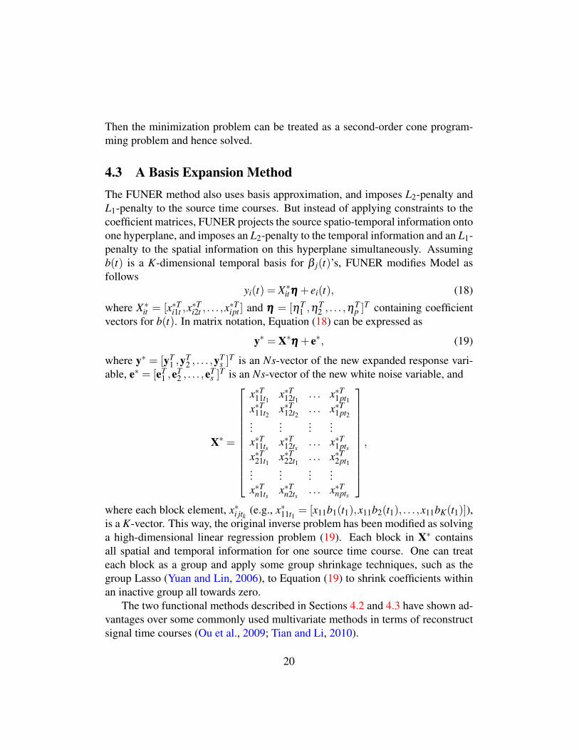
4.3 A Basis Expansion MethodThe FUNER method also uses basis approximation, and imposes L2-penalty andL1-penalty to the source time courses. But instead of applying constraints to thecoefficient matrices, FUNER projects the source spatio-temporal information ontoone hyperplane, and imposes an L2-penalty to the temporal information and an L1-penalty to the spatial information on this hyperplane simultaneously. Assumingb(t) is a K-dimensional temporal basis for β j(t)’s, FUNER modifies Model asfollows

yi(t) = X∗itηηη + ei(t), (18)

where X∗it = [x∗Ti1t ,x∗Ti2t , . . . ,x

∗Tipt ] and ηηη = [ηT

1 ,ηT2 , . . . ,η

Tp ]

T containing coefficientvectors for b(t). In matrix notation, Equation (18) can be expressed as

y∗ = X∗ηηη + e∗, (19)

where y∗ = [yT1 ,y

T2 , . . . ,y

Ts ]

T is an Ns-vector of the new expanded response vari-able, e∗ = [eT

1 ,eT2 , . . . ,e

Ts ]

T is an Ns-vector of the new white noise variable, and

X∗ =

x∗T11t1 x∗T12t1 . . . x∗T1pt1x∗T11t2 x∗T12t2 . . . x∗T1pt2...

......

...x∗T11ts x∗T12ts . . . x∗T1ptsx∗T21t1 x∗T22t1 . . . x∗T2pt1...

......

...x∗Tn1ts x∗Tn2ts . . . x∗Tnpts

,

where each block element, x∗i jtk (e.g., x∗11t1 = [x11b1(t1),x11b2(t1), . . . ,x11bK(t1)]),is a K-vector. This way, the original inverse problem has been modified as solvinga high-dimensional linear regression problem (19). Each block in X∗ containsall spatial and temporal information for one source time course. One can treateach block as a group and apply some group shrinkage techniques, such as thegroup Lasso (Yuan and Lin, 2006), to Equation (19) to shrink coefficients withinan inactive group all towards zero.

The two functional methods described in Sections 4.2 and 4.3 have shown ad-vantages over some commonly used multivariate methods in terms of reconstructsignal time courses (Ou et al., 2009; Tian and Li, 2010).

20

4.4 An ExampleIn this section, we provide comparisons of the FUNER method and two regular-ization methods: MNE and MCE on an real-world MEG data. The data were fromthe somatosensory study described in the beginning of Section 4. The data wereobtained from the Center for Clinical Neurosciences at the University of TexasHealth Science Center. For the FUNER method, we apply two bases: NCS withK = 7 bases functions and the first K = 7 bases from singular value decomposition(SVD) of Y.

We are interested in the activation map at time points 85 and 99. Figure 3shows side views of the 3-D brain maps at time point 85 by the three methods.Among these four figures, FUNER with SVD bases is the best because it cor-rectly identifies the somatosensory area (located at the left postcentral gyrus) andthe active area is very focal. MCE is the second best because it also correctlyidentifies part of the somatosensory area but the active area is not large enough.The active area from FUNER with a NCS basis is too focal, so this method isrelatively less satisfactory comparing to FUNER (SVD) and MCE. MNE is theworse method among the four methods, because the active areas from MNE aretoo broad. It picks out the somatosensory area but also incorrectly picks out someinactive areas.

We also examine the computation cost in this example. All methods are imple-mented in R and the computation time is recorded in Table 4. As we can see, theexecution time for FUNER is much higher than MNE and MCE. This is becauseFUNER expands the data to a higher-dimensional space and makes the alreadylarge data even larger.

This example shows that some functional methods can provide better resultsthan multivariate methods in terms of accuracy, but the computation cost may behigh.

Table 4: Execution time in second.

MNE MCE FUNER (NCS)CPU Time 874 1137 6127

21

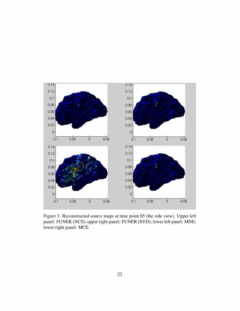
Figure 3: Reconstructed source maps at time point 85 (the side view). Upper leftpanel: FUNER (NCS); upper right panel: FUNER (SVD); lower left panel: MNE;lower right panel: MCE.

22

5 Conclusions and DiscussionsFDA applied on functional brain imaging studies has become more and moreprevalent nowadays. We have briefly discussed three issues, dimension reduc-tion, spatial classification and the inverse problem, that occur in functional brainimaging studies. They are problems with strong demands on FDA techniques.

There are three major challenges in applying FDA to functional brain imag-ing studies. First and foremost, the computational cost is a big issue due to thelarge volume of brain imaging data. In particular, when some method requires astochastic search or an expansion of the data by their basis functions, the issue willbe aggravated (see Tables 2 and 4). Although most of the brain imaging problemsfocus on accuracy rather than real-time processing performance, computation ef-ficiency is still an important factor to consider. Second, most FDA techniques thatdeal with brain imaging data assume that the error term is independent and iden-tically distributed white noise. However, the noise is rarely normally distributed.For example, in fMRI studies, sources of noise include low-frequency drift dueto machine imperfections, oscillatory noise due to respiration and cardiac pulsa-tion, residual movement artefacts and so on. Further investigation that considersdifferent noise patterns and dependencies is needed. Third, since brain imagesare naturally 3-dimensional, the observed times courses are not independent fromeach other. Correlations are higher between time courses in a neighboring regionthan that between time courses that are far away. Therefore, spatial propertiesshould be taken into considerations as well.

There are many other issues and problems also desire FDA, such as the EEG/MEGsensor evaluation and fMRI pattern classification. The former needs to identifyimportant sensors based on the measured time courses from multiple subjects(Coskun et al., 2009). One of the most commonly used techniques is the T-test,which is far from satisfactory. More sophisticated FDA techniques should be in-vestigated and applied. The latter needs to identify brain state associated with astimulus. A large amount of research devoted to machine learning methods [see,for example, (Martinez-Ramon et al., 2006; Pereira et al., 2009; Tian et al., 2010)].However, less research has been conducted on FDA techniques even though theyare just as useful as machine learning techniques. FDA methods should also beinvestigated for these problems.

23

ReferencesAggarwal, C. C., A. Hinneburg, and D. A. Keim (2001). On the surprising behav-

ior of distance metrics in high dimensional space. In Lecture Notes in ComputerScience, London, UK, pp. 420–434. Springer-Verlag.

Alter, O., P. Brown, and D. Bostein (2000). Singular value decomposition forgenome-wide expression data processing and modeling. Proceedings of theNational Academy of Sciences of the United States 97, 10101–10106.

Barlow, H. B. (1994). What is the computational goal of the neocortex? InC. Koch and J. L. Davis (Eds.), Large-scale neuronal theories of the brain, pp.1–22. Cambridge, MA: MIT press.

Bellman, R. (1957). Dynamic Programming. Princeton, NJ: Princeton UniversityPress.

Breiman, L. (2001). Random forests. Machine Learning 45, 5–32.

Candes, E. and T. Tao (2007). The dantzig selector: Statistical estimation when pis much larger than n (with discussion). Annals of Statistics 35(6), 2313–2351.

Coskun, M. A., L. Varghese, S. Reddoch, E. M. Castillo, D. A. Pearson, K. A.Loveland, A. C. Papanicolaou, and B. R. Sheth (2009). Increased responsevariability in autistic brains? NeuroReport 20(17), 1543–1548.

Cuevas, A., M. Febrero, and R. Fraiman (2007). Robust estimation and classifi-cation for functional data via projection-based depth notions. ComputationalStatistics 22, 481–496.

Dale, A. M. and M. I. Sereno (1993). Improved localization of cortical activityby combining eeg and meg with mri cortical surface reconstruction: A linearapproach. Journal of Cognitive Neuroscience 5, 162–176.

Di, C.-Z., C. M. Crainiceanu, B. S. Caffo, and N. M. Punjabi (2009). Multilevelfunctional principal component analysis. Annals of Applied Statistics 3(1), 458–488.

Efron, B., T. Hastie, I. Johnstone, and R. Tibshirani (2004). Least angle regres-sion. Annals of Statistics 32, 407–451.

24

Ermer, J. J., J. C. Mosher, S. Baillet, and R. M. Leahy (2001). Rapidly recom-putable eeg forward models for realistic head shapes. Physics in Medicine andBiology 46, 1265–1281.

Fan, J. and R. Li (2001). Variable selection via nonconcave penalized likelihoodand its oracle properties. Journal of the American Statistical Association 96,1348–1360.

Ferraty, F. and P. Vieu (2003). Curves discrimination: a nonparametric functionalapproach. Computational Statistics & Data Analysis 44, 161–173.

Ferraty, F., P. Vieu, and S. Viguier-Pla (2007). Factor based comparison of groupsof curves. Computational Statistics & Data Analysis 51, 4903–4910.

Gorodnitsky, I. F. and B. D. Rao (1997). Sparse signal reconstruction from limiteddata using focuss: a re-weighted minimum norm algorithm. Signal Processing,IEEE Transactions on 45(3), 600–616.

Hall, P., D. S. Poskitt, and B. Presnell (2001). A functional data-analytic approachto signal discrimination. Technometrics 43(1), 1–9.

Hamalainen, M. and R. J. Ilmoniemi (1984). Interpreting measured magneticfields of the brain: estimates of current distribution. Technical report, HelsinkiUniversity of Technology. TKK-F-A599.

HERTZ, J., A. KROGH, and R. G. PALMER (1991). Introduction to the Theoryof Neural Computation. Reading, MA: Addison-Wesley.

Ho, M.-h. R., H. Ombao, J. C. Edgar, J. M. Canive, and G. A. Miller (2008).Time-frequency discriminant analysis of meg signals. NeuroImage 40(1), 174–186.

Iwaki, S. and S. Ueno (1998). Weighted minimum-norm source estimation ofmagnetoencephalography utilizing the temporal information of the measureddata. Journal of Applied Physics 83(11), 6441–6443.

James, G. (2002). Generalized linear models with functional predictors. Journalof the Royal Statistical Society: Series B 64, 411–432.

James, G. and T. Hastie (2001). Functional linear discriminant analysis for irreg-ularly sampled curves. Journal of the Royal Statistical Society: Series B 63,533–550.

25

Lin, F.-H., J. W. Belliveau, A. M. Dale, and M. S. Hamalainen (2006). Dis-tributed current estimates using cortical orientation constraints. Human BrainMapping 27, 1–13.

Long, C., E. Brown, C. Triantafyllou, I. Aharon, L. Wald, and V. Solo (2005).Nonstationary noise estimation in functional mri. Neuroimage 28, 890–903.

Martinez-Ramon, M., V. Koltchinskii, G. Heilman, and S. Posse (2006). fmripattern classification using nueroanatomically constrained boosting. Neuroim-age 31, 1129–1141.

Mosher, J., P. Lewis, and R. Leahy (1992). Multiple dipole modeling and lo-calization from spatio-temporal meg data. IEEE Transactions on BiomedicalEngineering 39(6), 541–557.

Mosher, J. C., R. M. Leahy, and P. S. Lewis (1999). Eeg and meg: forwardsolutions for inverse methods. IEEE Transactions on Biomedical Engineer-ing 46(3), 245–259.

Muller, H. G. (2005). Functional modelling and classification of longitudinal data.Scandinavian Journal of Statistics 32, 223–240.

Muller, H. G. and U. Stadtmuller (2005). Generalized functional linear models.Annals of Statistics 33(2), 774–805.

Nason, G. P., R. von Sachs, and G. Kroisandt (1999). Wavelet processes andadaptive estimation of the evolutionary wavelet spectrum. Journal of the RoyalStatistical Society: Series B 62, 271–292.

Ombao, H., R. von Sachs, and W. Guo (2005). Slex analysis of multivariatenonstationary time series. Journal of the American Statistical Association 100,519–531.

Ou, W., M. Hamalainen, and P. Golland (2009). A distributed spatio-temporaleeg/meg inverse solver. Neuroimage 44(3), 932–46.

Pascual-Marqui, R. D., M. C. M, and L. D (1994). Low resolution electromag-netic tomography: a new method for localizing electrical activity in the brain.International Journal of Psychophysiology 18, 49–65.

Pereira, F., T. Mitchell, and M. Botvinick (2009). Machine learning classifiersand fmri: a tutorial overview. Neuroimage 45, 199–209.

26

Radchenko, P. and G. James (2008). Variable inclusion and shrinkage algorithms.Journal of the American Statistical Association 103, 1304–1315.

Radchenko, P. and G. James (2010). Forward-lasso with adaptive shrinkage. An-nals of Statistics. in press.

Ramsay, J. and B. Silverman (2005). Functional Data Analysis (Second Edition).New York, NY: Springer.

Ramsay, J. O. and C. Dalzell (1991). Some tools for functional data analysis (withdiscussion). Journal of the Royal Statistical Society: Series B 53, 539–572.

Roberts, T. P. and D. Poeppel (1996). Latency of auditory evoked m100 as afunction of tone frequency. Neuroreport 7(6), 1138–1140.

Tian, T. S. and G. M. James (2010). Interpretable dimensionality reduction forclassification with functional data. Under review.

Tian, T. S., G. M. James, and R. R. Wilcox (2010). A multivariate stochasticsearch method for dimensionality reduction in classification. Annals of AppliedStatistics 4(1), 339–364.

Tian, T. S. and Z. Li (2010). Funer: A novel approach for the eeg/meg inverseproblem. Under review.

Tibshirani, R. (1996). Regression shrinkage and selection via the lasso. Journalof the Royal Statistical Society: Series B 58, 267–288.

Tibshirani, R. and T. Hastie (2007). Margin trees for high-dimensional classifica-tion. Journal of Machine Learning Research 8, 637–652.

Tibshirani, R., T. Hastie, B. Narasimhan, and G. Chu (2002). Diagnosis of multi-ple cancer types by shrunken centroids of gene expression. Proceedings of theNational Academy of Sciences of the United States 99(10), 6567–6572.

Uutela, K., M. Hamalainen, and E. Somersalo (1999). Visualization of magne-toencephalographic data using minimum current estimates. NeuroImage 10,173–180.

VanVeen, B., W. van Drongelen, M. Yuchtman, and A. Suzuki (1997). Local-ization of brain electrical activity via linearly constrained minimum variancespatial filtering. IEEE Transactions on Biomedical Engineering 44, 867C880.

27

Vapnik, V. (1998). Statistical Learning Theory. New York: Wiley.

Viviani, R., G. Gron, and M. Spitzer (2005). Functional principal componentanalysis of fmri data. Human Brain Mapping 24, 109–129.

Wu, Y.-l., D. Agrawal, and A. E. Abbadi (2000). A comparison of dft and dwtbased similarity search in time-series databases. In In Proceedings of the 9 th In-ternational Conference on Information and Knowledge Management, McLean,VA, pp. 488–495.

Yuan, M. and Y. Lin (2006). Model selection and estimation in regression withgrouped variables. Journal of the Royal Statistical Society: Series B 68, 49–67.

Zhang, Y., B. Pham, and M. Eckstein (2006). The effect of nonlinear humanvisual system components on performance of a channelized hotelling observerin structured backgrounds. IEEE Transactions on Medical Imaging 25(10),1348–1362.

Zou, H. and T. Hastie (2005). Regularization and variable selection via the elasticnet. Journal of the Royal Statistical Society: Series B 67, 301–320.

28