Embed Size (px)
Citation preview

http://fun3d.larc.nasa.gov
FUN3D v13.4 Training
Session 8:
Supersonic and Hypersonic
Perfect Gas Simulation
Mike Park
1FUN3D Training Workshop
December 11-12, 2018

http://fun3d.larc.nasa.gov
Session Overview• How to use FUN3D to compute perfect gas supersonic and
hypersonic flows (eqn_type=“compressible”)
• What are the challenges and strategies
• Inviscid flux types and inviscid flux gradient limiters options that work the best for supersonic and hypersonic flows
• Required practice for running adjoint with gradient limiters for design and grid adaptation
• Methods to initialize supersonic and hypersonic flows
• Example of a hypersonic flow application
• What to do when things go wrong
• The focus is on high-speed flows, but the strategies discussed can be used in other flow regimes
22FUN3D Training Workshop
December 11-12, 2018

http://fun3d.larc.nasa.gov
Perfect and Generic Gas Simulation• The input parameters described in this talk are only valid for
(eqn_type=“compressible”)
• Generic gas input parameters are different, but the philosophy is similar
• Work is underway to merge the options where possible, but consult generic gas specific documentation for details
3FUN3D Training Workshop
December 11-12, 20183

http://fun3d.larc.nasa.gov 4
• The inviscid terms can be discontinuous, i.e., when there are shocks
– Entropy problem: strong shocks can cause difficulties in inviscid flux
schemes especially near points in the flow where the dissipation
vanishes
– Monotonicity problem: shocks cause discontinuities that make robust
implementation of higher order schemes difficult
• The inviscid terms can be a problem when there is strong expansion
– Positivity problem: strong expansions can cause difficulties such that
the local conditions approach a vacuum
– Sonic rarifaction or “expansion shock” problem: strong expansions near
the sonic point where dissipation due to the u-a eigenvalues vanishes
can cause difficulties
• Turbulence modeling challenges compound these issues but are not
the focus of this talk
What Are the Challenges?
FUN3D Training Workshop December 11-12, 2018
4

http://fun3d.larc.nasa.gov
• Inviscid flux schemes fall into several categories:
• Contact preserving, i.e., good for viscous flows
• Flux difference splitting scheme of flux_construction = “roe”
• Non positivity near vacuum conditions
• The sonic rarefaction problem
• The “carbuncle” problem
• Non preservation of the total enthalpy in shocks
• Entropy fixes (Eigenvalue smoothing) exist for some but not all of these
problems
• Flux splitting schemes such as flux_construction = “hllc” and
“ldfss” may display some limited unphysical behavior at very strong
normal shocks
• Non-contact preserving, i.e., not usually good for viscous flows
• Flux vector split scheme, flux_construction =”vanleer”, has
desirable qualities
• Positivity near vacuum conditions
• Preservation of the total enthalpy in shocks
Inviscid Flux Types
5FUN3D Training Workshop
December 11-12, 20185

http://fun3d.larc.nasa.gov
• Inviscid flux schemes fall into several categories:
• Hybrid or “blended” schemes
• The flux_construction = “dldfss” scheme is a blend of two schemes
• The vanleer scheme at shocks via a shock detector
• The ldfss scheme near walls via a shock and boundary layer detector
Inviscid Flux Types
6FUN3D Training Workshop
December 11-12, 20186

http://fun3d.larc.nasa.gov
Inviscid Flux Gradient Limiter Types• Gradient limiters are available in two types:
• Edge based : limiting is done on an edge by edge basis, flux_limiter = “minmod”, “vanleer”, “vanalbada” and “smooth”
• They are less dissipative and they work pretty well on hex grids but
they are not as robust on mixed element or tetrahedral grids.
• They are not “freezable” and may cause convergence to get hung up
by limiter cycling. They also cannot be used when using the adjoint
solvers
• Stencil based : limiting is done based on the max and min reconstructed
higher order edge gradients that exist over the entire control volume “stencil”, flux_limiter = “barth”, “hvanleer”, “hvanalbada”, “hsmooth”, and “venkat”
• They are more robust but more dissipative and work on all grid types
• They are “freezable”, i.e., can be frozen after a suitable number of
iterations, which sometimes will allow the solution to converge further
• They must be frozen when solving adjoint equations
• Limiters with the “h” prefix include a heuristic stencil based pressure
limiter to increase robustness
7FUN3D Training Workshop
December 11-12, 20187

http://fun3d.larc.nasa.gov
Inviscid Flux Gradient Limiter Tips• Gradient limiter selection is problem specific, make sure you experiment with
your case
• Some limiters are dimensional, see smooth_limiter_coef documentation
in the manual
• This can increase or decrease the limiter effect
• Recent experience with finer grids have changed some preferences formed on
the coarse grids used a decade ago
8FUN3D Training Workshop
December 11-12, 20188

http://fun3d.larc.nasa.gov
Realizability
• Nonphysical (negative density or pressure) reconstructions are set
to cell averages (first order) accompanied with a “realizability”
warning
• Nonlinear density and pressure updates are floored to a ratio of freestream with the f_allow_minimum_m namelist variable
• The default floor may need to be lowered if the simulation
requires it
9FUN3D Training Workshop
December 11-12, 20189

http://fun3d.larc.nasa.gov
Calorically Perfect Supersonic Flow
• Maximum Mach number in computational domain < 3.0 such that:
• Shocks are relatively weak
• Expansion fans are relatively weak
• Inviscid flux options suitable for these applications:
• When Euler: viscous_terms = “inviscid”
• flux_construction = “vanleer”, “ldfss”, “hllc” or “roe”
• When Navier-Stokes: viscous_terms = “laminar” or “turbulent”
• flux_construction = “ldfss”, “hllc”, or “roe”
• Inviscid flux gradient limiter options most suitable for these applications:
• flux_limiter = “vanleer”, “vanalbada”, “hvanleer”, or
“hvanalbada”
• For applications that require solving the adjoint:
• flux_construction = “vanleer” or “roe”
• flux_limiter = “hvanleer” or “hvanalbada”
10FUN3D Training Workshop
December 11-12, 201810

http://fun3d.larc.nasa.gov
Calorically Perfect Hypersonic Flow
• Maximum Mach number in computational domain > 3.0 such that:
• Shocks may be strong, especially when there are normal shocks
• Expansion fans may be strong
• Inviscid flux options suitable for these applications:
• When Euler: viscous_terms = “inviscid”
• flux_construction = “vanleer” or “dldfss”
• When Navier-Stokes: viscous_terms = “laminar” or
“turbulent”
• flux_construction = “dldfss”
• Inviscid flux gradient limiter options most suitable for these
applications:
• flux_limiter = “hvanleer” or “hvanalbada”
• For applications that require solving the adjoint:
• flux_construction = “vanleer” or “roe”
• flux_limiter = “hvanleer” or “hvanalbada”
11FUN3D Training Workshop
December 11-12, 201811

http://fun3d.larc.nasa.gov
Nonlinear Equations
• When solving nonlinear equations (e.g., Euler, Navier-Stokes), the
initial guess is critical!
• Transients can be much more challenging than the steady solution
• Solution under and over shoots can be aggravated
• Nonphysical states may be transited
• Boundary conditions are less robust with large gradients nearby
• Linear system solution scheme and nonlinear defect correction
solution schemes can become unstable
12FUN3D Training Workshop
December 11-12, 201812

http://fun3d.larc.nasa.gov
Strategy
• Perform the simulation in phases
• Initialization
• Target solution scheme
• Optional end game that freezes limiter for better iterative
convergence.
• Initialization is the primary challenge to success for high speed,
internal, and propulsion flows
13FUN3D Training Workshop
December 11-12, 201813

http://fun3d.larc.nasa.gov
Initialization Strategies
• The default initialization fills the domain with freestream flow and
applies strong boundary conditions
• Creates high gradients adjacent to the boundary
• Sets up an unphysical expansion on backward facing surfaces
• The goal of initialization is to improve this default flow field with one
that establishes the physical mechanisms of the simulations (e.g.,
boundary layers, shear layers, recirculation zones)
• Moves large gradient regions away from the boundaries and into
the interior of the domain
• You have the freedom to use methods that are inaccurate as long as
you later restart the solution with an appropriate method for your
simulation
• Includes changing boundary conditions, freestream conditions,
etc.
14FUN3D Training Workshop
December 11-12, 201814

http://fun3d.larc.nasa.gov
Initialization Strategies
• Use first_order_iterations to create a spatially first-order
solution
• This helps the nonlinear update because there are less
approximations in defect correction
• Use a more dissipative flux scheme
• Roe with excessive Eigenvalue smoothing
• rhs_u_eigenvalue_coef, lhs_u_eigenvalue_coef,
rhs_a_eigenvalue_coef, lhs_a_eigenvalue_coef
• “vanleer” for Navier-Stokes
• Restart from a lower Mach number or angle of attack solution
• Slow down (lower CFL number or physical time step)
• This aids the stability of the linear solve and nonlinear updates
• Combinations of these strategies
15FUN3D Training Workshop
December 11-12, 201815

http://fun3d.larc.nasa.gov
Initialization Strategies
• Explicitly initialize with the &flow_initialization namelist
• Fill plenums with subsonic high density and pressure gas
• Place a subsonic wake behind an aft facing step
• Surround the entire vehicle with a sphere of post shock flow
conditions (subsonic high density and pressure gas)
• May reduce the execution time by allowing the use of larger CFL
numbers
16FUN3D Training Workshop
December 11-12, 201816

http://fun3d.larc.nasa.gov
Solution Scheme
• See the advantages and disadvantages of the available fluxes and
limiters
• Adjust (ramp) the CFL number for the best convergence rate
• Expect the solution convergence to stall due to limiter buzz
17FUN3D Training Workshop
December 11-12, 201817

http://fun3d.larc.nasa.gov
End Game
• Optionally freeze the gradient limiter to overcome limiter buzz
• Make sure the solution is sufficiently converged
18FUN3D Training Workshop
December 11-12, 201818

http://fun3d.larc.nasa.gov
Multiple Step Approach
• Applications with shocks and expansions may need to be run in
multiple steps
• Step 1 : Run solution first order while scheduling the CFL number to
evolve the solution to a quasi-steady state;
• Initialize the flow appropriately
• Set first_order_iterations to the same as the number of iterations
specified by steps
• Use schedule_iteration, schedule_cfl, and schedule_cflturb to
slowly increase CFL number
• Step 2 : Restart solution higher order while scheduling the CFL number
to compute the final solution;
• Read the restart file, i.e. restart_read = “on”
• Set first_order_iterations = 0
• The CFL ramping of schedule_iteration, schedule_cfl, and
schedule_cflturb may need to be less aggressive
19FUN3D Training Workshop
December 11-12, 201819
http://fun3d.larc.nasa.gov
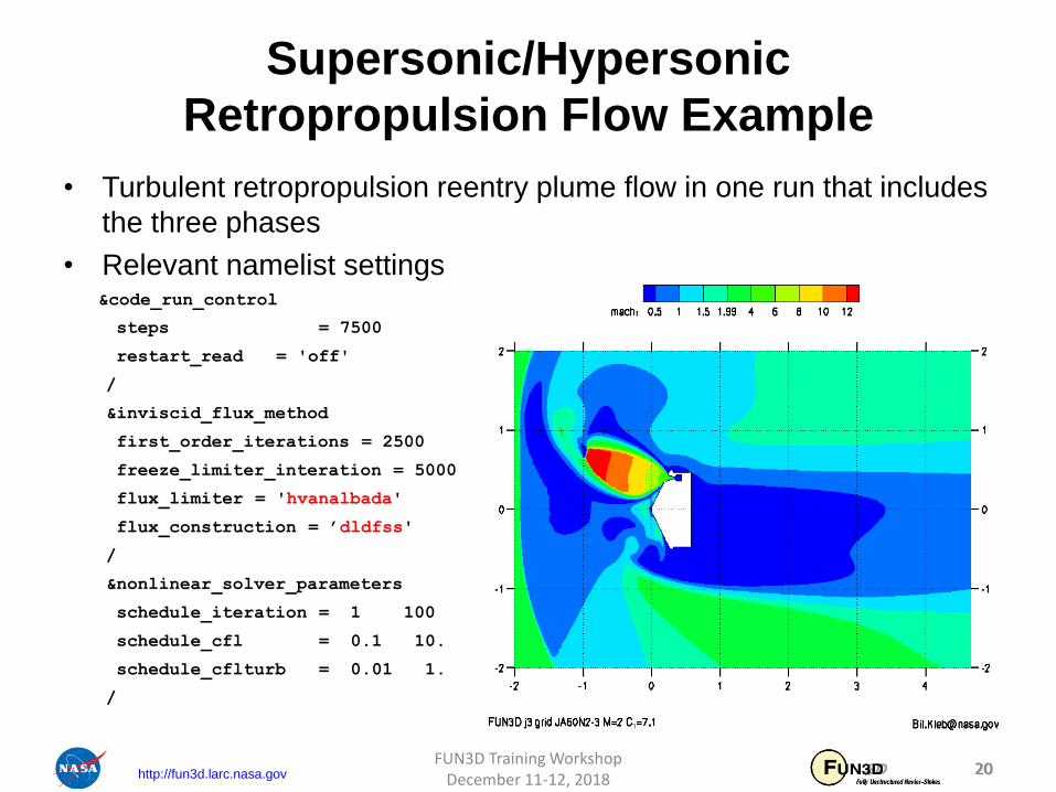
Supersonic/Hypersonic
Retropropulsion Flow Example
• Turbulent retropropulsion reentry plume flow in one run that includes
the three phases
• Relevant namelist settings&code_run_control
steps = 7500
restart_read = 'off'
/
&inviscid_flux_method
first_order_iterations = 2500
freeze_limiter_interation = 5000
flux_limiter = 'hvanalbada'
flux_construction = ’dldfss'
/
&nonlinear_solver_parameters
schedule_iteration = 1 100
schedule_cfl = 0.1 10.
schedule_cflturb = 0.01 1.
/
20FUN3D Training Workshop
December 11-12, 201820

http://fun3d.larc.nasa.gov
Supersonic/Hypersonic
Retropropulsion Flow Example• Switch from 1st-order to 2nd-order scheme occurs at 2500 iterations
• The hvanalbada limiter was frozen at 5000 iterations
• Continuity and energy equation residuals converged ~4 orders
• Jet unsteadiness probably preventing further convergence
• Lift has converged, i.e., is no longer changing
21FUN3D Training Workshop
December 11-12, 201821

http://fun3d.larc.nasa.gov
Supersonic/Hypersonic
Retropropulsion Flow Example
Some Observations• Turbulent flow has made this case easier to run because of the
added dissipation caused by the eddy viscosity in the retro-
propulsion jet
• If this case were laminar, it would probably be more difficult to run
- You would need to be careful that the dldfss flux scheme does
not add too much dissipation by refining the grid
- You may need to resort to a multiple step running approach or
explicit initialization of the flow field
2222FUN3D Training Workshop
December 11-12, 2018

http://fun3d.larc.nasa.gov 23
Diagnosis When Things Go Wrong
• Restart the solution and visualize just before an increase in the
residual
• Create movies near the largest residual location
• Try to isolate the problem location
• Check your grid resolution near the maximum residual location
– Under-resolved expansions can cause a lot of trouble
– Really large grid aspect ratios near expansions can cause trouble
• Check to make sure your boundary conditions are well posed
• This is especially true for internal flows
23FUN3D Training Workshop
December 11-12, 2018

http://fun3d.larc.nasa.gov 24
Diagnosis When Things Go Wrong
• Isolate the problem to linear system or nonlinear update
• Set linear_projection = .true. or change the number of
linear sweeps
• Lowering CFL number can aid linear and nonlinear stability
• Try a different initialization strategy
24FUN3D Training Workshop
December 11-12, 2018

http://fun3d.larc.nasa.gov 25
• Recommended use cases and descriptions of flux schemes
• Recommended use cases for gradient limiters and how to freeze
them
• Initialization strategies
• What the convergence behavior may look like
• What to do when things go wrong
What We Learned
25FUN3D Training Workshop
December 11-12, 2018