Fully Automatic Segmentation of the Proximal Femur …Fully Automatic Segmentation of the Proximal ... CLM-based contour extraction yields a robust and fully auto- ... dependent on

IEEE TRANSACTIONS ON MEDICAL IMAGING 1

Fully Automatic Segmentation of the ProximalFemur Using Random Forest Regression VotingC. Lindner*, S. Thiagarajah, J.M. Wilkinson, The arcOGEN Consortium, G.A. Wallis and T.F. Cootes

Abstract—Extraction of bone contours from radiographs playsan important role in disease diagnosis, pre-operative planning,and treatment analysis. We present a fully automatic method toaccurately segment the proximal femur in anteroposterior pelvicradiographs. A number of candidate positions are produced bya global search with a detector. Each is then refined using astatistical shape model together with local detectors for eachmodel point. Both global and local models use Random Forestregression to vote for the optimal positions, leading to robustand accurate results. The performance of the system is evaluatedusing a set of 839 images of mixed quality. We show that the localsearch significantly outperforms a range of alternative matchingtechniques, and that the fully automated system is able to achievea mean point-to-curve error of less than 0.9mm for 99% ofall 839 images. To the best of our knowledge, this is the mostaccurate automatic method for segmenting the proximal femurin radiographs yet reported.

Index Terms—automatic femur segmentation, femur detection,Random Forests, Hough Transform, Constrained Local Models.

I. I NTRODUCTION

I N clinical practice, plain film radiographs are widely usedto assist in disease diagnosis, pre-operative planning and

treatment analysis. Extraction of the contours of the proximalfemur from anteroposterior (AP) pelvic radiographs plays animportant role in diseases such as osteoarthritis (e. g. diagnos-tics and joint-replacement planning) or osteoporosis (e. g. frac-ture detection and bone density measurements). In addition,accurately segmenting the contours of the proximal femur inradiographs allows monitoring of disease progression.

Manual segmentation of the proximal femur in radiographsis time-consuming and hard to do consistently. Our aim is toautomate the segmentation procedure. Fully automatic proxi-mal femur segmentation is challenging for several reasons:(i)The quality of radiographs may vary considerably in terms ofcontrast, resolution and the region of the pelvis shown.(ii)AP pelvic radiographs only give a 2D projection of what is a3D object, and hence are susceptible to rotational issues; thesame 3D shape may yield a different 2D projection depending

Copyright (c) 2013 IEEE. Personal use of this material is permitted.However, permission to use this material for any other purposes must beobtained from the IEEE by sending a request to [email protected].

The arcOGEN Consortium is funded by Arthritis Research UK and C. Lind-ner by the Medical Research Council.Asterisk indicates corresponding author.

C. Lindner is with the Centre for Imaging Sciences, The University ofManchester, U.K. (e-mail: [email protected]).

S. Thiagarajah and J.M. Wilkinson are with the Department of HumanMetabolism, The University of Sheffield, U.K.

G.A. Wallis is with the Wellcome Trust Centre for Cell Matrix Research,The University of Manchester, U.K.

T.F. Cootes is with the Centre for Imaging Sciences, The University ofManchester, U.K.

on the view point.(iii) Plain film radiographs do not providehomogeneous values for the same structure due to overlappingbody parts.(iv) Deformities of the proximal femur may causethe loss of distinguishable radiographic key features.

Automatically extracting the contours of the proximal femurcomprises two key steps: Firstly, the femur is detected in theimage and secondly, the contours are segmented. We proposeto use Random Forest regression voting in a sliding windowapproach to fully automatically segment the proximal femur.

Random Forests (RF) [1] describe an ensemble of decisiontrees trained independently on a randomised selection offeatures. They have been shown to be effective in a widerange of classification and regression problems [2], [3], [4].Recent work on Hough Forests [5] has shown that objectscan be effectively located by training RF regressors to predictthe position of a point relative to the sampled region, thenrunning the regressors over a region and accumulating votesfor the likely position. To detect the proximal femur, our globalsearch uses a RF regressor that votes for the centre of areference frame, resulting in a Hough-like [6] response imageof accumulated votes. The approximated position is then usedto initialise a local search to segment the femur, combininglocal detectors with a statistical shape model. Following [7],we apply RF regression in the Constrained Local Model(CLM) framework to vote for the optimal position of eachmodel point. In the CLM framework, feature detectors are runindependently to generate response images for each point andthen a shape model is used to find the best combination ofpoints [8].

Using RF regression voting for both object detection andCLM-based contour extraction yields a robust and fully auto-matic segmentation system. We use the latter to segment theproximal femur in AP pelvic radiographs. Preliminary outputsof this work were presented in [9]. This paper expands onthe latter in that it describes several improvements to thealgorithm yielding significantly higher segmentation accuracy.We show additional in-depth experimental results, and allmethods are evaluated on a larger data set of 839 images.We demonstrate that results are very accurate and that boththe local search and the fully automatic search outperformalternative matching techniques such as Active Shape Models(ASMs) [10], Active Appearance Models (AAMs) [11], andCLMs using normalised correlation and intensity probability-based search. We believe this to be the most accurate fullyautomatic femur segmentation system yet published.

This is the author’s version of an article that has been published in this journal. Changes were made to this version by the publisher prior to publication.The final version of record is available athttp://dx.doi.org/10.1109/TMI.2013.2258030

Copyright (c) 2013 IEEE. Personal use is permitted. For any other purposes, permission must be obtained from the IEEE by emailing [email protected].


II. RELATED WORK

There are different approaches for automatising the segmen-tation of contours from medical images such as threshold-based methods, atlas-based techniques or deformable models.Our approach falls into the category of deformable models.Behiels et al. [12] have shown that statistical shape modelscan be successfully used to segment the proximal femur, giventhat a good initialisation for the model is available. Zhenget al. [13] have introduced Marginal Space Learning as aneffective approach for object detection. This aims to initialisea shape model by estimating pose, orientation and scale insequence rather than exhaustively searching the full parameterspace. This speeds up the searching procedure but might notfind the optimal solution.

The idea of using a Hough like approach in combinationwith a deformable model to automatically segment the proxi-mal femur is not new. Pilgram et al. [14] as well as Smith etal. [15] have suggested to use Hough straight line detection.The latter as well as the atlas-based approach by Ding etal. [16] rely on the results of a Canny edge detector [17]for identifying the femoral shafts. However, most publishedmethods make assumptions about the femur pose and weretested on data sets with very similar image quality across theset. Our technique is shown to deal with a wide range of imagequality and femur pose.

III. M ETHODS

In the following, we introduce Random Forest regressionvoting and Constrained Local Models both of which are atthe core of the fully automated segmentation system to bepresented in Section IV.

A. Voting with Random Forest regression

We use RF regression in a similar manner to the HoughForests approach [5]. However, in our case due to the consis-tent skeletal anatomy across individuals from one radiographto the other, almost any part of the image can predict the areawe are interested in. Hence, we do not require voting to bedependent on a class label, allowing all image structures tovote. In addition, Hough Forests use RFs whose leaves storemultiple training samples. Thus each sample produces multiplevotes, allowing for arbitrary distributions to be encoded.Eachleaf of our decision trees only stores the mean offset ratherthan the training samples.

When training trees for the voting-regression approach, weevaluate a set of points in a grid over a region of interest withdisplacements within the range[−dmax,+dmax]. We generatesamples by extracting a set of featuresf(z) at each pointz. Wethen train a RF on the pairs{(fi,di)} learning to predict themost likely position(s) of the target point relative toz. Giventhe samples at a particular node, we seek to select a featureand a threshold to best split the data. Letfi be the value ofone feature associated with samplei. The best threshold,t,for this feature at this node is the one which minimises

GT (t) = G({di : fi < t}) +G({di : fi >= t}) (1)

where G(S) is a function evaluating the set of vectorsS,and di is the predicted displacement of samplei. We aimto minimise the entropy in the branches when splitting thenodes using

G({di}) = Nlog|Σ| (2)

where N is the number of displacements in{di} and Σthe respective covariance matrix. Note that this approach issomewhat analogous to a recent proposal by Girshick et al. [3],who showed that a tree structure generated by minimising aclassification measure can lead to good results for regression.We stop splitting the nodes when either the tree has reachedits maximal depth or a minimum sample number per node.Following [18], training can be speeded up by only using arandom subset of the available data at each node to select thefeature and threshold.

Each leaf of our decision trees stores the mean offset and thestandard deviation of the displacements of all training samplesthat arrived at that leaf. During search, these predictionsareused to vote for the best position in an accumulator array.Predictions are made using a single vote per tree yielding aHough-like response image. To blur out impulse responses weslightly smooth the response image with a Gaussian.

In the following, we use Haar features [19] as they havebeen found to be effective for a range of applications and canbe calculated efficiently from integral images.

B. Constrained Local Models

CLMs combine global shape constraints with local modelsof the pattern of intensities. Based on a number of landmarkpoints outlining the contour of the object in a set of images,wetrain a statistical shape model by applying principal componentanalysis (PCA) to the aligned shapes [10]. This yields a linearmodel of shape variation which represents the position of eachlandmark pointl using

xl = Tκ(x̄l +Plb+ r) (3)

where x̄l is the mean position of the point in the referenceframe, Pl is a set of modes of variation,b are the shapemodel parameters,r allows small deviations from the model,andTκ applies a global transformation (e. g. similarity) withparametersκ. Similar to Active Shape Models [10], CLMscombine this model of shape variation with local models whichsearch for each landmark independently.

To match the model to a new image, we seek the shape andpose parameters{b, κ} which optimise the fit of the modelto the image. To allow for scale and pose variations acrossthe data set, all search operations are done in a standardisedreference frame. Given an initial estimate of pose and shapeparameters, the region of interest of the image is re-sampledinto the reference frame and an area around each landmarkpoint (with displacements in the range[−dsearch,+dsearch])is searched. At every position in the search area a responsevalue is computed, indicating the quality-of-fit of the localpatch model to the image at that point. These values are storedin a response imageRl. This is done for alln landmarks




independently. We then find the shape and pose parameterswhich optimise

Q({b, κ}) = Σnl=1

Rl(Tκ(x̄l +Plb+ r)). (4)

This is done in an iterative manner applyingk ≥ 1 searchsteps. Each search step involves:(i) finding the best responsefor each landmark in a disk of radiusr about the currentpositions;(ii) fitting the shape model to the resulting points(solving Eq. (3) forb, κ when r = 0); (iii) updating alllandmark positions using Eq. (3). Disk radiusr is reducedby setting r = r ∗ 0.6 and the process is repeated untilr ≤ rmin (see Fig. 1). In the final search step we relax theshape constraints, replacing(iii) with a calculation ofr =T−1

κ (x− (x̄+Pb)). We found this relaxation to significantlyimprove the segmentation result. In all our experiments below,we set the initial disk radius to matchdsearch and we set thenumber of search stepsk such thatdsearch ∗ 0.6k ≤ 0.4 (i. e.rmin = 0.4).

Fig. 1. Searching for landmark 0. During search the search area is narroweddown step-by-step, updating shape and pose parameters aftereach step andrelaxing the shape constraints for the final step. This approach uses theshape constraints to help disambiguate multiple local optima and avoid falsematches.

IV. FULLY AUTOMATIC SEGMENTATION SYSTEM

The fully automatic segmentation system comprises a globalsearch detecting the object and a local search segmentingthe contours. Both global and local search use RF regressionvoting to predict object and point positions. For the localsearch, we apply RF regression voting in the CLM framework.

Fig. 2 gives a summary of the fully automatic segmentationsystem. In the following, we describe each step in detail.

A. Object detection

1) Training: A reference frame, or bounding box, is set soas to capture the object to be detected. Here, two referencepoints are used to give the horizontal axis of the referenceframe. (In our case, to later use the global search results toinitialise the local search, we use two points that are part of thelocal search shape model.) These two reference points have afixed position within the reference frame coordinate system.They determine the reference frame’s position, orientation and

OBJECT DETECTION

Input: I, Nfits

Output: r1, r2Initialise: c← ∅, Q← ∅

for all angles θ and scales s doR← getResponseImage(Tθ,s(I))c←

⋃T−1

θ,s (findLocalMaxima(R))

c← sortMaximaBySoV(c)c← returnBestFits(Nfits, c)r1, r2 ← getRefPointPositions(c)

Subroutine: getResponseImage(I)Initialise: R(:, :)← 0

for i← 1 to width(I) step 3 dofor j ← 1 to height(I) step 3 do

P← samplePatch(I(i, j))for all trees t in forest do

f ← getFeatureValues(P)(δx, δy, w)← getLeafData(f , t)R(i+ δx, j + δj)←+ w

R← GaussianSmoothResponseImage(R)

OBJECT SEGMENTATION

Input: I, r1 r2, x̄, P, Nsearch

Output: lxy, Q

model←initShapeModel(x̄,P)for all candidates c in (r1, r2) do

lcxy(:)← 0; Qc ← 0lcxy ← initLandmarks(lr1 , lr2 , rc

1, rc

2)

b, κ← fitModelToLandmarks(lcxy,model)b, κ← setModelToMeanShape(b, κ,model)for s← 1 to Nsearch do

votes,b, κ← runSearch(I,b, κ,model)if votes > Qc then

Qc ← votes

lcxy ← Tκ(x̄+Pb)

lxy, Q← findMaxQoFCandidate({(lcxy, Qc)})

Subroutine: runSearch(I,b, κ,model)for all landmarks l do

S← sampleSearchAreaOfLandmark(I, l)Rl ← getResponseImage(S)

R←⋃n

l=1Rl

b, r, κ← fitModelToResponseImages(R,model)votes← Σn

l=1Rl(Tκ(x̄+Pb+ r))

Fig. 2. Fully automatic segmentation system for a single imageI using theNfits best fits of the detector to initialise the segmentation. For each candidateobtained from the detector, the local model runsNsearch search iterations,iteratively updating shape and pose parameters(b, κ) after each iteration. Thesegmentation output are the predicted positionslxy of all landmarks from thecandidate with the best quality-of-fit valueQ.




scale and hence the area of the image captured. For eachtraining image, a number of random displacements (in scale,angle and position) of the bounding box are sampled. Thismakes the detector scale and pose invariant within a localrange. To train the object detector, for every samplei weextract featuresfi at a set of random positions within thesampled patch and store displacementdi. The latter defines thedifference inx and y (within the reference frame coordinatesystem) from the original centre of the reference frame to thecentre of the displaced sample. We then train a RF on thepairs{(fi,di)} where all trees are trained independently on arandom subset of features.

To train a single tree, we take a bootstrap sample of thetraining set, and construct the tree by recursively splitting thedata at each node as described in Section III-A. The extractedfeatures are a random subset of all possible Haar features andat each node, we choose the feature and associated optimalthreshold which minimisesGT to split the data.

2) Search: To detect the object in an imageI, we scanthe image at a set of coarse angles and scales in a slidingwindow approach. The search is speeded up by evaluating onlypositions on a sparse grid rather than at every pixel. For everyangle-scale combination of the bounding box at every position,we obtain the relevant feature valuesf and get the RF to makepredictionsv = (δx, δy, w) on the relative position of the truecentre of the reference frame. Predictions are made using asingle weighted vote per treew = 1

σxσy

whereσx, σy are thestandard deviations inx and y of the training samples thatarrived at the particular leaf. The resulting response image R

is then smoothed with a Gaussian of width1.5 and searchedfor local maxima.

Once a response image has been obtained for every angle-scale combination, all maxima (across all angle-scale com-binations) are ranked according to the sum of votes,S, atthe predicted position. Every maximum is associated withan angle, a scale and a prediction of the reference framecentre. This gives reference frame predictionsc = {ci}, whereci = (xi, yi, si, θi, Si). Predictionsci for theNfits candidateswith the highest sum of votes are then used to get the candidatepositions of two reference pointsr1 andr2 of the object. Thesecorrespond to the two reference points that were used duringtraining of the object detector. That is, given the position,orientation and scale of the reference frame candidate we knowexactly where in the reference frame these two points are.

B. Object segmentation

In [7] it is shown how RF regression voting produces usefulresponse images for the CLM framework. Here we summarisethe key steps (see also Fig. 2).

1) Training: CLMs in their original form use normalisedcorrelation as quality-of-fit measurement for each responseimage. In the RF regression approach, we train a regressorto predict the position of a landmark point based on a randomset of Haar features. The quality-of-fit values here relate to thevotes of the RF.

For each training image and every landmarkl, we samplelocal patches at a number of random displacementsdl from

the true position. Sample patches include displacements inxand y as well as random perturbations in scale and orientation.For every sample, we extract featuresfl and train a RF on thepairs{(fl,dl)}. As with the global search, we train every treetaking a bootstrap sample and constructing it recursively bysplitting the data at each node as described in Section III-A.

2) Search: To match the RF regression-based CLM to anew image, we run the search as follows: For every landmarkl,we sparsely sample local patches in the area around an initialestimate of the landmark’s position. We extract the relevantfeatures for each sample and get the RF to make predictionson the true position of the landmark. Predictions are madeusing a single vote per tree. This yields a response imageRl

for every landmarkl. We then aim to combine voting peaks inthe response images with the global constraints learned by theshape model via optimising Eq. (4). The procedure outlinedin Section III-B only describes a single search iteration. Thenumber of search iterations to be applied,Nsearch, dependson the searching range[−dsearch,+dsearch] as well as theinitialisation of the model, i. e. how close to the true positionthe search is starting. In the experiments described below,Nsearch was preset (see also Section VI). Every new searchiteration starts from updated landmark positions and henceisusing response imagesR based on a different search area; themodel is iteratively moving towards the contour of the object.If the model starts off very close to the object then a singlesearch iteration might be sufficient. In other cases, though,the contour of the object may not even be part of the responseimages in the first few iterations.

For the first search iteration, the pose of the model isinitialised with estimates from either a detector or from anearlier model. Every following search iteration is initialisedwith the results from the previous iteration.

C. Combined system

The fully automatic segmentation system first applies aglobal search at multiple scales and orientations (as in Sec-tion IV-A) to produce a number of candidate poses which areranked by total votes. This is done without any assumptionsabout the pose of the object, allowing the technique to beuniversally applied. The candidate poses obtained from theobject detector will then be used to initialise the local searchto segment the contours of the object (as in Section IV-B).

The local search will be run from each of theNfits candi-date positions, where pointsr1 andr2 are used to initialise thetwo corresponding landmarkslr1 and lr2 of the local model.This yields Nfits segmentation results. Each result will beevaluated using a quality-of-fit measure that is defined by thenumber of votes at each landmark’s position accumulated overall landmarks. The segmentation result with the best quality-of-fit measure, i. e. the best total CLM fit, will be the overallsegmentation result of the fully automated system.

To speed up the segmentation process, candidate positionsresulting from the global search can be clustered accordingtotheir proximity.




V. DATA SET

Our data set comprises AP pelvic radiographs of 839 sub-jects (527 females and 312 males) suffering from unilateralhip osteoarthritis. All images were provided by The arcO-GEN Consortium and were collected under relevant ethicalapprovals. The images have been collected from different ra-diographic centres resulting in varying resolution levels(555-4723 pixels wide) and large intensity differences caused byusing different x-ray tubes and recording devices. In addition,the radiographs are not guaranteed to have been taken understandardised conditions, and hence the displayed region ofthepelvis as well as the pose of the femur in the images varyconsiderably. For example, in some images the proximal femuris at the top of the image, in others it is at the bottom orsomewhere in-between. The data set also contains single sideimages where only half a pelvis is displayed and hence theproximal femur in these images is almost centred. For thesereasons, to develop a fully automatic segmentation system thatworks for the whole data set, we cannot make any assumptionsabout the pose of the proximal femur in the image.

VI. EXPERIMENTS AND EVALUATION

The aim is to fully automatically segment the femur byputting a dense annotation of 65 landmarks along its contourasdemonstrated in Fig. 3 where (a) gives the manual annotationand (b) the result of the fully automated system. We use afront-view femurmodel that excludes the lesser trochanter aswell as the greater trochanter and approximates the superiorlateral edge (points 43 to 47) from an anterior perspective.All points were defined using anatomical features mixed withevenly spaced subsets.

(a) (b)

Fig. 3. Segmentation of the proximal femur: (a) 65 landmarks outlining the‘front-view’ femur (ground truth); (b) automatically segmented femur in APpelvic radiograph.

In this work, we focused on annotating the left proximalfemur. Images where the osteoarthritis unaffected side isthe right one were mirrored accordingly. For each image, adense reference annotation was obtained by manually placing65 points along the contour of the proximal femur as illustratedin Fig. 3(a). All evaluations in the experiments below use thismanual annotation as ground truth. To be able to both trainwith all images and to also test on all images, we performedtwo-fold cross-validation experiments. We randomly splitthedata set in half, trained on one half and tested on the other. Wethen repeated with the sets switched. Results reported beloware the average of the two runs.

A. Global search: automatic femur detection

In the following, we will first describe the training ofthe object detector and will then analyse its performancewith respect to finding the left proximal femur in AP pelvicradiographs.

1) Training: We set the reference frame so as to capture theproximal femur using points 16 and 43 (see Fig. 3(a)) to giveits horizontal axis. In general, any two points would servethis purpose but points 16 and 43 were chosen specificallybecausei) they remain relatively constant with respect to eachother allowing to capture about the same area of the hip jointacross images, andii) they allow a well placed initialisation ofthe mean shape of the local search CLM providing maximaloverlap of the mean shape and the true shape given goodestimates of their position. To sample the patches, we used20 random positions (within±50% of the reference frameposition) for 15 random scale (in the range of±15%) andangle (in the range of±15◦) displacements. Including the truepose, this resulted in 336 samples for every training image,making the detector scale and pose invariant within that range.We trained two detectors: Thefull detectorsampled the wholereference frame, and the3ROI detectorsampled three regionsof interest within the reference frame (shaft, femoral head,and greater trochanter). Both detectors used the exactly samereference frame and hence were trained to predict the samereference frame centre; the difference between both detectorsbeing the area of the reference frame the features were sampledfrom. We trained a RF consisting of 10 trees for the fulldetector as well as for each region of the 3ROI detector,and used random subsets of size 500 when there were morethan 500 samples to be processed at a node. The stoppingcriteria for node splitting were either a tree depth of 100 orless than 5 samples per node. We set up a third detector, thecombined detector, by combining the outputs of both traineddetectors; we found that obtaining a combined detector thisway outperforms a detector that is trained on the combinedpatches.

(a) (b)

Fig. 4. Global search results of thefull detector: (a) 20 best fits; (b) best fitfor arbitrary pose of the femur.

2) Search: During search, we used thefull detector andthe 3ROI detectorto scan every test image at7 orientationsranging from−30◦ to 0◦ and at a range of scales such thatthe height of the bounding box is30% to 60% of the imageheight. Each of the two detectors provided the 20 best fits asshown in Fig. 4(a). Note that the restrictions in orientations and




scales to be searched were for the sake of speed only. Fig. 4(b)shows an example where no restrictions were imposed to findfemurs of arbitrary pose. Each of the fits gave the referencecentre, angle and scale of a candidate reference frame. Becausepoints 16 and 43 (see Fig. 3) have a fixed position within thereference frame, we can use the latter information to determinetheir positions for a given candidate reference frame. Thesepositions can then be used to initialise the local search inthe fully automated system. Thecombined detectorcontained40 candidate positions for points 16 and 43, combining thecandidates from each of the two trained detectors.

The distance between points 16 and 43 defines a referencelength that was used for quantitative evaluation of the globalsearch. Our data set contains 15 calibrated images which weused to estimate this reference length inmm, suggesting anaverage length of57mm. However, this is just an approxima-tion; the distance between points 16 and 43 varies dependingon individual shape as well as on subject positioning duringimage acquisition.

To speed up the subsequent segmentation process, forevery detector all candidates for landmarks 16 and 43 wereclustered using a cluster radius,rc, of 10% of the referencelength, i. e. of the distance between the estimated positions ofpoints 16 and 43 in the image.1 We evaluate the mean point-to-point error as a percentage of the reference length, andgive results for thebest (minimal mean error) cluster only.Fig. 5 demonstrates the performance of all three detectors.This shows that thecombined detectorworks best, whichindicates that each of the trained detectors works particularlywell for a different subset of images (depending on shapeand appearance). By combining their best fits we get thebest of both. When averaging over both reference points, thecombined detectoryields an error of less than11.5% for 95%of all 839 images. This relates to a global search error of lessthan6.6mm for 95% of all images.

B. Local search: accurate femur segmentation

In the following, we will first describe the training of thelocal search models and will then analyse their performancewith respect to segmenting the proximal femur when initialis-ing the models with the mean shape at the correct pose.

1) Training: We found that excellent results can beachieved by following a coarse-to-fine two-stage approach forthe local search. That is we trained two RF regression-basedCLMs to be run in sequence: abasis modeland arefinementmodel. Table I gives details on the training parameters foreach of the models. For both the models, we trained a RFconsisting of 10 trees for every landmark, and used randomsubsets of size 500 when there were more than 500 samplesto be processed at the node. The stopping criteria for nodesplitting were either a tree depth of 500 or less than 5 samplesper node.

To compare the performance of the RF regression-basedCLMs presented in this paper with alternative techniques,

1The best fit defined the first pair of cluster centres. Candidate pairs wereconsidered in order of their quality of fit, starting a new pair of clusters ifany of the two candidate points was beyondrc of any existing cluster pair.

0 2 4 6 8 10 12 14 16 180

0.1

0.2

0.3

0.4

0.5

0.6

0.7

0.8

0.9

1

Mean point−to−point error (% of reference points distance)

Pro

po

rtio

n

Full detector

3ROI detector

Combined detector

Fig. 5. Global search results for all three detectors, each using the clusterwith the minimal mean point-to-point error.

TABLE IPARAMETER SETTINGS FOR TRAINING THE LOCAL SEARCH MODELS. ALL

VALUES REFER TO THE REFERENCE FRAME AND ARE GIVEN IN PIXELS IF

NOT STATED OTHERWISE.

Basis Refinementmodel model

Reference frame width* 200 500Patch size (width x height) 20x20 20x20Number of patches sampled 15 15Range of random displacem. in x and y (dmax) 20 15Range of random perturbations in scale 5% 5%Range of random perturbations in orientation 6◦ 6◦

Range of search area displacements (dsearch) ±35 ±15Number of search steps (k) 9 7* For both models, the reference frame captures the exactly same area, i. e. a

higher frame width corresponds to a higher resolution of the area captured.

we trained a correlation-based CLM, a PDF-based CLM, anASM [10] and an AAM [11]. The correlation-based CLM usesnormalised correlation as quality-of-fit measurement for eachresponse image, and the PDF-based CLM uses a PDF of thenormalised intensities to measure the quality-of-fit. For boththe CLMs, we used the same settings as for thebasis modelof the RF regression-based CLM where the local search area(as in Fig. 1) was optimised for best search performance. Wedid not apply the refinement step for the correlation-basedCLM and the PDF-based CLM as experiments showed thatthis would decrease their segmentation accuracy. The settingsused for the ASM and the AAM resulted from extensiveexperiments to select the parameters that show the highestsegmentation accuracy. All models were trained to explain95% of the shape variation given by the training set. Wefound that a95% model generally performs best for searchingthe proximal femur. However, in the two-stage approach therefinement modelexplains99% of shape variation to allowmore freedom to fit to the shape given by the image; trainingthe other models to explain more than95% of shape variationyielded lower segmentation accuracy.




2) Search:We tested all models on 839 images and startedsearching from the mean shape at the correct pose runningfive search iterations. We applied four search iterations usingthe basis modeland applied a single search iteration usingthe high resolution and high shape variation explainingre-finement model. Experiments showed that applying a singlerefinement search iteration performs best. Any additional re-finement search iteration would allow the model to drift off thecorrect pose. This is because therefinement modelis not veryshape restrictive (explaining99% of shape variation) and onlycontains fairly local information (due to the high resolutionand relatively small patch size). Table I gives details on theparameters used to optimise Eq. (4) for both the models.

Fig. 6 shows the mean point-to-curve error as a percentageof the shaft width. We define the latter as the distance betweenlandmarks 0 and 64 (see Fig. 3). We used this as a referencelength to evaluate segmentation performance as it tends tobe relatively constant across individuals; our calibratedsubsetsuggests an average length of37mm. Results show that theRF regression-based CLM performs best with a mean point-to-curve error of within1.7% for 95% of all images, whichrelates to a local search accuracy of within0.6mm.

0 1 2 3 4 5 6 70

0.1

0.2

0.3

0.4

0.5

0.6

0.7

0.8

0.9

1

Mean point−to−curve error (% of shaft width)

Pro

po

rtio

n

Active Shape Model

Active Appearance Model

CLM−Norm−Correlation

CLM−PDF

CLM−RF−Regression

Fig. 6. Local search results starting search from mean shape at true pose.

C. Full search: accurate automatic femur segmentation

In this section, we will first provide details on how we setup the fully automated system before describing a series ofexperiments. We will start by looking at the overall perfor-mance of the system comparing the fully automatic searchresults to those obtained when initialising the local searchmodels with the mean shape at the correct pose. Here, wewill also analyse the performance improvement that can beachieved when following a two-stage approach for the localsearch. We will then compare the performance of thebasismodelsuggested in this paper to the performance of the modelpresented in [9], pointing out the importance of patch size andsearch area to the performance of the system. Finally, we willinvestigate the effect gender may have on the segmentation

performance of the system, aiming to identify whether gender-specific male and female models achieve higher accuracy.

For the fully automated system, we used the clusteredcandidates obtained via the global search to initialise thelocalsearch. Based on the results of our global search performanceexperiments as demonstrated in Fig. 5, we applied thecom-bined detectorand linked its outcome to a two-stage RFregression-based CLM with the settings as in Section VI-B.Every clustered candidate was used to predict the positionsof points 16 and 43. This initialised the scale and pose ofthe basis modelof the RF regression-based CLM. We testedall clustered candidates for every image and ran 20 searchiterations using thebasis model(starting from the initialisedmean model) plus a single search iteration using therefinementmodel. We chose the candidate that gave the best final quality-of-fit value to give the fully automatic segmentation result.

Fig. 7 gives the mean point-to-curve error of the fullyautomated system (using either the basis model followed bya refinement step or the basis model only) compared to thelocal search performance (as in Fig. 6); results are given asa percentage of the shaft width. This shows that the globalsearch works sufficiently well for the fully automated systemto be very accurate with the two-stage approach achievingmean point-to-curve errors of less than1.7% for 95% ofall 839 images, relating to0.6mm. It also shows that thetwo-stage approach using thebasis modelfollowed by asingle search iteration of therefinement modelsignificantlyoutperforms the one-stage approach that uses thebasis modelonly. The overlapping plots indicate that the fully automatedsystem yields equally high accuracy as a local search startingfrom the mean shape at the correct pose.

0.5 1 1.5 2 2.50

0.1

0.2

0.3

0.4

0.5

0.6

0.7

0.8

0.9

1


Pro

po

rtio

n

2−stage CLM−RF−Regr. fully automated search

2−stage CLM−RF−Regr. local search only

1−stage CLM−RF−Regr. fully automated search

1−stage CLM−RF−Regr. local search only

Fig. 7. Fully automated search results (showing results for the best clusteredcandidate) compared to local search results for the two-stage approach usingthe basis modelfollowed by a single search iteration of therefinement modelas well as for the one-stage approach using thebasis modelonly.

The basis modelof the two-stage approach described inSection VI-B is similar to the approach in [9]. However, weincreased the patch size from 15x15 to 20x20 pixels andextended the local search area of the model,dsearch, from 20




(a) (b) (c) (d)

Fig. 8. Segmentation issues when the lesser trochanter (a)-(b) is very well visible or (c)-(d) hardly visible. (a) and (c)are obtained using the fully automatedsystem presented in [9]. (b) and (d) use thebasis modeldescribed in Section VI-B. (All searches were run on full pelvic images.)

to 35 pixels. These adaptations to the model proved useful inorder to overcome segmentation difficulties around the lessertrochanter. Fig. 8 demonstrates two cases where the modelin [9] does not fit properly to the shaft. We found that thesesegmentation issues along the femoral shaft are linked to thesize or visibility of the lesser trochanter. Fig. 8(a)-(b) representcases where the lesser trochanter is very well visible andappears quitebig (the automatic annotation tends to not stretchdown enough), and Fig. 8(c)-(d) represent cases where thelesser trochanter is well hidden behind the shaft (the automaticannotation tends to stretch down too far).2 Results show thatthe improved settings of thebasis modelhelped to overcomethese segmentation issues. The new settings work very wellfor cases as in Fig. 8(b) but achieve only slight improvementsfor cases as in Fig. 8(d). Note that the results in Fig. 8(b) and(d) are based on 20 search iterations of thebasis model; therefinement modelwas not applied to allow evaluation of theimpact of the parameter settings of thebasis modelon thesegmentation performance. Results can be further improvedby applying a refinement search iteration.

Fig. 9 compares the results of the fully automated two-stageapproach presented in this paper to the fully automated systemin [9]. All error values are mean point-to-curve errors givenas a percentage of the shaft width. Note that the differencebetween these two fully automated systems lies in the localsearch, the global search part is the same in both systems.Results show that the improved settings of thebasis modelin combination with a very high resolution refinement searchiteration significantly outperforms previous results. In addition,we investigate the effect gender may have on the segmentationperformance. For the results in Fig. 7, all cross-validation ex-periments were based on mixed-gender data sets. Fig. 9 givesthe results of the fully automated system using a two-stage RFregression-based CLM with the settings as in Section VI-Btrained and tested on cross-validation single-gender datasets.

2The visibility of the lesser trochanter in AP pelvic radiographs dependson the internal or external rotation of the proximal femur during imageacquisition. Hence, differences in radiographic lesser trochanter size are notnecessarily due to differences in anatomical shape. However, in [20] weshowed that the within-person variation is small compared to the overall shapevariation of the proximal femur given by AP pelvic radiographs.

These results show that the fully automated system using thenew two-stage model for the local search works equally wellfor pelvic images of males and females. The latter is not thecase for the system in [9] where performance was significantlybetter on male images compared to female images. In additionto male images benefiting from better contrast due to increasedbone density, the male images in our data set seem to beof slightly better quality than the female images. Moreover,shape analysis suggests that the anatomy of male and femaleproximal femurs differ to a certain extent.

0.5 1 1.5 2 2.50

0.1

0.2

0.3

0.4

0.5

0.6

0.7

0.8

0.9

1


Pro

po

rtio

n

[9] females−on−females

[9] males−on−males

2−stage CLM−RF−Regr. females−on−females

2−stage CLM−RF−Regr. males−on−males

Fig. 9. Fully automated search results compared to previouslybest publishedresults (showing results for the best clustered candidate).

The results in Fig. 9 suggest that following the two-stageapproach for the local search a mixed-gender model maywork equally well as gender-specific male and female models.We therefore trained gender-specific male and female cross-validation models, and compared their performance to theperformance of the mixed-gender models presented above. Allmodels were tested on gender-specific data sets. Fig. 10 givesthe mean point-to-curve error of the fully automated systemfor female and male gender-specific as well as mixed-gendertrained models. It can be seen that mixed-gender models and




gender-specific models perform equally well.

Note that running a mixed-gender model on the male dataset performs slightly better. We assume this to be, on theone hand, due to the better quality of the male images andon the other hand, because the gender-specific male modelswere trained on 156/156 images whereas the mixed-gendermodels were trained on 419/420 images. The mixed-modelsmay therefore contain additional shape information that allowsthem to perform better than the gender-specific male models.

0.5 1 1.5 2 2.50

0.1

0.2

0.3

0.4

0.5

0.6

0.7

0.8

0.9

1


Pro

po

rtio

n

2−stage CLM−RF−Regr. females−on−females

2−stage CLM−RF−Regr. males−on−males

2−stage CLM−RF−Regr. mixed−on−females

2−stage CLM−RF−Regr. mixed−on−males

Fig. 10. Fully automated search results comparing gender-specific and mixed-gender local models (showing results for the best clustered candidate).

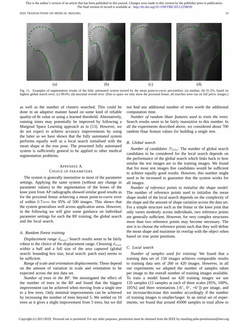
Fig. 11 shows various segmentation results of the fullyautomated system, ranked according to mean point-to-curvepercentiles: (a) gives the median result (50% of the imageshave a mean error of less than0.4mm); (b) is based onthe highest global search error yielding a mean segmentationerror of 0.6mm; (c) shows the 99%ile achieving an accuracyof 0.9mm; (d) gives the highest overall segmentation errorcorresponding to a mean error of2.7mm. These results showthat the global search had a success rate of100% in that itworked sufficiently well to initialise the local search.

A direct comparison to other reported automatic proximalfemur segmentation results is difficult as most findings areeither given qualitatively, or are not easy to interpret in moregeneral terms. The best reported results appear to be those byPilgram et al. [14] with a point-to-curve error of within1.6mm

for 80% of the 117 test cases (estimated on the basis of a likelyaverage shaft width of 209 pixels relative to the stated imagewidth of 2320 pixels).

The fully automated segmentation system was developedusing C++. All experiments were run on a 3.3 GHz Intel CoreDuo PC in a VMware using 2GB RAM. No parallel computingwas implemented. The global search took on average 15s perimage, and the local search 10s per image and cluster. For theresults in Section VI-C, we searched on average ten clusters.Note that running times vary depending on image size andsearch settings.

VII. D ISCUSSION AND CONCLUSIONS

We have presented a system to segment the proximalfemur in AP pelvic radiographs which is fully automatic,does not make any assumptions about the femur pose, andis very accurate.3 The segmentation system comprises twosteps, femur detection and femur segmentation, both of whichare based on a RF regression-based voting approach. For thesegmentation step, we incorporated the latter into the CLMframework.

We have shown that the system achieves excellent perfor-mance in both its steps when tested on a data set of 839 imagesof mixed quality. The femur detector, achieving an accuracyof a mean point-to-point error of less than8.4mm for 99%of all images, works sufficiently well to initialise the localmodel used for segmentation. This is also reflected in thefully automated system yielding equally high accuracy as alocal search initialised with the mean shape at correct pose,as seen by the overlapping plots in Fig. 7. In our experiments,the fully automatic segmentation system achieved an overallmean point-to-curve error of less than0.9mm for 99% of all839 images. We believe that this is the most accurate fullyautomatic system for segmenting the proximal femur in APpelvic radiographs so far reported.

In all the experiments above, the performance of the sys-tem depends on the random samples used to train the RFs.For different training sets, there will be a slight changein performance. However, our cross-validation experimentsdemonstrate that this difference is very small. For example,for the fully automatic system using a two-stage local searchmodel (as in Figure 7) the difference in medians betweenthe two single experiments (i. e. when switching the randomlyassigned training and test sets) is0.005mm.

In Appendix A, we discuss our choices of parameters andprovide guidance to their setting.

A limiting factor for higher accuracy is the quality of themanual annotation. This is not only because the manual anno-tation is used to train the models but also because using themanual annotation as ground truth for performance evaluationcan result in wrong error measurements. To estimate the intra-observer variability of the manual annotation, 20 images (10females and 10 males) where reannotated after a period of10 months. The difference in point-to-curve errors betweenthe intra-observer variability and the fully automated systemamounts to0.1mm for the medians and to0.2mm for the95%iles. Inter-observer variability is likely to be larger.

We have examined the performance of mixed-gender andgender-specific models showing that mixed-gender modelsperform well on male and female data sets. We thereforeconclude that there is no need to train gender-specific models.This is important when taking the segmentation system intopractice as it means that radiographs would not need to bepre-selected. It also allows aricher model as it can be trainedon a bigger mixed data set.

Overall the fully automated segmentation system is fast butfor applications where running time is crucial efficiency couldbe improved by adjusting the number of search iterations

3For access to the segmentation tool, please contact the authors.




(a) (b) (c) (d)

Fig. 11. Examples of segmentation results of the fully automated system (sorted by the mean point-to-curve percentiles): (a) median; (b) 91.2%, based onhighest global search error; (c) 99.0%; (d) maximal overall error. (Due to space we only show the proximal femur; all searcheswere run on full pelvic images.)

as well as the number of clusters searched. This could bedone in an adaptive manner based on some kind of reliablequality-of-fit value or using a learned threshold. Alternatively,running times may potentially be improved by following aMarginal Space Learning approach as in [13]. However, wedo not expect to achieve accuracy improvements by usingthe latter as we have shown that the fully automated systemperforms equally well as a local search initialised with themean shape at the true pose. The presented fully automatedsystem is sufficiently general to be applied to other medicalsegmentation problems.

APPENDIX ACHOICE OF PARAMETERS

The system is generally insensitive to most of the parametersettings. Applying the same system (without any change inparameter values) to the segmentation of the bones of theknee joint from AP radiographs showed similar good results asfor the proximal femur achieving a mean point-to-curve errorof within 0.7mm for 95% of 500 images. This shows thatthe system generalises well across application areas. However,in the following we will give some guidance on individualparameter settings for each the RF training, the global searchand the local search.

A. Random Forest training

Displacement rangedmax: Search results seem to be fairlyrobust to the choice of the displacement range. Choosingdmax

within a half and a full size of the area captured (globalsearch: bounding box size, local search: patch size) seems tobe sufficient.

Range of scale and orientation displacements: These dependon the amount of variation in scale and orientation to beexpected across the test data set.

Number of trees in the RF: We investigated the effect ofthe number of trees in the RF and found that the biggestimprovement can be achieved when moving from a single treeto a few trees. Only minimal improvements can be achievedby increasing the number of trees beyond 5. We settled on 10trees as it gives a slight improvement from 5 trees, but we did

not find any additional number of trees worth the additionalcomputation time.

Number of random Haar features used to train the trees:Search results seem to be fairly insensitive to this number.Inall the experiments described above, we considered about 700random Haar feature values for building a single tree.

B. Global search

Number of candidatesNfits: The number of global searchcandidates to be considered for the local search depends onthe performance of the global search which links back to howsimilar the test images are to the training images. We foundthat for most test images five candidates would be sufficientto achieve equally good results. However, this number mightneed to be increased to guarantee that the system works forall images.

Number of reference points to initialise the shape model:The number of reference points used to initialise the meanshape model of the local search depends on the complexity ofthe shape and the amount of shape variation across the data set.For a simple structure such as the femur or the knee joint thatonly varies modestly across individuals, two reference pointsare generally sufficient. However, for very complex structuresmore than two reference points may become necessary. Theaim is to choose the reference points such that they well definethe mean shape and maximise its overlap with the object whenbased on true point positions.

C. Local search

Number of samples used for training: We found that atraining data set of 150 images achieves comparable resultsto training data sets of 260 or 420 images. However, in allour experiments we adapted the number of samples takenper image to the overall number of training images available.To train a model based on 420 training images we use135 samples (15 samples at each of three scales [95%, 100%,105%] and three orientations [-6◦, 0◦, +6◦]) per image, andwe increase/decrease this number accordingly if the numberof training images is smaller/larger. In an initial set of exper-iments, we found that around 45000 samples in total allow to




achieve high accuracy with only slight accuracy improvementswhen using more.

Reference frame width: We chose the reference frame widthof the refinement modelto match the area captured (ROI) inour high resolution images such that for images where highresolution information is available no down sampling takesplace. The reference frame width of thebasis modelis morearbitrary but we recommend it to be between a quarter anda half of the reference frame width of therefinement model.The aim is that when down sampling your images so that thereference frame width of thebasis modelcorresponds to thewidth of the ROI the structures to be segmented should stillbe clearly visible.

Patch size: The patches need to be big enough to containstructural information that is relevant for the segmentation. Thepatches should cover a large enough area such that patches fordifferent landmarks are distinguishable; if necessary makinguse of structural information that is not part of the model (e. g.in our case the trochanters and pelvis). This is particularlyimportant for thebasis modelwhich may start searching fromfar off the true object contour. The patch size of therefinementmodelcan be smaller (with respect to the particular referenceframe width) as this model is expected to start searching fromvery close to the true answer – though the patches shouldbe big enough to capture the object contour as well as somebackground. Not that the patch size influences the runtime andsize of the model.

Search rangedsearch: For thebasis model, the search rangeshould be big enough to capture enough structural informationto be able to guide the model towards the object contour. In ourcase, we chosedsearch = 35 as this allows points along theshaft to include information about the lesser trochanter whichfor most of the shaft points is the only nearby structure thathas a distinguishable relative position to each of the points.For the refinement model, a rather small search range (withrespect to the particular reference frame width) is sufficient asthis model is expected to start searching from very close tothe true answer – therefinement modelis meant to only refinethe result and not to drift off the already found object contour.

Number of samples used to create response imagesR: In [7]we have shown that it is sufficient to sample the search rangeon a sparse grid. Across our experiments, we found a stepsize of 3 (i. e. to only take one sample in each 3x3 square) toachieve good accuracy while significantly increasing runtime.

Optimisation parameters for landmark updates: As de-scribed in Section III-B, we set the initial disk radius to matchsearch rangedsearch, rmin = 0.4 and the number of searchstepsk such thatdsearch∗0.6k ≤ rmin. The crucial point is toset the initial disk radius to equal the search range. The searchresults seem to be fairly insensitive to the choice ofrmin.

REFERENCES

[1] L. Breiman, “Random forests,”Machine Learning, vol. 45, pp. 5–32,2001.

[2] A. Criminisi, J. Shotton, D. Robertson, and E. Konukoglu,“Regressionforests for efficient anatomy detection and localization in CT studies,”in Medical Computer Vision Workshop. SpringerLecture Notes inComputer Science #6533, 2010, pp. 106–117.

[3] R. Girshick, J. Shotton, P. Kohli, A. Criminisi, and A. Fitzgibbon, “Ef-ficient regression of general-activity human poses from depth images,”in ICCV. IEEE Press, 2011, pp. 415–422.

[4] F. Schroff, A. Criminisi, and A. Zisserman, “Object Class Segmentationusing Random Forests,” inBMVC, 2008.

[5] J. Gall and V. Lempitsky, “Class-specific Hough forests for objectdetection,” inCVPR. IEEE Press, 2009, pp. 1022–1029.

[6] D. Ballard, “Generalizing the Hough transform to detectarbitraryshapes,”Pattern Recognition, vol. 13, no. 2, pp. 111–122, 1981.

[7] T. Cootes, M. Ionita, C. Lindner, and P. Sauer, “Robust and accurateshape model fitting using random forest regression voting,” in ECCV2012, To appear.

[8] D. Cristinacce and T. Cootes, “Automatic feature localisation withConstrained Local Models,”Journal of Pattern Recognition, vol. 41,no. 10, pp. 3054–3067, 2008.

[9] C. Lindner, S. Thiagarajah, J. Wilkinson, arcOGEN Consortium, G. Wal-lis, and T. Cootes, “Accurate fully automatic femur segmentation inpelvic radiographs using regression voting,” inMICCAI, 2012. Toappear.

[10] T. Cootes, C. Taylor, D. Cooper, and J. Graham, “Active Shape Models- Their training and application,”Computer Vision and Image Under-standing, vol. 61, no. 1, pp. 38–59, 1995.

[11] T. Cootes, G. Edwards, and C. Taylor, “Active Appearance Models,” inECCV. SpringerLecture Notes in Computer Science #1407, 1998, pp.484–498.

[12] G. Behiels, F. Maes, D. Vandermeulen, and P. Suetens, “Evaluation ofimage features and search strategies for segmentation of bonestructuresin radiographs using Active Shape Models,”Medical Image Analysis,vol. 6, no. 1, pp. 47–62, 2002.

[13] Y. Zheng, B. Georgescu, and D. Comaniciu, “Marginal Space Learningfor Efficient Detection of 2D/3D Anatomical Structures in MedicalImages,” inIPMI. SpringerLecture Notes in Computer Science #5636,2009, pp. 411–422.

[14] R. Pilgram, C. Walch, M. Blauth, W. Jaschke, R. Schubert,and V. Kuhn,“Knowledge-based femur detection in conventional radiographs of thepelvis,” Computers in Biology and Medicine, vol. 38, pp. 535–544, 2008.

[15] R. Smith, K. Najarian, and K. Ward, “A hierarchical methodbased onactive shape models and directed Hough transform for segmentation ofnoisy biomedical images; application in segmentation of pelvic x-rayimages,”BMC Medical Informatics and Decision Making, vol. 9, no.Suppl 1, pp. S2–S12, 2009.

[16] F. Ding, W. Leow, and T. Howe, “Automatic segmentation of femurbones in anterior-posterior pelvis x-ray images,” inCAIP. VerlagLecture Notes in Computer Science #4673, 2007, pp. 205–212.

[17] J. Canny, “A computational approach to edge detection,”IEEE Transac-tions on Pattern Analysis and Machine Intelligence, vol. 8, pp. 679–698,1986.

[18] S. Schulter, C. Leistner, P. Roth, L. V. Gool, and H. Bischof, “On-lineHough Forests,” inBMVC, 2011.

[19] P. Viola and M. Jones, “Rapid object detection using a boosted cascadeof simple features,” inCVPR. IEEE Press, 2001, pp. 511–518.

[20] C. Lindner, S. Thiagarajah, J. Wilkinson, arcOGEN Consortium, G. Wal-lis, and T. Cootes, “Short-term variability of proximal femurshapein anteroposterior pelvic radiographs,” inProceedings Medical ImageUnderstanding and Analysis, 2011, pp. 69–73.



Documents

Fully Automatic Segmentation of the Proximal Femur …Fully Automatic Segmentation of the Proximal ... CLM-based contour extraction yields a robust and fully auto- ... dependent on