Full-text Available Online at PRINT ISSN 1119-8362 https

*Corresponding Author Email: [email protected]

PRINT ISSN 1119-8362

ELECTRONIC ISSN 2659-1502

J. Appl. Sci. Environ. Manage.

Vol. 22 (12) 1917–1924 December 2018

Full-text Available Online at

https://www.ajol.info/index.php/jasem

http://ww.bioline.org.br/ja

Land Use/Land Cover Change Analysis using Markov-Based Model for Eleyele

Reservoir

BELLO, HO; *OJO, OI; GBADEGESIN, AS

Ladoke Akintola University of Technology, Ogbomoso, Nigeria

*Corresponding Author Email: [email protected]

ABSTRACT: Land Use and Land Cover (LULC) are important components of the environmental system and changes

in it mirror the impacts of human activities on the environment. These impacts needed to be determined in order to get a

clear picture of the extent at which different land use practices affect hydrologic regime and water quality. Therefore, this

study analyzed the effects of LULC on Eleyele reservoir for a period of 32 years. Landsat images of 1984, 2000 and 2016

covered by path 191 and rows 55 were acquired, a modified version of Aderson scheme of LULC classification was used

to stratify the images, while the LULC map was analyzed and projected until year 2032 using IDRISI Selva 17.0 and

ERDAS 2013 softwares respectively. Changes that have occurred within the study area were determined using LULC

MARKOV. Land Use Land Cover built up area increased from 688.30 ha to 952.68 ha and from 952.68 ha to 2164.5 ha

between years 1984 to 2000, and 2000 to 2016 respectively. LULC maps of 2000 and 2016 showed the open water also

reduced from 101.6 ha in year 2000 to 61.74 ha in 2016. DEM showed that 8.5%, and 1.9% transitioned to vegetation cover

and built up area in 1984 and 2000 respectively. Land Use Land Cover MARKOV chain analysis shows that by projection,

the reservoir area will reduce further to 39.08 ha by the year 2032. The study has established that reserved forest zone

suffered degradation with a noticeable increase in encroachment on the reservoir. LULC approach can be used to predict

the effect of land use on reservoirs.

DOI: https://dx.doi.org/10.4314/jasem.v22i12.8

Copyright: Copyright © 2018 Bello et al. This is an open access article distributed under the Creative

Commons Attribution License (CCL), which permits unrestricted use, distribution, and reproduction in any

medium, provided the original work is properly cited.

Dates: Received: 26 June 2018; Revised: 21 November 2018; Accepted 18 December 2018

Keywords: land use; land cover; analysis; model; Eleyele; reservoir

Land use is the intended employment of land

management strategy placed on the land cover by

human agents, or land managers to exploit the land

cover and reflects human activities such as industrial

zones, residential zones, agricultural fields, grazing,

logging, and mining among many others (Zubair,

2006; Chrysoulakis et al., 2004). According to

Quentin et al., (2006) land use change is defined to be

any physical, biological or chemical change

attributable to management, which may include

conversion of grazing to cropping, change in fertilizer

use, drainage improvements, installation and use of

irrigation, plantations, building farm dams, pollution

and land degradation, vegetation removal, changed

fire regime, spread of weeds and exotic species, and

conversion to non-agricultural uses. Land use and land

cover changes may be grouped into two broad

categories as conversion and modification.

Conversion refers to changes from one cover or use

type to another, while modification involves

maintenance of the broad cover or use type in the face

of changes in its attributes (Baulies and Szejwach,

1998). It is estimated that undisturbed (or wilderness)

areas represent 46% of the earth’s land surface. Forests

covered about 50% of the earth’s land area 8000 years

ago, as opposed to 30% today as agriculture has

expanded into forests, savannas, and steppes in all

parts of the world to meet the demand for food and

fiber (Lambin et al., 2003). Based on data from diverse

sources, the Global Forest Resources Assessment

2000 estimated that the world’s natural forests

decreased by 16.1 million hectares per year on average

during the 1990s, which is a loss of 4.2% of the natural

forest that existed in 1990 (Lambin et al., 2003). Land

use in East Africa has changed swiftly over the last

half-century: expansion of mixed crop-livestock

systems into former grazing land and other natural

areas and intensification of agriculture are the two

largest changes that have been detected (Olson and

Maitima, 2006). Accordingly, land cover

classification has recently been a hot research topic for

a variety of applications (Liang et al., 2002). A great

deal of research has been conducted throughout the

world in an attempt to understand major shifts in land

use and land cover and to relate them to changing

environmental conditions. Therefore, Land use and

land cover change (LULC) research needs to deal with

the identification, qualitative description and

parameterization of factors, which drive changes in

land use and land cover, as well as the integration of

Land Use/Land Cover Change Analysis….. 1918

BELLO, HO; OJO, OI; GBADEGESIN, AS

their consequences and feedbacks (Baulies and

Szejwach, 1998). However, one of the major

challenges in LULC analysis is to link behavior of

people to biophysical information in the appropriate

spatial and temporal scales (Codjoe, 2007).

Nevertheless, it is argued that land use and land cover

change trends can be easily accessed and linked to

population data, if the unit of analysis is the national,

regional, district or municipal level. LUCC studies

have been designed to improve understanding of the

human and biophysical forces that shape land use and

land cover change. Land use and land cover plays an

important role in global environmental change and

sustainability, including response to climate change,

effects on ecosystem structure and function, species

and genetic diversity, water and energy balance, and

agro-ecological potential. Land use and land cover

mapping is one of the most important and typical

applications of remote sensing data (Chrysoulakis et

al., 2004). Remotely sensed data are a useful tool, have

scientific value for the study of human environment

interactions, especially land use, and land cover

changes (Dale et al., 1993; Codjoe, 2007). Remote

sensing change detection techniques can be broadly

classified as either pre- or post-classification change

methods. A pre-classification process refers to

operations carried out to bring satellite images to the

desirable geometric and spectral standard by

correcting errors, and it is performed prior to image

classification. Research evaluating the comparative

performance of various land cover change detection

methods has indicated that no uniform combination of

data types and methods can be applied with equal

success across different ecosystems (Lu et al., 2004;

Lunetta et al., 2006). The study assessed the impact of

land use on Eleyele Water Reservoir, and evaluated

the relationship between the reservoir and the weather

parameters.

MATERIALS AND METHODS The Study Area: Eleyele Lake Forest is located in

Ibadan North West Local Government Area of Oyo

State, Nigeria. The forest lies within latitude 70 30’ –

70 45’ N and longitude 30 55’ – 30 88’ E. The study area

is surrounded by Eleyele neighborhood in the south,

Apete in the east and Awotan in the north. Eleyele

wetland is a modified natural riverine wetland type

with area of about 100 Km2 including the catchment

area. The elevation is relatively low ranging between

100-150 m above sea level and surrounded by quartz-

ridge hills toward the downstream section where the

Eleyele dam barrage is located. The total area of the

reserve is 526.0921 hectares and was originally

acquired by government under the public lands

acquisition ordinance in 1941 (Akingbogun, et al.,

2012), the reservoir was made by damming River Ona.

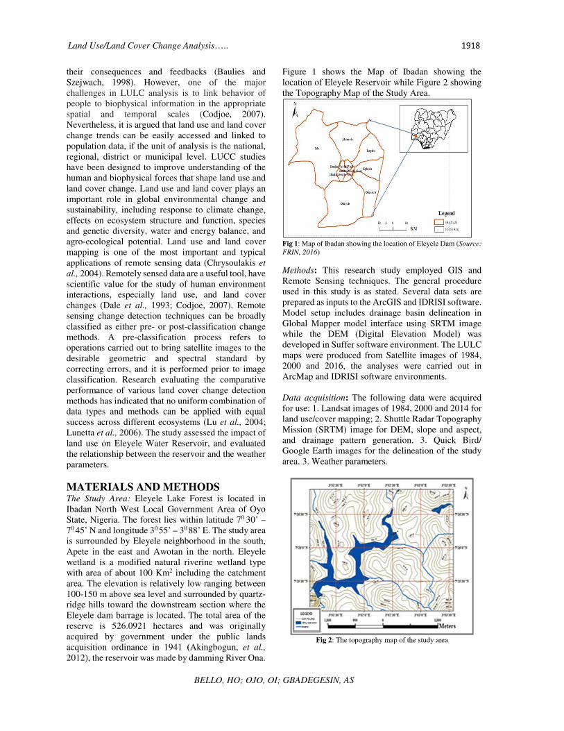
Figure 1 shows the Map of Ibadan showing the

location of Eleyele Reservoir while Figure 2 showing

the Topography Map of the Study Area.

Fig 1: Map of Ibadan showing the location of Eleyele Dam (Source:

FRIN, 2016)

Methods: This research study employed GIS and

Remote Sensing techniques. The general procedure

used in this study is as stated. Several data sets are

prepared as inputs to the ArcGIS and IDRISI software.

Model setup includes drainage basin delineation in

Global Mapper model interface using SRTM image

while the DEM (Digital Elevation Model) was

developed in Suffer software environment. The LULC

maps were produced from Satellite images of 1984,

2000 and 2016, the analyses were carried out in

ArcMap and IDRISI software environments.

Data acquisition: The following data were acquired

for use: 1. Landsat images of 1984, 2000 and 2014 for

land use/cover mapping; 2. Shuttle Radar Topography

Mission (SRTM) image for DEM, slope and aspect,

and drainage pattern generation. 3. Quick Bird/

Google Earth images for the delineation of the study

area. 3. Weather parameters.

Fig 2: The topography map of the study area



Data preparation: Land Use/Cover Map of Eleyele

basin was generated using Landsat 7TM and eight

ETM+ images covered by path 191, rows 55, these

satellite images were obtained as rectified data, and a

supervised classifier (parallelepiped classification)

was used to stratify the images. The land cover map

was analysed and projected using IDRISI Selva 17.0

and ERDAS 2013 software (Agbor et al., 2012). The

land use/cover classes considered were Forestland,

built-up area and water body.

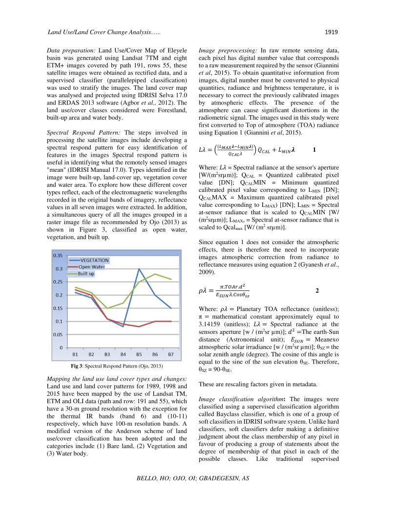
Spectral Respond Pattern: The steps involved in

processing the satellite images include developing a

spectral respond pattern for easy identification of

features in the images Spectral respond pattern is

useful in identifying what the remotely sensed images

"mean" (IDRISI Manual 17.0). Types identified in the

image were built-up, land-cover up, vegetation cover

and water area. To explore how these different cover

types reflect, each of the electromagnetic wavelengths

recorded in the original bands of imagery, reflectance

values in all seven images were extracted. In addition,

a simultaneous query of all the images grouped in a

raster image file as recommended by Ojo (2013) as

shown in Figure 3, classified as open water,

vegetation, and built up.

Fig 3: Spectral Respond Pattern (Ojo, 2013)

Mapping the land use land cover types and changes:

Land use and land cover patterns for 1989, 1998 and

2015 have been mapped by the use of Landsat TM,

ETM and OLI data (path and row: 191 and 55), which

have a 30-m ground resolution with the exception for

the thermal IR bands (band 6) and (10-11)

respectively, which have 100-m resolution bands. A

modified version of the Anderson scheme of land

use/cover classification has been adopted and the

categories include (1) Bare land, (2) Vegetation and

(3) Water body.

Image preprocessing: In raw remote sensing data,

each pixel has digital number value that corresponds

to a raw measurement required by the sensor (Giannini

et al, 2015). To obtain quantitative information from

images, digital number must be converted to physical

quantities, radiance and brightness temperature, it is

necessary to correct the previously calibrated images

by atmospheric effects. The presence of the

atmosphere can cause significant distortions in the

radiometric signal. The images used in this study were

first converted to Top of atmosphere (TOA) radiance

using Equation 1 (Giannini et al, 2015).

�� = �� + �� 1

Where: �� = Spectral radiance at the sensor's aperture

[W/(m2srµm)]; QCAL = Quantized calibrated pixel

value [DN]; QCALMIN = Minimum quantized

calibrated pixel value corresponding to LMIN [DN];

QCALMAX = Maximum quantized calibrated pixel

value corresponding to LMAX) [DN]; LMIN = Spectral

at-sensor radiance that is scaled to QCALMIN [W/

(m2srµm)]; LMAX, = Spectral at-sensor radiance that is

scaled to Qcalmax [W/ (m2 srµm)].

Since equation 1 does not consider the atmospheric

effects, there is therefore the need to incorporate

images atmospheric correction from radiance to

reflectance measures using equation 2 (Gyanesh et al.,

2009).

�� = �.�� .!"

#$% �.�&'()* 2

Where: �� = Planetary TOA reflectance (unitless);

π = mathematical constant approximately equal to

3.14159 (unitless); �� = Spectral radiance at the

sensors aperture [w / (m2sr µm)]; ,- =The earth-Sun

distance (Astronomical unit); ./0� = Meanexo

atmospheric solar irradiance [w / (m2sr µm)]; θSZ = the

solar zenith angle (degree). The cosine of this angle is

equal to the sine of the sun elevation θSE. Therefore,

θSZ = 90-θSE.

These are rescaling factors given in metadata.

Image classification algorithm: The images were

classified using a supervised classification algorithm

called Bayclass classifier, which is one of a group of

soft classifiers in IDRISI software system. Unlike hard

classifiers, soft classifiers defer making a definitive

judgment about the class membership of any pixel in

favour of producing a group of statements about the

degree of membership of that pixel in each of the

possible classes. Like traditional supervised



classification procedures, each uses training site

information for classifying each image pixel.

However, traditional hard classifiers output is not a

single classified land cover map, but rather, a set of

images (one per class) that expresses for each pixel the

probability that it belongs to each class (Giannini et al,

2015).

LULC change analysis using Markov- Based Model:

A raster data model in GIS (Markov-based) were used

to represent continuous data over space. The model

will divide the area into grid cells or pixels where each

grid cell were filled with the measured attribute values

in a matrix and cell values were written in rows and

columns. CA-Markov models represent, for example,

a forest area with lattice of cells, each of which exists

in one of a finite set of states.

The progression of time were modeled as a series of

discrete steps with future patterns determined by

transition rules, which specify the behavior of cells

over time, for example, a cell switches from forest area

to built-up area, as a function of conditions at each cell

and its neighboring cells at each time step (Giannini et

al, 2015). The pixel value of the raster data model in

classified images and the simulated images from CA-

Markov represents each land using land use and cover

change data derived from satellite images. This study

also established the validity of the Markov process for

describing and projecting land use and cover changes

in the study area by examining statistical

independence, Markovian compatibility, and the states

of the data as the Markov chain has n states. The data

vector is a column vector whose ith component

represents the probability that the system is in the ith

state at that time. It is important to note that the sum of

the entries of a state vector is 1; vectors X0 and X1 in

the above example are state vectors. If pij is the

probability of movement (transition) from one state j

to state i, then the equation 3 is called the transition

matrix of the Markov chain (Kampanart et al., 2016).

T = [pij] 3

The CA-Markov analysis was used to test run a pair of

land cover images and outputs a transition probability

matrix and a transition areas matrix. The transition

probability matrix explain the probability that each

land cover category changed to every other category.

The transition areas matrix is the number of pixels that

are expected to change from each land cover type to

every other land cover type over the specified number

of time units. Based on this a four-state markov

probability matrix has been developed (Takayama et

al., 1997).

Data Analysis: The analysis of data were carried out

using IDRISI, landsat image Google Earth and shuttle

radar topography mission (SRTM) softwares. Changes

that have occurred within then study area were

determined using a land use and land cover change

procedure called CA_MARKOV chain analysis. This

helped in correlating changes GPS for navigation and

recording of coordinates of landmark features.

RESULTS AND DISCUSSION The results are presented inform of images/maps,

graphs and statistical tables which include the land

cover types, change maps and land use land cover

transition maps and land use land cover types over the

study years.

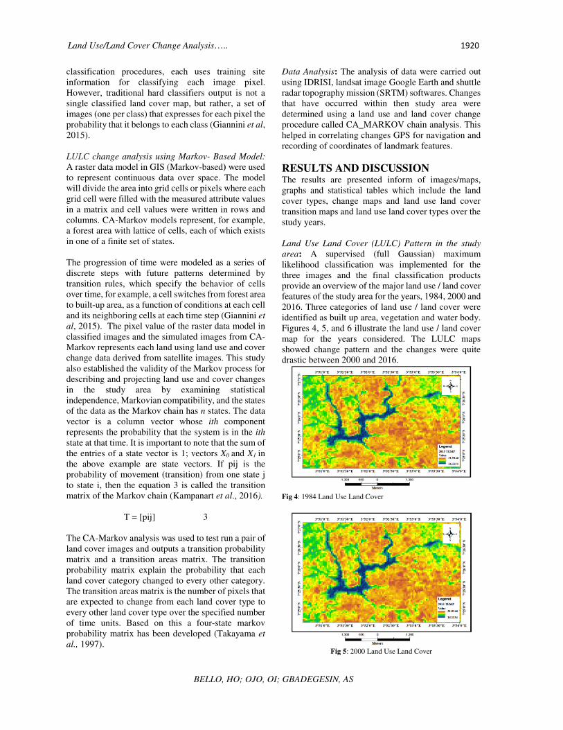
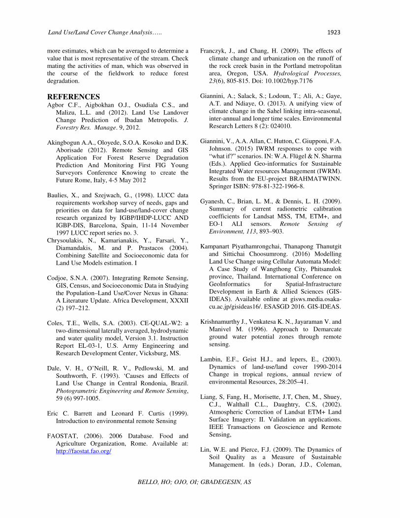
Land Use Land Cover (LULC) Pattern in the study

area: A supervised (full Gaussian) maximum

likelihood classification was implemented for the

three images and the final classification products

provide an overview of the major land use / land cover

features of the study area for the years, 1984, 2000 and

2016. Three categories of land use / land cover were

identified as built up area, vegetation and water body.

Figures 4, 5, and 6 illustrate the land use / land cover

map for the years considered. The LULC maps

showed change pattern and the changes were quite

drastic between 2000 and 2016.

Fig 4: 1984 Land Use Land Cover

Fig 5: 2000 Land Use Land Cover



Fig 6:2016 Land Use Land Cover

The statistics of LULC in 1984, 2000, 2016 and 2032

were stated in Tables 1 and 2. In order to obtain the

area extent (in hectares) of the resulting land use / land

cover type for each study year and for subsequent

comparison. Tables 1 and 2 showed the spatial extent

of land cover in hectares and in percentages, while

Figure 7 showed a dramatic increase in built area

between 2000 and 2016, it also indicates that both

water body and vegetation cover continued to

decrease. These results conformed to the study on land

use and land cover changes effects on human

environment interactions by Codjoe (2007).

Table 1: Land use Land Cover distribution pattern between 1984

and 2016

Table 2: 2032 LULC

Category 2032 Legend

Hectares %

1 2289.42 58.00 Built Up Area

2 54.54 1.39 Open Water

3 1564.92 40.03 Vegetation Cover

TOTAL 3908.88

Fig 7: Land cover types over the years (1984-2016) in Hectare

Fig 8: 2032 LULC Map

Land Use land Cover Projection using Markov

Operation: Markov chain analysis described land use

change from one period to another and used to project

future change. From Table 4, it is clear that the water

body / class is endangered because of the high

probability of it transitioning into built up area, the

area extent of the vegetation cover is likely to be taken

over by the built up area between 2000 and 2016.

These probabilities show serious threat faced by

Eleyele both now and the nearest future due to

anthropogenic activities. The decrease in open water

from 2.59% to 1.58% is a reflection of the given

statistics in Table 5.

Table 4: Markov: 2000/2016 Transition Probability of LULC

changes

LULC Built

Up

Open

Water

Vegetation

Cover

Built Up 0.6294 0.0116 0.3589 Open Water 0.5794 0.0472 0.3734

Vegetation Cover 0.5277 0.0158 0.4565

Table 5: 2032 Transition Table

Category 2032 Legend

Hectares %

1 2289.42 58.00 Built Up Area

2 54.54 1.39 Open Water

3 1564.92 40.03 Vegetation Cover

TOTAL 3908.88

Fig 9: 2000/2016 Change Map



Transition mapping: The change map (Figure 9)

shows how land cover types transitioned to other types

between 1984 and 2000. For example, 8.5% of

vegetation in 1984 transitioned to built-up area in

2000, while 1.9% of built up area transitioned to

vegetation area denoting change statistics shown in

Table 6.

Table 6: Change map statistics

Category Hectares % Legend

1 330.9918750 8.47 vegetation cover

to built up area

2 18.9254250 0.48 vegetation cover

to open water

3 76.7576250 1.96 built up area to

vegetation cover

4 28.4287500 0.73 open water to

vegetation cover

Fig 10: Gains and Losses of land use land cover type between

1984 and 2000

The gains and losses graph (Figure 10) reveals the

drastic decrease in vegetation cover and large increase

in built up area, between 1984 and 2000. The gains and

losses of the land cover types between 1984 and 2000

are shown in Figure 10, with vegetation losing more to

other land types by about 8.5%. The findings human

activities as one of the major challenges in LU-LC

analysis in the appropriate spatial and temporal scales

(Codjoe, 2007, Ojo, 2013).

Table 7: Transitions for LULC

Category Hectares Legend

1 611.5430250 1/1

3 330.9918750 3/1

5 94.6271250 2/2

6 18.9254250 3/2

7 76.7576250 1/3

8 28.4287500 2/3

9 2747.9229750 3/3

Note: 1-built up area, 2-open water and 3-vegetation cover

Cross-Classification: Cross-classification performed

using CROSSTAB module in IDRISI through analysis

that compares images containing categorical variables

of two types. For the first type used in this study,

which is hard classification, all pixels in the maps have

complete membership to exactly one category

resulting into a cross-classification image and table as

outputs. Olga et al., (2013) study in assessing spatial

dynamics of urban growth using an integrated land use

model agreed to the results in Table 7, Figures 11 and

12 depicting the built up area, open water and

vegetation cover dynamics.

Fig 11: Image cross-classification between 1984 and 2000

Fig 12: Image cross-classification between 2000 and 2016

Conclusion: The 1984, 2000 and 2016 Landsat

TM/OLI satellite data were used to identify and

classify LULC types of the study area as a GIS

database of land use categories and their location

within 32 years (1984-2016) was generated and

analyzed with the aid of GIS analytical functions. The

results showed that urban growth (anthropogenic

factors) within the study area imposes a lot of pressure

on the reservoir. Between 1984 and 2016, the depth of

the reservoir reduced significantly. By considering the

LULC maps of 2000 and 2016 shows how drastic the

reservoir as decreased from 101.6 ha in 2000 to 61.74

ha in 2016 which amount to 39.08 ha. The reserved

forest zone has suffered degradation seriously and if

the similar trend continues, the encroachment will

further reduce the reservoir area and the surrounding

reserved forest will disappear. By projection, the

reservoir area will reduce by 1% (39.08 ha) of the total

area considered for the study area by the year 2032.

More image cross-sections should be used to derive



more estimates, which can be averaged to determine a

value that is most representative of the stream. Check

mating the activities of man, which was observed in

the course of the fieldwork to reduce forest

degradation.

REFERENCES Agbor C.F., Aigbokhan O.J., Osudiala C.S., and

Malizu, L.L. and (2012). Land Use Landover

Change Prediction of Ibadan Metropolis. J.

Forestry Res. Manage. 9, 2012.

Akingbogun A.A., Oloyede, S.O.A. Kosoko and D.K.

Aborisade (2012). Remote Sensing and GIS

Application For Forest Reserve Degradation

Prediction And Monitoring First FIG Young

Surveyors Conference Knowing to create the

Future Rome, Italy, 4-5 May 2012

Baulies, X., and Szejwach, G., (1998). LUCC data

requirements workshop survey of needs, gaps and

priorities on data for land-use/land-cover change

research organized by IGBP/IHDP-LUCC AND

IGBP-DIS, Barcelona, Spain, 11-14 November

1997 LUCC report series no. 3.

Chrysoulakis, N., Kamarianakis, Y., Farsari, Y.,

Diamandakis, M. and P. Prastacos (2004).

Combining Satellite and Socioeconomic data for

Land Use Models estimation. I

Codjoe, S.N.A. (2007). Integrating Remote Sensing,

GIS, Census, and Socioeconomic Data in Studying

the Population–Land Use/Cover Nexus in Ghana:

A Literature Update. Africa Development, XXXII

(2) 197–212.

Coles, T.E., Wells, S.A. (2003). CE-QUAL-W2: a

two-dimensional laterally averaged, hydrodynamic

and water quality model, Version 3.1. Instruction

Report EL-03-1, U.S. Army Engineering and

Research Development Center, Vicksburg, MS.

Dale, V. H., O’Neill, R. V., Pedlowski, M. and

Southworth, F. (1993). ‘Causes and Effects of

Land Use Change in Central Rondonia, Brazil.

Photogrametric Engineering and Remote Sensing,

59 (6) 997-1005.

Eric C. Barrett and Leonard F. Curtis (1999).

Introduction to environmental remote Sensing

FAOSTAT, (2006). 2006 Database. Food and

Agriculture Organization, Rome. Available at:

http://faostat.fao.org/

Franczyk, J., and Chang, H. (2009). The effects of

climate change and urbanization on the runoff of

the rock creek basin in the Portland metropolitan

area, Oregon, USA. Hydrological Processes,

23(6), 805-815. Doi: 10.1002/hyp.7176

Giannini, A.; Salack, S.; Lodoun, T.; Ali, A.; Gaye,

A.T. and Ndiaye, O. (2013). A unifying view of

climate change in the Sahel linking intra-seasonal,

inter-annual and longer time scales. Environmental

Research Letters 8 (2): 024010.

Giannini, V., A.A. Allan, C. Hutton, C. Giupponi, F.A.

Johnson. (2015) IWRM responses to cope with

“what if?” scenarios. IN: W.A. Flügel & N. Sharma

(Eds.). Applied Geo-informatics for Sustainable

Integrated Water resources Management (IWRM).

Results from the EU-project BRAHMATWINN.

Springer ISBN: 978-81-322-1966-8.

Gyanesh, C., Brian, L. M., & Dennis, L. H. (2009).

Summary of current radiometric calibration

coefficients for Landsat MSS, TM, ETM+, and

EO-1 ALI sensors. Remote Sensing of

Environment, 113, 893–903.

Kampanart Piyathamrongchai, Thanapong Thanutgit

and Sittichai Choosumrong. (2016) Modelling

Land Use Change using Cellular Automata Model:

A Case Study of Wangthong City, Phitsanulok

province, Thailand. International Conference on

GeoInformatics for Spatial-Infrastructure

Development in Earth & Allied Sciences (GIS-

IDEAS). Available online at gisws.media.osaka-

cu.ac.jp/gisideas16/. ESASGD 2016. GIS-IDEAS.

Krishnamurthy J., Venkatesa K. N., Jayaraman V. and

Manivel M. (1996). Approach to Demarcate

ground water potential zones through remote

sensing.

Lambin, E.F., Geist H.J., and lepers, E., (2003).

Dynamics of land-use/land cover 1990-2014

Change in tropical regions, annual review of

environmental Resources, 28:205–41.

Liang, S, Fang, H., Morisette, J.T, Chen, M., Shuey,

C.J., Walthall C.L., Daughtry, C.S, (2002).

Atmospheric Correction of Landsat ETM+ Land

Surface Imagery: II. Validation an applications.

IEEE Transactions on Geoscience and Remote

Sensing,

Lin, W.E. and Pierce, F.J. (2009). The Dynamics of

Soil Quality as a Measure of Sustainable

Management. In (eds.) Doran, J.D., Coleman,



D.C., Bezdicek, D. F., Lunetta, R.L., Knight, F.K,

Ediriwickrema, J., Lyon, J.G., and Worthy, L.D.,

2006. Land covers change detection using multi-

temporal MODIS NDVI data. Remote Sensing of

Environment, 105, 142-154.

Lu, D., Mausel, P., Brondizio, E., and Moran, E.

(2004). Change detection techniques. Int. J.

Remote Sensing, 20(12), 2365-2407.

Lunetta, R.L., Knight, F.K, Ediriwickrem A, J., Lyon,

J.G., and Worthy, L.D., (2006). Land cover change

detection using multi-temporal MODIS NDVI

data. Remote Sensing of Environment, 105, 142-

154.

Ojo, O. I. (2013). Mapping and modeling of irrigation

induced salinity in Vaal Harts Irrigation scheme,

South Africa: a DTech Thesis submitted to the

Department of Civil Engineering, Tshwane

University of Technology, Pretoria, South Africa.

Olga Lucia Puertas, Cristian Henríquez and Francisco

Javier Meza. (2013). Assessing spatial dynamics of

urban growth using an integrated land use model.

Application in Santiago Metropolitan Area, 2010–

2045. Land Use Policy, 38(2014), 415–425.

Olson, Jennifer M., Bilal Butt, Fred Atieno, Joseph

Maitima, Thomas A. Smucker, Eric Muchugu,

George Murimi, and Hong Xu. 2004. Multi-scale

analysis of land use and management changes on

the Eastern Slopes of Mt. Kenya. Nairobi:

International Livestock Research Institute.

Quentin F. B., Jim, C., Julia, C., Carole, H., and

Andrew, S., (2006). Drivers of land use change,

Final report: Matching opportunities to

motivations, ESAI project 05116, Department of

Sustainability and Environment and primary

industries, Royal Melbourne Institute of

Technology. Australia.

Takayama S, Bimston DN, Matsuzawa S, Freeman

BC, Aime-Sempe C, Xie Z, Morimoto RJ and

Reed JC (1997) Bag-1 modulates the chaperone

activity of hsp70/hsc70. EMBO J 16: 4887–4896.

Zubair, A. O., 2006. Change detection in land use and

Land cover using remote sensing data and GIS (A

case study of Ilorin and its environs in Kwara

State), M.sc Thesis, University of Ibadan, Nigeria.

Documents

Full-text Available Online at PRINT ISSN 1119-8362 https