Full Matching in an Observational Study of Coaching for the SAT

Full Matching in an Observational Study of Coaching for the SATAuthor(s): Ben B. HansenSource: Journal of the American Statistical Association, Vol. 99, No. 467 (Sep., 2004), pp. 609-618Published by: American Statistical AssociationStable URL: http://www.jstor.org/stable/27590435 .

Accessed: 16/06/2014 11:47

Your use of the JSTOR archive indicates your acceptance of the Terms & Conditions of Use, available at .http://www.jstor.org/page/info/about/policies/terms.jsp

.JSTOR is a not-for-profit service that helps scholars, researchers, and students discover, use, and build upon a wide range ofcontent in a trusted digital archive. We use information technology and tools to increase productivity and facilitate new formsof scholarship. For more information about JSTOR, please contact [email protected].

.

American Statistical Association is collaborating with JSTOR to digitize, preserve and extend access to Journalof the American Statistical Association.

http://www.jstor.org

This content downloaded from 195.34.79.192 on Mon, 16 Jun 2014 11:47:12 AMAll use subject to JSTOR Terms and Conditions

http://www.jstor.org/action/showPublisher?publisherCode=astata

http://www.jstor.org/stable/27590435?origin=JSTOR-pdf

http://www.jstor.org/page/info/about/policies/terms.jsp


Full Matching in an Observational Study of

Coaching for the SAT Ben B. Hansen

Among matching techniques for observational studies, full matching is in principle the best, in the sense that its alignment of comparable treated and control subjects is as good as that of any alternate method, and potentially much better. This article evaluates the practical

performance of full matching for the first time, modifying it in order to minimize variance as well as bias and then using it to compare coached and uncoached takers of the SAT. In this new version, with restrictions on the ratio of treated subjects to controls within matched

sets, full matching makes use of many more observations than does pair matching, but achieves far closer matches than does matching with k>2 controls. Prior to matching, the coached and uncoached groups are separated on the propensity score by 1.1 SDs. Full matching reduces this separation to 1% or 2% of an SD. In older literature comparing matching and regression, Cochran expressed doubts that any

method of adjustment could substantially reduce observed bias of this magnitude. To accommodate missing data, regression-based analyses by ETS researchers rejected a subset of the available sample that differed

significantly from the subsample they analyzed. Full matching on the propensity score handles the same problem simply and without

rejecting observations. In addition, it eases the detection and handling of nonconstancy of treatment effects, which the regression-based

analyses had obscured, and it makes fuller use of covariate information. It estimates a somewhat larger effect of coaching on the math score

than did ETS's methods.

KEY WORDS: Graph algorithm; Matching with multiple controls; Network flow; Optimal matching; Quasiexperiment; Propensity score.

1. Introduction

During the 1995-1996 academic year, investigators from the

College Board surveyed a random sample of high school ju nior and senior SAT takers to probe how they had prepared for the SAT, asking whether they had completed extracurricular test

preparation courses, among other questions. Some 12% of re

spondents said that they had; the comparison of these to the

remaining 88% comprised the observational study reported by Powers and Rock (1999).

Powers and Rock estimated coaching effects in several ways, most of which started from regression models and one of which

involved matching. Matching was not their favorite approach:

"By its nature," they lamented, matching "significantly reduces

sample sizes," noting that their matched-pairs analysis matched

only a fraction of the uncoached students to coached coun

terparts (1999, p. 99). Their disappointment seemed to extend

from pair matching to matching in general, although it is not

clear that it should have. As compared to 1 : k matching or

to matching with a variable number of controls (Ming and

Rosenbaum 2000), pair matching is the least flexible and the

least able to make use of a large reservoir of potential controls.

This article revisits Powers and Rock's matching problem

using the most flexible approach applicable to it, namely op timal full matching (Rosenbaum 1991). Section 2 explains full

matching and contrasts it with pair matching and similar de

signs. Full matching remedies the sample reduction problem,

using all of the available sample, as none of Powers and Rock's

preferred adjustments was able to do; simultaneously, it pro

duces closer matches than do their methods. It turns out that

full matching is in a sense too flexible (Sec. 2.4); Section 3 ad

dresses this by modifying the technique to incorporate certain

restrictions. Full matching, either with or without restrictions,

Ben B. Hansen is Assistant Professor, Statistics Department, University of Michigan, Ann Arbor, MI 48109-1092 (E-mail: [email protected]; URL: www.stat.lsa.umich.edu/~bbh). The author thanks Paul R. Rosenbaum, as well as Luke Bulman, Tanya Henneman, Elizabeth A. Stuart, Yu Xie, and two anonymous referees for very helpful suggestions. He wishes to acknowl

edge the College Board, Donald E. Powers, and Donald A. Rock for graciously sharing the data from their SAT coaching study, Paul W. Holland for his kind

encouragement and for his help in obtaining the data, and the National Science

Foundation for material support (Postdoctoral Fellowship DMS-01-02056).

does a better job with missing data, facilitates fully adjusted but simple comparisons of treated and control groups, and lays bare heterogeneities of treatment effect that regression analyses

obscured.

The context of Powers and Rock's study was as follows.

The Princeton Review has long claimed its students' average benefit to be 140 points in combined SAT score (Princeton Review 2004), and during the 1990s Kaplan Educational Cen

ters claimed average benefits of 120 points (Zehr 2001). The

coaching companies' figures appear to be based on studies con

ducted for them by outside firms (Princeton Review 2004); but

because neither the studies nor methodological descriptions of

them are published or publicly available, the integrity of their

conclusions is difficult to assess. In contrast, Powers and Rock

found much weaker coaching effects: about 20 points on the

math section and 10 on the verbal. Their analyses assumed,

among other things, constancy of coaching effects. Granting

this and other premises, Powers and Rock's findings sharply refute those of the coaching companies. Section 4 will offer

strong evidence against uniformity of coaching effects, how

ever. Our full matching-based estimation of coaching effects, also presented in Section 4, relaxes this and others of Powers

and Rock's assumptions, yielding new evidence on the College Board's and the coaching companies' competing claims. Sec

tion 5 abstracts from the coaching study to discuss matching for observational studies in general.

1.1 Test Scores and Test Preparation in

a National Sample

The data to be analyzed derive from a stratified random sam

ple of registrants for 1995-1996 administrations of the SAT-I

test, details of which are given by Powers and Rock (1999). About 6,700 high school juniors and seniors received surveys

asking whether and how they had prepared for the test; the

replies of some 4,200 respondents were linked to the College Board's records of their scores on the 1995 or 1996 exams, as

? 2004 American Statistical Association

Journal of the American Statistical Association

September 2004, Vol. 99, No. 467, Applications and Case Studies

DOI 10.1198/016214504000000647

609



610 Journal of the American Statistical Association, September 2004

Table 1. Selected Pretreatment Variables

Variable Range of

values

Standardized

bias Percentage

of sample

Math section

of PSAT

Mean SAT at

respondent's first-choice

college

Father's

education

Average math grade

Foreign

language years taken

20-43

45-51

52-57

58-80

Not taken

787-987

988-1,060

1,061-1,123

1,124-1,336 No response

High school A.A. or B.A.

Graduate

No response

"Excellent"

"Good"-"fail"

No response

0-2

3-4

No response

18

17

16

15

34

16

16

16

16

36

40

26

25

9

35

59

6

64

27

9

well as scores on previous SAT-I or PSAT tests and their an

swers to the Student Descriptive Questionnaire (SDQ), which

all SAT-I registrants are asked to complete. By their responses to questions about extracurricular SAT preparation, respondents

split into a treated and a control group, and the data describe the

results of a classical quasiexperiment (Campbell and Stanley

1966). Nineteen in twenty of the survey respondents actually took

the spring 1996 or fall 1995 exam for which they had registered. The analysis given below restricts itself to these 3,994 stu

dents, using the corresponding SAT scores as outcome mea

sures. Thus the record gives coaching status and SAT outcomes

for all students in the sample to be analyzed; among the ad

ditional measures, each available for some fraction of the stu

dents, are pretest scores, racial and socioeconomic indicators,

various data about their academic preparation, and responses

to a survey item that, by eliciting students' first choices in col

leges, recovered an unusually discriminating measure of stu

dents' educational aspirations. In all, there are 27 pretreatment

variables.

The coached and uncoached groups differ appreciably in

these recorded measures?as do high and low scorers on the

SAT. Table 1 offers some illustration of this, giving over

all incidences of various covariate attributes and comparing their relative incidences in the coached and uncoached groups.

(The statistic here used to effect these comparisons is the stan

dardized bias, given for a variable v by (vt ?

vc)/sp, where

vt and vc are the average values of v in the treatment and control

groups, respectively, and s2 is the pooled within-group variance

in v.) Yet the table shows only five covariates; the analysis must

address biases on all 27 of them.

1.2 Missing and Misleading Data in Regression and in Subclassification

In regression-based adjustment, the simplest way to handle

missing data on a covariate is to reject cases without complete

information. In adjustment based on matching or stratification,

the method of first resort is to merge "missing" with an appro

priate level of the covariate, or to treat it as a category unto

itself. Thus missingness becomes part of the profiles according to which study subjects are sorted into strata or matched sets.

Good stratifications, then, will tend to group subjects that are

comparable in terms both of observed covariate values and of

covariate missingness.

Powers and Rock's (1999) study follows the norms of re

gression analysis rather than of stratification, rejecting all cases

with missing covariate values. Of the seven statistical analyses

they report having done, one used about an eighth of the avail

able sample, three more used about half, another two used three

quarters, and only one, the so-called "Belson model," used more

than 90% of it. The Belson model was an outlier in another re

spect: Its estimate of the effect of coaching on math scores was

closer to 30 points than the 15 or 20 found in the other analy ses. And the difference of the treated and control groups' mean

SAT scores is greater for the whole of the sample (41 ? 5 for

SAT-M, 9 ? 5 for SAT-V; n = 3,994) than for the half of the

sample used by three of Powers and Rock's analyses (35 ? 7

for SAT-M, 6 ? 7 for SAT-V; n = 1,876). The partly missing observations are decidedly unlike a randomly selected subset of

the sample; to the contrary, their removal from an the analysis

is likely to bias the result.

To illustrate how a stratification-based analysis might begin to address this problem, consider simple stratifications along the one or two covariates that most threaten to confound the

comparison of treated subjects to controls. With the College Board coaching data, race and socioeconomic status (SES) variables best fit this description. The one race variable sorts

subjects into eight ethnic categories, with only 6% of obser

vations missing. Several of these groups are quite small, and

collapsing seems in order. Given the education setting of the

study, it is natural (1) to sort observations into an Asian

American category (9%), an underrepresented minority cate

gory (8% Black, 3% Mexican American, 1% Native American, 1% Puerto Rican, 3% other Hispanic, 3% other), and White

(66%); and (2) to place the small fraction of item nonrespon dents with the largest category, namely White. To account for

SES, SDQ responses give three potential stratifiers to choose

from among, namely parents' income and education levels of

mothers and fathers. All three variables are probably measured

with some error, but it seems that high school students are more

likely to know and less likely to misreport their parents' ed

ucation than their parents' income; and splitting the data into

thirds at the 33%, 67%, and 100% quantiles of mother's and

of father's education levels, father's education better separates

both PSAT-math and PSAT-verbal scores. We stratify the Col

lege Board coaching data by race and father's education level,

grouping students into three categories of father's education,

plus an additional category for students not reporting it. Call

this the Race-by-SES (Race x SES) subclassification; Table 2

shows sizes and compositions of its subclasses.

The Race x SES subclassification adjusts for too few of

the available covariates to be taken seriously as an adjustment

unto itself, but it should be noted that it makes a promising

beginning. For instance, the association between PS AT math scores (grouped as in Table 1) and coaching status is signif icant at the .05 level in the unstratified sample, but not in



Hansen: Full Matching in an Observational Study 611

Table 2. Race x SES Subclasses: Sizes and

Control-to- Treated-Subject Ratios

Father's education Percentage Number of controls

(by race category) of sample per treated subject

White, or no race reported

High school or less 26 21 A.A. or B.A. 20 10

Postcollege 20 4.5 Not reported 7 4.5

White (all) 72 8.2

Underrepresented minority High school or less 11 11 A.A. or B.A. 3 6.6

Postcollege 3 3.6 Not reported 1 4.4

Underrepresented 19 7.2 minority (all) Asian American

High school or less 4 3.8 A.A. or B.A. 3 3.4

Postcollege 3 1.5 Not reported .4 15

Asian American (all) 9 2.9 All 100 7.0

the stratified sample, when evaluated with the Mantel (1963) score statistic; and after but not before subclassification along race and SES, a Cochran-Mantel-Haenszel test (Agresti 1990, sec. 7.4.6) fails to find significant differences between coached and uncoached students in terms of number of semesters taken

of high school English and natural science, English and natural science grades, and grades in social science and math courses.

Because other variables, such as overall high school grade point average (GPA) and reported parents' income, do not become balanced after stratification on SES and race, the analyst must

make one or more additional adjustments taking the remaining covariates explicitly into account. To effect such an adjustment,

Sections 3 and 4 of this article refine rather than replace the Race x SES subclassification, thus inheriting its gains.

Subclassifying in this way, we have rejected no observations.

Placing subjects with partially missing data into subclasses ded icated to their missingness pattern, as we have done, can solve

the missingness problem only if the unavailable covariate data are missing at random given those data that are not missing; but for the analogous strategy in regression contexts, namely case

wise deletion, it is necessary that the observations with partial missingness be like a simple random subsample of the sample as a whole?which in the present case appears not to be true.

The strategy of creating missingness levels of covariates can

also be used to construct propensity scores. It leads to propen

sity scores which, when matched or stratified upon, balance

both covariate-missingness and observed-covariate profiles be

tween treated and control groups (Rosenbaum and Rubin 1984,

app.); it is well-suited to missingness patterns in which obser vations tend to lack only few of a large number of covariates. Such is the case here: On the 23 covariates other than pretest scores, only one third of the College Board sample have com

plete data, but two thirds are missing no more than two covari

ates, and nine tenths lack data on no more than six covariates.

Our propensity score accommodates missing data in this way,

in so doing retaining all 3,994 observations.

Adjustment by stratification encourages the analyst to focus on the data rather than a model for it, and this can be indirectly beneficial. With these data, for example, there is a temptation to

regard as a pretreatment variable any PS AT or SAT score from a test sitting earlier than that of the posttest, in order to maximize

sample size in a regression using pretest scores as covariates; re

cent regression-based studies of coaching for the SAT share in such a simplifying assumption (Briggs 2001; Powers and Rock

1999). But as it turns out, in the College Board's sample there are quite a few coached students who got their coaching even

before taking their earliest SAT or PSAT: of 332 coached stu

dents reporting the years and months in which their test prepa ration courses began, one fourth started their courses before

taking either the SAT or the PSAT. Treating as pretests prior test scores that did not genuinely precede the treatment, as Briggs' and Powers and Rock's studies do, may deny credit to coach

ing programs for gains that they produced. (For a more general discussion of this point, see Rosenbaum 1984.) The analysis to follow treats the 126 coached students with prior tests that did not precede their coaching, or could not be determined to

have preceded it, the same as students without pretests: In re

fashioning the covariates for inclusion in a propensity score

model, they are placed in a "pretest-missing" category. To en

hance comparability of the groups, a similar accommodation is

made with uncoached students: Those who have prior tests that

only preceded their posttests by a period of less than 6 months are placed into a "pretest-missing" category, rather than a cate

gory based on groupings of pretest scores.

2. CONVENTIONAL MATCHING AND ALTERNATIVES

2.1 Nearest Available versus Optimal Matching

Most commonly, matchings join each treated subject to one or to a fixed number k > 2 of controls, and usually this match

ing is done by a so-called nearest available algorithm. Sec

tion 2.2 explores ramifications of matching treated and control

subjects in only one, preset ratio. As a prelude to that discus

sion, this section reviews the distinction between optimal and nearest available matching.

Table 3 presents an artificial dataset modeled on an unpub lished gender equity study conducted by the author. Men and

women university scientists within various departments were to

be compared in terms of their lab space assignments, but first it was necessary to match them on factors that might confound

the comparison. The actual study matched on total grant fund

ing and several other factors, but to simplify the illustration we

consider grant funding alone.

Nearest available, or greedy, matching algorithms move

down the list of treated subjects from top to bottom, at each

Table 3. A Gender Equity Matching Problem: Women and Men

Scientists Are to Be Matched on Grant Funding

Women Men

Subject log-?o (grant funding) Subject log:i o (grant funding) A 5.7 V 5.5

B 4.0 W 5.3 C 3.4 X 4.9

D 3.1 Y 4.9

Z 3.9




step matching a treated subject to the nearest available control,

which is then removed from the list of controls available at the next step. Matchings are made at a given stage without attention

to how they affect possibilities for later matchings. In the equity

matching problem posed in Table 3, a nearest available algo rithm for pair matching would first match A to V, then B to Z,

C to X, and finally D to Y, for a total "cost" (sum of absolute dif

ferences in log Grant Funding) of 3.6. Having matched A to V, Z is the nearest available potential match for B, but matching B to Z is in fact "greedy," in that it forces C and/or D to be more

poorly matched at the next stage. In contrast, optimal matching

algorithms optimize global, rather than local, objectives. The

optimal solution for the problem of pairing each of Table 3's women with one of its men joins A to V, B to X, C to Y, and

D to Z, for a total cost of 3.4.

For pair matching with a large reservoir of controls, greedy

algorithms often do nearly as well as optimal algorithms (Rosenbaum and Rubin 1985). But absent an excess of avail

able controls, or with unfortunate orderings of the list of treated

subjects, greedy algorithms can do much worse than optimal ones.

2.2 The Weakness of Fixed-Ratio Matching: Using More Controls Leads to Larger Biases

Returning to the coaching study, let us match coached and

uncoached students first as pairs, and then in fixed proportions 1 : k, letting k grow until all controls have been matched, and let

us compare these alternative matchings to one another. Because

optimal matches are never worse, and often better, than greedy

matches, we generate each match using optimal methods.

Surely the best 1:1 match is less likely than any 1 : k match, k > 2, to join a treated subject to a control that differs apprecia

bly from it; and surely it follows that among all 1 : k matches, k> 1, an optimal 1:1 match most reduces the bias of treatment

to control group comparisons. Yet it would be rash to prefer 1:1 matches categorically, because when more than one good

potential match is available for each treated subject, there will

be k > 2 such that some 1 : k match leads to sharper estimates

than do 1 : 1 matches, with little penalty in terms of bias. In the context of our coaching study, how much precision does each

increment to the number of controls buy, and at what cost in

terms of bias?

To appreciate the impact of the number of controls on the ef

fect estimate's variability, consider that estimate in the context

of a simple linear model. Attach numbers 1,..., n to sample

units; let T and C be the indices of the treated and the control

group, respectively, so that TUC = {l,...,n) and TflC =

0,

and let S indicate a partition of the sample into matched and

unmatched sets by mapping indices {1,..., n] of sample units to 0, for unmatched units, or to positive integers {1,..., S} in

dicating matched sets. (The 5th matched set, 1 < s < S, is then

represented as S-1 [s].) Then the model represents responses of

matched units [i for which S(z) > 0] as follows:

? rS(,-) + As(/) + Si, ieT

lAS(/)+e/, ieC,

E(?) = 0, Cov(?:) = cr2I, a2 < co, (1)

where Ai,..., A5 are matched-set effects and ri,..., T5 are

treatment-control contrasts, one for each matched set.

Under model (1), in the sth matched set the average differ ence of treatment- and control-subgroup responses, yst

? ysc,

unbiasedly estimates rs, and weighted averages J2 wsTs (w > 0,

]T ws = 1 ) may be estimated with weighted averages of these

matched-set response differences, J2ws^s- Given candidate

stratifications S : {0,..., n] -> {0,..., S} and S : {0,..., n) ?>

{0,..., S) with weightings w and w, therefore, the quotient

r(s,s)J?^_,#(S"'M) , V/2 \~[ #(Tns-l[s]).#(Cns-l[s])J

ns~l[s]) \ 2) 5=1 #(Tns^[~s]).#(Cns-i[s])/

[#(A) ?

size or cardinality of A] assesses the relative precision of estimates based on S and on S. When S and S give rise to

models of form (1) sharing a common value of a, R(S, S) is

the ratio of SD's of estimates of w- and w- weighted averages of

stratum treatment/control contrasts.

Comparisons based on this quotient favor 1 : k matchings with larger values of k. Weighting strata in proportion to the

number of treated subjects they contain is sometimes called

effect of treatment on the treated (ETT) weighting; using ETT weights, ws =

#({/ e T : S(z) = s})/#({i e T : S(i) > 0}),

and comparing each matching to a 1:1 matching, the relative

precision quotients for 1:1, 1:3, 1:5, and 1 :7 matchings are

1.00, .82, .77, and .76. Matchings with multiple controls appear

appreciably more precise.

The relative precision number R(S, S) does not depend on

which subjects S, or S, groups together; for example, any two

1:5 matches S5 and S;5 have R(S, S;) = 1. In contrast, biases

attending to a stratification S are determined by S's success at

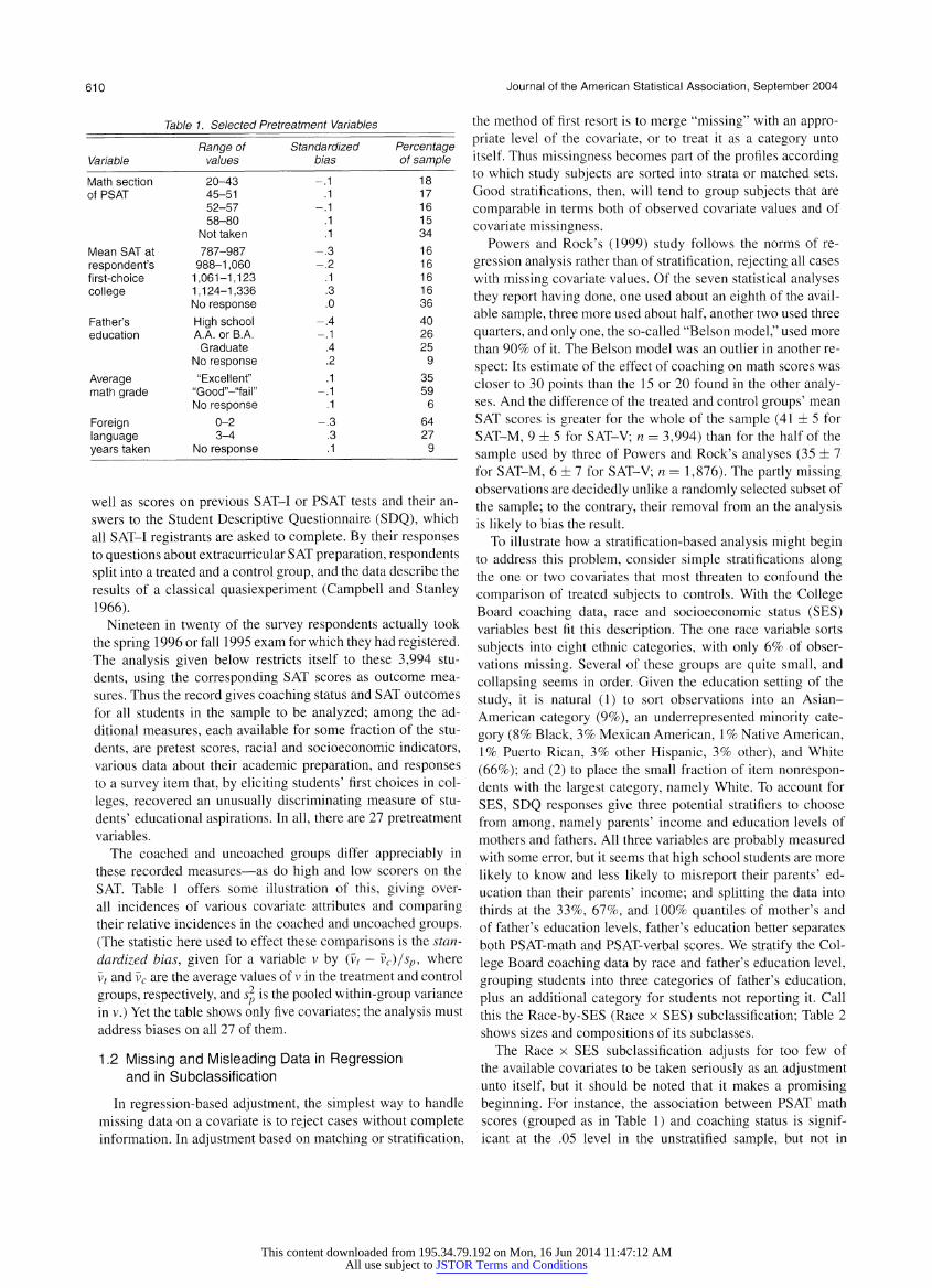
grouping like with like. Figure 1 shows standardized biases for

the unmatched College Board coaching data and for optimal 1:1, 1:3, 1:5, and 1:7 propensity score matchings created

with it.

Observe that the boxplots at the far left and far right of the

figure are identical. This is no accident: The matched sets de

scribed by the rightmost boxplot exclude no controls and, in the

computation of standardized biases, give all controls the same

weight; the same occurs when covariate biases are calculated

for the unmatched sample. In general, if controls are K times as numerous as treated subjects, then adjustment using al:f

matching amounts to no adjustment at all.

The pattern in Figure 1 appears in a number of contexts. It

has led authors such as Dehejia and Wahba (1999) and Smith

(1997) to conclude that whatever its advantages for variance,

attempting to use most or all of the control reservoir invites

sharp penalties in terms of bias. Full matching will turn out to

involve a very different variance-bias tradeoff, however, making

attractive another explanation of the penalties for increased use

of controls seen in Figure 1 : They reflect limitations inherent to

fixed-ratio matching.




in o

o d

Figure 1. Covariate Imbalances in 1:k Matching. Each boxplot rep resents standardized biases in the 99 categories of the 27 categorical covariates along with standardized bias in the propensity score (which in each plot is the uppermost outlier). Strictly speaking, the matching

represented at far right is not a 1:7 matching but a blend of six 1:6 and

494 1: 7 matched sets.

2.3 Full Matching: An Illustration

Full matching subdivides a sample into a collection of

matched sets consisting either of a treated subject and any pos itive number of controls or a control subject and any positive

number of treated persons. These matchings stand in contrast

to the 1 : k matchings considered in the previous section. For

example, one can readily verify that the optimum placement of

the four women and five men in Table 3 into matched sets of one woman and one or two men matches A to V and W, B to X, C to Y, and D to Z, with total cost 3.8. The optimal full match,

depicted in Table 4, reduces this sum to 3.6. Coincidentally, it avoids matching any woman to a man whose grant funding differs from hers by more than a factor of 10?a requirement that, with the help of full matching, could be insisted upon in

the actual study on which the example is based. In the example

problem, neither pair matching nor matching with one or two

controls could have met such a requirement.

Rosenbaum (1991) introduced full matching, Gu and

Rosenbaum (1993) did a simulation study of it, and Marcus

(2000) made use of it to assess the Head Start compensatory education program.

Table 4. Full-Matching Solution to the Matching Problem Posed by Table 3

Women Men

Matched Matched

Subject log10(grant) set Subject log10(grant) set

A B C D

5.7

4.0

3.4

3.1

V

W

X

Y

Z

5.5

5.3

4.9

4.9

3.9

2.4 Matching to Use Every Control

To judge from Figure 1, no way of matching coached to un

coached students at once balances all measured covariates and

places each available control in some matched set. However,

each matching in Figure 1 joins treated and control subjects in

only a single, fixed ratio; full matching may introduce new pos sibilities. This section studies the optimal, in the sense of mini

mizing propensity score distances, full matching of the College Board sample. By its construction, such a matching cannot fail to use every available control, but its success or failure at im

posing balance upon measured covariates remains to be seen.

For each pair i e T and y e C, let a discrepancy 8?j e [0, oo] be given: Small values of 8 indicate desirable matches; large finite ?'s, matches to be avoided; infinite <5's, matches that are

forbidden. A full matching is a partition of all or part of the sam

ple into one-one, one-many, and many-one matched sets, none

of which includes forbidden pairings. Formally, by "full match

ing" let us understand a mapping S of T U C into {0,..., S}, S a positive integer, such that each matched set M = S"1 [s] (1 < s < S) satisfies min(#(M 0 T), #(M 0 C)) = 1, and for ail leMflT and j e M n C, 8 y < oo. The size of a full matching

S is the ordered pair (#(S_1[{1,.. .,5}] nT),#(S)_1[{l,..., S}] n C), indicating the number of treated and the number of control units that S places into matched sets. These definitions are substantially equivalent to those of Rosenbaum (1991).

Given a full-matching problem (C, T, {<$(/}), a full match S of size (c, t) that solves it is optimal among size (c, t)full matches if it minimizes net discrepancy,

E E ?* o) i l\S(i)>0y C,S(i)=S(y)

among all size (c, t) full matches S for (C, T, {<$*/}). An opti mal full match is a minimizer of net discrepancy among size

(#(C), #(T)) full matches, that is, full matches that discard no

units.

In the present analysis, discrepancies 8y are based on the

propensity score: For / e T, j C,

oo, ij belong to different Race x SES subclasses

llogit^iX^-logit^X,))!, otherwise,

where X is the vector of covariates and e(X?), ?(Xj) are fitted

propensity scores. The infinite distances force exact matching on race and father's education. An algorithm to find optimal full matches is described in the Appendix.

Full matching was very successful in removing bias due to

observed covariates. The average within-stratum discrepancy

between treateds and controls, understood as distance along the fitted score, is .05, and the optimal full match removes 99% of the bias in the fitted score. By contrast, average propensity dis tances in the optimal 1:1,1:3, and 1:5 fixed-ratio matchings

were .04, .31, and .69, respectively, with propensity score bias

reductions of 97%, 74%, and 42%. When the sample is parti tioned according to the optimal full match, no covariate exhibits even a hint of association with treatment status; the Cochran

Mantel-Haenszel x2 statistics (see Sec. 1.2) are both nonsignif icant and uniformly close to 0. Evidently, full matching permits use of the control reservoir in its entirety, with no discernible

penalty in terms of bias.

&v=\




fi-I

s -

o _

o 'S T

Jllilfc?uL-il.^,

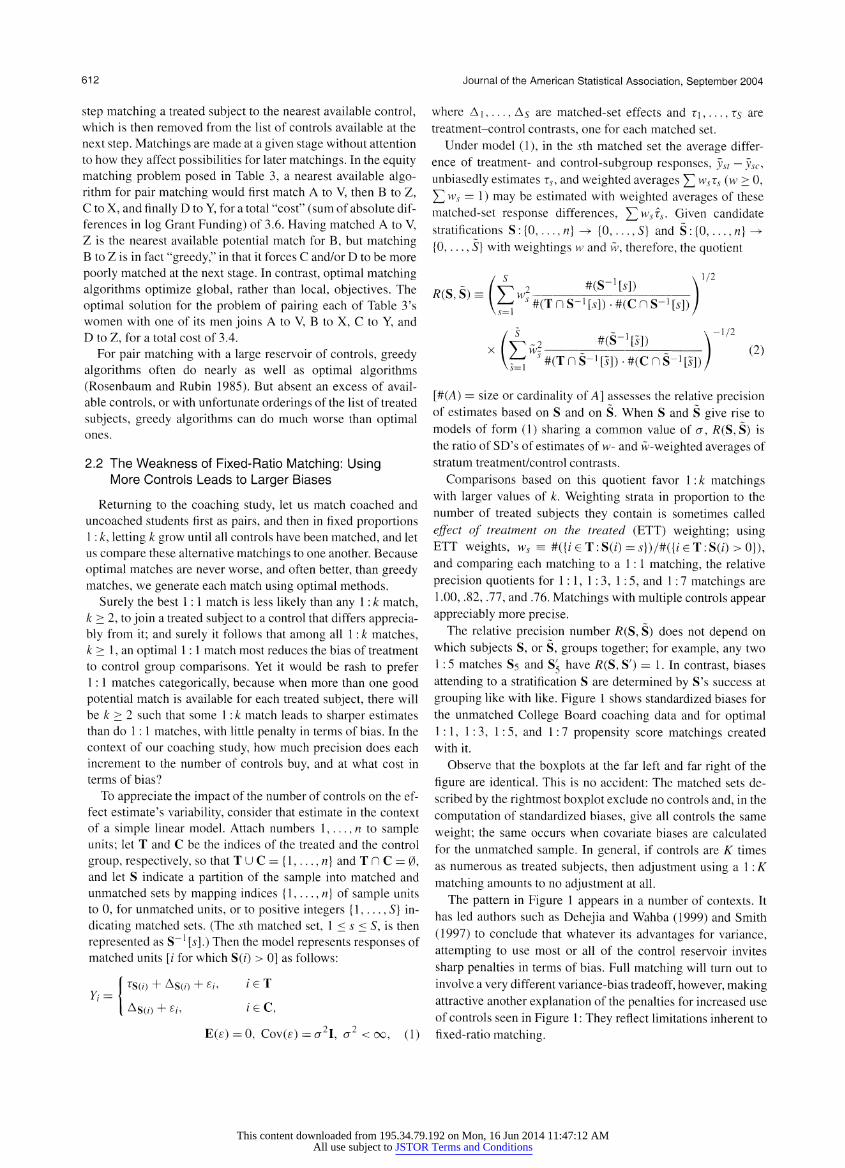
Figure 2. Superimposed Barplots Representing Stratum Sizes of the

Optimal Full Match (gray bars, in background; 466 strata) and the Opti mal [.5, 2] Full Match (in foreground; 491 strata). The contrast between

the two illustrates that in full matching restrictions on treated-to-control

ratios greatly reduce the number of matched sets that are unusually

heavy with control or treated subjects. Vertically aligned bars represent a single matched set, with bar heights above the x axis giving the num

ber of controls in it and bar depth below the x axis showing its share of

treated subjects.

Variance is another issue. Relative to the optimal 1:1 match (Si), the relative precision of the optimal full match is a disappointing .93. This may be better than the optimal

pair match, but it is worse than every one-many match con

sidered in Section 2.2. For instance, the optimal 1:3 matching S3?which substantially reduced covariate imbalances?had

R(S\, S3) = .82. A use of full matching that contains variance as well as bias is described in the next section.

The optimal full match looks strikingly different from any fixed-ratio matching. Most notably, it contains some out

landishly large matched sets: as many as six treated subjects to a control; as many as 161 controls to a treated. Figure 2

represents the composition of its matched sets with stacked

barplots. The black bars in the foreground of Figure 2 repre sent a matching that will be introduced in Section 3.2, but the

gray bars in the background describe the optimal full matching. Adjoining upper and lower bars give the numbers of uncoached

and of coached students in a single matched set, with matched sets arranged from left to right in order of increasing propen

sity score. This arrangement illustrates the natural tendency for

subjects with high scores to be placed in many-one matched

sets, while low propensity score subjects wind up in one-many substrata that are heavy with controls.

3. FULL MATCHING WITH RESTRICTIONS

The optimal full match uses all controls and balances every covariate, but some of its matched sets are too heavy with con

trols, and in others controls are quite sparse. The disparities stand behind the optimal full match's disappointing relative pre cision. And by altering so drastically the weighting of subjects

implicit in the Race x SES subclassification, it engenders esti mates of coaching effects that depend quite strongly on a partic ular propensity score specification. This section produces a full

matching that is similar to the matching of Section 2.4 in that it

balances available covariates without rejecting any controls. In terms of maintaining balance in the relative numbers of treated and control subjects in any matched set, on the other hand, it

does a good deal better than that matching; this improvement increases precision, in the sense that it reduces standard errors

of estimates of treatment effects. Some technical preliminaries are necessary, and it is best to begin with an illustration.

3.1 Full Matching With Restricted Treated-to-Control Ratios

Let us return for the moment to the matching problem of Ta ble 3. As compared to the optimal pair matching, or to the opti mal matching with one or two controls, the optimal full match

given in Table 4 supports assessments of gender equity that have

smaller bias, because it matches men and women more closely in terms of the one covariate being adjusted for. In terms of

variance, however, it is actually worse than those matchings.

Comparing to pair matching and using ETT weights for each

comparison, the precision of a matching into three pairs and a

1:2 set is .97, while a 1:4, 3:1 full matching (as in Table 4) has precision 1.27. One remedy for this is to constrain the re

sult of one's full matching so that the ratios of the numbers of treated and of control subjects in each matched set are either

homogeneous, as in the optimal pair matching, or at least rel

atively homogeneous, as they were in the one-to-two controls

solution to the matching problem of Table 3.

Suppose, for concreteness, that we seek a full matching such that in each matched set, the number of treated subjects divided

by the number of controls ranges from about half up to about

twice what that ratio is in the sample as a whole. For the gender

equity matching problem, the overall ratio of treated (women) to control subjects (men) is 4:5, so we would seek individual

matched sets with treated-to-control ratios of about 1:2.5 up to

1.6:1. Matched sets with 2.5 controls or 1.6 treated subjects are

of course impossible, so we require a rounding convention. Let

us be permissive rather than strict, interpreting the present re

quirement so as to permit matched sets with treated-to-control

ratios of 1:3 up to 2:1. (By establishing the conventions in this way, we reduce the potential for inadvertently imposing a

restriction that makes matching infeasible, as would occur in

the equity matching problem if a restricting factor of .75, rather than 1/2, were placed on the reduction in the ratio of treated

subjects to controls, and if the resulting upper limit of 1.67 con

trols per treated subject were to be interpreted strictly.) The full matching that minimizes costs while adhering, un

der this interpretation, to the half-to-twice restriction on the ra

tio of women to men is as follows: woman A is matched to men V and W, and B to X and Y; while women C and D are both

matched to Z. The restrictions lead to a somewhat greater total

cost, 3.7 versus 3.6. Even with restrictions, however, full match

ing again makes it possible to avoid matching men and women

whose log I0 (Grant Funding) differs by more than 3. At a small

price, then, one secures a substantial improvement in precision:

Writing Sr for the optimal full matching with constraints and

S/ for Table 4's unconstrained optimal full matching, one has

?(Sr,S/) = .82.

Let us place these ideas into a suitable formalism. A match

ing S subdivides U if for all subject indices / and j, S(0 =




SO') entails U(z') = UO"). When S subdivides U, for each

matched set M of S there is a stratum U of U, that is, U ?

U~l[s] for some s > 1, such that M ? U. Given a stratifi

cation U, call the ratio of treated subjects to controls in U

the U-treatment odds for stratum U. When S subdivides U, a matched set M of S has both S-treatment odds, ds(M), and U-treatment odds, ?/U(M), namely the U-treatment odds

for the stratum U of U that contains it. In the gender eq

uity example, the null stratification Uo : {A, B, C, D, V, W, X,

Y, Z} t-> {1} is subdivided by Sr. Regarding women as treated

and men as control subjects, the Uo-treatment odds for Uo's

lone stratum, duo({A, B, C, D, V, W, X, Y, Z}), are 4:5, as are

the Uo-treatment odds in each of Sr's matched sets; but Sr's three matched sets have Sr-treatment odds of dSr ({A, V, W}) =

1:2, dSr({B, X, Y}) = 1 :2, and ds> ({C, D, Z}) = 2:1.

A matching S that subdivides U respects a thickening cap of u, u > 1, if the S- and U-treatment odds obey the relation

\udv(M)]:\, udv(M)> 1

1: |_(m?/u(M))_1J, udv(M) < 1

for each matched set M of S. Such an S nowhere increases the

ratio of treated to control subjects to more than roughly u 100%

of what it would have been under U. As a subdivision of the

null stratification Uo, the restricted full matching Sr respects a

thickening cap of 2.

Similarly, the subdivision of U into S conforms to a thinning

cap of / if 0 < / < 1 and for each matched set M of S,

?S(M)<{ ",,? _!, ? (4)

|_Zdu(M)J:l, ldv(M) > 1

l:\(ldv(M))~l], /?/U(M)< 1. ds(M)>\

- _ ^ _H ^ (5)

As a subdivision of Uo, Sr holds to a thinning cap of 1 /2. An [/, u\-subdivision ofU is a subdivision of U respecting a

thinning cap of / and a thickening cap of u. An optimal [/, u\ subdivision ofU is an [/, u]-subdivision of U with minimal net

discrepancy [cf. (3)] among full matches that subdivide U and

conform to thinning and thickening caps of / and u. Sr is an

optimal [.5, 2]-subdivision of Uo

3.2 Restricted Full Matching for the

Board Sample

Now let U denote the Race x SES subclassification (Sec. 1.2). We seek an optimal [/, ̂ -subdivision of U, / < 1 and u > 1,

that adequately balances each covariate while keeping / and u

as close to one as is consistent with this aim.

One-half and two are a natural pair of caps with which to

start: Alter the treatment odds within strata, they say, by no

more than a factor of 2. Against the optimal [.5,2] full match,

testing each of the 27 covariates separately using statistics of

the Mantel-Haenszel (MH) type (cf. Sec. 1.2) yields no results

of significance at the nominal .05 level; only with the parents' income variable is there a hint of association (M2/df

= 8.9/4,

p = .06). Alternatively, the battery of tests may be directed

at subjects without missing covariate data. The 27 additional

MH tests that exclude those matched sets containing a subject

missing data on the relevant covariate also fail, for the most

part, to reject null hypotheses of no association. The excep

tions are a test giving some thin evidence of association be

tween the parents' income variable and treatment status, with

Propensity score

m ^ o

Demographic profile X

o o

o <* , *b

College preferences

J--*o

Experience with the test

% No. of courses in high school, by subject

o

High school grades

PSAT verbal PSAT math Prior SAT verbal Prior SAT math

Gender First language Ethnicity Parent's income Mother's education Father's education

Public vs. private Avg. SAT at 1st choice college

Importance Nervousness Self-assessment

English Foreign Language Math Natural Science Social science

G PA English Math Natural Science Social Science

I-1-1-1 -0.5 -0.3 -0.1 0.1

Standardized Biases

?1-1-1-T" 0.3 0.5 0.7 0.9 1.1

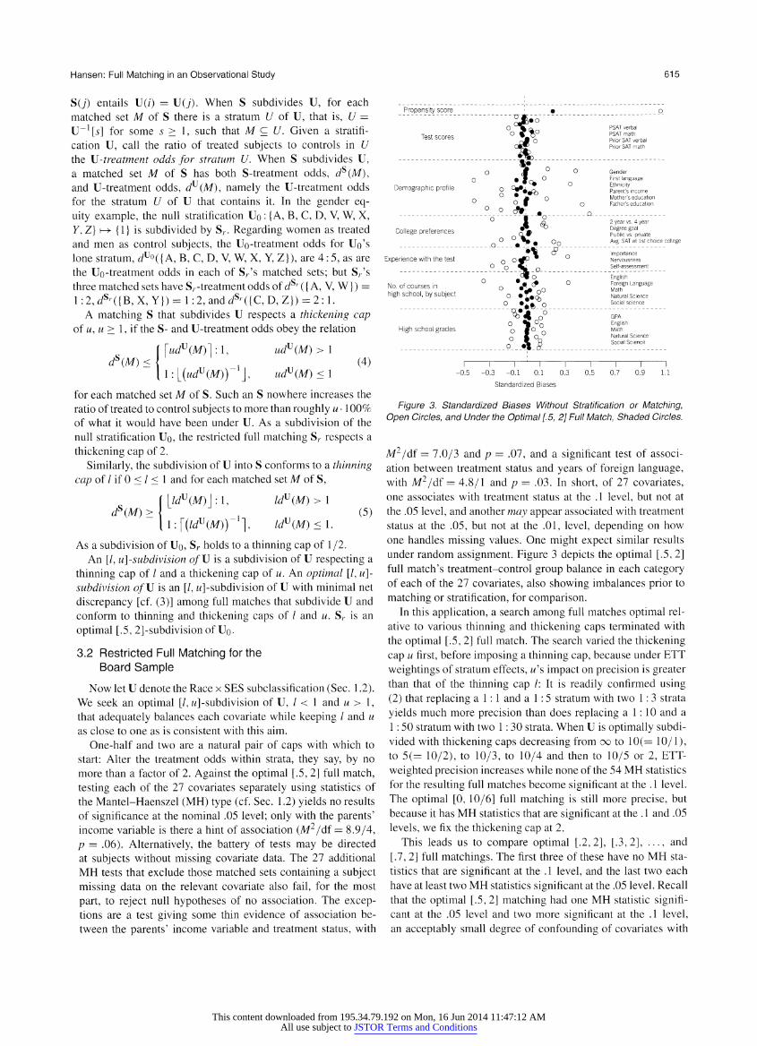
Figure 3. Standardized Biases Without Stratification or Matching,

Open Circles, and Under the Optimal [.5, 2] Full Match, Shaded Circles.

M2/df =

7.0/3 and p ? .07, and a significant test of associ

ation between treatment status and years of foreign language,

with M2/df = 4.8/1 and p = .03. In short, of 27 covariates,

one associates with treatment status at the . 1 level, but not at

the .05 level, and another may appear associated with treatment

status at the .05, but not at the .01, level, depending on how

one handles missing values. One might expect similar results

under random assignment. Figure 3 depicts the optimal [.5, 2] full match's treatment-control group balance in each category

of each of the 27 covariates, also showing imbalances prior to

matching or stratification, for comparison.

In this application, a search among full matches optimal rel

ative to various thinning and thickening caps terminated with

the optimal [.5, 2] full match. The search varied the thickening

cap u first, before imposing a thinning cap, because under ETT

weightings of stratum effects, w's impact on precision is greater

than that of the thinning cap /: It is readily confirmed using

(2) that replacing a 1:1 and a 1:5 stratum with two 1: 3 strata

yields much more precision than does replacing a 1: 10 and a

1: 50 stratum with two 1: 30 strata. When U is optimally subdi

vided with thickening caps decreasing from oo to 10(= 10/1), to 5(= 10/2), to 10/3, to 10/4 and then to 10/5 or 2, ETT

weighted precision increases while none of the 54 MH statistics

for the resulting full matches become significant at the . 1 level.

The optimal [0, 10/6] full matching is still more precise, but

because it has MH statistics that are significant at the . 1 and .05

levels, we fix the thickening cap at 2.

This leads us to compare optimal [.2,2], [.3,2], ..., and

[.7, 2] full matchings. The first three of these have no MH sta

tistics that are significant at the .1 level, and the last two each

have at least two MH statistics significant at the .05 level. Recall

that the optimal [.5,2] matching had one MH statistic signifi cant at the .05 level and two more significant at the . 1 level, an acceptably small degree of confounding of covariates with




CL

un

matched [0,2.5] [0,2] [0,1.7] [.4,2] [.5,2] [.6,2]

Figure 4. Standardized Biases and Relative Precision [R(-, uncon

strained full match)] of Optimal Stratifications With Variously Con

strained Match Ratios.

treatment status. These comparisons lead us to prefer a thinning

cap of .5. (Had we selected first a thinning and then a thicken

ing cap rather than the reverse, this procedure would have led us instead to the optimal [.6, 2.5] full match.) Figure 4 displays standardized biases and relative precisions /?(*, U), where U is

the optimal 1:1 match, for optimal [/, u] full matchings with

various / and u.

3.3 Reduced Sensitivity to Model Specification

The model here used to estimate propensity scores lacks in

teraction terms among its independent variables and involves no auxiliary modeling of data missingness. This puts it among the simplest of models one might use for propensity score es

timation; it was chosen for this reason. Certainly, more elab

orate propensity score models have been used; Rosenbaum

and Rubin (1984), for example, employed a stepwise variable

selection procedure to select main effects and then interaction

terms, and D'Agostino and Rubin (2000) modeled item miss

ingness explicitly, fitting their model using the EM algorithm. The matching strategy taken here, stratifying on variables

strongly predictive of treatment status before full matching with

restrictions, aimed to limit the dependence of the analysis on

any one specification of the treatment assignment model. To as

sess its success at this, a more saturated propensity score model

was fit. As right-hand-side variables, this model has eight in

teractions and 17 main effects of the original variables, cho sen by backward-forward stepwise variable selection. Using this model's fitted propensity score, evaluations of thickening and then thinning caps lead one to prefer an optimal [.4,2] full

match. Call this new matching S2, and the matching selected in

Section 3.2, Si. Both full matches use all of 3,494 controls, and in most cases

the two matchings place these control subjects into matched sets

of very similar sizes: 20% of the 3,494 go into matched sets of

precisely the same size; for 72% of controls j, the S2-treatment odds of /s S2 stratum are no more than 4/3, and no less

than 3/4, of the Si-treatment odds of/s Si stratum. Because a subject's contribution to our effect estimates is determined by

the configuration of the matched set into which it is placed, it

should be no surprise that the two full matchings lead to similar

estimates of the coaching effect.

4. ESTIMATING TREATMENT EFFECTS

To estimate treatment effects, a model such as (1) must be

supplemented with a causal formalism and appropriate causal

assumptions. For this analysis, the most natural setup is that of

Rubin (1977), who posits random variables Yt and Yc both for outcomes under the control condition and for outcomes under

the treatment condition. Adding the assumption that these vari

ables are conditionally independent of the treatment assignment variable (Z) given the covariates (X) makes inference about treatment effects possible.

Using ETT weighting to combine by-stratum treatment

control differences, the [.5, 2] matching leads to aggregate con

trasts of 26 points on the math section and 1 point on the verbal.

Under causal assumptions as presently discussed, these esti mate effects of coaching on the coached. Using model (1), the

accompanying standard errors are 5 and 5 points. By contrast, the unadjusted differences of treated and control group means

were 41 (?5) and 9(?5) points. As one might expect, those matchings that fail to reduce

discernible biases to an indiscernible level give higher effect

estimates. For example, the nearly fixed-ratio matching that re

spects Section 1.2's subclassification while using all controls, that is, the optimal [1,1] subdivision of the Race x SES sub

classification, offers estimates of 30(?5) and 2(?5). Of all

matchings that respect the Race x SES subclassification, this

had the most favorable relative precision quotients; yet its es

timated standard errors are only negligibly smaller than those

of the [.5,2] match, while its poorer balance translates to ap

parent biases of one or more standard errors in estimates of the

coaching effect. Conversely, those matchings that did reduce

observed biases to indiscernibility gave lower estimates. The

optimal [.6, 2.5] full match of Section 3.2 gives estimates of

23(?5) and 0(?5), and Section 3.3's [.4,2] full match leads to

estimates of 23 (?5) and 0(?5).

4.1 Heterogeneity of Coaching Effects

Unlike both pair matching and analysis of covariance, full

matching's estimates and standard errors do not assume treat

ment effects to be the same across units; they average estimates of individual treatment effects that can, in principle, be quite different. This is especially advantageous in a coaching study based on a representative national sample, since coaching pro

grams differ widely in duration, rigor, and approach. As a re

laxation of the constant-effect model, consider the hypotheses of 12 math and 12 verbal effects, one for each Race x SES sub

class. By dint of the exact matching on race and father's edu

cation level, the matched-set coaching effects are nested within subclass coaching effects, and the three models?the constant

effect model, the 12-effects model, and model (1), with its

494 separate treatment effects?can be compared by an analy

sis of variance (ANOVA). In either the math or the verbal case, F tests based on the ANOVA reject the constant-effect model in favor of either the 12-effects model or model (1), and the

12-effects model cannot be rejected from within (1). The hy

pothesis that there is a single, constant treatment effect is un

tenable. Granted, given the variety among interventions here




grouped together as "treatments," there is little to recommend

such hypothesis; yet previous coaching studies have often been

analyzed using regression models that are built upon it.

4.2 Very Large and Very Small Coaching Effects:

Which Are More Plausible?

Is it strange that structured, extended training for the SAT

should produce, on the average, no more than a negligible ben

efit in verbal scores? In interpreting this result, one should bear

in mind that the control condition is not the absence of prepa ration for the SAT. In this observational study, "not coached"

means only "did not participate in a program of preparation for

the SAT-I that was held outside of school." Controls may have, and by and large did, practice and otherwise prepare for the tests

on their own or in school (Powers and Rock 1999); it is possible that these preparations were sometimes more effective than for

mal coaching. Indeed, our matching also facilitates estimating what effect the treatment would have had on the controls, were

they treated, and the results of this calculation suggest that some

controls benefited by selecting alternative test preparations: The

effect of treatment for the controls is estimated at 3 ? 7 points on the math section and ? 8 ? 7 points on the verbal. Evidently, whether and to what degree coaching is beneficial varies greatly from student to student.

Our analysis's allowance for heterogeneous coaching ef

fects permits it to speak more directly to the coaching com

panies' claims than did Powers and Rock's analyses. Recall

that the Princeton Review claims its students' average benefit

is 140 points in the combined score (Princeton Review 2004), and that Kaplan Educational Centers have said that students

benefit from their courses, on average, by 120 points (Zehr

2001). Further, a Kaplan spokesman has argued that very dif

ferent gains are to be expected from Kaplan's programs as op

posed to those of many of its competitors; shorter, cheaper, and

untested programs abound, and smaller benefits are to be ex

pected from them (Kolata 2001). The multiple-regression type of analysis favored by Powers and Rock cannot speak directly to this argument, as they assume uniform treatment effects, but

the matching-based analysis of this article can.

At least 41% of coached students in the College Board sam

ple had been coached by either Kaplan Educational Centers or

the Princeton Review. Consider the hypothesis that Kaplan and

the Princeton Review offer varying coaching benefits that aver

age to 120 points, say. To permit a robust test of this hypothesis, let us supplement it with the unlikely assumption that all other

companies ' coaching benefits average to 0. Even with models

of form (1), which grant each matched set its own treatment

effect, the upper 95% confidence bounds for the math and ver

bal effects (of coaching upon the coached) are about 37 and 11

points. Combined, these fall short of the 49-point overall av

erage effect that Kaplan's and the Princeton Review's claims

would, at a minimum, entail. The hypothesis is rejected.

5. DISCUSSION: UPDATING THE LIMITATIONS OF MATCHING

Observational studies compare persons who received a spec

ified treatment to others who did not, adjusting for pretreatment differences between treated and comparison groups. Broadly,

these adjustments are effected either by regression modeling or

by stratification. Regression adjustments assume that we know

or can reliably discern patterns relating pretreatment, treatment,

and response variables, and require the statistician to spec

ify and fit a corresponding statistical model. Adjustment by stratification assumes only that treatment and control groups

sufficiently alike in terms of pretreatment characteristics are

comparable in terms of response to treatment; but it requires the statistician to make precise what it means for groups to be

sufficiently alike prior to treatment, and it requires a method for

grouping subjects into sufficiently uniform blocks.

Matching and stratification are old and trusted methods of

adjustment for observational studies, but the difficulty of im

plementing them led earlier practitioners to prefer regression. Cochran (1972) warned that in "larger studies... matching be comes impractical." In smaller and more manageable settings,

Cochran recommended stratification as adjustment only for the one or two most important variables. Adjusting by matching or stratification for more than a few variables seemed hope

less: In one widely cited case, Chapin (1947) started with

671 treated subjects and 523 controls but found only 23 treated

control pairs matching exactly on six categorical covariates.

Citing these concerns, Cochran concluded: "[I]f there are say Ax variables... [then our] recourse is to model construction and

analysis based on the model."

Cochran gave this pessimistic assessment some 30 years ago.

Advances since then have made observational data no more

amenable to exact matching than they ever were, but the intro

duction of propensity scores (Rosenbaum and Rubin 1984) has

greatly facilitated approximate matching on many variables; re

sults possible with propensity scores and optimal full matching stand in striking contrast with Cochran's. In analytic studies,

Cochran (1965) studied stratification on a single variable for

treatment and control groups no more than a standard deviation

apart. The schemes he studied removed as little as 57% and no

more than 89% of the bias along the covariate. In the present case study, optimal full matching removes as much as 99% of

the bias along a propensity score on which the treated and con

trol means are separated by 1.1 SD's. In so doing, we have seen,

it reduced to insignificance biases along 27 covariates, and it

made use of more, not less, of the data than did regression

based analyses. With flexible matching routines increasingly available, will regression adjustment for observational studies soon be obsolete?

APPENDIX: OLSEN'S ALGORITHM: A UNIFIED APPROACH TO OPTIMAL MATCHING

This appendix presents the algorithm used in this article to cre

ate optimal matchings. We employ a variant of the approach of

Rosenbaum (1991), who presented (sec. 7) a general method for trans

lating full-matching problems into network flow problems, which can

in turn be solved efficiently using any of several widely available al

gorithms. According to Section 2.4, full-matching problems may be

associated with triples (T, C, {<5//}). A full-matching problem is fea

sible if it has a solution with finite total discrepancy. An optimal so

lution is one in which the average discrepancy within matched sets,

Es E/eTjeC : S^S?)^///^ W.fi e T x C : S(i) = SO') = s}), is as small as it would be under any other solution. Rosenbaum (1991 )

represented such a problem as a graph with a node for every treated and

every control, plus a node called "Source" and another called "Drain,"




with edges from Source to each treated node, from / toj when 5/y < co,

and from every control node j to Drain. A network flow problem is as

sociated with this graph in such a way that optimal flows through the

network correspond to optimal full matchings.

By constrained full-matching problem, let us understand a full

matching problem (T; C; {<$//}) accompanied by upper and lower lim

its (L, U) on the number of controls per treated and upper and lower

limits (?, U) on the number of treateds per control; a constrained prob lem (T; C; {8ij}; L, U, ?, ?) is feasible if there exists a solution of the

problem (T; C; {<%}) which respects the constraints. The problem of

finding an optimal [/, w]-subdivision of a stratification U, if one ex

ists, is easily translated to a sequence of constrained full-matching

problems?one for each stratum of U. In the applications discussed

previously, controls outnumber treated subjects in each stratum, with

the consequence that L < 1 for each constrained full matching problem that had to be solved.

To handle constrained full-matching problems with L = \ or 0,

Olsen (1997, chap. 6) modified Rosenbaurrfs (1991) algorithm in sev

eral important ways. First, in addition to Source and Drain nodes and a

node for each study subject, there is an additional node, labeled "Over

flow," with edges connecting it to each treated and to each control

node; there is no cost for sending units of flow along these edges.

Second, a negligible amount e > 0 is added to each discrepancy 8y. In Olsen's network flow problem, the upper and lower capacity limits

for edges of various types are as follows: for edges from treateds to

controls, [0, 1]; for an edge from Source to a treated, say /, [0, U]\ for

an edge from a treated, i, to Overflow, [0, U ? L]; for an edge from a

control,y", to Overflow, [0, U ? 1]; and for an edge from a control,y, to

Drain, [0, 1]. The supply (exogenous inflow) is 0 at each node except

Source, Drain, and Overflow, at which supplies are U #T, ?p #C,

and p #C ?

U #T, respectively. Here, p is the proportion of avail

able controls that are to be matched to treated subjects; thus p < 1, and

p < 1 only if L = 0. The constrained full-matching problem is feasible

if and only if the Olsen network flow associated with it is feasible. In

this case, an optimal flow through the network corresponds to a full

match that is optimal among appropriately constrained full matches.

To implement Olsen's algorithm, I created functions calling the

RELAX-IV network optimization routine of Bertsekas and Tseng

(1994) from the R environment (r-project.org); this code is bundled

together in an add-on package to R, "optmatch," information about

which can be found on my Web site.

[Received April 2003. Revised January 2004.]

REFERENCES

Agresti, A. (1990), Categorical Data Analysis, New York: Wiley. Bertsekas, D. P., and Tseng, P. (1994), "RELAX-IV: A Faster Version of the

RELAX Code for Solving Minimum Cost Flow Problems,'1 Technical Re

port P-2276, Massachusetts Institute of Technology, available at mit.edu/

dimitrib/www/noc.htm.

Briggs, D. (2001), "The Effect of Admissions Test Preparation: Evidence From

NELS:88," Chance, 14, 10-21.

Campbell, D., and Stanley, J. (1966), Experimental and Quasi-Experimental Designs for Research. Boston: Houghton Mifflin.

Chap?n, F. (1947), Experimental Designs in Sociological Research, New York:

Harper & Row.

Cochran, W. G. (1965), "The Planning of Observational Studies of Human Pop ulations," Journal of the Royal Statistical Society, 128, 234-266.

- (1972), "Observational Studies," in Statistical Papers in Honor of

George Snedecor, Iowa State University Press, pp. 77-90.

D'Agostino, R., Jr., and Rubin, D. (2000), "Estimating and Using Propensity Scores With Partially Missing Data," Journal of the American Statistical As

sociation, 95, 749-759.

Dehejia, R., and Wahba, S. (1999), "Causal Effects in Nonexperimental Studies:

Reevaluating the Evaluation of Training Programs," Journal of the American

Statistical Association, 94, 1053-1062.

Gu, X., and Rosenbaum, P. (1993), "Comparison of Multivariate Matching Methods: Structures, Distances, and Algorithms," Journal of Computational and Graphical Statistics, 2, 405^20.

Kolata, G. (2001), "Admissions Test Courses Help, but Not So Much, Study Finds," The New York Times, 1, 16.

Mantel, N. (1963), "Chi-Square Tests With One Degree of Freedom: Exten

sions of the Mantel-Haenszel Procedure," Journal of the American Statistical

Association, 58, 690-700.

Marcus, S. M. (2000), "Estimating the Long-Term Effects of Head Start," in Into Adulthood: A Study of the Effects of Head Start, eds. S. Oden,

L. J. Schweinhart, and D. P. Weikart, Ypsilanti, MI: High/Scope Press,

Chap. F, pp. 179-200.

Ming, K., and Rosenbaum, P. (2000), "Substantial Gains in Bias Reduc

tion From Matching With a Variable Number of Controls," Biometrics, 56, 118-124.

Olsen, S. (1997), "Multivariate Matching With Non-Normal Covariates in Ob servational Studies," Ph.D. thesis, University of Pennsylvania.

Powers, D., and Rock, D. (1999), "Effects of Coaching on SAT I: Reasoning Test Scores," Journal of Educational Measurement, 36, 93-118.

Princeton Review (2004), "SAT Classroom Courses for Class of 2005," avail able at princetonreview.com.

Rosenbaum, P. (1984), "The Consequences of Adjustment for a Concomitant Variable That Has Been Affected by the Treatment," Journal of the Royal Statistical Society, Ser. A, 147, 656-666.

- (1991), "A Characterization of Optimal Designs for Observational

Studies," Journal of the Royal Statistical Society, 53, 597-610.

Rosenbaum, P., and Rubin, D. (1984), "Reducing Bias in Observational Studies

Using Subclassification on the Propensity Score," Journal of the American

Statistical Association, 79, 516-524. -

(1985), "Constructing a Control Group Using Multivariate Matched

Sampling Methods That Incorporate the Propensity Score," The American

Statistician, 39, 33-38.

Rubin, D. B. (1977), "Assignment to Treatment Group on the Basis of a Co

variate (Corr: V3 P384)," Journal of Educational Statistics, 2, 1-26.

Smith, H. (1997), "Matching With Multiple Controls to Estimate Treatment

Effects in Observational Studies," Sociological Methodology, 27, 325-353.

Zehr, M. (2001), "Study: Test-Preparation Courses Raise Scores Only Slightly," Education Week, available at ed-week.com.



Documents

Full Matching in an Observational Study of Coaching for the SAT