Full distribution function of quantum noise: from interference

experiments to string theory

Full distribution function of quantum noise: from interference

experiments to string theoryVladimir Vladimir GritsevGritsev

Collaboration:

EhudEhud AltmanAltman -- WeizmannWeizmannEugene Eugene DemlerDemler -- HarvardHarvardAdiletAdilet ImambekovImambekov - Harvard YaleHarvard YaleAnatoliAnatoli PolkovnikovPolkovnikov -- Boston Uni.Boston Uni.

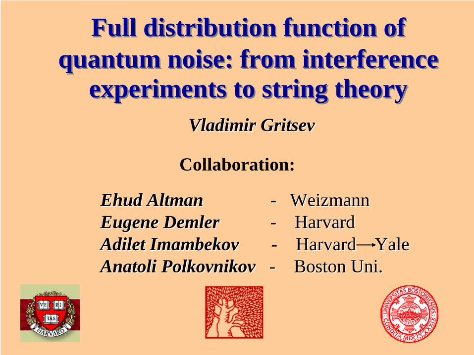
Outline

1. Brief reminder

2. FDF and interference of interacting 1D systems

3. FDF and mapping to statistics of random surfaces

4. FDF and other problems

5. FDF and AdS/CFT correspondenceFDF and Langlands duality

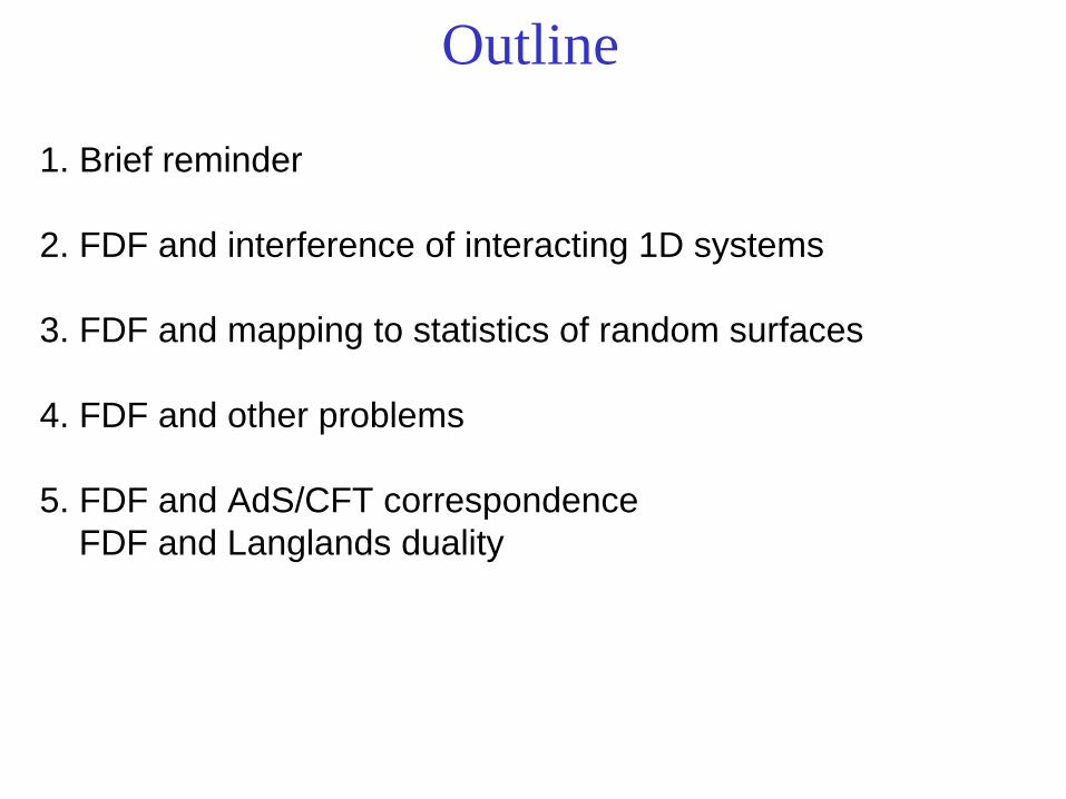
1. Brief reminder (of some notions from talks by

I. Bloch, J. Dalibard, J. Schmiedmayer, A. Polkovnikov)

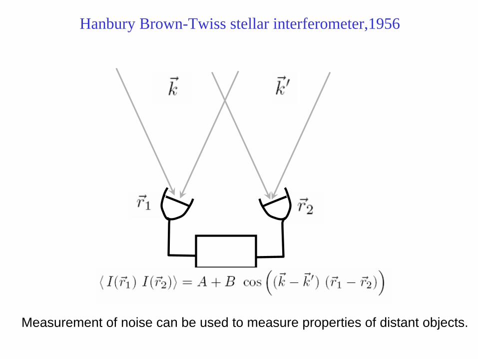
Hanbury Brown-Twiss stellar interferometer,1956

Measurement of noise can be used to measure properties of distant objects.

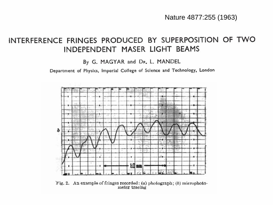
Nature 4877:255 (1963)

x

z

z1

z2

AQ

†int 1 20

( ) exp( ) ( ) ( ) c.c.L

x iQx a z a z dzρ + ⇒∫

2 † †1 1 1 2 2 1 2 2 1 20 0( ) ( ) ( ) ( )

L L

QA a z a z a z a z dz dz∫ ∫

Identical homogeneous condensates:Identical homogeneous condensates:

22 †

1 10( ) (0)

L

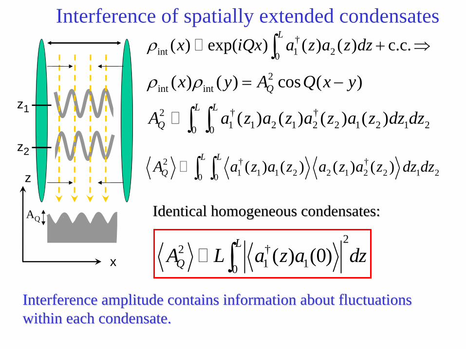
QA L a z a dz∫Interference amplitude contains information about fluctuations Interference amplitude contains information about fluctuations within each condensate.within each condensate.

2int int

2 † †1 1 2 1 2 2 1 2 1 20 0

( ) ( ) cos ( )

( ) ( ) ( ) ( )

Q

L L

Q

x y A Q x y

A a z a z a z a z dz dz

ρ ρ = −

∫ ∫

Interference of spatially extended condensates

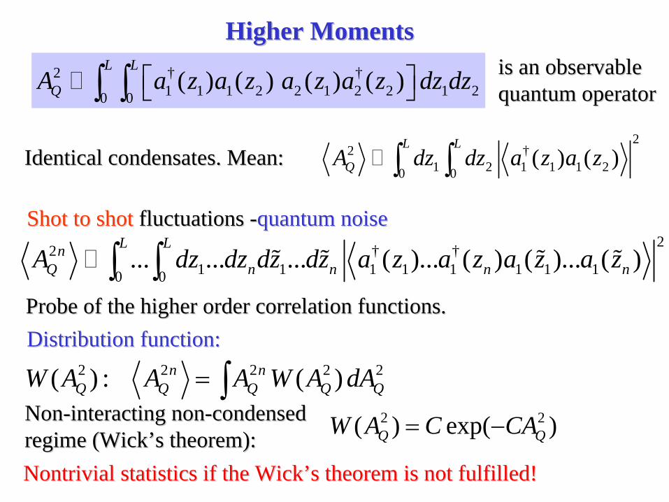
Higher MomentsHigher Moments2 † †

1 1 1 2 2 1 2 2 1 20 0( ) ( ) ( ) ( )

L L

QA a z a z a z a z dz dz⎡ ⎤⎣ ⎦∫ ∫ is an observable is an observable quantum operatorquantum operator

22 †

1 2 1 1 1 20 0( ) ( )

L L

QA dz dz a z a z∫ ∫Identical condensates. Mean:Identical condensates. Mean:

Shot to shotShot to shot fluctuations fluctuations --quantum noisequantum noise22 † †

1 1 1 1 1 1 1 10 0... ... ... ( )... ( ) ( )... ( )

L LnQ n n n nA dz dz dz dz a z a z a z a z∫ ∫ % % % %

Probe of the higher order correlation functions. Probe of the higher order correlation functions.

Nontrivial statistics if the Wick’s theorem is not fulfilled!Nontrivial statistics if the Wick’s theorem is not fulfilled!

Distribution function:Distribution function:2 2 2 2 2( ) : ( )n nQ Q Q Q QW A A A W A dA= ∫

NonNon--interacting noninteracting non--condensed condensed regime (Wick’s theorem):regime (Wick’s theorem):

2 2( ) exp( )Q QW A C CA= −

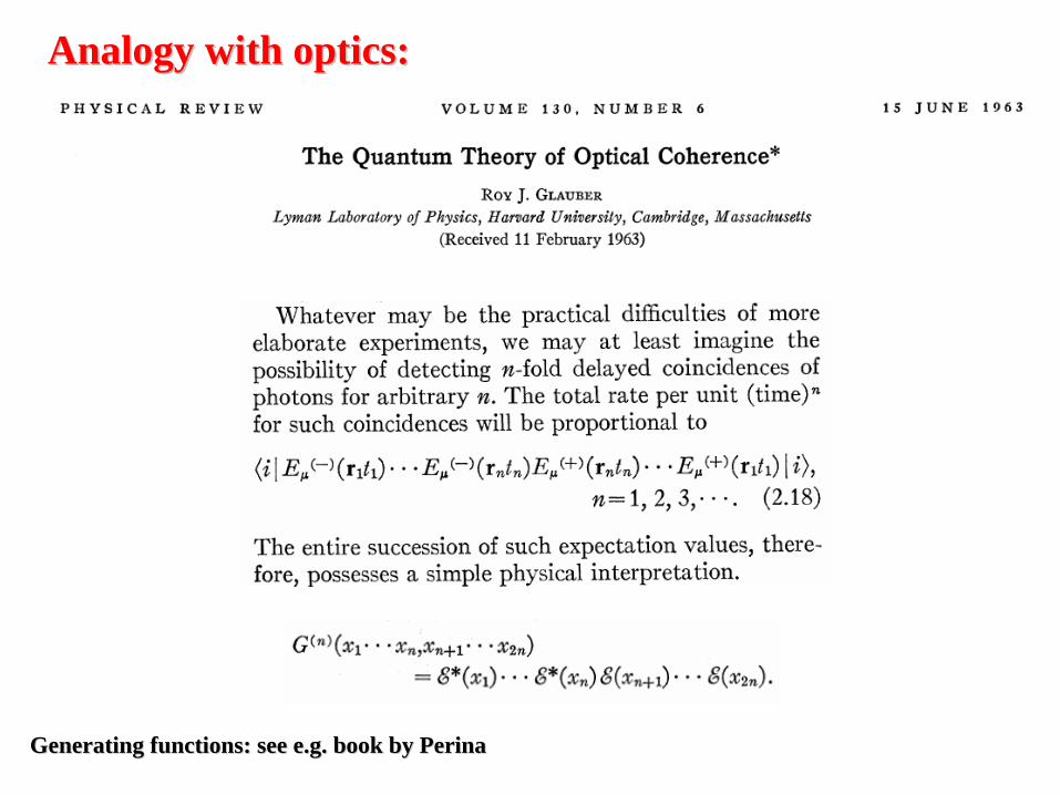
Analogy with optics:Analogy with optics:

Generating functions: see e.g. book by Generating functions: see e.g. book by PerinaPerina

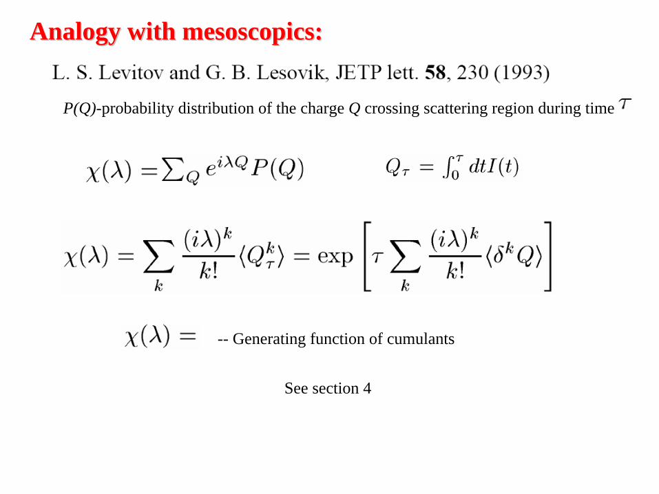
P(Q)-probability distribution of the charge Q crossing scattering region during time

Analogy with Analogy with mesoscopicsmesoscopics::

-- Generating function of cumulants

See section 4

2. FDF and interference of interacting 1D systems

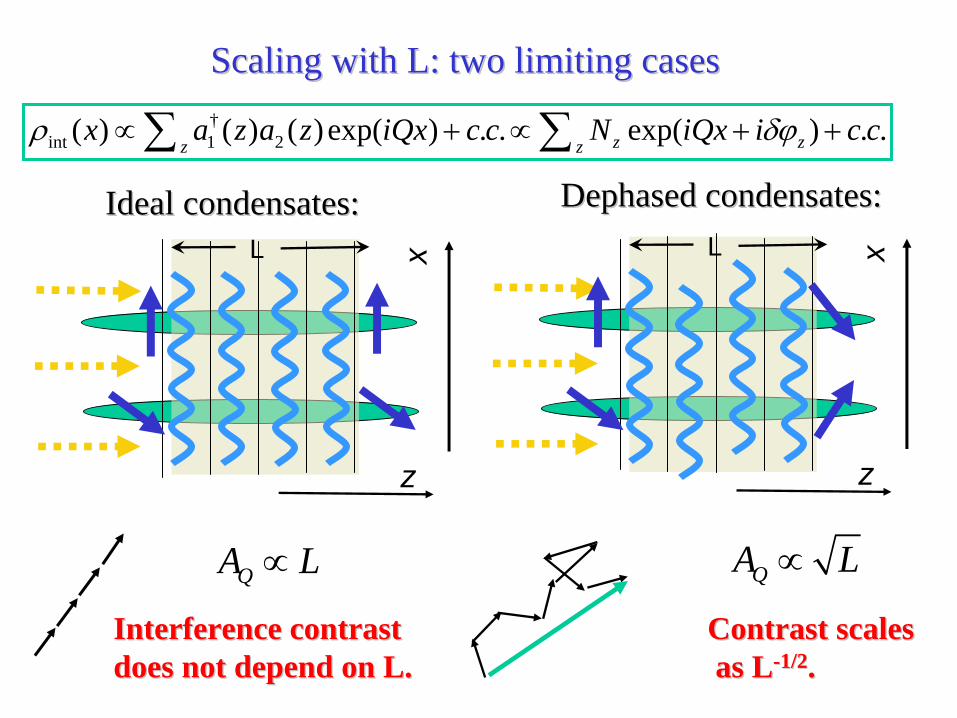
Scaling with L: two limiting casesScaling with L: two limiting cases†

int 1 2( ) ( ) ( ) exp( ) . . exp( ) . .z zz zx a z a z iQx c c N iQx i c cρ δϕ∝ + ∝ + +∑ ∑

QA L∝

Ideal condensates:Ideal condensates:L x

z

Interference contrast Interference contrast does not depend on L.does not depend on L.

L x

z

DephasedDephased condensates:condensates:

QA L∝

Contrast scalesContrast scales as Las L--1/21/2..

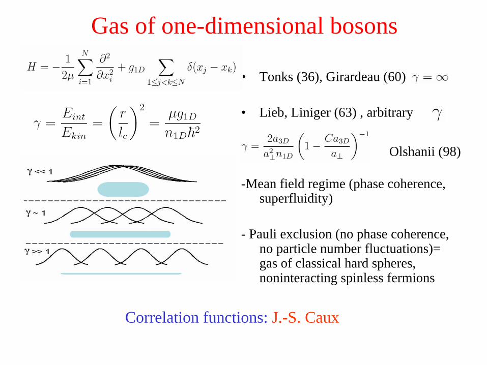
Gas of one-dimensional bosons

• Tonks (36), Girardeau (60)

• Lieb, Liniger (63) , arbitrary

-Mean field regime (phase coherence, superfluidity)

- Pauli exclusion (no phase coherence, no particle number fluctuations)= gas of classical hard spheres, noninteracting spinless fermions

Correlation functions: J.-S. Caux

Olshanii (98)

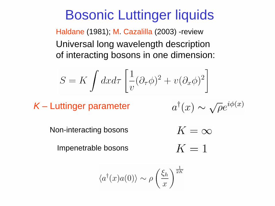
Bosonic Luttinger liquids

Universal long wavelength description of interacting bosons in one dimension:

K – Luttinger parameter

Non-interacting bosons

Impenetrable bosons

Haldane (1981); M. Cazalilla (2003) -review

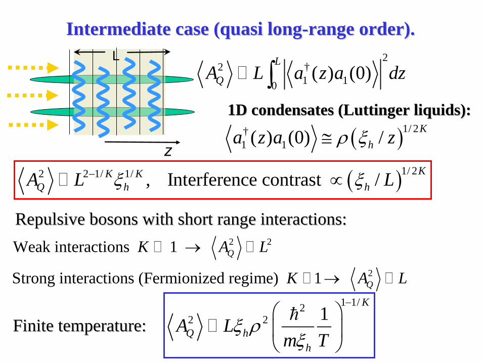
Intermediate case (quasi longIntermediate case (quasi long--range order).range order).2

2 †1 10( ) (0)

L

QA L a z a dz∫

z

1D condensates (1D condensates (LuttingerLuttinger liquids):liquids):

( )1/ 2†1 1( ) (0) / K

ha z a zρ ξ≅

L

( )1/ 22 2 1/ 1/ , Interference contrast / KK KQ h hA L Lξ ξ− ∝

Repulsive bosons with short range interactions: Repulsive bosons with short range interactions: 2 2

2

Weak interactions 1

Strong interactions (Fermionized regime) 1

Q

Q

K A L

K A L

→

→

Finite temperature:Finite temperature:1 1/2

2 2 1K

Q hh

A Lm T

ξ ρξ

−⎛ ⎞⎜ ⎟⎝ ⎠

h

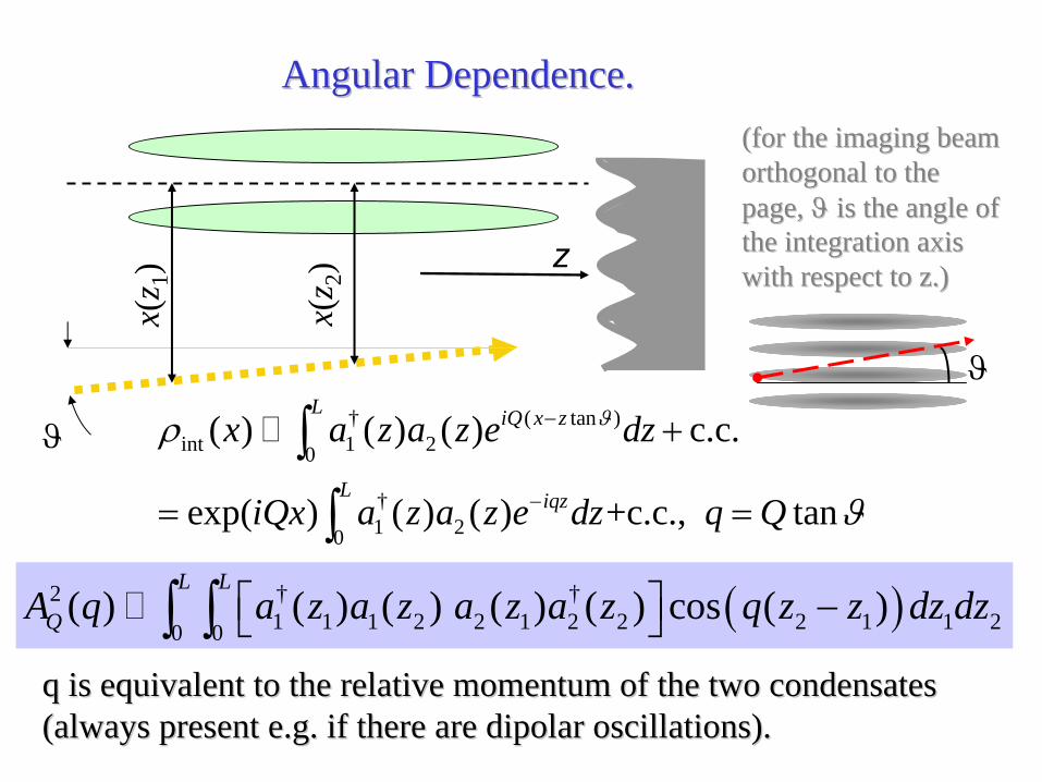
Angular Dependence.Angular Dependence.

† ( tan )int 1 20

†1 20

( ) ( ) ( ) c.c.

exp( ) ( ) ( ) +c.c., tan

L iQ x z

L iqz

x a z a z e dz

iQx a z a z e dz q Q

ϑρ

ϑ

−

−

+

= =

∫∫

( )2 † †1 1 1 2 2 1 2 2 2 1 1 20 0

( ) ( ) ( ) ( ) ( ) cos ( )L L

QA q a z a z a z a z q z z dz dz⎡ ⎤ −⎣ ⎦∫ ∫q is equivalent to the relative momentum of the two condensates q is equivalent to the relative momentum of the two condensates (always present e.g. if there are dipolar oscillations).(always present e.g. if there are dipolar oscillations).

ϑ

z

x(z 1

)

x(z 2

)

(for the imaging beam (for the imaging beam orthogonal to the orthogonal to the page, page, ϑϑ

is the angle of is the angle of

the integration axis the integration axis with respect to z.)with respect to z.)

ϑ

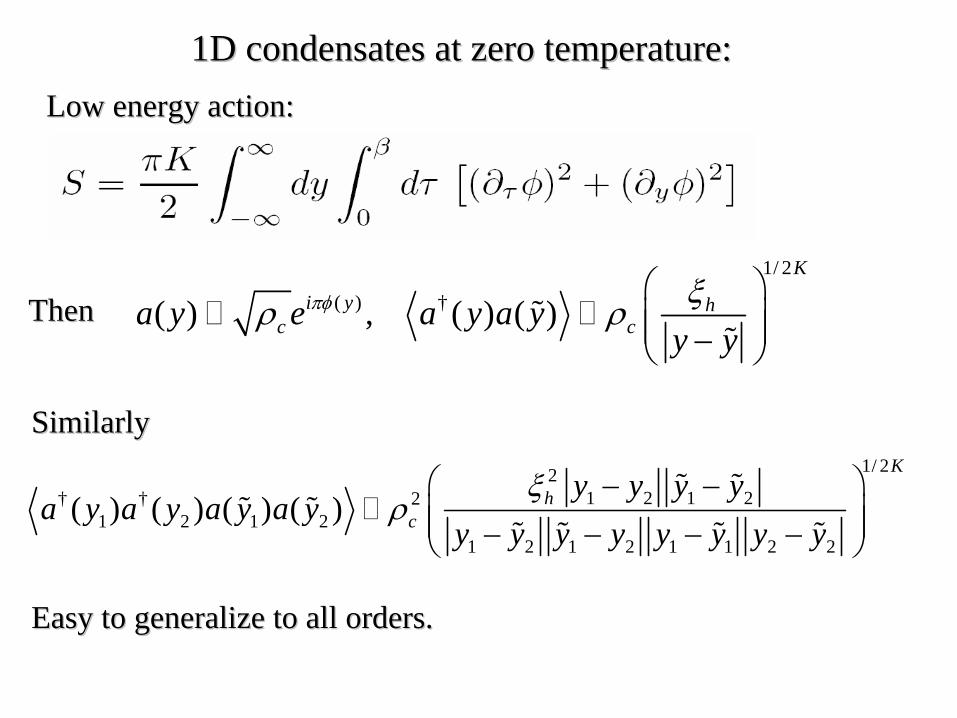
1D condensates at zero temperature:1D condensates at zero temperature:Low energy action:Low energy action:

ThenThen1/ 2

( ) †( ) , ( ) ( )K

i y hc ca y e a y a y

y yπφ ξρ ρ

⎛ ⎞⎜ ⎟⎜ ⎟−⎝ ⎠

%%

SimilarlySimilarly1/ 22

1 2 1 2† † 21 2 1 2

1 2 1 2 1 1 2 2

( ) ( ) ( ) ( )K

hc

y y y ya y a y a y a y

y y y y y y y yξ

ρ⎛ ⎞− −⎜ ⎟⎜ ⎟− − − −⎝ ⎠

% %% %

% % % %

Easy to generalize to all orders.Easy to generalize to all orders.

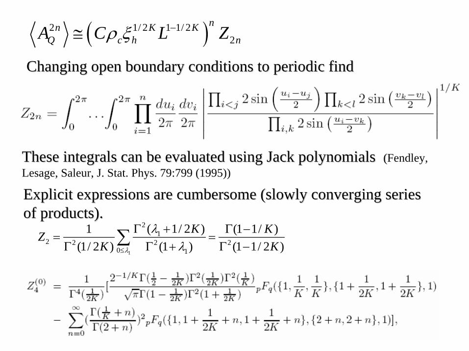
Changing open boundary conditions to periodic findChanging open boundary conditions to periodic find

( )2 1/ 2 1 1/ 22

nn K KQ c h nA C L Zρ ξ −≅

These integrals can be evaluated using Jack polynomials These integrals can be evaluated using Jack polynomials ((Fendley, Lesage, Saleur, J. Stat. Phys. 79:799 (1995))

Explicit expressions are cumbersome (slowly converging series Explicit expressions are cumbersome (slowly converging series of products).of products).

1

21

2 2 2 20 1

( 1/ 2 )1 (1 1/ )(1/ 2 ) (1 ) (1 1/ 2 )

K KZK Kλ

λλ≤

Γ + Γ −= =

Γ Γ + Γ −∑

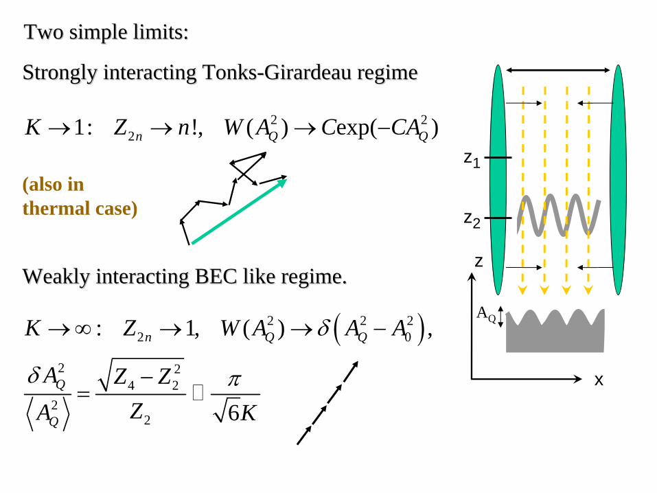
Two simple limits:Two simple limits:

2 221: !, ( ) exp( )n Q QK Z n W A C CA→ → → −

(also in thermal case)

x

z

z1

z2

AQ( )2 2 22 0

2 24 2

22

: 1, ( ) ,

6

n Q Q

Q

Q

K Z W A A A

A Z ZZA K

δ

δ π

→ ∞ → → −

−=

Strongly interacting Strongly interacting TonksTonks--Girardeau regimeGirardeau regime

Weakly interacting BEC like regime.Weakly interacting BEC like regime.

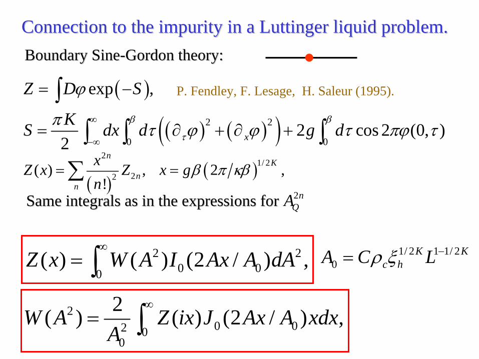
Connection to the impurity in a Connection to the impurity in a LuttingerLuttinger liquid problem.liquid problem.Boundary SineBoundary Sine--Gordon theory:Gordon theory:

( )

( ) ( )( )2 2

0 0

exp ,

2 cos 2 (0, )2 x

Z D S

KS dx d g dβ β

τ

ϕ

π τ ϕ ϕ τ πϕ τ∞

−∞

= −

= ∂ + ∂ +

∫

∫ ∫ ∫

( )( )

21/ 2

22( ) , 2 ,!

nK

nn

xZ x Z x gn

β π κβ= =∑Same integrals as in the expressions forSame integrals as in the expressions for 2n

QA

2 20 00

( ) ( ) (2 / ) ,Z x W A I Ax A dA∞

= ∫1/ 2 1 1/ 2

0K K

c hA C Lρ ξ −=

P. Fendley, F. Lesage, H. Saleur (1995).

20 02 0

0

2( ) ( ) (2 / ) ,W A Z ix J Ax A xdxA

∞= ∫

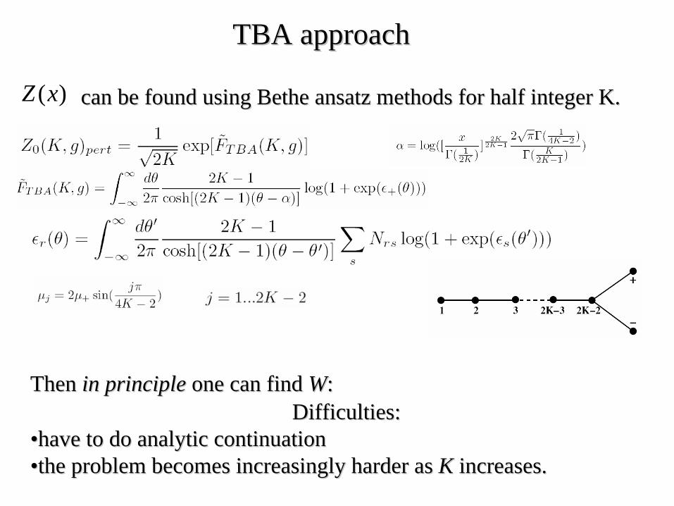
( )Z x can be found using can be found using BetheBethe ansatzansatz methods for half integer K.methods for half integer K.

Then Then in principlein principle one can find one can find WW::Difficulties:Difficulties:

••have to do analytic continuation have to do analytic continuation ••the problem becomes increasingly harder as the problem becomes increasingly harder as K K increases.increases.

TBA approachTBA approach

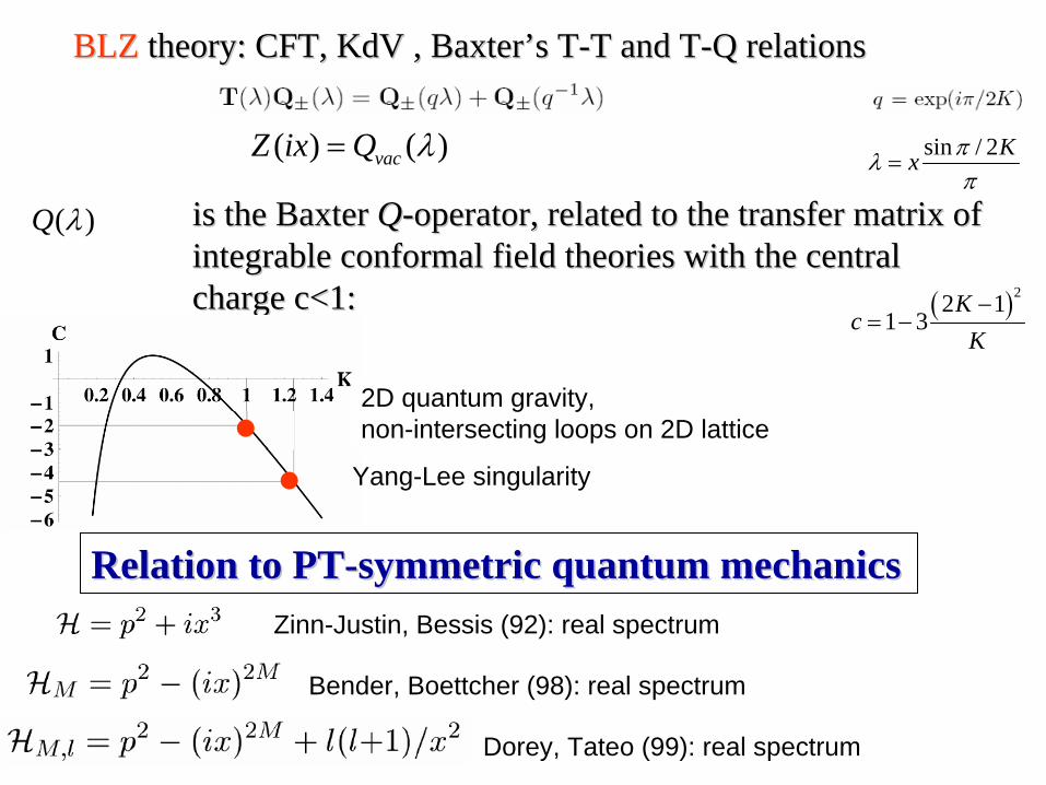
Relation to PTRelation to PT--symmetric quantum mechanicssymmetric quantum mechanics

( ) ( )vacZ ix Q λ= sin / 2Kx πλπ

=

( )Q λ is the Baxter is the Baxter QQ--operator, related to the transfer matrix of operator, related to the transfer matrix of integrableintegrable conformal field theories with the central conformal field theories with the central charge c<1:charge c<1:

Yang-Lee singularity

2D quantum gravity,non-intersecting loops on 2D lattice

( )22 11 3

Kc

K−

= −

BLZBLZ theory: CFT, theory: CFT, KdVKdV , Baxter’s T, Baxter’s T--T and TT and T--Q relationsQ relations

Zinn-Justin, Bessis (92): real spectrum

Bender, Boettcher (98): real spectrum

Dorey, Tateo (99): real spectrum

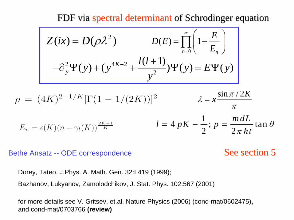
FDF via FDF via spectral determinantspectral determinant of of SchrodingerSchrodinger equationequation

Dorey, Tateo, J.Phys. A. Math. Gen. 32:L419 (1999);

Bazhanov, Lukyanov, Zamolodchikov, J. Stat. Phys. 102:567 (2001)

0

( ) 1n n

ED EE

∞

=

⎛ ⎞= −⎜ ⎟

⎝ ⎠∏

sin / 2Kx πλπ

=

for more details see V. Gritsev, et.al. Nature Physics (2006) (cond-mat/0602475), and cond-mat/0703766 (review)

2 4 22

( 1)( ) ( ) ( ) ( )Ky

l ly y y E yy

− +−∂ Ψ + + Ψ = Ψ

14 ; tan2 2

m dLl pK pt

θπ

= − =h

See section 5See section 5Bethe Ansatz -- ODE correspondence

2( ) ( )Z ix D ρλ=

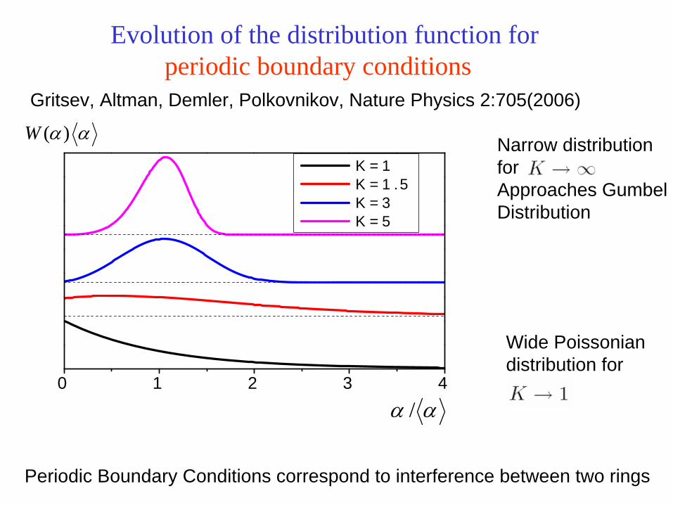
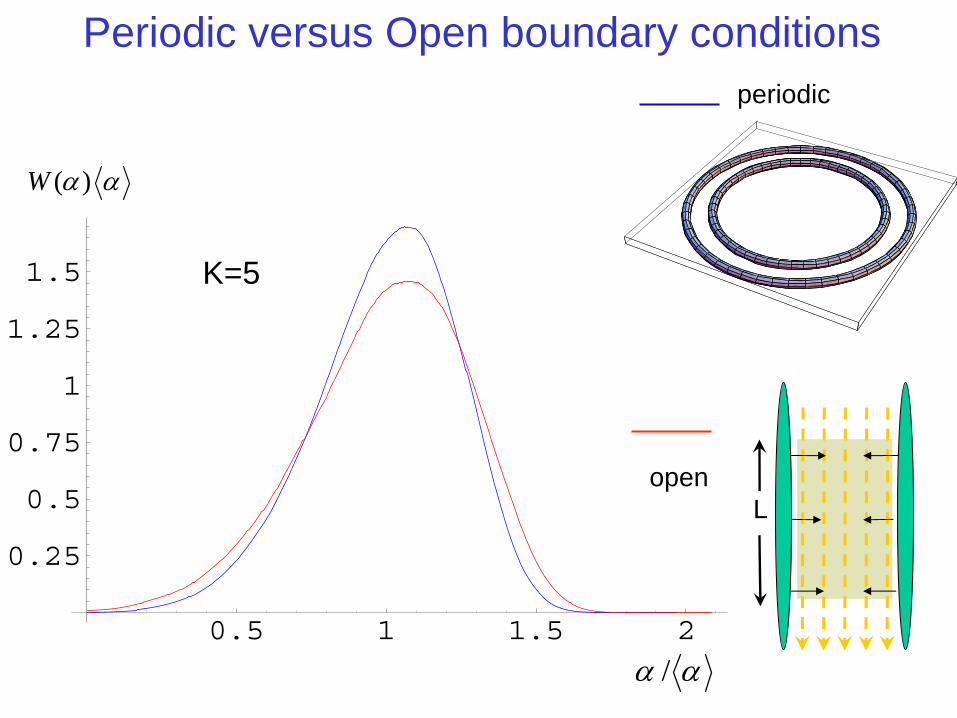
Evolution of the distribution function for periodic boundary conditions

Narrow distributionfor .Approaches GumbelDistribution

Wide Poissoniandistribution for

Gritsev, Altman, Demler, Polkovnikov, Nature Physics 2:705(2006)

αα /

Periodic Boundary Conditions correspond to interference between two rings

0 1 2 3 4

Pro

babi

lity

P(x

)

x

K = 1 K = 1 .5 K = 3 K = 5

αα )(W

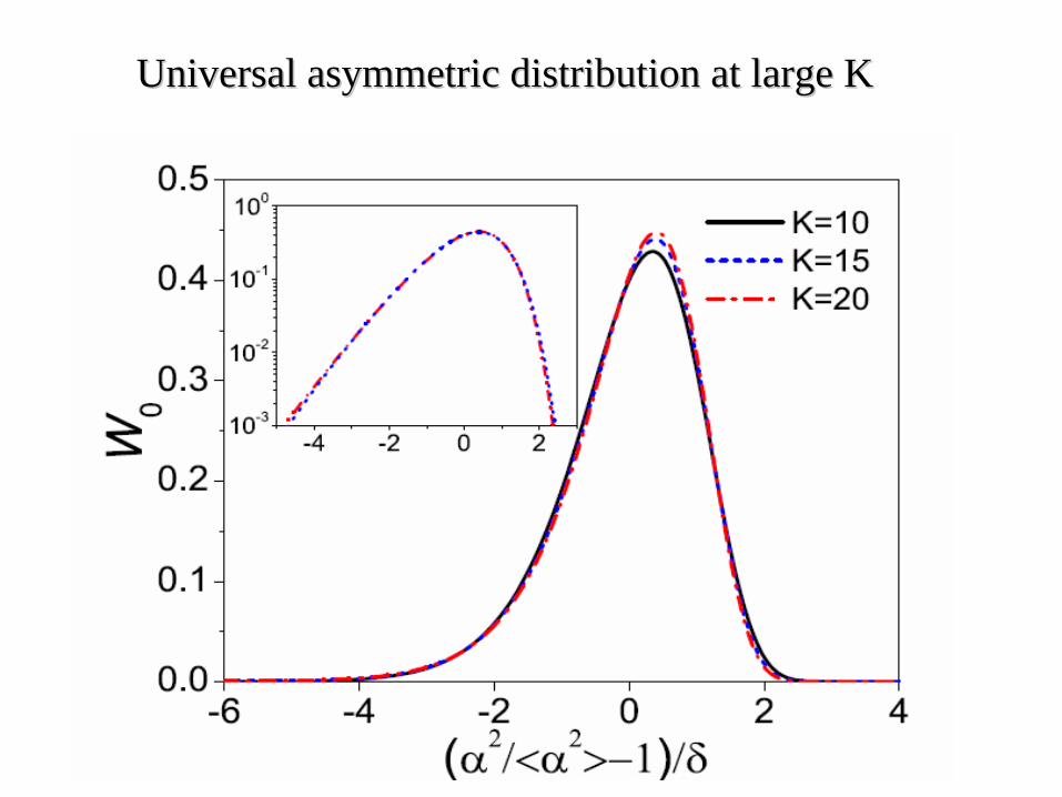
Universal asymmetric distribution at large KUniversal asymmetric distribution at large K

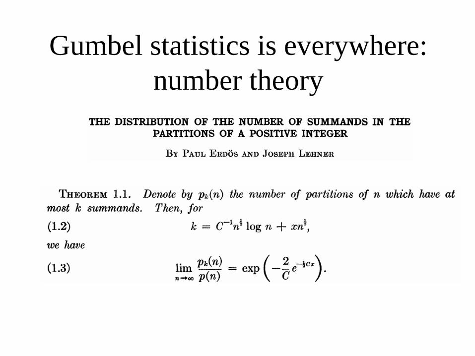
Gumbel statistics is everywhere: number theory

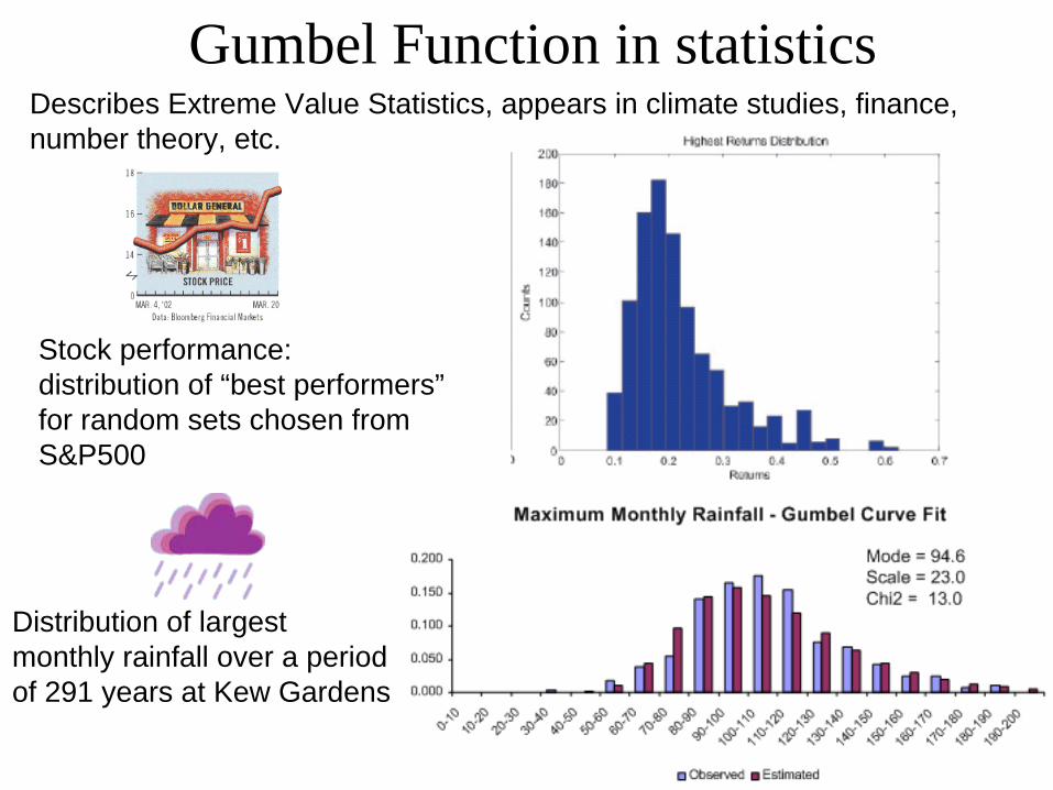
Gumbel Function in statisticsDescribes Extreme Value Statistics, appears in climate studies, finance, number theory, etc.

Stock performance: distribution of “best performers”for random sets chosen from S&P500

Distribution of largest monthly rainfall over a periodof 291 years at Kew Gardens

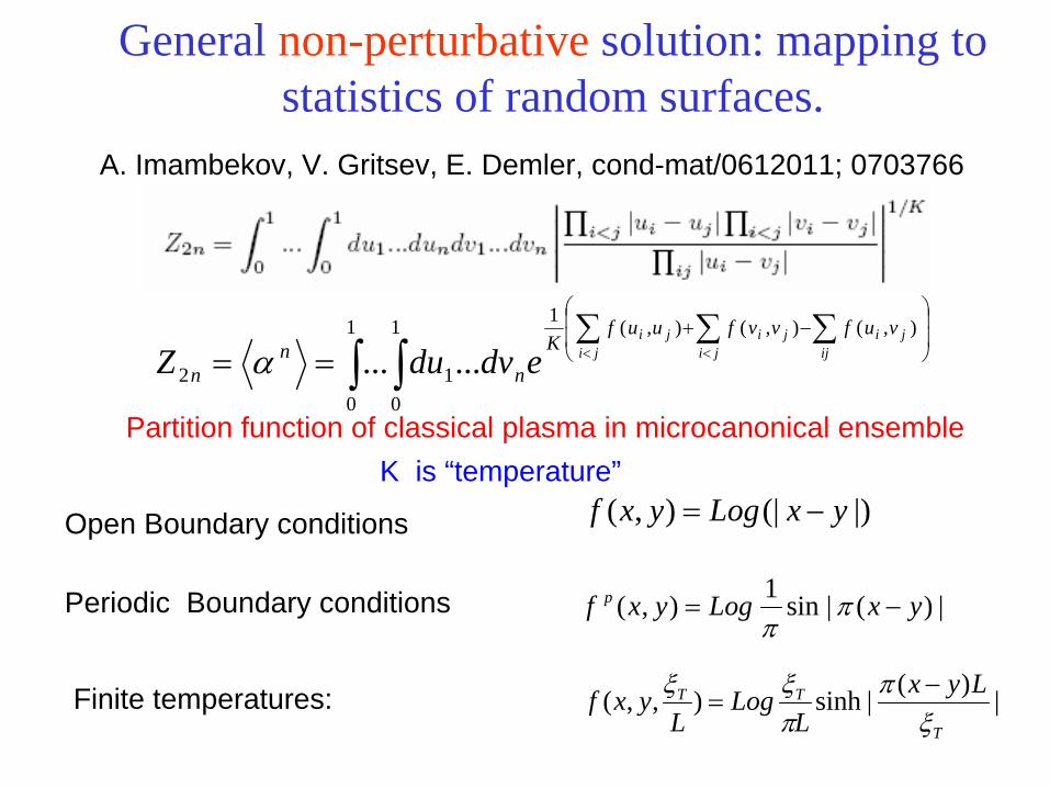
General non-perturbative solution: mapping to statistics of random surfaces.

|)(|sin1),( yxLogyxf p −= ππ

A. Imambekov, V. Gritsev, E. Demler, cond-mat/0612011; 0703766

Partition function of classical plasma in microcanonical ensemble

|)(|sinh),,(T

TT LyxL

LogL

yxfξ

ππξξ −

=

Open Boundary conditions

Periodic Boundary conditions

Finite temperatures:

⎟⎟

⎠

⎞

⎜⎜

⎝

⎛−+∑ ∑∑

== <<∫∫ ji ijjiji

jiji vufvvfuuf

Kn

nn edvduZ

),(),(),(11

01

1

02 ......α

|)(|),( yxLogyxf −=K is “temperature”

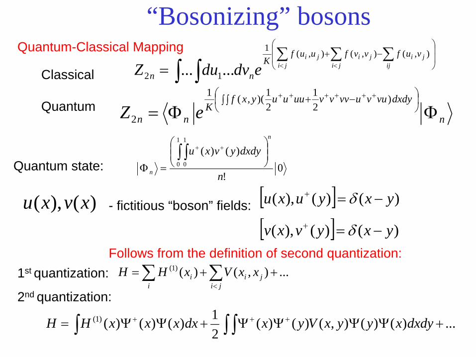
“Bosonizing” bosons⎟⎟

⎠

⎞

⎜⎜

⎝

⎛−+∑ ∑∑

= <<∫∫ ji ijjiji

jiji vufvvfuuf

Knn edvduZ

),(),(),(1

12 ......

n

dxdyvuvuvvvvuuuuyxfK

nn eZ ΦΦ=⎟⎠⎞

⎜⎝⎛

∫ ∫ −+ ++++++ )21

21)(,(1

2

Classical

Quantum

Quantum-Classical Mapping

0!

)()(1

0

1

0

n

dxdyyvxun

n

⎟⎟⎠

⎞⎜⎜⎝

⎛

=Φ∫ ∫ ++

Quantum state:

)(),( xvxu - fictitious “boson” fields: [ ] )()(),( yxyuxu −=+ δ

[ ] )()(),( yxyvxv −=+ δFollows from the definition of second quantization:

∑∑<

++=ji

jii

i xxVxHH ...),()()1(

...)()(),()()(21)()()()1( +ΨΨΨΨ+ΨΨ= ∫ ∫∫ +++ dxdyxyyxVyxdxxxxHH

1st quantization:

2nd quantization:

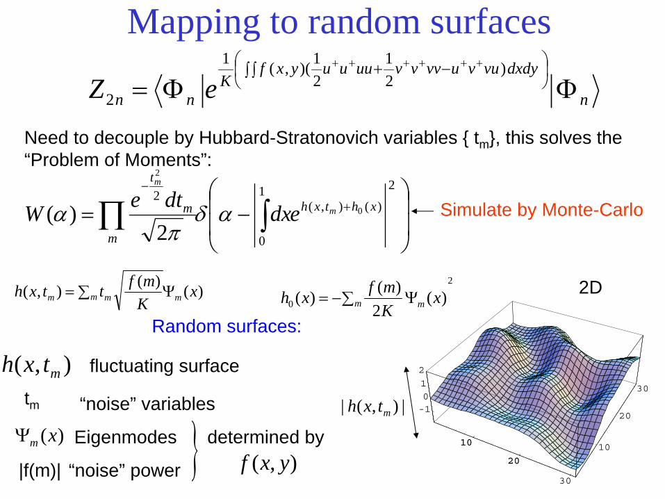
Mapping to random surfaces

),( yxf

Need to decouple by Hubbard-Stratonovich variables { tm }, this solves the “Problem of Moments”:

∑ Ψ= m mmm xKmfttxh )()(),(

)(xmΨ

|f(m)|

tm “noise” variables

Eigenmodes

“noise” power } determined by

Simulate by Monte-Carlo

10

20

30

10

20

30

-101

2

10

20

|),(| mtxh

Random surfaces:

2D

⎟⎟

⎠

⎞

⎜⎜

⎝

⎛−= +

−

∫∏2

)(),(1

0

20

2

2)( xhtxh

m

m

t

m

m

edxdteW αδπ

α

2

0 )(2

)()( ∑ Ψ−= m m xKmfxh

),( mtxh fluctuating surface

n

dxdyvuvuvvvvuuuuyxfK

nn eZ ΦΦ=⎟⎠⎞

⎜⎝⎛

∫ ∫ −+ ++++++ )21

21)(,(1

2

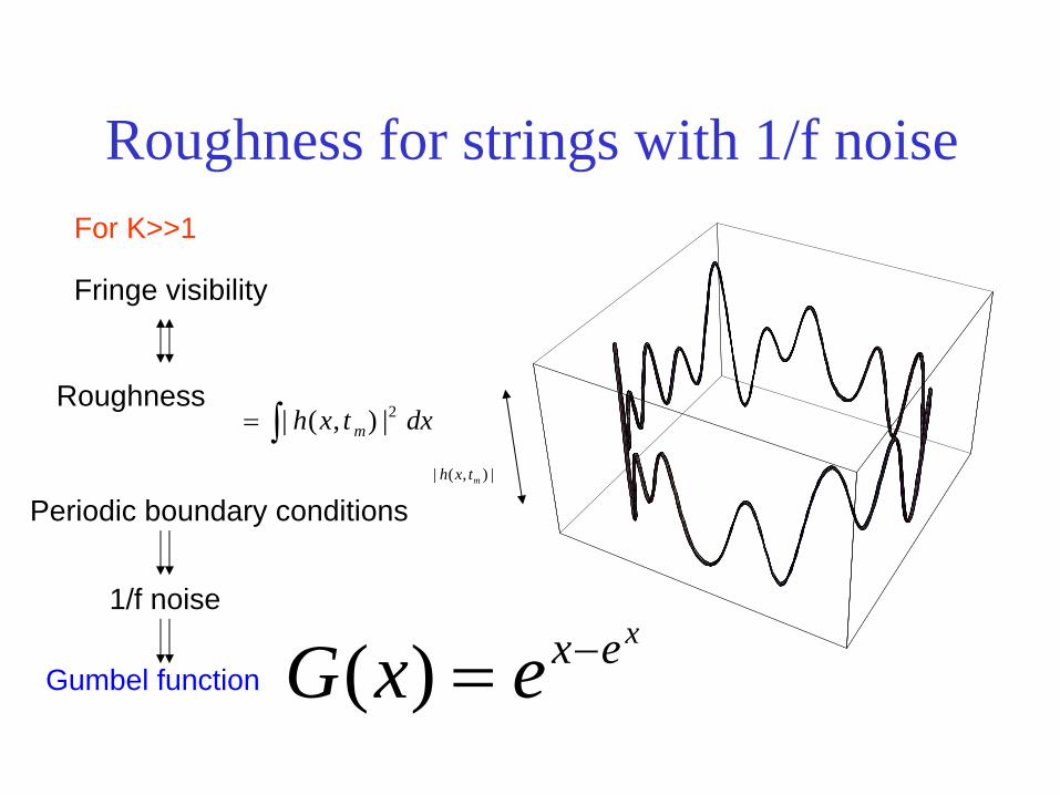
Roughness for strings with 1/f noise

dxtxh m2|),(|∫=

xexexG −=)(

Fringe visibility

Roughness

For K>>1

Periodic boundary conditions

1/f noise

Gumbel function

|),(| mtxh

0.5 1 1.5 2

0.25

0.5

0.75

1

1.25

1.5

Periodic versus Open boundary conditions

K=5

periodic

openL

αα /

αα )(W

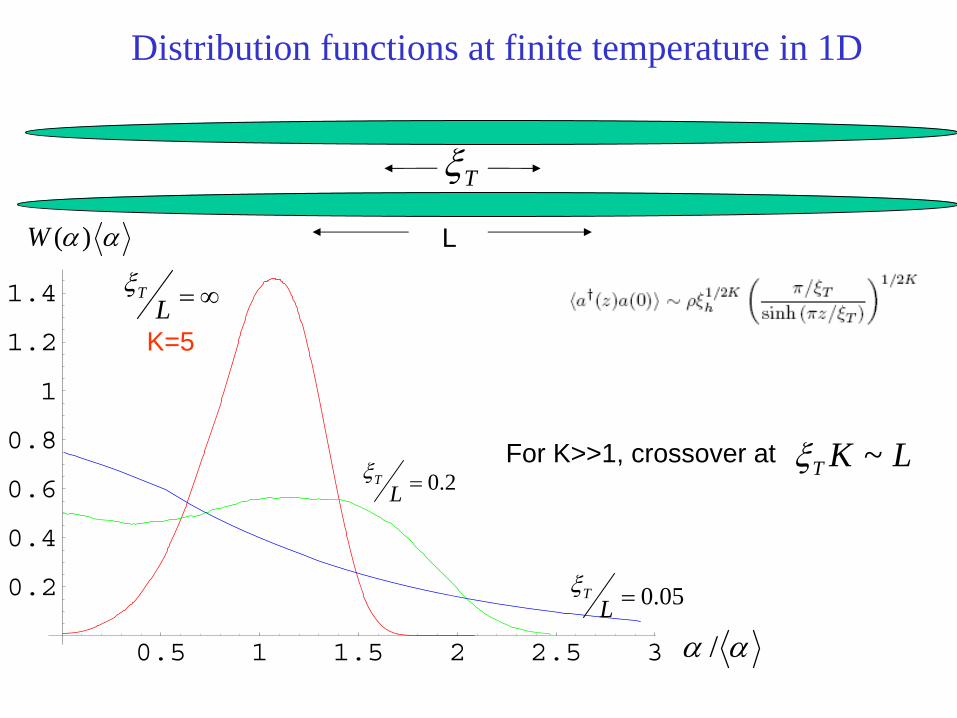
Distribution functions at finite temperature in 1D

Tξ

L

∞=LTξ

2.0=LTξ

0.5 1 1.5 2 2.5 3

0.2

0.4

0.6

0.8

1

1.2

1.4

05.0=LTξ

For K>>1, crossover at LKT ~ξ

K=5

αα /

αα )(W

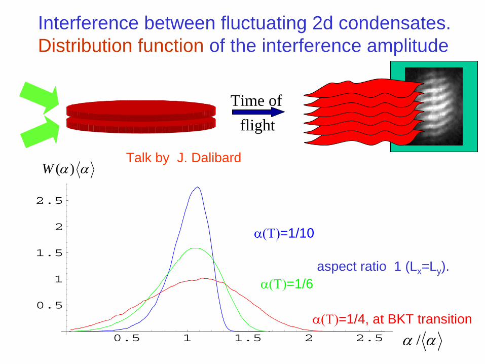
Interference between fluctuating 2d condensates.Distribution function of the interference amplitude

0.5 1 1.5 2 2.5

0.5

1

1.5

2

2.5

α(Τ)=1/10

α(Τ)=1/6

α(Τ)=1/4, at BKT transition

Time offlight

aspect ratio 1 (Lx =Ly ).

Talk by J. Dalibard

αα /

αα )(W

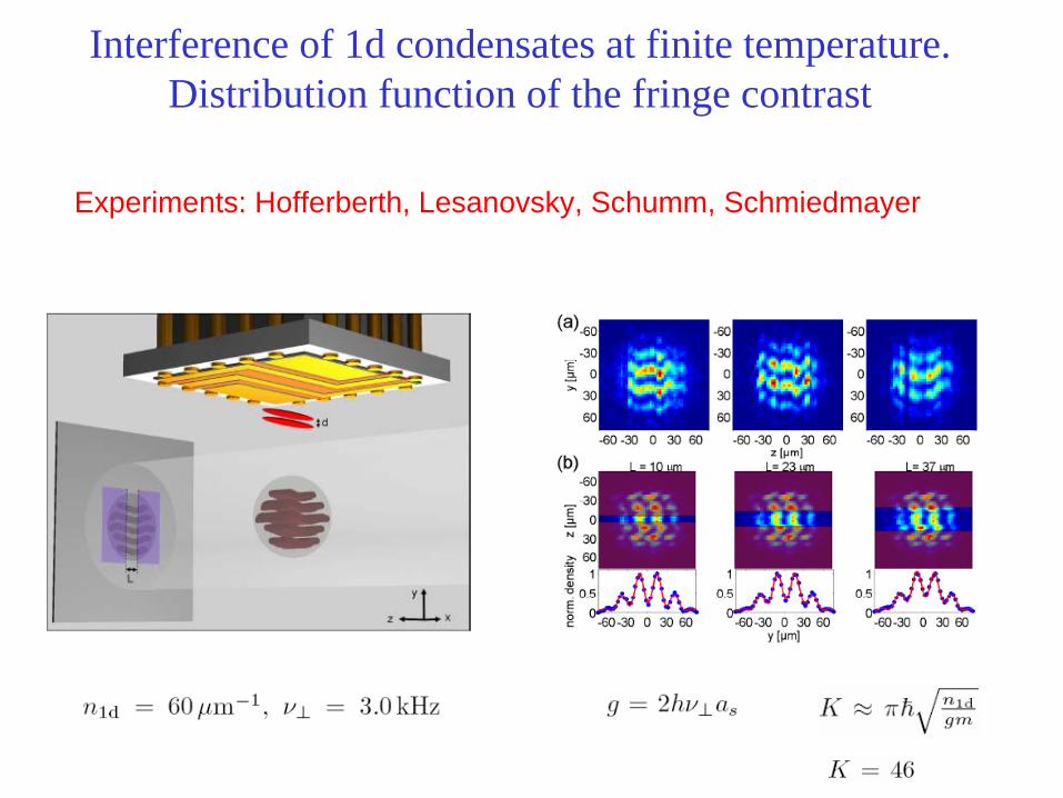
Experiments: Hofferberth, Lesanovsky, Schumm, Schmiedmayer

Interference of 1d condensates at finite temperature. Distribution function of the fringe contrast

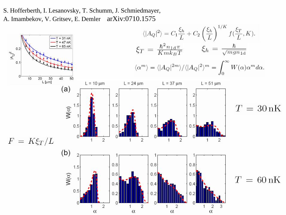
S. Hofferberth, I. Lesanovsky, T. Schumm, J. Schmiedmayer, A. Imambekov, V. Gritsev, E. Demler arXiv:0710.1575

4. FDF and other problems

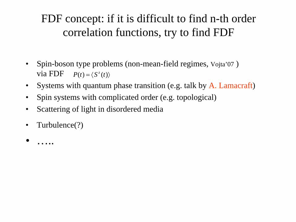
FDF concept: if it is difficult to find n-th order correlation functions, try to find FDF

• Spin-boson type problems (non-mean-field regimes, Vojta’07 ) via FDF

• Systems with quantum phase transition (e.g. talk by A. Lamacraft)• Spin systems with complicated order (e.g. topological)• Scattering of light in disordered media

• Turbulence(?)

• …..

( ) ( )zP t S t= ⟨ ⟩

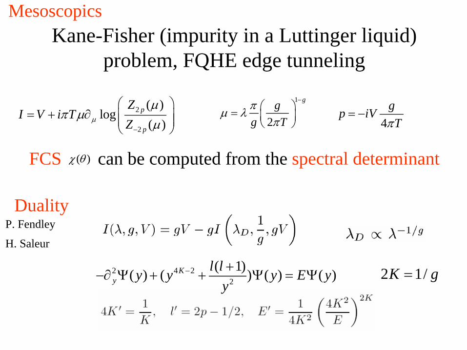
Kane-Fisher (impurity in a Luttinger liquid) problem, FQHE edge tunneling

2 4 22

( 1)( ) ( ) ( ) ( )Ky

l ly y y E yy

− +−∂ Ψ + + Ψ = Ψ

DualityP. Fendley

H. Saleur

2

2

( )log

( )p

p

ZI V i T

Zμ

μπ μ

μ−

⎛ ⎞= + ∂ ⎜ ⎟⎜ ⎟

⎝ ⎠

1

2

ggg Tπμ λ

π

−⎛ ⎞= ⎜ ⎟⎝ ⎠ 4

gp iVTπ

= −

2 1/K g=

FCS can be computed from the spectral determinant( )χ θ

Mesoscopics

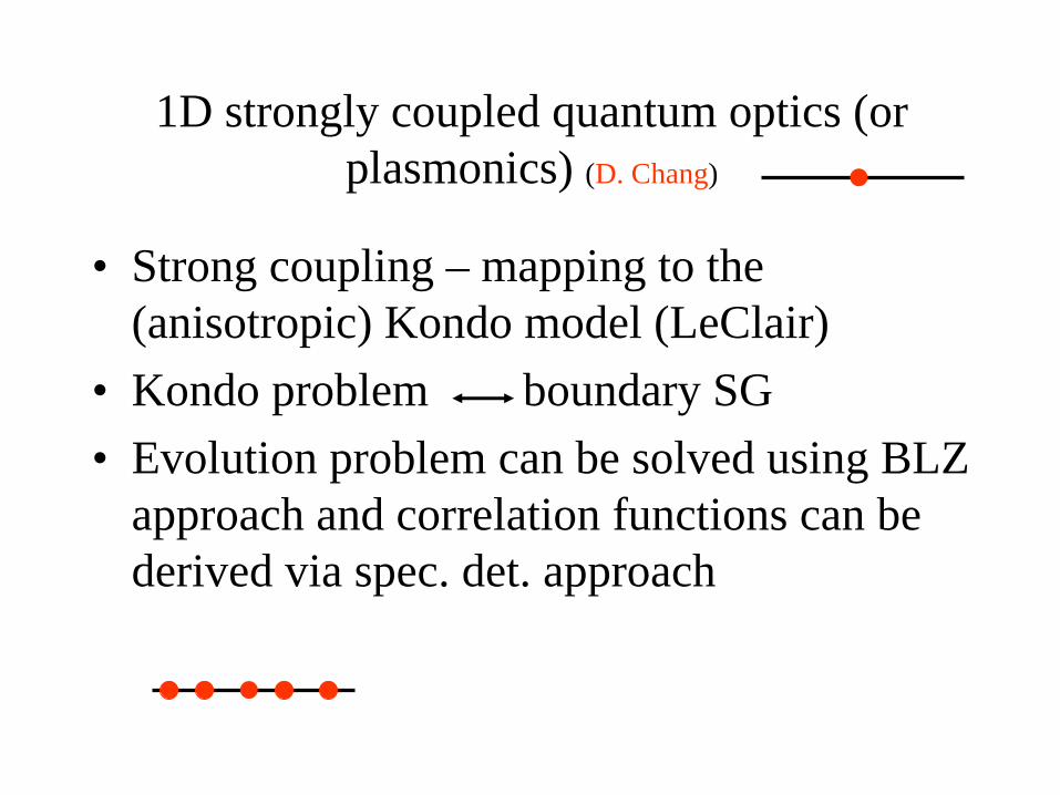
1D strongly coupled quantum optics (or plasmonics) (D. Chang)

• Strong coupling – mapping to the (anisotropic) Kondo model (LeClair)

• Kondo problem boundary SG• Evolution problem can be solved using BLZ

approach and correlation functions can be derived via spec. det. approach

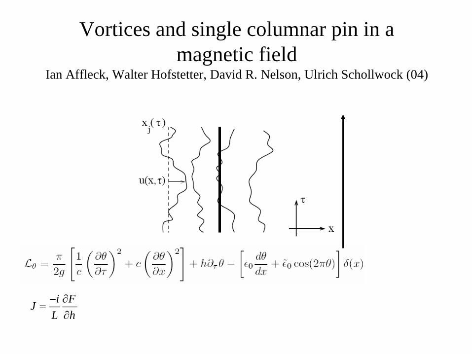
Vortices and single columnar pin in a magnetic field

Ian Affleck, Walter Hofstetter, David R. Nelson, Ulrich Schollwock (04)

i FJL h− ∂

=∂

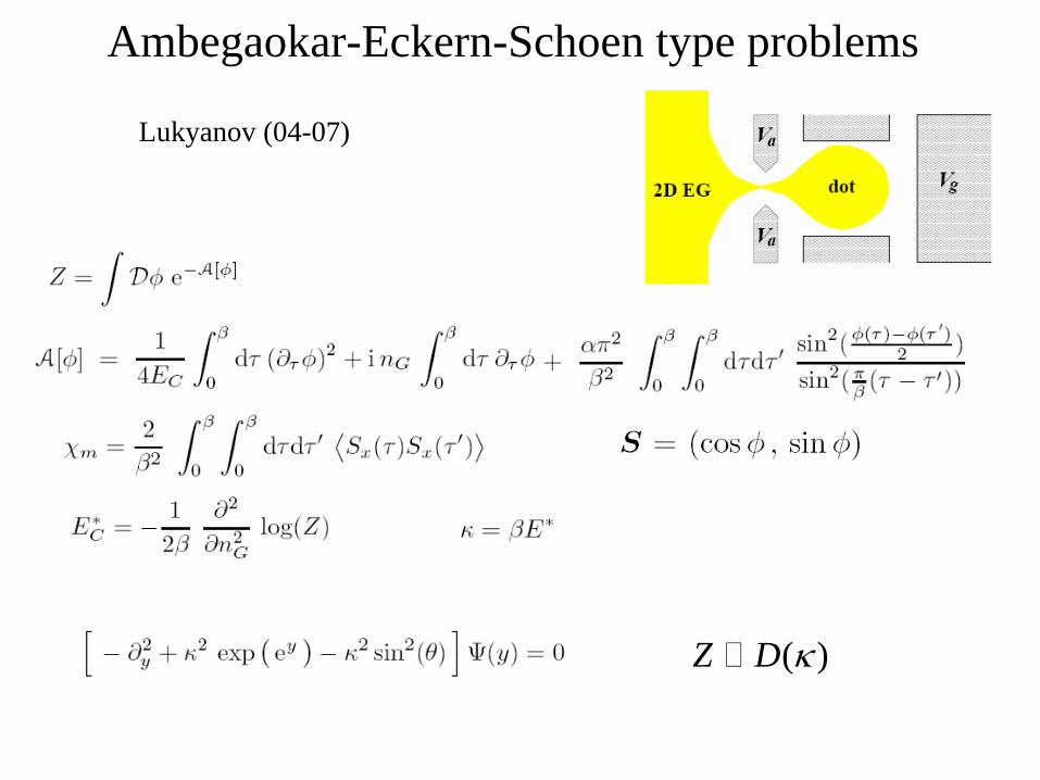
Ambegaokar-Eckern-Schoen type problems

( )Z D κ

Lukyanov (04-07)

5. FDF and AdS/CFT correspondence

FDF and Langlands duality

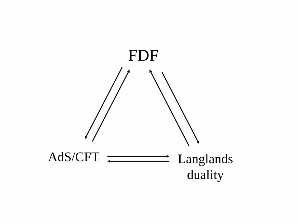
FDF

AdS/CFT Langlands duality

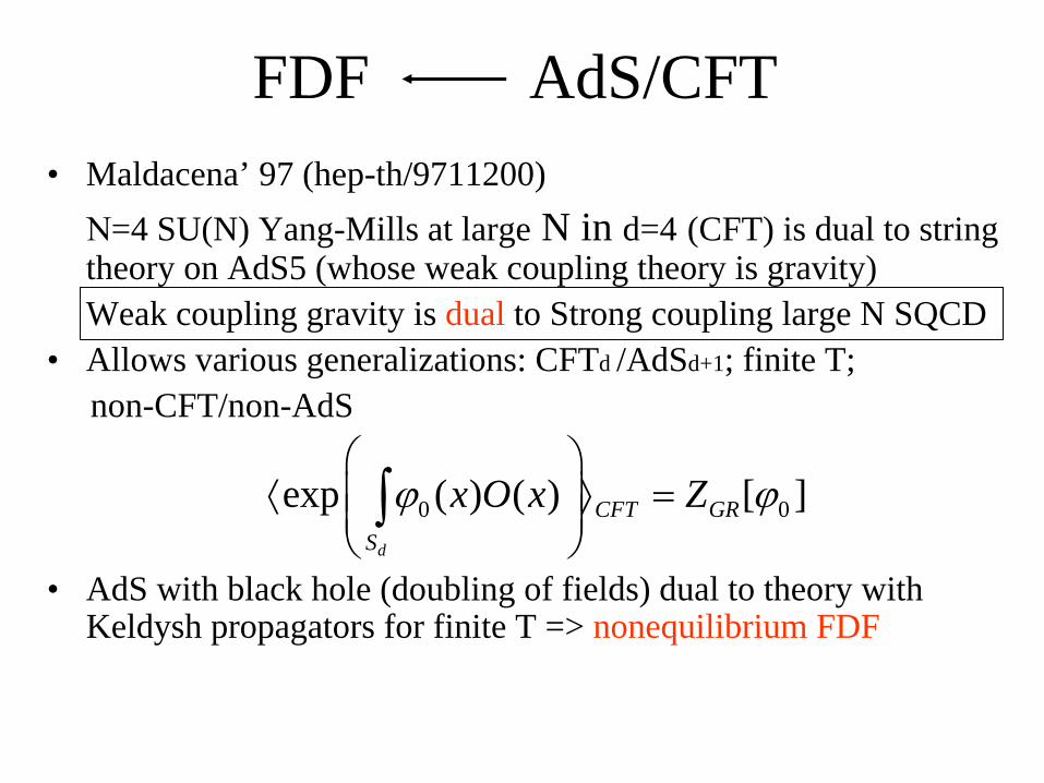
FDF AdS/CFT• Maldacena’ 97 (hep-th/9711200) Ν=4 SU(N) Yang-Mills at large N in d=4 (CFT) is dual to string

theory on AdS5 (whose weak coupling theory is gravity) Weak coupling gravity is dual to Strong coupling large N SQCD• Allows various generalizations: CFTd /AdSd+1; finite T;

non-CFT/non-AdS

• AdS with black hole (doubling of fields) dual to theory with Keldysh propagators for finite T => nonequilibrium FDF

0 0exp ( ) ( ) [ ]d

CFT GRS

x O x Zϕ ϕ⎛ ⎞

⟨ ⟩ =⎜ ⎟⎜ ⎟⎝ ⎠∫

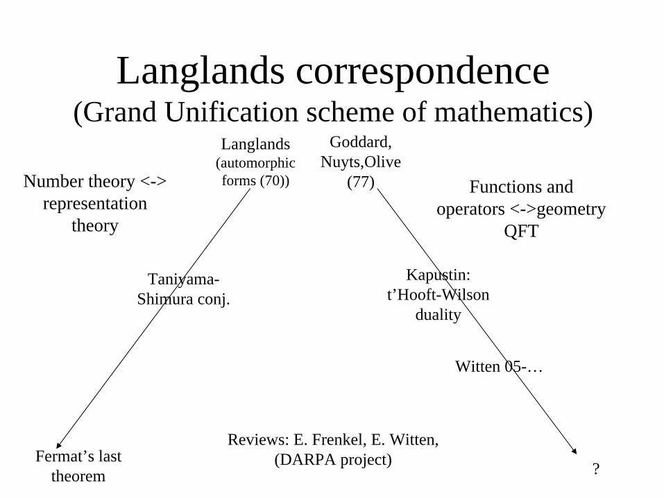
Langlands correspondence (Grand Unification scheme of mathematics)

Number theory <-> representation

theory

Functions and operators <->geometry

QFT

Langlands(automorphic forms (70))

Taniyama- Shimura conj.

Fermat’s last theorem

Goddard, Nuyts,Olive

(77)

Kapustin: t’Hooft-Wilson

duality

Witten 05-…

?

Reviews: E. Frenkel, E. Witten, (DARPA project)

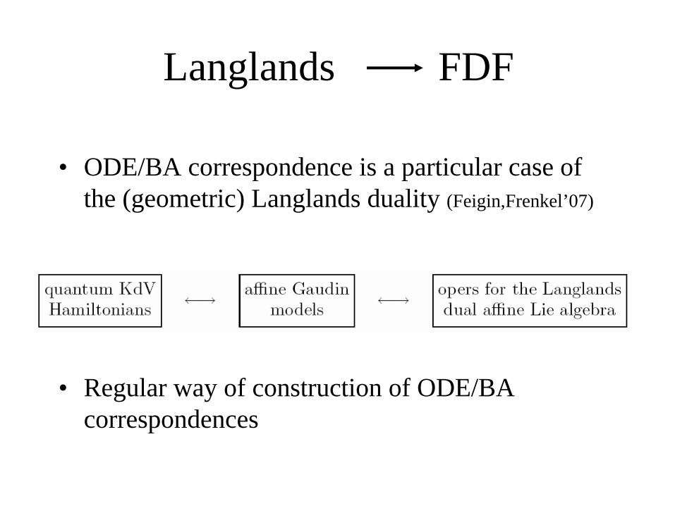
• ODE/BA correspondence is a particular case of the (geometric) Langlands duality (Feigin,Frenkel’07)

• Regular way of construction of ODE/BA correspondences

Langlands FDF

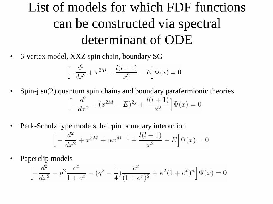
• 6-vertex model, XXZ spin chain, boundary SG

• Spin-j su(2) quantum spin chains and boundary parafermionic theories

• Perk-Schulz type models, hairpin boundary interaction

• Paperclip models

List of models for which FDF functions can be constructed via spectral

determinant of ODE

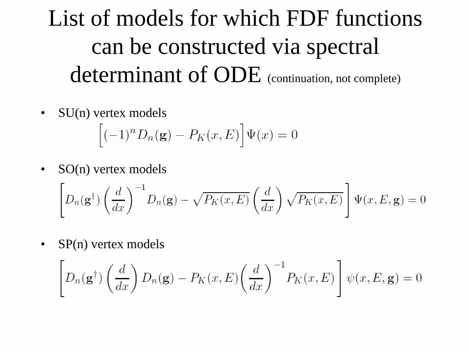
List of models for which FDF functions can be constructed via spectral

determinant of ODE (continuation, not complete)

• SU(n) vertex models

• SO(n) vertex models

• SP(n) vertex models

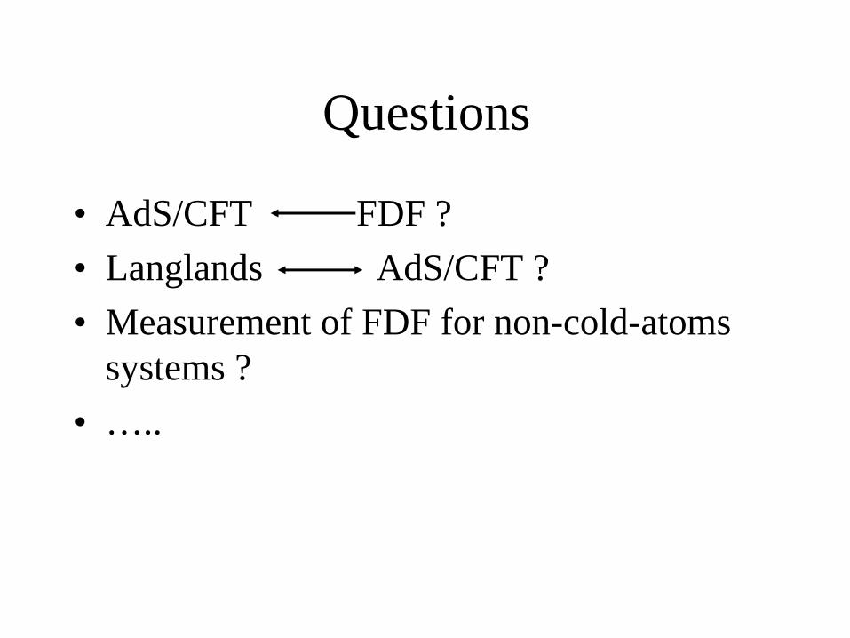
Questions

• AdS/CFT FDF ?• Langlands AdS/CFT ?• Measurement of FDF for non-cold-atoms

systems ?• …..